P1: OSO FREE013-25 FREE013-Moore September 9, 2008 13:51 CONFIRMING C H A P T E R 25 Nonparametric Tests Ariel Skelly/CORBIS IN THIS CHAPTER WE COVER... ■ Comparing two samples: the Wilcoxon rank sum test ■ The Normal approximation for W ■ Using technology ■ What hypotheses does Wilcoxon test? ■ Dealing with ties in rank tests ■ Matched pairs: the Wilcoxon signed rank test ■ The Normal approximation for W + ■ Dealing with ties in the signed rank test ■ Comparing several samples: the Kruskal-Wallis test ■ Hypotheses and conditions for the Kruskal-Wallis test ■ The Kruskal-Wallis test statistic The most commonly used methods for inference about the means of quantitative response variables assume that the variables in question have Normal distribu- tions in the population or populations from which we draw our data. In practice, of course, no distribution is exactly Normal. Fortunately, our usual methods for inference about population means (the one-sample and two-sample t procedures and analysis of variance) are quite robust. That is, the results of inference are robustness not very sensitive to moderate lack of Normality, especially when the samples are reasonably large. Practical guidelines for taking advantage of the robustness of these methods appear in Chapters 17, 18, and 24. What can we do if plots suggest that the data are clearly not Normal, especially when we have only a few observations? This is not a simple question. Here are the basic options: 1. If lack of Normality is due to outliers, it may be legitimate to remove out- liers if you have reason to think that they do not come from the same pop- ulation as the other observations. Equipment failure that produced a bad measurement, for example, entitles you to remove the outlier and analyze the remaining data. But if an outlier appears to be “real data,” you should not CAUTION arbitrarily remove it. 2. In some settings, other standard distributions replace the Normal distribu- tions as models for the overall pattern in the population. The lifetimes in 25-1
Transcript
P1: OSO
FREE013-25 FREE013-Moore September 9, 2008 13:51
CONFIRMING
C H A P T E R 25
Nonparametric Tests
Ari
elSk
elly
/CO
RB
IS
I N T H I S C H A P T E R
W E C O V E R . . .
■ Comparing two samples: theWilcoxon rank sum test
■ The Normal approximation for W
■ Using technology
■ What hypotheses does Wilcoxontest?
■ Dealing with ties in rank tests
■ Matched pairs: the Wilcoxonsigned rank test
■ The Normal approximation for W +
■ Dealing with ties in the signedrank test
■ Comparing several samples: theKruskal-Wallis test
■ Hypotheses and conditions for theKruskal-Wallis test
■ The Kruskal-Wallis test statistic
The most commonly used methods for inference about the means of quantitativeresponse variables assume that the variables in question have Normal distribu-tions in the population or populations from which we draw our data. In practice,of course, no distribution is exactly Normal. Fortunately, our usual methods forinference about population means (the one-sample and two-sample t proceduresand analysis of variance) are quite robust. That is, the results of inference arerobustness
not very sensitive to moderate lack of Normality, especially when the samplesare reasonably large. Practical guidelines for taking advantage of the robustnessof these methods appear in Chapters 17, 18, and 24.
What can we do if plots suggest that the data are clearly not Normal, especiallywhen we have only a few observations? This is not a simple question. Here arethe basic options:
1. If lack of Normality is due to outliers, it may be legitimate to remove out-liers if you have reason to think that they do not come from the same pop-ulation as the other observations. Equipment failure that produced a badmeasurement, for example, entitles you to remove the outlier and analyzethe remaining data. But if an outlier appears to be “real data,”you should notCAUTION
arbitrarily remove it.
2. In some settings, other standard distributions replace the Normal distribu-tions as models for the overall pattern in the population. The lifetimes in
25-1
P1: OSO
FREE013-25 FREE013-Moore August 25, 2008 16:4
REVISED PAGE
25-2 CHAPTER 25 • Nonparametric Tests
service of equipment or the survival times of cancer patients after treatmentusually have right-skewed distributions. Statistical studies in these areas usefamilies of right-skewed distributions rather than Normal distributions. Thereare inference procedures for the parameters of these distributions that replacethe t procedures.
3. Modern bootstrap methods and permutation tests use heavy computing toavoid requiring Normality or any other specific form of sampling distribution.We recommend these methods unless the sample is so small that it may notrepresent the population well. For an introduction, see Companion Chapter16 of the somewhat more advanced text Introduction to the Practice of Statistics,available online at www.whfreeman.com/ips.
4. Finally, there are other nonparametric methods, which do not assume anyspecific form for the distribution of the population. Unlike bootstrap and per-mutation methods, common nonparametric methods do not make use of theactual values of the observations.
This chapter concerns one type of nonparametric procedure: tests that can re-place the t tests and one-way analysis of variance when the Normality conditionsfor those tests are not met. The most useful nonparametric tests are rank testsrank tests
based on the rank (place in order) of each observation in the set of all the data.Figure 25.1 presents an outline of the standard tests (based on Normal distribu-
tions) and the rank tests that compete with them. The rank tests require that thepopulation or populations have continuous distributions. That is, each distributionmust be described by a density curve (Chapter 3, page 69) that allows observationsto take any value in some interval of outcomes. The Normal curves are one shapeof density curve. Rank tests allow curves of any shape.
The rank tests we will study concern the center of a population or populations.When a population has at least roughly a Normal distribution, we describe itscenter by the mean. The “Normal tests” in Figure 25.1 all test hypotheses aboutpopulation means. When distributions are strongly skewed, we often prefer themedian to the mean as a measure of center. In simplest form, the hypotheses forrank tests just replace mean by median.
Setting Normal test Rank test
One sample Wilcoxon signed rank test
Wilcoxon rank sum test
Kruskal-Wallis testOne-way ANOVA F testChapter 24
One-sample t testChapter 17
Matched pairs Apply one-sample test to differences within pairs
Two independent samples Two-sample t testChapter 18
Several independent samples
FIGURE 25.1
Comparison of tests based on Normal distributions with rank tests for similar settings.
P1: OSO
FREE013-25 FREE013-Moore August 25, 2008 16:4
REVISED PAGE
• Comparing two samples: the Wilcoxon rank sum test 25-3
We begin by describing the most common rank test, for comparing two sam-ples. In this setting we also explain ideas common to all rank tests: the big ideaof using ranks, the conditions required by rank tests, the nature of the hypothesestested, and the contrast between exact distributions for use with small samples andNormal approximations for use with larger samples.
Comparing two samples: the Wilcoxon
rank sum test
Two-sample problems (see Chapter 18) are among the most common in statistics.The most useful nonparametric significance test compares two distributions. Here
ST
EP
is an example of this setting.
Weeds among the cornE X A M P L E 25.1
STATE: Does the presence of small numbers of weeds reduce the yield of corn? Lamb’s-quarter is a common weed in corn fields. A researcher planted corn at the same ratein 8 small plots of ground, then weeded the corn rows by hand to allow no weeds in4 randomly selected plots and exactly 3 lamb’s-quarter plants per meter of row in theother 4 plots. Here are the yields of corn (bushels per acre) in each of the plots:1
0 weeds per meter 166.7 172.2 165.0 176.9
3 weeds per meter 158.6 176.4 153.1 156.0
PLAN: Make a graph to compare the two sets of yields. Test the hypothesis that thereis no difference against the one-sided alternative that yields are higher when no weedsare present.
SOLVE (first steps): A back-to-back stemplot (Figure 25.2) suggests that yields maybe higher when there are no weeds. There is one outlier; because it is correct data, wecannot remove it. The samples are too small to rely on the robustness of the two-samplet test. We will now develop a test that does not require Normality. ■
3 weeds/meter0 weeds/meter
7 5 2 7
15 15 16 16 1717
3 6 9
6
FIGURE 25.2
Back-to-back stemplot of corn yieldsfrom plots with no weeds and with3 weeds per meter of row, for Exam-ple 25.1. Notice the split stems, withleaves 0 to 4 on the first stem andleaves 5 to 9 on the second stem.
First, arrange all 8 observations from both samples in order from smallest tolargest:
153.1 156.0 158.6 165.0 166.7 172.2 176.4 176.9
P1: OSO
FREE013-25 FREE013-Moore August 25, 2008 16:4
REVISED PAGE
25-4 CHAPTER 25 • Nonparametric Tests
The boldface entries in the list are the yields with no weeds present. We seethat four of the five highest yields come from that group, suggesting that yieldsare higher with no weeds. The idea of rank tests is to look just at position in thisordered list. To do this, replace each observation by its order, from 1 (smallest) to8 (largest). These numbers are the ranks:
To rank observations, first arrange them in order from smallest to largest. The rankof each observation is its position in this ordered list, starting with rank 1 for thesmallest observation.
Moving from the original observations to their ranks retains only the ordering ofthe observations and makes no other use of their numerical values. Working withranks allows us to dispense with specific conditions on the shape of the distribution,such as Normality.
If the presence of weeds reduces corn yields, we expect the ranks of the yieldsfrom plots without weeds to be larger as a group than the ranks from plots withweeds. Let’s compare the sums of the ranks from the two treatments:
Treatment Sum of ranks
No weeds 23Weeds 13
These sums measure how much the ranks of the weed-free plots as a group ex-ceed those of the weedy plots. In fact, the sum of the ranks from 1 to 8 is alwaysequal to 36, so it is enough to report the sum for one of the two groups. If the sumof the ranks for the weed-free group is 23, the ranks for the other group must addto 13 because 23 + 13 = 36. If the weeds have no effect, we would expect the sumof the ranks in either group to be 18 (half of 36). Here are the facts we need in amore general form that takes account of the fact that our two samples need not bethe same size.
T H E W I L C O X O N R A N K S U M T E S T
Draw an SRS of size n1 from one population and draw an independent SRS of sizen2 from a second population. There are N observations in all, where N = n1 + n2.Rank all N observations. The sum W of the ranks for the first sample is the Wilcoxonrank sum statistic. If the two populations have the same continuous distribution,then W has mean
μW = n1(N + 1)2
P1: OSO
FREE013-25 FREE013-Moore September 9, 2008 13:51
CONFIRMING
• Comparing two samples: the Wilcoxon rank sum test 25-5
and standard deviation
σW =√
n1n2(N + 1)12
The Wilcoxon rank sum test rejects the hypothesis that the two populations haveidentical distributions when the rank sum W is far from its mean.
In the corn yield study of Example 25.1, we want to test the hypotheses
H0 : no difference in distribution of yieldsHa : yields are systematically higher in weed-free plots
Our test statistic is the rank sum W = 23 for the weed-free plots.
ST
EP
Weeds among the corn: inferenceE X A M P L E 25.2
SOLVE: First note that the conditions for the Wilcoxon test are met: the data come froma randomized comparative experiment and the yield of corn in bushels per acre has acontinuous distribution.
There are N = 8 observations in all, with n1 = 4 and n2 = 4. The sum of ranks forthe weed-free plots has mean
μW = n1(N + 1)2
= (4)(9)2
= 18
and standard deviation
σW =√
n1n2(N + 1)12
=√
(4)(4)(9)12
=√
12 = 3.464
Although the observed rank sum W = 23 is higher than the mean, it is only about 1.4standard deviations higher. We now suspect that the data do not give strong evidencethat yields are higher in the population of weed-free corn.
The P -value for our one-sided alternative is P (W ≥ 23), the probability that W isat least as large as the value for our data when H0 is true. Software tells us that thisprobability is P = 0.1.
CONCLUDE: The data provide some evidence (P = 0.1) that corn yields are lowerwhen weeds are present. There are only 4 observations in each group, so even quitelarge effects can fail to reach the levels of significance usually considered convinc-ing, such as P < 0.05. A larger experiment might clarify the effect of weeds on cornyield. ■
P1: OSO
FREE013-25 FREE013-Moore August 25, 2008 16:4
REVISED PAGE
25-6 CHAPTER 25 • Nonparametric Tests
A P P L Y Y O U R K N O W L E D G E
25.1 Daily activity and obesity. Our lead example for the two-sample t proceduresin Chapter 18 concerned a study comparing the level of physical activity of leanand mildly obese people who don’t exercise. Here are the minutes per day that thesubjects spent standing or walking over a 10-day period:
The data are a bit irregular but not distinctly non-Normal. Let’s use the Wilcoxontest for comparison with the two-sample t test.
(a) Find the median minutes spent standing or walking for each group. Whichgroup appears more active?
(b) Arrange all 20 observations in order and find the ranks.
(c) Take W to be the sum of the ranks for the lean group. What is the value ofW? If the null hypothesis (no difference between the groups) is true, whatare the mean and standard deviation of W?
(d) Does comparing W with the mean and standard deviation suggest that thelean subjects are more active than the obese subjects?
25.2 How strong are durable press fabrics? Exercise 18.38 (text page 496) describesan experiment comparing the strengths of cotton fabric treated with two “durablepress” processes. Here are the breaking strengths in pounds:
Permafresh 29.9 30.7 30.0 29.5 27.6
Hylite 28.8 23.9 27.0 22.1 24.2
There is a mild outlier in the Permafresh group. Perhaps we should use theWilcoxon test.
(a) Arrange the breaking strengths in order and find their ranks.
(b) Find the Wilcoxon statistic W for the Permafresh group, along with its meanand standard deviation under the null hypothesis (no difference between thegroups).
(c) Is W far enough from the mean to suggest that there may be a differencebetween the groups?
The Normal approximation for W
To calculate the P -value P (W ≥ 23) for Example 25.2, we need to know thesampling distribution of the rank sum W when the null hypothesis is true. This
P1: OSO
FREE013-25 FREE013-Moore August 25, 2008 16:4
REVISED PAGE
• The Normal approximation for W 25-7
distribution depends on the two sample sizes n1 and n2. Tables are therefore un-wieldy. Most statistical software will give you P -values, as well as carry out theranking and calculate W. However, many software packages give only approxi-mate P -values. You must learn what your software offers.
With or without software, P -values for the Wilcoxon test are often based onthe fact that the rank sum statistic W becomes approximately Normal as thetwo sample sizes increase. We can then form yet another z statistic by standardiz-ing W:
z = W − μW
σW
= W − n1(N + 1)/2√n1n2(N + 1)/12
Use standard Normal probability calculations to find P -values for this statistic.Because W takes only whole-number values, an idea called the continuity correctionimproves the accuracy of the approximation.
C O N T I N U I T Y C O R R E C T I O N
To apply the continuity correction in a Normal approximation for a variable thattakes only whole-number values, act as if each whole number occupies the entireinterval from 0.5 below the number to 0.5 above it.
Weeds among the corn: Normal approximationE X A M P L E 25.3
The standardized rank sum statistic W in our corn yield example is
z = W − μW
σW= 23 − 18
3.464= 1.44
We expect W to be larger when the alternative hypothesis is true, so the approximateP -value is (from Table A)
P (Z ≥ 1.44) = 0.0749
We can improve this approximation by using the continuity correction. To do this,act as if the whole number 23 occupies the entire interval from 22.5 to 23.5. Calculatethe P -value P (W ≥ 23) as P (W ≥ 22.5) because the value 23 is included in the rangewhose probability we want. Here is the calculation:
P (W ≥ 22.5) = P(
W − μW
σW≥ 22.5 − 18
3.464
)
= P (Z ≥ 1.30)
= 0.0968
This is close to the software value, P = 0.1. If you do not use the exact distribution of W(from software or tables), you should always use the continuity correction in calculatingP -values. ■
P1: OSO
FREE013-25 FREE013-Moore September 9, 2008 13:51
CONFIRMING
25-8 CHAPTER 25 • Nonparametric Tests
A P P L Y Y O U R K N O W L E D G E
25.3 Daily activity and obesity, continued. In Exercise 25.1, you found the Wilcoxonrank sum W and its mean and standard deviation. We want to test the null hypoth-esis that the two groups don’t differ in activity against the alternative hypothesisthat the lean subjects spend more time standing and walking.
(a) What is the probability expression for the P -value of W if we use the conti-nuity correction?
(b) Find the P -value. What do you conclude?
25.4 Strength of durable press fabrics, continued. Use your values of W, μW, andσW from Exercise 25.2 to see whether fabrics treated with the two processes differin breaking strength.
(a) The two-sided P -value is 2P (W ≥ ?). Using the continuity correction, whatnumber replaces the ? in this probability?
(b) Find the P -value. What do you conclude?
Ariel Skelly/CORBIS
25.5 Tell me a story. A study of early childhood education asked kindergarten studentsS
TE
P
to tell fairy tales that had been read to them earlier in the week. The 10 children inthe study included 5 high-progress readers and 5 low-progress readers. Each childtold two stories. Story 1 had been read to them; Story 2 had been read and alsoillustrated with pictures. An expert listened to a recording of the children andassigned a score for certain uses of language. Here are the data:2
Child Progress Story 1 score Story 2 score
1 high 0.55 0.802 high 0.57 0.823 high 0.72 0.544 high 0.70 0.795 high 0.84 0.896 low 0.40 0.777 low 0.72 0.498 low 0.00 0.669 low 0.36 0.28
10 low 0.55 0.38
Look only at the data for Story 2. Is there good evidence that high-progress readersscore higher than low-progress readers? Follow the four-step process as illustratedin Examples 25.1 and 25.2.
Using technology
For samples as small as those in the corn yield study of Example 25.1, we prefersoftware that gives the exact P -value for the Wilcoxon test rather than the Normalapproximation. Neither the Excel spreadsheet nor TI graphing calculators havemenu entries for rank tests. Minitab offers only the Normal approximation.
P1: OSO
FREE013-25 FREE013-Moore August 25, 2008 16:4
REVISED PAGE
• Using technology 25-9
Weeds among the corn: software outputE X A M P L E 25.4
Figure 25.3 displays output from CrunchIt! for the corn yield data. The top panel reportsthe exact Wilcoxon P -value as P = 0.1. The Normal approximation with continuitycorrection, P = 0.0968 in Example 25.3, is quite accurate. There are several differencesbetween the CrunchIt! output and our work in Example 25.3. The most important isthat CrunchIt! carries out the Mann-Whitney test rather than the Wilcoxon test. Mann-Whitney test
The two tests always have the same P -value because the two test statistics are relatedby simple algebra.
The second panel in Figure 25.3 is the two-sample t test from Chapter 18, which doesnot assume that the two populations have the same standard deviation. It gives P =0.0937, close to the Wilcoxon value. Because the t test is quite robust, it is somewhatunusual for P -values from t and W to differ greatly.
The bottom panel shows the result of the “pooled” version of t , now outdated, thatassumes equal population standard deviations. You see that its P is a bit different fromthe others, another reminder that you should never use this test. ■
A P P L Y Y O U R K N O W L E D G E
25.6 Strength of durable press fabrics: software. Use your software to repeat theWilcoxon test you did in Exercise 25.4. By comparing the results, state how yoursoftware finds P -values for W: exact distribution, Normal approximation with con-tinuity correction, or Normal approximation without continuity correction.
25.7 Daily activity and obesity: software. Use your software to carry out the one-sided Wilcoxon rank sum test that you did by hand in Exercise 25.3. Use the exactdistribution if your software will do it. Compare the software result with your resultin Exercise 25.3.
25.8 Weeds among the corn. The corn yield study of Example 25.1 also examinedyields in four plots having 9 lamb’s-quarter plants per meter of row. The yields(bushels per acre) in these plots were
162.8 142.4 162.7 162.4
There is a clear outlier, but rechecking the results found that this is the correctyield for this plot. The outlier makes us hesitant to use t procedures because x ands are not resistant.
(a) Is there evidence that 9 weeds per meter reduces corn yields when comparedwith weed-free corn? Use the Wilcoxon rank sum test with the data aboveand part of the data from Example 25.1 to answer this question.
(b) Compare the results from (a) with those from the two-sample t test for thesedata.
(c) Now remove the low outlier 142.4 from the data with 9 weeds per me-ter. Repeat both the Wilcoxon and t analyses. By how much did the out-lier reduce the mean yield in its group? By how much did it increase thestandard deviation? Did it have a practically important impact on yourconclusions?
P1: OSO
FREE013-25 FREE013-Moore August 25, 2008 16:4
REVISED PAGE
25-10 CHAPTER 25 • Nonparametric Tests
Mann-Whitney
Two sample T statistics
Two sample T statistics
FIGURE 25.3
Output from CrunchIt! for the data of Example 25.1. The output compares the results of three teststhat could be used to compare yields for the two groups of corn plots.
P1: OSO
FREE013-25 FREE013-Moore September 9, 2008 13:51
CONFIRMING
• What hypotheses does Wilcoxon test? 25-11
What hypotheses does Wilcoxon test?
Our null hypothesis is that weeds do not affect yield. The alternative hypothesisis that yields are lower when weeds are present. If we are willing to assume thatyields are Normally distributed, or if we have reasonably large samples, we can usethe two-sample t test for means. Our hypotheses then have the form
H0 : μ1 = μ2
Ha : μ1 > μ2
When the distributions may not be Normal, we might restate the hypotheses interms of population medians rather than means:
H0 : median1 = median2
Ha : median1 > median2
The Wilcoxon rank sum test provides a test of these hypotheses, but only ifan additional condition is met: both populations must have distributions of thesame shape. That is, the density curve for corn yields with 3 weeds per meter looksexactly like that for no weeds except that it may slide to a different location onthe scale of yields. The CrunchIt! output in the top panel of Figure 25.3 states thehypotheses in terms of population medians. CrunchIt! will also give a confidenceinterval for the difference between the two population medians.
The same-shape condition is too strict to be reasonable in practice. Fortunately,the Wilcoxon test also applies in a more useful setting. It compares any two contin-uous distributions, whether or not they have the same shape, by testing hypothesesthat we can state in words as
H0: the two distributions are the sameHa : one has values that are systematically larger
A more exact statement of the “systematically larger” alternative hypothesis isa bit tricky, so we won’t try to give it here.3 These hypotheses really are “nonpara-metric” because they do not involve any specific parameter such as the mean ormedian. If the two distributions do have the same shape, the general hypothesesreduce to comparing medians. Many texts and computer outputs state the hypothe- CAUTION
ses in terms of medians, sometimes ignoring the same-shape condition. We recommendthat you express the hypotheses in words rather than symbols. “Yields are system-atically higher in weed-free plots” is easy to understand and is a good statement ofthe effect that the Wilcoxon test looks for.
Why don’t we discuss the confidence intervals for the difference in populationmedians that software such as CrunchIt! offers? These intervals require the unre-alistic same-shape condition. The more general “systematically larger” hypothesisdoes not involve a specific parameter, so there is no accompanying confidenceinterval.
P1: OSO
FREE013-25 FREE013-Moore August 25, 2008 16:4
REVISED PAGE
25-12 CHAPTER 25 • Nonparametric Tests
A P P L Y Y O U R K N O W L E D G E
25.9 Daily activity and obesity: hypotheses. We could use either two-sample t or theWilcoxon rank sum to test the null hypothesis that lean and mildly obese peopledon’t differ in the time they spend standing and walking against the alternativehypothesis that lean people generally spend more time in these activities. Explaincarefully what H0 and Ha are for t and for W.
25.10 Strength of durable press fabrics: hypotheses. We are interested in whetherfabrics treated with the Permafresh and Hylite processes have the same breakingstrength “on the average.”
(a) State null and alternative hypotheses in terms of population means. Whattest would we typically use for these hypotheses? What conditions does thistest require?
(b) State null and alternative hypotheses in terms of population medians. Whattest would we typically use for these hypotheses? What conditions does thistest require?
Dealing with ties in rank tests
We have chosen our examples and exercises to this point rather carefully: they allinvolve data in which no two values are the same. This allowed us to rank all thevalues. In practice, however, we often find observations tied at the same value.What shall we do? The usual practice is to assign all tied values the average of theaverage ranks
ranks they occupy. Here is an example with 6 observations:
The tied observations occupy the third and fourth places in the ordered list, sothey share rank 3.5.
The exact distribution for the Wilcoxon rank sum W applies only to data with-out ties. Moreover, the standard deviation σW must be adjusted if ties are present.The Normal approximation can be used after the standard deviation is adjusted.Statistical software will detect ties, make the necessary adjustment, and switch tothe Normal approximation. In practice, software is required to use rank tests when the
CAUTION data contain tied values.Some data have many ties because the scale of measurement has only a few
values. Rank tests are often used for such data. Here is an example.
ST
EP
Food safety at fairsE X A M P L E 25.5
STATE: Food sold at outdoor fairs and festivals may be less safe than food sold in restau-rants because it is prepared in temporary locations and often by volunteer help. What dopeople who attend fairs think about the safety of the food served? One study asked thisquestion of people at a number of fairs in the Midwest: “How often do you think people
P1: OSO
FREE013-25 FREE013-Moore August 25, 2008 16:4
REVISED PAGE
• Dealing with ties in rank tests 25-13
become sick because of food they consume prepared at outdoor fairs and festivals?”Thepossible responses were
1 = very rarely2 = once in a while3 = often4 = more often than not5 = always
In all, 303 people answered the question. Of these, 196 were women and 107 weremen.4 We suspect that women are more concerned than men about food safety. Is theregood evidence for this conclusion?
Danny Lehman/CORBIS
PLAN: Do data analysis to understand the difference between women and men. Checkthe conditions required by the Wilcoxon test. If the conditions are met, use theWilcoxon test for the hypotheses
H0: men and women do not differ in their responsesHa : women give systematically higher responses than men
SOLVE: The responses for the 303 subjects appear in the file eg25-05.dat on thetext CD and Web site. We can summarize them in a two-way table of counts:
Response
1 2 3 4 5 Total
Female 13 108 50 23 2 196Male 22 57 22 5 1 107
Total 35 165 72 28 3 303
Comparing row percents shows that the women in the sample do tend to give higherresponses (showing more concern):
Response
1 2 3 4 5 Total
Percent of females 6.6 55.1 25.5 11.7 1.0 100Percent of males 20.6 53.3 20.6 4.7 1.0 100
Are these differences between women and men statistically significant?The most important condition for inference is that the subjects are a random sample
of people who attend fairs, at least in the Midwest. The researcher visited 11 differentfairs. She stood near the entrance and stopped every 25th adult who passed. Becauseno personal choice was involved in choosing the subjects, we can reasonably treat thedata as coming from a random sample. (As usual, there was some nonresponse, whichcould create bias.) The Wilcoxon test also requires that responses have continuous dis-tributions. We think that the subjects really have a continuous distribution of opinionsabout how often people become sick from food at fairs. The questionnaire asks them toround off their opinions to the nearest value in the five-point scale. So we are willingto use the Wilcoxon test.
P1: OSO
FREE013-25 FREE013-Moore August 25, 2008 16:4
REVISED PAGE
25-14 CHAPTER 25 • Nonparametric Tests
Mann-Whitney
Two sample T statistics
FIGURE 25.4
Output from CrunchIt! for the dataof Example 25.5. The Wilcoxon ranksum test and the two-sample t testgive similar results.
Because the responses can take only five values, there are many ties. All 35 peoplewho chose “very rarely”are tied at 1, and all 165 who chose “once in a while”are tied at2. Figure 25.4 gives output from CrunchIt! The Wilcoxon (reported as Mann-Whitney)test for the one-sided alternative that women are more concerned about food safety atfairs is highly significant (P = 0.0004).
With more than 100 observations in each group and no outliers, we might use thetwo-sample t test even though responses take only five values. Figure 25.4 shows thatt = 3.3655 with P = 0.0005. The one-sided P -value for the two-sample t test is essen-tially the same as that for the Wilcoxon test.
CONCLUDE: There is very strong evidence (P = 0.0004) that women are more con-cerned than men about the safety of food served at fairs. ■
As is often the case, t and W for the data in Example 25.5 agree closely. Thereis, however, another reason to prefer the rank test in this example. The t statistictreats the response values 1 through 5 as meaningful numbers. In particular, the
P1: OSO
FREE013-25 FREE013-Moore August 25, 2008 16:4
REVISED PAGE
• Dealing with ties in rank tests 25-15
possible responses are treated as though they are equally spaced. The differencebetween “very rarely” and “once in a while” is the same as the difference between“once in a while” and “often.” This may not make sense. The rank test, on theother hand, uses only the order of the responses, not their actual values. The re-sponses are arranged in order from least to most concerned about safety, so therank test makes sense. Some statisticians avoid using t procedures when there is not a CAUTION
fully meaningful scale of measurement.Because we have a two-way table, we might have applied the chi-square test
(Chapter 22), which asks if there is a significant relationship of any kind betweengender and response. The chi-square test ignores the ordering of the responses andso doesn’t tell us whether women are more concerned than men about the safetyof the food served. This question depends on the ordering of responses from leastconcerned to most concerned.
A P P L Y Y O U R K N O W L E D G E
Software is required to adequately carry out the Wilcoxon rank sum test in the presence of ties.All of the following exercises concern data with ties.
25.11 Does polyester decay? Exercise 18.8 (text page 482) compares the breakingstrength of polyester strips buried for 16 weeks with that of strips buried for 2 weeks.The breaking strengths in pounds are
2 weeks 118 126 126 120 129
16 weeks 124 98 110 140 110
(a) What are the null and alternative hypotheses for the Wilcoxon test? For thetwo-sample t test?
(b) There are two pairs of tied observations. What ranks do you assign to eachobservation, using average ranks for ties?
(c) Apply the Wilcoxon rank sum test to these data. Compare your result withthe P = 0.1857 obtained from the two-sample t test in Figure 18.5.
25.12 Do birds learn to time their breeding? Exercises 18.42 to 18.44 (text pages 497–498) concern a study of whether supplementing the diet of blue titmice with extracaterpillars will prevent them from adjusting their breeding date the following yearin search of a better food supply. Here are the data (days after the caterpillar peak):
Control 4.6 2.3 7.7 6.0 4.6 −1.2
Supplemented 15.5 11.3 5.4 16.5 11.3 11.4 7.7
The null hypothesis is no difference in timing; the alternative hypothesis is thatthe supplemented birds miss the peak by more days because they don’t adjust theirbreeding date.
(a) There are three sets of ties, at 4.6, 7.7, and 11.3. Arrange the observations inorder and assign average ranks to each tied observation.
P1: OSO
FREE013-25 FREE013-Moore August 25, 2008 16:4
REVISED PAGE
25-16 CHAPTER 25 • Nonparametric Tests
(b) Take W to be the rank sum for the supplemented group. What is the valueof W?
(c) Use software: find the P -value of the Wilcoxon test and state your conclu-sion.
25.13 Tell me a story, continued. The data in Exercise 25.5 for a story told withoutpictures (Story 1) have tied observations. Is there good evidence that high-progressreaders score higher than low-progress readers when they retell a story they haveheard without pictures?
(a) Make a back-to-back stemplot of the 5 responses in each group. Are anymajor deviations from Normality apparent?
(b) Carry out a two-sample t test. State hypotheses and give the two samplemeans, the t statistic and its P -value, and your conclusion.
(c) Carry out the Wilcoxon rank sum test. State hypotheses and give the ranksum W for high-progress readers, its P -value, and your conclusion. Do the tand Wilcoxon tests lead you to different conclusions?
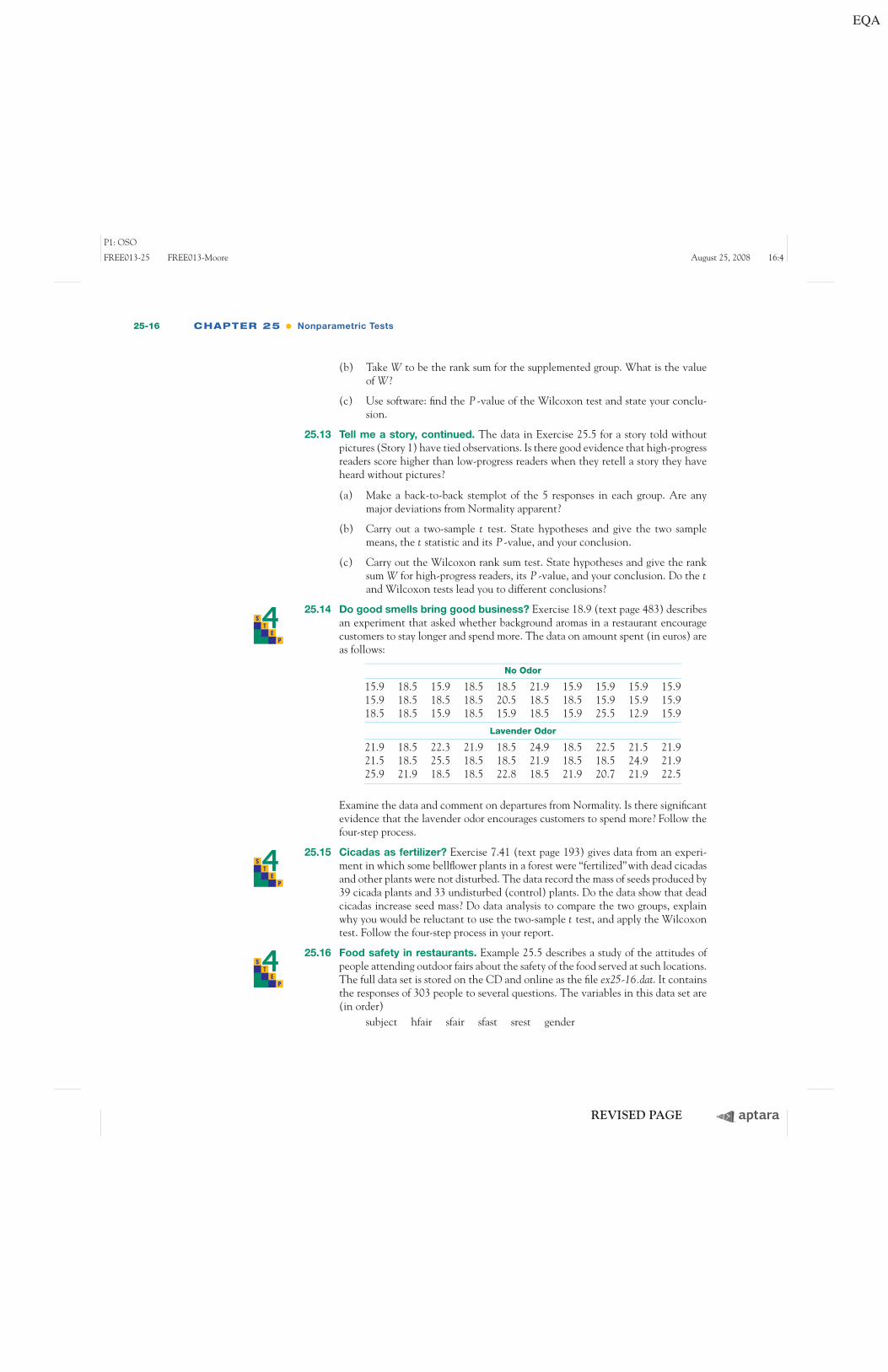
25.14 Do good smells bring good business? Exercise 18.9 (text page 483) describesS
TE
P
an experiment that asked whether background aromas in a restaurant encouragecustomers to stay longer and spend more. The data on amount spent (in euros) areas follows:
Examine the data and comment on departures from Normality. Is there significantevidence that the lavender odor encourages customers to spend more? Follow thefour-step process.
25.15 Cicadas as fertilizer? Exercise 7.41 (text page 193) gives data from an experi-S
TE
P
ment in which some bellflower plants in a forest were “fertilized”with dead cicadasand other plants were not disturbed. The data record the mass of seeds produced by39 cicada plants and 33 undisturbed (control) plants. Do the data show that deadcicadas increase seed mass? Do data analysis to compare the two groups, explainwhy you would be reluctant to use the two-sample t test, and apply the Wilcoxontest. Follow the four-step process in your report.
25.16 Food safety in restaurants. Example 25.5 describes a study of the attitudes ofS
TE
P
people attending outdoor fairs about the safety of the food served at such locations.The full data set is stored on the CD and online as the file ex25-16.dat. It containsthe responses of 303 people to several questions. The variables in this data set are(in order)
subject hfair sfair sfast srest gender
P1: OSO
FREE013-25 FREE013-Moore August 25, 2008 16:4
REVISED PAGE
• Matched pairs: the Wilcoxon signed rank test 25-17
The variable “sfair” contains the responses described in the example concerningsafety of food served at outdoor fairs and festivals. The variable “srest” containsresponses to the same question asked about food served in restaurants. The variable“gender” contains F if the respondent is a woman, M if he is a man. We saw thatwomen are more concerned than men about the safety of food served at fairs. Isthis also true for restaurants? Follow the four-step process in your answer.
25.17 More on food safety. The data file used in Exercise 25.16 contains 303 rows, onefor each of the 303 respondents. Each row contains the responses of one person toseveral questions. We wonder if people are more concerned about safety of foodserved at fairs than they are about the safety of food served at restaurants. Explaincarefully why we cannot answer this question by applying the Wilcoxon rank sumtest to the variables “sfair” and “srest.”
Matched pairs: the Wilcoxon signed
rank test
We use the one-sample t procedures (Chapter 17) for inference about the meanof one population or for inference about the mean difference in a matched pairssetting. The matched pairs setting is more important because good studies are gen-erally comparative. We will now meet a rank test for this setting.
ST
EP
Tell me a storyE X A M P L E 25.6
STATE: A study of early childhood education asked kindergarten students to tell fairytales that had been read to them earlier in the week. Each child told two stories. The firsthad been read to them and the second had been read but also illustrated with pictures.An expert listened to a recording of the children and assigned a score for certain usesof language. Here are the data for five low-progress readers in a pilot study:
We wonder if illustrations improve how the children retell a story.
PLAN: We would like to test the hypotheses
H0: scores have the same distribution for both storiesHa : scores are systematically higher for Story 2
SOLVE (first steps): Because this is a matched pairs design, we base our inference onthe differences. The matched pairs t test gives t = 0.635 with one-sided P -value P =0.280. We cannot assess Normality from so few observations. We would therefore liketo use a rank test. ■
P1: OSO
FREE013-25 FREE013-Moore August 25, 2008 16:4
REVISED PAGE
25-18 CHAPTER 25 • Nonparametric Tests
Positive differences in Example 25.6 indicate that the child performed bettertelling Story 2. If scores are generally higher with illustrations, the positive dif-ferences should be farther from zero in the positive direction than the negativedifferences are in the negative direction. We therefore compare the absolute val-absolute value
ues of the differences, that is, their magnitudes without a sign. Here they are, withboldface indicating the positive values:
0.37 0.23 0.66 0.08 0.17
Arrange these in increasing order and assign ranks, keeping track of which val-ues were originally positive. Tied values receive the average of their ranks. If thereare zero differences, discard them before ranking.
The test statistic is the sum of the ranks of the positive differences. (We could
ST
EP
equally well use the sum of the ranks of the negative differences.) This is theWilcoxon signed rank statistic. Its value here is W+ = 9.
T H E W I L C O X O N S I G N E D R A N K T E S T F O R M A T C H E D P A I R S
Draw an SRS of size n from a population for a matched pairs study and take thedifferences in responses within pairs. Rank the absolute values of these differences.The sum W+ of the ranks for the positive differences is the Wilcoxon signed rankstatistic. If the distribution of the responses is not affected by the different treatmentswithin pairs, then W+ has mean
μW+ = n(n + 1)4
and standard deviation
σW+ =√
n(n + 1)(2n + 1)24
The Wilcoxon signed rank test rejects the hypothesis that there are no systematicdifferences within pairs when the rank sum W+ is far from its mean.
Tell me a story, continuedE X A M P L E 25.7
SOLVE: In the storytelling study of Example 25.6, n = 5. If the null hypothesis (nosystematic effect of illustrations) is true, the mean of the signed rank statistic is
μW+ = n(n + 1)4
= (5)(6)4
= 7.5
P1: OSO
FREE013-25 FREE013-Moore August 25, 2008 16:4
REVISED PAGE
• Matched pairs: the Wilcoxon signed rank test 25-19
The standard deviation of W+ under the null hypothesis is
σW+ =√
n(n + 1)(2n + 1)24
=√
(5)(6)(11)24
=√
13.75 = 3.708
The observed value W+ = 9 is only slightly larger than the mean. We now expect thatthe data are not statistically significant.
The P -value for our one-sided alternative is P (W+ ≥ 9), calculated using thedistribution of W+ when the null hypothesis is true. Software gives the P -valueP = 0.4063.
CONCLUDE: The data give no evidence (P = 0.4) that scores are higher for Story 2. Thedata do show an effect, but it fails to be significant because the sample is very small. ■
A P P L Y Y O U R K N O W L E D G E
25.18 Growing trees faster. Exercise 17.37 (text page 465) describes an experiment inwhich extra carbon dioxide was piped to some plots in a pine forest. Each plot waspaired with a nearby control plot left in its natural state. Do trees grow faster withextra carbon dioxide? Here are the average percent increases in base area for treesin the plots:
Pair Control plot Treated plot
1 9.752 10.5872 7.263 9.2443 5.742 8.675
The investigators used the matched pairs t test. With only 3 pairs, we can’t verifyNormality. We will try the Wilcoxon signed rank test.
(a) Find the differences within pairs, arrange them in order, and rank the abso-lute values. What is the signed rank statistic W+?
(b) If the null hypothesis (no difference in growth) is true, what are the meanand standard deviation of W+? Does comparing W+ to this mean lead to atentative conclusion?
25.19 Fighting cancer. Lymphocytes (white blood cells) play an important role in de-fending our bodies against tumors and infections. Can lymphocytes be geneticallymodified to recognize and destroy cancer cells? In one study of this idea, modifiedcells were infused into 11 patients with metastatic melanoma (serious skin cancer)that had not responded to existing treatments. Here are data for an “ELISA” testfor the presence of cells that trigger an immune response, in counts per 100,000cells before and after infusion.5 High counts suggest that infusion had a beneficialeffect.
(a) Examine the differences (post minus pre). Why can’t we use the matchedpairs t test to see if infusion raised the ELISA counts?
(b) We will apply the Wilcoxon signed rank test. What are the ranks forthe absolute values of the differences in counts? What is the value ofW+?
(c) What would be the mean and standard deviation of W+ if the null hy-pothesis (infusion makes no difference) were true? Compare W+ with thismean (in standard deviation units) to reach a tentative conclusion aboutsignificance.
The Normal approximation for W+
The distribution of the signed rank statistic when the null hypothesis (no differ-ence) is true becomes approximately Normal as the sample size becomes large. Wecan then use Normal probability calculations (with the continuity correction) toobtain approximate P -values for W+. Let’s see how this works in the storytellingexample, even though n = 5 is certainly not a large sample.
Tell me a story: Normal approximationE X A M P L E 25.8
For n = 5 observations, we saw in Example 25.7 that μW+ = 7.5 and that σW+ = 3.708.We observed W+ = 9, so the one-sided P -value is P (W+ ≥ 9). The continuity cor-rection calculates this as P (W+ ≥ 8.5), treating the value W+ = 9 as occupying theinterval from 8.5 to 9.5. We find the Normal approximation for the P -value either fromsoftware or by standardizing and using the standard Normal table:
P (W+ ≥ 8.5) = P(
W+ − 7.53.708
≥ 8.5 − 7.53.708
)
= P (Z ≥ 0.27)
= 0.394 ■
Figure 25.5 displays the output of two statistical programs. Minitab uses theNormal approximation and agrees with our calculation P = 0.394. We askedCrunchIt! to do two analyses: using the exact distribution of W+ and using thematched pairs t test. The exact one-sided P -value for the Wilcoxon signed ranktest is P = 0.4063, as we reported in Example 25.7. The Normal approximationis quite close to this. The t test result is a bit different, P = 0.28, but all threetests tell us that this very small sample gives no evidence that seeing illustrationsimproves the storytelling of low-progress readers.
P1: OSO
FREE013-25 FREE013-Moore August 25, 2008 16:4
REVISED PAGE
• The Normal approximation for W+ 25-21
Minitab
CrunchIt!
HA : Parameter > 0
H0 : Parameter = 0
Parameter : median of Variable
Diff 5 5 9.0 0.394 0.1000
HA : µ1 - µ2 > 0
H0 : µ1 - µ2 = 0
µ1 - µ2 : mean of the paired difference between Story 2 and Story 1
Hypothesis test results:
Hypothesis test results:
Wilcoxon Signed Rank Test: Diff
Diff 5 5 0.1 9 0.4063
Variable n for test Median Est. Wilcoxon Stat. P-value
Exact
Methodn
Story 2 - Story 1 0.11 0.17323394 4 0.6349795 0.28
Test of Median = 0.000000 versus median > 0.000000
N
N Test Statistic P Median
for Wilcoxon Estimated
MINITAB
Wilcoxon Signed Ranks
Paired T statistics
FIGURE 25.5
Output from Minitab and CrunchIt!for the storytelling data of Exam-ple 25.6. The CrunchIt! output com-pares the Wilcoxon signed rank test(with the exact distribution) and thematched pairs t test.
A P P L Y Y O U R K N O W L E D G E
25.20 Growing trees faster: Normal approximation. Continue your work from Exer-cise 25.18. Use the Normal approximation with continuity correction to find theP -value for the signed rank test against the one-sided alternative that trees growfaster with added carbon dioxide. What do you conclude?
P1: OSO
FREE013-25 FREE013-Moore September 9, 2008 13:51
CONFIRMING
25-22 CHAPTER 25 • Nonparametric Tests
25.21 W+ versus t . Find the one-sided P -value for the matched pairs t test applied tothe tree growth data in Exercise 25.18. The smaller P -value of t relative to W+
means that t gives stronger evidence of the effect of carbon dioxide on growth.The t test takes advantage of assuming that the data are Normal, a considerableadvantage for these very small samples.
25.22 Fighting cancer: Normal approximation. Use the Normal approximationwith continuity correction to find the P -value for the test in Exercise 25.19.What do you conclude about the effect of infusing modified cells on the ELISAcount?
David Sanger Photography/Alamy
25.23 Ancient air. Exercise 17.7 (text page 449) reports the following data on the percentof nitrogen in bubbles of ancient air trapped in amber:
63.4 65.0 64.4 63.3 54.8 64.5 60.8 49.1 51.0
We wonder if ancient air differs significantly from the present atmosphere, whichis 78.1% nitrogen.
(a) Graph the data, and comment on skewness and outliers. A rank test is ap-propriate.
John Cumming/Digital Vision/Getty Images
(b) We would like to test hypotheses about the median percent of nitrogen inancient air (the population):
H0 : median = 78.1Ha : median �= 78.1
To do this, apply the Wilcoxon signed rank statistic to the differences be-tween the observations and 78.1. (This is the one-sample version of the test.)What do you conclude?
Dealing with ties in the signed rank test
Ties among the absolute differences are handled by assigning average ranks. Atie within a pair creates a difference of zero. Because these are neither positivenor negative, we drop such pairs from our sample. Ties within pairs simply reducethe number of observations, but ties among the absolute differences complicatefinding a P -value. There is no longer a usable exact distribution for the signedrank statistic W+, and the standard deviation σW+ must be adjusted for the ties
ST
EP
before we can use the Normal approximation. Software will do this. Here is anexample.
Golf scoresE X A M P L E 25.9
STATE: Here are the golf scores of 12 members of a college women’s golf team in tworounds of tournament play. (A golf score is the number of strokes required to completethe course, so that low scores are better.)
Negative differences indicate better (lower) scores on the second round. Based on thissample, can we conclude that this team’s golfers performed differently in the two roundsof a tournament?
PLAN: We would like to test the hypotheses that in a tournament play
H0: scores have the same distribution in Rounds 1 and 2Ha : scores are systematically lower or higher in Round 2
SOLVE: A stemplot of the differences (Figure 25.6) shows some irregularity and a lowoutlier. We will use the Wilcoxon signed rank test.
−1 −1 −0 −0 0 0
6
5 5 5 63 1 2 3 45 5
FIGURE 25.6
Stemplot (with split stems) of thedifferences in scores for two roundsof a golf tournament, forExample 25.9.
Figure 25.7 displays CrunchIt! output for the golf score data. The Wilcoxon statis-tic is W+ = 50.5 with two-sided P -value P = 0.3843. The output also includes thematched pairs t test, for which P = 0.3716. The two P -values are once again similar.
CONCLUDE: These data give no evidence for a systematic change in scores betweenrounds. ■
Paired T statistics
Wilcoxon Signed RanksFIGURE 25.7
Output from CrunchIt! for the golfscores data of Example 25.9. Becausethere are ties, a Normal approxima-tion must be used for the Wilcoxonsigned rank test.
P1: OSO
FREE013-25 FREE013-Moore August 25, 2008 16:4
REVISED PAGE
25-24 CHAPTER 25 • Nonparametric Tests
Let’s see where the value W+ = 50.5 came from. The absolute values of thedifferences, with boldface indicating those that were negative, are
5 5 2 6 5 5 5 16 4 3 3 1
Arrange these in increasing order and assign ranks, keeping track of which val-ues were originally negative. Tied values receive the average of their ranks.
The Wilcoxon signed rank statistic is the sum W+ = 50.5 of the ranks of thenegative differences. (We could equally well use the sum for the ranks of the pos-itive differences.)
A P P L Y Y O U R K N O W L E D G E
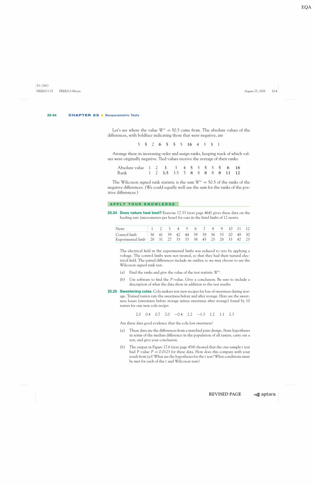
25.24 Does nature heal best? Exercise 17.33 (text page 464) gives these data on thehealing rate (micrometers per hour) for cuts in the hind limbs of 12 newts:
The electrical field in the experimental limbs was reduced to zero by applying avoltage. The control limbs were not treated, so that they had their natural elec-trical field. The paired differences include an outlier, so we may choose to use theWilcoxon signed rank test.
(a) Find the ranks and give the value of the test statistic W+.
(b) Use software to find the P -value. Give a conclusion. Be sure to include adescription of what the data show in addition to the test results.
25.25 Sweetening colas. Cola makers test new recipes for loss of sweetness during stor-age. Trained tasters rate the sweetness before and after storage. Here are the sweet-ness losses (sweetness before storage minus sweetness after storage) found by 10tasters for one new cola recipe:
2.0 0.4 0.7 2.0 −0.4 2.2 −1.3 1.2 1.1 2.3
Are these data good evidence that the cola lost sweetness?
(a) These data are the differences from a matched pairs design. State hypothesesin terms of the median difference in the population of all tasters, carry out atest, and give your conclusion.
(b) The output in Figure 17.6 (text page 454) showed that the one-sample t testhad P -value P = 0.0123 for these data. How does this compare with yourresult from (a)? What are the hypotheses for the t test? What conditions mustbe met for each of the t and Wilcoxon tests?
P1: OSO
FREE013-25 FREE013-Moore August 25, 2008 16:4
REVISED PAGE
• Comparing several samples: the Kruskal-Wallis test 25-25
25.26 Fungus in the air. The air in poultry-processing plants often contains fungusS
TE
P
spores. Inadequate ventilation can damage the health of the workers. The problemis most serious during the summer. To measure the presence of spores, air samplesare pumped to an agar plate, and “colony-forming units (CFUs)” are counted afteran incubation period. Here are data from two locations in a plant that processes37,000 turkeys per day, taken on four days in the summer. The units are CFUs percubic meter of air.6
Spore counts are clearly much higher in the kill room, but with only 4 pairs ofobservations, the difference may not be statistically significant. Apply a rank test.
Comparing several samples: the
Kruskal-Wallis test
We have now considered alternatives to the paired-sample and two-sample ttests for comparing the magnitude of responses to two treatments. To comparemean responses for more than two treatments, we use one-way analysis of vari-ance (ANOVA) if the distributions of the responses to each treatment are at leastroughly Normal and have similar spreads. What can we do when these distribution
ST
EP
requirements are violated?
Weeds among the cornE X A M P L E 25.10
STATE: Lamb’s-quarter is a common weed that interferes with the growth of corn. Aresearcher planted corn at the same rate in 16 small plots of ground, then randomlyassigned the plots to four groups. He weeded the plots by hand to allow a fixed numberof lamb’s-quarter plants to grow in each meter of corn row. These numbers were 0, 1,3, and 9 in the four groups of plots. No other weeds were allowed to grow, and all plotsreceived identical treatment except for the weeds. Here are the yields of corn (bushelsper acre) in each of the plots:7
Weeds Corn Weeds Corn Weeds Corn Weeds Cornper meter yield per meter yield per meter yield per meter yield
Do yields change as the presence of weeds changes?
PLAN: Do data analysis to see how the yields change. Test the null hypothesis “nodifference in the distribution of yields”against the alternative that the groups do differ.
The mean yields do go down as more weeds are added. ANOVA tests whether thedifferences are statistically significant. Can we safely use ANOVA? Outliers are presentin the yields for 3 and 9 weeds per meter. The outliers explain the differences betweenthe means and the medians. They are the correct yields for their plots, so we cannotremove them. Moreover, the sample standard deviations do not quite satisfy our ruleof thumb for ANOVA that the largest should not exceed twice the smallest. We mayprefer to use a nonparametric test. ■
Hypotheses and conditions for the
Kruskal-Wallis test
The ANOVA F test concerns the means of the several populations representedby our samples. For Example 25.10, the ANOVA hypotheses are
H0 :μ0 = μ1 = μ3 = μ9
Ha : not all four means are equal
For example, μ0 is the mean yield in the population of all corn planted underthe conditions of the experiment with no weeds present. The data should con-sist of four independent random samples from the four populations, all Normallydistributed with the same standard deviation.
The Kruskal-Wallis test is a rank test that can replace the ANOVA F test. Thecondition about data production (independent random samples from each popu-lation) remains important, but we can relax the Normality condition. We assumeonly that the response has a continuous distribution in each population. The hy-potheses tested in our example are
H0 : yields have the same distribution in all groups
Ha : yields are systematically higher in some groups than in others
If all of the population distributions have the same shape (Normal or not), thesehypotheses take a simpler form. The null hypothesis is that all four populationshave the same median yield. The alternative hypothesis is that not all four medianyields are equal. The different standard deviations suggest that the four distribu-tions in Example 25.10 do not all have the same shape.
The Kruskal-Wallis test statistic
Recall the analysis of variance idea: we write the total observed variation in theresponses as the sum of two parts, one measuring variation among the groups (sum
P1: OSO
FREE013-25 FREE013-Moore August 25, 2008 16:4
REVISED PAGE
• The Kruskal-Wallis test statistic 25-27
of squares for groups, SSG) and one measuring variation among individual obser-vations within the same group (sum of squares for error, SSE). The ANOVA Ftest rejects the null hypothesis that the mean responses are equal in all groups ifSSG is large relative to SSE.
The idea of the Kruskal-Wallis rank test is to rank all the responses from allgroups together and then apply one-way ANOVA to the ranks rather than to theoriginal observations. If there are N observations in all, the ranks are always thewhole numbers from 1 to N. The total sum of squares for the ranks is thereforea fixed number no matter what the data are. So we do not need to look at bothSSG and SSE. Although it isn’t obvious without some unpleasant algebra, theKruskal-Wallis test statistic is essentially just SSG for the ranks. We give the for-mula, but you should rely on software to do the arithmetic. When SSG is large,that is evidence that the groups differ.
T H E K R U S K A L - W A L L I S T E S T
Draw independent SRSs of sizes n1, n2, . . . , nI from I populations. There are Nobservations in all. Rank all N observations and let Ri be the sum of the ranks forthe ith sample. The Kruskal-Wallis statistic is
H = 12N(N + 1)
∑ R2i
ni− 3(N + 1)
When the sample sizes ni are large and all I populations have the same continuousdistribution, H has approximately the chi-square distribution with I − 1 degrees offreedom.
The Kruskal-Wallis test rejects the null hypothesis that all populations have thesame distribution when H is large.
We now see that, like the Wilcoxon rank sum statistic, the Kruskal-Wallis statis-tic is based on the sums of the ranks for the groups we are comparing. The moredifferent these sums are, the stronger is the evidence that responses are systemati-cally larger in some groups than in others.
The exact distribution of the Kruskal-Wallis statistic H under the null hypothe-sis depends on all the sample sizes n1 to nI , so tables are awkward. The calculationof the exact distribution is so time-consuming for all but the smallest problemsthat even most statistical software uses the chi-square approximation to obtain P -values. As usual, there is no usable exact distribution when there are ties among
ST
EP
the responses. We again assign average ranks to tied observations.
Weeds among the corn, continuedE X A M P L E 25.11
SOLVE (inference): In Example 25.10, there are I = 4 populations and N = 16 obser-vations. The sample sizes are equal, ni = 4. The 16 observations arranged in increasingorder, with their ranks, are
Referring to the table of chi-square critical points (Table D) with df = 3, we see thatthe P -value lies in the interval 0.10 < P < 0.15.
CONCLUDE: Although this small experiment suggests that more weeds decrease yield, itdoes not provide convincing evidence that weeds have an effect. ■
Figure 25.8 displays the Minitab output for both ANOVA and the Kruskal-Wallis test. Minitab agrees that H = 5.56 and gives P = 0.135. Minitab also givesthe results of an adjustment that makes the chi-square approximation more accu-rate when there are ties. For these data, the adjustment has no practical effect.It would be important if there were many ties. A very lengthy computer calcula-tion shows that the exact P -value is P = 0.1299. The chi-square approximationis quite accurate.
The ANOVA F test gives F = 1.73 with P = 0.213. Although the practicalconclusion is the same, ANOVA and Kruskal-Wallis do not agree closely in thisexample. The rank test is more reliable for these small samples with outliers.
A P P L Y Y O U R K N O W L E D G E
25.27 More rain for California? Exercise 24.30 describes an experiment that examinesthe effect on plant biomass in plots of California grassland randomly assigned toreceive added water in the winter, added water in the spring, or no added water.
P1: OSO
FREE013-25 FREE013-Moore August 25, 2008 16:4
REVISED PAGE
• The Kruskal-Wallis test statistic 25-29
Kruskal-Wallis Test: Yield versus Weeds
One-way ANOVA: Yield versus Weeds
Kruskal-Wallis Test on Yield
* NOTE * One or more small samples
Analysis of Variance for Yield
Weeds0139Overall
SourceWeedsErrorTotal
DF31215
SS340.7785.51126.2
MS113.665.5
F1.73
P0.213
Median169.5163.6157.3162.6
Ave Rank13.18.46.36.38.5
N444416
Z2.24-0.06-1.09-1.09
H = 5.56 DF = 3 P = 0.135H = 5.57 DF = 3 P = 0.134 (adjusted for ties)
Individual 95% CIs For MeanBased on Pooled StDev
StDev5.424.4710.4910.12
Mean170.20162.82161.03157.57
N4444
Level0139
Pooled StDev = 8.09 150 160 170 180
SessionFIGURE 25.8
Minitab output for the corn yield dataof Example 25.10. For comparison,both the Kruskal-Wallis test and one-way ANOVA are shown.
The experiment continued for several years. Here are data for 2004 (mass in gramsper square meter):
The sample sizes are small and the data contain some possible outliers. We willapply a nonparametric test.
(a) Examine the data. Show that the conditions for ANOVA (text page 644)are not met. What appear to be the effects of extra rain in winter or spring?
(b) What hypotheses does ANOVA test? What hypotheses does Kruskal-Wallistest?
(c) What are I , the ni , and N? Arrange the counts in order and assign ranks.
P1: OSO
FREE013-25 FREE013-Moore August 25, 2008 16:4
REVISED PAGE
25-30 CHAPTER 25 • Nonparametric Tests
(d) Calculate the Kruskal-Wallis statistic H. How many degrees of freedomshould you use for the chi-square approximation to its null distribution? Usethe chi-square table to give an approximate P -value. What does the test leadyou to conclude?
25.28 Logging in the rain forest: species richness. Table 24.2 (text page 640) con-tains data comparing the number of trees and number of tree species in plots ofland in a tropical rain forest that had never been logged with similar plots nearbythat had been logged 1 year earlier and 8 years earlier. The third response vari-able is species richness, the number of tree species divided by the number of trees.There are low outliers in the data, and a histogram of the ANOVA residuals showsoutliers as well. Because of lack of Normality and small samples, we may prefer theKruskal-Wallis test.
(a) Make a graph to compare the distributions of richness for the three groups ofplots. Also give the median richness for the three groups.
(b) Use the Kruskal-Wallis test to compare the distributions of richness. Statehypotheses, the test statistic and its P -value, and your conclusions.
25.29 Does polyester decay? Here are the breaking strengths (in pounds) of strips ofS
TE
P
polyester fabric buried in the ground for several lengths of time:8
Breaking strength is a good measure of the extent to which the fabric has decayed.Do a complete analysis that compares the four groups. Give the Kruskal-Wallis testalong with a statement in words of the null and alternative hypotheses.
25.30 Compressing soil. Farmers know that driving heavy equipment on wet soil com-S
TE
P
presses the soil and injures future crops. Table 2.5 (text page 65) gives data onthe “penetrability” of the same soil at three levels of compression. Penetrabilityis a measure of how much resistance plant roots will meet when they try to growthrough the soil. Does penetrability systematically change with the degree of com-pression? Do a complete analysis that includes a test of significance. Include a state-ment in words of your null and alternative hypotheses.
25.31 Food safety. Example 25.5 describes a study of the attitudes of people attendingoutdoor fairs about the safety of the food served at such locations. The full data setis stored on the CD and online as the file ex25-16.dat. It contains the responses of303 people to several questions. The variables in this data set are (in order):
subject hfair sfair sfast srest gender
The variable “sfair” contains responses to the safety question described in Exam-ple 25.5. The variables “srest” and “sfast” contain responses to the same questionasked about food served in restaurants and in fast-food chains. Explain carefullywhy we cannot use the Kruskal-Wallis test to see if there are systematic differencesin perceptions of food safety in these three locations.
P1: OSO
FREE013-25 FREE013-Moore August 25, 2008 16:4
REVISED PAGE
Chapter 25 Summary 25-31
C H A P T E R 2 5 S U M M A R Y
■ Nonparametric tests do not require any specific form for the distributions ofthe populations from which our samples come.
■ Rank tests are nonparametric tests based on the ranks of observations, theirpositions in the list ordered from smallest (rank 1) to largest. Tied observationsreceive the average of their ranks. Use rank tests when the data come fromrandom samples or randomized comparative experiments and the populationshave continuous distributions.
■ The Wilcoxon rank sum test compares two distributions to assess whether onehas systematically larger values than the other. The Wilcoxon test is based onthe Wilcoxon rank sum statistic W, which is the sum of the ranks of oneof the samples. The Wilcoxon test can replace the two-sample t test. Soft-ware may perform the Mann-Whitney test, another form of the Wilcoxontest.
■ P-values for the Wilcoxon test are based on the sampling distribution of therank sum statistic W when the null hypothesis (no difference in distributions)is true. You can find P -values from special tables, software, or a Normal ap-proximation (with continuity correction).
■ The Wilcoxon signed rank test applies to matched pairs studies. It tests thenull hypothesis that there is no systematic difference within pairs against alter-natives that assert a systematic difference (either one-sided or two-sided).
■ The test is based on the Wilcoxon signed rank statistic W+ , which is the sumof the ranks of the positive (or negative) differences when we rank the absolutevalues of the differences. The matched pairs t test is an alternative test in thissetting.
■ P-values for the signed rank test are based on the sampling distribution of W+
when the null hypothesis is true. You can find P -values from special tables,software, or a Normal approximation (with continuity correction).
■ The Kruskal-Wallis test compares several populations on the basis of indepen-dent random samples from each population. This is the one-way analysis ofvariance setting.
■ The null hypothesis for the Kruskal-Wallis test is that the distribution of theresponse variable is the same in all the populations. The alternative hypoth-esis is that responses are systematically larger in some populations than inothers.
■ The Kruskal-Wallis statistic H can be viewed in two ways. It is essentially theresult of applying one-way ANOVA to the ranks of the observations. It is alsoa comparison of the sums of the ranks for the several samples.
■ When the sample sizes are not too small and the null hypothesis is true, theKruskal-Wallis test statistic for comparing I populations has approximately thechi-square distribution with I − 1 degrees of freedom. We use this approximatedistribution to obtain P -values.
P1: OSO
FREE013-25 FREE013-Moore August 25, 2008 16:4
REVISED PAGE
25-32 CHAPTER 25 • Nonparametric Tests
S T A T I S T I C S I N S U M M A R Y
Here are the most important skills you should have acquired from reading thischapter.
A. Ranks1. Assign ranks to a moderate number of observations. Use average ranks if
there are ties among the observations.2. From the ranks, calculate the rank sums when the observations come from
two or several samples.
B. Rank Test Statistics1. Determine which of the rank sum tests is appropriate in a specific problem
setting.2. Calculate the Wilcoxon rank sum W from ranks for two samples, the
Wilcoxon signed rank sum W+ for matched pairs, and the Kruskal-Wallisstatistic H for two or more samples.
3. State the hypotheses tested by each of these statistics in specific problemsettings.
4. Determine when it is appropriate to state the hypotheses for W and H interms of population medians.
C. Rank Tests1. Use software to carry out any of the rank tests. Combine the test with data
description and give a clear statement of findings in specific problem set-tings.
2. Use the Normal approximation with continuity correction to find approx-imate P -values for W and W+. Use a table of chi-square critical values toapproximate the P -value for H.
C H E C K Y O U R S K I L L S
25.32 A study of “road rage” gives randomly selected drivers a test that measures “angry/threatening driving.” You wonder if the scores go down with age. You compare thescores for three age groups: less than 30 years, 30 to 55 years, and over 55 years. Youuse the
(a) Wilcoxon rank sum test.
(b) Wilcoxon signed rank test.
(c) Kruskal-Wallis test.
25.33 You interview college students who have done community service and anothergroup of students who have not. To compare the scores of the two groups on atest of attitude toward people of other races, you use the
(a) Wilcoxon rank sum test.
(b) Wilcoxon signed rank test.
(c) Kruskal-Wallis test.
P1: OSO
FREE013-25 FREE013-Moore August 25, 2008 16:4
REVISED PAGE
Check Your Skills 25-33
25.34 You interview 75 students in their freshman year and again in their senior year. Eachinterview includes a test of knowledge of world affairs. To assess whether there hasbeen a significant change from freshman to senior year, you use the
(a) Wilcoxon rank sum test.
(b) Wilcoxon signed rank test.
(c) Kruskal-Wallis test.
25.35 When some plants are attacked by leaf-eating insects, they release chemical com-pounds that repel the insects. Here are data on emissions of one compound by plantsattacked by leaf bugs and by plants in an undamaged control group:
Control group 14.4 15.2 12.6 11.9 5.1 8.0
Attacked group 10.6 15.3 25.2 19.8 17.1 14.6
The rank sum W for the control group is
(a) 21. (b) 26. (c) 52.
25.36 If there is no difference in emissions between the attacked group and the controlgroup, the mean of W in the previous exercise is
(a) 39. (b) 78. (c) 6.2.
25.37 Suppose that the 12 observations in Exercise 25.35 were
Control group 14.4 15.2 12.6 11.9 5.1 8.0
Attacked group 12.6 15.3 25.2 19.8 17.1 14.4
The rank sum for the control group is now
(a) 21. (b) 25. (c) 26.
25.38 Interview 10 young married couples, wife and husband separately. One questionasks how important the attractiveness of their spouse is to them on a scale of 1 to10. Here are the responses:
The Wilcoxon signed rank statistic W+ (based on husband’s score minus wife’sscore) is now
(a) 35. (b) 36. (c) 52.
25.41 You compare the incomes of 4 college freshmen, 5 sophomores, 6 juniors, and 7seniors. If the four income distributions are the same, the Kruskal-Wallis statisticH has approximately a chi-square distribution. The degrees of freedom are
(a) 3. (b) 4. (c) 18.
C H A P T E R 2 5 E X E R C I S E S
One of the rank tests discussed in this chapter is appropriate for each of the following exercises.Follow the Plan, Solve, and Conclude parts of the four-step process in your answers.
25.42 Each day I am getting better in math. Table 18.3 (text page 499) gives theS
TE
P
pretest and posttest scores for two groups of students taking a program to improvetheir basic mathematics skills. Did the treatment group show significantly greaterimprovement than the control group?
25.43 Which blue is most blue? The color of a fabric depends on the dye used and alsoS
TE
P
on how the dye is applied. This matters to clothing manufacturers, who want thecolor of the fabric to be just right. Dye fabric made of ramie with the same “procionblue” die applied in four different ways. Then use a colorimeter to measure thelightness of the color on a scale in which black is 0 and white is 100. Here are thedata for 8 pieces of fabric dyed in each way:9
Method A 41.72 41.83 42.05 41.44 41.27 42.27 41.12 41.49Method B 40.98 40.88 41.30 41.28 41.66 41.50 41.39 41.27Method C 42.30 42.20 42.65 42.43 42.50 42.28 43.13 42.45Method D 41.68 41.65 42.30 42.04 42.25 41.99 41.72 41.97
Do the methods differ in color lightness?
25.44 Right versus left. Table 17.5 (text page 469) contains data from a student projectS
TE
P
that investigated whether right-handed people can turn a knob faster clockwisethan they can counterclockwise. We expect that right-handed people work morequickly when they turn the knob clockwise.
25.45 Logging in the rain forest. Investigators compared the number of tree speciesS
TE
P
in unlogged plots in the rain forest of Borneo with the number of species in plotslogged 8 years earlier. Here are the data:10
Unlogged 22 18 22 20 15 21 13 13 19 13 19 15
Logged 17 4 18 14 18 15 15 10 12
Does logging significantly reduce the number of species in a plot after 8 years?
P1: OSO
FREE013-25 FREE013-Moore August 25, 2008 16:4
REVISED PAGE
Chapter 25 Exercises 25-35
25.46 Food safety at fairs and restaurants. Example 25.5 describes a study of theS
TE
P
attitudes of people attending outdoor fairs about the safety of the food served atsuch locations. The full data set is stored on the CD and online as the file ex25-16.dat. It contains the responses of 303 people to several questions. The variablesin this data set are (in order)
subject hfair sfair sfast srest gender
The variable “sfair” contains responses to the safety question described in Example25.5. The variable “srest”contains responses to the same question asked about foodserved in restaurants. We suspect that restaurant food will appear safer than foodserved outdoors at a fair. Do the data give good evidence for this suspicion?
25.47 Food safety at fairs and fast-food restaurants. The food safety survey dataS
TE
P
described in Example 25.5 also contain the responses of the 303 subjects tothe same question asked about food served at fast-food restaurants. These re-sponses are the values of the variable “sfast.” Is there a systematic difference be-tween the level of concern about food safety at outdoor fairs and at fast-foodrestaurants?
25.48 Nematodes and plant growth. A botanist prepares 16 identical planting potsS
TE
P
and then introduces different numbers of nematodes (microscopic worms) into thepots. A tomato seedling is transplanted into each pot. Here are data on the increasein height of the seedlings (in centimeters) 16 days after planting:11
25.49 Mutual fund performance. Mutual funds often compare their performance withS
TE
P
a benchmark provided by an “index” that describes the performance of the class ofassets in which the funds invest. For example, the Vanguard International GrowthFund benchmarks its performance against the EAFE (Europe, Australasia, Far East)index. Table 17.4 (text page 468) gives the annual returns (percent) for the fundand the index. Does the fund’s performance differ significantly from that of itsbenchmark?
How does the meeting of large rivers influence the diversity of fish? A study of the Amazon and 13of its major tributaries concentrated on electric fish, which are common in South America. Theresearchers trawled in more than 1000 locations in the Amazon above and below each tributaryand in the lower part of the tributaries themselves. In all, they found 43 species of electric fish.These distinctive fish can “stand in”for fish in general, which are too numerous to count easily. Theresearchers concluded that the number of fish species increases when a tributary joins the Amazon,but that the effect is local: there is no steady increase in diversity as we move downstream. Table25.1 gives the estimated number of electric fish species in the Amazon upstream and downstreamfrom each tributary and in the tributaries themselves just before they flow into the Amazon.12 Theresearchers used nonparametric tests to assess the statistical significance of their results. Exercises25.50 to 25.52 quote conclusions from the study.
25.50 Downstream versus upstream. “We identified a significant positive effect oftributaries on Amazon mainstem species richness in two respects. First, we foundthat sample stations downstream of each tributary contained more species than didtheir respective upstream stations.” Do a test to confirm the statistical significanceof this effect and report your conclusion.
25.51 Tributary versus upstream. “Second, we found that species richness within trib-utaries exceeded that within their adjacent upstream mainstem stations.”Again, doa test to confirm significance and report your finding.
25.52 Tributary versus downstream. Species richness “was comparable between tribu-taries and their adjacent downstream mainstem stations.”Verify this conclusion bycomparing tributary and downstream species counts.
N O T E S A N D D A T A S O U R C E S
1. Data provided by Samuel Phillips, Purdue University.
2. Data provided by Susan Stadler, Purdue University.
3. The precise meaning of “yields are systematically larger in plots with noweeds” is that for every fixed value a , the probability that the yield with noweeds is larger than a is at least as great as the same probability for the yieldwith weeds.
4. Huey Chern Boo, “Consumers’ perceptions and concerns about safety andhealthfulness of food served at fairs and festivals,”MS thesis, Purdue Univer-sity, 1997.
5. Richard A. Morgan et al., “Cancer regression in patients after transfer ofgenetically engineered lymphocytes,”Science, 314 (2006), pp. 126–129. Thedata appear in the Online Supplementary Material.
P1: OSO
FREE013-25 FREE013-Moore August 25, 2008 16:4
REVISED PAGE
Notes and Data Sources 25-37
6. Michael W. Peugh, “Field investigation of ventilation and air quality in duckand turkey slaughter plants,” MS thesis, Purdue University, 1996.
7. See Note 1.
8. Sapna Aneja, “Biodeterioration of textile fibers in soil,” MS thesis, PurdueUniversity, 1994.
9. Yvan R. Germain, “The dyeing of ramie with fiber reactive dyes using thecold pad-batch method,” MS thesis, Purdue University, 1988.
10. I thank Charles Cannon of Duke University for providing the data. The studyreport is C. H. Cannon, D. R. Peart, and M. Leighton, “Tree species diversityin commercially logged Bornean rainforest,” Science, 281 (1998), pp. 1366–1367.
11. Data provided by Matthew Moore.
12. Cristina Cox Fernandes, Jeffrey Podos, and John G. Lundberg, “Amazonianecology: tributaries enhance the diversity of electric fishes,” Science, 305(2004), pp. 1960–1962.