Chapter 3 Coulomb collisions Coulomb collisions are long-range scattering events between charged particles due to the mutual exchange of the Coulomb force. Where do they occur, and why they are of interest? • energy redistribution among particles of the same species or between di↵erent species – equilibrium vs non equilibrium – fluid description vs kinetic description • slowing-down of fast particles (e.g. charged fusion products, externally injected energetic particles) • transport processes (e.g. thermal conduction, viscosity) • electric resistivity • emission and absorption of radiation Most relevant di↵erences with respect to collisions in a gas • “continous” and “simultaneous”: how do we define mean free path, collision frequency, etc.?
Transcript
Chapter 3
Coulomb collisions
Coulomb collisions are long-range scattering events between charged particles due
to the mutual exchange of the Coulomb force.
Where do they occur, and why they are of interest?
• energy redistribution among particles of the same species or between di↵erent
species
– equilibrium vs non equilibrium
– fluid description vs kinetic description
• slowing-down of fast particles (e.g. charged fusion products, externally injected
energetic particles)
• transport processes (e.g. thermal conduction, viscosity)
• electric resistivity
• emission and absorption of radiation
Most relevant di↵erences with respect to collisions in a gas
• “continous” and “simultaneous”: how do we define mean free path, collision
frequency, etc.?
3
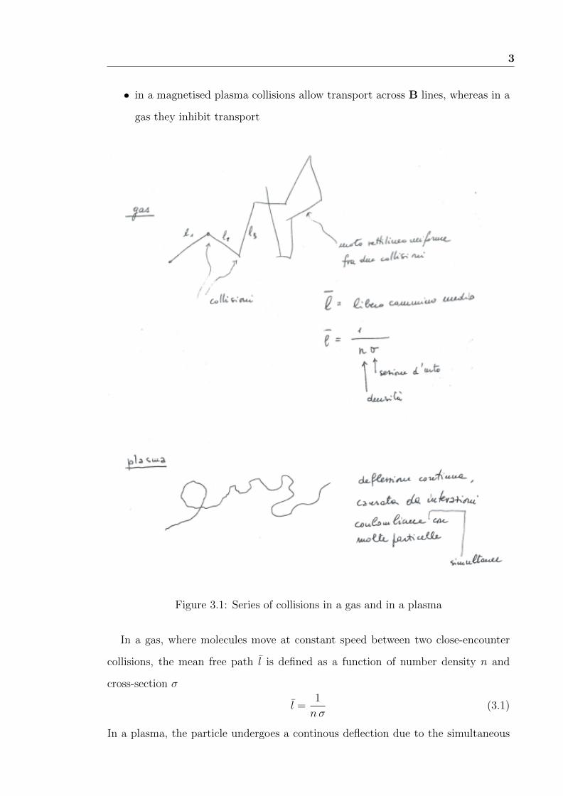
• in a magnetised plasma collisions allow transport across B lines, whereas in a
gas they inhibit transport
Figure 3.1: Series of collisions in a gas and in a plasma
In a gas, where molecules move at constant speed between two close-encounter
collisions, the mean free path l is defined as a function of number density n and
cross-section �
l =1
n �(3.1)
In a plasma, the particle undergoes a continous deflection due to the simultaneous
4
Coulomb interaction with many particles. As such, we cannot define the mean free
path in the same way as Eq. 3.1, but we define an e↵ective mean free path as the
average distance travelled by particle ending with a 90o deflection with respect to
the original direction.
In this chapter we will present a simplified description, which anyhow is able to
reproduce all the correct functional dependencies and scaling laws.
For rigorous and in-depth description of Coulomb collisions in a plasma please refer
to:
• Sivukhin, D.V. (1966), “Coulomb collisions in fully ionized plasma” in Review
of Plasma Physics (ed. A,M. Leontovich), IV, 93-241, Consultants Bureau,
New York.
• a detailed description of Rutherford cross-section can be found, for instance,
in:
– L. Landau and E. Lifshitz, Fisica Teorica, vol. 1 - Meccanica, §19, Ed.
Mir, Moscow (1982)
– M. Bertolotti, T. Papa, D. Sette, Guida alla soluzione di problemi di fisica
II, Ed. Veschi/Masson, p. 156
• it can be shown that the classical derivation presented in these notes agrees
with the quantum mechanical approach: see e.g.
– L. Landau and E. Lifshitz, Fisica Teorica, vol. 3 - Meccanica Quantistica,
§135, p. 655, Ed. Riuniti (1976)
3.1 Single binary collision 5
3.1 Single binary collision
Scattering of a projectile particle P o↵ a target particle F .
We recall that in an elastic collision the modulus of the relative velocity is conserved,
so that in the centre of mass frame we have a deflection only (see Appenix A).
projectile
Figure 3.2: binary Coulomb collision
Here F is a fixed scattering centre, i.e. its mass M ! 1. The obtained results
can be extended to the general case of finite mass M by substitution of projectile
mass m with the reduced mass mr
= mM/(m+M), and by changing the projectile
velocity v with the relative velocity vr
.
Particle trajectory is a hyperbola, with focus F and
✓ = scattering angle
↵ = angle between hyperbola axis and asymptote
b = impact parameter
3.1 Single binary collision 6
� = minimum approach distance between projectile and target
Recalling the geometric properties of a hyperbola, we can state
� = FA = b cot↵
2(3.2)
angular momentum conservation with respect to F
b v = � vA
) vA
= v tan↵
2(3.3)
energy conservation between P (t = �1) and A
1
2mv2 =
1
2mv2
A
+qQ
4⇡"0
�) v2
A
= v2 �2qQ
4⇡"0
�m(3.4)
) v2A
= v2 �b0
�v2 ) v2
A
= v2✓1�
b0
btan
↵
2
◆(3.5)
where
b0
=2qQ
4⇡"0
1
mv2(3.6)
Inserting Eq.3.3 in 3.5 we obtain
v2 tan2
↵
2= v2
✓1�
b0
btan
↵
2
◆) 1� tan2
↵
2=
b0
btan
↵
2(3.7)
cos2 ↵
2
� sin2 ↵
2
cos2 ↵
2
=b0
b
sin ↵
2
cos ↵
2
)
cos↵
cos ↵
2
=b0
bsin
↵
2)
tan↵ =2b
b0
(3.8)
It can be seen in Fig.3.4 that ↵ = (⇡ � ✓)/2, hence tan↵ = cot ✓/2, and Eq.3.8
becomes
tan✓
2=
b0
2b=
qQ
4⇡"0
1
mv2 b(3.9)
See Appendix C for a relation between this last equation and Rutherford cross-
section.
3.1 Single binary collision 7
3.1.1 Meaning of b0 parameter (Landau distance)
Let’s simply rewrite Eq.3.6 in this way
b0
=qQ
4⇡"0
�mv2
2, (3.10)
which cleary indicates that b0
is the distance at which the initial kinetic energy of
the projectile is equal to the electrostatic potential energy. The projectile can reach
this distance in the case of head-on collision only, when the impact parameter b is
zero.
Figure 3.3: Scattering angle as a function of impact parameter
• for a given b, collisions become “harder” with increasing b0
• for the general formula, make the substitution mv2 ! mr
v2r
• small-deflection collisions are much more frequent than large-deflection colli-
sions (dn / b db).
• we can arbritrarily define a threshold and distinghish collisions in
b < b0
: large-deflection collisions
b > b0
: small-deflection collisions
3.1 Single binary collision 8
• a quantum mechanical approach indicates that we should replace
b0
! max(b0
,�deBroglie
)
• also the plasma screening implies that a particle interacts via the Coulomb
force only with particles within its Debye sphere, so that b < �D
Large-angle deflections in an ideal plasma are typically the result of a series of small-
angle deflections. Let ⌫c
be the frequency of large-angle deflection as a result of many
small-angle deflections. Let ⌫cr
be the frequency of large-angle deflection as a result
of a single deflection. Then it can be shown (see, e.g., Pucella-Segre, pp. 40-42) that
⌫c
⌫cr
= 2 ln�D
bmin
= 2 ln⇤ , (3.11)
where the Coulomb logarithm ln⇤ (see hereafter) is typically in the range 10-
20. Hence the main contribution comes from collisions with small-angle deflection,
whereas hard Coulomb collisions are rare events with respect to these.
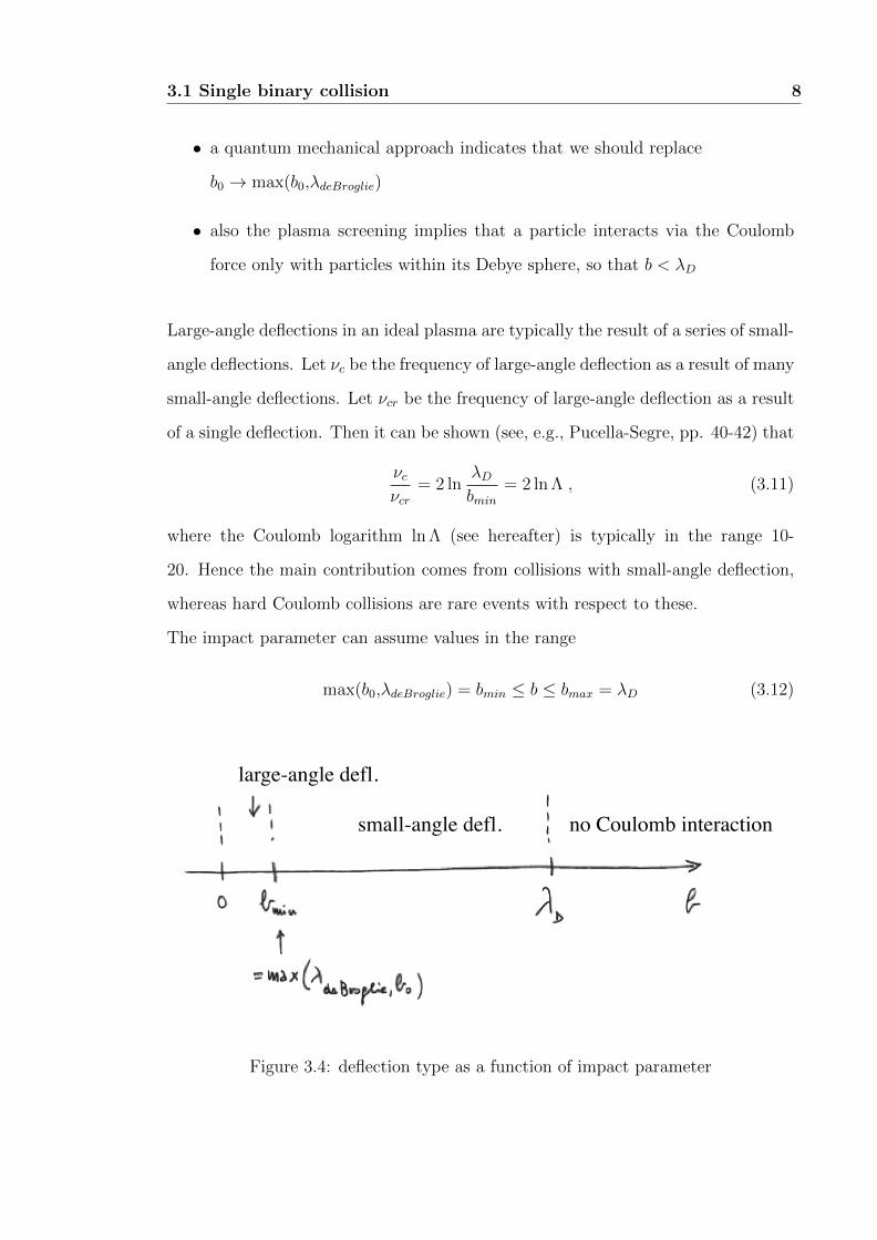
The impact parameter can assume values in the range
max(b0
,�deBroglie
) = bmin
b bmax
= �D
(3.12)
large-angle defl.
small-angle defl. no Coulomb interaction
Figure 3.4: deflection type as a function of impact parameter
3.2 Simultaneous multiple collisions in a plasma 9
3.2 Simultaneous multiple collisions in a plasma
Let’s study the cumulative e↵ect of many Coulomb collisions in the small-angle
regime.
In small angle approximation, Eq. 3.9 becomes
tan✓
2'
✓
2=
b0
2b) ✓ '
b0
b(3.13)
the variation of v in the perpendicular direction is therefore
|�v?| = �v? ' v✓ ' vb0
b(3.14)
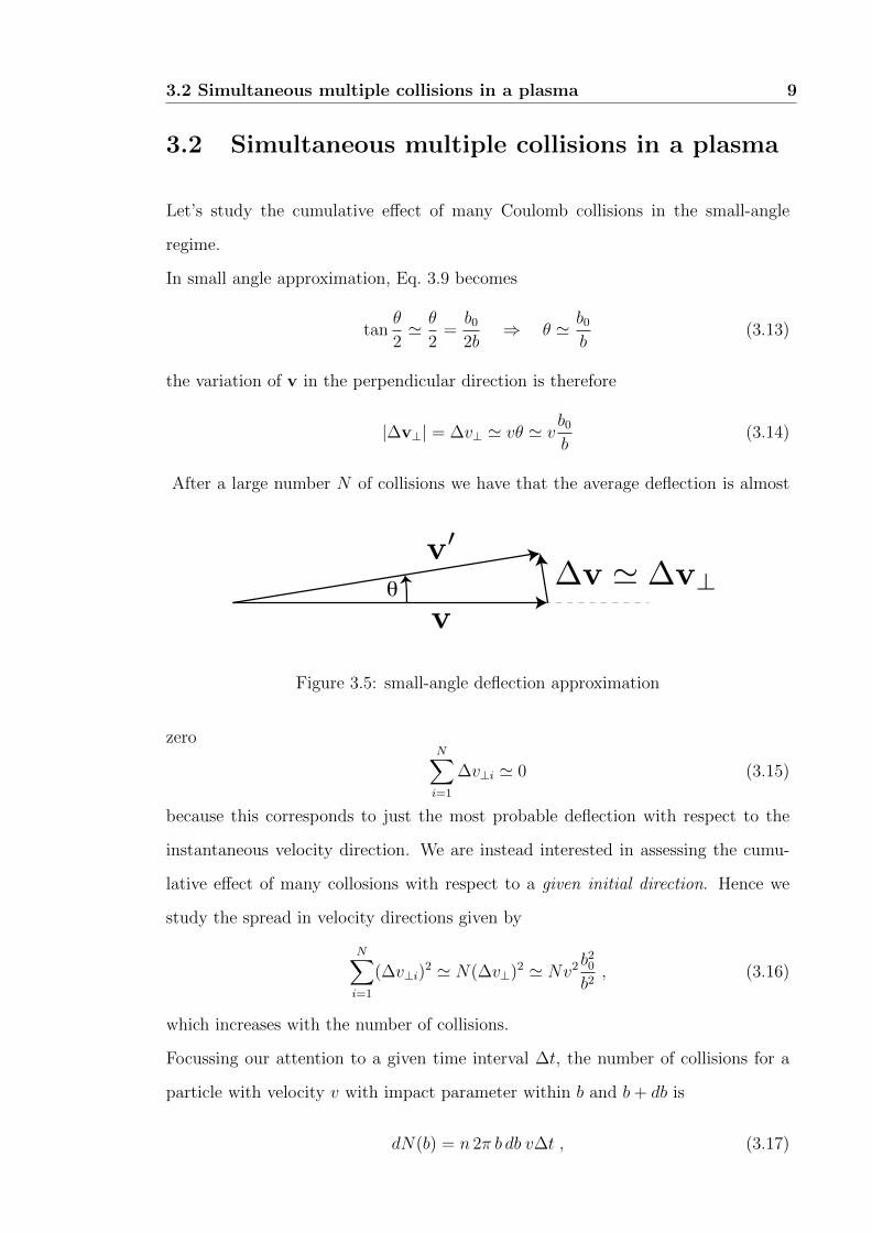
After a large number N of collisions we have that the average deflection is almost
θ
Figure 3.5: small-angle deflection approximation
zeroNX
i=1
�v?i
' 0 (3.15)
because this corresponds to just the most probable deflection with respect to the
instantaneous velocity direction. We are instead interested in assessing the cumu-
lative e↵ect of many collosions with respect to a given initial direction. Hence we
study the spread in velocity directions given by
NX
i=1
(�v?i
)2 ' N(�v?)2
' Nv2b20
b2, (3.16)
which increases with the number of collisions.
Focussing our attention to a given time interval �t, the number of collisions for a
particle with velocity v with impact parameter within b and b+ db is
dN(b) = n 2⇡ b db v�t , (3.17)
3.2 Simultaneous multiple collisions in a plasma 10
where n is the number density of scattering centres. The corresponding cumulative
velocity spread isNX
i=1
(�v?i
)2 ' n 2⇡ b db v3�tb20
b2, (3.18)
and integrating over all possible impact parameters we obtain
NX
i=1
(�v?i
)2 ' 2⇡ n v3�t b20
Zb
max
b
min
db
b= 2⇡ n v3�t b2
0
lnbmax
bmin
, (3.19)
where ln b
max
b
min
= ln⇤ is the Coulomb logarithm, which depends on several plasma
parameters, but it is anyhow in the range 5 to 20 for the plasmas considered in this
course.
3.2.1 Collision time and collision frequency
We define the collision time ⌧ as the time interval necessary for a particle to be
deflected (on average) by 90o, i.e. when the cumulative spread velocity is of the
order of v2. Hence, using Eq.3.19, we solve for ⌧ in
NX
i=1
(�v?i
)2 ' 2⇡ n v3⌧ b20
ln⇤ ' v2 (3.20)
⌧ = 1.2⇡ n v b2
0
ln⇤ (3.21)
and we obtain the collision frequency ⌫ as
⌫ =1
⌧= 2⇡ n v b2
0
ln⇤ , (3.22)
which can be written using 3.6 as
⌫ =1
2⇡"20
q2 Q2
m2v3n ln⇤ , (3.23)
Let’s rewrite this last equation for the general case of a particle of species ↵ scattering
o↵ particles of species � with number density n�
:
⌫↵�
=1
2⇡"20
q↵
q�
m2
↵�
v3r
n�
ln⇤↵�
, (3.24)
3.2 Simultaneous multiple collisions in a plasma 11
where m↵�
= m↵
m�
/(m↵
+ m�
) is the reduced mass, and vr
is a characteristic
relative velocity for the two considered species.
We will consider in the following the electron-electron collisions, the electron-ion
collisions, and the ion-ion collisions. Table 3.2.1 presents the parameters corres-
ponding the various cases. We assume that the plasma is fully ionised, and that
the two species, ions and electrons, are in thermal equilibrium within themselves, so
that the typical velocities are the respective thermal velocities vth,e
=p
3kB
Te
/me
and vth,i
=p3k
B
Ti
/mi
. In order to estimate the characteristic relative velocity vr
,
we observe that in general ve
� vi
.
For instance, we have
⌫ee
'
1
2⇡"20
e4
m1/2
e
(3kB
Te
)3/2ne
ln⇤ee
(3.25)
' 4,18 · 10�12
ne
[m�3]
(Te
[ eV])3/2ln⇤
ee
Hz (3.26)
' 1,32 · 10�16
ne
[m�3]
(Te
[ keV])3/2ln⇤
ee
Hz (3.27)
⌧ee
=1
⌫ee
' 7,55 · 1015(T
e
[ keV])3/2
ne
[m�3] ln⇤ee
s (3.28)
Table 3.1: typical parameters for the collision frequency for a fully ionised plasma
collision charge m↵�
vr
density
e ! e e4 me
/2 vth,e
ne
= Z ni
e ! i e4Z2 me
vth,e
ni
i ! i e4Z4 mi
/2 vth,i
ni
Comparing the various collision frequencies we can state that
⌫ee
: ⌫ei
: ⌫ii
= Z : Z2 :
rm
e
mi
Z4
✓Te
Ti
◆3/2
(3.29)
so that typically the dominating frequency is the ei collision frequency. In the
special, but very important case, of fully ionised Hydrogen plasma (Z = 1) in
thermal equilibrium (Te
= Ti
) we have
⌫ee
: ⌫ei
: ⌫ii
= 1 : 1 : 1/43 (3.30)
3.2 Simultaneous multiple collisions in a plasma 12
so that ee and ei collisions occur at the same frequency, much larger than the ii
collision frequency.
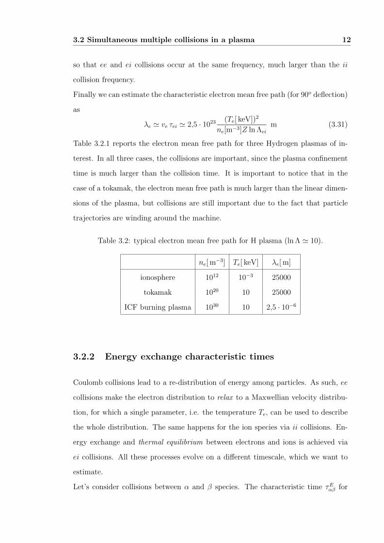
Finally we can estimate the characteristic electron mean free path (for 90o deflection)
as
�e
' ve
⌧ei
' 2,5 · 1023(T
e
[ keV])2
ne
[m�3]Z ln⇤ei
m (3.31)
Table 3.2.1 reports the electron mean free path for three Hydrogen plasmas of in-
terest. In all three cases, the collisions are important, since the plasma confinement
time is much larger than the collision time. It is important to notice that in the
case of a tokamak, the electron mean free path is much larger than the linear dimen-
sions of the plasma, but collisions are still important due to the fact that particle
trajectories are winding around the machine.
Table 3.2: typical electron mean free path for H plasma (ln⇤ ' 10).
ne
[ m�3] Te
[ keV] �e
[ m]
ionosphere 1012 10�3 25000
tokamak 1020 10 25000
ICF burning plasma 1030 10 2,5 · 10�6
3.2.2 Energy exchange characteristic times
Coulomb collisions lead to a re-distribution of energy among particles. As such, ee
collisions make the electron distribution to relax to a Maxwellian velocity distribu-
tion, for which a single parameter, i.e. the temperature Te
, can be used to describe
the whole distribution. The same happens for the ion species via ii collisions. En-
ergy exchange and thermal equilibrium between electrons and ions is achieved via
ei collisions. All these processes evolve on a di↵erent timescale, which we want to
estimate.
Let’s consider collisions between ↵ and � species. The characteristic time ⌧E↵�
for
3.2 Simultaneous multiple collisions in a plasma 13
energy exchange can be defined as
⌧E↵�
' Ncoll
⌧↵�
, (3.32)
where Ncoll
is the number of collision needed to transfer an amount of energy E, and
⌧↵�
is the collision time. From a head-on elastic collision, we can obtain the order
of magnitude of energy transfer in a single collision
<�E>↵�
' �Ehead�on
=4m
↵
/m�
(1 +m↵
/m�
)2E (3.33)
So that Ncoll
' E/ < �E >, and inserting this in Eq.3.32 we obtain
⌧E↵�
' ⌧↵�
(1 +m↵
/m�
)2
4m↵
/m�
(3.34)
The relevant energy exchange times are
⌧Eee
' ⌧ee
=1
⌫ee
(3.35)
⌧Eei
' ⌧ei
mi
4me
=1
⌫ee
mi
4me
(3.36)
⌧Eii
' ⌧ii
=1
⌫ii
(3.37)
Using these equations and Eq.3.29, we have (Te
' Ti
)
⌧Eee
: ⌧Eii
: ⌧Eei
= 1 :1
Z3
rm
i
me
:1
Z
mi
4me
, (3.38)
which typically means that ⌧Eee
⌧ ⌧Eii
⌧ ⌧Eei
. Hence electron and ions relax to
a Maxwellian much faster than they reach thermal equilibrium between the two
species.
In cases where there are heating or cooling processes happening on a timescale ⌧
shorter than ⌧Eei
, but longer than ⌧Eee
and ⌧Eii
, we can consider the plasma as made up
by two species, each one in thermal equilibrium, but having a di↵erent temperature,
i.e. Te
6= Ti
. In this case, we can model the plasma as a single fluid with two
temperatures, and the volumetric rate of energy exchange reads
dEe!i
dt=
3
2
ne
kB
(Te
� Ti
)
⌧Eei
(3.39)
3.2 Simultaneous multiple collisions in a plasma 14
Practical formulas for energy exchange rate are
⌧Eee
' 1,1 · 1016T 3/2
e
[ keV]
ne
[ m3] ln⇤ee
s (3.40)
⌧Eei
' 1019A
Z
T 3/2
e
[ keV]
ne
[ m3] ln⇤ei
s (3.41)
where A is the ion mass number, and Z the atomic number.
Table 3.2.2 compares the thermal equilibrium times for equimolar DT plasma. It
is worthwhile to notice that the equilibrium times are typically longer than other
chacteristic times for these plasmas, so that in several cases we can assume Te
6= Ti
.
Table 3.3: typical thermal equilibrium times for equimolar DT plasma (Z = 1;A =
2,5; ln⇤ ' 10).
⌧Eei
ne
[ m�3] Te
= 1keV Te
= 10 keV
tokamak 1020 0,025 s 0,8 s
mid range density 1026 25 ns 800 ns
ICF burning plasma 1031 0,25 ps 8 ps
3.3 Appendix A: elastic collision properties 15
3.3 Appendix A: elastic collision properties
In an elastic collision the modulus of relative velocity is conserved. Hence in the
CoM frame the elastic collision is just a deflection. Let’s consider two point masses
m1
and m2
moving respectively with velocity v1
and v2
in the laboratory frame.
The kinetic energy of the two colliding masses can be written (Konig theorem)
T =1
2(m
1
+m2
) v2c
+1
2m
1
v21c
+1
2m
2
v22c
, (3.42)
where vc
is the CoM velocity, and v1c
and v2c
the point mass velocities with respect
to the CoM:
vc
=m
1
m1
+m2
v1
+m
2
m1
+m2
v2
(3.43)
v1c
= v1
� vc
=m
2
m1
+m2
(v1
� v2
) =m
2
m1
+m2
vr
(3.44)
v2c
= v2
� vc
=m
1
m1
+m2
(v2
� v1
) = �
m1
m1
+m2
vr
(3.45)
1
2m
1
v21c
+1
2m
2
v22c
=1
2
m1
m2
m1
+m2
m2
m1
+m2
v2r
+1
2
m2
m1
m1
+m2
m1
m1
+m2
v2r
(3.46)
=1
2
m1
m2
m1
+m2
v2r
=1
2m
r
v2r
, (3.47)
where vr
is the relative velocity, andmr
is the reduced mass. Hence Eq. 3.42 becomes
T =1
2(m
1
+m2
) v2c
+1
2m
r
v2r
(3.48)
Since T is conserved (elastic collision), and vc
does not change (internal forces only),
vr
is conserved. Therefore we have a deflection of relative velocity only.
3.4 Appendix B: geometry of Rutherford scattering 16