CHAPTER CPU Scheduling -...

6C H A P T E R

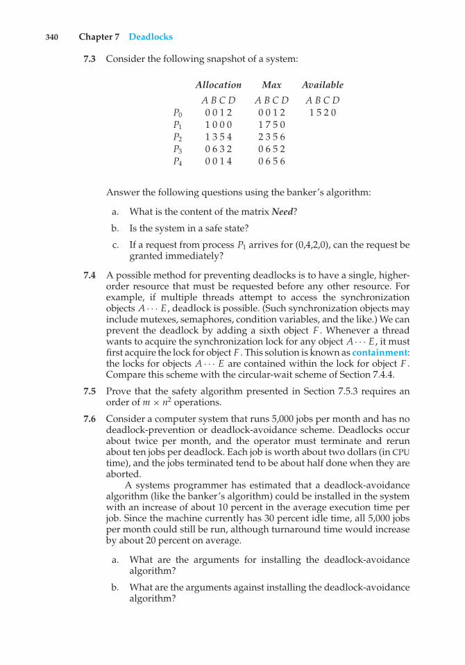
CPUScheduling

CPU scheduling is the basis of multiprogrammed operating systems. Byswitching the CPU among processes, the operating system can make thecomputer more productive. In this chapter, we introduce basic CPU-schedulingconcepts and present several CPU-scheduling algorithms. We also consider theproblem of selecting an algorithm for a particular system.

In Chapter 4, we introduced threads to the process model. On operatingsystems that support them, it is kernel-level threads—not processes—thatare in fact being scheduled by the operating system. However, the terms"process scheduling" and "thread scheduling" are often used interchangeably.In this chapter, we use process scheduling when discussing general schedulingconcepts and thread scheduling to refer to thread-specific ideas.

CHAPTER OBJECTIVES

• To introduce CPU scheduling, which is the basis for multiprogrammedoperating systems.

• To describe various CPU-scheduling algorithms.

• To discuss evaluation criteria for selecting a CPU-scheduling algorithm fora particular system.

• To examine the scheduling algorithms of several operating systems.

6.1 Basic Concepts

In a single-processor system, only one process can run at a time. Othersmust wait until the CPU is free and can be rescheduled. The objective ofmultiprogramming is to have some process running at all times, to maximizeCPU utilization. The idea is relatively simple. A process is executed untilit must wait, typically for the completion of some I/O request. In a simplecomputer system, the CPU then just sits idle. All this waiting time is wasted;no useful work is accomplished. With multiprogramming, we try to use thistime productively. Several processes are kept in memory at one time. When

261

262 Chapter 6 CPU Scheduling

CPU burstload storeadd storeread from file

store incrementindexwrite to file

load storeadd storeread from file

wait for I/O

wait for I/O

wait for I/O

I/O burst

I/O burst

I/O burst

CPU burst

CPU burst

•••

•••

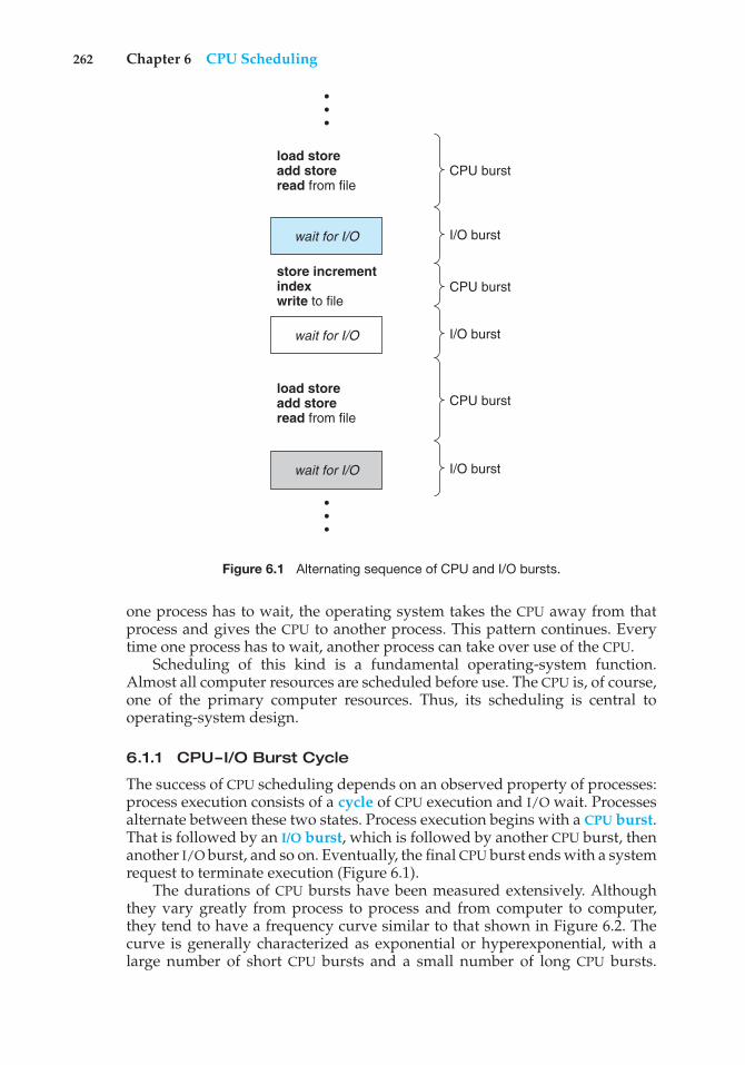
Figure 6.1 Alternating sequence of CPU and I/O bursts.

one process has to wait, the operating system takes the CPU away from thatprocess and gives the CPU to another process. This pattern continues. Everytime one process has to wait, another process can take over use of the CPU.

Scheduling of this kind is a fundamental operating-system function.Almost all computer resources are scheduled before use. The CPU is, of course,one of the primary computer resources. Thus, its scheduling is central tooperating-system design.

6.1.1 CPU–I/O Burst Cycle

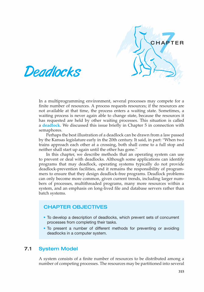
The success of CPU scheduling depends on an observed property of processes:process execution consists of a cycle of CPU execution and I/O wait. Processesalternate between these two states. Process execution begins with a CPU burst.That is followed by an I/O burst, which is followed by another CPU burst, thenanother I/O burst, and so on. Eventually, the final CPU burst ends with a systemrequest to terminate execution (Figure 6.1).

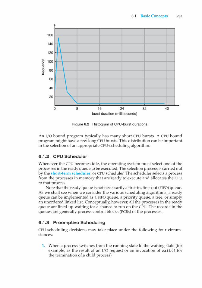
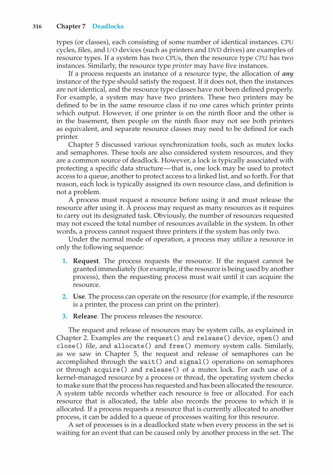
The durations of CPU bursts have been measured extensively. Althoughthey vary greatly from process to process and from computer to computer,they tend to have a frequency curve similar to that shown in Figure 6.2. Thecurve is generally characterized as exponential or hyperexponential, with alarge number of short CPU bursts and a small number of long CPU bursts.

6.1 Basic Concepts 263

freq

uenc

y

160

140

120

100

80

60

40

20

0 8 16 24 32 40burst duration (milliseconds)

Figure 6.2 Histogram of CPU-burst durations.

An I/O-bound program typically has many short CPU bursts. A CPU-boundprogram might have a few long CPU bursts. This distribution can be importantin the selection of an appropriate CPU-scheduling algorithm.

6.1.2 CPU Scheduler

Whenever the CPU becomes idle, the operating system must select one of theprocesses in the ready queue to be executed. The selection process is carried outby the short-term scheduler, or CPU scheduler. The scheduler selects a processfrom the processes in memory that are ready to execute and allocates the CPUto that process.

Note that the ready queue is not necessarily a first-in, first-out (FIFO) queue.As we shall see when we consider the various scheduling algorithms, a readyqueue can be implemented as a FIFO queue, a priority queue, a tree, or simplyan unordered linked list. Conceptually, however, all the processes in the readyqueue are lined up waiting for a chance to run on the CPU. The records in thequeues are generally process control blocks (PCBs) of the processes.

6.1.3 Preemptive Scheduling

CPU-scheduling decisions may take place under the following four circum-stances:

1. When a process switches from the running state to the waiting state (forexample, as the result of an I/O request or an invocation of wait() forthe termination of a child process)


2. When a process switches from the running state to the ready state (forexample, when an interrupt occurs)

3. When a process switches from the waiting state to the ready state (forexample, at completion of I/O)

4. When a process terminates

For situations 1 and 4, there is no choice in terms of scheduling. A new process(if one exists in the ready queue) must be selected for execution. There is achoice, however, for situations 2 and 3.

When scheduling takes place only under circumstances 1 and 4, we saythat the scheduling scheme is nonpreemptive or cooperative. Otherwise,it is preemptive. Under nonpreemptive scheduling, once the CPU has beenallocated to a process, the process keeps the CPU until it releases the CPU eitherby terminating or by switching to the waiting state. This scheduling methodwas used by Microsoft Windows 3.x. Windows 95 introduced preemptivescheduling, and all subsequent versions of Windows operating systems haveused preemptive scheduling. The Mac OS X operating system for the Macintoshalso uses preemptive scheduling; previous versions of the Macintosh operatingsystem relied on cooperative scheduling. Cooperative scheduling is the onlymethod that can be used on certain hardware platforms, because it does notrequire the special hardware (for example, a timer) needed for preemptivescheduling.

Unfortunately, preemptive scheduling can result in race conditions whendata are shared among several processes. Consider the case of two processesthat share data. While one process is updating the data, it is preempted so thatthe second process can run. The second process then tries to read the data,which are in an inconsistent state. This issue was explored in detail in Chapter5.

Preemption also affects the design of the operating-system kernel. Duringthe processing of a system call, the kernel may be busy with an activity on behalfof a process. Such activities may involve changing important kernel data (forinstance, I/O queues). What happens if the process is preempted in the middleof these changes and the kernel (or the device driver) needs to read or modifythe same structure? Chaos ensues. Certain operating systems, including mostversions of UNIX, deal with this problem by waiting either for a system callto complete or for an I/O block to take place before doing a context switch.This scheme ensures that the kernel structure is simple, since the kernel willnot preempt a process while the kernel data structures are in an inconsistentstate. Unfortunately, this kernel-execution model is a poor one for supportingreal-time computing where tasks must complete execution within a given timeframe. In Section 6.6, we explore scheduling demands of real-time systems.

Because interrupts can, by definition, occur at any time, and becausethey cannot always be ignored by the kernel, the sections of code affectedby interrupts must be guarded from simultaneous use. The operating systemneeds to accept interrupts at almost all times. Otherwise, input might be lost oroutput overwritten. So that these sections of code are not accessed concurrentlyby several processes, they disable interrupts at entry and reenable interruptsat exit. It is important to note that sections of code that disable interrupts donot occur very often and typically contain few instructions.

6.2 Scheduling Criteria 265

6.1.4 Dispatcher

Another component involved in the CPU-scheduling function is the dispatcher.The dispatcher is the module that gives control of the CPU to the process selectedby the short-term scheduler. This function involves the following:

• Switching context

• Switching to user mode

• Jumping to the proper location in the user program to restart that program

The dispatcher should be as fast as possible, since it is invoked during everyprocess switch. The time it takes for the dispatcher to stop one process andstart another running is known as the dispatch latency.

6.2 Scheduling Criteria

Different CPU-scheduling algorithms have different properties, and the choiceof a particular algorithm may favor one class of processes over another. Inchoosing which algorithm to use in a particular situation, we must considerthe properties of the various algorithms.

Many criteria have been suggested for comparing CPU-scheduling algo-rithms. Which characteristics are used for comparison can make a substantialdifference in which algorithm is judged to be best. The criteria include thefollowing:

• CPU utilization. We want to keep the CPU as busy as possible. Concep-tually, CPU utilization can range from 0 to 100 percent. In a real system, itshould range from 40 percent (for a lightly loaded system) to 90 percent(for a heavily loaded system).

• Throughput. If the CPU is busy executing processes, then work is beingdone. One measure of work is the number of processes that are completedper time unit, called throughput. For long processes, this rate may be oneprocess per hour; for short transactions, it may be ten processes per second.

• Turnaround time. From the point of view of a particular process, theimportant criterion is how long it takes to execute that process. The intervalfrom the time of submission of a process to the time of completion is theturnaround time. Turnaround time is the sum of the periods spent waitingto get into memory, waiting in the ready queue, executing on the CPU, anddoing I/O.

• Waiting time. The CPU-scheduling algorithm does not affect the amountof time during which a process executes or does I/O. It affects only theamount of time that a process spends waiting in the ready queue. Waitingtime is the sum of the periods spent waiting in the ready queue.

• Response time. In an interactive system, turnaround time may not bethe best criterion. Often, a process can produce some output fairly earlyand can continue computing new results while previous results are being


output to the user. Thus, another measure is the time from the submissionof a request until the first response is produced. This measure, calledresponse time, is the time it takes to start responding, not the time it takesto output the response. The turnaround time is generally limited by thespeed of the output device.

It is desirable to maximize CPU utilization and throughput and to minimizeturnaround time, waiting time, and response time. In most cases, we optimizethe average measure. However, under some circumstances, we prefer tooptimize the minimum or maximum values rather than the average. Forexample, to guarantee that all users get good service, we may want to minimizethe maximum response time.

Investigators have suggested that, for interactive systems (such as desktopsystems), it is more important to minimize the variance in the response timethan to minimize the average response time. A system with reasonable andpredictable response time may be considered more desirable than a systemthat is faster on the average but is highly variable. However, little work hasbeen done on CPU-scheduling algorithms that minimize variance.

As we discuss various CPU-scheduling algorithms in the following section,we illustrate their operation. An accurate illustration should involve manyprocesses, each a sequence of several hundred CPU bursts and I/O bursts.For simplicity, though, we consider only one CPU burst (in milliseconds) perprocess in our examples. Our measure of comparison is the average waitingtime. More elaborate evaluation mechanisms are discussed in Section 6.8.

6.3 Scheduling Algorithms

CPU scheduling deals with the problem of deciding which of the processes in theready queue is to be allocated the CPU. There are many different CPU-schedulingalgorithms. In this section, we describe several of them.

6.3.1 First-Come, First-Served Scheduling

By far the simplest CPU-scheduling algorithm is the first-come, first-served(FCFS) scheduling algorithm. With this scheme, the process that requests theCPU first is allocated the CPU first. The implementation of the FCFS policy iseasily managed with a FIFO queue. When a process enters the ready queue, itsPCB is linked onto the tail of the queue. When the CPU is free, it is allocated tothe process at the head of the queue. The running process is then removed fromthe queue. The code for FCFS scheduling is simple to write and understand.

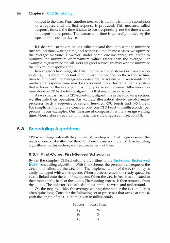
On the negative side, the average waiting time under the FCFS policy isoften quite long. Consider the following set of processes that arrive at time 0,with the length of the CPU burst given in milliseconds:

Process Burst Time

P1 24P2 3P3 3

6.3 Scheduling Algorithms 267

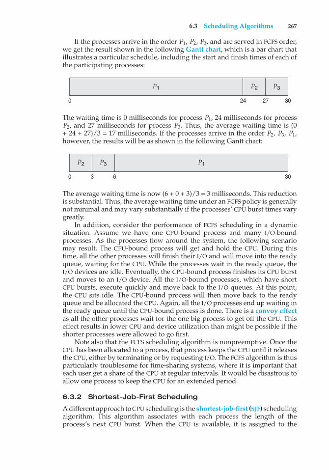
If the processes arrive in the order P1, P2, P3, and are served in FCFS order,we get the result shown in the following Gantt chart, which is a bar chart thatillustrates a particular schedule, including the start and finish times of each ofthe participating processes:

P1 P2 P3

3027240

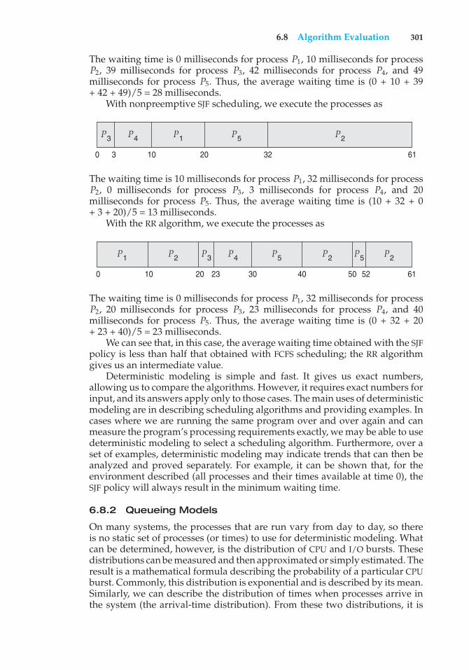
The waiting time is 0 milliseconds for process P1, 24 milliseconds for processP2, and 27 milliseconds for process P3. Thus, the average waiting time is (0+ 24 + 27)/3 = 17 milliseconds. If the processes arrive in the order P2, P3, P1,however, the results will be as shown in the following Gantt chart:

P1P2 P3

300 3 6

The average waiting time is now (6 + 0 + 3)/3 = 3 milliseconds. This reductionis substantial. Thus, the average waiting time under an FCFS policy is generallynot minimal and may vary substantially if the processes’ CPU burst times varygreatly.

In addition, consider the performance of FCFS scheduling in a dynamicsituation. Assume we have one CPU-bound process and many I/O-boundprocesses. As the processes flow around the system, the following scenariomay result. The CPU-bound process will get and hold the CPU. During thistime, all the other processes will finish their I/O and will move into the readyqueue, waiting for the CPU. While the processes wait in the ready queue, theI/O devices are idle. Eventually, the CPU-bound process finishes its CPU burstand moves to an I/O device. All the I/O-bound processes, which have shortCPU bursts, execute quickly and move back to the I/O queues. At this point,the CPU sits idle. The CPU-bound process will then move back to the readyqueue and be allocated the CPU. Again, all the I/O processes end up waiting inthe ready queue until the CPU-bound process is done. There is a convoy effectas all the other processes wait for the one big process to get off the CPU. Thiseffect results in lower CPU and device utilization than might be possible if theshorter processes were allowed to go first.

Note also that the FCFS scheduling algorithm is nonpreemptive. Once theCPU has been allocated to a process, that process keeps the CPU until it releasesthe CPU, either by terminating or by requesting I/O. The FCFS algorithm is thusparticularly troublesome for time-sharing systems, where it is important thateach user get a share of the CPU at regular intervals. It would be disastrous toallow one process to keep the CPU for an extended period.

6.3.2 Shortest-Job-First Scheduling

A different approach to CPU scheduling is the shortest-job-first (SJF) schedulingalgorithm. This algorithm associates with each process the length of theprocess’s next CPU burst. When the CPU is available, it is assigned to the


process that has the smallest next CPU burst. If the next CPU bursts of twoprocesses are the same, FCFS scheduling is used to break the tie. Note that amore appropriate term for this scheduling method would be the shortest-next-CPU-burst algorithm, because scheduling depends on the length of the nextCPU burst of a process, rather than its total length. We use the term SJF becausemost people and textbooks use this term to refer to this type of scheduling.

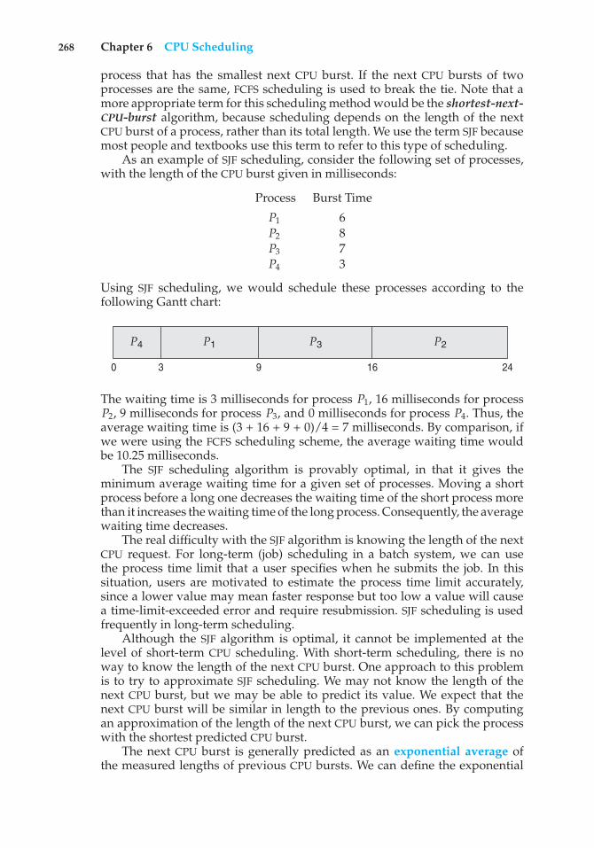
As an example of SJF scheduling, consider the following set of processes,with the length of the CPU burst given in milliseconds:

Process Burst Time

P1 6P2 8P3 7P4 3

Using SJF scheduling, we would schedule these processes according to thefollowing Gantt chart:

P3 P2P4 P1

241690 3

The waiting time is 3 milliseconds for process P1, 16 milliseconds for processP2, 9 milliseconds for process P3, and 0 milliseconds for process P4. Thus, theaverage waiting time is (3 + 16 + 9 + 0)/4 = 7 milliseconds. By comparison, ifwe were using the FCFS scheduling scheme, the average waiting time wouldbe 10.25 milliseconds.

The SJF scheduling algorithm is provably optimal, in that it gives theminimum average waiting time for a given set of processes. Moving a shortprocess before a long one decreases the waiting time of the short process morethan it increases the waiting time of the long process. Consequently, the averagewaiting time decreases.

The real difficulty with the SJF algorithm is knowing the length of the nextCPU request. For long-term (job) scheduling in a batch system, we can usethe process time limit that a user specifies when he submits the job. In thissituation, users are motivated to estimate the process time limit accurately,since a lower value may mean faster response but too low a value will causea time-limit-exceeded error and require resubmission. SJF scheduling is usedfrequently in long-term scheduling.

Although the SJF algorithm is optimal, it cannot be implemented at thelevel of short-term CPU scheduling. With short-term scheduling, there is noway to know the length of the next CPU burst. One approach to this problemis to try to approximate SJF scheduling. We may not know the length of thenext CPU burst, but we may be able to predict its value. We expect that thenext CPU burst will be similar in length to the previous ones. By computingan approximation of the length of the next CPU burst, we can pick the processwith the shortest predicted CPU burst.

The next CPU burst is generally predicted as an exponential average ofthe measured lengths of previous CPU bursts. We can define the exponential


6 4 6 4 13 13 13 …810 6 6 5 9 11 12 …

CPU burst (ti)

"guess" (τi)

ti

τi

2

time

4

6

8

10

12

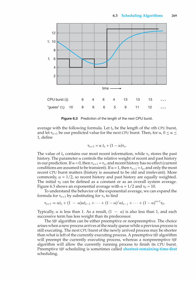
Figure 6.3 Prediction of the length of the next CPU burst.

average with the following formula. Let tn be the length of the nth CPU burst,and let �n+1 be our predicted value for the next CPU burst. Then, for �, 0 ≤ � ≤1, define

�n+1 = � tn + (1− �)�n.

The value of tn contains our most recent information, while �n stores the pasthistory. The parameter � controls the relative weight of recent and past historyin our prediction. If � = 0, then �n+1 = �n, and recent history has no effect (currentconditions are assumed to be transient). If � = 1, then �n+1 = tn, and only the mostrecent CPU burst matters (history is assumed to be old and irrelevant). Morecommonly, � = 1/2, so recent history and past history are equally weighted.The initial �0 can be defined as a constant or as an overall system average.Figure 6.3 shows an exponential average with � = 1/2 and �0 = 10.

To understand the behavior of the exponential average, we can expand theformula for �n+1 by substituting for �n to find

�n+1 = �tn + (1 − �)�tn−1 + · · · + (1− �) j �tn− j + · · · + (1− �)n+1�0.

Typically, � is less than 1. As a result, (1 − �) is also less than 1, and eachsuccessive term has less weight than its predecessor.

The SJF algorithm can be either preemptive or nonpreemptive. The choicearises when a new process arrives at the ready queue while a previous process isstill executing. The next CPU burst of the newly arrived process may be shorterthan what is left of the currently executing process. A preemptive SJF algorithmwill preempt the currently executing process, whereas a nonpreemptive SJFalgorithm will allow the currently running process to finish its CPU burst.Preemptive SJF scheduling is sometimes called shortest-remaining-time-firstscheduling.


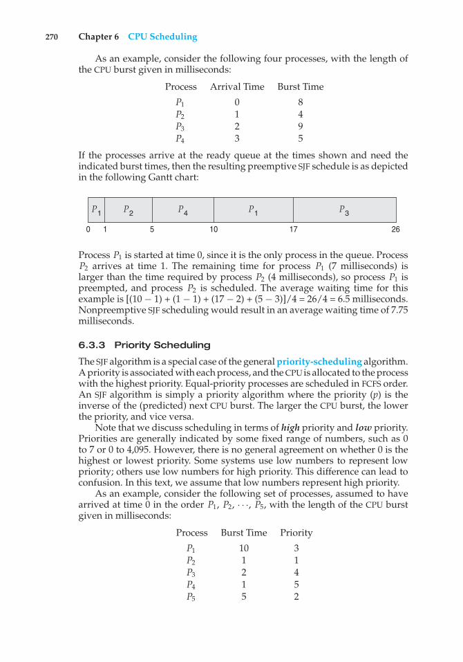
As an example, consider the following four processes, with the length ofthe CPU burst given in milliseconds:

Process Arrival Time Burst Time

P1 0 8P2 1 4P3 2 9P4 3 5

If the processes arrive at the ready queue at the times shown and need theindicated burst times, then the resulting preemptive SJF schedule is as depictedin the following Gantt chart:

P1 P3P1 P2 P4

2617100 1 5

Process P1 is started at time 0, since it is the only process in the queue. ProcessP2 arrives at time 1. The remaining time for process P1 (7 milliseconds) islarger than the time required by process P2 (4 milliseconds), so process P1 ispreempted, and process P2 is scheduled. The average waiting time for thisexample is [(10 − 1) + (1 − 1) + (17 − 2) + (5 − 3)]/4 = 26/4 = 6.5 milliseconds.Nonpreemptive SJF scheduling would result in an average waiting time of 7.75milliseconds.

6.3.3 Priority Scheduling

The SJF algorithm is a special case of the general priority-scheduling algorithm.A priority is associated with each process, and the CPU is allocated to the processwith the highest priority. Equal-priority processes are scheduled in FCFS order.An SJF algorithm is simply a priority algorithm where the priority (p) is theinverse of the (predicted) next CPU burst. The larger the CPU burst, the lowerthe priority, and vice versa.

Note that we discuss scheduling in terms of high priority and low priority.Priorities are generally indicated by some fixed range of numbers, such as 0to 7 or 0 to 4,095. However, there is no general agreement on whether 0 is thehighest or lowest priority. Some systems use low numbers to represent lowpriority; others use low numbers for high priority. This difference can lead toconfusion. In this text, we assume that low numbers represent high priority.

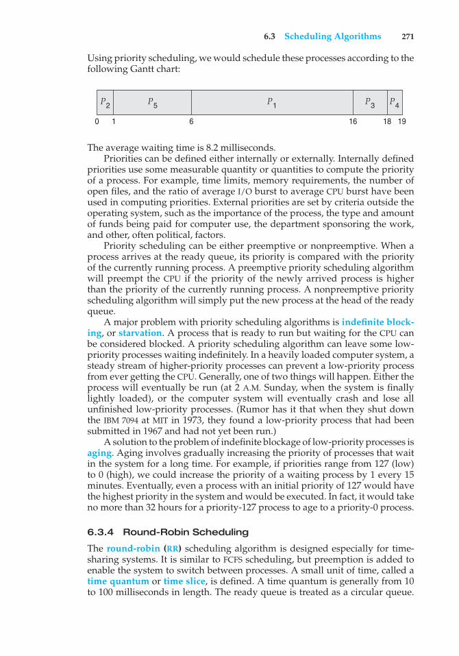
As an example, consider the following set of processes, assumed to havearrived at time 0 in the order P1, P2, · · ·, P5, with the length of the CPU burstgiven in milliseconds:

Process Burst Time Priority

P1 10 3P2 1 1P3 2 4P4 1 5P5 5 2


Using priority scheduling, we would schedule these processes according to thefollowing Gantt chart:

P1 P4P3P2 P5

19181660 1

The average waiting time is 8.2 milliseconds.Priorities can be defined either internally or externally. Internally defined

priorities use some measurable quantity or quantities to compute the priorityof a process. For example, time limits, memory requirements, the number ofopen files, and the ratio of average I/O burst to average CPU burst have beenused in computing priorities. External priorities are set by criteria outside theoperating system, such as the importance of the process, the type and amountof funds being paid for computer use, the department sponsoring the work,and other, often political, factors.

Priority scheduling can be either preemptive or nonpreemptive. When aprocess arrives at the ready queue, its priority is compared with the priorityof the currently running process. A preemptive priority scheduling algorithmwill preempt the CPU if the priority of the newly arrived process is higherthan the priority of the currently running process. A nonpreemptive priorityscheduling algorithm will simply put the new process at the head of the readyqueue.

A major problem with priority scheduling algorithms is indefinite block-ing, or starvation. A process that is ready to run but waiting for the CPU canbe considered blocked. A priority scheduling algorithm can leave some low-priority processes waiting indefinitely. In a heavily loaded computer system, asteady stream of higher-priority processes can prevent a low-priority processfrom ever getting the CPU. Generally, one of two things will happen. Either theprocess will eventually be run (at 2 A.M. Sunday, when the system is finallylightly loaded), or the computer system will eventually crash and lose allunfinished low-priority processes. (Rumor has it that when they shut downthe IBM 7094 at MIT in 1973, they found a low-priority process that had beensubmitted in 1967 and had not yet been run.)

A solution to the problem of indefinite blockage of low-priority processes isaging. Aging involves gradually increasing the priority of processes that waitin the system for a long time. For example, if priorities range from 127 (low)to 0 (high), we could increase the priority of a waiting process by 1 every 15minutes. Eventually, even a process with an initial priority of 127 would havethe highest priority in the system and would be executed. In fact, it would takeno more than 32 hours for a priority-127 process to age to a priority-0 process.

6.3.4 Round-Robin Scheduling

The round-robin (RR) scheduling algorithm is designed especially for time-sharing systems. It is similar to FCFS scheduling, but preemption is added toenable the system to switch between processes. A small unit of time, called atime quantum or time slice, is defined. A time quantum is generally from 10to 100 milliseconds in length. The ready queue is treated as a circular queue.


The CPU scheduler goes around the ready queue, allocating the CPU to eachprocess for a time interval of up to 1 time quantum.

To implement RR scheduling, we again treat the ready queue as a FIFOqueue of processes. New processes are added to the tail of the ready queue.The CPU scheduler picks the first process from the ready queue, sets a timer tointerrupt after 1 time quantum, and dispatches the process.

One of two things will then happen. The process may have a CPU burst ofless than 1 time quantum. In this case, the process itself will release the CPUvoluntarily. The scheduler will then proceed to the next process in the readyqueue. If the CPU burst of the currently running process is longer than 1 timequantum, the timer will go off and will cause an interrupt to the operatingsystem. A context switch will be executed, and the process will be put at thetail of the ready queue. The CPU scheduler will then select the next process inthe ready queue.

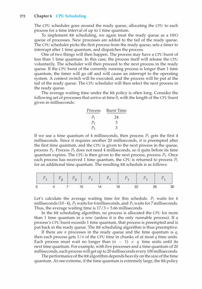
The average waiting time under the RR policy is often long. Consider thefollowing set of processes that arrive at time 0, with the length of the CPU burstgiven in milliseconds:

Process Burst Time

P1 24P2 3P3 3

If we use a time quantum of 4 milliseconds, then process P1 gets the first 4milliseconds. Since it requires another 20 milliseconds, it is preempted afterthe first time quantum, and the CPU is given to the next process in the queue,process P2. Process P2 does not need 4 milliseconds, so it quits before its timequantum expires. The CPU is then given to the next process, process P3. Onceeach process has received 1 time quantum, the CPU is returned to process P1for an additional time quantum. The resulting RR schedule is as follows:

P1P1 P1P1P1P1 P2

301814 26221070 4

P3

Let’s calculate the average waiting time for this schedule. P1 waits for 6milliseconds (10 - 4), P2 waits for 4 milliseconds, and P3 waits for 7 milliseconds.Thus, the average waiting time is 17/3 = 5.66 milliseconds.

In the RR scheduling algorithm, no process is allocated the CPU for morethan 1 time quantum in a row (unless it is the only runnable process). If aprocess’s CPU burst exceeds 1 time quantum, that process is preempted and isput back in the ready queue. The RR scheduling algorithm is thus preemptive.

If there are n processes in the ready queue and the time quantum is q,then each process gets 1/n of the CPU time in chunks of at most q time units.Each process must wait no longer than (n − 1) × q time units until itsnext time quantum. For example, with five processes and a time quantum of 20milliseconds, each process will get up to 20 milliseconds every 100 milliseconds.

The performance of the RR algorithm depends heavily on the size of the timequantum. At one extreme, if the time quantum is extremely large, the RR policy


process time � 10 quantum contextswitches

12 0

6 1

1 9

0 10

0 10

0 1 2 3 4 5 6 7 8 9 10

6

Figure 6.4 How a smaller time quantum increases context switches.

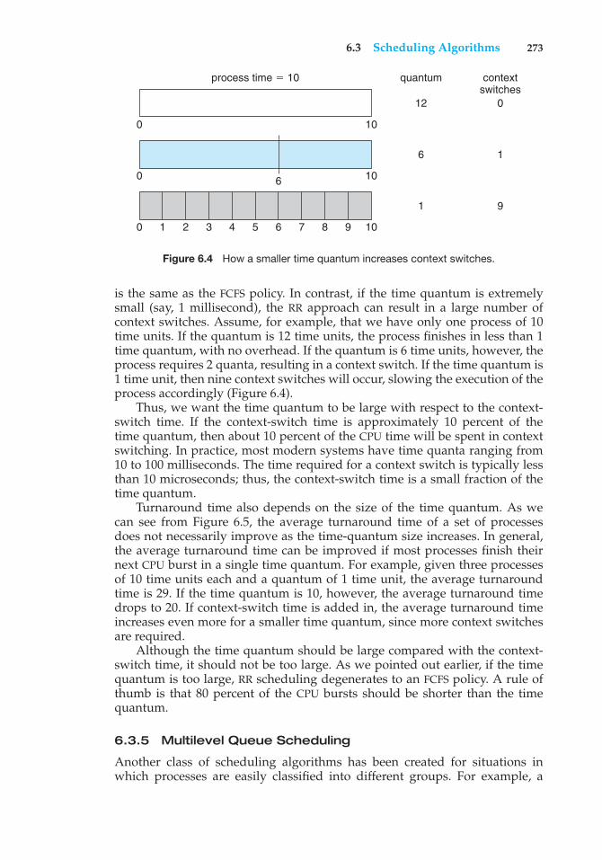
is the same as the FCFS policy. In contrast, if the time quantum is extremelysmall (say, 1 millisecond), the RR approach can result in a large number ofcontext switches. Assume, for example, that we have only one process of 10time units. If the quantum is 12 time units, the process finishes in less than 1time quantum, with no overhead. If the quantum is 6 time units, however, theprocess requires 2 quanta, resulting in a context switch. If the time quantum is1 time unit, then nine context switches will occur, slowing the execution of theprocess accordingly (Figure 6.4).

Thus, we want the time quantum to be large with respect to the context-switch time. If the context-switch time is approximately 10 percent of thetime quantum, then about 10 percent of the CPU time will be spent in contextswitching. In practice, most modern systems have time quanta ranging from10 to 100 milliseconds. The time required for a context switch is typically lessthan 10 microseconds; thus, the context-switch time is a small fraction of thetime quantum.

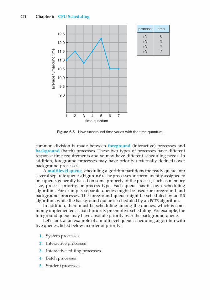
Turnaround time also depends on the size of the time quantum. As wecan see from Figure 6.5, the average turnaround time of a set of processesdoes not necessarily improve as the time-quantum size increases. In general,the average turnaround time can be improved if most processes finish theirnext CPU burst in a single time quantum. For example, given three processesof 10 time units each and a quantum of 1 time unit, the average turnaroundtime is 29. If the time quantum is 10, however, the average turnaround timedrops to 20. If context-switch time is added in, the average turnaround timeincreases even more for a smaller time quantum, since more context switchesare required.

Although the time quantum should be large compared with the context-switch time, it should not be too large. As we pointed out earlier, if the timequantum is too large, RR scheduling degenerates to an FCFS policy. A rule ofthumb is that 80 percent of the CPU bursts should be shorter than the timequantum.

6.3.5 Multilevel Queue Scheduling

Another class of scheduling algorithms has been created for situations inwhich processes are easily classified into different groups. For example, a


aver

age

turn

arou

nd ti

me

1

12.5

12.0

11.5

11.0

10.5

10.0

9.5

9.0

2 3 4time quantum

5 6 7

P1

P2

P3

P4

6 3 1 7

process time

Figure 6.5 How turnaround time varies with the time quantum.

common division is made between foreground (interactive) processes andbackground (batch) processes. These two types of processes have differentresponse-time requirements and so may have different scheduling needs. Inaddition, foreground processes may have priority (externally defined) overbackground processes.

A multilevel queue scheduling algorithm partitions the ready queue intoseveral separate queues (Figure 6.6). The processes are permanently assigned toone queue, generally based on some property of the process, such as memorysize, process priority, or process type. Each queue has its own schedulingalgorithm. For example, separate queues might be used for foreground andbackground processes. The foreground queue might be scheduled by an RRalgorithm, while the background queue is scheduled by an FCFS algorithm.

In addition, there must be scheduling among the queues, which is com-monly implemented as fixed-priority preemptive scheduling. For example, theforeground queue may have absolute priority over the background queue.

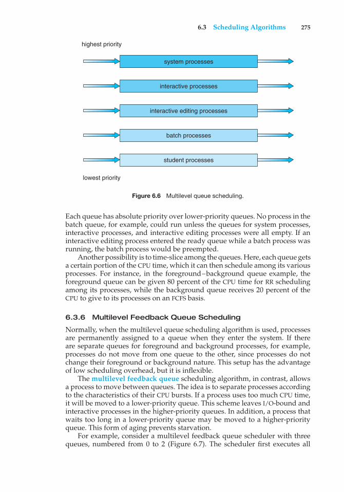
Let’s look at an example of a multilevel queue scheduling algorithm withfive queues, listed below in order of priority:

1. System processes

2. Interactive processes

3. Interactive editing processes

4. Batch processes

5. Student processes


system processes

highest priority

lowest priority

interactive processes

interactive editing processes

batch processes

student processes

Figure 6.6 Multilevel queue scheduling.

Each queue has absolute priority over lower-priority queues. No process in thebatch queue, for example, could run unless the queues for system processes,interactive processes, and interactive editing processes were all empty. If aninteractive editing process entered the ready queue while a batch process wasrunning, the batch process would be preempted.

Another possibility is to time-slice among the queues. Here, each queue getsa certain portion of the CPU time, which it can then schedule among its variousprocesses. For instance, in the foreground–background queue example, theforeground queue can be given 80 percent of the CPU time for RR schedulingamong its processes, while the background queue receives 20 percent of theCPU to give to its processes on an FCFS basis.

6.3.6 Multilevel Feedback Queue Scheduling

Normally, when the multilevel queue scheduling algorithm is used, processesare permanently assigned to a queue when they enter the system. If thereare separate queues for foreground and background processes, for example,processes do not move from one queue to the other, since processes do notchange their foreground or background nature. This setup has the advantageof low scheduling overhead, but it is inflexible.

The multilevel feedback queue scheduling algorithm, in contrast, allowsa process to move between queues. The idea is to separate processes accordingto the characteristics of their CPU bursts. If a process uses too much CPU time,it will be moved to a lower-priority queue. This scheme leaves I/O-bound andinteractive processes in the higher-priority queues. In addition, a process thatwaits too long in a lower-priority queue may be moved to a higher-priorityqueue. This form of aging prevents starvation.

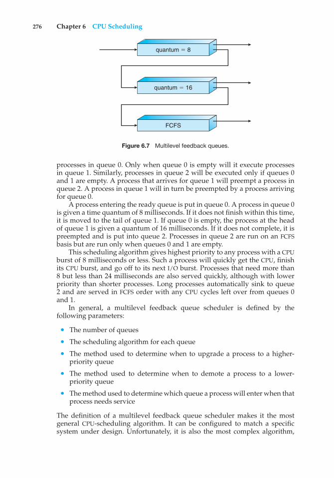
For example, consider a multilevel feedback queue scheduler with threequeues, numbered from 0 to 2 (Figure 6.7). The scheduler first executes all


quantum � 8

quantum � 16

FCFS

Figure 6.7 Multilevel feedback queues.

processes in queue 0. Only when queue 0 is empty will it execute processesin queue 1. Similarly, processes in queue 2 will be executed only if queues 0and 1 are empty. A process that arrives for queue 1 will preempt a process inqueue 2. A process in queue 1 will in turn be preempted by a process arrivingfor queue 0.

A process entering the ready queue is put in queue 0. A process in queue 0is given a time quantum of 8 milliseconds. If it does not finish within this time,it is moved to the tail of queue 1. If queue 0 is empty, the process at the headof queue 1 is given a quantum of 16 milliseconds. If it does not complete, it ispreempted and is put into queue 2. Processes in queue 2 are run on an FCFSbasis but are run only when queues 0 and 1 are empty.

This scheduling algorithm gives highest priority to any process with a CPUburst of 8 milliseconds or less. Such a process will quickly get the CPU, finishits CPU burst, and go off to its next I/O burst. Processes that need more than8 but less than 24 milliseconds are also served quickly, although with lowerpriority than shorter processes. Long processes automatically sink to queue2 and are served in FCFS order with any CPU cycles left over from queues 0and 1.

In general, a multilevel feedback queue scheduler is defined by thefollowing parameters:

• The number of queues

• The scheduling algorithm for each queue

• The method used to determine when to upgrade a process to a higher-priority queue

• The method used to determine when to demote a process to a lower-priority queue

• The method used to determine which queue a process will enter when thatprocess needs service

The definition of a multilevel feedback queue scheduler makes it the mostgeneral CPU-scheduling algorithm. It can be configured to match a specificsystem under design. Unfortunately, it is also the most complex algorithm,

6.4 Thread Scheduling 277

since defining the best scheduler requires some means by which to selectvalues for all the parameters.

6.4 Thread Scheduling

In Chapter 4, we introduced threads to the process model, distinguishingbetween user-level and kernel-level threads. On operating systems that supportthem, it is kernel-level threads—not processes—that are being scheduled bythe operating system. User-level threads are managed by a thread library,and the kernel is unaware of them. To run on a CPU, user-level threadsmust ultimately be mapped to an associated kernel-level thread, althoughthis mapping may be indirect and may use a lightweight process (LWP). In thissection, we explore scheduling issues involving user-level and kernel-levelthreads and offer specific examples of scheduling for Pthreads.

6.4.1 Contention Scope

One distinction between user-level and kernel-level threads lies in how theyare scheduled. On systems implementing the many-to-one (Section 4.3.1) andmany-to-many (Section 4.3.3) models, the thread library schedules user-levelthreads to run on an available LWP. This scheme is known as process-contention scope (PCS), since competition for the CPU takes place amongthreads belonging to the same process. (When we say the thread libraryschedules user threads onto available LWPs, we do not mean that the threadsare actually running on a CPU. That would require the operating system toschedule the kernel thread onto a physical CPU.) To decide which kernel-levelthread to schedule onto a CPU, the kernel uses system-contention scope (SCS).Competition for the CPU with SCS scheduling takes place among all threadsin the system. Systems using the one-to-one model (Section 4.3.2), such asWindows, Linux, and Solaris, schedule threads using only SCS.

Typically, PCS is done according to priority—the scheduler selects therunnable thread with the highest priority to run. User-level thread prioritiesare set by the programmer and are not adjusted by the thread library, althoughsome thread libraries may allow the programmer to change the priority ofa thread. It is important to note that PCS will typically preempt the threadcurrently running in favor of a higher-priority thread; however, there is noguarantee of time slicing (Section 6.3.4) among threads of equal priority.

6.4.2 Pthread Scheduling

We provided a sample POSIX Pthread program in Section 4.4.1, along with anintroduction to thread creation with Pthreads. Now, we highlight the POSIXPthread API that allows specifying PCS or SCS during thread creation. Pthreadsidentifies the following contention scope values:

• PTHREAD SCOPE PROCESS schedules threads using PCS scheduling.

• PTHREAD SCOPE SYSTEM schedules threads using SCS scheduling.


On systems implementing the many-to-many model, thePTHREAD SCOPE PROCESS policy schedules user-level threads onto availableLWPs. The number of LWPs is maintained by the thread library, perhaps usingscheduler activations (Section 4.6.5). The PTHREAD SCOPE SYSTEM schedulingpolicy will create and bind an LWP for each user-level thread on many-to-manysystems, effectively mapping threads using the one-to-one policy.

The Pthread IPC provides two functions for getting—and setting—thecontention scope policy:

• pthread attr setscope(pthread attr t *attr, int scope)

• pthread attr getscope(pthread attr t *attr, int *scope)

The first parameter for both functions contains a pointer to the attribute set forthe thread. The second parameter for the pthread attr setscope() functionis passed either the PTHREAD SCOPE SYSTEM or the PTHREAD SCOPE PROCESSvalue, indicating how the contention scope is to be set. In the case ofpthread attr getscope(), this second parameter contains a pointer to anint value that is set to the current value of the contention scope. If an erroroccurs, each of these functions returns a nonzero value.

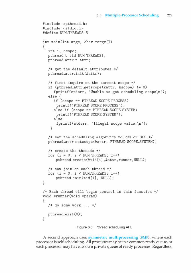
In Figure 6.8, we illustrate a Pthread scheduling API. The pro-gram first determines the existing contention scope and sets it toPTHREAD SCOPE SYSTEM. It then creates five separate threads that willrun using the SCS scheduling policy. Note that on some systems, only certaincontention scope values are allowed. For example, Linux and Mac OS Xsystems allow only PTHREAD SCOPE SYSTEM.

6.5 Multiple-Processor Scheduling

Our discussion thus far has focused on the problems of scheduling the CPU ina system with a single processor. If multiple CPUs are available, load sharingbecomes possible—but scheduling problems become correspondingly morecomplex. Many possibilities have been tried; and as we saw with single-processor CPU scheduling, there is no one best solution.

Here, we discuss several concerns in multiprocessor scheduling. Weconcentrate on systems in which the processors are identical—homogeneous—in terms of their functionality. We can then use any available processor torun any process in the queue. Note, however, that even with homogeneousmultiprocessors, there are sometimes limitations on scheduling. Consider asystem with an I/O device attached to a private bus of one processor. Processesthat wish to use that device must be scheduled to run on that processor.

6.5.1 Approaches to Multiple-Processor Scheduling

One approach to CPU scheduling in a multiprocessor system has all schedulingdecisions, I/O processing, and other system activities handled by a singleprocessor—the master server. The other processors execute only user code.This asymmetric multiprocessing is simple because only one processoraccesses the system data structures, reducing the need for data sharing.

6.5 Multiple-Processor Scheduling 279

#include <pthread.h>#include <stdio.h>#define NUM THREADS 5

int main(int argc, char *argv[]){

int i, scope;pthread t tid[NUM THREADS];pthread attr t attr;

/* get the default attributes */pthread attr init(&attr);

/* first inquire on the current scope */if (pthread attr getscope(&attr, &scope) != 0)

fprintf(stderr, "Unable to get scheduling scope\n");else {

if (scope == PTHREAD SCOPE PROCESS)printf("PTHREAD SCOPE PROCESS");

else if (scope == PTHREAD SCOPE SYSTEM)printf("PTHREAD SCOPE SYSTEM");

elsefprintf(stderr, "Illegal scope value.\n");

}

/* set the scheduling algorithm to PCS or SCS */pthread attr setscope(&attr, PTHREAD SCOPE SYSTEM);

/* create the threads */for (i = 0; i < NUM THREADS; i++)

pthread create(&tid[i],&attr,runner,NULL);

/* now join on each thread */for (i = 0; i < NUM THREADS; i++)

pthread join(tid[i], NULL);}

/* Each thread will begin control in this function */void *runner(void *param){

/* do some work ... */

pthread exit(0);}

Figure 6.8 Pthread scheduling API.

A second approach uses symmetric multiprocessing (SMP), where eachprocessor is self-scheduling. All processes may be in a common ready queue, oreach processor may have its own private queue of ready processes. Regardless,


scheduling proceeds by having the scheduler for each processor examine theready queue and select a process to execute. As we saw in Chapter 5, if we havemultiple processors trying to access and update a common data structure, thescheduler must be programmed carefully. We must ensure that two separateprocessors do not choose to schedule the same process and that processes arenot lost from the queue. Virtually all modern operating systems support SMP,including Windows, Linux, and Mac OS X. In the remainder of this section, wediscuss issues concerning SMP systems.

6.5.2 Processor Affinity

Consider what happens to cache memory when a process has been running ona specific processor. The data most recently accessed by the process populatethe cache for the processor. As a result, successive memory accesses by theprocess are often satisfied in cache memory. Now consider what happensif the process migrates to another processor. The contents of cache memorymust be invalidated for the first processor, and the cache for the secondprocessor must be repopulated. Because of the high cost of invalidating andrepopulating caches, most SMP systems try to avoid migration of processesfrom one processor to another and instead attempt to keep a process runningon the same processor. This is known as processor affinity—that is, a processhas an affinity for the processor on which it is currently running.

Processor affinity takes several forms. When an operating system has apolicy of attempting to keep a process running on the same processor—butnot guaranteeing that it will do so—we have a situation known as soft affinity.Here, the operating system will attempt to keep a process on a single processor,but it is possible for a process to migrate between processors. In contrast, somesystems provide system calls that support hard affinity, thereby allowing aprocess to specify a subset of processors on which it may run. Many systemsprovide both soft and hard affinity. For example, Linux implements soft affinity,but it also provides the sched setaffinity() system call, which supportshard affinity.

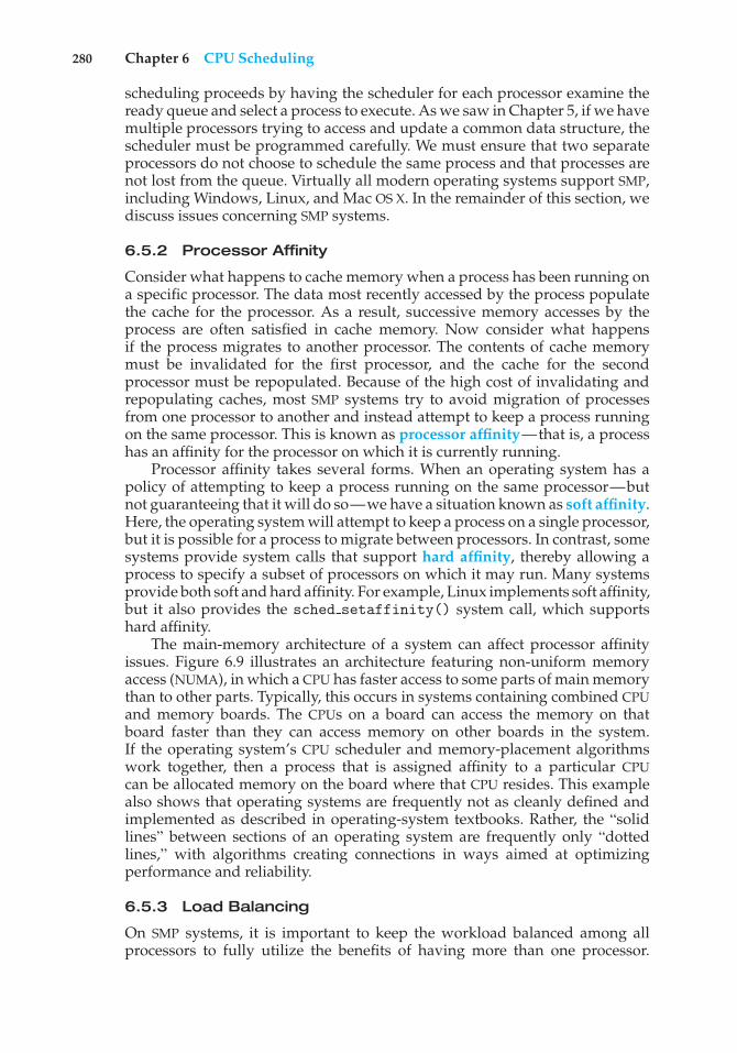
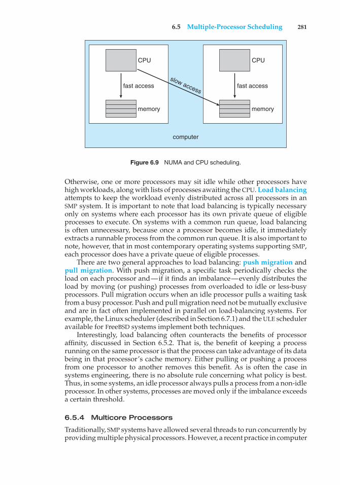
The main-memory architecture of a system can affect processor affinityissues. Figure 6.9 illustrates an architecture featuring non-uniform memoryaccess (NUMA), in which a CPU has faster access to some parts of main memorythan to other parts. Typically, this occurs in systems containing combined CPUand memory boards. The CPUs on a board can access the memory on thatboard faster than they can access memory on other boards in the system.If the operating system’s CPU scheduler and memory-placement algorithmswork together, then a process that is assigned affinity to a particular CPUcan be allocated memory on the board where that CPU resides. This examplealso shows that operating systems are frequently not as cleanly defined andimplemented as described in operating-system textbooks. Rather, the “solidlines” between sections of an operating system are frequently only “dottedlines,” with algorithms creating connections in ways aimed at optimizingperformance and reliability.

6.5.3 Load Balancing

On SMP systems, it is important to keep the workload balanced among allprocessors to fully utilize the benefits of having more than one processor.

6.5 Multiple-Processor Scheduling 281

CPU

fast access

memory

CPU

fast accessslow access

memory

computer

Figure 6.9 NUMA and CPU scheduling.

Otherwise, one or more processors may sit idle while other processors havehigh workloads, along with lists of processes awaiting the CPU. Load balancingattempts to keep the workload evenly distributed across all processors in anSMP system. It is important to note that load balancing is typically necessaryonly on systems where each processor has its own private queue of eligibleprocesses to execute. On systems with a common run queue, load balancingis often unnecessary, because once a processor becomes idle, it immediatelyextracts a runnable process from the common run queue. It is also important tonote, however, that in most contemporary operating systems supporting SMP,each processor does have a private queue of eligible processes.

There are two general approaches to load balancing: push migration andpull migration. With push migration, a specific task periodically checks theload on each processor and—if it finds an imbalance—evenly distributes theload by moving (or pushing) processes from overloaded to idle or less-busyprocessors. Pull migration occurs when an idle processor pulls a waiting taskfrom a busy processor. Push and pull migration need not be mutually exclusiveand are in fact often implemented in parallel on load-balancing systems. Forexample, the Linux scheduler (described in Section 6.7.1) and the ULE scheduleravailable for FreeBSD systems implement both techniques.

Interestingly, load balancing often counteracts the benefits of processoraffinity, discussed in Section 6.5.2. That is, the benefit of keeping a processrunning on the same processor is that the process can take advantage of its databeing in that processor’s cache memory. Either pulling or pushing a processfrom one processor to another removes this benefit. As is often the case insystems engineering, there is no absolute rule concerning what policy is best.Thus, in some systems, an idle processor always pulls a process from a non-idleprocessor. In other systems, processes are moved only if the imbalance exceedsa certain threshold.

6.5.4 Multicore Processors

Traditionally, SMP systems have allowed several threads to run concurrently byproviding multiple physical processors. However, a recent practice in computer


time

compute cycle memory stall cycle

threadC

C

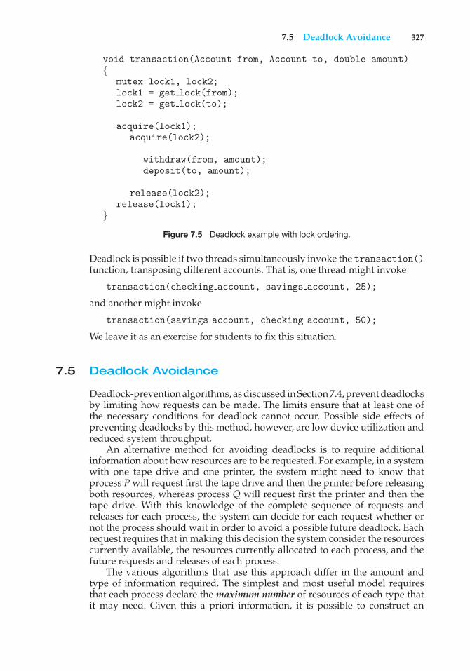
M C M C M

M

C M

Figure 6.10 Memory stall.

hardware has been to place multiple processor cores on the same physical chip,resulting in a multicore processor. Each core maintains its architectural stateand thus appears to the operating system to be a separate physical processor.SMP systems that use multicore processors are faster and consume less powerthan systems in which each processor has its own physical chip.

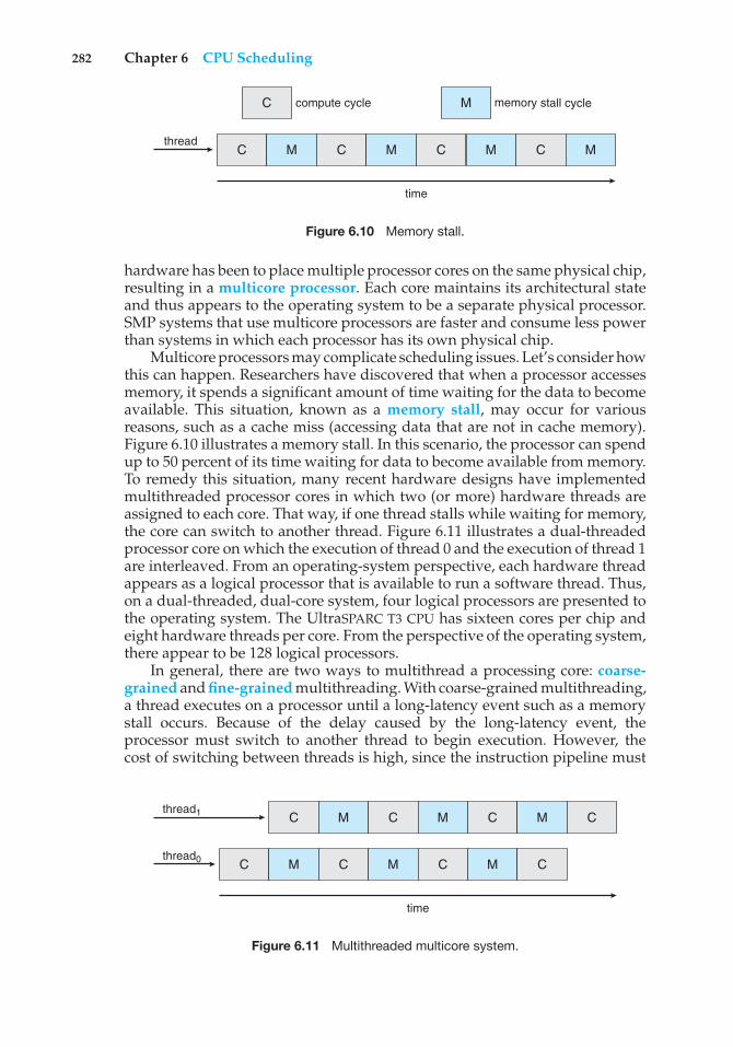
Multicore processors may complicate scheduling issues. Let’s consider howthis can happen. Researchers have discovered that when a processor accessesmemory, it spends a significant amount of time waiting for the data to becomeavailable. This situation, known as a memory stall, may occur for variousreasons, such as a cache miss (accessing data that are not in cache memory).Figure 6.10 illustrates a memory stall. In this scenario, the processor can spendup to 50 percent of its time waiting for data to become available from memory.To remedy this situation, many recent hardware designs have implementedmultithreaded processor cores in which two (or more) hardware threads areassigned to each core. That way, if one thread stalls while waiting for memory,the core can switch to another thread. Figure 6.11 illustrates a dual-threadedprocessor core on which the execution of thread 0 and the execution of thread 1are interleaved. From an operating-system perspective, each hardware threadappears as a logical processor that is available to run a software thread. Thus,on a dual-threaded, dual-core system, four logical processors are presented tothe operating system. The UltraSPARC T3 CPU has sixteen cores per chip andeight hardware threads per core. From the perspective of the operating system,there appear to be 128 logical processors.

In general, there are two ways to multithread a processing core: coarse-grained and fine-grained multithreading. With coarse-grained multithreading,a thread executes on a processor until a long-latency event such as a memorystall occurs. Because of the delay caused by the long-latency event, theprocessor must switch to another thread to begin execution. However, thecost of switching between threads is high, since the instruction pipeline must

time

thread0

thread1

C M C M C M C

C M C M C M C

Figure 6.11 Multithreaded multicore system.

6.6 Real-Time CPU Scheduling 283

be flushed before the other thread can begin execution on the processor core.Once this new thread begins execution, it begins filling the pipeline with itsinstructions. Fine-grained (or interleaved) multithreading switches betweenthreads at a much finer level of granularity—typically at the boundary of aninstruction cycle. However, the architectural design of fine-grained systemsincludes logic for thread switching. As a result, the cost of switching betweenthreads is small.

Notice that a multithreaded multicore processor actually requires twodifferent levels of scheduling. On one level are the scheduling decisions thatmust be made by the operating system as it chooses which software thread torun on each hardware thread (logical processor). For this level of scheduling,the operating system may choose any scheduling algorithm, such as thosedescribed in Section 6.3. A second level of scheduling specifies how each coredecides which hardware thread to run. There are several strategies to adoptin this situation. The UltraSPARC T3, mentioned earlier, uses a simple round-robin algorithm to schedule the eight hardware threads to each core. Anotherexample, the Intel Itanium, is a dual-core processor with two hardware-managed threads per core. Assigned to each hardware thread is a dynamicurgency value ranging from 0 to 7, with 0 representing the lowest urgencyand 7 the highest. The Itanium identifies five different events that may triggera thread switch. When one of these events occurs, the thread-switching logiccompares the urgency of the two threads and selects the thread with the highesturgency value to execute on the processor core.

6.6 Real-Time CPU Scheduling

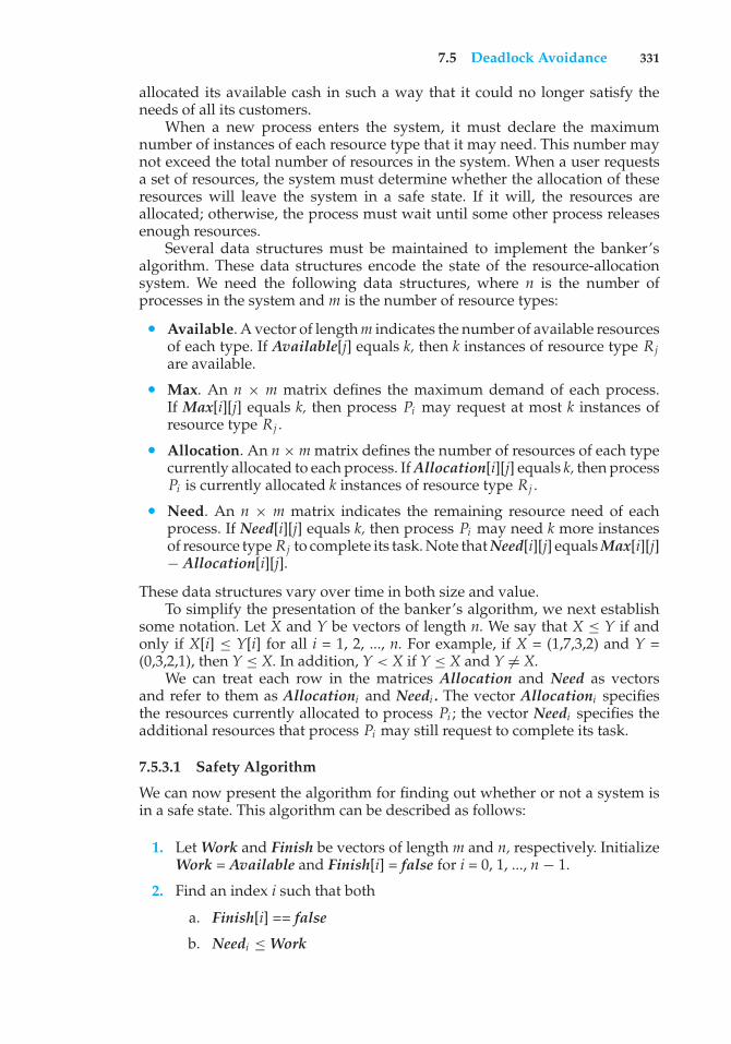
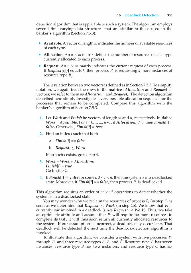
CPU scheduling for real-time operating systems involves special issues. Ingeneral, we can distinguish between soft real-time systems and hard real-timesystems. Soft real-time systems provide no guarantee as to when a criticalreal-time process will be scheduled. They guarantee only that the process willbe given preference over noncritical processes. Hard real-time systems havestricter requirements. A task must be serviced by its deadline; service after thedeadline has expired is the same as no service at all. In this section, we exploreseveral issues related to process scheduling in both soft and hard real-timeoperating systems.

6.6.1 Minimizing Latency

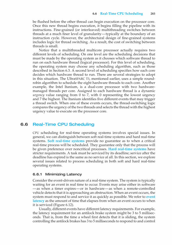
Consider the event-driven nature of a real-time system. The system is typicallywaiting for an event in real time to occur. Events may arise either in software—as when a timer expires—or in hardware—as when a remote-controlledvehicle detects that it is approaching an obstruction. When an event occurs, thesystem must respond to and service it as quickly as possible. We refer to eventlatency as the amount of time that elapses from when an event occurs to whenit is serviced (Figure 6.12).

Usually, different events have different latency requirements. For example,the latency requirement for an antilock brake system might be 3 to 5 millisec-onds. That is, from the time a wheel first detects that it is sliding, the systemcontrolling the antilock brakes has 3 to 5 milliseconds to respond to and control


t1t0

event latency

event E first occurs

real-time system responds to E

Time

Figure 6.12 Event latency.

the situation. Any response that takes longer might result in the automobile’sveering out of control. In contrast, an embedded system controlling radar inan airliner might tolerate a latency period of several seconds.

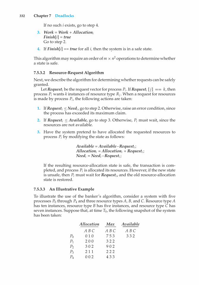
Two types of latencies affect the performance of real-time systems:

1. Interrupt latency

2. Dispatch latency

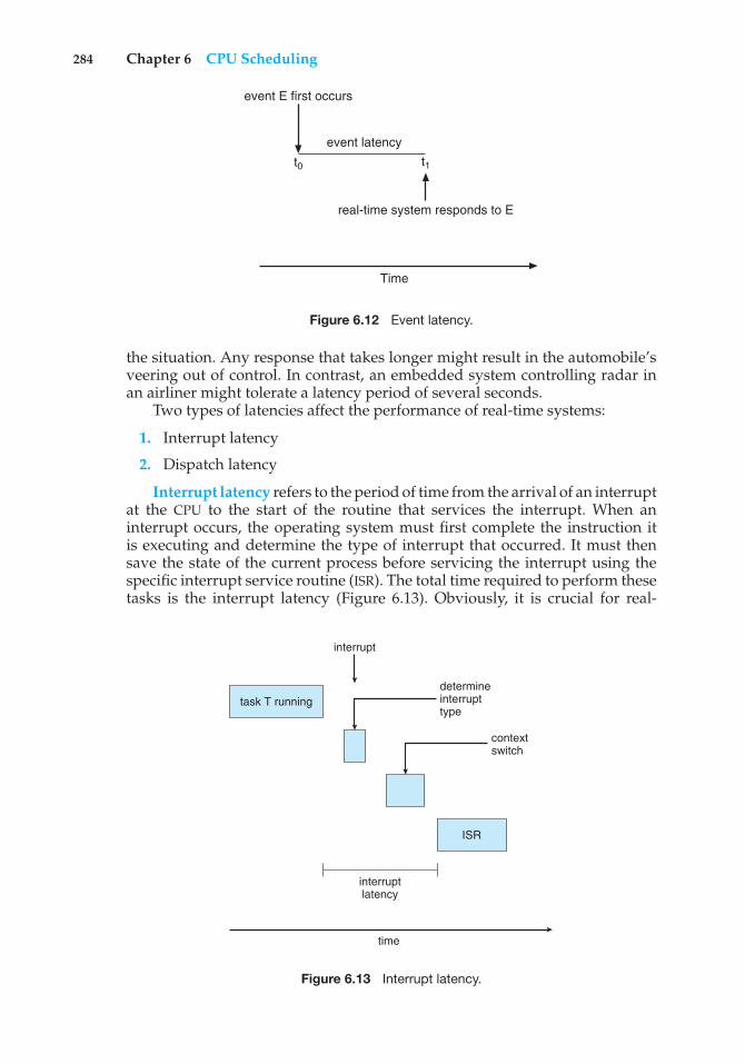
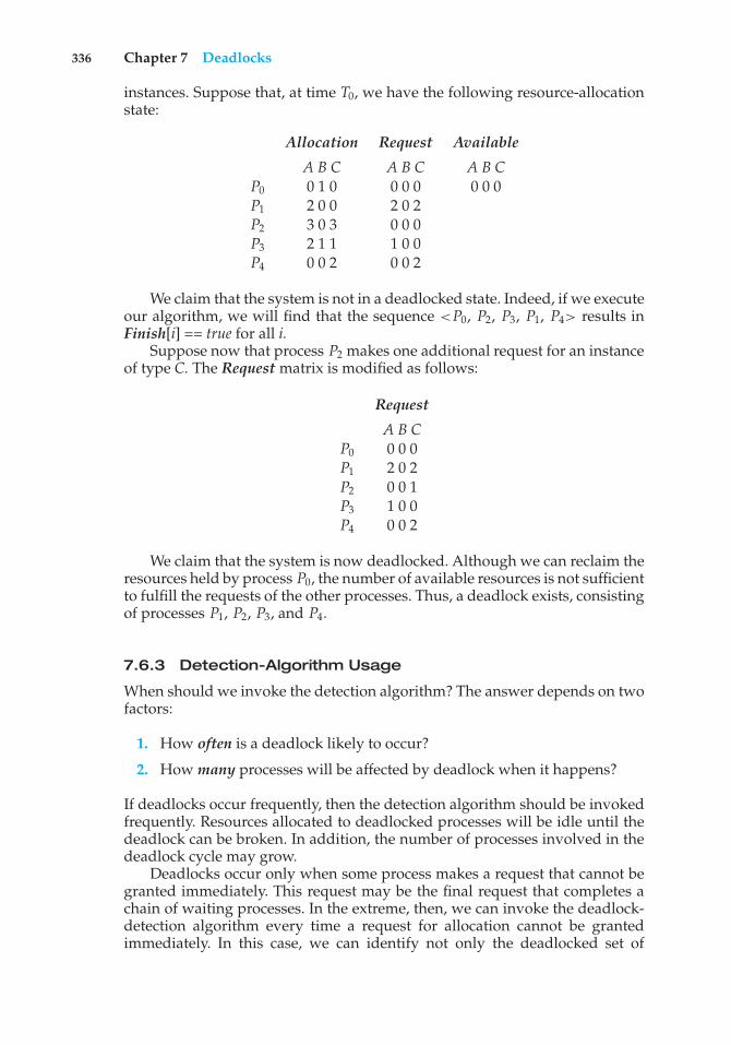
Interrupt latency refers to the period of time from the arrival of an interruptat the CPU to the start of the routine that services the interrupt. When aninterrupt occurs, the operating system must first complete the instruction itis executing and determine the type of interrupt that occurred. It must thensave the state of the current process before servicing the interrupt using thespecific interrupt service routine (ISR). The total time required to perform thesetasks is the interrupt latency (Figure 6.13). Obviously, it is crucial for real-

task T running

ISR

determineinterrupttype

interrupt

interruptlatency

contextswitch

time

Figure 6.13 Interrupt latency.


response to event

real-time process

execution

event

conflicts

time

dispatch

response interval

dispatch latency

process made availableinterrupt

processing

Figure 6.14 Dispatch latency.

time operating systems to minimize interrupt latency to ensure that real-timetasks receive immediate attention. Indeed, for hard real-time systems, interruptlatency must not simply be minimized, it must be bounded to meet the strictrequirements of these systems.

One important factor contributing to interrupt latency is the amount of timeinterrupts may be disabled while kernel data structures are being updated.Real-time operating systems require that interrupts be disabled for only veryshort periods of time.

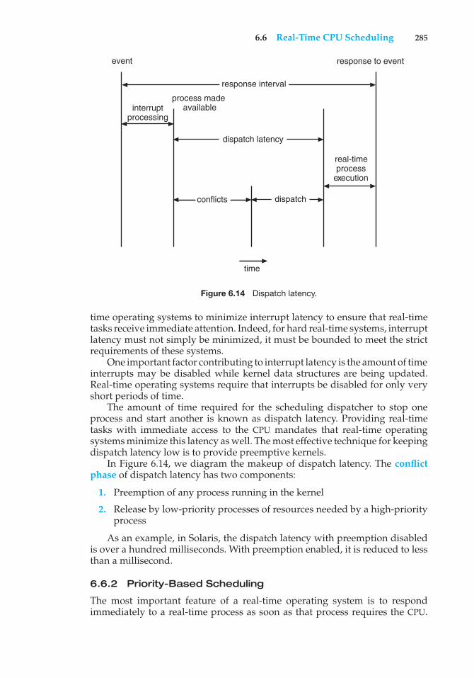
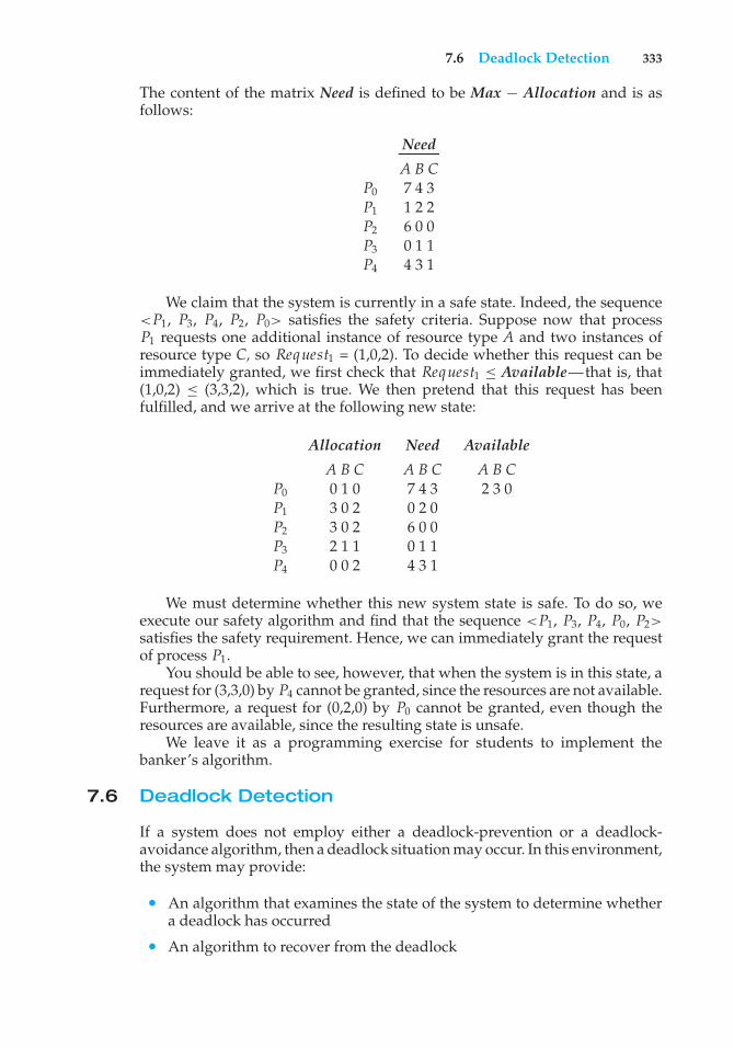
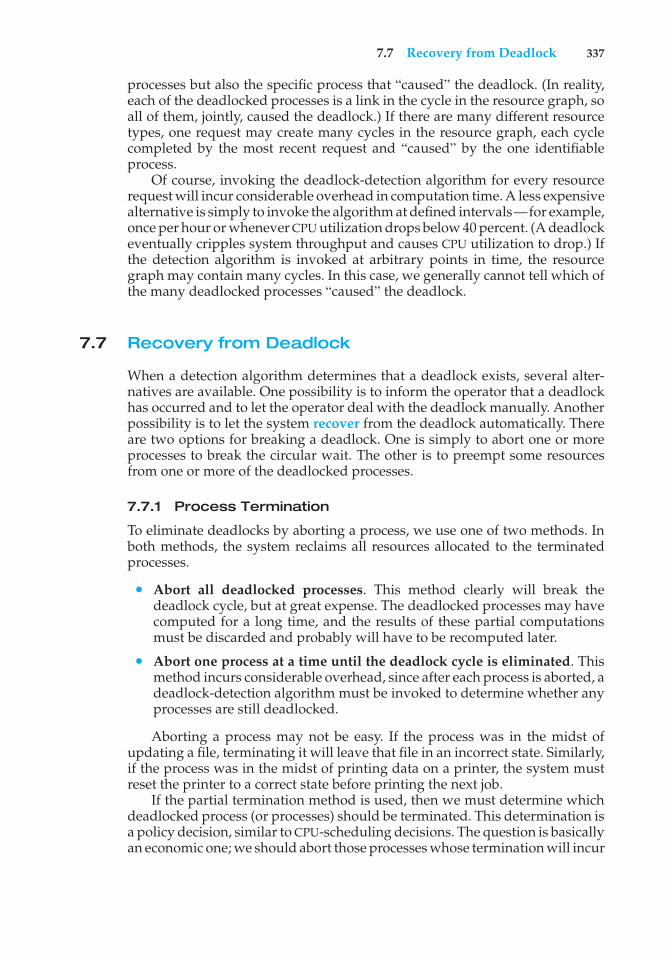
The amount of time required for the scheduling dispatcher to stop oneprocess and start another is known as dispatch latency. Providing real-timetasks with immediate access to the CPU mandates that real-time operatingsystems minimize this latency as well. The most effective technique for keepingdispatch latency low is to provide preemptive kernels.

In Figure 6.14, we diagram the makeup of dispatch latency. The conflictphase of dispatch latency has two components:

1. Preemption of any process running in the kernel

2. Release by low-priority processes of resources needed by a high-priorityprocess

As an example, in Solaris, the dispatch latency with preemption disabledis over a hundred milliseconds. With preemption enabled, it is reduced to lessthan a millisecond.

6.6.2 Priority-Based Scheduling

The most important feature of a real-time operating system is to respondimmediately to a real-time process as soon as that process requires the CPU.


As a result, the scheduler for a real-time operating system must support apriority-based algorithm with preemption. Recall that priority-based schedul-ing algorithms assign each process a priority based on its importance; moreimportant tasks are assigned higher priorities than those deemed less impor-tant. If the scheduler also supports preemption, a process currently runningon the CPU will be preempted if a higher-priority process becomes available torun.

Preemptive, priority-based scheduling algorithms are discussed in detail inSection 6.3.3, and Section 6.7 presents examples of the soft real-time schedulingfeatures of the Linux, Windows, and Solaris operating systems. Each ofthese systems assigns real-time processes the highest scheduling priority. Forexample, Windows has 32 different priority levels. The highest levels—priorityvalues 16 to 31—are reserved for real-time processes. Solaris and Linux havesimilar prioritization schemes.

Note that providing a preemptive, priority-based scheduler only guaran-tees soft real-time functionality. Hard real-time systems must further guaranteethat real-time tasks will be serviced in accord with their deadline requirements,and making such guarantees requires additional scheduling features. In theremainder of this section, we cover scheduling algorithms appropriate forhard real-time systems.

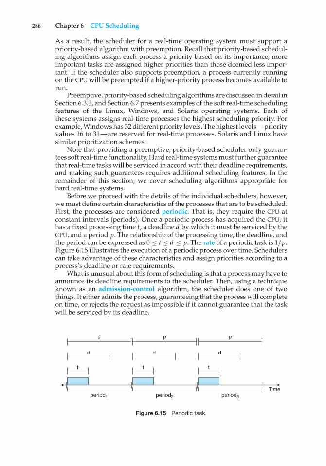
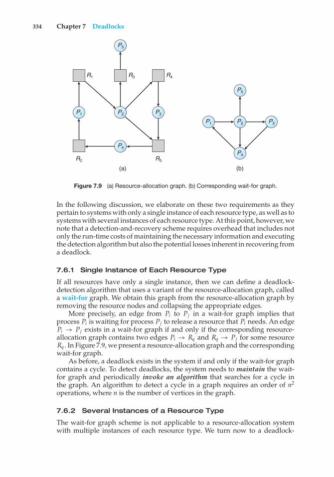
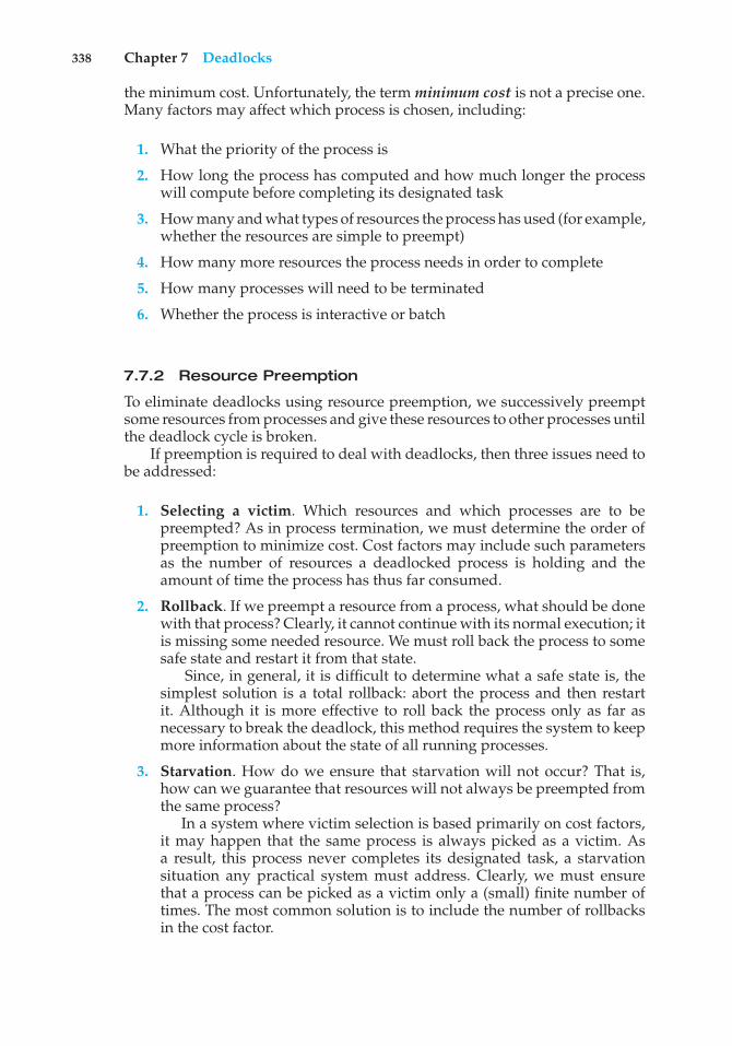
Before we proceed with the details of the individual schedulers, however,we must define certain characteristics of the processes that are to be scheduled.First, the processes are considered periodic. That is, they require the CPU atconstant intervals (periods). Once a periodic process has acquired the CPU, ithas a fixed processing time t, a deadline d by which it must be serviced by theCPU, and a period p. The relationship of the processing time, the deadline, andthe period can be expressed as 0 ≤ t ≤ d ≤ p. The rate of a periodic task is 1/p.Figure 6.15 illustrates the execution of a periodic process over time. Schedulerscan take advantage of these characteristics and assign priorities according to aprocess’s deadline or rate requirements.

What is unusual about this form of scheduling is that a process may have toannounce its deadline requirements to the scheduler. Then, using a techniqueknown as an admission-control algorithm, the scheduler does one of twothings. It either admits the process, guaranteeing that the process will completeon time, or rejects the request as impossible if it cannot guarantee that the taskwill be serviced by its deadline.

period1 period2 period3

Time

p p p

ddd

t tt

Figure 6.15 Periodic task.


0 10 20 30 40 50 60 70 80 12090 100 110

P1

P1

P1, P2

P2

deadlines

Figure 6.16 Scheduling of tasks when P2 has a higher priority than P1.

6.6.3 Rate-Monotonic Scheduling

The rate-monotonic scheduling algorithm schedules periodic tasks using astatic priority policy with preemption. If a lower-priority process is runningand a higher-priority process becomes available to run, it will preempt thelower-priority process. Upon entering the system, each periodic task is assigneda priority inversely based on its period. The shorter the period, the higher thepriority; the longer the period, the lower the priority. The rationale behind thispolicy is to assign a higher priority to tasks that require the CPU more often.Furthermore, rate-monotonic scheduling assumes that the processing time ofa periodic process is the same for each CPU burst. That is, every time a processacquires the CPU, the duration of its CPU burst is the same.

Let’s consider an example. We have two processes, P1 and P2. The periodsfor P1 and P2 are 50 and 100, respectively—that is, p1 = 50 and p2 = 100. Theprocessing times are t1 = 20 for P1 and t2 = 35 for P2. The deadline for eachprocess requires that it complete its CPU burst by the start of its next period.

We must first ask ourselves whether it is possible to schedule these tasksso that each meets its deadlines. If we measure the CPU utilization of a processPi as the ratio of its burst to its period—ti/pi —the CPU utilization of P1 is20/50 = 0.40 and that of P2 is 35/100 = 0.35, for a total CPU utilization of 75percent. Therefore, it seems we can schedule these tasks in such a way thatboth meet their deadlines and still leave the CPU with available cycles.

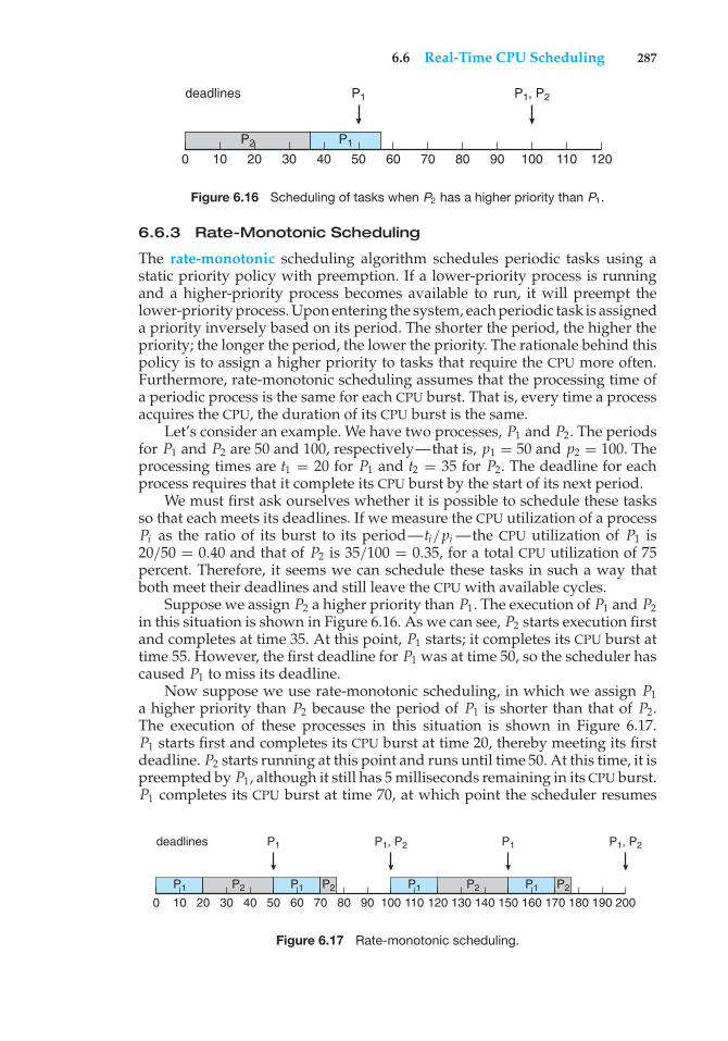
Suppose we assign P2 a higher priority than P1. The execution of P1 and P2in this situation is shown in Figure 6.16. As we can see, P2 starts execution firstand completes at time 35. At this point, P1 starts; it completes its CPU burst attime 55. However, the first deadline for P1 was at time 50, so the scheduler hascaused P1 to miss its deadline.

Now suppose we use rate-monotonic scheduling, in which we assign P1a higher priority than P2 because the period of P1 is shorter than that of P2.The execution of these processes in this situation is shown in Figure 6.17.P1 starts first and completes its CPU burst at time 20, thereby meeting its firstdeadline. P2 starts running at this point and runs until time 50. At this time, it ispreempted by P1, although it still has 5 milliseconds remaining in its CPU burst.P1 completes its CPU burst at time 70, at which point the scheduler resumes

0 10 20 30 40 50 60 70 80 120 130 140 150 160 170 180 190 20090 100 110

P1

P1

P1, P2

P1 P2

deadlines P1, P2P1

P2 P1 P2 P1 P2

Figure 6.17 Rate-monotonic scheduling.


P2. P2 completes its CPU burst at time 75, also meeting its first deadline. Thesystem is idle until time 100, when P1 is scheduled again.

Rate-monotonic scheduling is considered optimal in that if a set ofprocesses cannot be scheduled by this algorithm, it cannot be scheduled byany other algorithm that assigns static priorities. Let’s next examine a set ofprocesses that cannot be scheduled using the rate-monotonic algorithm.

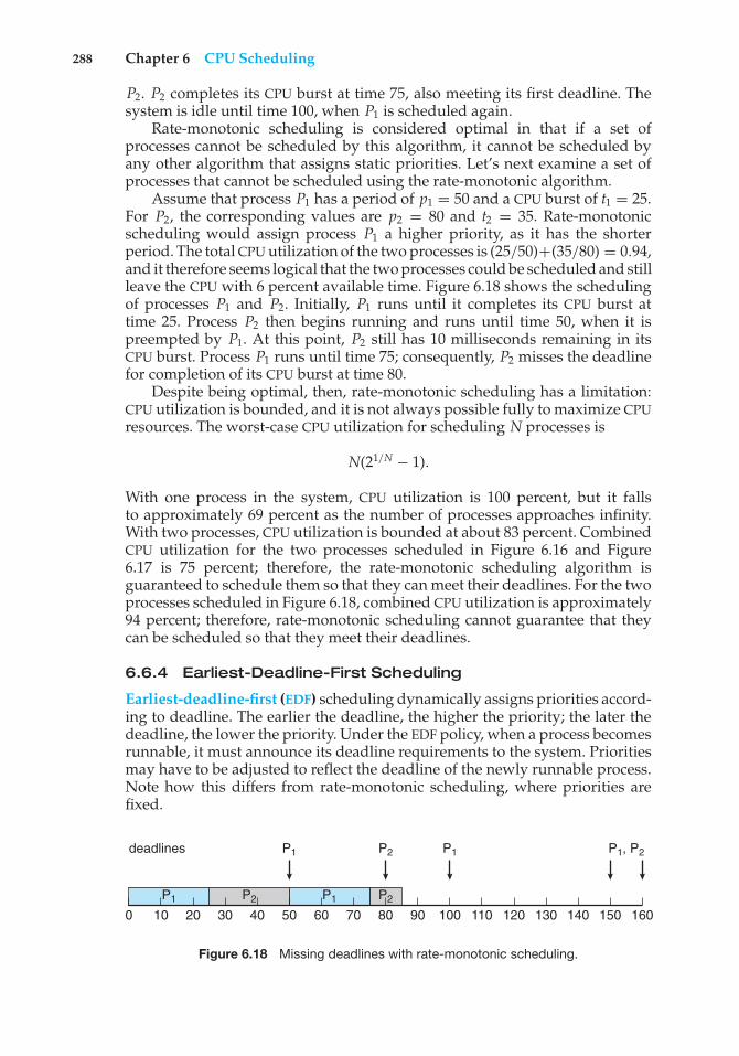
Assume that process P1 has a period of p1 = 50 and a CPU burst of t1 = 25.For P2, the corresponding values are p2 = 80 and t2 = 35. Rate-monotonicscheduling would assign process P1 a higher priority, as it has the shorterperiod. The total CPU utilization of the two processes is (25/50)+(35/80) = 0.94,and it therefore seems logical that the two processes could be scheduled and stillleave the CPU with 6 percent available time. Figure 6.18 shows the schedulingof processes P1 and P2. Initially, P1 runs until it completes its CPU burst attime 25. Process P2 then begins running and runs until time 50, when it ispreempted by P1. At this point, P2 still has 10 milliseconds remaining in itsCPU burst. Process P1 runs until time 75; consequently, P2 misses the deadlinefor completion of its CPU burst at time 80.

Despite being optimal, then, rate-monotonic scheduling has a limitation:CPU utilization is bounded, and it is not always possible fully to maximize CPUresources. The worst-case CPU utilization for scheduling N processes is

N(21/N − 1).

With one process in the system, CPU utilization is 100 percent, but it fallsto approximately 69 percent as the number of processes approaches infinity.With two processes, CPU utilization is bounded at about 83 percent. CombinedCPU utilization for the two processes scheduled in Figure 6.16 and Figure6.17 is 75 percent; therefore, the rate-monotonic scheduling algorithm isguaranteed to schedule them so that they can meet their deadlines. For the twoprocesses scheduled in Figure 6.18, combined CPU utilization is approximately94 percent; therefore, rate-monotonic scheduling cannot guarantee that theycan be scheduled so that they meet their deadlines.

6.6.4 Earliest-Deadline-First Scheduling

Earliest-deadline-first (EDF) scheduling dynamically assigns priorities accord-ing to deadline. The earlier the deadline, the higher the priority; the later thedeadline, the lower the priority. Under the EDF policy, when a process becomesrunnable, it must announce its deadline requirements to the system. Prioritiesmay have to be adjusted to reflect the deadline of the newly runnable process.Note how this differs from rate-monotonic scheduling, where priorities arefixed.

0 10 20 30 40 50 60 70 80 120 130 140 150 16090 100 110

P1

P1

P2

P1 P2

deadlines P1

P2

P1, P2

Figure 6.18 Missing deadlines with rate-monotonic scheduling.


0 10 20 30 40 50 60 70 80 120 130 140 150 16090 100 110

P1

P1 P1

P2

P1 P2

deadlines P2P1P1

P2 P2

Figure 6.19 Earliest-deadline-first scheduling.

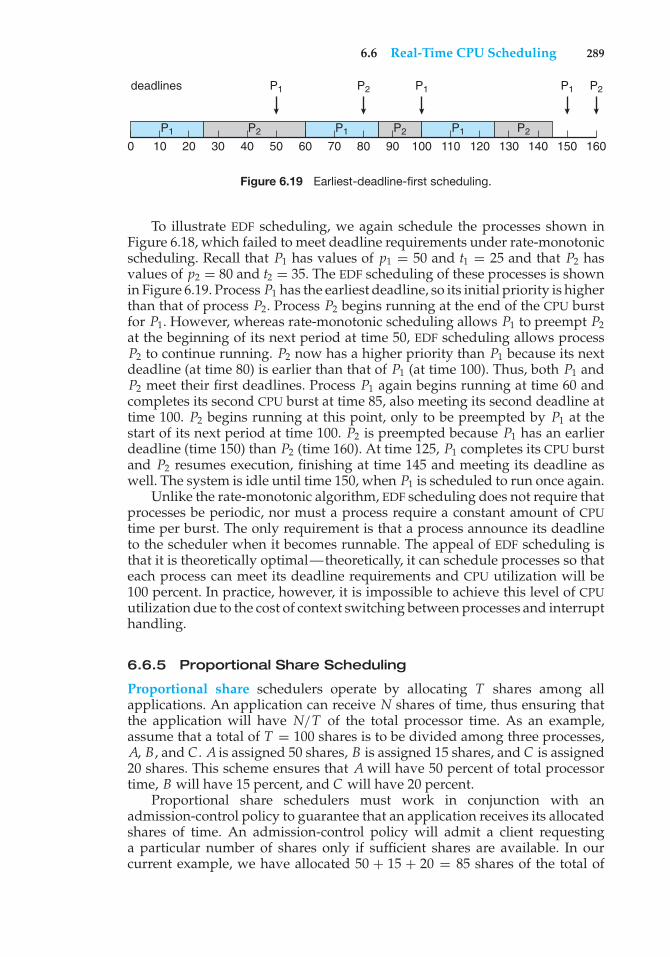
To illustrate EDF scheduling, we again schedule the processes shown inFigure 6.18, which failed to meet deadline requirements under rate-monotonicscheduling. Recall that P1 has values of p1 = 50 and t1 = 25 and that P2 hasvalues of p2 = 80 and t2 = 35. The EDF scheduling of these processes is shownin Figure 6.19. Process P1 has the earliest deadline, so its initial priority is higherthan that of process P2. Process P2 begins running at the end of the CPU burstfor P1. However, whereas rate-monotonic scheduling allows P1 to preempt P2at the beginning of its next period at time 50, EDF scheduling allows processP2 to continue running. P2 now has a higher priority than P1 because its nextdeadline (at time 80) is earlier than that of P1 (at time 100). Thus, both P1 andP2 meet their first deadlines. Process P1 again begins running at time 60 andcompletes its second CPU burst at time 85, also meeting its second deadline attime 100. P2 begins running at this point, only to be preempted by P1 at thestart of its next period at time 100. P2 is preempted because P1 has an earlierdeadline (time 150) than P2 (time 160). At time 125, P1 completes its CPU burstand P2 resumes execution, finishing at time 145 and meeting its deadline aswell. The system is idle until time 150, when P1 is scheduled to run once again.

Unlike the rate-monotonic algorithm, EDF scheduling does not require thatprocesses be periodic, nor must a process require a constant amount of CPUtime per burst. The only requirement is that a process announce its deadlineto the scheduler when it becomes runnable. The appeal of EDF scheduling isthat it is theoretically optimal—theoretically, it can schedule processes so thateach process can meet its deadline requirements and CPU utilization will be100 percent. In practice, however, it is impossible to achieve this level of CPUutilization due to the cost of context switching between processes and interrupthandling.

6.6.5 Proportional Share Scheduling

Proportional share schedulers operate by allocating T shares among allapplications. An application can receive N shares of time, thus ensuring thatthe application will have N/T of the total processor time. As an example,assume that a total of T = 100 shares is to be divided among three processes,A, B, and C . A is assigned 50 shares, B is assigned 15 shares, and C is assigned20 shares. This scheme ensures that A will have 50 percent of total processortime, B will have 15 percent, and C will have 20 percent.

Proportional share schedulers must work in conjunction with anadmission-control policy to guarantee that an application receives its allocatedshares of time. An admission-control policy will admit a client requestinga particular number of shares only if sufficient shares are available. In ourcurrent example, we have allocated 50 + 15 + 20 = 85 shares of the total of


100 shares. If a new process D requested 30 shares, the admission controllerwould deny D entry into the system.

6.6.6 POSIX Real-Time Scheduling

The POSIX standard also provides extensions for real-time computing—POSIX.1b. Here, we cover some of the POSIX API related to scheduling real-timethreads. POSIX defines two scheduling classes for real-time threads:

• SCHED FIFO

• SCHED RR

SCHED FIFO schedules threads according to a first-come, first-served policyusing a FIFO queue as outlined in Section 6.3.1. However, there is no time slicingamong threads of equal priority. Therefore, the highest-priority real-time threadat the front of the FIFO queue will be granted the CPU until it terminates orblocks. SCHED RR uses a round-robin policy. It is similar to SCHED FIFO exceptthat it provides time slicing among threads of equal priority. POSIX providesan additional scheduling class—SCHED OTHER—but its implementation isundefined and system specific; it may behave differently on different systems.

The POSIX API specifies the following two functions for getting and settingthe scheduling policy:

• pthread attr getsched policy(pthread attr t *attr, int*policy)

• pthread attr setsched policy(pthread attr t *attr, intpolicy)

The first parameter to both functions is a pointer to the set of attributes forthe thread. The second parameter is either (1) a pointer to an integer that isset to the current scheduling policy (for pthread attr getsched policy())or (2) an integer value (SCHED FIFO, SCHED RR, or SCHED OTHER) for thepthread attr setsched policy() function. Both functions return nonzerovalues if an error occurs.

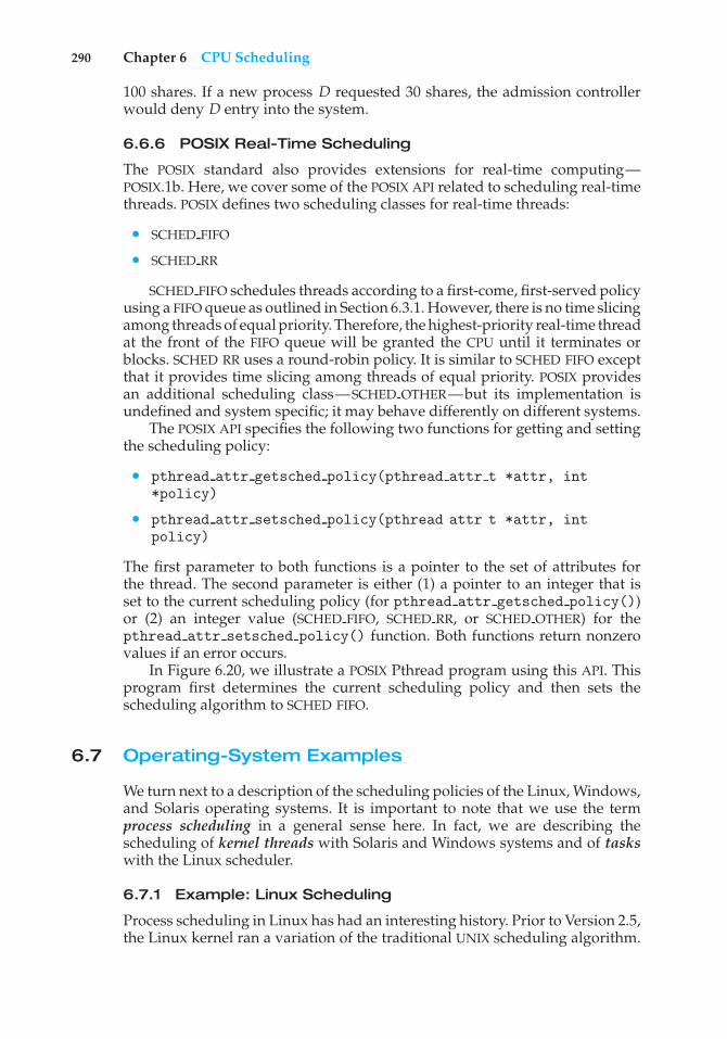
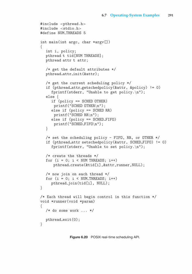
In Figure 6.20, we illustrate a POSIX Pthread program using this API. Thisprogram first determines the current scheduling policy and then sets thescheduling algorithm to SCHED FIFO.

6.7 Operating-System Examples

We turn next to a description of the scheduling policies of the Linux, Windows,and Solaris operating systems. It is important to note that we use the termprocess scheduling in a general sense here. In fact, we are describing thescheduling of kernel threads with Solaris and Windows systems and of taskswith the Linux scheduler.

6.7.1 Example: Linux Scheduling

Process scheduling in Linux has had an interesting history. Prior to Version 2.5,the Linux kernel ran a variation of the traditional UNIX scheduling algorithm.

6.7 Operating-System Examples 291

#include <pthread.h>#include <stdio.h>#define NUM THREADS 5

int main(int argc, char *argv[]){

int i, policy;pthread t tid[NUM THREADS];pthread attr t attr;

/* get the default attributes */pthread attr init(&attr);

/* get the current scheduling policy */if (pthread attr getschedpolicy(&attr, &policy) != 0)

fprintf(stderr, "Unable to get policy.\n");else {

if (policy == SCHED OTHER)printf("SCHED OTHER\n");

else if (policy == SCHED RR)printf("SCHED RR\n");

else if (policy == SCHED FIFO)printf("SCHED FIFO\n");

}

/* set the scheduling policy - FIFO, RR, or OTHER */if (pthread attr setschedpolicy(&attr, SCHED FIFO) != 0)

fprintf(stderr, "Unable to set policy.\n");

/* create the threads */for (i = 0; i < NUM THREADS; i++)

pthread create(&tid[i],&attr,runner,NULL);

/* now join on each thread */for (i = 0; i < NUM THREADS; i++)

pthread join(tid[i], NULL);}

/* Each thread will begin control in this function */void *runner(void *param){

/* do some work ... */

pthread exit(0);}

Figure 6.20 POSIX real-time scheduling API.


However, as this algorithm was not designed with SMP systems in mind, itdid not adequately support systems with multiple processors. In addition, itresulted in poor performance for systems with a large number of runnableprocesses. With Version 2.5 of the kernel, the scheduler was overhauled toinclude a scheduling algorithm—known as O(1)—that ran in constant timeregardless of the number of tasks in the system. The O(1) scheduler alsoprovided increased support for SMP systems, including processor affinity andload balancing between processors. However, in practice, although the O(1)scheduler delivered excellent performance on SMP systems, it led to poorresponse times for the interactive processes that are common on many desktopcomputer systems. During development of the 2.6 kernel, the scheduler wasagain revised; and in release 2.6.23 of the kernel, the Completely Fair Scheduler(CFS) became the default Linux scheduling algorithm.

Scheduling in the Linux system is based on scheduling classes. Each class isassigned a specific priority. By using different scheduling classes, the kernel canaccommodate different scheduling algorithms based on the needs of the systemand its processes. The scheduling criteria for a Linux server, for example, maybe different from those for a mobile device running Linux. To decide whichtask to run next, the scheduler selects the highest-priority task belonging tothe highest-priority scheduling class. Standard Linux kernels implement twoscheduling classes: (1) a default scheduling class using the CFS schedulingalgorithm and (2) a real-time scheduling class. We discuss each of these classeshere. New scheduling classes can, of course, be added.

Rather than using strict rules that associate a relative priority value withthe length of a time quantum, the CFS scheduler assigns a proportion of CPUprocessing time to each task. This proportion is calculated based on the nicevalue assigned to each task. Nice values range from −20 to +19, where anumerically lower nice value indicates a higher relative priority. Tasks withlower nice values receive a higher proportion of CPU processing time thantasks with higher nice values. The default nice value is 0. (The term nice comesfrom the idea that if a task increases its nice value from, say, 0 to+10, it is beingnice to other tasks in the system by lowering its relative priority.) CFS doesn’tuse discrete values of time slices and instead identifies a targeted latency,which is an interval of time during which every runnable task should run atleast once. Proportions of CPU time are allocated from the value of targetedlatency. In addition to having default and minimum values, targeted latencycan increase if the number of active tasks in the system grows beyond a certainthreshold.

The CFS scheduler doesn’t directly assign priorities. Rather, it records howlong each task has run by maintaining the virtual run time of each task usingthe per-task variable vruntime. The virtual run time is associated with a decayfactor based on the priority of a task: lower-priority tasks have higher ratesof decay than higher-priority tasks. For tasks at normal priority (nice valuesof 0), virtual run time is identical to actual physical run time. Thus, if a taskwith default priority runs for 200 milliseconds, its vruntime will also be 200milliseconds. However, if a lower-priority task runs for 200 milliseconds, itsvruntime will be higher than 200 milliseconds. Similarly, if a higher-prioritytask runs for 200 milliseconds, its vruntime will be less than 200 milliseconds.To decide which task to run next, the scheduler simply selects the task that hasthe smallest vruntime value. In addition, a higher-priority task that becomesavailable to run can preempt a lower-priority task.


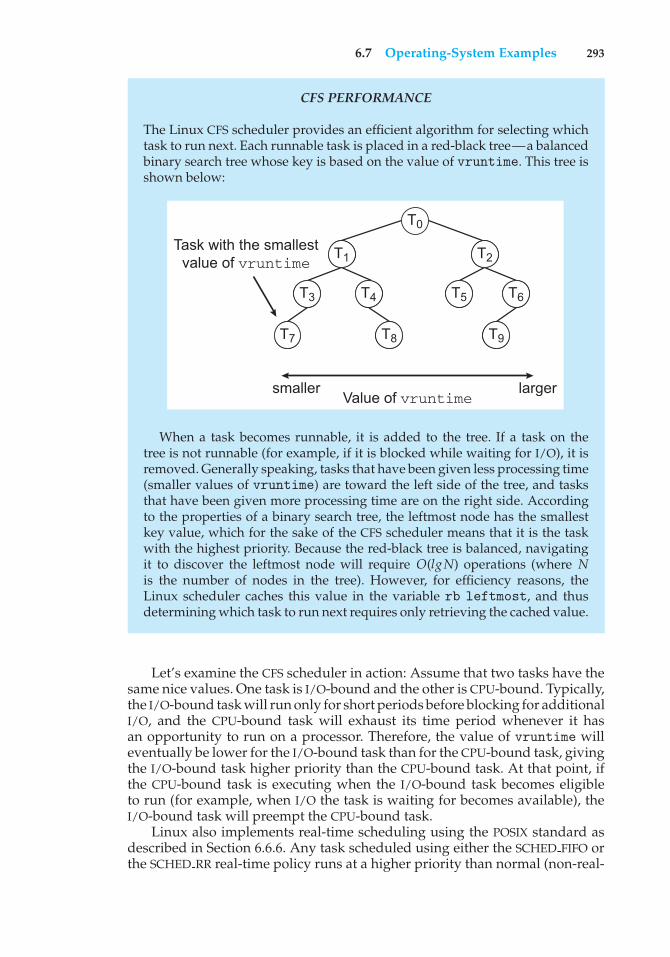
CFS PERFORMANCE

The Linux CFS scheduler provides an efficient algorithm for selecting whichtask to run next. Each runnable task is placed in a red-black tree—a balancedbinary search tree whose key is based on the value of vruntime. This tree isshown below:

T0

T2

T3 T5 T6

T1

T4

T9T7 T8

smaller larger

Task with the smallestvalue of vruntime

Value of vruntime

When a task becomes runnable, it is added to the tree. If a task on thetree is not runnable (for example, if it is blocked while waiting for I/O), it isremoved. Generally speaking, tasks that have been given less processing time(smaller values of vruntime) are toward the left side of the tree, and tasksthat have been given more processing time are on the right side. Accordingto the properties of a binary search tree, the leftmost node has the smallestkey value, which for the sake of the CFS scheduler means that it is the taskwith the highest priority. Because the red-black tree is balanced, navigatingit to discover the leftmost node will require O(lgN) operations (where Nis the number of nodes in the tree). However, for efficiency reasons, theLinux scheduler caches this value in the variable rb leftmost, and thusdetermining which task to run next requires only retrieving the cached value.

Let’s examine the CFS scheduler in action: Assume that two tasks have thesame nice values. One task is I/O-bound and the other is CPU-bound. Typically,the I/O-bound task will run only for short periods before blocking for additionalI/O, and the CPU-bound task will exhaust its time period whenever it hasan opportunity to run on a processor. Therefore, the value of vruntime willeventually be lower for the I/O-bound task than for the CPU-bound task, givingthe I/O-bound task higher priority than the CPU-bound task. At that point, ifthe CPU-bound task is executing when the I/O-bound task becomes eligibleto run (for example, when I/O the task is waiting for becomes available), theI/O-bound task will preempt the CPU-bound task.

Linux also implements real-time scheduling using the POSIX standard asdescribed in Section 6.6.6. Any task scheduled using either the SCHED FIFO orthe SCHED RR real-time policy runs at a higher priority than normal (non-real-


0 100 13999

Real-Time Normal

PriorityHigher Lower

Figure 6.21 Scheduling priorities on a Linux system.

time) tasks. Linux uses two separate priority ranges, one for real-time tasksand a second for normal tasks. Real-time tasks are assigned static prioritieswithin the range of 0 to 99, and normal (i.e. non real-time) tasks are assignedpriorities from 100 to 139. These two ranges map into a global priority schemewherein numerically lower values indicate higher relative priorities. Normaltasks are assigned a priority based on their nice values, where a value of –20maps to priority 100 and a nice value of +19 maps to 139. This scheme is shownin Figure 6.21.

6.7.2 Example: Windows Scheduling

Windows schedules threads using a priority-based, preemptive schedulingalgorithm. The Windows scheduler ensures that the highest-priority threadwill always run. The portion of the Windows kernel that handles schedulingis called the dispatcher. A thread selected to run by the dispatcher will rununtil it is preempted by a higher-priority thread, until it terminates, until itstime quantum ends, or until it calls a blocking system call, such as for I/O. If ahigher-priority real-time thread becomes ready while a lower-priority threadis running, the lower-priority thread will be preempted. This preemption givesa real-time thread preferential access to the CPU when the thread needs suchaccess.

The dispatcher uses a 32-level priority scheme to determine the order ofthread execution. Priorities are divided into two classes. The variable classcontains threads having priorities from 1 to 15, and the real-time class containsthreads with priorities ranging from 16 to 31. (There is also a thread running atpriority 0 that is used for memory management.) The dispatcher uses a queuefor each scheduling priority and traverses the set of queues from highest tolowest until it finds a thread that is ready to run. If no ready thread is found,the dispatcher will execute a special thread called the idle thread.

There is a relationship between the numeric priorities of the Windowskernel and the Windows API. The Windows API identifies the following sixpriority classes to which a process can belong:

• IDLE PRIORITY CLASS

• BELOW NORMAL PRIORITY CLASS

• NORMAL PRIORITY CLASS

• ABOVE NORMAL PRIORITY CLASS


• HIGH PRIORITY CLASS

• REALTIME PRIORITY CLASS

Processes are typically members of the NORMAL PRIORITY CLASS. A processbelongs to this class unless the parent of the process was a member of theIDLE PRIORITY CLASS or unless another class was specified when the processwas created. Additionally, the priority class of a process can be altered withthe SetPriorityClass() function in the Windows API. Priorities in all classesexcept the REALTIME PRIORITY CLASS are variable, meaning that the priority ofa thread belonging to one of these classes can change.

A thread within a given priority classes also has a relative priority. Thevalues for relative priorities include:

• IDLE

• LOWEST

• BELOW NORMAL

• NORMAL

• ABOVE NORMAL

• HIGHEST

• TIME CRITICAL

The priority of each thread is based on both the priority class it belongs toand its relative priority within that class. This relationship is shown in Figure6.22. The values of the priority classes appear in the top row. The left columncontains the values for the relative priorities. For example, if the relative priorityof a thread in the ABOVE NORMAL PRIORITY CLASS is NORMAL, the numericpriority of that thread is 10.

Furthermore, each thread has a base priority representing a value in thepriority range for the class to which the thread belongs. By default, the base

high abovenormal normal below

normalidlepriority

time-critical

real-time

31

26

25

24

23

22

16

15

15

14

13

12

11

1

15

12

11

10

9

8

1

15

10

9

8

7

6

1

15

8

7

6

5

4

1

15

6

5

4

3

2

1

highest

above normal

normal

lowest

idle

below normal

Figure 6.22 Windows thread priorities.


priority is the value of the NORMAL relative priority for that class. The basepriorities for each priority class are as follows:

• REALTIME PRIORITY CLASS—24

• HIGH PRIORITY CLASS—13

• ABOVE NORMAL PRIORITY CLASS—10

• NORMAL PRIORITY CLASS—8

• BELOW NORMAL PRIORITY CLASS—6

• IDLE PRIORITY CLASS—4

The initial priority of a thread is typically the base priority of the processthe thread belongs to, although the SetThreadPriority() function in theWindows API can also be used to modify a thread’s the base priority.

When a thread’s time quantum runs out, that thread is interrupted. If thethread is in the variable-priority class, its priority is lowered. The priority isnever lowered below the base priority, however. Lowering the priority tendsto limit the CPU consumption of compute-bound threads. When a variable-priority thread is released from a wait operation, the dispatcher boosts thepriority. The amount of the boost depends on what the thread was waiting for.For example, a thread waiting for keyboard I/O would get a large increase,whereas a thread waiting for a disk operation would get a moderate one.This strategy tends to give good response times to interactive threads thatare using the mouse and windows. It also enables I/O-bound threads to keepthe I/O devices busy while permitting compute-bound threads to use spareCPU cycles in the background. This strategy is used by several time-sharingoperating systems, including UNIX. In addition, the window with which theuser is currently interacting receives a priority boost to enhance its responsetime.

When a user is running an interactive program, the system needs to provideespecially good performance. For this reason, Windows has a special schedul-ing rule for processes in the NORMAL PRIORITY CLASS. Windows distinguishesbetween the foreground process that is currently selected on the screen andthe background processes that are not currently selected. When a processmoves into the foreground, Windows increases the scheduling quantum bysome factor—typically by 3. This increase gives the foreground process threetimes longer to run before a time-sharing preemption occurs.

Windows 7 introduced user-mode scheduling (UMS), which allows appli-cations to create and manage threads independently of the kernel. Thus,an application can create and schedule multiple threads without involvingthe Windows kernel scheduler. For applications that create a large numberof threads, scheduling threads in user mode is much more efficient thankernel-mode thread scheduling, as no kernel intervention is necessary.

Earlier versions of Windows provided a similar feature known as fibers,which allowed several user-mode threads (fibers) to be mapped to a singlekernel thread. However, fibers were of limited practical use. A fiber wasunable to make calls to the Windows API because all fibers had to share thethread environment block (TEB) of the thread on which they were running. This


presented a problem if a Windows API function placed state information intothe TEB for one fiber, only to have the information overwritten by a differentfiber. UMS overcomes this obstacle by providing each user-mode thread withits own thread context.

In addition, unlike fibers, UMS is not intended to be used directly bythe programmer. The details of writing user-mode schedulers can be verychallenging, and UMS does not include such a scheduler. Rather, the schedulerscome from programming language libraries that build on top of UMS. Forexample, Microsoft provides Concurrency Runtime (ConcRT), a concurrentprogramming framework for C++ that is designed for task-based parallelism(Section 4.2) on multicore processors. ConcRT provides a user-mode schedulertogether with facilities for decomposing programs into tasks, which can thenbe scheduled on the available processing cores. Further details on UMS can befound in Section 19.7.3.7.

6.7.3 Example: Solaris Scheduling

Solaris uses priority-based thread scheduling. Each thread belongs to one ofsix classes:

1. Time sharing (TS)

2. Interactive (IA)

3. Real time (RT)

4. System (SYS)

5. Fair share (FSS)

6. Fixed priority (FP)

Within each class there are different priorities and different scheduling algo-rithms.

The default scheduling class for a process is time sharing. The schedulingpolicy for the time-sharing class dynamically alters priorities and assigns timeslices of different lengths using a multilevel feedback queue. By default, thereis an inverse relationship between priorities and time slices. The higher thepriority, the smaller the time slice; and the lower the priority, the larger thetime slice. Interactive processes typically have a higher priority; CPU-boundprocesses, a lower priority. This scheduling policy gives good response timefor interactive processes and good throughput for CPU-bound processes. Theinteractive class uses the same scheduling policy as the time-sharing class, butit gives windowing applications—such as those created by the KDE or GNOMEwindow managers—a higher priority for better performance.

Figure 6.23 shows the dispatch table for scheduling time-sharing andinteractive threads. These two scheduling classes include 60 priority levels,but for brevity, we display only a handful. The dispatch table shown in Figure6.23 contains the following fields:

• Priority. The class-dependent priority for the time-sharing and interactiveclasses. A higher number indicates a higher priority.


timequantumpriority

returnfrom sleep

timequantumexpired

0

5

10

15

20

25

30

35

40

45

50

55

59

200

200

160

160

120

120

80

80

40

40

40

40

20

0

0

0

5

10

15

20

25

30

35

40

45

49

50

50

51

51

52

52

53

54

55

56

58

58

59

Figure 6.23 Solaris dispatch table for time-sharing and interactive threads.

• Time quantum. The time quantum for the associated priority. This illus-trates the inverse relationship between priorities and time quanta: thelowest priority (priority 0) has the highest time quantum (200 millisec-onds), and the highest priority (priority 59) has the lowest time quantum(20 milliseconds).

• Time quantum expired. The new priority of a thread that has usedits entire time quantum without blocking. Such threads are consideredCPU-intensive. As shown in the table, these threads have their prioritieslowered.

• Return from sleep. The priority of a thread that is returning from sleeping(such as from waiting for I/O). As the table illustrates, when I/O is availablefor a waiting thread, its priority is boosted to between 50 and 59, supportingthe scheduling policy of providing good response time for interactiveprocesses.

Threads in the real-time class are given the highest priority. A real-timeprocess will run before a process in any other class. This assignment allowsa real-time process to have a guaranteed response from the system withina bounded period of time. In general, however, few processes belong to thereal-time class.

Solaris uses the system class to run kernel threads, such as the schedulerand paging daemon. Once the priority of a system thread is established, it doesnot change. The system class is reserved for kernel use (user processes runningin kernel mode are not in the system class).


The fixed-priority and fair-share classes were introduced with Solaris 9.Threads in the fixed-priority class have the same priority range as those inthe time-sharing class; however, their priorities are not dynamically adjusted.The fair-share scheduling class uses CPU shares instead of priorities tomake scheduling decisions. CPU shares indicate entitlement to available CPUresources and are allocated to a set of processes (known as a project).

Each scheduling class includes a set of priorities. However, the schedulerconverts the class-specific priorities into global priorities and selects the threadwith the highest global priority to run. The selected thread runs on the CPUuntil it (1) blocks, (2) uses its time slice, or (3) is preempted by a higher-prioritythread. If there are multiple threads with the same priority, the scheduler usesa round-robin queue. Figure 6.24 illustrates how the six scheduling classesrelate to one another and how they map to global priorities. Notice that thekernel maintains ten threads for servicing interrupts. These threads do notbelong to any scheduling class and execute at the highest priority (160–169).As mentioned, Solaris has traditionally used the many-to-many model (Section4.3.3) but switched to the one-to-one model (Section 4.3.2) beginning withSolaris 9.

interrupt threads

169highest

lowest

first

schedulingorder

globalpriority

last

160159

100

6059

0

99

realtime (RT) threads

system (SYS) threads

fair share (FSS) threads

fixed priority (FX) threads

timeshare (TS) threads

interactive (IA) threads

Figure 6.24 Solaris scheduling.


6.8 Algorithm Evaluation

How do we select a CPU-scheduling algorithm for a particular system? As wesaw in Section 6.3, there are many scheduling algorithms, each with its ownparameters. As a result, selecting an algorithm can be difficult.

The first problem is defining the criteria to be used in selecting an algorithm.As we saw in Section 6.2, criteria are often defined in terms of CPU utilization,response time, or throughput. To select an algorithm, we must first definethe relative importance of these elements. Our criteria may include severalmeasures, such as these:

• Maximizing CPU utilization under the constraint that the maximumresponse time is 1 second

• Maximizing throughput such that turnaround time is (on average) linearlyproportional to total execution time

Once the selection criteria have been defined, we want to evaluate thealgorithms under consideration. We next describe the various evaluationmethods we can use.

6.8.1 Deterministic Modeling

One major class of evaluation methods is analytic evaluation. Analyticevaluation uses the given algorithm and the system workload to producea formula or number to evaluate the performance of the algorithm for thatworkload.

Deterministic modeling is one type of analytic evaluation. This methodtakes a particular predetermined workload and defines the performance of eachalgorithm for that workload. For example, assume that we have the workloadshown below. All five processes arrive at time 0, in the order given, with thelength of the CPU burst given in milliseconds:

Process Burst Time

P1 10P2 29P3 3P4 7P5 12

Consider the FCFS, SJF, and RR (quantum = 10 milliseconds) schedulingalgorithms for this set of processes. Which algorithm would give the minimumaverage waiting time?

For the FCFS algorithm, we would execute the processes as

P2 P5P3 P4P1

6139 49420 10

6.8 Algorithm Evaluation 301

The waiting time is 0 milliseconds for process P1, 10 milliseconds for processP2, 39 milliseconds for process P3, 42 milliseconds for process P4, and 49milliseconds for process P5. Thus, the average waiting time is (0 + 10 + 39+ 42 + 49)/5 = 28 milliseconds.

With nonpreemptive SJF scheduling, we execute the processes as

P5 P2P3 P4

613220100 3

P1


With the RR algorithm, we execute the processes as

P5 P5 P2P2 P2P3 P4

6130 40 50 5220 23100

P1


We can see that, in this case, the average waiting time obtained with the SJFpolicy is less than half that obtained with FCFS scheduling; the RR algorithmgives us an intermediate value.

Deterministic modeling is simple and fast. It gives us exact numbers,allowing us to compare the algorithms. However, it requires exact numbers forinput, and its answers apply only to those cases. The main uses of deterministicmodeling are in describing scheduling algorithms and providing examples. Incases where we are running the same program over and over again and canmeasure the program’s processing requirements exactly, we may be able to usedeterministic modeling to select a scheduling algorithm. Furthermore, over aset of examples, deterministic modeling may indicate trends that can then beanalyzed and proved separately. For example, it can be shown that, for theenvironment described (all processes and their times available at time 0), theSJF policy will always result in the minimum waiting time.

6.8.2 Queueing Models

On many systems, the processes that are run vary from day to day, so thereis no static set of processes (or times) to use for deterministic modeling. Whatcan be determined, however, is the distribution of CPU and I/O bursts. Thesedistributions can be measured and then approximated or simply estimated. Theresult is a mathematical formula describing the probability of a particular CPUburst. Commonly, this distribution is exponential and is described by its mean.Similarly, we can describe the distribution of times when processes arrive inthe system (the arrival-time distribution). From these two distributions, it is


possible to compute the average throughput, utilization, waiting time, and soon for most algorithms.

The computer system is described as a network of servers. Each server hasa queue of waiting processes. The CPU is a server with its ready queue, as isthe I/O system with its device queues. Knowing arrival rates and service rates,we can compute utilization, average queue length, average wait time, and soon. This area of study is called queueing-network analysis.

As an example, let n be the average queue length (excluding the processbeing serviced), let W be the average waiting time in the queue, and let � bethe average arrival rate for new processes in the queue (such as three processesper second). We expect that during the time W that a process waits, � × Wnew processes will arrive in the queue. If the system is in a steady state, thenthe number of processes leaving the queue must be equal to the number ofprocesses that arrive. Thus,

n = � ×W.

This equation, known as Little’s formula, is particularly useful because it isvalid for any scheduling algorithm and arrival distribution.

We can use Little’s formula to compute one of the three variables if weknow the other two. For example, if we know that 7 processes arrive everysecond (on average) and that there are normally 14 processes in the queue,then we can compute the average waiting time per process as 2 seconds.

Queueing analysis can be useful in comparing scheduling algorithms,but it also has limitations. At the moment, the classes of algorithms anddistributions that can be handled are fairly limited. The mathematics ofcomplicated algorithms and distributions can be difficult to work with. Thus,arrival and service distributions are often defined in mathematically tractable—but unrealistic—ways. It is also generally necessary to make a number ofindependent assumptions, which may not be accurate. As a result of thesedifficulties, queueing models are often only approximations of real systems,and the accuracy of the computed results may be questionable.

6.8.3 Simulations

To get a more accurate evaluation of scheduling algorithms, we can usesimulations. Running simulations involves programming a model of thecomputer system. Software data structures represent the major componentsof the system. The simulator has a variable representing a clock. As thisvariable’s value is increased, the simulator modifies the system state to reflectthe activities of the devices, the processes, and the scheduler. As the simulationexecutes, statistics that indicate algorithm performance are gathered andprinted.

The data to drive the simulation can be generated in several ways. Themost common method uses a random-number generator that is programmed togenerate processes, CPU burst times, arrivals, departures, and so on, accordingto probability distributions. The distributions can be defined mathematically(uniform, exponential, Poisson) or empirically. If a distribution is to be definedempirically, measurements of the actual system under study are taken. Theresults define the distribution of events in the real system; this distribution canthen be used to drive the simulation.

6.8 Algorithm Evaluation 303

actualprocess

execution

performancestatisticsfor FCFS

simulation

FCFS

performancestatisticsfor SJF

performancestatistics

for RR (q � 14)

trace tape

simulation

SJF

simulation

RR (q � 14)

• • •CPU 10I/O 213 CPU 12 I/O 112 CPU 2 I/O 147 CPU 173

• • •

Figure 6.25 Evaluation of CPU schedulers by simulation.

A distribution-driven simulation may be inaccurate, however, because ofrelationships between successive events in the real system. The frequencydistribution indicates only how many instances of each event occur; it does notindicate anything about the order of their occurrence. To correct this problem,we can use trace tapes. We create a trace tape by monitoring the real system andrecording the sequence of actual events (Figure 6.25). We then use this sequenceto drive the simulation. Trace tapes provide an excellent way to compare twoalgorithms on exactly the same set of real inputs. This method can produceaccurate results for its inputs.

Simulations can be expensive, often requiring hours of computer time. Amore detailed simulation provides more accurate results, but it also takes morecomputer time. In addition, trace tapes can require large amounts of storagespace. Finally, the design, coding, and debugging of the simulator can be amajor task.

6.8.4 Implementation

Even a simulation is of limited accuracy. The only completely accurate wayto evaluate a scheduling algorithm is to code it up, put it in the operatingsystem, and see how it works. This approach puts the actual algorithm in thereal system for evaluation under real operating conditions.

The major difficulty with this approach is the high cost. The expense isincurred not only in coding the algorithm and modifying the operating systemto support it (along with its required data structures) but also in the reactionof the users to a constantly changing operating system. Most users are notinterested in building a better operating system; they merely want to get theirprocesses executed and use their results. A constantly changing operatingsystem does not help the users to get their work done.

Another difficulty is that the environment in which the algorithm is usedwill change. The environment will change not only in the usual way, as new


programs are written and the types of problems change, but also as a resultof the performance of the scheduler. If short processes are given priority, thenusers may break larger processes into sets of smaller processes. If interactiveprocesses are given priority over noninteractive processes, then users mayswitch to interactive use.

For example, researchers designed one system that classified interactiveand noninteractive processes automatically by looking at the amount ofterminal I/O. If a process did not input or output to the terminal in a 1-secondinterval, the process was classified as noninteractive and was moved to alower-priority queue. In response to this policy, one programmer modified hisprograms to write an arbitrary character to the terminal at regular intervals ofless than 1 second. The system gave his programs a high priority, even thoughthe terminal output was completely meaningless.

The most flexible scheduling algorithms are those that can be alteredby the system managers or by the users so that they can be tuned fora specific application or set of applications. A workstation that performshigh-end graphical applications, for instance, may have scheduling needsdifferent from those of a Web server or file server. Some operating systems—particularly several versions of UNIX—allow the system manager to fine-tunethe scheduling parameters for a particular system configuration. For example,Solaris provides the dispadmin command to allow the system administratorto modify the parameters of the scheduling classes described in Section 6.7.3.

Another approach is to use APIs that can modify the priority of a processor thread. The Java, POSIX, and Windows API provide such functions. Thedownfall of this approach is that performance-tuning a system or applicationmost often does not result in improved performance in more general situations.

6.9 Summary

CPU scheduling is the task of selecting a waiting process from the ready queueand allocating the CPU to it. The CPU is allocated to the selected process by thedispatcher.

First-come, first-served (FCFS) scheduling is the simplest scheduling algo-rithm, but it can cause short processes to wait for very long processes. Shortest-job-first (SJF) scheduling is provably optimal, providing the shortest averagewaiting time. Implementing SJF scheduling is difficult, however, because pre-dicting the length of the next CPU burst is difficult. The SJF algorithm is a specialcase of the general priority scheduling algorithm, which simply allocates theCPU to the highest-priority process. Both priority and SJF scheduling may sufferfrom starvation. Aging is a technique to prevent starvation.

Round-robin (RR) scheduling is more appropriate for a time-shared (inter-active) system. RR scheduling allocates the CPU to the first process in the readyqueue for q time units, where q is the time quantum. After q time units, ifthe process has not relinquished the CPU, it is preempted, and the process isput at the tail of the ready queue. The major problem is the selection of thetime quantum. If the quantum is too large, RR scheduling degenerates to FCFSscheduling. If the quantum is too small, scheduling overhead in the form ofcontext-switch time becomes excessive.

Practice Exercises 305

The FCFS algorithm is nonpreemptive; the RR algorithm is preemptive. TheSJF and priority algorithms may be either preemptive or nonpreemptive.

Multilevel queue algorithms allow different algorithms to be used fordifferent classes of processes. The most common model includes a foregroundinteractive queue that uses RR scheduling and a background batch queue thatuses FCFS scheduling. Multilevel feedback queues allow processes to movefrom one queue to another.

Many contemporary computer systems support multiple processors andallow each processor to schedule itself independently. Typically, each processormaintains its own private queue of processes (or threads), all of which areavailable to run. Additional issues related to multiprocessor scheduling includeprocessor affinity, load balancing, and multicore processing.

A real-time computer system requires that results arrive within a deadlineperiod; results arriving after the deadline has passed are useless. Hard real-timesystems must guarantee that real-time tasks are serviced within their deadlineperiods. Soft real-time systems are less restrictive, assigning real-time taskshigher scheduling priority than other tasks.

Real-time scheduling algorithms include rate-monotonic and earliest-deadline-first scheduling. Rate-monotonic scheduling assigns tasks thatrequire the CPU more often a higher priority than tasks that require theCPU less often. Earliest-deadline-first scheduling assigns priority accordingto upcoming deadlines—the earlier the deadline, the higher the priority.Proportional share scheduling divides up processor time into shares andassigning each process a number of shares, thus guaranteeing each processa proportional share of CPU time. The POSIX Pthread API provides variousfeatures for scheduling real-time threads as well.

Operating systems supporting threads at the kernel level must schedulethreads—not processes—for execution. This is the case with Solaris andWindows. Both of these systems schedule threads using preemptive, priority-based scheduling algorithms, including support for real-time threads. TheLinux process scheduler uses a priority-based algorithm with real-time supportas well. The scheduling algorithms for these three operating systems typicallyfavor interactive over CPU-bound processes.

The wide variety of scheduling algorithms demands that we have methodsto select among algorithms. Analytic methods use mathematical analysis todetermine the performance of an algorithm. Simulation methods determineperformance by imitating the scheduling algorithm on a “representative”sample of processes and computing the resulting performance. However,simulation can at best provide an approximation of actual system performance.The only reliable technique for evaluating a scheduling algorithm is toimplement the algorithm on an actual system and monitor its performancein a “real-world” environment.

Practice Exercises

6.1 A CPU-scheduling algorithm determines an order for the executionof its scheduled processes. Given n processes to be scheduled on oneprocessor, how many different schedules are possible? Give a formulain terms of n.


6.2 Explain the difference between preemptive and nonpreemptive schedul-ing.

6.3 Suppose that the following processes arrive for execution at the timesindicated. Each process will run for the amount of time listed. Inanswering the questions, use nonpreemptive scheduling, and base alldecisions on the information you have at the time the decision must bemade.

Process Arrival Time Burst Time

P1 0.0 8P2 0.4 4P3 1.0 1

a. What is the average turnaround time for these processes with theFCFS scheduling algorithm?

b. What is the average turnaround time for these processes with theSJF scheduling algorithm?

c. The SJF algorithm is supposed to improve performance, but noticethat we chose to run process P1 at time 0 because we did not knowthat two shorter processes would arrive soon. Compute what theaverage turnaround time will be if the CPU is left idle for the first1 unit and then SJF scheduling is used. Remember that processesP1 and P2 are waiting during this idle time, so their waiting timemay increase. This algorithm could be called future-knowledgescheduling.

6.4 What advantage is there in having different time-quantum sizes atdifferent levels of a multilevel queueing system?

6.5 Many CPU-scheduling algorithms are parameterized. For example, theRR algorithm requires a parameter to indicate the time slice. Multilevelfeedback queues require parameters to define the number of queues, thescheduling algorithm for each queue, the criteria used to move processesbetween queues, and so on.

These algorithms are thus really sets of algorithms (for example, theset of RR algorithms for all time slices, and so on). One set of algorithmsmay include another (for example, the FCFS algorithm is the RR algorithmwith an infinite time quantum). What (if any) relation holds between thefollowing pairs of algorithm sets?

a. Priority and SJF

b. Multilevel feedback queues and FCFS

c. Priority and FCFS

d. RR and SJF

6.6 Suppose that a scheduling algorithm (at the level of short-term CPUscheduling) favors those processes that have used the least processor

Exercises 307

time in the recent past. Why will this algorithm favor I/O-boundprograms and yet not permanently starve CPU-bound programs?

6.7 Distinguish between PCS and SCS scheduling.

6.8 Assume that an operating system maps user-level threads to the kernelusing the many-to-many model and that the mapping is done throughthe use of LWPs. Furthermore, the system allows program developers tocreate real-time threads. Is it necessary to bind a real-time thread to anLWP?

6.9 The traditional UNIX scheduler enforces an inverse relationship betweenpriority numbers and priorities: the higher the number, the lower thepriority. The scheduler recalculates process priorities once per secondusing the following function:

Priority = (recent CPU usage / 2) + basewhere base = 60 and recent CPU usage refers to a value indicating howoften a process has used the CPU since priorities were last recalculated.

Assume that recent CPU usage is 40 for process P1, 18 for process P2,and 10 for process P3. What will be the new priorities for these threeprocesses when priorities are recalculated? Based on this information,does the traditional UNIX scheduler raise or lower the relative priorityof a CPU-bound process?

Exercises

6.10 Why is it important for the scheduler to distinguish I/O-bound programsfrom CPU-bound programs?

6.11 Discuss how the following pairs of scheduling criteria conflict in certainsettings.

a. CPU utilization and response time

b. Average turnaround time and maximum waiting time

c. I/O device utilization and CPU utilization

6.12 One technique for implementing lottery scheduling works by assigningprocesses lottery tickets, which are used for allocating CPU time. When-ever a scheduling decision has to be made, a lottery ticket is chosenat random, and the process holding that ticket gets the CPU. The BTVoperating system implements lottery scheduling by holding a lottery50 times each second, with each lottery winner getting 20 millisecondsof CPU time (20 milliseconds × 50 = 1 second). Describe how the BTVscheduler can ensure that higher-priority threads receive more attentionfrom the CPU than lower-priority threads.

6.13 In Chapter 5, we discussed possible race conditions on various kerneldata structures. Most scheduling algorithms maintain a run queue,which lists processes eligible to run on a processor. On multicore systems,there are two general options: (1) each processing core has its own run


queue, or (2) a single run queue is shared by all processing cores. Whatare the advantages and disadvantages of each of these approaches?

6.14 Consider the exponential average formula used to predict the length ofthe next CPU burst. What are the implications of assigning the followingvalues to the parameters used by the algorithm?

a. � = 0 and �0 = 100 milliseconds

b. � = 0.99 and �0 = 10 milliseconds

6.15 A variation of the round-robin scheduler is the regressive round-robinscheduler. This scheduler assigns each process a time quantum and apriority. The initial value of a time quantum is 50 milliseconds. However,every time a process has been allocated the CPU and uses its entire timequantum (does not block for I/O), 10 milliseconds is added to its timequantum, and its priority level is boosted. (The time quantum for aprocess can be increased to a maximum of 100 milliseconds.) When aprocess blocks before using its entire time quantum, its time quantum isreduced by 5 milliseconds, but its priority remains the same. What typeof process (CPU-bound or I/O-bound) does the regressive round-robinscheduler favor? Explain.

6.16 Consider the following set of processes, with the length of the CPU burstgiven in milliseconds:

Process Burst Time Priority

P1 2 2P2 1 1P3 8 4P4 4 2P5 5 3

The processes are assumed to have arrived in the order P1, P2, P3, P4, P5,all at time 0.

a. Draw four Gantt charts that illustrate the execution of theseprocesses using the following scheduling algorithms: FCFS, SJF,nonpreemptive priority (a larger priority number implies a higherpriority), and RR (quantum = 2).

b. What is the turnaround time of each process for each of thescheduling algorithms in part a?

c. What is the waiting time of each process for each of these schedul-ing algorithms?

d. Which of the algorithms results in the minimum average waitingtime (over all processes)?

6.17 The following processes are being scheduled using a preemptive, round-robin scheduling algorithm. Each process is assigned a numericalpriority, with a higher number indicating a higher relative priority.In addition to the processes listed below, the system also has an idle

Exercises 309

task (which consumes no CPU resources and is identified as Pidle ). Thistask has priority 0 and is scheduled whenever the system has no otheravailable processes to run. The length of a time quantum is 10 units.If a process is preempted by a higher-priority process, the preemptedprocess is placed at the end of the queue.

Thread Priority Burst ArrivalP1 40 20 0P2 30 25 25P3 30 25 30P4 35 15 60P5 5 10 100P6 10 10 105

a. Show the scheduling order of the processes using a Gantt chart.

b. What is the turnaround time for each process?

c. What is the waiting time for each process?

d. What is the CPU utilization rate?

6.18 The nice command is used to set the nice value of a process on Linux,as well as on other UNIX systems. Explain why some systems may allowany user to assign a process a nice value >= 0 yet allow only the rootuser to assign nice values < 0.

6.19 Which of the following scheduling algorithms could result in starvation?

a. First-come, first-served

b. Shortest job first

c. Round robin

d. Priority

6.20 Consider a variant of the RR scheduling algorithm in which the entriesin the ready queue are pointers to the PCBs.

a. What would be the effect of putting two pointers to the sameprocess in the ready queue?

b. What would be two major advantages and two disadvantages ofthis scheme?

c. How would you modify the basic RR algorithm to achieve the sameeffect without the duplicate pointers?

6.21 Consider a system running ten I/O-bound tasks and one CPU-boundtask. Assume that the I/O-bound tasks issue an I/O operation once forevery millisecond of CPU computing and that each I/O operation takes10 milliseconds to complete. Also assume that the context-switchingoverhead is 0.1 millisecond and that all processes are long-running tasks.Describe the CPU utilization for a round-robin scheduler when:


a. The time quantum is 1 millisecond

b. The time quantum is 10 milliseconds

6.22 Consider a system implementing multilevel queue scheduling. Whatstrategy can a computer user employ to maximize the amount of CPUtime allocated to the user’s process?

6.23 Consider a preemptive priority scheduling algorithm based on dynami-cally changing priorities. Larger priority numbers imply higher priority.When a process is waiting for the CPU (in the ready queue, but notrunning), its priority changes at a rate �. When it is running, its prioritychanges at a rate �. All processes are given a priority of 0 when theyenter the ready queue. The parameters � and � can be set to give manydifferent scheduling algorithms.

a. What is the algorithm that results from � > � > 0?

b. What is the algorithm that results from � < � < 0?

6.24 Explain the differences in how much the following scheduling algo-rithms discriminate in favor of short processes:

a. FCFS

b. RR

c. Multilevel feedback queues

6.25 Using the Windows scheduling algorithm, determine the numericpriority of each of the following threads.

a. A thread in the REALTIME PRIORITY CLASS with a relative priorityof NORMAL

b. A thread in the ABOVE NORMAL PRIORITY CLASS with a relativepriority of HIGHEST

c. A thread in the BELOW NORMAL PRIORITY CLASS with a relativepriority of ABOVE NORMAL

6.26 Assuming that no threads belong to the REALTIME PRIORITY CLASS andthat none may be assigned a TIME CRITICAL priority, what combinationof priority class and priority corresponds to the highest possible relativepriority in Windows scheduling?

6.27 Consider the scheduling algorithm in the Solaris operating system fortime-sharing threads.

a. What is the time quantum (in milliseconds) for a thread withpriority 15? With priority 40?

b. Assume that a thread with priority 50 has used its entire timequantum without blocking. What new priority will the schedulerassign this thread?

c. Assume that a thread with priority 20 blocks for I/O before its timequantum has expired. What new priority will the scheduler assignthis thread?

Bibliographical Notes 311

6.28 Assume that two tasks A and B are running on a Linux system. The nicevalues of Aand B are−5 and+5, respectively. Using the CFS scheduler asa guide, describe how the respective values of vruntime vary betweenthe two processes given each of the following scenarios:

• Both A and B are CPU-bound.

• A is I/O-bound, and B is CPU-bound.

• A is CPU-bound, and B is I/O-bound.

6.29 Discuss ways in which the priority inversion problem could beaddressed in a real-time system. Also discuss whether the solutionscould be implemented within the context of a proportional share sched-uler.

6.30 Under what circumstances is rate-monotonic scheduling inferior toearliest-deadline-first scheduling in meeting the deadlines associatedwith processes?

6.31 Consider two processes, P1 and P2, where p1 = 50, t1 = 25, p2 = 75, andt2 = 30.

a. Can these two processes be scheduled using rate-monotonicscheduling? Illustrate your answer using a Gantt chart such asthe ones in Figure 6.16–Figure 6.19.

b. Illustrate the scheduling of these two processes using earliest-deadline-first (EDF) scheduling.

6.32 Explain why interrupt and dispatch latency times must be bounded ina hard real-time system.

Bibliographical Notes

Feedback queues were originally implemented on the CTSS system described in[Corbato et al. (1962)]. This feedback queue scheduling system was analyzed by[Schrage (1967)]. The preemptive priority scheduling algorithm of Exercise 6.23was suggested by [Kleinrock (1975)]. The scheduling algorithms for hard real-time systems, such as rate monotonic scheduling and earliest-deadline-firstscheduling, are presented in [Liu and Layland (1973)].

[Anderson et al. (1989)], [Lewis and Berg (1998)], and [Philbin et al. (1996)]discuss thread scheduling. Multicore scheduling is examined in [McNairy andBhatia (2005)] and [Kongetira et al. (2005)].

[Fisher (1981)], [Hall et al. (1996)], and [Lowney et al. (1993)] describescheduling techniques that take into account information regarding processexecution times from previous runs.

Fair-share schedulers are covered by [Henry (1984)], [Woodside (1986)],and [Kay and Lauder (1988)].

Scheduling policies used in the UNIX V operating system are describedby [Bach (1987)]; those for UNIX FreeBSD 5.2 are presented by [McKusick andNeville-Neil (2005)]; and those for the Mach operating system are discussedby [Black (1990)]. [Love (2010)] and [Mauerer (2008)] cover scheduling in


Linux. [Faggioli et al. (2009)] discuss adding an EDF scheduler to the Linuxkernel. Details of the ULE scheduler can be found in [Roberson (2003)]. Solarisscheduling is described by [Mauro and McDougall (2007)]. [Russinovich andSolomon (2009)] discusses scheduling in Windows internals. [Butenhof (1997)]and [Lewis and Berg (1998)] describe scheduling in Pthreads systems. [Siddhaet al. (2007)] discuss scheduling challenges on multicore systems.

Bibliography

[Anderson et al. (1989)] T. E. Anderson, E. D. Lazowska, and H. M. Levy,“The Performance Implications of Thread Management Alternatives forShared-Memory Multiprocessors”, IEEE Transactions on Computers, Volume 38,Number 12 (1989), pages 1631–1644.

[Bach (1987)] M. J. Bach, The Design of the UNIX Operating System, Prentice Hall(1987).

[Black (1990)] D. L. Black, “Scheduling Support for Concurrency and Parallelismin the Mach Operating System”, IEEE Computer, Volume 23, Number 5 (1990),pages 35–43.

[Butenhof (1997)] D. Butenhof, Programming with POSIX Threads, Addison-Wesley (1997).

[Corbato et al. (1962)] F. J. Corbato, M. Merwin-Daggett, and R. C. Daley, “AnExperimental Time-Sharing System”, Proceedings of the AFIPS Fall Joint ComputerConference (1962), pages 335–344.

[Faggioli et al. (2009)] D. Faggioli, F. Checconi, M. Trimarchi, and C. Scordino,“An EDF scheduling class for the Linux kernel”, Proceedings of the 11th Real-TimeLinux Workshop (2009).

[Fisher (1981)] J. A. Fisher, “Trace Scheduling: A Technique for Global MicrocodeCompaction”, IEEE Transactions on Computers, Volume 30, Number 7 (1981),pages 478–490.

[Hall et al. (1996)] L. Hall, D. Shmoys, and J. Wein, “Scheduling To MinimizeAverage Completion Time: Off-line and On-line Algorithms”, SODA: ACM-SIAM Symposium on Discrete Algorithms (1996).

[Henry (1984)] G. Henry, “The Fair Share Scheduler”, AT&T Bell LaboratoriesTechnical Journal (1984).

[Kay and Lauder (1988)] J. Kay and P. Lauder, “A Fair Share Scheduler”, Com-munications of the ACM, Volume 31, Number 1 (1988), pages 44–55.

[Kleinrock (1975)] L. Kleinrock, Queueing Systems, Volume II: Computer Applica-tions, Wiley-Interscience (1975).

[Kongetira et al. (2005)] P. Kongetira, K. Aingaran, and K. Olukotun, “Niagara:A 32-Way Multithreaded SPARC Processor”, IEEE Micro Magazine, Volume 25,Number 2 (2005), pages 21–29.

Bibliography 313

[Lewis and Berg (1998)] B. Lewis and D. Berg, Multithreaded Programming withPthreads, Sun Microsystems Press (1998).

[Liu and Layland (1973)] C. L. Liu and J. W. Layland, “Scheduling Algorithmsfor Multiprogramming in a Hard Real-Time Environment”, Communications ofthe ACM, Volume 20, Number 1 (1973), pages 46–61.

[Love (2010)] R. Love, Linux Kernel Development, Third Edition, Developer’sLibrary (2010).

[Lowney et al. (1993)] P. G. Lowney, S. M. Freudenberger, T. J. Karzes, W. D.Lichtenstein, R. P. Nix, J. S. O’Donnell, and J. C. Ruttenberg, “The MultiflowTrace Scheduling Compiler”, Journal of Supercomputing, Volume 7, Number 1-2(1993), pages 51–142.

[Mauerer (2008)] W. Mauerer, Professional Linux Kernel Architecture, John Wileyand Sons (2008).

[Mauro and McDougall (2007)] J. Mauro and R. McDougall, Solaris Internals:Core Kernel Architecture, Prentice Hall (2007).

[McKusick and Neville-Neil (2005)] M. K. McKusick and G. V. Neville-Neil,The Design and Implementation of the FreeBSD UNIX Operating System, AddisonWesley (2005).

[McNairy and Bhatia (2005)] C. McNairy and R. Bhatia, “Montecito: A Dual–Core, Dual-Threaded Itanium Processor”, IEEE Micro Magazine, Volume 25,Number 2 (2005), pages 10–20.

[Philbin et al. (1996)] J. Philbin, J. Edler, O. J. Anshus, C. C. Douglas, and K. Li,“Thread Scheduling for Cache Locality”, Architectural Support for ProgrammingLanguages and Operating Systems (1996), pages 60–71.

[Roberson (2003)] J. Roberson, “ULE: A Modern Scheduler For FreeBSD”,Proceedings of the USENIX BSDCon Conference (2003), pages 17–28.

[Russinovich and Solomon (2009)] M. E. Russinovich and D. A. Solomon, Win-dows Internals: Including Windows Server 2008 and Windows Vista, Fifth Edition,Microsoft Press (2009).

[Schrage (1967)] L. E. Schrage, “The Queue M/G/I with Feedback to LowerPriority Queues”, Management Science, Volume 13, (1967), pages 466–474.

[Siddha et al. (2007)] S. Siddha, V. Pallipadi, and A. Mallick, “Process Schedul-ing Challenges in the Era of Multi-Core Processors”, Intel Technology Journal,Volume 11, Number 4 (2007).

[Woodside (1986)] C. Woodside, “Controllability of Computer PerformanceTradeoffs Obtained Using Controlled-Share Queue Schedulers”, IEEE Transac-tions on Software Engineering, Volume SE-12, Number 10 (1986), pages 1041–1048.

7C H A P T E R

Deadlocks

In a multiprogramming environment, several processes may compete for afinite number of resources. A process requests resources; if the resources arenot available at that time, the process enters a waiting state. Sometimes, awaiting process is never again able to change state, because the resources ithas requested are held by other waiting processes. This situation is calleda deadlock. We discussed this issue briefly in Chapter 5 in connection withsemaphores.

Perhaps the best illustration of a deadlock can be drawn from a law passedby the Kansas legislature early in the 20th century. It said, in part: “When twotrains approach each other at a crossing, both shall come to a full stop andneither shall start up again until the other has gone.”

In this chapter, we describe methods that an operating system can useto prevent or deal with deadlocks. Although some applications can identifyprograms that may deadlock, operating systems typically do not providedeadlock-prevention facilities, and it remains the responsibility of program-mers to ensure that they design deadlock-free programs. Deadlock problemscan only become more common, given current trends, including larger num-bers of processes, multithreaded programs, many more resources within asystem, and an emphasis on long-lived file and database servers rather thanbatch systems.

CHAPTER OBJECTIVES

• To develop a description of deadlocks, which prevent sets of concurrentprocesses from completing their tasks.

• To present a number of different methods for preventing or avoidingdeadlocks in a computer system.

7.1 System Model

A system consists of a finite number of resources to be distributed among anumber of competing processes. The resources may be partitioned into several

315

316 Chapter 7 Deadlocks

types (or classes), each consisting of some number of identical instances. CPUcycles, files, and I/O devices (such as printers and DVD drives) are examples ofresource types. If a system has two CPUs, then the resource type CPU has twoinstances. Similarly, the resource type printer may have five instances.

If a process requests an instance of a resource type, the allocation of anyinstance of the type should satisfy the request. If it does not, then the instancesare not identical, and the resource type classes have not been defined properly.For example, a system may have two printers. These two printers may bedefined to be in the same resource class if no one cares which printer printswhich output. However, if one printer is on the ninth floor and the other isin the basement, then people on the ninth floor may not see both printersas equivalent, and separate resource classes may need to be defined for eachprinter.

Chapter 5 discussed various synchronization tools, such as mutex locksand semaphores. These tools are also considered system resources, and theyare a common source of deadlock. However, a lock is typically associated withprotecting a specific data structure—that is, one lock may be used to protectaccess to a queue, another to protect access to a linked list, and so forth. For thatreason, each lock is typically assigned its own resource class, and definition isnot a problem.

A process must request a resource before using it and must release theresource after using it. A process may request as many resources as it requiresto carry out its designated task. Obviously, the number of resources requestedmay not exceed the total number of resources available in the system. In otherwords, a process cannot request three printers if the system has only two.

Under the normal mode of operation, a process may utilize a resource inonly the following sequence:

1. Request. The process requests the resource. If the request cannot begranted immediately (for example, if the resource is being used by anotherprocess), then the requesting process must wait until it can acquire theresource.

2. Use. The process can operate on the resource (for example, if the resourceis a printer, the process can print on the printer).

3. Release. The process releases the resource.

The request and release of resources may be system calls, as explained inChapter 2. Examples are the request() and release() device, open() andclose() file, and allocate() and free() memory system calls. Similarly,as we saw in Chapter 5, the request and release of semaphores can beaccomplished through the wait() and signal() operations on semaphoresor through acquire() and release() of a mutex lock. For each use of akernel-managed resource by a process or thread, the operating system checksto make sure that the process has requested and has been allocated the resource.A system table records whether each resource is free or allocated. For eachresource that is allocated, the table also records the process to which it isallocated. If a process requests a resource that is currently allocated to anotherprocess, it can be added to a queue of processes waiting for this resource.

A set of processes is in a deadlocked state when every process in the set iswaiting for an event that can be caused only by another process in the set. The

7.2 Deadlock Characterization 317

events with which we are mainly concerned here are resource acquisition andrelease. The resources may be either physical resources (for example, printers,tape drives, memory space, and CPU cycles) or logical resources (for example,semaphores, mutex locks, and files). However, other types of events may resultin deadlocks (for example, the IPC facilities discussed in Chapter 3).

To illustrate a deadlocked state, consider a system with three CD RW drives.Suppose each of three processes holds one of these CD RW drives. If each processnow requests another drive, the three processes will be in a deadlocked state.Each is waiting for the event “CD RW is released,” which can be caused onlyby one of the other waiting processes. This example illustrates a deadlockinvolving the same resource type.

Deadlocks may also involve different resource types. For example, considera system with one printer and one DVD drive. Suppose that process Pi is holdingthe DVD and process Pj is holding the printer. If Pi requests the printer and Pjrequests the DVD drive, a deadlock occurs.

Developers of multithreaded applications must remain aware of thepossibility of deadlocks. The locking tools presented in Chapter 5 are designedto avoid race conditions. However, in using these tools, developers must paycareful attention to how locks are acquired and released. Otherwise, deadlockcan occur, as illustrated in the dining-philosophers problem in Section 5.7.3.

7.2 Deadlock Characterization

In a deadlock, processes never finish executing, and system resources are tiedup, preventing other jobs from starting. Before we discuss the various methodsfor dealing with the deadlock problem, we look more closely at features thatcharacterize deadlocks.

DEADLOCK WITH MUTEX LOCKS

Let’s see how deadlock can occur in a multithreaded Pthread programusing mutex locks. The pthread mutex init() function initializesan unlocked mutex. Mutex locks are acquired and released usingpthread mutex lock() and pthread mutex unlock(), respec-tively. If a thread attempts to acquire a locked mutex, the call topthread mutex lock() blocks the thread until the owner of the mutexlock invokes pthread mutex unlock().

Two mutex locks are created in the following code example:

/* Create and initialize the mutex locks */pthread mutex t first mutex;pthread mutex t second mutex;

pthread mutex init(&first mutex,NULL);pthread mutex init(&second mutex,NULL);

Next, two threads—thread one and thread two—are created, and boththese threads have access to both mutex locks. thread one and thread two


DEADLOCK WITH MUTEX LOCKS (Continued)

run in the functions do work one() and do work two(), respectively, asshown below:

/* thread one runs in this function */void *do work one(void *param){

pthread mutex lock(&first mutex);pthread mutex lock(&second mutex);/*** Do some work*/

pthread mutex unlock(&second mutex);pthread mutex unlock(&first mutex);

pthread exit(0);}

/* thread two runs in this function */void *do work two(void *param){

pthread mutex lock(&second mutex);pthread mutex lock(&first mutex);/*** Do some work*/

pthread mutex unlock(&first mutex);pthread mutex unlock(&second mutex);

pthread exit(0);}

In this example, thread one attempts to acquire the mutex locks in the order(1) first mutex, (2) second mutex, while thread two attempts to acquirethe mutex locks in the order (1) second mutex, (2) first mutex. Deadlockis possible if thread one acquires first mutex while thread two acquiressecond mutex.

Note that, even though deadlock is possible, it will not occur if thread onecan acquire and release the mutex locks for first mutex and second mutexbefore thread two attempts to acquire the locks. And, of course, the orderin which the threads run depends on how they are scheduled by the CPUscheduler. This example illustrates a problem with handling deadlocks: it isdifficult to identify and test for deadlocks that may occur only under certainscheduling circumstances.

7.2.1 Necessary Conditions

A deadlock situation can arise if the following four conditions hold simultane-ously in a system:


1. Mutual exclusion. At least one resource must be held in a nonsharablemode; that is, only one process at a time can use the resource. If anotherprocess requests that resource, the requesting process must be delayeduntil the resource has been released.

2. Hold and wait. A process must be holding at least one resource andwaiting to acquire additional resources that are currently being held byother processes.

3. No preemption. Resources cannot be preempted; that is, a resource canbe released only voluntarily by the process holding it, after that processhas completed its task.

4. Circular wait. A set {P0, P1, ..., Pn} of waiting processes must exist suchthat P0 is waiting for a resource held by P1, P1 is waiting for a resourceheld by P2, ..., Pn−1 is waiting for a resource held by Pn, and Pn is waitingfor a resource held by P0.

We emphasize that all four conditions must hold for a deadlock tooccur. The circular-wait condition implies the hold-and-wait condition, so thefour conditions are not completely independent. We shall see in Section 7.4,however, that it is useful to consider each condition separately.

7.2.2 Resource-Allocation Graph

Deadlocks can be described more precisely in terms of a directed graph calleda system resource-allocation graph. This graph consists of a set of vertices Vand a set of edges E. The set of vertices V is partitioned into two different typesof nodes: P = {P1, P2, ..., Pn}, the set consisting of all the active processes in thesystem, and R = {R1, R2, ..., Rm}, the set consisting of all resource types in thesystem.

A directed edge from process Pi to resource type Rj is denoted by Pi → Rj ;it signifies that process Pi has requested an instance of resource type Rj andis currently waiting for that resource. A directed edge from resource type Rjto process Pi is denoted by Rj → Pi ; it signifies that an instance of resourcetype Rj has been allocated to process Pi . A directed edge Pi → Rj is called arequest edge; a directed edge Rj → Pi is called an assignment edge.

Pictorially, we represent each process Pi as a circle and each resource typeRj as a rectangle. Since resource type Rj may have more than one instance, werepresent each such instance as a dot within the rectangle. Note that a requestedge points to only the rectangle Rj , whereas an assignment edge must alsodesignate one of the dots in the rectangle.

When process Pi requests an instance of resource type Rj , a request edgeis inserted in the resource-allocation graph. When this request can be fulfilled,the request edge is instantaneously transformed to an assignment edge. Whenthe process no longer needs access to the resource, it releases the resource. Asa result, the assignment edge is deleted.

The resource-allocation graph shown in Figure 7.1 depicts the followingsituation.

• The sets P, R, and E:

◦ P = {P1, P2, P3}


R1 R3

R2

R4

P3P2P1

Figure 7.1 Resource-allocation graph.

◦ R = {R1, R2, R3, R4}◦ E = {P1 → R1, P2 → R3, R1 → P2, R2 → P2, R2 → P1, R3 → P3}

• Resource instances:

◦ One instance of resource type R1

◦ Two instances of resource type R2

◦ One instance of resource type R3

◦ Three instances of resource type R4

• Process states:

◦ Process P1 is holding an instance of resource type R2 and is waiting foran instance of resource type R1.

◦ Process P2 is holding an instance of R1 and an instance of R2 and iswaiting for an instance of R3.

◦ Process P3 is holding an instance of R3.

Given the definition of a resource-allocation graph, it can be shown that, ifthe graph contains no cycles, then no process in the system is deadlocked. Ifthe graph does contain a cycle, then a deadlock may exist.

If each resource type has exactly one instance, then a cycle implies that adeadlock has occurred. If the cycle involves only a set of resource types, eachof which has only a single instance, then a deadlock has occurred. Each processinvolved in the cycle is deadlocked. In this case, a cycle in the graph is both anecessary and a sufficient condition for the existence of deadlock.

If each resource type has several instances, then a cycle does not necessarilyimply that a deadlock has occurred. In this case, a cycle in the graph is anecessary but not a sufficient condition for the existence of deadlock.

To illustrate this concept, we return to the resource-allocation graphdepicted in Figure 7.1. Suppose that process P3 requests an instance of resource


R1 R3

R2

R4

P3P2P1

Figure 7.2 Resource-allocation graph with a deadlock.

type R2. Since no resource instance is currently available, we add a request edgeP3 → R2 to the graph (Figure 7.2). At this point, two minimal cycles exist in thesystem:

P1 → R1 → P2 → R3 → P3 → R2 → P1P2 → R3 → P3 → R2 → P2

Processes P1, P2, and P3 are deadlocked. Process P2 is waiting for the resourceR3, which is held by process P3. Process P3 is waiting for either process P1 orprocess P2 to release resource R2. In addition, process P1 is waiting for processP2 to release resource R1.

Now consider the resource-allocation graph in Figure 7.3. In this example,we also have a cycle:

P1 → R1 → P3 → R2 → P1

R2

R1

P3

P4

P2

P1

Figure 7.3 Resource-allocation graph with a cycle but no deadlock.


However, there is no deadlock. Observe that process P4 may release its instanceof resource type R2. That resource can then be allocated to P3, breaking the cycle.

In summary, if a resource-allocation graph does not have a cycle, then thesystem is not in a deadlocked state. If there is a cycle, then the system may ormay not be in a deadlocked state. This observation is important when we dealwith the deadlock problem.

7.3 Methods for Handling Deadlocks

Generally speaking, we can deal with the deadlock problem in one of threeways:

• We can use a protocol to prevent or avoid deadlocks, ensuring that thesystem will never enter a deadlocked state.

• We can allow the system to enter a deadlocked state, detect it, and recover.

• We can ignore the problem altogether and pretend that deadlocks neveroccur in the system.

The third solution is the one used by most operating systems, including Linuxand Windows. It is then up to the application developer to write programs thathandle deadlocks.

Next, we elaborate briefly on each of the three methods for handlingdeadlocks. Then, in Sections 7.4 through 7.7, we present detailed algorithms.Before proceeding, we should mention that some researchers have argued thatnone of the basic approaches alone is appropriate for the entire spectrum ofresource-allocation problems in operating systems. The basic approaches canbe combined, however, allowing us to select an optimal approach for each classof resources in a system.

To ensure that deadlocks never occur, the system can use either a deadlock-prevention or a deadlock-avoidance scheme. Deadlock prevention provides aset of methods to ensure that at least one of the necessary conditions (Section7.2.1) cannot hold. These methods prevent deadlocks by constraining howrequests for resources can be made. We discuss these methods in Section 7.4.

Deadlock avoidance requires that the operating system be given additionalinformation in advance concerning which resources a process will requestand use during its lifetime. With this additional knowledge, the operatingsystem can decide for each request whether or not the process should wait.To decide whether the current request can be satisfied or must be delayed, thesystem must consider the resources currently available, the resources currentlyallocated to each process, and the future requests and releases of each process.We discuss these schemes in Section 7.5.

If a system does not employ either a deadlock-prevention or a deadlock-avoidance algorithm, then a deadlock situation may arise. In this environment,the system can provide an algorithm that examines the state of the system todetermine whether a deadlock has occurred and an algorithm to recover fromthe deadlock (if a deadlock has indeed occurred). We discuss these issues inSection 7.6 and Section 7.7.

7.4 Deadlock Prevention 323

In the absence of algorithms to detect and recover from deadlocks, we mayarrive at a situation in which the system is in a deadlocked state yet has noway of recognizing what has happened. In this case, the undetected deadlockwill cause the system’s performance to deteriorate, because resources are beingheld by processes that cannot run and because more and more processes, asthey make requests for resources, will enter a deadlocked state. Eventually, thesystem will stop functioning and will need to be restarted manually.

Although this method may not seem to be a viable approach to the deadlockproblem, it is nevertheless used in most operating systems, as mentionedearlier. Expense is one important consideration. Ignoring the possibility ofdeadlocks is cheaper than the other approaches. Since in many systems,deadlocks occur infrequently (say, once per year), the extra expense of theother methods may not seem worthwhile. In addition, methods used to recoverfrom other conditions may be put to use to recover from deadlock. In somecircumstances, a system is in a frozen state but not in a deadlocked state.We see this situation, for example, with a real-time process running at thehighest priority (or any process running on a nonpreemptive scheduler) andnever returning control to the operating system. The system must have manualrecovery methods for such conditions and may simply use those techniquesfor deadlock recovery.

7.4 Deadlock Prevention

As we noted in Section 7.2.1, for a deadlock to occur, each of the four necessaryconditions must hold. By ensuring that at least one of these conditions cannothold, we can prevent the occurrence of a deadlock. We elaborate on thisapproach by examining each of the four necessary conditions separately.

7.4.1 Mutual Exclusion

The mutual exclusion condition must hold. That is, at least one resource must benonsharable. Sharable resources, in contrast, do not require mutually exclusiveaccess and thus cannot be involved in a deadlock. Read-only files are a goodexample of a sharable resource. If several processes attempt to open a read-onlyfile at the same time, they can be granted simultaneous access to the file. Aprocess never needs to wait for a sharable resource. In general, however, wecannot prevent deadlocks by denying the mutual-exclusion condition, becausesome resources are intrinsically nonsharable. For example, a mutex lock cannotbe simultaneously shared by several processes.

7.4.2 Hold and Wait

To ensure that the hold-and-wait condition never occurs in the system, we mustguarantee that, whenever a process requests a resource, it does not hold anyother resources. One protocol that we can use requires each process to requestand be allocated all its resources before it begins execution. We can implementthis provision by requiring that system calls requesting resources for a processprecede all other system calls.


An alternative protocol allows a process to request resources only whenit has none. A process may request some resources and use them. Before itcan request any additional resources, it must release all the resources that it iscurrently allocated.

To illustrate the difference between these two protocols, we consider aprocess that copies data from a DVD drive to a file on disk, sorts the file, andthen prints the results to a printer. If all resources must be requested at thebeginning of the process, then the process must initially request the DVD drive,disk file, and printer. It will hold the printer for its entire execution, even thoughit needs the printer only at the end.

The second method allows the process to request initially only the DVDdrive and disk file. It copies from the DVD drive to the disk and then releasesboth the DVD drive and the disk file. The process must then request the diskfile and the printer. After copying the disk file to the printer, it releases thesetwo resources and terminates.

Both these protocols have two main disadvantages. First, resource utiliza-tion may be low, since resources may be allocated but unused for a long period.In the example given, for instance, we can release the DVD drive and disk file,and then request the disk file and printer, only if we can be sure that our datawill remain on the disk file. Otherwise, we must request all resources at thebeginning for both protocols.

Second, starvation is possible. A process that needs several popularresources may have to wait indefinitely, because at least one of the resourcesthat it needs is always allocated to some other process.

7.4.3 No Preemption

The third necessary condition for deadlocks is that there be no preemptionof resources that have already been allocated. To ensure that this conditiondoes not hold, we can use the following protocol. If a process is holdingsome resources and requests another resource that cannot be immediatelyallocated to it (that is, the process must wait), then all resources the process iscurrently holding are preempted. In other words, these resources are implicitlyreleased. The preempted resources are added to the list of resources for whichthe process is waiting. The process will be restarted only when it can regain itsold resources, as well as the new ones that it is requesting.

Alternatively, if a process requests some resources, we first check whetherthey are available. If they are, we allocate them. If they are not, we checkwhether they are allocated to some other process that is waiting for additionalresources. If so, we preempt the desired resources from the waiting process andallocate them to the requesting process. If the resources are neither availablenor held by a waiting process, the requesting process must wait. While it iswaiting, some of its resources may be preempted, but only if another processrequests them. A process can be restarted only when it is allocated the newresources it is requesting and recovers any resources that were preemptedwhile it was waiting.

This protocol is often applied to resources whose state can be easily savedand restored later, such as CPU registers and memory space. It cannot generallybe applied to such resources as mutex locks and semaphores.

7.4 Deadlock Prevention 325

7.4.4 Circular Wait

The fourth and final condition for deadlocks is the circular-wait condition. Oneway to ensure that this condition never holds is to impose a total ordering ofall resource types and to require that each process requests resources in anincreasing order of enumeration.

To illustrate, we let R = {R1, R2, ..., Rm} be the set of resource types. Weassign to each resource type a unique integer number, which allows us tocompare two resources and to determine whether one precedes another in ourordering. Formally, we define a one-to-one function F: R → N, where N is theset of natural numbers. For example, if the set of resource types R includestape drives, disk drives, and printers, then the function F might be defined asfollows:

F (tape drive) = 1F (disk drive) = 5F (printer) = 12

We can now consider the following protocol to prevent deadlocks: Eachprocess can request resources only in an increasing order of enumeration. Thatis, a process can initially request any number of instances of a resource type—say, Ri . After that, the process can request instances of resource type Rj ifand only if F(Rj ) > F(Ri ). For example, using the function defined previously,a process that wants to use the tape drive and printer at the same time mustfirst request the tape drive and then request the printer. Alternatively, we canrequire that a process requesting an instance of resource type Rj must havereleased any resources Ri such that F(Ri ) ≥ F(Rj ). Note also that if severalinstances of the same resource type are needed, a single request for all of themmust be issued.

If these two protocols are used, then the circular-wait condition cannothold. We can demonstrate this fact by assuming that a circular wait exists(proof by contradiction). Let the set of processes involved in the circular wait be{P0, P1, ..., Pn}, where Pi is waiting for a resource Ri , which is held by processPi+1. (Modulo arithmetic is used on the indexes, so that Pn is waiting fora resource Rn held by P0.) Then, since process Pi+1 is holding resource Riwhile requesting resource Ri+1, we must have F(Ri ) < F(Ri+1) for all i. Butthis condition means that F(R0) < F(R1) < ... < F(Rn) < F (R0). By transitivity,F(R0) < F(R0), which is impossible. Therefore, there can be no circular wait.

We can accomplish this scheme in an application program by developingan ordering among all synchronization objects in the system. All requests forsynchronization objects must be made in increasing order. For example, if thelock ordering in the Pthread program shown in Figure 7.4 was

F (first mutex) = 1F (second mutex) = 5

then thread two could not request the locks out of order.Keep in mind that developing an ordering, or hierarchy, does not in itself

prevent deadlock. It is up to application developers to write programs thatfollow the ordering. Also note that the function F should be defined accordingto the normal order of usage of the resources in a system. For example, because


/* thread one runs in this function */void *do work one(void *param){

pthread mutex lock(&first mutex);pthread mutex lock(&second mutex);/*** Do some work*/

pthread mutex unlock(&second mutex);pthread mutex unlock(&first mutex);

pthread exit(0);}

/* thread two runs in this function */void *do work two(void *param){

pthread mutex lock(&second mutex);pthread mutex lock(&first mutex);/*** Do some work*/

pthread mutex unlock(&first mutex);pthread mutex unlock(&second mutex);

pthread exit(0);}

Figure 7.4 Deadlock example.

the tape drive is usually needed before the printer, it would be reasonable todefine F(tape drive) < F(printer).

Although ensuring that resources are acquired in the proper order is theresponsibility of application developers, certain software can be used to verifythat locks are acquired in the proper order and to give appropriate warningswhen locks are acquired out of order and deadlock is possible. One lock-orderverifier, which works on BSD versions of UNIX such as FreeBSD, is known aswitness. Witness uses mutual-exclusion locks to protect critical sections, asdescribed in Chapter 5. It works by dynamically maintaining the relationshipof lock orders in a system. Let’s use the program shown in Figure 7.4 as anexample. Assume that thread one is the first to acquire the locks and does so inthe order (1) first mutex, (2) second mutex. Witness records the relationshipthat first mutex must be acquired before second mutex. If thread two lateracquires the locks out of order, witness generates a warning message on thesystem console.

It is also important to note that imposing a lock ordering does not guaranteedeadlock prevention if locks can be acquired dynamically. For example, assumewe have a function that transfers funds between two accounts. To prevent arace condition, each account has an associated mutex lock that is obtained froma get lock() function such as shown in Figure 7.5:

7.5 Deadlock Avoidance 327

void transaction(Account from, Account to, double amount){

mutex lock1, lock2;lock1 = get lock(from);lock2 = get lock(to);

acquire(lock1);acquire(lock2);

withdraw(from, amount);deposit(to, amount);

release(lock2);release(lock1);

}Figure 7.5 Deadlock example with lock ordering.

Deadlock is possible if two threads simultaneously invoke the transaction()function, transposing different accounts. That is, one thread might invoke

transaction(checking account, savings account, 25);

and another might invoke

transaction(savings account, checking account, 50);

We leave it as an exercise for students to fix this situation.

7.5 Deadlock Avoidance

Deadlock-prevention algorithms, as discussed in Section 7.4, prevent deadlocksby limiting how requests can be made. The limits ensure that at least one ofthe necessary conditions for deadlock cannot occur. Possible side effects ofpreventing deadlocks by this method, however, are low device utilization andreduced system throughput.

An alternative method for avoiding deadlocks is to require additionalinformation about how resources are to be requested. For example, in a systemwith one tape drive and one printer, the system might need to know thatprocess P will request first the tape drive and then the printer before releasingboth resources, whereas process Q will request first the printer and then thetape drive. With this knowledge of the complete sequence of requests andreleases for each process, the system can decide for each request whether ornot the process should wait in order to avoid a possible future deadlock. Eachrequest requires that in making this decision the system consider the resourcescurrently available, the resources currently allocated to each process, and thefuture requests and releases of each process.

The various algorithms that use this approach differ in the amount andtype of information required. The simplest and most useful model requiresthat each process declare the maximum number of resources of each type thatit may need. Given this a priori information, it is possible to construct an


algorithm that ensures that the system will never enter a deadlocked state. Adeadlock-avoidance algorithm dynamically examines the resource-allocationstate to ensure that a circular-wait condition can never exist. The resource-allocation state is defined by the number of available and allocated resourcesand the maximum demands of the processes. In the following sections, weexplore two deadlock-avoidance algorithms.

7.5.1 Safe State

A state is safe if the system can allocate resources to each process (up to itsmaximum) in some order and still avoid a deadlock. More formally, a systemis in a safe state only if there exists a safe sequence. A sequence of processes<P1, P2, ..., Pn> is a safe sequence for the current allocation state if, for eachPi , the resource requests that Pi can still make can be satisfied by the currentlyavailable resources plus the resources held by all Pj , with j < i. In this situation,if the resources that Pi needs are not immediately available, then Pi can waituntil all Pj have finished. When they have finished, Pi can obtain all of itsneeded resources, complete its designated task, return its allocated resources,and terminate. When Pi terminates, Pi+1 can obtain its needed resources, andso on. If no such sequence exists, then the system state is said to be unsafe.

A safe state is not a deadlocked state. Conversely, a deadlocked state isan unsafe state. Not all unsafe states are deadlocks, however (Figure 7.6).An unsafe state may lead to a deadlock. As long as the state is safe, theoperating system can avoid unsafe (and deadlocked) states. In an unsafe state,the operating system cannot prevent processes from requesting resources insuch a way that a deadlock occurs. The behavior of the processes controlsunsafe states.

To illustrate, we consider a system with twelve magnetic tape drives andthree processes: P0, P1, and P2. Process P0 requires ten tape drives, process P1may need as many as four tape drives, and process P2 may need up to nine tapedrives. Suppose that, at time t0, process P0 is holding five tape drives, processP1 is holding two tape drives, and process P2 is holding two tape drives. (Thus,there are three free tape drives.)

deadlock

unsafe

safe

Figure 7.6 Safe, unsafe, and deadlocked state spaces.


Maximum Needs Current Needs

P0 10 5P1 4 2P2 9 2

At time t0, the system is in a safe state. The sequence <P1, P0, P2> satisfiesthe safety condition. Process P1 can immediately be allocated all its tape drivesand then return them (the system will then have five available tape drives);then process P0 can get all its tape drives and return them (the system will thenhave ten available tape drives); and finally process P2 can get all its tape drivesand return them (the system will then have all twelve tape drives available).

A system can go from a safe state to an unsafe state. Suppose that, at timet1, process P2 requests and is allocated one more tape drive. The system is nolonger in a safe state. At this point, only process P1 can be allocated all its tapedrives. When it returns them, the system will have only four available tapedrives. Since process P0 is allocated five tape drives but has a maximum of ten,it may request five more tape drives. If it does so, it will have to wait, becausethey are unavailable. Similarly, process P2 may request six additional tapedrives and have to wait, resulting in a deadlock. Our mistake was in grantingthe request from process P2 for one more tape drive. If we had made P2 waituntil either of the other processes had finished and released its resources, thenwe could have avoided the deadlock.

Given the concept of a safe state, we can define avoidance algorithms thatensure that the system will never deadlock. The idea is simply to ensure that thesystem will always remain in a safe state. Initially, the system is in a safe state.Whenever a process requests a resource that is currently available, the systemmust decide whether the resource can be allocated immediately or whetherthe process must wait. The request is granted only if the allocation leaves thesystem in a safe state.

In this scheme, if a process requests a resource that is currently available,it may still have to wait. Thus, resource utilization may be lower than it wouldotherwise be.

7.5.2 Resource-Allocation-Graph Algorithm

If we have a resource-allocation system with only one instance of each resourcetype, we can use a variant of the resource-allocation graph defined in Section7.2.2 for deadlock avoidance. In addition to the request and assignment edgesalready described, we introduce a new type of edge, called a claim edge.A claim edge Pi → Rj indicates that process Pi may request resource Rj atsome time in the future. This edge resembles a request edge in direction but isrepresented in the graph by a dashed line. When process Pi requests resourceRj , the claim edge Pi → Rj is converted to a request edge. Similarly, when aresource Rj is released by Pi , the assignment edge Rj → Pi is reconverted to aclaim edge Pi → Rj .

Note that the resources must be claimed a priori in the system. That is,before process Pi starts executing, all its claim edges must already appear inthe resource-allocation graph. We can relax this condition by allowing a claimedge Pi → Rj to be added to the graph only if all the edges associated withprocess Pi are claim edges.


R1

R2

P2P1

Figure 7.7 Resource-allocation graph for deadlock avoidance.

Now suppose that process Pi requests resource Rj . The request can begranted only if converting the request edge Pi → Rj to an assignment edgeRj → Pi does not result in the formation of a cycle in the resource-allocationgraph. We check for safety by using a cycle-detection algorithm. An algorithmfor detecting a cycle in this graph requires an order of n2 operations, where nis the number of processes in the system.

If no cycle exists, then the allocation of the resource will leave the systemin a safe state. If a cycle is found, then the allocation will put the system inan unsafe state. In that case, process Pi will have to wait for its requests to besatisfied.

To illustrate this algorithm, we consider the resource-allocation graph ofFigure 7.7. Suppose that P2 requests R2. Although R2 is currently free, wecannot allocate it to P2, since this action will create a cycle in the graph (Figure7.8). A cycle, as mentioned, indicates that the system is in an unsafe state. If P1requests R2, and P2 requests R1, then a deadlock will occur.

7.5.3 Banker’s Algorithm

The resource-allocation-graph algorithm is not applicable to a resource-allocation system with multiple instances of each resource type. The deadlock-avoidance algorithm that we describe next is applicable to such a system butis less efficient than the resource-allocation graph scheme. This algorithm iscommonly known as the banker’s algorithm. The name was chosen becausethe algorithm could be used in a banking system to ensure that the bank never

R1

R2

P2P1

Figure 7.8 An unsafe state in a resource-allocation graph.


allocated its available cash in such a way that it could no longer satisfy theneeds of all its customers.

When a new process enters the system, it must declare the maximumnumber of instances of each resource type that it may need. This number maynot exceed the total number of resources in the system. When a user requestsa set of resources, the system must determine whether the allocation of theseresources will leave the system in a safe state. If it will, the resources areallocated; otherwise, the process must wait until some other process releasesenough resources.

Several data structures must be maintained to implement the banker’salgorithm. These data structures encode the state of the resource-allocationsystem. We need the following data structures, where n is the number ofprocesses in the system and m is the number of resource types:

• Available. A vector of length m indicates the number of available resourcesof each type. If Available[j] equals k, then k instances of resource type Rjare available.

• Max. An n × m matrix defines the maximum demand of each process.If Max[i][j] equals k, then process Pi may request at most k instances ofresource type Rj .

• Allocation. An n× m matrix defines the number of resources of each typecurrently allocated to each process. If Allocation[i][j] equals k, then processPi is currently allocated k instances of resource type Rj .

• Need. An n × m matrix indicates the remaining resource need of eachprocess. If Need[i][j] equals k, then process Pi may need k more instancesof resource type Rj to complete its task. Note that Need[i][j] equals Max[i][j]− Allocation[i][j].

These data structures vary over time in both size and value.To simplify the presentation of the banker’s algorithm, we next establish

some notation. Let X and Y be vectors of length n. We say that X ≤ Y if andonly if X[i] ≤ Y[i] for all i = 1, 2, ..., n. For example, if X = (1,7,3,2) and Y =(0,3,2,1), then Y ≤ X. In addition, Y < X if Y ≤ X and Y �= X.

We can treat each row in the matrices Allocation and Need as vectorsand refer to them as Allocationi and Needi . The vector Allocationi specifiesthe resources currently allocated to process Pi ; the vector Needi specifies theadditional resources that process Pi may still request to complete its task.

7.5.3.1 Safety Algorithm

We can now present the algorithm for finding out whether or not a system isin a safe state. This algorithm can be described as follows:

1. Let Work and Finish be vectors of length m and n, respectively. InitializeWork = Available and Finish[i] = false for i = 0, 1, ..., n − 1.

2. Find an index i such that both

a. Finish[i] == false

b. Needi ≤Work


If no such i exists, go to step 4.

3. Work = Work + AllocationiFinish[i] = trueGo to step 2.

4. If Finish[i] == true for all i, then the system is in a safe state.

This algorithm may require an order of m× n2 operations to determine whethera state is safe.

7.5.3.2 Resource-Request Algorithm

Next, we describe the algorithm for determining whether requests can be safelygranted.

Let Requesti be the request vector for process Pi . If Requesti [ j] == k, thenprocess Pi wants k instances of resource type Rj . When a request for resourcesis made by process Pi , the following actions are taken:

1. If Requesti ≤Needi , go to step 2. Otherwise, raise an error condition, sincethe process has exceeded its maximum claim.

2. If Requesti ≤ Available, go to step 3. Otherwise, Pi must wait, since theresources are not available.

3. Have the system pretend to have allocated the requested resources toprocess Pi by modifying the state as follows:

Available = Available–Requesti ;Allocationi = Allocationi + Requesti ;Needi = Needi –Requesti ;

If the resulting resource-allocation state is safe, the transaction is com-pleted, and process Pi is allocated its resources. However, if the new stateis unsafe, then Pi must wait for Requesti , and the old resource-allocationstate is restored.

7.5.3.3 An Illustrative Example

To illustrate the use of the banker’s algorithm, consider a system with fiveprocesses P0 through P4 and three resource types A, B, and C. Resource type Ahas ten instances, resource type B has five instances, and resource type C hasseven instances. Suppose that, at time T0, the following snapshot of the systemhas been taken:

Allocation Max Available

A B C A B C A B CP0 0 1 0 7 5 3 3 3 2P1 2 0 0 3 2 2P2 3 0 2 9 0 2P3 2 1 1 2 2 2P4 0 0 2 4 3 3

7.6 Deadlock Detection 333

The content of the matrix Need is defined to be Max − Allocation and is asfollows:

Need

A B CP0 7 4 3P1 1 2 2P2 6 0 0P3 0 1 1P4 4 3 1

We claim that the system is currently in a safe state. Indeed, the sequence<P1, P3, P4, P2, P0> satisfies the safety criteria. Suppose now that processP1 requests one additional instance of resource type A and two instances ofresource type C, so Request1 = (1,0,2). To decide whether this request can beimmediately granted, we first check that Request1 ≤ Available—that is, that(1,0,2) ≤ (3,3,2), which is true. We then pretend that this request has beenfulfilled, and we arrive at the following new state:

Allocation Need Available

A B C A B C A B CP0 0 1 0 7 4 3 2 3 0P1 3 0 2 0 2 0P2 3 0 2 6 0 0P3 2 1 1 0 1 1P4 0 0 2 4 3 1

We must determine whether this new system state is safe. To do so, weexecute our safety algorithm and find that the sequence <P1, P3, P4, P0, P2>

satisfies the safety requirement. Hence, we can immediately grant the requestof process P1.

You should be able to see, however, that when the system is in this state, arequest for (3,3,0) by P4 cannot be granted, since the resources are not available.Furthermore, a request for (0,2,0) by P0 cannot be granted, even though theresources are available, since the resulting state is unsafe.

We leave it as a programming exercise for students to implement thebanker’s algorithm.

7.6 Deadlock Detection

If a system does not employ either a deadlock-prevention or a deadlock-avoidance algorithm, then a deadlock situation may occur. In this environment,the system may provide:

• An algorithm that examines the state of the system to determine whethera deadlock has occurred

• An algorithm to recover from the deadlock


P3

P5

P4

P2P1

R2

R1 R3 R4

R5

P3

P5

P4

P2P1

(b)(a)

Figure 7.9 (a) Resource-allocation graph. (b) Corresponding wait-for graph.

In the following discussion, we elaborate on these two requirements as theypertain to systems with only a single instance of each resource type, as well as tosystems with several instances of each resource type. At this point, however, wenote that a detection-and-recovery scheme requires overhead that includes notonly the run-time costs of maintaining the necessary information and executingthe detection algorithm but also the potential losses inherent in recovering froma deadlock.

7.6.1 Single Instance of Each Resource Type

If all resources have only a single instance, then we can define a deadlock-detection algorithm that uses a variant of the resource-allocation graph, calleda wait-for graph. We obtain this graph from the resource-allocation graph byremoving the resource nodes and collapsing the appropriate edges.

More precisely, an edge from Pi to Pj in a wait-for graph implies thatprocess Pi is waiting for process Pj to release a resource that Pi needs. An edgePi → Pj exists in a wait-for graph if and only if the corresponding resource-allocation graph contains two edges Pi → Rq and Rq → Pj for some resourceRq . In Figure 7.9, we present a resource-allocation graph and the correspondingwait-for graph.

As before, a deadlock exists in the system if and only if the wait-for graphcontains a cycle. To detect deadlocks, the system needs to maintain the wait-for graph and periodically invoke an algorithm that searches for a cycle inthe graph. An algorithm to detect a cycle in a graph requires an order of n2

operations, where n is the number of vertices in the graph.

7.6.2 Several Instances of a Resource Type

The wait-for graph scheme is not applicable to a resource-allocation systemwith multiple instances of each resource type. We turn now to a deadlock-

7.6 Deadlock Detection 335

detection algorithm that is applicable to such a system. The algorithm employsseveral time-varying data structures that are similar to those used in thebanker’s algorithm (Section 7.5.3):

• Available. A vector of length m indicates the number of available resourcesof each type.

• Allocation. An n× m matrix defines the number of resources of each typecurrently allocated to each process.

• Request. An n × m matrix indicates the current request of each process.If Request[i][j] equals k, then process Pi is requesting k more instances ofresource type Rj .

The≤ relation between two vectors is defined as in Section 7.5.3. To simplifynotation, we again treat the rows in the matrices Allocation and Request asvectors; we refer to them as Allocationi and Requesti . The detection algorithmdescribed here simply investigates every possible allocation sequence for theprocesses that remain to be completed. Compare this algorithm with thebanker’s algorithm of Section 7.5.3.

1. Let Work and Finish be vectors of length m and n, respectively. InitializeWork = Available. For i = 0, 1, ..., n–1, if Allocationi �= 0, then Finish[i] =false. Otherwise, Finish[i] = true.

2. Find an index i such that both

a. Finish[i] == false

b. Requesti ≤Work

If no such i exists, go to step 4.

3. Work = Work + AllocationiFinish[i] = trueGo to step 2.

4. If Finish[i] == false for some i, 0≤ i < n, then the system is in a deadlockedstate. Moreover, if Finish[i] == false, then process Pi is deadlocked.

This algorithm requires an order of m × n2 operations to detect whether thesystem is in a deadlocked state.

You may wonder why we reclaim the resources of process Pi (in step 3) assoon as we determine that Requesti ≤ Work (in step 2b). We know that Pi iscurrently not involved in a deadlock (since Requesti ≤ Work). Thus, we takean optimistic attitude and assume that Pi will require no more resources tocomplete its task; it will thus soon return all currently allocated resources tothe system. If our assumption is incorrect, a deadlock may occur later. Thatdeadlock will be detected the next time the deadlock-detection algorithm isinvoked.

To illustrate this algorithm, we consider a system with five processes P0through P4 and three resource types A, B, and C. Resource type A has seveninstances, resource type B has two instances, and resource type C has six


instances. Suppose that, at time T0, we have the following resource-allocationstate:

Allocation Request Available

A B C A B C A B CP0 0 1 0 0 0 0 0 0 0P1 2 0 0 2 0 2P2 3 0 3 0 0 0P3 2 1 1 1 0 0P4 0 0 2 0 0 2

We claim that the system is not in a deadlocked state. Indeed, if we executeour algorithm, we will find that the sequence <P0, P2, P3, P1, P4> results inFinish[i] == true for all i.

Suppose now that process P2 makes one additional request for an instanceof type C. The Request matrix is modified as follows:

Request

A B CP0 0 0 0P1 2 0 2P2 0 0 1P3 1 0 0P4 0 0 2

We claim that the system is now deadlocked. Although we can reclaim theresources held by process P0, the number of available resources is not sufficientto fulfill the requests of the other processes. Thus, a deadlock exists, consistingof processes P1, P2, P3, and P4.

7.6.3 Detection-Algorithm Usage

When should we invoke the detection algorithm? The answer depends on twofactors:

1. How often is a deadlock likely to occur?

2. How many processes will be affected by deadlock when it happens?

If deadlocks occur frequently, then the detection algorithm should be invokedfrequently. Resources allocated to deadlocked processes will be idle until thedeadlock can be broken. In addition, the number of processes involved in thedeadlock cycle may grow.

Deadlocks occur only when some process makes a request that cannot begranted immediately. This request may be the final request that completes achain of waiting processes. In the extreme, then, we can invoke the deadlock-detection algorithm every time a request for allocation cannot be grantedimmediately. In this case, we can identify not only the deadlocked set of

7.7 Recovery from Deadlock 337

processes but also the specific process that “caused” the deadlock. (In reality,each of the deadlocked processes is a link in the cycle in the resource graph, soall of them, jointly, caused the deadlock.) If there are many different resourcetypes, one request may create many cycles in the resource graph, each cyclecompleted by the most recent request and “caused” by the one identifiableprocess.

Of course, invoking the deadlock-detection algorithm for every resourcerequest will incur considerable overhead in computation time. A less expensivealternative is simply to invoke the algorithm at defined intervals—for example,once per hour or whenever CPU utilization drops below 40 percent. (A deadlockeventually cripples system throughput and causes CPU utilization to drop.) Ifthe detection algorithm is invoked at arbitrary points in time, the resourcegraph may contain many cycles. In this case, we generally cannot tell which ofthe many deadlocked processes “caused” the deadlock.

7.7 Recovery from Deadlock

When a detection algorithm determines that a deadlock exists, several alter-natives are available. One possibility is to inform the operator that a deadlockhas occurred and to let the operator deal with the deadlock manually. Anotherpossibility is to let the system recover from the deadlock automatically. Thereare two options for breaking a deadlock. One is simply to abort one or moreprocesses to break the circular wait. The other is to preempt some resourcesfrom one or more of the deadlocked processes.

7.7.1 Process Termination

To eliminate deadlocks by aborting a process, we use one of two methods. Inboth methods, the system reclaims all resources allocated to the terminatedprocesses.

• Abort all deadlocked processes. This method clearly will break thedeadlock cycle, but at great expense. The deadlocked processes may havecomputed for a long time, and the results of these partial computationsmust be discarded and probably will have to be recomputed later.

• Abort one process at a time until the deadlock cycle is eliminated. Thismethod incurs considerable overhead, since after each process is aborted, adeadlock-detection algorithm must be invoked to determine whether anyprocesses are still deadlocked.

Aborting a process may not be easy. If the process was in the midst ofupdating a file, terminating it will leave that file in an incorrect state. Similarly,if the process was in the midst of printing data on a printer, the system mustreset the printer to a correct state before printing the next job.

If the partial termination method is used, then we must determine whichdeadlocked process (or processes) should be terminated. This determination isa policy decision, similar to CPU-scheduling decisions. The question is basicallyan economic one; we should abort those processes whose termination will incur


the minimum cost. Unfortunately, the term minimum cost is not a precise one.Many factors may affect which process is chosen, including:

1. What the priority of the process is

2. How long the process has computed and how much longer the processwill compute before completing its designated task

3. How many and what types of resources the process has used (for example,whether the resources are simple to preempt)

4. How many more resources the process needs in order to complete

5. How many processes will need to be terminated

6. Whether the process is interactive or batch

7.7.2 Resource Preemption

To eliminate deadlocks using resource preemption, we successively preemptsome resources from processes and give these resources to other processes untilthe deadlock cycle is broken.

If preemption is required to deal with deadlocks, then three issues need tobe addressed:

1. Selecting a victim. Which resources and which processes are to bepreempted? As in process termination, we must determine the order ofpreemption to minimize cost. Cost factors may include such parametersas the number of resources a deadlocked process is holding and theamount of time the process has thus far consumed.

2. Rollback. If we preempt a resource from a process, what should be donewith that process? Clearly, it cannot continue with its normal execution; itis missing some needed resource. We must roll back the process to somesafe state and restart it from that state.

Since, in general, it is difficult to determine what a safe state is, thesimplest solution is a total rollback: abort the process and then restartit. Although it is more effective to roll back the process only as far asnecessary to break the deadlock, this method requires the system to keepmore information about the state of all running processes.

3. Starvation. How do we ensure that starvation will not occur? That is,how can we guarantee that resources will not always be preempted fromthe same process?

In a system where victim selection is based primarily on cost factors,it may happen that the same process is always picked as a victim. Asa result, this process never completes its designated task, a starvationsituation any practical system must address. Clearly, we must ensurethat a process can be picked as a victim only a (small) finite number oftimes. The most common solution is to include the number of rollbacksin the cost factor.

Practice Exercises 339

7.8 Summary

A deadlocked state occurs when two or more processes are waiting indefinitelyfor an event that can be caused only by one of the waiting processes. There arethree principal methods for dealing with deadlocks:

• Use some protocol to prevent or avoid deadlocks, ensuring that the systemwill never enter a deadlocked state.

• Allow the system to enter a deadlocked state, detect it, and then recover.

• Ignore the problem altogether and pretend that deadlocks never occur inthe system.

The third solution is the one used by most operating systems, including Linuxand Windows.

A deadlock can occur only if four necessary conditions hold simultaneouslyin the system: mutual exclusion, hold and wait, no preemption, and circularwait. To prevent deadlocks, we can ensure that at least one of the necessaryconditions never holds.

A method for avoiding deadlocks, rather than preventing them, requiresthat the operating system have a priori information about how each processwill utilize system resources. The banker’s algorithm, for example, requiresa priori information about the maximum number of each resource class thateach process may request. Using this information, we can define a deadlock-avoidance algorithm.

If a system does not employ a protocol to ensure that deadlocks will neveroccur, then a detection-and-recovery scheme may be employed. A deadlock-detection algorithm must be invoked to determine whether a deadlockhas occurred. If a deadlock is detected, the system must recover either byterminating some of the deadlocked processes or by preempting resourcesfrom some of the deadlocked processes.

Where preemption is used to deal with deadlocks, three issues must beaddressed: selecting a victim, rollback, and starvation. In a system that selectsvictims for rollback primarily on the basis of cost factors, starvation may occur,and the selected process can never complete its designated task.

Researchers have argued that none of the basic approaches alone is appro-priate for the entire spectrum of resource-allocation problems in operatingsystems. The basic approaches can be combined, however, allowing us to selectan optimal approach for each class of resources in a system.

Practice Exercises

7.1 List three examples of deadlocks that are not related to a computer-system environment.

7.2 Suppose that a system is in an unsafe state. Show that it is possible forthe processes to complete their execution without entering a deadlockedstate.


7.3 Consider the following snapshot of a system:


A B C D A B C D A B C DP0 0 0 1 2 0 0 1 2 1 5 2 0P1 1 0 0 0 1 7 5 0P2 1 3 5 4 2 3 5 6P3 0 6 3 2 0 6 5 2P4 0 0 1 4 0 6 5 6

Answer the following questions using the banker’s algorithm:

a. What is the content of the matrix Need?

b. Is the system in a safe state?

c. If a request from process P1 arrives for (0,4,2,0), can the request begranted immediately?

7.4 A possible method for preventing deadlocks is to have a single, higher-order resource that must be requested before any other resource. Forexample, if multiple threads attempt to access the synchronizationobjects A · · · E , deadlock is possible. (Such synchronization objects mayinclude mutexes, semaphores, condition variables, and the like.) We canprevent the deadlock by adding a sixth object F . Whenever a threadwants to acquire the synchronization lock for any object A · · · E , it mustfirst acquire the lock for object F . This solution is known as containment:the locks for objects A · · · E are contained within the lock for object F .Compare this scheme with the circular-wait scheme of Section 7.4.4.

7.5 Prove that the safety algorithm presented in Section 7.5.3 requires anorder of m × n2 operations.

7.6 Consider a computer system that runs 5,000 jobs per month and has nodeadlock-prevention or deadlock-avoidance scheme. Deadlocks occurabout twice per month, and the operator must terminate and rerunabout ten jobs per deadlock. Each job is worth about two dollars (in CPUtime), and the jobs terminated tend to be about half done when they areaborted.

A systems programmer has estimated that a deadlock-avoidancealgorithm (like the banker’s algorithm) could be installed in the systemwith an increase of about 10 percent in the average execution time perjob. Since the machine currently has 30 percent idle time, all 5,000 jobsper month could still be run, although turnaround time would increaseby about 20 percent on average.

a. What are the arguments for installing the deadlock-avoidancealgorithm?

b. What are the arguments against installing the deadlock-avoidancealgorithm?

Exercises 341

7.7 Can a system detect that some of its processes are starving? If you answer“yes,” explain how it can. If you answer “no,” explain how the systemcan deal with the starvation problem.

7.8 Consider the following resource-allocation policy. Requests for andreleases of resources are allowed at any time. If a request for resourcescannot be satisfied because the resources are not available, then we checkany processes that are blocked waiting for resources. If a blocked processhas the desired resources, then these resources are taken away from itand are given to the requesting process. The vector of resources for whichthe blocked process is waiting is increased to include the resources thatwere taken away.

For example, a system has three resource types, and the vectorAvailable is initialized to (4,2,2). If process P0 asks for (2,2,1), it getsthem. If P1 asks for (1,0,1), it gets them. Then, if P0 asks for (0,0,1), itis blocked (resource not available). If P2 now asks for (2,0,0), it gets theavailable one (1,0,0), as well as one that was allocated to P0 (since P0 isblocked). P0’s Allocation vector goes down to (1,2,1), and its Need vectorgoes up to (1,0,1).

a. Can deadlock occur? If you answer “yes,” give an example. If youanswer “no,” specify which necessary condition cannot occur.

b. Can indefinite blocking occur? Explain your answer.

7.9 Suppose that you have coded the deadlock-avoidance safety algorithmand now have been asked to implement the deadlock-detection algo-rithm. Can you do so by simply using the safety algorithm code andredefining Maxi = Waitingi + Allocationi , where Waitingi is a vectorspecifying the resources for which process i is waiting and Allocationiis as defined in Section 7.5? Explain your answer.

7.10 Is it possible to have a deadlock involving only one single-threadedprocess? Explain your answer.

Exercises

7.11 Consider the traffic deadlock depicted in Figure 7.10.

a. Show that the four necessary conditions for deadlock hold in thisexample.

b. State a simple rule for avoiding deadlocks in this system.

7.12 Assume a multithreaded application uses only reader–writer locks forsynchronization. Applying the four necessary conditions for deadlock,is deadlock still possible if multiple reader–writer locks are used?

7.13 The program example shown in Figure 7.4 doesn’t always lead todeadlock. Describe what role the CPU scheduler plays and how it cancontribute to deadlock in this program.


•••

•••

• • •

• • •

Figure 7.10 Traffic deadlock for Exercise 7.11.

7.14 In Section 7.4.4, we describe a situation in which we prevent deadlockby ensuring that all locks are acquired in a certain order. However,we also point out that deadlock is possible in this situation if twothreads simultaneously invoke the transaction() function. Fix thetransaction() function to prevent deadlocks.

7.15 Compare the circular-wait scheme with the various deadlock-avoidanceschemes (like the banker’s algorithm) with respect to the followingissues:

a. Runtime overheads

b. System throughput

7.16 In a real computer system, neither the resources available nor thedemands of processes for resources are consistent over long periods(months). Resources break or are replaced, new processes come and go,and new resources are bought and added to the system. If deadlock iscontrolled by the banker’s algorithm, which of the following changescan be made safely (without introducing the possibility of deadlock),and under what circumstances?

a. Increase Available (new resources added).

b. Decrease Available (resource permanently removed from system).

c. Increase Max for one process (the process needs or wants moreresources than allowed).

d. Decrease Max for one process (the process decides it does not needthat many resources).

Exercises 343

e. Increase the number of processes.

f. Decrease the number of processes.

7.17 Consider a system consisting of four resources of the same type that areshared by three processes, each of which needs at most two resources.Show that the system is deadlock free.

7.18 Consider a system consisting of m resources of the same type beingshared by n processes. A process can request or release only one resourceat a time. Show that the system is deadlock free if the following twoconditions hold:

a. The maximum need of each process is between one resource andm resources.

b. The sum of all maximum needs is less than m + n.

7.19 Consider the version of the dining-philosophers problem in which thechopsticks are placed at the center of the table and any two of themcan be used by a philosopher. Assume that requests for chopsticks aremade one at a time. Describe a simple rule for determining whether aparticular request can be satisfied without causing deadlock given thecurrent allocation of chopsticks to philosophers.

7.20 Consider again the setting in the preceding question. Assume now thateach philosopher requires three chopsticks to eat. Resource requests arestill issued one at a time. Describe some simple rules for determiningwhether a particular request can be satisfied without causing deadlockgiven the current allocation of chopsticks to philosophers.

7.21 We can obtain the banker’s algorithm for a single resource type fromthe general banker’s algorithm simply by reducing the dimensionalityof the various arrays by 1. Show through an example that we cannotimplement the multiple-resource-type banker’s scheme by applying thesingle-resource-type scheme to each resource type individually.


Allocation Max

A B C D A B C DP0 3 0 1 4 5 1 1 7P1 2 2 1 0 3 2 1 1P2 3 1 2 1 3 3 2 1P3 0 5 1 0 4 6 1 2P4 4 2 1 2 6 3 2 5

Using the banker’s algorithm, determine whether or not each of thefollowing states is unsafe. If the state is safe, illustrate the order in whichthe processes may complete. Otherwise, illustrate why the state is unsafe.

a. Available = (0, 3, 0, 1)

b. Available = (1, 0, 0, 2)




A B C D A B C D A B C DP0 2 0 0 1 4 2 1 2 3 3 2 1P1 3 1 2 1 5 2 5 2P2 2 1 0 3 2 3 1 6P3 1 3 1 2 1 4 2 4P4 1 4 3 2 3 6 6 5

Answer the following questions using the banker’s algorithm:

a. Illustrate that the system is in a safe state by demonstrating anorder in which the processes may complete.

b. If a request from process P1 arrives for (1, 1, 0, 0), can the requestbe granted immediately?

c. If a request from process P4 arrives for (0, 0, 2, 0), can the requestbe granted immediately?

7.24 What is the optimistic assumption made in the deadlock-detectionalgorithm? How can this assumption be violated?

7.25 A single-lane bridge connects the two Vermont villages of NorthTunbridge and South Tunbridge. Farmers in the two villages use thisbridge to deliver their produce to the neighboring town. The bridgecan become deadlocked if a northbound and a southbound farmer geton the bridge at the same time. (Vermont farmers are stubborn and areunable to back up.) Using semaphores and/or mutex locks, design analgorithm in pseudocode that prevents deadlock. Initially, do not beconcerned about starvation (the situation in which northbound farmersprevent southbound farmers from using the bridge, or vice versa).

7.26 Modify your solution to Exercise 7.25 so that it is starvation-free.

Programming Problems

7.27 Implement your solution to Exercise 7.25 using POSIX synchronization.In particular, represent northbound and southbound farmers as separatethreads. Once a farmer is on the bridge, the associated thread will sleepfor a random period of time, representing traveling across the bridge.Design your program so that you can create several threads representingthe northbound and southbound farmers.

Programming Projects 345

Programming Projects

Banker’s Algorithm

For this project, you will write a multithreaded program that implements thebanker’s algorithm discussed in Section 7.5.3. Several customers request andrelease resources from the bank. The banker will grant a request only if it leavesthe system in a safe state. A request that leaves the system in an unsafe statewill be denied. This programming assignment combines three separate topics:(1) multithreading, (2) preventing race conditions, and (3) deadlock avoidance.

The Banker

The banker will consider requests from n customers for m resources types. asoutlined in Section 7.5.3. The banker will keep track of the resources using thefollowing data structures:

/* these may be any values >= 0 */#define NUMBER OF CUSTOMERS 5#define NUMBER OF RESOURCES 3

/* the available amount of each resource */int available[NUMBER OF RESOURCES];

/*the maximum demand of each customer */int maximum[NUMBER OF CUSTOMERS][NUMBER OF RESOURCES];

/* the amount currently allocated to each customer */int allocation[NUMBER OF CUSTOMERS][NUMBER OF RESOURCES];

/* the remaining need of each customer */int need[NUMBER OF CUSTOMERS][NUMBER OF RESOURCES];

The Customers

Create n customer threads that request and release resources from the bank.The customers will continually loop, requesting and then releasing randomnumbers of resources. The customers’ requests for resources will be boundedby their respective values in the need array. The banker will grant a request ifit satisfies the safety algorithm outlined in Section 7.5.3.1. If a request does notleave the system in a safe state, the banker will deny it. Function prototypesfor requesting and releasing resources are as follows:

int request resources(int customer num, int request[]);

int release resources(int customer num, int release[]);

These two functions should return 0 if successful (the request has beengranted) and –1 if unsuccessful. Multiple threads (customers) will concurrently


access shared data through these two functions. Therefore, access must becontrolled through mutex locks to prevent race conditions. Both the Pthreadsand Windows APIs provide mutex locks. The use of Pthreads mutex locks iscovered in Section 5.9.4; mutex locks for Windows systems are described in theproject entitled “Producer–Consumer Problem” at the end of Chapter 5.

Implementation

You should invoke your program by passing the number of resources of eachtype on the command line. For example, if there were three resource types,with ten instances of the first type, five of the second type, and seven of thethird type, you would invoke your program follows:

./a.out 10 5 7

The available array would be initialized to these values. You may initializethemaximum array (which holds the maximum demand of each customer) usingany method you find convenient.

Bibliographical Notes

Most research involving deadlock was conducted many years ago. [Dijkstra(1965)] was one of the first and most influential contributors in the deadlockarea. [Holt (1972)] was the first person to formalize the notion of deadlocks interms of an allocation-graph model similar to the one presented in this chapter.Starvation was also covered by [Holt (1972)]. [Hyman (1985)] provided thedeadlock example from the Kansas legislature. A study of deadlock handlingis provided in [Levine (2003)].

The various prevention algorithms were suggested by [Havender (1968)],who devised the resource-ordering scheme for the IBM OS/360 system. Thebanker’s algorithm for avoiding deadlocks was developed for a single resourcetype by [Dijkstra (1965)] and was extended to multiple resource types by[Habermann (1969)].

The deadlock-detection algorithm for multiple instances of a resource type,which is described in Section 7.6.2, was presented by [Coffman et al. (1971)].

[Bach (1987)] describes how many of the algorithms in the traditionalUNIX kernel handle deadlock. Solutions to deadlock problems in networks arediscussed in works such as [Culler et al. (1998)] and [Rodeheffer and Schroeder(1991)].

The witness lock-order verifier is presented in [Baldwin (2002)].

Bibliography

[Bach (1987)] M. J. Bach, The Design of the UNIX Operating System, Prentice Hall(1987).

[Baldwin (2002)] J. Baldwin, “Locking in the Multithreaded FreeBSD Kernel”,USENIX BSD (2002).

Bibliography 347

[Coffman et al. (1971)] E. G. Coffman, M. J. Elphick, and A. Shoshani, “SystemDeadlocks”, Computing Surveys, Volume 3, Number 2 (1971), pages 67–78.

[Culler et al. (1998)] D. E. Culler, J. P. Singh, and A. Gupta, Parallel ComputerArchitecture: A Hardware/Software Approach, Morgan Kaufmann Publishers Inc.(1998).

[Dijkstra (1965)] E. W. Dijkstra, “Cooperating Sequential Processes”, Technicalreport, Technological University, Eindhoven, the Netherlands (1965).

[Habermann (1969)] A. N. Habermann, “Prevention of System Deadlocks”,Communications of the ACM, Volume 12, Number 7 (1969), pages 373–377, 385.

[Havender (1968)] J. W. Havender, “Avoiding Deadlock in Multitasking Sys-tems”, IBM Systems Journal, Volume 7, Number 2 (1968), pages 74–84.

[Holt (1972)] R. C. Holt, “Some Deadlock Properties of Computer Systems”,Computing Surveys, Volume 4, Number 3 (1972), pages 179–196.

[Hyman (1985)] D. Hyman, The Columbus Chicken Statute and More BoneheadLegislation, S. Greene Press (1985).

[Levine (2003)] G. Levine, “Defining Deadlock”, Operating Systems Review, Vol-ume 37, Number 1 (2003).

[Rodeheffer and Schroeder (1991)] T. L. Rodeheffer and M. D. Schroeder,“Automatic Reconfiguration in Autonet”, Proceedings of the ACM Symposiumon Operating Systems Principles (1991), pages 183–97.

Date post:	08-Feb-2018
Category:	Documents
Upload:	doanminh
View:	228 times
Download:	1 times

CHAPTER CPU Scheduling -...

Documents