Cobenefits of climate and air pollution regulations The context of the European Commission Roadmap for moving to a low carbon economy in 2050 ETC/ACM Technical Paper 2011/20 March 2012 A. Colette, R. Koelemeijer, G. Mellios, S. Schucht, J.-C. Péré, C. Kouridis, B. Bessagnet, H. Eerens, K. Van Velze, L. Rouïl The European Topic Centre on Air Pollution and Climate Change Mitigation (ETC/ACM) is a consortium of European institutes under contract of the European Environment Agency RIVM UBA-V ÖKO AEAT EMISIA CHMI NILU INERIS PBL CSIC
Transcript
Cobenefits of climate and air pollution regulations
The context of the European Commission Roadmap for moving to a low carbon economy in 2050
ETC/ACM Technical Paper 2011/20 March 2012
A. Colette, R. Koelemeijer, G. Mellios, S. Schucht, J.-C. Péré, C. Kouridis, B. Bessagnet, H. Eerens, K. Van Velze, L. Rouïl
The European Topic Centre on Air Pollution and Climate Change Mitigation (ETC/ACM) is a consortium of European institutes under contract of the European Environment Agency
Front page picture: Change of annual mean surface NO2 concentration modelled with the chemistry transport model CHIMERE between 2005 (left) and 2030 (right) according to the emissions of the Global Energy Assessment for a scenario accounting for the full implementation of air quality and climate policy (colour range : 0-26µg/m3), see Section 4.3.1. Author affiliation: A. Colette, S. Schucht, J.-C. Péré, B. Bessagnet, L. Rouïl: Institut National de l’Environnement Industriel et des Risques (INERIS), France R. Koelemeijer, H. Eerens, K. Van Velze: Planbureau voor de Leefomgeving (PBL), the Netherlands G. Mellios: EMISIA, Greece
1.2 Effects of climate policies on air pollution .............................................................................. 8
1.3 Effects of air pollution on the climate system ......................................................................... 8
1.4 Contents of this report ............................................................................................................ 9
2 Review of available scenarios ........................................................................................................ 10
2.1 Overview of scenarios published since 2007 ........................................................................ 10
2.1.1 Type of scenario and target year of study ..................................................................... 10 2.1.2 Geographical and sectoral coverage ............................................................................. 10 2.1.3 Assumed drivers and policies ........................................................................................ 12 2.1.4 Resulting emissions and availability of data .................................................................. 12
2.2 A focus on the Commission Roadmap for the EU, RCP and GEA scenarios .......................... 13
2.2.1 Commission Roadmap for the EU.................................................................................. 13 2.2.2 Global Energy Assessment ............................................................................................ 14 2.2.3 Representative Concentration Pathways ...................................................................... 18 2.2.4 Comparison of GHG emissions ...................................................................................... 19 2.2.5 Comparison of air pollutant emissions .......................................................................... 21 2.2.6 Relation between GHG and air pollutant emission changes ......................................... 22
3 Focus on the emissions of the transport sector ............................................................................ 27
3.1 Overview and evaluation of transport scenarios .................................................................. 27
3.2 Air pollutant emissions .......................................................................................................... 30
The objective of the European Union is to reduce the domestic emissions of greenhouse gases (GHG) by 80 percent by 2050 compared to 1990 levels, provided that other world regions also make a proportional contribution. A sketch of how such a reduction could be realized is outlined in the recently published ‘Roadmap for moving to a low carbon economy in 2050’ (EC, 2011b). By targeting the whole range of human activities having an impact on the atmospheric radiative forcing, these measures will have an indirect effect on the emissions of air pollutants. This effect is studied in this report. First we present a comparison of the various emission inventories developed after 2007 taking into account both the reduction of greenhouse gases and air pollutants. A specific focus to the emissions related to the transport sector is then detailed because of its relatively small potential for the reduction of greenhouse gases compared to its important health impacts from air pollution. Last, the impacts of the reduction of emissions on air pollution levels at the 2030 milestone are assessed with an air quality model that accounts for the transport and transformation of secondary pollutants in the atmosphere. The main highlights of this report are summarized below. Comparison of scenarios that address both air pollutants and greenhouse gas emissions:
A review of the existing quantitative projections of climate and air pollution policies highlighted the scarcity of air pollutant emission data that can be readily used for an impact assessment of air quality. The spatial and sectoral aggregation is often too coarse for their implementation in Chemistry Transport Models that are required to account for chemical and meteorological processes. Only the Representative Concentration Pathways (RCPs) and Global Energy Assessment (GEA) emission scenarios were found to provide appropriate data. Amongst them, only the GEA scenarios were based on explicit air quality measures. These scenarios were therefore compared in detail with the Commission Roadmap for moving to a low carbon economy in 2050.
The RCP2.6 and GEA-mitigation pathways have been designed to limit global warming to 2 degrees by the end of the 21st century. Hence, these projections are thus conceptually similar to the Commission Roadmap for the EU scenario of global action effective technologies and shall thus reach similar targets in terms of global radiative forcing. Nevertheless, significant differences were found in terms of GHG emissions over Europe for 2050. For example because of the combined large-scale application of biomass and carbon capture and storage (CCS), the power sector becomes a net sink of GHG by 2050 in the RCP2.6 scenario. In the Commission Roadmap and GEA scenarios, GHG emissions in the power sector are also strongly reduced but remain positive in 2050.
Emissions of all primary air pollutants decrease because of climate policies, except for ammonia which exhibit very little sensitivity to climate policies.
Cobenefits of climate policies on air pollution exist for all investigated emission scenarios. No net trade-off (e.g. an increase of pollutant emission as a result of a decrease of GHG) was found in the raw emissions for the policy packages concerned. For the GEA scenario the co-benefits evolve linearly with GHG-reduction, while they level-off in the RCP2.6 and they are notably smaller for the RCP4.5.
When aggregated over several pollutants, the cobenefits of climate policies for air pollutant emissions are larger in the GEA scenario than for the RCP and the Commission Roadmap for the EU. However, a detailed comparison with the Commission Roadmap could not be achieved because of lack of disaggregated information.
The larger climate cobenefits found in the GEA mitigation scenario are likely to be due to the focus given to energy efficiency in this scenario, whereas the RCP2.6 prioritises measures such as CCS - that yields lower cobenefits for air pollution.
Transport scenario analysis
Using GAINS emission factors, it was possible to compute air pollutant emissions for the CTS (Clean Transport System) study that provides energy consumption and activity data for the transport sector including the latest legislation.
6
Except for gasoline heavy duty vehicles, emissions decrease sharply for all vehicle types and all scenarios, even though total energy consumption increases for the reference pathway. The decrease for NOx, PM and VOC emissions ranges from 90 to 97% for all the mitigation scenarios illustrating the larger potential of the transport sector for mitigation of air quality rather than GHG emissions.
The dominant electrification scenario delivers the highest improvement for air quality, while the dominant biomass scenario is the least efficient. Differences among the various mitigation scenarios are small though. The increase of NOx and VOC emissions brought about by the use of biofuels compared to the reference did not appear to be significant, given the dominating impact of the reduction of the total energy consumption induced by a better efficiency of the vehicles. Similarly, the increased electricity demand in the electrification scenario is not expected to have a significant impact from the power sector, given the magnitude of the decarbonisation for the power sector.
Air quality modelling for 2030
The impact on air quality of the projected emission reduction was assessed by implementing the chemistry transport model CHIMERE. The 2030 milestones of the GEA reference and mitigation pathways were chosen because they constitute the only available scenarios based on explicit air quality legislation measures.
Important differences are identified between the reference simulation with GEA emissions for the 2000’s and a reference based on the EMEP official inventory (all other simulation parameters being equal). The projections are matched with existing inventory for the present-day condition (‘handshake process’) but this matching is performed on an aggregated basis, so that spatial differences are not unexpected.
The estimate of the cobenefit brought about by the climate policy (in the GEA data) on nitrogen oxides is very similar (50%) when quantified either from the raw emissions or from the modelled NO2 concentrations because primary emissions dominate for this compound.
The average ozone concentrations differ over the reference period (2005 emissions) between the GEA and EMEP emissions: the titration effect (reduced ozone over the high-NOx emission areas over Central and Northern Europe) is lower with the GEA dataset because of different spatialisation algorithms (hence, higher ozone concentrations result using GEA data for the control period).
Ozone is found to decrease substantially over Europe by 2030 in the GEA scenarios, except above the NOx emission hotspots where an increase of annual mean ozone is found. Again, this increase of the annual mean is induced by the titration effect which has an impact on low O3 levels and does not reflect changes in exposure to ozone pollution that would be depicted by other statistical indicators.
The comparison between the reference and climate mitigation GEA scenarios shows that the cobenefit of climate policy for ozone concentrations is about 125%, i.e. twice as large as the reduction of nitrogenous precursors.
For the concentration of Particulate Matter of diameter larger than 10µm (PM10), the enforcement of the climate policy (as depicted in the GEA scenarios) yields a 30% decrease, whereas the cobenefit estimated for PM emissions was about 20%. Using only the primary emissions to quantify the cobenefit leads to an underestimation because the secondary production of PM (from gaseous anthropogenic precursors) is neglected.
A radiative transfer model, implemented in the post-processing of the CHIMERE chemistry-transport model showed that a strong reduction of the radiative forcing brought about by particulate pollution could be expected from the reduction of PM concentrations. This reduction of the radiative forcing yields a reduction of the net cooling effect of aerosols over Europe.
The radiative forcing from aerosols decreases by 20% in the reference and 30% in the mitigation scenario. There is thus a more than 40% cobenefit of the climate policy between the two GEA scenarios for the radiative forcing although, since aerosols have a net cooling effect, it will yield a penalty in terms of warming.
7
1 Introduction
1.1 Policy Context
In March 2011, the European Commission published its Roadmap for moving to a low carbon
economy in 2050 (EC, 2011b), here after referred to as ‘Commission Roadmap for the EU’. In this
Roadmap, the Commission lays down the ambition to reduce domestic greenhouse gas emissions by
80% in 2050 (compared to 1990), in the context that also other developed and developing countries
reduce their emissions such that global emission are reduced by 50% by 2050. The Commission’s
ambition is in line with positions taken by world leaders within UNFCCC negotiations - most notably,
the Copenhagen Accord in March 2010, followed by decisions at COP16 (Cancun) and COP17
(Durban) - and the position of the European Council (EC, 2009), aiming to agree upon limiting global
temperature rise to 2 degrees Celsius, to reduce global emissions to at least 50% and to reduce
greenhouse gas emissions of developed countries by 80-95% by 2050. A global greenhouse gas (GHG)
emission reduction by some 50% or more in 2050 will be needed to achieve this (Moss et al., 2010;
van Vuuren et al., 2007). With its climate Roadmap, the European Commission sketches a long term
perspective towards a low carbon economy in 2050, with ambitions that look beyond the current
climate and energy targets for 2020. The climate Roadmap builds upon the overall EU strategy
‘Europe 2020, A strategy for a smart, sustainable and inclusive growth’ (EC, 2010a), in particular its
flagship initiative for a resource efficient Europe, and many other more specific policy strategies,
including the energy efficiency plan for 2020, the 2020 energy strategy, and the white paper on the
future of transport. The Commission has also presented an Energy Commission Roadmap for the EU
for 2050 in December 2011. Since greenhouse gas emissions result to a large extent from energy use,
the two Roadmaps are tightly linked.
In the past years, many studies have addressed what technical options exist to realise a drastic GHG
emission reduction, globally or within Europe (ECF, 2010; IEA, 2010). In general, these studies show
that it is technically feasible to meet very substantial GHG emissions reductions by 2050, but that this
requires dramatic changes within the energy system. Options considered in such studies include the
reduction of energy demand, increased use of biomass to replace fossil fuels, the application of
carbon capture and storage (CCS) in industry and the power sector, and other low carbon electricity
technologies (solar, wind, hydro, geothermal, as well as nuclear), accompanied by an increased share
of electricity in final energy consumption (e.g., by electrification of transport or the use of heat
pumps in the built environment).
It is important to investigate the effects of such an energy transition on air pollution as well. While air
pollution has been reduced substantially within Europe since the 1980s, still large areas of sensitive
ecosystem in Europe suffer from excess nitrogen deposition thereby deteriorating species
abundance. Human health is still significantly affected by exposure to particulate matter, ozone and
nitrogen dioxide (EEA, 2010). The thematic strategy on Clean Air for Europe (EC, 2005) and, more
recently, the Roadmap to a Resource Efficient Europe express the ultimate goal of achieving levels of
air quality that do not cause significant impacts on health and the environment. It is questionable
whether current policies are sufficient to deliver this long term objective. A revised Gothenburg
8
Protocol (UNECE, 1999) aims at setting interim objectives, which will be an important step towards
reducing air pollution. Also, the 2020-milestone objective of the EU-strategy is to be seen as an
interim objective. Therefore, attaining levels that do not significantly damage human health and the
environment will require further reductions of air pollutant emissions. The question is to what extent
measures taken to reduce GHG emissions could contribute to this objective.
1.2 Effects of climate policies on air pollution
Many studies have highlighted the positive effects of climate policies on air pollution (ApSimon et al.,
2009; EEA, 2004a; van Aardenne et al., 2010; van Vuuren et al., 2006a; van Vuuren et al., 2007; van
Vuuren et al., 2006b). (Amann et al., 2008) concluded that climate policies in the EU needed to meet
the 2020 targets also reduce the costs of air pollution control, and these cost savings can be
substantial compared to those of climate mitigation measures in Europe (several tens of percents). A
similar conclusion was drawn when analyzing efforts to comply with the Kyoto target (EEA, 2004b;
van Vuuren et al., 2006a), and if the EU would increase its climate policy target from 20% to 30% CO2
reduction by 2020 (EC, 2010b). (van Aardenne et al., 2010) quantified the improvement on life
expectancy, crop yield loss and nitrogen deposition from various policies, and confirmed that climate
policies alone are not sufficient to solve air pollution problems, especially in Asia (van Aardenne et
al., 2010).
1.3 Effects of air pollution on the climate system
While climate policies affect air pollution, air pollution policies also affect the climate system. Air
-80% GHG reduction in EU. Global action results in reduced energy import prices compared to the reference
Effective technology All technologies are effectively enabled
Delayed CCS Lower contribution of CCS
Delayed electrification Lower contribution electrification of transport
Delayed climate action Reinforced action only from 2030 onward
Fragmented climate action
Only fragmented action globally, not resulting in reduced energy import prices compared to the reference
Effective technology All technologies are effectively enabled
Specific measures for exposed sectors, (variant a)
Society compensates additional costs for energy intensive industries
Specific measures for exposed sectors, (variant b)
Carbon prices for energy intensive industries are as in the reference scenario, thus resulting in lower emission reductions in this sector
High fossil fuel price (variant: oil shock)
Oil prices increase sharply in 2030, after which prices return close to reference levels
High fossil fuel price (variant: structural high prices)
Structural increase of fossil fuel prices from 2030 onwards
Delayed climate action Reinforced action only from 2030 onward Table 2 : Overview of scenarios considered in the Commission Roadmap for the EU impact assessment (EC,
2011b)
Both the global and the fragmented action scenarios have a variant with effective technology
development, in which all key low-carbon technologies (energy efficiency, renewables, nuclear, CCS,
electric cars) are successfully enabled. The global action scenario in addition has two variants that
consider less optimistic technology developments (delayed Carbon Capture and Storage, CCS,
delayed electrification). The fragmented action scenario has two variants with higher fossil fuel prices
(resulting from a higher global demand for fossil fuels in these scenarios), and two variants in which
additional measures are taken to protect sectors exposed to global competition. Also, both the global
and fragmented action scenarios have delayed climate action variants, in which EU27 climate action
is the same as in the reference scenario up to 2030 and then quickly accelerates such that EU27
cumulative GHG emissions over the 2005-2050 period equal those of the effective technology
scenarios.
2.2.2 Global Energy Assessment
In the Global Energy Assessment (GEA3), a set of four scenarios was constructed (Riahi et al., 2012),
which differ with respect to levels of future air quality legislation and with respect to levels of policies
towards climate change and energy efficiency and access. It is one of the stated aims of the GEA
In later sections of this paper the second and third scenarios are referred to as ‘reference’ and
‘mitigation’ scenarios respectively. These two scenarios make equal assumptions about policies and
measures assumed for air pollution control: the application of current legislation by 2030 (cf. Table 4)
and improvements of emission factors occurring with technology improvements, as well as a
convergence of emission factors across regions as welfare increases (environmental Kuznets curve
theory) in later years. The scenarios differ however in their assumptions about policies towards
climate change. Whereas the reference scenario assumes no climate policy at all, the mitigation
scenario assumes policies leading to a stabilisation of global warming (2°C target) in 2100. The two
underlying energy trajectories are fundamentally different. Compared to the reference scenario, the
mitigation scenario is characterised by a distinctly lower energy demand and shifts in the energy mix
(less coal/oil and more renewables). Energy demand increases globally until 2100 across all the
scenarios, although in the climate mitigation scenarios demand growth is very limited and almost
stable by the end of the century. For specific regions, however, demand declines in the mitigation
scenario because of the much larger emission intensity improvements compared to the rest of the
world. For Europe this is the case from 2010 onwards.
17
Transport Industry and power plants International shipping
Other
SO2 OECD: directives on the sulphur content in liquid fuels; directives on quality of petrol and diesel fuels. Non-OECD: national directives on the sulphur content in liquid fuels
OECD: emission standards for new plants from the Large Combustion Plant Directive (LCPD) Non-OECD: increased use of low sulphur coal, increasing penetration of FGD after 2005 in new and existing plants
MARPOL Annex VI regulations
Reduction in gas flaring, reduction in agricultural waste burning
NOx OECD: emission controls for vehicles and off-road sources up to the Euro-VI and Euro-V standard; penetration of three-way catalysts Non-OECD: national emission standards equivalent to up to Euro III-IV standards
OECD: Emission limits according to the EU LCPD; national emission standards if stricter that LCPD Non-OECD: primary measures for controlling NOx
Revised MARPOL Annex VI regulations
Reduction in gas flaring, reduction in agricultural waste burning
CO OECD: emission controls for vehicles and off-road sources up to the Euro-VI and Euro-V standard; penetration of three-way catalysts
Reduction in gas flaring, reduction in agricultural waste burning
VOC Stage-I measures Solvent directive of the EU (COM(96), 538, 1997); 1994 VOC protocol of the LRTAP convention
Reduction in gas flaring, reduction in agricultural waste burning
NH3 End of pipe controls in industry (fertilizer manufacturing)
Table 4 : Specific policies and measures for air pollution control in the CLE scenarios. Source: (Riahi et al., 2012).
18
Assumptions about air pollutant emission factors up to 2030 are in principle the same in GEA and
Commission Roadmap for the EU, as both are based on GAINS. However, since the underlying energy
models differ (PRIMES for the Commission Roadmap for the EU and MESSAGE for GEA), and as
MESSAGE energy flows are too highly aggregated to be directly computable in GAINS, for GEA
implied emission factors that are compatible with the sector-fuel combinations in MESSAGE were
derived from GAINS. Computing GAINS emission factors thus required some aggregation for
application to the GEA scenarios. This aggregation applies to fuel sectors but also to the granularity
of the air quality legislation. The country-scale GAINS information (emission factors, technological
and economic information, control measures, etc.) had to be aggregated to match the granularity of
MESSAGE (Rafaj et al., 2010). Finally, while in the Commission Roadmap for the EU scenarios,
emission factors are kept fix after 2030 (no extrapolation is performed with regard to a hypothetical
improvement of the technologies), GEA scenarios apply the environmental Kuznets theory to
extrapolate improvements in emission factors after 2030. Hence, any air pollutant emission
reductions in the Commission Roadmap for the EU after 2030 are due to changes in total energy use
or changes in the energy mix, while in GEA they are additionally due to assumed improvements in
emission reduction technologies.
2.2.3 Representative Concentration Pathways
The Representative Concentration Pathways (RCPs) are a set of four scenarios that were selected to
span the range of radiative forcing values found in the open literature, i.e. from 2.6 to 8.5 W/m2 in
the year 2100 (Moss et al., 2010). The RCPs prescribe emission and concentration developments of
atmospheric constituents that affect the Earths’ radiation budget, and serve as a basis for climate
and atmospheric chemistry modelling experiments, that may contribute to the 5th Assessment Report
of the IPCC. The emission and concentration trends of the RCPs may result from different socio-
economic and policy assumptions. In this sense, the RCPs are not a new fully integrated set of
scenarios based on a common set of socio-economic assumptions (this in contrast to the SRES-
scenarios (Nakicenovic et al., 2000)).
The four RCPs were selected from an analysis of the peer reviewed literature. The selection process
relied on previous assessment of the literature – considering several hundreds of publications –
conducted by the IPCC Working Group III during development of the Fourth Assessment Report. An
individual scenario was then selected for each RCP (Table 5). The selected RCP scenarios (RCP8.5,
RCP6.0, RCP4.5, and RCP2.6) are scenarios from the teams/models NIES/AIM, IIASA/MESSAGE,
PNNL/MiniCAM, and PBL/IMAGE, respectively. Each of the RCPs was produced by a different
integrated assessment model; therefore, each has its own reference scenario (Thomson et al., 2011).
The baseline scenarios were kindly made available by the RCP research groups upon request.
For Europe, the RCP2.6 scenario leads to an almost 80% GHG emission reduction by 2050 (see Table
1). For the RCP4.5 scenario, this is only a 20% emission reduction, while GHG emissions actually
increase for Europe in the RCP6.0 and RCP8.5 scenarios until 2050. As we are interested in mitigation
scenarios in this study, we have only considered the RCP2.6 and RCP4.5 scenarios in more detail.
19
The RCP2.6 scenario (also called RCP3-PD, where PD stands for a Peak in a radiative forcing to 3
W/m2 in 2050 followed by a Decline to 2.6 W/m2 in 2100) is the most stringent climate mitigation
scenario in the RCPs. It assumes drastic emission reductions necessary to limit global temperature
increase to below 2 degrees. In the study selected to represent the RCP2.6 scenario (van Vuuren et
al., 2007; van Vuuren et al., 2006b), global population grows to 9 billion in 2050, and slightly declines
in Western and Eastern Europe (to 490 million, including Norway, Switzerland, Iceland and non-EU
Balkan countries; this is a -0.1% per year decrease averaged over 2000-2050). Global GDP increases
by 2.8% per year, resulting in almost a factor 4 increase between 2000 and 2050. For Western and
Eastern Europe, GDP increases by 1.7% per year over this period, resulting in more than a factor 2
increase between 2000 and 2050.
In the RCP4.5 scenario, global radiative forcing reaches about 4 W/m2 in 2050 and only slightly
increases to 4.5 W/m2 until 2065 and stabilizes thereafter. Global population reaches a maximum of
more than 9 billion in 2065 and then declines to 8.7 billion in 2100. European population (including
Turkey) remains more or less stable at 575 million. Global GDP is assumed to increase by a factor of
3, and almost doubles for Europe between 2005 and 2050 (Clarke et al., 2007; Thomson et al., 2011).
Unlike the GEA projections, in the RCP2.6 and RCP4.5 scenarios, air pollution policies are not
explicitly taken into account. Here, it is assumed for the whole period under investigation that
increasing income will lead to more stringent emission standards (environmental Kuznets curve
theory), while for the GEA scenarios this assumption is applied only for the years after 2030 as
information on air pollution legislation beyond this date is not available. The improvement of
emission factors is differentiated between country groups, sectors and fuel types.
Description Publication – IA Model
RCP8.5 Rising radiative forcing pathway leading to 8.5 W/m2 in 2100.
(Rao and Riahi, 2006; Riahi et
al., 2007) – MESSAGE
RCP6.0 Stabilisation without overshoot pathway to 6 W/m2 at stabilisation after 2100
(Fujino et al., 2006; Hijioka et
al., 2008) – AIM
RCP4.5 Stabilisation without overshoot pathway to 4.5 W/m2 at stabilisation after 2100
(Clarke et al., 2007; Smith and Wigley, 2006; Thomson et al., 2011) – MiniCAM
RCP2.6 (RCP-3PD)
Peak in radiative forcing at around 3.1 W/m2 by 2050, then returning to 2.6 W/m2 by 2100
(van Vuuren et al., 2011b; van
Vuuren et al., 2007; van
Vuuren et al., 2006b) – IMAGE
Table 5 : Overview of Representative Concentration Pathways. Source: (Moss et al., 2010).
2.2.4 Comparison of GHG emissions
The Commission Roadmap for the EU reference scenario exhibits declining greenhouse gas emissions
(almost -30% in 2050 compared to 2005), which results from taking into account a continuing
decrease of the EU-ETS emission ceiling (Figure 1). The GEA reference scenario does not account for
any ETS emission cap. The RCP4.5 and 2.6 references are between that of GEA and the Commission
Roadmap for the EU.
20
GHG emissions, index 2005=100
0
20
40
60
80
100
120
140
160
2005 2010 2020 2030 2040 2050
Roadmap - Reference
Roadmap - GADA
Roadmap - GAET
GEA Reference
GEA Mitigation
RCP4.5 Reference
RCP4.5 Mitigation
RCP2.6 Reference
RCP2.6 Mitigation
Figure 1 : Greenhouse gas emission trends for Europe for two Commission Roadmap for the EU mitigation
scenarios (Global Action Delayed Climate Action = GADA; and Global Action Effective Technology = GAET),
the GEA mitigation scenario, RCP4.5 and RCP2.6 mitigation scenarios, as well as the corresponding baseline
scenarios. The Commission Roadmap for the EU trends pertain to the EU27, those of RCP4.5, RCP2.6 and GEA
to Western plus Central and Eastern Europe (which in case of RCP4.5 and GEA also includes Turkey).
European greenhouse gas emission reduction in the climate mitigation scenarios of the Commission
Roadmap for the EU (Global Action Delayed Climate Action = GADA and Global Action Effective
Technology = GAET) and RCP2.6 amounts to about 80% in 2050 compared to 2005. GHG emission
reductions for Europe in the GEA (-60%) and RCP4.5 (-20%) scenarios are more limited (partly
because Turkey in included in these two scenarios). The RCP4.5 mitigation scenario even shows
higher emissions than the Commission Roadmap for the EU reference scenario, which assumes
amongst others substantial reductions in the ETS-sector. In the Commission Roadmap for the EU
delayed climate action scenario, the emission reductions until 2030 are close to the reference, and
sharply decline afterwards. For the other mitigation scenarios, the emission reductions exhibit a
more smooth behaviour in time. Note that care must be taken for such a regional comparison of
scenarios developed with a different geographical scope in mind. For instance (Riahi et al., 2012)
show that the reference GEA trajectory is identical in terms of global radiative forcing to the RCP8.5,
whereas GHG emissions over Europe can be quite different, as seen on Figure 1.
21
Figure 2 : Greenhouse gas emission trends for Europe (see Figure 1 for the list of countries) according to
mitigation scenarios of the Commission Roadmap for the EU (global action, effective technology scenario), GEA,
RCP4.5 and RCP2.6, distinguishing reductions in the power sector from those in the other sectors. Even
negative emissions may result in the power sector through large scale application of biomass and CCS.
The emission trends in the power sector and the total of other sectors are compared in Figure 2, for
the Commission Roadmap for the EU (global action, effective technology) scenario, the GEA
mitigation scenario, the RCP4.5 scenario, and the RCP2.6 scenario. In all these mitigation scenarios
(except RCP4.5 in the period before 2050), emissions in the power sector decrease more strongly
than those in other sectors. The reason is that a relatively large number of low carbon technologies
exist which may replace fossil fuel based electricity production, and at lower costs than mitigation
measures in other sectors. The difference between the power sector and the total of other sectors is
particularly large in the RCP2.6 scenario. In the RCP2.6-scenario, the power sector even becomes a
strong sink through the assumed large-scale application of biomass and CCS technology. Through the
combination of biomass and CCS (Bio-Energy with carbon capture and storage), CO2, which is taken
up from the atmosphere by the biomass, will be long-term stored in geological reservoirs, such that
negative emissions result (no matter which time frame is considered since such reservoirs constitute
a permanent sink). In the RCP4.5 scenario, only after 2050 (not shown here) emissions in the power
sector do show a stronger reduction compared to other sectors.
2.2.5 Comparison of air pollutant emissions
Figure 3 shows trends of NOx, SO2, VOC and NH3 emissions for the GEA, the RCP4.5 and RCP2.6
scenarios for Europe. Both the reference and mitigation scenarios project decreasing air pollutant
emissions resulting from air pollution abatement policies (except for NH3 in the RCP4.5 scenario).
These emission reductions are reinforced by climate policies for the mitigation scenarios. Decreases
are strongest for SO2 and smallest for NH3. Ammonia emissions remain relatively high in all scenarios,
and are not affected by climate policies in the RCP2.6 and GEA scenarios, but appear to be affected
by climate measures in the RCP4.5 scenario, probably because of different agricultural scenarios.
22
We noted that absolute emission levels for 2005 of the scenarios described above (GEA, RCP2.6 and
RCP4.5) may differ substantially from officially reported emission data - UNFCCC for greenhouse
gases6 and air pollutants reported within the CLRTAP process7. For greenhouse gas emissions, such
differences are generally smaller than 10%. For air pollutant emissions (using different base year
emissions (see below), for which both mitigation and reference emissions are available), differences
of up to several tens of percents (sic) between these scenarios and emissions used by EMEP may
occur. Differences are particularly large for emissions of VOC, CO and NH3. NOx and SO2 emissions
tend to agree better. Some RCP-scenarios are therefore harmonised, such that emission outputs
from the integrated assessment models used to make the scenarios are adjusted in such a way that
emissions in the reference year are equal to a reference data set (with these adjustments extended
into the future, in some manner, to assure smooth data sets) (van Vuuren et al., 2011a).
2.2.6 Relation between GHG and air pollutant emission changes
The effect of climate policies on air pollution depends (ceteris paribus) on the mix of climate
measures taken. Reducing energy demand and increasing the share of carbon-free electricity lead to
a decrease of air pollutant emissions too. However, this is not necessarily the case for substitution of
fossil fuels by biomass, nor for the application of CCS. Their effect depends on the specific technology
used, and can be different for different air pollutants. For example, application of post-combustion
CCS using amine to capture CO2 also requires the removal of SO2 from exhaust gases (EEA, 2011). On
the other hand, this technology requires substantially more energy, and hence NOx emissions may
increase. Hence, depending on the climate measures taken in a specific scenario, effects on air
pollutant emissions may differ.
Figure 4 illustrates the relation between the change of GHG emissions and that of air pollutants (both
changes relative to baseline developments), for the GEA, RCP4.5 and RCP2.6 mitigation scenarios and
for the period until 2050. For the Commission Roadmap for the EU, such a figure cannot (yet) be
produced because of lack of published data. The different years can be discerned along the x-axis as
different steps of GHG reductions (every 10 years from 2010-2050 for the RCP scenarios, and for the
years 2020, 2030 and 2050 for the GEA scenario).
Given that identical assumptions about the evolution of air pollution emission factors are made in
the reference and mitigation scenarios of each scenario group, the emission reductions presented in
Figure 4 can be considered as co-benefits of climate mitigation policies. Co-benefits for all air
pollutants exist, and they are rather linearly related with the GHG emission reduction for the GEA
scenario, while they level off slightly for the RCP2.6 scenario (such that a doubling the GHG emission
reduction leads to less than a doubling of the air pollutant emission reduction; this is particularly for
VOC, and to a lesser extent for NOx and SO2). For the RCP4.5, both GHG emission reductions and the
corresponding air pollutant emission reductions are relatively small.
Figure 3 : Emission trends of NOx, SO2, VOC and NH3 in Europe relative to the 2005-level (=100 on the y-axis)
24
GEA
0%
10%
20%
30%
40%
50%
60%
70%
80%
0% 20% 40% 60% 80% 100%
GHG emission reduction
Air
po
llu
tan
t em
issi
on
red
ucti
on
SO2
PPM2.5
NOX
VOC
NH3
RCP 4.5
0%
10%
20%
30%
40%
50%
60%
70%
80%
0% 20% 40% 60% 80% 100%
GHG emission reduction
Air
po
llu
tan
t em
issi
on
red
ucti
on
SO2
BC
OC
NOx
VOC
NH3
RCP 2.6
0%
10%
20%
30%
40%
50%
60%
70%
80%
0% 20% 40% 60% 80% 100%
GHG emission reduction
Air
po
llu
tan
t em
issio
n r
ed
ucti
on
SO2
BC
OC
NOx
VOC
NH3
Figure 4 : Emission reduction of air pollutants compared to that of GHGs. Both GHG and air pollutant emission reductions are emission reductions relative to their
baseline development. In the reference and mitigation scenarios, the same assumptions on air pollutant emission factors have been made. The selected years for the
RCPs are 2010, 2020, 2030, 2040, and 2050, and for GEA 2020, 2030 and 2050 are displayed.
25
Both for the RCP2.6 and GEA scenarios, emission reductions of NOx and SO2 resulting from climate
mitigation measures are larger than those of VOC. It can be observed that ammonia emissions are
hardly affected by climate mitigation policies in the RCP2.6 and GEA scenarios. This might be
expected because NOx and SO2 emissions result to a larger extent from fossil fuel combustion than
emissions of VOC and NH3 (van Vuuren et al., 2008).
It can also be observed that, in case of the GEA scenarios, the co-benefits are in general larger than
those in the two RCP scenarios (for a similar GHG reduction). This is mainly due to the fact that for
the GEA scenarios policies on energy efficiency are included in addition to a global GHG constraint.
This is reflected in significantly lower energy demands in the GEA mitigation scenario, whereas other
scenarios (such as the RCPs) may chose a pathway to achieve the same radiative forcing target that
offers a lower reduction of air pollutant emissions. Besides differences in climate mitigation
measures, different responses may also result from different reference developments (e.g.
differences in fossil fuel mix). Similar differences in co-benefits between scenarios were observed by
(van Vuuren et al., 2011c) for global GHG and NOx emissions.
In the impact assessment of the Commission Roadmap for the EU, some results of air pollutant
emission developments are presented for the reference, global action effective technology scenario
and the global action delayed climate action scenario. Impacts of climate policies on emissions of
PM2.5, NOx and SO2, as well as various impacts for health, ecosystems and air pollution control costs
are given compared to the reference development. According to the Impact Assessment, the sum of
PM2.5, NOx and SO2 emissions will decrease by 68% and 67% with respect to 2005-levels in 2030 and
2050, respectively in the global action effective technology scenario. This means that the sum of
these emissions decreases strongly until 2030, but does not decrease between 2030 and 2050. In the
delayed action scenario, air pollutant reductions are smaller in 2030 but larger in 2050 compared to
the effective technology scenario. Unfortunately, the Impact Assessment does not present absolute
emission developments for PM2.5, NOx and SO2 separately.
In order to summarise the results of the different scenario groups in a comprehensive indicator
allowing for comparison across the different scenario groups, we have calculated the ratio of the
relative reduction of air pollutant emissions to that of GHG-emission reductions (where both air
pollutant and GHG emission reductions are relative to a baseline). We refer to this ratio as the ‘co-
benefit factor’ on emissions. In fact, the co-benefit factor is the slope of the linear fit of the scatter
plots shown in Figure 4. For instance, if NOx emissions decrease at the same relative pace as the
GHG-emissions (compared to their baseline developments), the co-benefit factor equals unity, while
if NOx emissions decline only half as much as those of GHG-emissions, the co-benefit factor equals
0.5. If air pollutant emissions do not change at all while GHG emissions decrease, the co-benefit
factor is null. In case of a net trade-off, the co-benefit factor would become negative, which is never
the case here.
26
2030 NOx SO2 PPM2.58 VOC SO2+NOx+PPM2.59
Commission Roadmap for the EU, global action, effective tech.
n.a. n.a. n.a. n.a. 0.63
Commission Roadmap for the EU, global action, delayed action
n.a. n.a. n.a. n.a. 0.99
GEA mitigation 0.89 0.85 0.70 0.72 0.86
RCP4.5 0.38 0.61 1.53 0.64 0.53
RCP2.6 0.70 0.73 0.26 0.27 0.56
2050 NOx SO2 PPM2.5 VOC SO2+NOx+PPM2.5
Commission Roadmap for the EU, global action, effective tech.
n.a. n.a. n.a. n.a. 0.42
Commission Roadmap for the EU, global action, delayed action
n.a. n.a. n.a. n.a. 0.42
GEA mitigation 0.85 1.02 0.52 0.71 0.85
RCP4.5 0.40 0.76 0.44 0.29 0.51
RCP2.6 0.56 0.52 0.31 0.16 0.47 Table 6 : Co-benefit factors for 2030 and 2050 (ratio of relative reductions of air pollutants and of GHG-
emissions)
From Table 6, it can be observed that in 2050 the Commission Roadmap for the EU scenarios exhibits
co-benefit factors for the sum of SO2, NOx and PM2.5 that are smaller than that of the GEA scenario,
while they are similar to those of the RCP2.6 and RCP4.5 scenarios. Apparently, in the Commission
Roadmap for the EU scenarios the reduction of air pollution in 2050 relative to the baseline scenario
is less than half of that of the GHG-emission reduction. In 2030, the co-benefit factors are often
higher than in 2050. This illustrates that the overall air pollutant emissions decrease at a lower pace
than GHG-emissions in the period after 2030. The Commission Roadmap for the EU delayed action
scenario has a high co-benefit factor in 2030, but in absolute terms the emission reduction compared
to the reference is limited.
8 For RCP2.6 and RCP 4.5, primary PM2.5 (PPM2.5) is calculated as the sum of OC and BC.
9 This is the arithmetic sum of emissions of SO2 (kton SO2), NOx (kton NO2) and PPM2.5 (kton).
27
3 Focus on the emissions of the transport sector
The “Roadmap for moving to a competitive low carbon economy in 2050” published by the European
Commission targets a 80 % reduction of GHG by 2050 from 1990 levels (EC, 2011b). Taking into
account its technological and economic potential, the transport sector is expected to reduce its
emissions by 54 to 67 %. The transport White Paper (EC, 2011c) defines some challenging goals –
including phasing out conventionally fuelled cars from cities by 2050, and a 50 % shift in middle
distance passenger and longer distance freight journeys from road to other modes – to achieve a
60 % reduction in CO2 emissions from 1990 levels and comparable reduction in oil dependency. Air
pollution levels are also expected to be considerably reduced as a co-benefit of these targets.
Considering the effort shared between the different economic sectors, the contribution of transport
to the overall target is lower compared to the other sectors. The power sector has the biggest
potential for reducing emissions (93 to 99 %), followed by the residential (88 to 91 %) and the
industrial (83 to 87 %) sectors, whereas the contribution of agriculture is lower (42 to 49 %).
However, emissions of air pollutants from the transport sector have a much higher reduction
potential than GHG due to the combined effect of lower fossil fuel consumption and technological
improvements imposed by tighter emission standards. As an example, maximum PM emissions from
Euro 6 diesel cars (to be introduced by the end of 2014) are reduced by 80 % compared to those of
Euro 4 cars (effective since 2005). Although real-world reductions may be somewhat lower than
emission standards imply, the environmental benefits – in addition to any reductions achieved due to
the decarbonisation of transport – are expected to be significant.
In view of the above and in an attempt to quantify the expected impact of the 2050 roadmap studies
on air pollution and consequently to air quality a number of socio-economical scenarios specifically
relevant for the transport sector are studied in the following.
A broad range of studies have been conducted at the European as well as at a global level to assess
possible pathways towards reaching GHG targets. Various scenarios have been considered to this
aim. The main objective of this chapter is to identify and evaluate appropriate transport scenarios to
be used in future modelling exercise of the atmospheric effects of air and climate policies.
3.1 Overview and evaluation of transport scenarios
A large number of studies covering a wide range of transport scenarios have been considered with
regard to their suitability for the purposes of the present study. Out of these, five studies were
eventually selected and have been reviewed and assessed in more detail. The selected sample
includes both large-scale projects with a high visibility at the EU level, as well as smaller scale
exploratory studies. A common characteristic of all studies is the focus on CO2 emissions and climate
change mitigation, whereas the possible effects on air pollutants have not been sufficiently
considered by these studies.
The main characteristics of these studies are included in Chapter 2 (Table 1), in which the type of
scenario and target year of the study is discussed, as well as the geographical coverage, resulting
emissions and availability of data. The main advantages and disadvantages for each of these studies
28
are described in the following and Table 7 summarises these findings and complements the
information already included in Table 1. More information on the scenarios considered in each of
these studies, including storylines and assumed policies, is provided in Annex 1: Transport Scenarios
The Clean Transport Systems (CTS) study is based on the PRIMES-TREMOVE model and produces
detailed transport outlook tables for each MS up to 2050 (E3MLab, pers. comm., 2011). The model
complements the overall PRIMES model by providing a more detailed and sophisticated
representation of the transport sector. The transport modes covered include road transport, rail,
inland navigation (inland waterways and short sea shipping) and aviation (only intra EU air
transportation). The PRIMES-TREMOVE transport model uses input data from the overall PRIMES
model, such as fuel prices, which therefore assure consistency with the overall PRIMES scenarios.
The main strength of the CTS study in relation to the purposes of the present study is that all
scenarios were developed in agreement with the European Commission (e.g. the Reference scenario
corresponds to the Reference scenario to 2050 endorsed by DG Ener and DG Clima for the 2050
Commission Roadmap for the EU studies). Hence, all three policy scenarios deliver the required
emission reduction in transportation of 60 % in 2050 from 1990 levels and 70 % compared to 2005.
Also all the latest EU policies (adopted until April 2010), such as the Biofuels Directive and the
Regulation on CO2 from cars, have been included in the Reference scenario.
On the other hand, the main disadvantage is that no indication of the expected effect of the various
scenarios on air pollutants is provided. However, since the TREMOVE model already includes detailed
emission factors (EF) for all transport modes – down to technology level – it is principle possible to
calculate emissions of air pollutants, e.g. by using a model such as GAINS, as will be done in the
following (Section 3.2.2).
In iTREN-2030 (Integrated transport and energy baseline until 2030), the TRANS-TOOLS model is
coupled with three other models, ASTRA, POLES and TREMOVE, in order to extend the forecasting
and assessment capabilities of TRANS-TOOLS to new policy issues arising from the technology,
environment and energy fields. The same transport modes as in the CTS study are covered, i.e. road
transport, rail, inland navigation (inland waterways and short sea shipping) and aviation (only
domestic and intra EU air transportation).
The Reference scenario (Fiorello et al., 2009; Schade et al., 2010)considers only policies decided at
the EU level by mid 2008, whereas other studies include more recent policies, e.g. the CTS study
includes policies adopted until April 2010. As a result, some important policies, e.g. the Regulation on
CO2 from passenger cars, have been left out of the assessment. Another important drawback is that
projections are only available to 2030, whereas 2050 is the target year for most of the other studies
considered for the purposes of the present analysis.
On the other hand, detailed NOx and PM emissions as well as activity data are also estimated along
with CO2 emissions. A further advantage is the availability of all emissions data in the final report of
the project.
The Transport, Energy and CO2 study (IEA, 2009) has been based on the Mobility Model (MoMo)
developed by the International Energy Agency (IEA). An important aspect of MoMo is that it is a
29
global transport model, covering 22 countries and regions, supporting projections and policy analysis.
It contains a good deal of technology-oriented details, including underlying IEA analyses on fuel
economy potentials, alternative fuels and cost estimates for most major vehicle and fuel
technologies, with cost tracking and aggregation capabilities. Due to its global scope, however, the
model has the drawback of considering only some general policies, such as land use planning,
encouraging car sharing and non-motorised travel, etc. As a result, current and expected EU policies
are not sufficiently taken into account and hence any CO2 reductions achieved are not in line with EU
targets.
MoMo tracks energy use, GHG and pollutant emissions for all transport modes (including
international aviation and maritime). The results are then checked against IEA energy use statistics to
ensure that the identity is solved correctly for each region. However, the quality of pollutant
emission projections is considered as poor, as these are only based on emission standards and ignore
real-world emission factors. As real-world emissions may vary considerably from what the emission
standards imply this may lead to substantial underestimation of emissions, particularly in urban
environments.
In the TRANSvisions study (Petersen et al., 2009), targets of 10 % in 2020 and 50 % in 2050,
compared to 2005, have been arbitrarily set in order to analyse different transport policy options to
obtain reductions of the transport sector’s CO2 emissions. The assumed reductions are somewhat
lower compared to EU targets and related policies are set in a rather abstract way without setting
any quantitative targets. The effect on air pollutants has also not been considered. Similarly to the
IEA study, all transport modes are covered.
The Policies to decarbonise transport in Europe: 80 by 50 study (Dalkmann et al., 2010) is similar to
the TRANSvisions study in the sense that emission targets have been set arbitrarily and the policies to
achieve these targets are examined. Although there is clear reference to a number of policies, very
little quantitative information is provided (e.g. on the uptake of biofuels or penetration of electric
vehicles). Air pollutants seem to have been left out of the scope of the study. All transport modes
except shipping are covered by the study.
Based on the above assessment Table 7 below summarises the qualitative characteristics of each of
the above studies in addition to the characteristics already included in Table 1, as explained above. A
4-point rating scale ranging from (-) to (++) is used, indicating the relative position of the above
studies in terms of the selected characteristics. A negative value (-) is assigned in case a criterion is
not fulfilled, whereas a positive value (+ or ++) is assigned in case a criterion is fulfilled. This is further
distinguished into (+) and (++) to indicate the relative difference between two different studies. As an
example, both the CTS and the iTREN-2030 studies include recent EU policies, however the CTS study
includes policies adopted until April 2010, whereas the iTREN-2030 considers only policies decided by
mid 2008.
30
Peer reviewed
Availability of activity data
Recent policies included
Quality of air pollutant EFs
Clean Transport Systems E3MLab
++ + ++ 0
iTREN-2030 (Integrated transport and energy baseline until 2030) (Schade et al., 2010)
+ + + +
Transport, Energy and CO2 (IEA, 2009)
+ + - -
TRANSvisions (Transport Scenarios with a 20 and 40 Year Horizon) (Petersen et al., 2009)
+ + + -
Policies to decarbonise transport in Europe: 80 by 50 (Dalkmann et al., 2010)
0 - - -
Table 7 Qualitative evaluation of the studies on the emission of the transport sector.
3.2 Air pollutant emissions
In view of the above evaluation of available scenarios the CTS study has been selected on the basis of
its good qualitative characteristics (Table 1 and Table 7). In addition, the results of this study are
generally accepted at the European Commission level. However, as explained above, emissions of air
pollutants are not sufficiently covered by the study and hence it was decided to estimate these by
using results from the GAINS model as explained in the following.
In this section the reference scenario and the three scenarios developed in the CTS study in
agreement with the Commission Roadmap 2050 scenarios are briefly described.
The ‘reference’ scenario is based on the Reference scenario for 2050 from DG Ener, DG Clima for the
2050 roadmap studies. The basic assumptions behind the scenario are the 20-20-20 energy and
climate policies and the successful implementation of a number of Directives on energy efficiency.
Vehicle technology development goes up to EURO 6 (VI) for road transport modes and for non-road
transport modes efficiency improvements are taken into account.
The ‘dominant electrification’ scenario assumes that major breakthroughs will occur in the road
transport section, mainly towards the replacement on internal combustion engines by electrical (mild
or full) systems. This is strongly supported by a reduction to the battery cost and the extended travel
range as well as policies aiming to this direction (R&D incentives, different taxation for CNG and LPG
etc). Hydrogen fuel cells do not play a significant role mainly due to their higher cost. Non-road
transport develops similarly to the reference scenario although faster implementation of improved
technologies is assumed.
31
The ‘dominant biomass’ scenario assumes that big improvements in the efficiency of vehicle
technologies will take place. Moreover the percentage of 2nd generation biofuels will be increased in
the total fuel consumption. Reduction to the production cost of 2nd generation biofuels is assumed as
well as a more stable biofuel production. Compared to the electrification scenario electric vehicles
will follow a less aggressive penetration in the total fleet. Non road transport develops similarly to
the reference scenario although faster implementation of improved technologies is assumed.
The ‘renew’ scenario combines the above two. The difference is that since the effort to technically
improve the transport powertrain will be divided between two different paths the improvements will
be mild in both cases (electrification and biofuel). This is against historical evolution of transport
systems where single fuel technologies were used. This is mainly due to the high cost of
infrastructure required to support the production and distribution of the different fuel types. Non
road transport develops similarly to the reference scenario although faster implementation of
improved technologies is assumed.
3.2.1 Scenario
The calculated consumption of energy in the transport sector for all 4 scenarios shows a clear trend
towards reduction in the overall energy consumption if new technology and policy measures are
included in the future agenda. Looking at the reference scenario no reduction in future fuel
consumption is expected. The electricity scenario assumes the largest reduction in energy
consumption followed by the renew and the biomass scenarios.
Table 8 summarises the changes in the energy consumption (2050 compared to 2005) for the main
energy sources for the scenarios considered. A positive number indicates an energy increase. Table 9
shows the projected evolution of the energy consumption (in absolute numbers) from 2005 to 2050
Although the introduction of biofuels increases the share of renewables in transport, it has also side
effects. Compared to fossil fuels, biofuels increase NOx and aldehyde emissions, whereas they
decrease PM emissions. This side effect, however, is not visible in the above results when comparing
the dominant biomass and the reference scenario. This is due to the fact that in the biomass scenario
there is a substantial decrease of about 27 % in the total energy consumption, whereas the energy
consumption increases by almost 7 % in the reference scenario. In addition to this, electricity use is
about three times higher than in the reference scenario. It should be noted however, that these
results do not take into account the emissions from other sectors, namely from power generation
and agriculture. Although it is assumed that in the scenarios the entire energy system will aim at
decarbonisation, some significant emissions should be expected in 2020 and 2030 depending on the
fuel mix used for power generation.
0%
10%
20%
30%
40%
50%
60%
70%
80%
0% 20% 40% 60% 80%
Air
po
lluta
nt
em
issi
on
re
du
ctio
ns
CO2 emission reductions
CTS-study scenarios
NOx, Electrification scenario
PM, Electrification scenario
VOC, Electrification scenario
NOx, Biomass scenario
PM, Biomass scenario
VOC, Biomass scenario
NOx, Renew scenario
PM, Renew scenario
VOC, Renew scenario
Figure 5: Air quality/climate cobenefits: reductions in NOx, PM and VOC emissions against reduction of CO2
emissions for the CTS scenarios
38
4 Air Quality Projections for 2030
Investigating emission projections does not suffice to assess future air pollution. Air pollutant
concentrations are extremely sensitive to primary emissions but their processing in the atmosphere
must also be accounted for. This is achieved by implementing Chemistry Transport Models (CTM)
that represent non-linear chemical reactions, as well as transport and deposition processes. As such,
chemistry transport modelling constitutes an essential part of the quantification of anticipated
benefits under prospective emission reductions.
The strategies to analyse the impact of future air pollution emission scenarios can be divided in three
categories:
Quantitative comparison of the primary emissions. We saw above (in Chapter 2) that such
analysis can provide a wealth of information about the different trajectories, although it
neglects atmospheric transport and transformation processes. Such approaches are often
implemented by the scientific groups involved in the development and evaluation of
emission scenarios themselves (Granier et al., 2011; Rafaj et al., 2010; Riahi et al., 2011; van
Vuuren et al., 2011a).
Atmospheric response modelling. Various techniques have been developed to probe the
emission-pollutant relationship and build response surfaces without having to implement a
full CTM. The GAINS model makes use of sensitivity of source-receptor relationships in its
optimisation process (Amann et al., 2011; Schöpp et al., 1998). It has been used to
investigate future projection, e.g. in the CAFE programme of the European Commission (EC,
2005) or in support of the CityDelta (Cuvelier et al., 2007) and EuroDelta (Thunis et al., 2008)
exercises.
Full Chemistry Transport Modelling. Here a complete model of the atmosphere (that can
even include the impact of global climate change) is implemented and fed with the projected
primary emission changes. This approach is much more demanding in terms of
computational resources so that there is no example to date of a full simulation system at
the regional scale that accounts for all the processes involved (anthropogenic emission
projection, global and regional climate, as well as global atmospheric chemistry at the
boundaries). There are however several studies that cover one or more of the components of
such a modelling chain: global atmospheric chemistry under various anthropogenic scenarios
(Stevenson et al., 2006; van Aardenne et al., 2010), regional air quality under various
anthropogenic scenarios (Thunis et al., 2007; van Loon et al., 2007), regional air quality
accounting for climate change (Katragkou et al., 2011; Meleux et al., 2007), regional air
quality projection accounting for the global chemical forcing at the boundaries (Katragkou et
al., 2010; Szopa et al., 2006).
The analysis discussed in the present chapter falls in this last category. Atmospheric response models
have been used successfully in the past for medium term projections, but their implementation for
long term perspectives raises unprecedented issues. By the mid-21st century, climate conditions and
39
the hemispheric burden of pollution (through long range transport) will reach such levels that the
range of conditions used to calibrate the atmospheric response model could be exceeded. In order to
support EEA in its evaluation of air quality and climate interaction, it thus was decided to implement
a CTM, considering that it would provide an interesting benchmark to compare with atmospheric
response models in the specific context of long term projections.
The present work constitutes a first step towards the overarching goal of building a full modelling
chain of future air quality. The results presented here only account for anthropogenic emission
changes. Chemical boundary conditions and regional climate forcing are those of the current (early
21st century) situation. Climate change will have a significant impact on air quality. Besides the
impact of the temperature on chemical reaction rates, one shall mention the expected increase in
biogenic emissions, and also the increase of OH free radicals associated to enhanced water vapour
(Hedegaard et al., 2008). Precipitation and wind patterns will also have an impact on the dispersion
processes (Menut et al., 2012), so that all pollutants are concerned. Several studies have
documented the impact of climate on air quality. As far as regional air quality projections are
concerned we can mention (Meleux et al., 2007) and (Andersson and Engardt, 2010) who focused on
the 2070-2100 period, (Langner et al., 2012) who investigated the 2040-2050 decade while
(Katragkou et al., 2011) compared the 2040’s and 2090’s decades. The 2030 period has not been
documented in the literature with regional air quality models accounting exclusively for the impact of
climate. This is because, for this time frame, expected climate-induced changes are small compared
to the magnitude of emission changes. The model uncertainties for these projections are still high
but the recent studies report differences of the order of 1ppv for ozone the 2040-2050 decade
compared to present (2000-2010) conditions (Katragkou et al., 2011; Langner et al., 2012). These
considerations led us to neglect the impact of climate for the simulations presented in this report.
However, there are ongoing initiatives to improve existing models so that they take into account
regional climate change as well as anticipated evolution of the global chemical boundaries.
The recent release of revised projections of anthropogenic emissions of pollutants constituted
another motivation of the present initiative. The primary objective was to assess the EU “Roadmap
for moving to a competitive low carbon economy in 2050” (EC, 2011b). Unfortunately, the level of
detail in the Commission Roadmap for the EU delivered in 2011 was not satisfactory for
implementation in a CTM. If the IPCC Representative Concentration Pathways (RCPs) (van Vuuren et
al., 2011a) are technically suitable for AQ computations, they are primarily designed for global
climate studies, and their implementation for local or regional air quality should be handled with
care.
The year 2011 saw also the release of the Global Energy Assessment projections that are consistent
with the RCPs, yet developed with a stronger focus on the socio-economic perspective. This dataset
includes several climate policy trajectories, so that, similarly to the RCPs, the cobenefits of climate
policy in terms of air pollution can be investigated. A more detailed presentation of existing scenarios
can be found in Chapter 2. In particular we show that the estimation of the cobenefits of climate
policies for air pollution matters is larger in the GEA than in the RCP, where a lower priority was set
on the description of current air quality legislation.
40
In addition to providing a revised evaluation with updated projections, the modelling setup of the
present work makes use of the latest development in regional chemistry transport modelling. We will
be able to discuss projections using a statistically significant number of years since 10 full years
where modelled for each scenario, giving support in the results compared to previous studies where
single years, or even single seasons were investigated. In addition, our projections account for
aerosol transformation, so that we can discuss projections of PM10 levels as well as their impact on
the radiative forcing at the regional scale.
The simulations presented here were conducted by INERIS with the CHIMERE model using the GEA
projections delivered by IIASA in the context of the CityZen research project of the Seventh
Framework Programme of the European Commission.
4.1 Modelling setup
The CHIMERE model (www.lmd.polytechnique.fr/chimere) is developed, maintained and distributed
by the Institut Pierre Simon Laplace (CNRS) and INERIS (Bessagnet et al., 2008). It is used for daily
operational air quality forecasting in France (Honoré et al., 2008) and beyond (e.g. through the
MACC11 project of the European Global Monitoring for Environment and Security Programme,
GMES).
A recent study by (Colette et al., 2011) also illustrated the skill of the model when used over long
time periods. With the exception of emission inventories, the setup of the simulations presented
here is the same as in (Colette et al., 2011). The horizontal resolution is about 50km; the forcing
meteorological fields are those of the past decade: 1998-2007 obtained from the ERA-interim
reanalysis downscaled dynamically with the WRF model (Skamarock et al., 2008); and the chemical
boundary conditions are derived from monthly average of the global CTM LMDz-INCA (Hauglustaine
et al., 2004).
4.2 Implementation of the GEA scenarios
The International Institute for Applied Systems Analysis (IIASA, Austria) produced prospective
scenarios in the framework of the Global Energy Assessment. These scenarios were designed to help
decision makers address the challenges of providing energy services for a sustainable development.
An overview of these scenarios is given in Chapter 2 and in (Rafaj et al., 2010).
It should be noted that whereas the GEA emissions projections are well suited for CTM computation,
they had to be pre-processed according to the following procedure:
Total NOx (=NO+NO2) emissions are provided in the scenarios. But IIASA also delivered
projections developed in the framework of the CAFE programme (EC, 2005) for the evolution
between NO and NO2 by activity sector and by country for Europe by 2020 since this
information was not available for longer time frames.
11 www.gmes-atmosphere.eu/
41
Primary particulate matter is expressed as BC and OC in the scenarios. It should be noted that
there is no data for other constituents (heavy metals) or for the coarse fraction (above 2.5µm
in diameter) in the emissions.
Biomass burning emissions are neglected considering that these projections regard
exclusively anthropogenic sources.
Gaseous biogenic emissions are not part of the emission dataset; they are accounted as a
function of the meteorology. In the present case they are thus representative of the
conditions of the early 21st century.
Due to the lack of information regarding their vertical distribution, aircraft emissions were
neglected (for all flight sections: taxi, takeoff/landing and cruise).
Only two out of the four GEA scenarios were investigated for the year 2030 in addition to the (2005)
control:
Reference:
o Full implementation of all current and planned air pollution legislation worldwide.
o No specific policies on climate change and energy access. In that sense it is designed
to be similar to the RCP8.5 trajectory in terms of climate response (see Chapter 2).
Mitigation:
o Full implementation of all current and planned air pollution legislation worldwide
o Stringent climate policy. This scenario complies approximately to the 2 degrees global
temperature increase by 2100. In that sense it is comparable to the RCP2.6 trajectory
(see Chapter 2).
4.3 Results: Air Pollution
The above scenarios were implemented in the CHIMERE modelling chain over the whole Europe at
50km resolution for a 10-yr long simulation in order to fully capture interannual variability and gain
statistical significance.
4.3.1 Nitrogen Dioxide
The modelled surface NO2 concentrations (averaged over the 10 years of simulation period) are
displayed on Figure 6. The “present day” reference simulation with the GEA emission for 2005 given
on the top left panel displays the usual patterns with hotspots of pollution in the Po-Valley (Italy) and
South-Eastern France, South-Eastern UK, and the Benelux-Germany area.
For comparison purposes, the analogous field obtained with EMEP reference emissions over the
same meteorological years is also displayed on this figure (bottom left). The above mentioned
hotspots in the GEA emissions match well those currently reported in this official inventory. However
there are also some significant differences, over the main ship tracks but also over the Benelux area
42
and in Spain. Lastly the hotspot in Helsinki does not appear in the EMEP inventory. The differences
between the GEA dataset and the EMEP inventory were mentioned in Section 2.2.5. The GEA
projections were harmonised to 2005 emission data but this harmonisation was performed on a
global scale and an agreement at the European scale was not expected since there are notable
documented differences between existing regional and global inventories (Granier et al., 2011) .
On the same figure, we display the average concentration according to the Reference and Mitigation
scenarios in 2030. It appears that NO2 levels are curbed very efficiently, to such extent that the main
hotspots barely stand out of the background. In Western Europe, only the Po-Valley and the
Marseille plume can still be distinguished. In Eastern Europe, and Northern Africa NO2 concentrations
remain higher than the background but no-where as close as the present day hotspots. The decrease
of NO2 is larger for the Mitigation trajectory. The colour shading of Figure 6 somewhat minimises the
difference between the Mitigation and Reference changes and a quantitative analysis of the delta of
NO2 concentrations shows that it is more important than it seems.
A quantitative analysis of the cobenefits is provided on Table 16. The quantity of each modelled
substance is cumulated over the whole domain and we provide the relative change of this aggregate
between the Mitigation and Reference scenario for 2030. This number is computed from the raw
concentrations, and after applying a weighting corresponding to the population density to highlight
changes over high exposure areas. We also display in the table the same figures derived from the
emissions, but these cannot be directly matched to those of Chapter 2 (Figure 4) because the
aggregation domains differ. For nitrogen oxides, the relative change is identical when aggregated
over the whole domain. This is because the vast majority of NOx in the atmosphere is emitted as a
primary constituent, and the contribution from boundary conditions is minor given its short lifetime.
When aggregated after applying the population weighting, the cobenefit is slightly higher in CHIMERE
as a result of transport and mixing. This is because in the GEA projections, NOx emissions are curbed
very efficiently in urban areas compared to rural areas by 2030. Nevertheless, for nitrogen oxides, we
conclude that the cobenefits of the climate policy are very significant (50%) and very similar in the
primary emissions and in the modelled concentrations.
4.3.2 Ozone
The average ozone fields for the summer months (April 1st to September 30th) are provided in Figure
7 in an analogous way as for NO2 above. The background and North-South gradient is consistent
between GEA emissions in 2005 and EMEP emissions over the 1998-2007 decade. Over populated
areas, O3 fields are quite different: in the hotspots, the titration effect of NOx (in very high NOx
emissions areas, the net effect of the night time consumption of ozone by nitrogen oxides can
exceed the daytime formation, resulting in a local minima) obtained with EMEP emissions vanishes
and background levels are much higher with GEA emissions. While the first pattern can be explain by
the less contrasted geographical distribution in GEA emission seen for NO2 above, the second has to
do with changing chemical regimes. When aggregated over France, UK and Germany NOx emissions
are 17% larger in GEA (for 2005) compared to EMEP (for 2006), but for non-methane volatile organic
compounds, this difference reaches 35%. So that the VOC to NOx ratio is 67% and 77% for the EMEP
and GEA emissions, respectively. The magnitude of this discrepancy can explain a switch in the
chemical regimes between both sources of data, so that the hotspot of pollution around the greater
43
Benelux area would not be NOx-saturated in the GEA dataset for 2005. Considering the important
non-linearity of ozone chemistry, this finding constitutes and important limitation of the conclusions
drawn from the present work.
The O3 concentrations by 2030 are provided on the other panels of Figure 7 for the Reference and
Mitigation scenarios. A widespread decrease of O3 is found. The geographical pattern is very similar
for both scenarios, only the magnitude of the change is larger for Mitigation. Over the South-Eastern
UK, an increase is found, as well as in Helsinki. These areas are thus probably the only place where
the chemical regime remains NOx saturated, so that a decrease in the emission of NOx, leads to an
increase of O3 (because, again, of the so-called NOx titration process).
Since ozone is exclusively produced in the atmosphere, cobenefits cannot be quantified from the raw
emissions. According to modelled concentrations in the CHIMERE CTM, the relative difference
between the Mitigation and Reference scenarios is very large (Table 16). The total (cumulated)
surface O3 is 124% lower for the Mitigation scenario. When weighted by the population, the relative
change is even of negative sign.
This negative sign of the co-benefit does not reflect a trade-off. It would be the case if the Reference
scenario exhibited a decrease of pollution. But here the cumulated weighted O3 actually increases in
the Reference trajectory (compared to the baseline using GEA emissions for 2005) since most
average ozone increases occur over densely populated, NOx saturated, areas. Therefore we conclude
that in all cases, the climate policy leads to cobenefits in terms of air pollution. This cobenefit being
large enough to compensate the negative effects of the lack of climate policies.
4.3.3 Particulate Matter
The projected PM10 concentrations are given on Figure 8. Again, the comparison of present day
fields (obtained with GEA/2005 and EMEP/1998-2007 emissions on the left-most two panels) shows
that the emissions hotspots stand out of the background with a higher spatial variability using EMEP
emissions while the GEA emission lead to more evenly distributed PM10 concentrations. It should be
recalled that only the fine fraction of PM is provided in the GEA dataset, which is partly the reason
why natural sources (desert dust and sea salt – that are included in the simulation but kept constant
in 2030 compared to 2005) constitute a significant source on these PM10 maps.
The projections for 2030 with the Mitigation scenario suggest a very efficient decline of PM10
concentrations throughout Europe with values over populated areas only a couple of µg/m3 above
levels usually observed over pristine regions. The various compounds constituting PM10 contribute
differently to this total change (Figure 9). The decrease of sulphate is very widespread with a relative
maximum over Eastern Europe. Organic and black carbon changes are more concentrated around
pollution hotspots. These patterns will have important consequences for the radiative forcing
estimates discussed below.
For particulate matter, the cobenefits of the climate policy can be compared to the modelled
estimates (Table 16). However, the emissions of PM only concern the primary fraction, while the
model accounts for secondary particle formation. That is why the cobenefit is larger according to the
concentrations calculated by the CTM (29.6% instead of 21.7% for the primary emissions): because it
44
also reflects the reduction of emissions of gaseous precursors of particles. It is interesting to note
that cobenefits in the emissions are higher when weighted according to the population in the
emissions, showing that densely populated areas bear most of the cost of emission reduction in the
GEA inventory (see Chapter 2.2.2). On the contrary, the population-weighted cobenefit is lower in
the CTM compared to the raw cumulated estimate. This is because a large part of the secondary
particle formation occurs over rural areas (ammonium nitrate resulting from the spreading of
agricultural fertilizers). To sum up an analysis based on the non-weighted emissions leads to an
underestimation of the cobenefits compared to the CTM, but when it comes to exposure proxies,
using the emissions could actually produce an overestimation of the cobenefits.
Cobenefit in the emissions (raw)
Cobenefit in the emissions (weighted)
Cobenefit in the CTM (raw)
Cobenefit in the CTM (weighted)
NOx 49.7 27.6
NO2 49.3 32.5
O3 124.0 -251.5
PPM2.5 21.7 34.6
PM10 29.6 27.1 Table 16 : Climate / air quality cobenefits (%). Relative improvement brought about by the climate policy
compared to the scenario accounting only for the air-quality legislation. The relative change is computed
either from primary emissions (for NOx and PPM2.5) or from the modelled concentrations in the CTM (NO2,
O3, and PM10). The proxy is either aggregated over the whole domain from raw emissions/concentrations,
or after being weighted by the population density.
4.4 Results: Radiative forcing
4.4.1 Introduction
The radiative forcing induced by aerosols constitutes an important part of the uncertainty in climate
studies. The competing benefits of climate and air pollution policies are a topic being often debated
considering that, depending on their chemical composition, aerosols in general have contributed to
limit global warming over the recent past.
Most modelling tools being used to tackle these issues are global models that make use of simplified
schemes for the formation of aerosols and are operated at a spatial resolution unsuitable for
addressing air quality issues. Some new generation CTMs account for air quality and climate
processes in a coupled way, but to date these models have not been implemented for long term
studies. Therefore it was decided to implement a comprehensive post-processing suite of models to
estimate the radiative forcing of aerosols fields modelled with the CHIMERE CTM. This means that
the climatic perturbation induced by aerosols could be investigated using state of the art high-
resolution air quality models.
We present here the results obtained with the GEA scenarios described above. The fact that we use
emission data specifically developed for climate/air pollution policy co-benefits analysis is another
beneficial aspect of the present work whereas existing studies were conducted with scenarios
designed for climate studies only.
45
4.4.2 Methodology
The chemistry-transport model CHIMERE (associated with an aerosol optical module) and the
radiative transfer code GAME (Global Atmospheric ModEl) have been used to estimate the impact of
aerosol solar extinction on the radiative fluxes, a short overview of the methodology is given here
but more details can be found in (Péré et al., 2012).
The calculation of optical properties of particles is a pre-requisite for the evaluation of their radiative
impact. That is why we developed a numerical scheme dedicated to derive optical properties from
the concentration of aerosols, their distribution in size and their chemical composition modelled by
CHIMERE (Pere et al., 2009; Pere et al., 2010). The parameters simulated with this optical module are
the Aerosol Optical Thickness (AOT), the Single Scattering Albedo (SSA) and the asymmetry
parameter (g).
In a second step, the clear-sky aerosol direct radiative forcing is computed using the radiative
transfer code GAME (Dubuisson et al., 1996).
4.4.3 Results
By using a full radiative model taking into account the chemical composition of the aerosols
(carbonaceous fraction – BC/OC - as well as other organic and inorganic constituent) we can illustrate
the impact of different strategies of reduction for scattering sulphate and absorbing soot particles. In
Figure 10, we display changes in total AOT (Aerosol Optical Thickness) and ΔFBOA (direct radiative
forcing at the bottom of the atmosphere, i.e. radiative forcing at the surface). The patterns of
reduction are not correlated as a result of the non-linear effects of the aerosol extinction processes
on solar radiative fluxes depending on the radiative properties of the particles.
The decrease in emissions of primary aerosol and precursors of secondary aerosols is shown to
reduce the AOT more efficiently in winter when domestic heating emissions reductions are larger
whereas scattering sulphate (originating from industrial emissions) is reduced all year long. During
winter, the largest decrease of AOT occurs over the Benelux region and north-eastern Germany
(0.05-0.06 ≈ 50-60 %) while in summer, changes in AOT are maximum over southern Poland and
Western Ukraine (0.035-0.045 ≈ 35-45 %).
The AOT decrease between 2005 and 2030 leads to a reduction of the surface aerosol direct radiative
forcing with a maximum change in summer during the longest period of solar radiation. Over the
main anthropogenic emission regions, ΔFBOA is shown to be reduced up to 1.0-1.2 W/m2 (30-40 %)
in winter and up to 1.8-2.0 W/m2 (35-45 %) in summer.
By 2030, reductions in aerosol emissions will lead to a decrease of the aerosol cooling effect at the
surface and at the top of the atmosphere (Table 17). A relative warming can thus be expected as a
result of lower aerosol pollution. The reduction of the radiative forcing mentioned above refers to a
reduction of the forcing as a result of the decrease of the particle load (because the interaction of
particles with the radiative flux is reduced), even if the radiative flux actually increases and yields a
relative warming.
46
The magnitude of the change is much larger at the surface (0.42 and 0.57 W/m2 for the Reference
and Mitigation scenarios, respectively) than at the top of the atmosphere (0.21 and 0.27 W/m2 for
the Reference and Mitigation scenarios, respectively). Unlike global models, our approach
emphasizes processes occurring near the surface, hence the focus on ΔFBOA. The fact that we find a
larger signal at the surface is a confirmation of the relevance of our approach.
The cobenefit brought about by the climate policy in terms of total atmospheric radiative forcing is
about 43%. For the Mitigation scenario the change of total atmospheric radiative forcing is of 30% in
2030 compared to 2005, i.e. 43% higher than the relative change for the Reference scenario (21%).
Unfortunately, the comparison to global estimates (as those delivered by IPCC) is hampered by the
fact that we are focusing on mid-latitude instead of global averages, and the latitudinal variation is an
extremely sensitive parameter.
ΔFBOA (W/m2) ΔFTOA (W/m2) ΔFATM (W/m2) Control (2005) -3.26 -1.52 + 1.74 2030 Mitigation -2.69 -1.25 + 1.44 2030 Reference -2.84 -1.31 + 1.53 Table 17 : Domain-averaged aerosol direct radiative forcing at the surface (ΔFBOA), at the top of the
atmosphere (ΔFTOA) and within the atmospheric layer (ΔFATM), for the reference case (for 2005) and for the
two air pollution mitigation scenarios (for 2030).
47
Figure 6 : Surface concentrations of NO2 (µg/m3) modelled with CHIMERE. The first column shows the concentrations for the early 21st century: the reference year in
GEA emissions (2005: top left) and the 1997-2008 decade in EMEP emissions (bottom left). The remaining columns provide 2030 fields according to the Reference
(centre) and Mitigation (right) scenarios. The bottom row gives the difference compared with the reference for Reference (centre) and Mitigation (right). All fields are
averaged over 10 years of simulation (1998-2007 meteorology).
48
Figure 7 : Surface concentrations of O3 (µg/m3) modelled with CHIMERE averaged over the summer months (April-September). The first column show the concentrations
for the early 21st century: the reference year in GEA emissions (2005: top left) and the 1997-2008 decade in EMEP emissions (bottom left). The remaining columns
provide 2030 fields according to the Reference (centre) and Mitigation (right) scenarios. The bottom row gives the difference compared with the reference for Reference
(centre) and Mitigation (right). All fields are averaged over 10 years of simulation (1998-2007 meteorology).
49
Figure 8 : Surface concentrations of PM10 (µg/m3) modelled with CHIMERE. The first column show the concentrations for the early 21st century: the reference year in
GEA emissions (2005: top left) and the 1997-2008 decade in EMEP emissions (bottom left). The remaining columns provide 2030 fields according to the Reference
(centre) and Mitigation (right) scenarios. The bottom row gives the difference compared with the reference for Reference (centre) and Mitigation (right). All fields are
averaged over 10 years of simulation (1998-2007 meteorology).
50
Figure 9 : Difference in surface concentration of particulate constituents between the Mitigation scenario for 2030 minus the 2005 reference. From left to right: organic
carbon, black carbon, sulphates (µg/m3).
51
Figure 10 : Changes in aerosol optical thickness (AOT, a) and radiative forcing at the surface (ΔFBOA, b) as the
difference between the Mitigation scenario simulation and the reference (2005) simulation, for winter
(December, January, February) and summer (June, July, August).
52
5 Synthesis, Discussion and Perspectives
5.1 Rationale and motivations for the study
The European Commission released in 2011 the ‘Roadmap for the EU for moving to a low carbon
economy in 2050’ (EC, 2011) aiming at reducing domestic greenhouse gas emissions by 80% in 2050
(compared to 1990). Assuming that the rest of the world would target an overall reduction of GHG
emissions by 50% in 2050, this goal would contribute to limit global temperature rise to 2 degrees
Celsius. The issue of expected collateral effects of this Commission Roadmap for the EU for
atmospheric pollution is of particular relevance in the context of Air Quality and Climate Change
interlinkages. Climate – through landuse change and meteorology – influences the chemical
processes in the atmosphere. Also anthropogenic traces species have an impact on the climate
(radiative forcing of aerosols and ozone, indirect effect of aerosols on cloud formation processes).
But here the main focus regards the assessment of the improvements that can be expected in terms
of surface air quality of the changes brought about by the climate policy, i.e. the cobenefits.
The European Environmental Agency commissioned the European Topic Centre on Air Quality and
Climate Mitigation to quantify these cobenefits. This assessment is twofold. First a comparison of the
total mass of pollutant emitted under reference and mitigation scenarios allows understanding the
underlying hypothesis for each pathway and gives an opportunity to discuss relevant features of the
projections. This discussion is complemented by a focus given to the emission reduction that can be
anticipated in the transport activity sector for which future greenhouse gases reduction are relatively
low compared to other sectors, and the impacts in terms of air pollution are high. Second, we expand
the investigation of emission projections and we propose an analysis of the expected outcome in
terms of atmospheric concentrations. Two approaches can be implemented to propose an integrated
assessment of future air quality projections (1) Atmospheric Response Models mimic the transport
and transformation processes in the atmosphere by applying series of transfer functions, and (2)
Chemistry Transport Models (CTM) explicitly model in three dimensions all major chemical and
physical processes occurring in the atmosphere. Atmospheric Response Models have been used
successfully in the past but their implementation for projections at longer time scales raises
unprecedented issues. The underlying hypotheses required for their development are valid for
present day conditions but their validity outside of the range of calibration is uncertain. Unlike
responses models, CTMs are not calibrated. This feature is an essential asset when it comes to
projections assessment as they can be applied out of the range of calibration (for example in a
changing climate context).
5.2 Methodology
The present report starts with a description of the Commission Roadmap for the EU and other
existing emission projection datasets by comparing the underlying policy and socio-economic
assumptions and evaluating to which extent EU policies and EU policy emission trends are well
represented. A quantitative comparison is also proposed for GHG, and the cobenefits are computed
as the ratio of air pollutant reduction for a given unit of reduction of GHG (comparing the climate
mitigation against the reference scenario). A chapter is also devoted to the specific issue related to
the emissions induced by road traffic. This analysis allows a better understanding of the Commission
53
Roadmap for the EU. But it constitutes also an important cornerstone for the evaluation of the
expected impacts on European air quality. The Commission Roadmap for the EU was unfortunately
not available in a format suitable for AQ modelling over the course of this activity. Hence the
emission data to be used in the CTM had to be substituted. A more quantitative understanding of
total emission in the Commission Roadmap for the EU and in the substituted scenarios was thus
crucial for the subsequent analysis.
5.3 Results
The scenarios published since 2007 (i.e. post IPCC AR4) that were included in the present work
include (in addition to the Commission Roadmap for the EU): all four IPCC RCPs (Representative
Concentration Pathways): RCP2.6, 4.5, 6.0 and 8.5, as well as the GEA (Global Energy Assessment)
reference and mitigation trajectories. These projections differ in their scope, design and
methodology.
In principle the closest to the Commission Roadmap for the EU is RCP2.6 in the sense that it aims at
limiting climate change to a 2 degree global warming. And the GHG reduction is indeed almost 80%
for Europe by 2050 for the RCP2.6 (i.e. the target of the Commission Roadmap for the EU) whereas it
is 20% for the RCP4.5 and an increase is given in the other pathways.
The other assumptions are similar: the global population is assumed to increase to 9 billion
inhabitants by 2050 in both cases and the EU27 population stays at about 500 million, while the GDP
of the EU27 is 1.5% per year on average over 2005-2050 for the Commission Roadmap for the EU and
1.7% for the RCP2.6.
The main difference between the RCPs used in this study and the Commission Roadmap for the EU is
that in the RCPs air pollution policies are not explicitly taken into account. Emission standards (over
the whole period) are assumed to increase together with the income according to the environmental
Kuznets curve theory.
This limitation constituted an important motivation to include the GEA pathways in the present
report, since – in this dataset – a stronger focus was devoted to the representation of air pollution
policies based on information from the GAINS model. In this respect the Commission Roadmap for
the EU and the GEA projections are very similar until 2030: no Kuznets coefficients are used and
actual projected emission factors corresponding to the current air quality (AQ) legislation are used
for the period up to 2030. After 2030 the emission factors are constant and all emission reductions
are attributed to changes in the energy mix and energy demand in the Roadmap, while for the GEA
scenarios assumptions are made on continuing improvements in emission factors based on levels of
economic growth. The only difference between the way AQ legislation is handled in the Commission
Roadmap for the EU and GEA projections up until 2030 concerns the underlying model for energy use
that is more aggregated for GEA projections so that aggregated GAINS emission factors had to be
derived and applied to the MESSAGE energy flows for GEA, while for the Roadmap the underlying
PRIMES scenario was implemented in GAINS. After 2030, an additional difference is introduced: any
air pollutant emission reduction in the Commission Roadmap for the EU is due to changes in total
energy use or changes in the energy mix, while in GEA they are additionally due to assumed
improvements in emission reduction technologies.
54
The comparison between Europe-wide GHG emissions in the various scenarios included in the
present report brought to light significant differences that illustrate well the various possible
pathways to reach the same target in terms of climate forcing. While both the Commission Roadmap
for the EU and the GEA mitigation pathway are designed to reproduce a climate policy leading to a
global warming below 2 degrees, we found that the GHG emission reduction within EU27 amounts to
60% by 2050 for GEA while it is 80% for the Commission Roadmap for the EU. The baseline pathway
is also very different in both cases, the GEA reference assumes GHG emissions will increase by 40%
between 2005 and 2050, while in the Commission Roadmap for the EU these emissions are assumed
to decrease by 35%. It is important to keep in mind that the consistency between these scenarios is
always addressed in terms of the global climate response. Therefore, discrepancies in terms of
regional estimates and for selected subsets of species were not unexpected. In addition, the GEA
pathways were purposefully designed to explore the benefits of a wide range of interventions
including efficiency measures. That is why the baseline reflects high energy demands and increased
fossil fuel consumption, in order to leave room for energy efficiency emphasis in the mitigation
pathway. These differences in the rationale for each scenario have a significant impact on the
quantification of climate / air quality cobenefits.
A closer look at GHG emissions of the power sector shows that the downward trend is more
pronounced than for the total emissions because more low carbon technologies exist, and at lower
costs than mitigation measures for the other sectors. For the RCP2.6 pathway, the power sector even
becomes a net sink of GHG due to the use of carbon capture and storage technologies.
The investigation of the ratio of the reduction of air pollutant emission divided by the reduction of
GHG emissions (analysis of the mitigation scenario relative to the baseline scenario) allows analysing
the cobenefits for an air quality perspective brought about by the climate policy. To achieve this, we
gathered the reference emission trajectories corresponding to each scenario, while only the
mitigation version is commonly used. We find that all scenarios exhibit significant cobenefits. In the
GEA dataset, these cobenefits evolve linearly in time, in the RCP2.6 they level-off slightly.
The level of detail available for the Commission Roadmap for the EU is not sufficient to perform a
quantitative comparison of the cobenefits for all the species. However, the aggregated reduction of
SO2, NOx, and PPM2.5 claims that anticipated cobenefits by 2050 are largest in the GEA scenario,
while they are smaller in the RCP and Commission Roadmap for the EU scenario.
A closer insight into the emissions attributed to road transport is also given, one of the sectors in the
Commission Roadmap for the EU 2050 that shows a less strong reduction compared to for example
the power sector. A review of existing studies (Clean Transport Systems; iTREN-2030; Transport
Energy and CO2 study of the International Energy Agency; Transvisions; and Policies to decarbonise
transport in Europe: 80 by 50) shows that the focus is always on CO2 emissions and climate change
mitigation, and the possible effects on air pollutants has not been sufficiently considered.
Nevertheless the Clean Transport Systems study provides an adequate level of detail in the energy
trajectories, so that we could produce quantitative information regarding the air pollutant emissions
of the transport system using the GAINS model. In addition the targets of this initiative are
compatible with the Commission Roadmap for the EU for 2050. The quantitative emissions of PM2.5,
NOx, and NMVOC are provided for 4 scenarios: a baseline, a dominant electrification and a dominant
55
biomass scenario as well as a scenario that combines the former two. Significant co-benefits are
achieved by all scenarios, despite some side-effects. Although the power generation and the
agriculture sector would be substantially affected by the assumed scenarios, emissions from these
sectors have not been quantified.
An important step towards the integrated assessment of air quality projections with a full
atmospheric chemistry transport model was achieved by implementing the GEA projections in the
CHIMERE model. Ten year long simulations over the whole of Europe were performed in order to
reach a statistically robust insight into the projected trends. The scenarios investigated differed in
their representation of the climate policy but had the same underlying air quality legislation in order
to discuss climate and air quality co-benefits.
A comparison of the control simulation (present day GEA emissions) and an identical simulation using
the reference EMEP emission data illustrates the uncertainties associated with the use of global
projections of air pollutant emissions. For the current situation, the major hotspots are well captured
with the GEA emissions, but the geographical variability is underestimated, and differences in the
chemical regimes (related to the VOC/NOx ratio) are likely, although further analysis would be
required to confirm this statement.
Surface NO2 concentrations decrease significantly by 2030 in Europe, so that in the most optimistic
scenario the current hotspots of pollution barely stand out of the background. In turn, ozone also
decreases over most of Europe, although some increases are observed over NOx saturated areas as a
result of the decreased titration effect. In very high emission areas, NOx can be a net sink of ozone
when the night time titration exceeds in magnitude the daytime formation. This effect has a strong
impact on average daily ozone, whereas it does not reflect peak values that were not investigated in
the present report. As far as particulate matter is concerned, the decrease is such that by 2030
natural sources (mineral dust re-suspension and sea salt) will dominate the PM10 budget in Europe.
These findings confirm the outline derived from the analysis of raw emissions data. On a more
quantitative basis, we compared the cobenefits derived from the raw analysis of the emissions and
the aggregated changes obtained in the CHIMERE simulations. As far as nitrogen oxides are
concerned a perfect match is obtained on average over the domain. NOx is mainly found in the
atmosphere as a primary constituent, and its short lifetime limits the influence of boundary
conditions. As a result we find that both approaches estimate that a 50% cobenefit on NOx levels can
be expected from the current climate policy by 2030 on average over the whole of Europe. Of course,
ozone co-benefits cannot be derived from the primary emissions since it is exclusively produced in
the atmosphere. Thanks to the CTM we found that the cobenefit is very large, average O3 decrease is
about 125% larger for the scenarios accounting for the climate policy. Last, for particulate matter, we
find that the cobenefits would have been underestimated by 10% by using only the emissions, since
the decrease of emissions of gaseous precursors of secondary particles would not have been
accounted for. With the CTM, we find a 30% larger decrease of PM10 with the scenario accounting
for the climate policy compared to the baseline.
Last, we propose a quantification of the radiative forcing perturbation in these scenarios. Particulate
matter has a detrimental effect on human health but it also changes the radiative budget of the
atmosphere with a net cooling effect. Most existing studies addressing this topic are based on
56
climate scenarios using global scale models while we offer a first quantification using scenarios more
specifically designed for air pollution issues and using an operational air quality model at a higher
resolution.
We find that by 2030, the cooling effect of aerosol is reduced as a result of the reductions in aerosol
emissions. This impact is twice as large at the surface compared to the top of the atmosphere, which
strongly supports our methodology that focuses on near-surface air quality. The competitive effect of
warming (soot) or cooling (sulphate) particles in the atmosphere is not uniform over Europe and we
could illustrate this process by comparing aerosol optical depth and atmospheric forcing maps.
Since the aerosols concentration decreases sharply, their radiative forcing (that depicts the
magnitude of the perturbation brought about by the aerosols) is also reduced, even though the
result in terms of temperature perturbation is a relative warming compared to the present situation.
We find that the relative decrease of radiative forcing by 2030 is 30% for the GEA mitigation
scenario, while it is only 21% for the reference. The cobenefit brought about by the climate policy in
terms of radiative forcing is thus 43%.
5.4 Discussion
This report aimed at setting the scene for a comprehensive assessment of air quality projections
based on a full atmospheric modelling system. The material presented here shows that the required
tools and input data exist, but that there are limitations in data availability, especially in relation to
the scenario datasets. An important integration work also remains to be completed to build a full
modelling system that captures all the relevant physical processes. This discussion chapter underlines
a few priorities for future studies.
Emission projections developed in the framework of IPCC (RCP) or GEA initiatives are suitable for use
in air quality models. However their consistency with present-day situation is not guaranteed (see
the comparison between present-day GEA emissions and the reference EMEP inventory discussed in
Section 4.3). Atmospheric chemistry being a highly non-linear process, this feature raises serious
concerns since a full assessment cannot be limited to relative changes. A better consistency of
reference (present day) scenarios with existing regional inventories should be sought.
The level of detail available for air quality information in the Commission Roadmap for the EU for
moving to a low carbon economy in 2050 is not yet satisfactory for its implementation in an air
quality models. It is not possible either to perform an in depth comparison with existing inventories
that would ultimately lead to a substitution of the Commission Roadmap for the EU by a
“compatible” trajectory. It is expected that this situation will be improved in the revised version to be
delivered in 2012.
Chemistry transport models originally developed to forecast isolated air pollution episodes are now
capable to address decadal and continental scale. However, their implementation in an integrated
risk assessment framework requires further refinement. Namely: exposure metrics should be derived
in addition to average changes (in order to target detrimental air pollution and not only average
background changes that shall be harmless for human health). The impact of external factors such as
climate change and the evolution of background chemical concentrations at the global scale should
57
also be taken into account. Last, such an assessment would benefit from an ensemble approach and
should not rely on the implementation of a single CTM.
Nevertheless, given the non-linearities between emission reductions and air quality concentrations
(particularly for ozone and NO2), we recommend that air quality impacts are to be investigated with a
full atmospheric modelling system. When relying exclusively on raw primary emissions, the non-
linearities of the atmospheric system are neglected hence the analysis of the cobenefits can be
misleading.
We did not perform any comparison of the CTM analysis with an atmospheric response model. Once
the detailed Commission Roadmap for the EU is delivered, it will be possible to make this comparison
since GAINS results are already available for selected scenarios.
6 Acknowledgements
We would like to thank Allison Thomas and Detlef van Vuuren for their permission to present the
reference and mitigation RCP4.5 and RCP2.6 scenarios. Keywan Riahi is also acknowledged for
making available the GEA data. We are also grateful to Shilpa Rao, Zbigniew Klimont, and Markus
Amann (IIASA) for providing assistance regarding the GEA dataset and the GAINS model. The CTS
data were provided by the E3MLab.
58
7 Annex 1: Transport Scenarios
7.1 Clean Transport Systems General The scenarios have been quantified using the PRIMES-TREMOVE Transport model, developed at E3Mlab of the National Technical University of Athens. The PRIMES-TREMOVE Transport model allows treating the policy measures and actions as drivers of transformations and changes as appropriate within the logic of each scenario and produces detailed transport outlook tables for each MS and for each year (5-year steps) up to 2050. The model complements the overall PRIMES model by providing a more detailed and sophisticated representation of the transport sector. The PRIMES-TREMOVE transport model uses input data from the overall PRIMES model, such as fuel prices, which therefore assure consistency with the overall PRIMES scenarios. Target year of study Up to 2050 in 5-year steps Scenario characteristics, distinguishing backcasting and forecasting scenarios and amount of scenarios considered PRIMES-TREMOVE like the rest of the PRIMES model is a forecasting model which quantifies scenarios for future years in specific contexts based among others on macro-economic, technical, structural and policy assumptions. In agreement with the Commission the following three scenarios were developed and subsequently analysed:
Dominant electrification scenario;
Dominant biomass scenario;
“Renew” scenario, a combination of elements of the previous two scenarios. The different contexts are determined by assumptions regarding:
Development of vehicle technology;
Range of vehicle;
Density of refuelling ;
Policy context. The scenarios analysed seek to achieve maximum possible oil independence, in the context of decarbonisation of the economy, in which the transport sector should participate by reducing around 60 % emissions compared to 1990. The Reference scenario for this project corresponds to the Reference scenario to 2050 endorsed by DG Ener and DG Clima for the 2050 Commission Roadmap for the EU studies. The dominant electrification scenario is characterised by a shift towards low carbon intense gaseous fuels in the medium term and strong electrification in the long-term. The renew scenario is characterised by the availability and use of a variety of different fuels and sees no domination of a specific fuel. The dominant biomass scenario is characterised by a high share of bio-fuels in both road and non-road transport.
59
Assumed policies for both Air Pollution and Climate Change The Reference scenario assumed implementation of the 20-20-20 energy and climate policies and also the implementation of a series of Directives on energy efficiency. It is assumed that all EU policies adopted until April 2010 will be successfully implemented but no new policies will be put in place. For the period beyond 2020, the projection includes effects from the policies adopted up to April 2010, as for example the ETS (which involves a linear reduction of allowances beyond 2020) and the efficiency directives. Policies implemented in the transport sector, within the Reference scenario:
Regulation on CO2 from cars 2009/443/EC
Regulation EURO 5 and 6 2007/715/EC
Fuel Quality Directive 2009/30/EC
Biofuels directive 2003/30/EC
Implementation of MARPOL Convention ANNEX VI - 2008 amendments - revised Annex VI
Labelling regulation for tyres 2009/1222/EC
Regulation Euro VI for heavy duty vehicles 2009/595/EC
RES directive 2009/28/EC
EU ETS directive 2003/87/EC as amended by Directive 2008/101/EC and Directive 2009/29/EC
For the dominant electrification scenario:
Information campaigns and labelling, as well as legislation to ensure the existence of maintenance services
Recharging infrastructure for electric vehicles and the electric plugs for the vehicles will be standardised
All drivers to be eco-driving trained, leading to additional efficiencies for the different transport modes
Taxation basis changes to an energy and CO2 based taxation
Minima for petrol and diesel will be applied for all countries that have lower taxation rates
CNG and LPG will no longer be completely exempted from taxation, but the energy tax will not be applied to its full extent; taxation on biofuels will also gradually be introduced
Aviation and road heavy duty vehicles become part of the ETS
ETS carbon price and the carbon value for the non-ETS sectors are assumed to be equal
Extension of Regulation 2009/443/EC to 2050 with more stringent CO2 limits and efficiency improvement targets for other transport modes
For the dominant biomass scenario:
Policy assumptions on fuel taxation and eco-driving will remain the same as in the dominant electrification scenario
CO2 standards for vehicles are less stringent than in the dominant electrification scenario
Efficiency improvement targets for other transport modes
For the “renew” scenario:
Eco-driving and labelling continue as before
Information campaigns and service development for the maintenance of vehicles will also develop
Taxation of fuels and further financial measures as in the previous scenarios
The CO2 standards are assumed to be more moderate than the dominant electrification scenario, but more stringent than the dominant biomass scenario
60
Indication how flexible mechanisms of the Kyoto-Protocol are dealt with No Geographical scale EU27 (only aggregated data presented in the report) Level of detail Transport, CO2 emissions Availability of quantitative data on activity data and emissions By construction all three policy scenarios deliver the required emission reduction in transportation of 60 % in 2050 from 1990 levels and 70 % compared to 2005. Some emission and activity data are included in the report (e.g. Figure 53, p.83; Table 5, p.34). If the scenario describes a part of the total system: a judgement how the scenario could be integrated with other scenarios Reductions of emissions in 2050 compared to 2005 are provided for the following sectors (for reference scenario):
Power generation
Energy branch
Industry
Residential
Tertiary
Transport Other useful info Reduction potentials of different fuels (Table 1, p.22)
61
7.2 iTREN-2030 (Integrated transport and energy baseline until 2030) General The basic objective of iTREN-2030 is to extend the forecasting and assessment capabilities of the TRANS-TOOLS transport model to the new policy issues arising from the technology, environment and energy fields. This is achieved in iTREN-2030 by coupling the TRANS-TOOLS model with three other models, ASTRA, POLES and TREMOVE that cover these new policy issues. Target year of study Up to 2030 Scenario characteristics, distinguishing backcasting and forecasting scenarios and amount of scenarios considered The basic concept of the Reference Scenario is Frozen Policy 2008, i.e. the scenario considers only policies that were decided by the EU Council and/or EU parliament by mid 2008. The Integrated Scenario will consider the changing framework conditions until 2030, in particular the policy pressure that comes from climate policy and the increasing scarcity of fossil fuels, as well as the impact of the financial and economic crisis. The integrated scenario includes (i) the economic and financial crisis of 2008/2009 as well as the economic recovery programmes implemented by the EU and the Member States and (ii) ambitious climate, energy and transport policies that are to be implemented between 2009 and 2025. Such policies include pricing, regulation, technology support and diffusion measures, as well as information measures and behavioural adaptations. Assumed policies for both Air Pollution and Climate Change Policy measures considered in the Reference scenario:
Distance-based motorway charges for HGVs
CO2 emission targets agreed by Kyoto Protocol and implemented in national allocation plans (NAP I + II)
Existing national regulations e.g. phasing-out of nuclear energy for some countries and quotas for renewables incl. biofuels
Share of renewable energy in the electricity production
Energy efficiency improvements, reduction of final energy consumption e.g. in buildings
Voluntary CO2 reduction target for cars
LPG / CNG / E85 adaptation and infrastructure
Euro-V for HGVs / Euro-5 for cars
Emission standards for diesel trains (UIC Stage IIIA)
ICAO Chapters 3 (emissions) and 4 (noise)
Policy measures considered in the Integrated scenario:
Road user charge cars and trucks
City tolls
Fuel tax harmonisation
Air and road transport into EU-ETS
Railway liberalisation
CO2 limits for cars and LDVs
Use of low resistance tyres for HDVs
GHG reduction target for the EU for 2020
62
20 % renewable energy by 2020
Increase of energy efficiency by 1 % annually
Support for carbon capture and sequestration (CCS) Indication how flexible mechanisms of the Kyoto-Protocol are dealt with No Geographical scale EU27 MS + CH, NO; transport demand on NUTS2 level, emissions on three region types (metropolitan, urban, non-urban) Level of detail Transport, CO2, NOx, PM10 emissions Availability of quantitative data on activity data and emissions Emission and activity data by MS are included in the report (Annex 1 and 2). If the scenario describes a part of the total system: a judgement how the scenario could be integrated with other scenarios Energy demand by consumer sector is provided (Figure 5, p.15). Emissions from the energy sector (power sector, transport, industry, residential, other conversion) are also provided (e.g. Figure 5-11, p.105). Other useful info
63
7.3 International Energy Agency – Transport, Energy and CO2 General IEA has developed the Mobility Model (MoMo), a global transport model that supports projections and policy analysis. MoMo contains historical data and projections to 2050 and includes all transport modes and most vehicle types. MoMo covers 22 countries and regions. It contains a good deal of technology-oriented detail, including underlying IEA analyses on fuel economy potentials, alternative fuels and cost estimates for most major vehicle and fuel technologies, with cost tracking and aggregation capabilities. It therefore allows bottom-up “what-if” modelling, especially for passenger LDVs. The model uses vehicle stock, average travel, and fuel consumption factors to calculate energy use. The results are then checked against IEA energy use statistics to ensure that the identity is solved correctly for each region. MoMo produces projections of vehicle sales, stocks and travel; it also tracks energy use, GHG and pollutant emissions for all modes. Target year of study Up to 2050 Scenario characteristics, distinguishing backcasting and forecasting scenarios and amount of scenarios considered Scenarios considered in the study include:
Baseline: Follows the IEA World Energy Outlook 2008 Reference Case to 2030 and then extends to 2050. It reflects current and expected future trends in the absence of new policies.
High Baseline: Considers the possibility of higher than in the Baseline scenario growth rates in car ownership, aviation and freight travel over the period to 2050.
BLUE Map: It achieves CO2 emissions by 2050 that are 30 % below 2005 levels. It does this via strong improvements in vehicle efficiency and introduction of advance technologies and fuels such as plug-in hybrids (PHEVs), electric vehicles (EVs), and fuel cell vehicles (FCVs). It does not envisage significant changes in travel patterns.
BLUE EV success: Similar to BLUE Map and achieving a similar CO2 reduction, but with EVs and PHEVs achieving greater cost reductions and better performance to the point where they dominate light-duty vehicle (LDVs) sales by 2050, to the exclusion of FCVs.
BLUE Shifts: Focuses on the potential of modal shift to cut energy use and CO2 emissions. Air and LDV travel grow by 25 % less that in the Baseline to 2050, and trucking by 50 % less. The travel is shifted to more efficient modes and (for passenger travel) to some extent eliminated via better land-use planning, greater use of information technology, and other measures that reduce the need for motorised travel. Compared to the Baseline in 2050, BLUE Shifts results in a 20 % reduction in energy use and CO2.
BLUE Map/Shifts: It combines the BLUE Map and BLUE Shifts scenarios, gaining CO2 reductions from efficiency improvements, new vehicle and fuel technologies, and modal shift. It results in a 40 % reduction in CO2 below 2005 levels by 2050.
Assumed policies for both Air Pollution and Climate Change 25 different vehicle efficiency measures are considered, including mandatory fuel economy standards for LDVs and trucks, standards for tyres, and the use of other measures to promote fuel economy such as incentives to encourage drivers to drive more economically. A number of regulatory standards, voluntary targets, financial incentives and improved consumer information have been considered as measures to improve technical fuel efficiency. On-road fuel efficiency measures include (i) improvements in the efficiency of vehicle components, such as air
64
conditioning and lighting, (ii) improvements in the fuel efficiency of after-market equipment, (iii) eco-driving and intelligent transport systems, (iv) improved vehicle maintenance and (v) reductions in traffic congestion. To reduce demand for LDVs for urban travel, the following policies were considered: (i) land use planning to increase density and mixed-use development, (ii) promoting teleworking and other information-based substitutes for travel, (iii) parking supply and pricing, (iv) encouraging car sharing, (v) road pricing, (vi) improving bus transit systems, (vii) encouraging non-motorised travel such as cycling and walking, (viii) encourage reductions in air travel and LDV use for long-distance travel and use of rail and bus options. For freight transport, several policies were considered for improving vehicle utilisation, shifting freight from road to rail, increasing truck efficiency, reducing energy intensity of rail freight operations. For maritime, various international, regional and national measure have been considered. Indication how flexible mechanisms of the Kyoto-Protocol are dealt with A list of bus rapid transit systems linked with CDM schemes and their characteristics and CO2 impact estimates are provided (Tables 5.15-5.18; pp.258-260). Geographical scale 22 countries and regions: OECD North America (Canada, Mexico, United States), OECD Europe (France, Germany, Italy, United kingdom, Other OECD Europe), OECD Pacific (Australia and New Zealand, Japan, Korea), Former Soviet Union, Eastern Europe, China, Other Asia, India, Middle East, Latin America, Africa. Level of detail Transport, GHG and pollutant emissions Availability of quantitative data on activity data and emissions Some emission and activity data by country/region are included in the report. If the scenario describes a part of the total system: a judgement how the scenario could be integrated with other scenarios No information Other useful info
65
7.4 TRANSvisions General An important aspect of the study has been to analyse different transport policy options to obtain reductions of the transport sector’s CO2 emissions by arbitrarily set targets of 10 % in 2020 and 50 % in 2050, compared to 2005. The main tool to accomplish this analysis has been the use of “Meta-Models”, developed by the project for this particular purpose. The Meta-Models have been calibrated against TRANS-TOOLS results for 2005 and 2030. Target year of study Up to 2050 Scenario characteristics, distinguishing backcasting and forecasting scenarios and amount of scenarios considered A number of different exploratory scenarios for 2050 have been formulated based on the identified external, internal and policy drivers related to transport. The scenarios are formulated as different paths towards a post-carbon society. These scenarios have been named: “Moving alone” or Induced mobility (Individualistic transport, technology, supply management and market spontaneous self-organisation); “Moving together” or Decoupled mobility (pricing and modal shift, land planning, emphasis on cohesion); “Moving less” or Reduced mobility (behavioural policies and regulation, lifestyle changes, priority to local production); and “Stop moving” or Constrained mobility (society initially puts a strong emphasis upon technology, but when breakthroughs do not take place it falls back on regulation and banning activities). The quantitative scenarios constructed are the following:
A Global Reference Scenario (Main existing Commission Baselines);
Two policy scenarios describing different ways to fulfil the some arbitrarily set Climate Change targets for transport for 2020 and 2050, that is a reduction of CO2 emissions from transport of 10 % and 50 % respectively (back-casting);
Two other policy scenarios aimed at investigating how transport demand is affected by different types of transport policies;
The quantitative versions of the four exploratory scenarios outlining the scope of transport development.
The two backcast scenarios (Sustainable Mobility and Efficient Mobility) are based on two of the exploratory scenarios (Decoupled Mobility and Induced Mobility), with adjustments to comply with CO2 targets (-10 % by 2020, and -50 % by 2050). Assumed policies for both Air Pollution and Climate Change Five different groups of policy instrument were defined. These groups include:
Infrastructure (development of new infrastructure in order to improve cohesion, accessibility and reduce congestion)
Technology (development of new or improved technology in the transport field)
Economic (pricing for infrastructure use, fuel and vehicle taxes)
Regulatory (development of legislation and regulations monitoring traffic, vehicle performance, working hours, and land use and planning regulations)
Participatory (instruments concerned with citizen involvement). Indication how flexible mechanisms of the Kyoto-Protocol are dealt with No
66
Geographical scale EU27 (only aggregated data presented in the report) Level of detail Transport, CO2 emissions Availability of quantitative data on activity data and emissions Some emission and activity data by MS are included in the report (Annex 7). If the scenario describes a part of the total system: a judgement how the scenario could be integrated with other scenarios No information Other useful info Overview of assumptions in the TRANSvisions’ TRANS-TOOLS scenarios (Table 4.1; p.77) and policy assumptions in the exploratory scenarios (Annex 6)
67
7.5 Policies to decarbonise transport in Europe: 80 by 50 General The paper outlines pathways for the European transport sector to contribute to EU’s efforts to meet its stated GHG reduction targets over a much greater timescale and focuses on a reduction in emissions by 80 % in the year 2050 compared to 2000 levels. Target year of study Up to 2050 Scenario characteristics, distinguishing backcasting and forecasting scenarios and amount of scenarios considered Paper is mainly based on the findings of a former backcasting study titled “Transport System in a Low Carbon Society: Regional Study of Europe”. The backcasting study uses data supplied by the International Energy Agency (IEA) from its Mobility Model Database. To enable such large reductions in transport GHGs, two alternative images of the future were developed:
Image A (DENCITY) assumes a drastic change in land use planning and the facilitation of high density developments supported by high levels of public transport
Image B (SUBCITY) assumes a more natural extension of the situation today, with the vast majority of people living within large towns or small cities which are still heavily dependent upon their own private transport
Assumed policies for both Air Pollution and Climate Change Policies to decarbonise transport are based on the approach termed “Avoid-Shift-Improve”:
Reform of fuel tax and fuel subsidies
Parking charges
Road pricing (inter-city)
Congestion charging (Inner city)
HGV tolls
Park and ride
Support for non-motorised modes (cycling and walking safety campaigns)
Support for public transport (convenient and affordable public transport)
Transit oriented development (TOD)
Car clubs/ car share schemes
Alternative fuels (e.g. biofuels)
Improvement of conventional engine efficiency
Electric/Hybrid vehicles
Eco driving
High speed rail Indication how flexible mechanisms of the Kyoto-Protocol are dealt with No Geographical scale EU27 (only aggregated data presented in the report) Level of detail Transport, CO2 emissions
68
Availability of quantitative data on activity data and emissions Limited emission and activity data are included in the report (Figures 6-9, pp.10-13). If the scenario describes a part of the total system: a judgement how the scenario could be integrated with other scenarios No information Other useful info
69
8 List of Tables
Table 1 : Overview of the GHG emission scenarios published since 2007 for Europe. .......................... 11
Table 2 : Overview of scenarios considered in the Commission Roadmap for the EU impact
Table 10: Calculated NOx emission factors for the various subsectors and years [kt/PJ]. Source:
ETC/ACM calculations using GAINS. ...................................................................................................... 33
Table 11: Calculated PM emission factors for the various subsectors and years [kt/PJ]. Source:
ETC/ACM calculations using GAINS. ...................................................................................................... 33
Table 12: Calculated VOC emission factors for the various subsectors and years [kt/PJ]. Source:
ETC/ACM calculations using GAINS. ..................................................................................................... 34
Table 13: Energy breakdown [%] of the main fuel types to the different vehicle types. Source:
ETC/ACM calculations using GAINS. ...................................................................................................... 35
Table 14: Total emissions of NOx, PM and VOC for all 4 scenarios [kt]. Source: ETC/ACM calculations
using GAINS. .......................................................................................................................................... 36
Table 15: Energy consumption for all 4 scenarios [Mtoe]. Source: ETC/ACM calculations using GAINS.
Figure 10 : Changes in aerosol optical thickness (AOT, a) and radiative forcing at the surface (ΔFBOA,
b) as the difference between the Mitigation scenario simulation and the reference (2005) simulation,
for winter (December, January, February) and summer (June, July, August). ...................................... 51
10 References
Amann, M., Bertok, I., Cofala, J., Heyes, C., Klimont, Z., Rafaj, P., Schöpp, W., and Wagner, F.:
National Emission Ceilings for 2020 Based on the 2008 Climate and Energy Package, IIASA, Laxenburg, 2008.
Amann, M., Bertok, I., Borken-Kleefeld, J., Cofala, J., Heyes, C., Höglund-Isaksson, L., Klimont, Z., Nguyen, B., Posch, M., Rafaj, P., Sandler, R., Schöpp, W., Wagner, F., and Winiwarter, W.: Cost-effective control of air quality and greenhouse gases in Europe: Modeling and policy applications, Environmental Modelling and Software, 26, 1489-1501, 2011.
Andersson, C., and Engardt, M.: European ozone in a future climate: Importance of changes in dry deposition and isoprene emissions, J. Geophys. Res., 115, D02303, 2010.
ApSimon, H., Amann, M., Åström, S., and Oxley, T.: Synergies in addressing air quality and climate change, Climate Policy, 9, 669-680, 2009.
Bessagnet, B., Menut, L., Curci, G., Hodzic, A., Guillaume, B., Liousse, C., Moukhtar, S., Pun, B., Seigneur, C., and Schulz, M.: Regional modeling of carbonaceous aerosols over Europe-focus on secondary organic aerosols, Journal of Atmospheric Chemistry, 61, 175-202, 10.1007/s10874-009-9129-2, 2008.
Clarke, L., Edmonds, J., Jacoby, H., Pitcher, H., Reilly, J., and Richels, R.: Scenarios of Greenhouse Gas Emissions and Atmospheric Concentrations, US Climate Change Science Program and the Subcommittee on Global Change Research, Washington, DC, 2007.
Colette, A., Granier, C., Hodnebrog, O., Jakobs, H., Maurizi, A., Nyiri, A., Bessagnet, B., D'Angiola, A., D'Isidoro, M., Gauss, M., Meleux, F., Memmesheimer, M., Mieville, A., Rouïl, L., Russo, F., Solberg, S., Stordal, F., and Tampieri, F.: Air quality trends in Europe over the past decade: a first multi-model assessment, Atmos. Chem. Phys., 11, 11657-11678, 2011.
Cuvelier, C., Thunis, P., Vautard, R., Amann, M., Bessagnet, B., Bedogni, M., Berkowicz, R., Brandt, J., Brocheton, F., Builtjes, P., Carnavale, C., Coppalle, A., Denby, B., Douros, J., Graf, A., Hellmuth, O., Hodzic, A., Honoré, C., Jonson, J., Kerschbaumer, A., de Leeuw, F., Minguzzi, E., Moussiopoulos, N., Pertot, C., Peuch, V. H., Pirovano, G., Rouil, L., Sauter, F., Schaap, M., Stern,
72
R., Tarrason, L., Vignati, E., Volta, M., White, L., Wind, P., and Zuber, A.: CityDelta: A model intercomparison study to explore the impact of emission reductions in European cities in 2010, Atmospheric Environment, 41, 189-207, 2007.
Dalkmann, H., Sakamoto, K., Binsted, A., and Avery, K.: Policies to Decarbonise Transport in Europe: 80 by 50. , European Transport Conference, 2010,
Dubuisson, P., Buriez, J. C., and Fouquart, Y.: High spectral resolution solar radiative transfer in absorbing and scattering media: Application to the satellite simulation, Journal of Quantitative Spectroscopy and Radiative Transfer, 55, 103-126, 1996.
EC: Communication from the Commission to the Council and the European Parliament on a Thematic Strategy on Air Pollution. , Commission of the European Communities, Brussels, Belgium, 2005.
EC: Presidency conclusions, European Council 29-30 OCTOBER 2009, , 2009. EC: Europe 2020 A strategy for smart, sustainable and inclusive growth, Brussels, 2010a. EC: Analysis of options to move beyond 20% greenhouse gas emission reduction and assessing the
risk of carbon leakage, Background information and analysis, European Commission, Brussels, 2010b.
EC: EU energy trends to 2030 – Update 2009, Brussels, 2010c. EC: Impact assessment - Accompanying document to the Communication from the Commission to
the European Parliament, the Council, The European Economic and Social Committee and the Committee of the Regions A Commission Roadmap for the EU for moving to a competitive low carbon economy in 2050, European Commission, Brussels, 2011a.
EC: A Roadmap for moving to a competitive low carbon economy in 2050. , EC, Brussels, 2011b. EC: Roadmap to a Single European Transport Area – Towards a competitive and resource efficient
transport system. , Brussels, 2011c. ECF: Commission Roadmap for the EU 2050 - A practical guide to a prosperous low-carbon Europe.,
European Climate Foundation, 2010. EEA: Air pollution and climate change policies in Europe: exploring linkages and the added value of
an integrated approach, European Environment Agency, Copenhagen, 2004a. EEA: Exploring the ancillary benefits of the Kyoto Protocol for air pollution in Europe, European
Environmental Agency, Copenhagen., 2004b. EEA: The European Environment – State and Outlook 2010, European Environmental Agency,
Copenhagen, 2010. EEA: Air pollution impacts from carbon capture and storage (CCS), European Environmental Agency,
Copenhagen, 2011. EREC: Re-thinking 2050 – a 100% renewable energy vision for the European Union, Brussels, 2010. Eurelectric: Power Choices Pathways to Carbon-Neutral Electricity in Europe by 2050, Brussels,
2009. Fiorello, D., De Stasio, C., Köhler, J., Kraft, M., Newton, S., Purwanto, J., Schade, B., Schade, W., and
Szimba, E.: The iTREN-2030 reference scenario until 2030. Deliverable 4 of iTREN-2030 (Integrated transport and energy baseline until 2030). Project co-funded by European Commission 6th RTD Programme., Milan, 2009.
Fujino, J., Nair, R., Kainuma, M., Masui, T., and Matsuoka, Y.: Multigas mitigation analysis on stabilisation scenarios using AIM global model. Multigas mitigation and climate policy, The Energy Journal, 3, 343–354, 2006.
Granier, C., Bessagnet, B., Bond, T., D'Angiola, A., Denier van der Gon, H., Frost, G., Heil, A., Kaiser, J., Kinne, S., Klimont, Z., Kloster, S., Lamarque, J.-F. o., Liousse, C., Masui, T., Meleux, F., Mieville, A., Ohara, T., Raut, J.-C., Riahi, K., Schultz, M., Smith, S., Thompson, A., van Aardenne, J., van der Werf, G., and van Vuuren, D.: Evolution of anthropogenic and biomass burning emissions of air pollutants at global and regional scales during the 1980-2010 period, Climatic Change, 109, 163-190, 2011.
73
Greenpeace/EREC, 2010. Energy [r]evolution - A sustainable energy outlook, Greenpeace /International European Renewable Energy Council, Brussels.
Greens/EFA, 2011. The Vision Scenario for the European Union 2011 Update for the EU-27, Öko-Institut, Berlin.
Grübler A., Nakicenovic N., Riahi K. and Wagner F., 2007. Integrated assessment of uncertainties in greenhouse gas emissions and their mitigation: Introduction and overview, Technological Forecasting & Social Change 74, 873–886.
Hansen, J., Sato, M., Ruedy, R., Lacis, A., and Oinas, V.: Global warming in the twenty-first century: An alternative scenario, Proc. Natl. Acad. Sci. , 97, 9875–9880, 2000.
Hauglustaine, D. A., Hourdin, F., Jourdain, L., Filiberti, M. A., Walters, S., Lamarque, J. F., and Holland, E. A.: Interactive chemistry in the Laboratoire de Météorologie Dynamique general circulation model: Description and background tropospheric chemistry evaluation, J. Geophys. Res., 109, D04314, 10.1029/2003JD003957, 2004.
Hedegaard, G. B., Brandt, J., Christensen, J. H., Frohn, L. M., Geels, C., Hansen, K. M., and Stendel, M.: Impacts of climate change on air pollution levels in the Northern Hemisphere with special focus on Europe and the Arctic, Atmos. Chem. Phys., 8, 3337-3367, 2008.
Hijioka, Y., Matsuoka, Y., Nishimoto, H., Masui, M., and Kainuma, M.: Global GHG emissions scenarios under GHG concentration stabilisation targets, J. Glob. Environ. Eng. , 13, 97–108, 2008.
Honoré, C., Rouïl, L., Vautard, R., Beekmann, M., Bessagnet, B., Dufour, A., Elichegaray, C., Flaud, J. M., Malherbe, L., Meleux, F., Menut, L., Martin, D., Peuch, A., Peuch, V. H., and Poisson, N.: Predictability of European air quality: Assessment of 3 years of operational forecasts and analyses by the PREV'AIR system, Journal of Geophysical Research-Atmospheres, 113, 10.1029/2007jd008761, 2008.
HTAP: Task Force on Hemispheric Transport of Air Pollution, 2010. Hemispheric Transport of Air Pollution 2010, Part A: Ozone and Particulate Matter, United Nations, New York and Geneva, 2010.
IEA: Transport, Energy and CO2 - Moving toward Sustainability, Paris, 418, 2009. IEA: Energy Technology Perspectives 2010: Scenarios & Strategies to 2050, Paris, 2010. IEA, 2010b. World Energy Outlook 2010, IEA, Paris. IPCC: Contribution of Working Group I to the Fourth Assessment Report of the Intergovernmental
Panel on Climate Change, Cambridge University Press, Cambridge, United Kingdom and New York, NY, USA., 2007.
Katragkou, E., Zanis, P., Tegoulias, I., Melas, D., Kioutsioukis, I., Krüger, B. C., Huszar, P., Halenka, T., and Rauscher, S.: Decadal regional air quality simulations over Europe in present climate: near surface ozone sensitivity to external meteorological forcing, Atmos. Chem. Phys., 10, 11805-11821, 2010.
Katragkou, E., Zanis, P., Kioutsioukis, I., Tegoulias, I., Melas, D., Krüger, B. C., and Coppola, E.: Future climate change impacts on summer surface ozone from regional climate-air quality simulations over Europe, J. Geophys. Res., 116, D22307, 2011.
Kloster, S., Dentener, F., Feichter, J., Raes, F., Roeckner, E., Lohmann, U., and Fischer-Bruns, I.: A GCM study of future climate response to air pollution reductions, Climate Dynamics 34, 10.1007/s00382-009-0573-0, 2010.
Langner, J., Engardt, M., Baklanov, A., Christensen, J. H., Gauss, M., Geels, C., Hedegaard, G. B., Nuterman, R., Simpson, D., Soares, J., Sofiev, M., Wind, P., and Zakey, A.: A multi-model study of impacts of climate change on surface ozone in Europe, Atmos. Chem. Phys. Discuss., 12, 4901-4939, 2012.
Meleux, F., Solmon, F., and Giorgi, F.: Increase in summer European ozone amounts due to climate change, Atmospheric Environment, 41, 7577-7587, 2007.
74
Menut, L., Tripathi, O. P., Colette, A., Vautard, R., Flaounas, R., and Bessagnet, B.: Evaluation of regional climate model forcing with an air quality perspective, Climate Dynamics, under review, 2012.
Moss, R. H., Edmonds, J. A., Hibbard, K. A., Manning, M. R., Rose, S. K., van Vuuren, D. P., Carter, T. R., Emori, S., Kainuma, M., Kram, T., Meehl, G. A., Mitchell, J. F. B., Nakicenovic, N., Riahi, K., Smith, S. J., Stouffer, R. J., Thomson, A. M., Weyant, J. P., and Wilbanks, T. J.: The next generation of scenarios for climate change research and assessment, Nature, 463, 747-756, 2010.
Nakicenovic, N., Alcamo, J., Davis, G., de Vries, B., Fenhann, J., Gaffin, S., Gregory, K., Grubler, A., Jung, T. Y., Kram, T., La Rovere, E. L., Michaelis, L., Mori, S., Morita, T., Pepper, W., Pitcher, H. M., Price, L., Riahi, K., Roehrl, A., Rogner, H.-H., Sankovski, A., Schlesinger, M., Shukla, P., Smith, S. J., Swart, R., van Rooijen, S., Victor, N., and Dadi, Z.: Special Report on Emissions Scenarios : a special report of Working Group III of the Intergovernmental Panel on Climate Change, Other Information: PBD: 3 Oct 2000, Medium: ED; Size: vp. pp., 2000.
Naturvårdsverket: Low Emission Energy Scenarios for the European Union, Bromma, 2007. PBL/SRC/SU, 2009. Getting into the right lane, PBL, Bilthoven. Péré, J.-C., Colette, A., Dubuisson, P., Bessagnet, B., Mallet, M., and Pont, V.: Impacts of future air
pollution mitigation strategies on the aerosol direct radiative forcing over Europe, Atmospheric Environment, submitted, 2012.
Pere, J. C., Mallet, M., Bessagnet, B., and Pont, V.: Evidence of the aerosol core-shell mixing state over Europe during the heat wave of summer 2003 by using CHIMERE simulations and AERONET inversions, Geophysical Research Letters, 36, 10.1029/2009gl037334, 2009.
Pere, J. C., Mallet, M., Pont, V., and Bessagnet, B.: Evaluation of an aerosol optical scheme in the chemistry-transport model CHIMERE, Atmospheric Environment, 44, 3688-3699, 10.1016/j.atmosenv.2010.06.034, 2010.
Petersen, M. S., Enei, R., Hansen, C. O., Larrea, E., Obisco, O., Sessa, C., Timms, P. M., and Ulied, A.: Report on Transport Scenarios with a 20 and 40 year Horizon, Final report, Funded by DG TREN., Copenhagen, 2009.
Raes, F., and Seinfeld, J. H.: New Directions: Climate change and air pollution abatement: A bumpy road, Atmospheric Environment 43, 5132-5133, 2009.
Rafaj, P., Rao, S., Klimont, Z., Kolp, P., and Schöpp, W.: Emissions of air pollutants implied by global long-term energy scenarios, IIASA, Vienna, 2010.
Rao, S., and Riahi, K.: The role of non-CO2 greenhouse gases in climate change mitigation: Long-term scenarios for the 21st century, Multigas mitigation and climate policy, The Energy Journal, 3, 2006.
Riahi, K., Gruebler, A., and Nakicenovic, N.: Scenarios of long-term socio-economic and environmental development under climate stabilisation, Technol. Forecast. Soc. Change 74, 2007.
Riahi, K., Rao, S., Krey, V., Cho, C., Chirkov, V., Fischer, G., Kindermann, G., Nakicenovic, N., and Rafaj, P.: RCP 8.5 A scenario of comparatively high greenhouse gas emissions, Climatic Change, 109, 33-57, 2011.
Riahi, K., Dentener, F., Gielen, D., Grubler, A., Jewell, J., Klimont, Z., Krey, V., McCollum, D., Pachauri, S., Rao, S., van Ruijven, B., van Vuuren, D. P., and Wilson, C.: Energy Pathways for Sustainable Development, in: Global Energy Assessment: Toward a Sustainable Future, IIASA, Laxenburg, Austria and Cambridge University Press, Cambridge, United Kingdom and New York, NY, 2012.
Royal Society, 2008. Ground-level ozone in the 21st century: future trends, impacts and policy implications, Science Policy Report 15/08, London.
75
Rypdal, K., Rive, N., Berntsen, T., Fagerli, H., Klimont, Z., Mideksa, T. K., and Fuglestvedt, J. S.: Climate and air quality-driven scenarios of ozone and aerosol precursor abatement, Environmental Science and Policy 12, 2009.
Schade W., et al., 2009. ADAM 2-degree scenario for Europe – policies and impacts. Deliverable D-M1.3 of ADAM (Adaptation and Mitigation Strategies: Supporting European Climate Policy), Karlsruhe, Germany.
Schade W., Helfrich N., Peters A., 2010a. A Transport scenario for Europe until 2050 in a 2-degree world, 12th WCTR, July 11-15, 2010 – Lisbon, Portugal.
Schade, W., Krail, M., Fiorello, D., Helfrich, N., Köhler, J., Kraft, M., Maurer, H., Meijeren, J., Newton, S., Purwanto, J., Schade, B., and Szimba, E.: The iTREN-2030 Integrated Scenario until 2030. Deliverable 5 of iTREN-2030 (Integrated transport and energy baseline until 2030). Project cofunded by European Commission 6th RTD Programme., Karlsruhe, 2010.
Shell, 2011. Shell energy scenarios to 2050 – Signals and signposts, Shell, The Hague. Schöpp, W., Amann, M., Cofala, J., Heyes, C., and Klimont, Z.: Integrated assessment of European
air pollution emission control strategies, Environmental Modelling & Software, 14, 1-9, 1998.
Shindell, D., Kuylenstierna, J. C. I., Vignati, E., van Dingenen, R., Amann, M., Klimont, Z., Anenberg, S. C., Muller, N., Janssens-Maenhout, G., Raes, F., Schwartz, J., Faluvegi, G., Pozzoli, L., Kupiainen, K., Höglund-Isaksson, L., Emberson, L., Streets, D., Ramanathan, V., Hicks, K., Oanh, N. T. K., Milly, G., Williams, M., Demkine, V., and Fowler, D.: Simultaneously Mitigating Near-Term Climate Change and Improving Human Health and Food Security, Science, 335, 183-189, 10.1126/science.1210026, 2012.
Shindell, D. T., Faluvegi, G., Koch, D. M., Schmidt, G. A., Unger, N., and Bauer, S. E.: Improved Attribution of Climate Forcing to Emissions, Science, 326, 716-718, 2009.
Skamarock, W. C., Klemp, J. B., Dudhia, J., Gill, D. O., Barker, D. M., Duda, M. G., Huang, X. Y., Wang, W., and Powers, J. G.: A Description of the Advanced Research WRF Version 3, NCAR, 2008.
Smith, S. J., and Wigley, T. M. L.: Multi-gas forcing stabilisation with the MiniCAM. Multigas mitigation and climate policy, The Energy Journal, 3, 373–391, 2006.
Stevenson, D. S., Dentener, F. J., Schultz, M. G., Ellingsen, K., van Noije, T. P. C., Wild, O., Zeng, G., Amann, M., Atherton, C. S., Bell, N., Bergmann, D. J., Bey, I., Butler, T., Cofala, J., Collins, W. J., Derwent, R. G., Doherty, R. M., Drevet, J., Eskes, H. J., Fiore, A. M., Gauss, M., Hauglustaine, D. A., Horowitz, L. W., Isaksen, I. S. A., Krol, M. C., Lamarque, J. F., Lawrence, M. G., Montanaro, V., Müller, J. F., Pitari, G., Prather, M. J., Pyle, J. A., Rast, S., Rodriguez, J. M., Sanderson, M. G., Savage, N. H., Shindell, D. T., Strahan, S. E., Sudo, K., and Szopa, S.: Multimodel ensemble simulations of present-day and near-future tropospheric ozone, J. Geophys. Res., 111, D08301, 2006.
Szopa, S., Hauglustaine, D. A., Vautard, R., and Menut, L.: Future global tropospheric ozone changes and impact on European air quality, Geophys. Res. Lett., 33, L14805, 2006.
TRL, 2010. Policies to decarbonise transport in euorpe: 80 by 50. Association for European Transport and contributors.
Thomson, A., Calvin, K., Smith, S., Kyle, G., Volke, A., Patel, P., Delgado-Arias, S., Bond-Lamberty, B., Wise, M., Clarke, L., and Edmonds, J.: RCP4.5: a pathway for stabilization of radiative forcing by 2100, Climatic Change, 109, 77-94, 2011.
Thunis, P., Rouil, L., Cuvelier, C., Stern, R., Kerschbaumer, A., Bessagnet, B., Schaap, M., Builtjes, P., Tarrason, L., Douros, J., Mousslopoulos, N., Pirovano, G., and Bedogni, M.: Analysis of model responses to emission-reduction scenarios within the CityDelta project, Atmospheric Environment, 41, 208-220, 10.1016/j.atmosenv.2006.09.001, 2007.
Thunis, P., Cuvelier, C., Roberts, P., White, L., Post, L., Tarrason, L., Tsyro, S., Stern, R., Kerschbaumer, A., Rouil, L., Bessagnet, B., Builtjes, J., Schaap, M., Boersen, G., and Bergstroem,
76
R.: Evaluation of a Sectoral Approach to Integrated Assessment Modelling including the Mediterranean Sea, JRC, Ispra, Italy, 2008.
UN: World Population Prospects: The 2006 Revision, Highlights, United Nations, Department of Economic and Social Affairs, Population Division, New York and Geneva, 2007.
UN: World Population Prospects: The 2008 Revision, Highlights, United Nations, Department of Economic and Social Affairs, Population Division, New York and Geneva, 2009.
UNECE: The 1999 Gothenburg Protocol to Abate Acidification, Eutrophication and Ground-level Ozone UNECE, Gothenburg, Report, 1999.
van Aardenne, J., Dentener, F., van Dingenen, R., Maenhout, G., Marmer, E., Vignati, E., Russ, P., Szabo, L., and Raes, F.: Climate and air quality impacts of combined climate change and air pollution policy scenarios, JRC, Ispra, Italy, 2010.
van Loon, M., Vautard, R., Schaap, M., Bergström, R., Bessagnet, B., Brandt, J., Builtjes, P. J. H., Christensen, J. H., Cuvelier, C., Graff, A., Jonson, J. E., Krol, M., Langner, J., Roberts, P., Rouil, L., Stern, R., Tarrasón, L., Thunis, P., Vignati, E., White, L., and Wind, P.: Evaluation of long-term ozone simulations from seven regional air quality models and their ensemble, Atmospheric Environment, 41, 2083-2097, 2007.
van Vuuren D.P, den Elzen M., Lucas P., Eickhout B., Strengers B., van Ruijven B., Wonink S., van Houdt R., 2007. Stabilizing greenhouse gas concentrations at low levels: an assessment of reduction strategies and costs, Clim. Change 81, 119–159.
van Vuuren, D., Edmonds, J., Kainuma, M., Riahi, K., Thomson, A., Hibbard, K., Hurtt, G., Kram, T., Krey, V., Lamarque, J.-F., Masui, T., Meinshausen, M., Nakicenovic, N., Smith, S., and Rose, S.: The representative concentration pathways: an overview, Climatic Change, 109, 5-31, 2011a.
van Vuuren, D., Stehfest, E., den Elzen, M., Kram, T., van Vliet, J., Deetman, S., Isaac, M., Klein Goldewijk, K., Hof, A., Mendoza Beltran, A., Oostenrijk, R., and van Ruijven, B.: RCP2.6: exploring the possibility to keep global mean temperature increase below 2°C, Climatic Change, 109, 95-116, 2011b.
van Vuuren, D. P., Cofala, J., Eerens, H. E., Oostenrijk, R., Heyes, C., Klimont, Z., den Elzen, M. G. J., and Amann, M.: Exploring the ancillary benefits of the Kyoto Protocol for air pollution in Europe, Energy Policy 34, 2006a.
van Vuuren, D. P., Eickhout, B., Lucas, P. L., and den Elzen, M. G. J.: Long-term multi-gas scenarios to stabilise radiative forcing — Exploring costs and benefits within an integrated assessment framework, Multigas mitigation and climate policy, The Energy Journal, 3, 201–234, 2006b.
van Vuuren, D. P., den Elzen, M., Lucas, P., Eickhout, B., Strengers, B., van Ruijven, B., Wonink, S., and van Houdt, R.: Stabilizing greenhouse gas concentrations at low levels: an assessment of reduction strategies and costs, Clim. Change 81, 119–159, 2007.
van Vuuren, D. P., Meinshausen, M., Plattnerd, G.-K., Joose, F., Strassmanne, K. M., Smith, S. J., Wigley, T. M. L., Raper, S. C. B., Riahi, K., de la Chesnaye, F., den Elzena, M. G. J., Fujino, J., Jiang, K., Nakicenovic, N., Paltsevo, S., and Reillyo, J. M.: Temperature increase of 21st century mitigation scenarios, Proc. Natl. Acad. Sci. , 105, 2008.
van Vuuren, D. P., Bouwman, L. F., Smith, S. J., and Dentener, F.: Global projections for anthropogenic reactive nitrogen emissions to the atmosphere: an assessment of scenarios in the scientific literature, Current Opinion in Environmental Sustainability, 3, 359–369, 2011c.
Wigley, T. M. L.: Could reducing fossil-fuel emissions cause global warming, Nature, 349, 503–506, 1991.


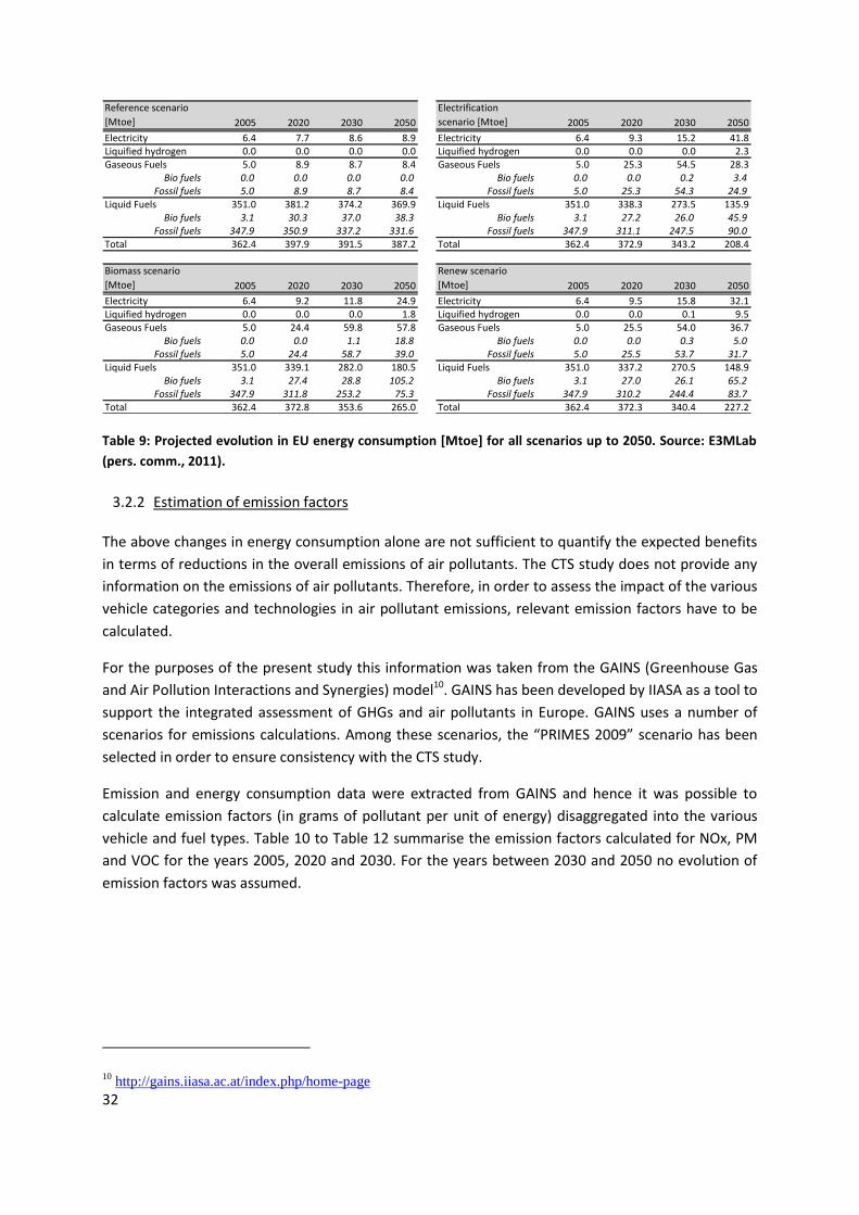


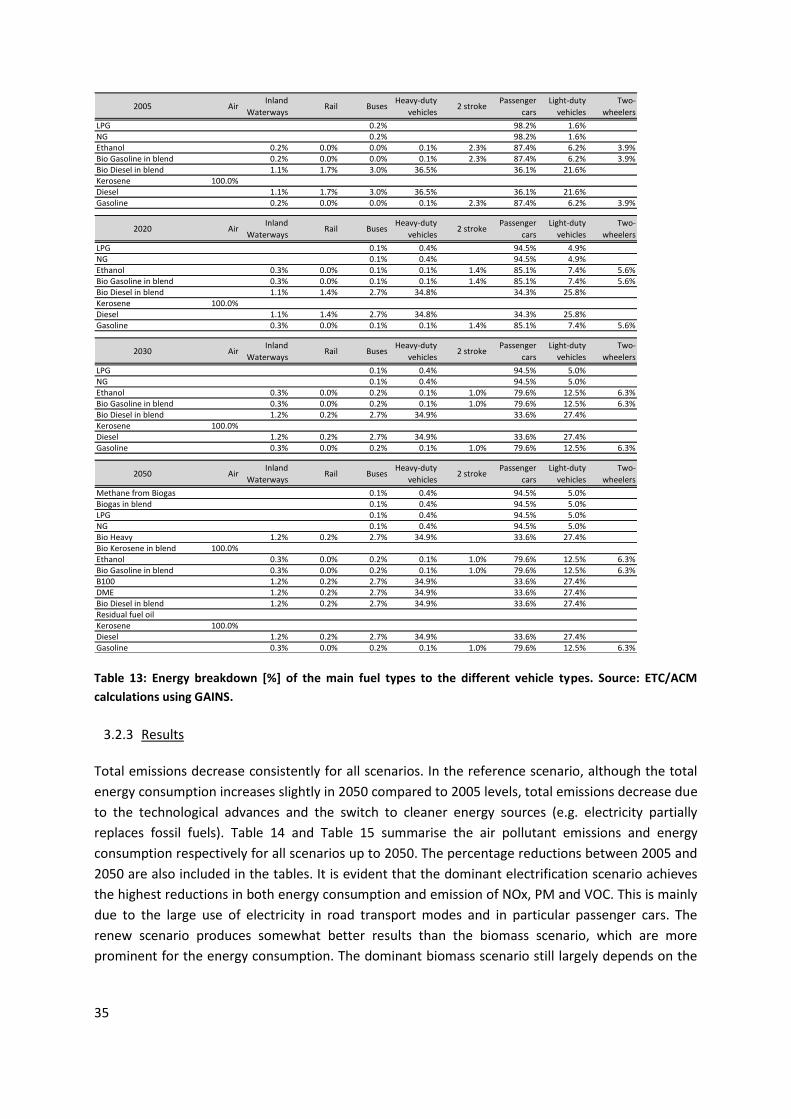

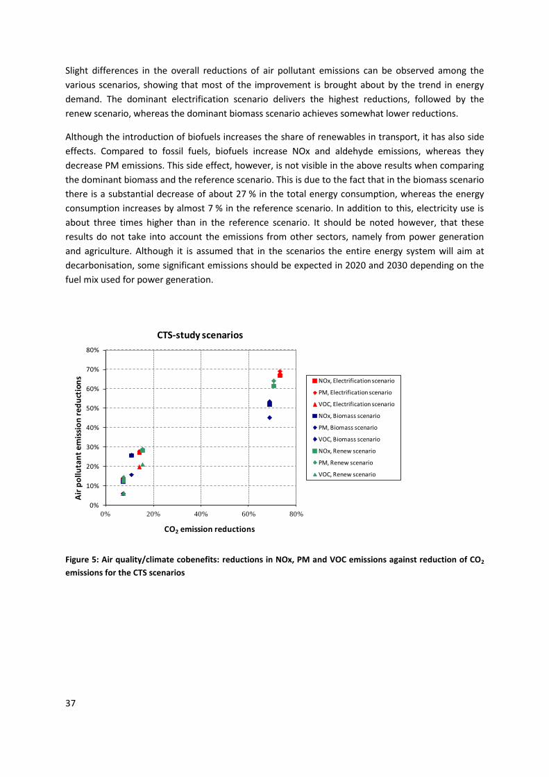


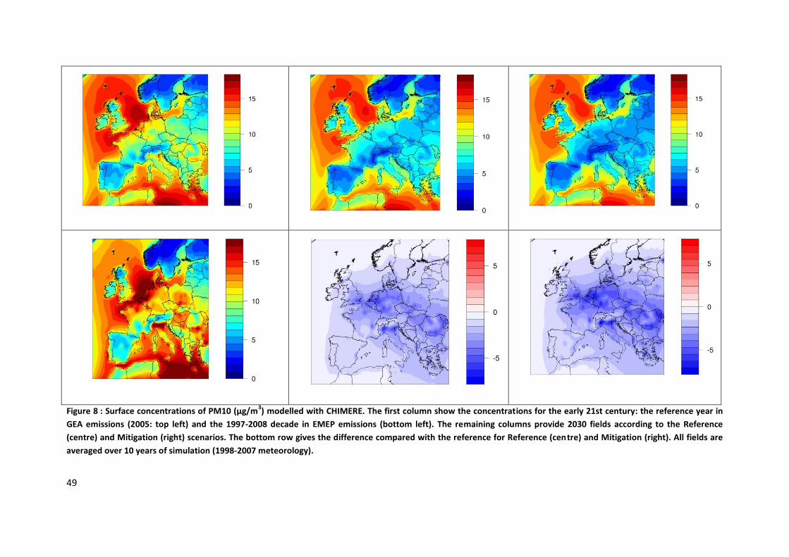


![Z u o ] W Y - Robert B. Laughlinlarge.stanford.edu/courses/2016/ph240/barber2/docs/gea-sep12.pdf · Are you a GEA member? What is GEA?: The Geothermal Energy Association (GEA) is](https://static.documents.pub/doc/80x56/5e814240a30c636ee277b2c6/z-u-o-w-y-robert-b-are-you-a-gea-member-what-is-gea-the-geothermal-energy.jpg)


