This discussion paper is/has been under review for the journal Hydrology and EarthSystem Sciences (HESS). Please refer to the corresponding final paper in HESSif available.
Combining remote sensing and GISclimate modelling to estimate daily forestevapotranspiration in a Mediterraneanmountain areaJ. Cristobal1,4, R. Poyatos2, M. Ninyerola1, P. Llorens3, and X. Pons4
1Department of Animal Biology, Plant Biology and Ecology, C-Building, Universitat Autonomade Barcelona, Cerdanyola del Valles, 08193, Spain2Center for Ecological Research and Forestry Applications (CREAF), Universitat Autonoma deBarcelona, Cerdanyola del Valles, 08193, Spain3Institute of Environmental Assessment and Water Research (IDÆA), CSIC, Jordi Girona, 18,Barcelona, 08034, Spain4Department of Geography, B-Building, Universitat Autonoma de Barcelona,Cerdanyola del Valles, 08193, Spain
Evapotranspiration monitoring allows us to assess the environmental stress on forestand agricultural ecosystems. Nowadays, Remote Sensing and Geographical Informa-tion Systems (GIS) are the main techniques used for calculating evapotranspiration atcatchment and regional scales. In this study we present a methodology, based on the5
energy balance equation (B-method), that combines remote sensing imagery with GISclimate modelling to estimate daily evapotranspiration (ETd) for several dates between2003 and 2005. The three main variables needed to compute ETd were obtained asfollows: (i) Land surface temperature by means of the Landsat-5 TM and Landsat-7ETM+ thermal band, (ii) air temperature by means of multiple regression analysis and10
spatial interpolation from meteorological ground stations data at satellite pass, and (iii)net radiation by means of the radiative balance. We calculated ETd using remote sens-ing data at different spatial and temporal scales (TERRA/AQUA MODIS and Landsat-5TM/Landsat-7 ETM+) and combining three different approaches to calculate the B pa-rameter. We then compared these estimates with sap flow measurements from a Scots15
pine (Pinus sylvestris L.) stand in a Mediterranean mountain area. This procedure al-lowed us to better understand the limitations of ETd modelling and how it needs to beimproved, especially in heterogeneous forest areas. The method using Landsat dataresulted in a good agreement, with a mean RMSE value of about 0.6 mm day−1 andan estimation error of ±30%. The poor agreement obtained using MODIS data reveals20
that ETd retrieval from coarse resolution remote sensing data is troublesome in theseheterogeneous areas, and therefore further research is necessary on this issue.
1 Introduction
Evaporation and transpiration are the two main processes involved in water transferfrom vegetated areas to the atmosphere. Evapotranspiration from the Earth’s vegeta-25
tion constitutes 88% of the total terrestrial evapotranspiration, and returns more than
50% of terrestrial precipitation to the atmosphere (Oki and Kanae, 2006); therefore itplays a key role in both the hydrological cycle and the energy balance of the land sur-face. Climate warming may accelerate the hydrological cycle as a result of enhancedevaporative demand in some regions where water is not limiting (Jung et al., 2010).However, the combination of warmer temperatures with constant or reduced precip-5
itation in other regions may lead to a large decrease in water availability for naturaland agricultural systems as well as for human needs (Jackson et al., 2001), especiallyin arid or semiarid areas (Jung et al., 2010) such as the Mediterranean Basin (Bateset al., 2008).
Evapotranspiration has been measured extensively at local scales using micromete-10
orological (such as eddy-covariance or the Bowen ratio) or sap flow techniques. Sincethe last decade, there have been several global initiatives to monitor evapotranspira-tion in different vegetation types, such as FLUXNET (Oak Ridge National LaboratoryDistributed Active Archive Center, 2010). Therefore, magnitudes and controls (climate,water availability, physiological regulation, etc.) on evapotranspiration are widely known15
for different types of vegetation, albeit at small spatial scales. How can we improve,then, our knowledge of evapotranspiration? In terms of spatial variability (and its driv-ing factors) the next challenge is larger scales.
ET can be modelled at global scales using GIS climate-based methodologies suchas GEPIC (Liu et al., 2007), LPJmL (Rost et al., 2008) or GCWM (Siebert and Doll,20
2010). However, radiometric measurements provided by remote sensing added to GISclimate regionalization have proved to be essential for modelling ET because they arethe only techniques that allow us to compute it feasibly at both regional (Cristobal et al.,2005; Kustas and Norman, 1996) and global scales (Mu et al., 2007). Moreover, theuse of remote sensing techniques supplements the frequent lack of ground-measured25
variables and parameters that are required for applying the local models at a regionalscale (Sanchez et al., 2008a).
Currently, there are a wide variety of remote sensing models for calculating ET atglobal or regional scales, such as METRIC (Allen et al., 2007), SEBAL (Bastiaanssenet al., 1998), TSEB (Kustas and Norman, 2000), ALEXI/disALEXI (Anderson et al.,2004), S-SEBI (Roerink et al., 2000), STSEB (Sanchez et al., 2008) and the B-method(Jackson et al., 1977; Seguin and Itier, 1983); other methodologies can be found in5
Schmugge et al. (2002). All these theoretical methods used to estimate ET at a regionalscale with remote sensing techniques are derived from the energy balance equationbased on the principle of energy conservation in a system formed by soil and vege-tation. Most of them try to minimize the inputs from ancillary data (often data fromground meteorological stations) in order to make the algorithms more operational at10
global scales. However, there is currently no agreement on which method is the mostappropriate because this often depends on the application purposes (Sanchez et al.,2008a).
Most of these methods have been validated in homogeneous covers (crops or naturalvegetation) and flat areas, where a single meteorological station record is used to15
describe the climate conditions of a large area. In these areas, the use of mediumor coarse spatial resolution remote sensing data is enough to obtain accurate dailyET (ETd) results. However, in more complex and heterogeneous areas, due to thelandscape, orographic or climatic variability, a single meteorological record or remotesensing data with coarse spatial resolution may not be accurate enough to calculate20
the ETd. Operative GIS climate-based techniques can be used at regional scales inboth simple and complex areas (Ninyerola et al., 2007; Pons and Ninyerola, 2008)to achieve higher accuracy and provide the input variables for agriculture and naturalvegetation evapotranspiration modelling.
The objective of this paper is to validate with Scots Pine (Pinus sylvestris L.) stand-25
scale sap flow measurements a simple method to compute daily ET in a heteroge-neous Mediterranean mountain area during a three year period. GIS climate-basedregional modelling was used instead of a single meteorological measurement to obtainthe meteorological inputs (air temperature and solar radiation) in order to evaluate the
performance of this technique. Low (TERRA/AQUA MODIS) and medium (Landsat-TM/ETM+) spatial resolution remote sensing images were used as the remote sensinginputs in order to evaluate their accuracy in a heterogeneous landscape.
2 Data and methods
2.1 Study area5
The study plot is located within the Vallcebre research catchments (Gallart et al., 2005;Latron et al., 2010; Llorens et al., 2010), 42◦12′ N, 1◦49′ E, located in the Eastern Pyre-nees (NE Iberian Peninsula). It has a humid Mediterranean climate, with a markedwater deficit in summer. The mean annual temperature at 1260 m is 9.1 ◦C, and thelong term (1983–2006) mean annual precipitation is 862±206 mm, with a mean of 9010
rainy days per year. The long term (1989–2006) mean annual reference evapotranspi-ration, calculated using the Hargreaves and Samani (1982) method, was 823±26 mm.Mudstone and limestone substrates are predominant, resulting in clayey soils in thefirst case, and bare rock areas or thin soils in the latter (Gallart et al., 2002). The veg-etation in the area is sub-Mediterranean oak forest (Buxo-sempervirentis-Quercetum15
pubescentis association), but most of the land was terraced and deforested for cul-tivation in the past, and then progressively abandoned during the second half of thetwentieth century. The present landscape is mainly a mosaic of mesophylous grass-lands and patches of Scots Pine, which colonized old agricultural terraces after theywere abandoned (Poyatos et al., 2003). Figure 1 shows the location of the Vallcebre20
research catchments.
2.2 Meteorological and remote sensing data
We used two sources of meteorological data to fit and validate the models. In thecase of the Scots Pine stand, air temperature, wind speed and net radiation data were
recorded every 10 s by means of HMP35AC (Vaisala, Vantaa, Finland), A100R (VectorInstrumentsRhyl, UK) and NR-Lite (Kipp & Zonen, Delft, The Netherlands) sensors, re-spectively, and stored as 15-min average in a data logger, DT500, DataTaker, Australia(Poyatos et al., 2005).
In the case of air temperature and net radiation regionalization, meteorological data5
from 161 meteorological stations were downloaded from the Catalan MeteorologicalService (SMC) web (meteorological data available at http://www.meteocat.com). Fig-ure 1 shows the spatial distribution of these two sources of meteorological data.
A set of 30 TERRA-MODIS images and 27 AQUA-MODIS images and a set of 11Landsat-7 ETM+ and 10 Landsat-5 TM images from paths 197 and 198, row 31 were10
selected to perform the ETd modelling of the Scots Pine forest stand from 2003 to 2005.Figure 2 shows the temporal distribution of the selected dates aggregated by month.
AQUA/TERRA MODIS images were downloaded with the Land ProcessesDistributed Active Archive Center gateway (https://wist.echo.nasa.gov/∼wist/api/imswelcome/). We selected three different types of products which contain the remote15
sensing data we used to calculate the ETd: MOD11A1 and MYD11A1 (which containTERRA and AQUA daily land surface temperature, LST, and emissivity, respectively),MOD09GHK and MYD09GHK (which contain TERRA and AQUA daily reflectances,respectively), and MOD05 (which contains daily water vapour). Although image timeacquisition is different for each satellite, Landsat and TERRA satellites pass over Cat-20
alonia at a similar time, between 09:30 and 10:30 LST (local solar time). AQUA passesover the same area, but between 13:00 and 14:00 LST.
2.3 The evapotranspiration model
We used the B-method to compute ETd. This methodology is derived from the modelproposed by Jackson et al. (1977), which is based on the energy balance equation25
and has been used or modified for both natural vegetation and crop areas by differentauthors (Caselles et al., 1992, 1998; Garcıa et al., 2007; Sanchez et al., 2007, 2008a,Seguin and Itier, 1983; Vidal and Perrier, 1989). Seguin and Itier (1983) proposed
a modified equation that needs net radiation (Rn) and the difference between LST andair temperature at satellite pass (Ti) as input variables :
ETd =Rnd−B(LST−Ti)n (1)
where subindex d is the daily periods, ET and Rn are in mm day−1 and both tempera-tures are in K. Exponent n is a correction for non-neutral static stability that could be5
assigned to one, as Seguin and Itier (1983) suggested. Due to the importance of theB parameter in calculating ETd, we used two approaches to compute B.B can be defined as an exchange coefficient that in Eq. (1) represents an average
bulk conductance for the daily-integrated sensible heat flux. This term is related to thesensible heat flux (H), one of the most difficult variables to determine in the energy10
balance equation (Bastiaanssen et al., 1998). There are several approaches that useLST directly, such as the parallel resistance model developed by Norman et al. (1995),and the one developed by Caselles et al. (1992), which is adapted for heterogeneousareas and defined by the following equation:
B=(Rnd
Rni
)∗(
ρCp
r∗a
)(2)15
where subindex i means instantaneous and (Rnd/Rni) is called the Rn ratio. ρCp is
the volumetric heat capacity of air (J kg−1 K−1) and r∗a is the effective aerodynamicresistance. Measurements of effective aerodynamic resistance are not usually easy toobtain; therefore, we considered the aerodynamic resistance of Pinus sylvestris to beequal to 28.1 m s−1, as determined by Sanchez et al. (2007), because our study area20
is similar to that of this previous work (Dr. Sanchez, personal communication, 2009).In addition, B can also be obtained using the simple equation proposed by Carlson
et al. (1995), obtained from a soil-vegetation atmosphere transfer model that integratesthe main factors on which B depends, such as wind velocity and aerodynamic resis-tance; therefore, B can also be defined as:25
where NDVI∗ is a scaled vegetation index based on the NDVI and is defined as:
NDVI∗ =NDVIp−NDVI0NDVIs−NDVI0
(4)
where subindex p is the image NDVI value for a given pixel, 0 is a bare soil pixel and sis a fully vegetated pixel.
2.4 ETd model inputs5
2.4.1 Landsat and TERRA/AQUA image processing
Landsat images were corrected by means of conventional techniques based on firstorder polynomials. The effect of the relief of the land surface was taken into accountby using a digital elevation model (Pala and Pons, 1995), and a mean RMSE less than15 m was obtained. Radiometric correction was carried out following the methodology10
proposed by Pons and Sole-Sugranes (1994), which allows us to reduce the numberof undesired artifacts due to the atmospheric effects or differential illumination that areresults of the time of day, the location on the Earth and the relief (zones being moreilluminated than others, shadows, etc). The digital numbers were converted to radi-ances by means of image header parameters, taking into account the considerations15
presented by Cristobal et al. (2004) and Chander et al. (2009).Given that AQUA/TERRA MODIS reflectance and LST and emissivity products
are corrected geometrically and radiometrically by USGS, these products were onlyimported, with all the necessary metadata to process them. Before that, im-ages were reprojected to UTM-31 N. The water vapour product was geometrically20
corrected using HEG-WIN software (http://newsroom.gsfc.nasa.gov/sdptoolkit/HEG/HEGDownload.html).
Different air temperature input variables are needed to compute net radiation LST andETd: satellite pass air temperature (Ti), daily mean air temperature (Ta) and daily mini-mum air temperature (Tmin). To regionalize air temperature, we applied multiple regres-sion analysis combined with spatial interpolation techniques (Cristobal et al., 2008;5
Ninyerola et al., 2000, 2007). Air temperature data were fitted using 60% of the me-teorological ground stations and cross-validated with the remaining 40%. In theseprevious works, Ti, Ta and Tmin were obtained with an RMSE of 1.8 K, 1.3 K and 2.3 K,respectively.
2.4.3 Land surface temperature (LST) and emissivity (LSE)10
In the case of Landsat-5 TM and Landsat-7 ETM+, the LST was calculated with themethodology proposed by Cristobal et al. (2009), which is based on the radiativetransfer equation and needs air temperature and water vapour as input variables. Ityielded a RMSE of about 1 K. The methodology is designed for a wide range of watervapour values (0 to 8 g cm−2) to take into account global conditions. The TERRA/AQUA15
MODIS water vapour product (MOD05) was used as the water vapour source. The airtemperature was computed as explained in Sect. 2.4.2.
To compute LSE we used the NDVI threshold method proposed by Sobrino and Rais-souni (2000) and Sobrino et al. (2008). This methodology uses certain NDVI thresholdsto distinguish between bare soil, fully vegetated and mixed pixels. According to the au-20
thors it gives an error of 1% (Sobrino et al., 2008).
2.4.4 Net radiation (Rn)
Daily net radiation was computed with the energy balance equation as follows:
where α is the surface albedo, Rs↓ is the incoming short wave radiation, Ta is the airtemperature; σ is the Stephan-Boltzmann constant; ε is the surface emissivity and εais the air emissivity.
The first term of Eq. (5), Rs↓·(1−α), refers to daily incoming shortwave radiation. Inthis case, albedo (α) was computed using the Liang (2001) methodology in the case of5
Landsat- 5 TM and Landsat-7 ETM+ images, and the method by Liang et al. (1999) inthe case of TERRA/AQUA MODIS images. Both methodologies use a weighted sumof visible, near infrared and medium infrared radiation, and according to the authorsthe error in estimating albedo is less than 2%. Daily solar radiation (Rs↓) was obtainedwith the methodology proposed by Pons and Ninyerola (2008). Given a digital elevation10
model, we can calculate the incident solar radiation at each point during a particularday of the year taking into account the position of the Sun, the angles of incidence,the projected shadows, the atmospheric extinction and the distance from the Earth tothe Sun at fifteen minute intervals. The diffuse radiation was estimated from the directradiation and the exoatmospheric direct solar irradiance was estimated with the Page15
equation (1986) that Baldasano et al. (1994) fitted with information from Catalonia.The second term of Eq. (5) refers to daily incoming longwave radiation. This termhas been approximated using the methodology proposed by Dilley and O’Brien (1998),which according to the authors obtains an RMSE of 5 W m−2 and an R2 of 0.99 inits computation. The third term of Eq. (5) refers to daily outgoing longwave radiation.20
This term was approximated with the methodology proposed by Lagouarde and Brunet(1993).
2.4.5 B parameter
As we explained in Sect. 2.3, B parameter was calculated with two approaches: the Rnratio and NDVI. In the Rn ratio approach, we used two ways to compute the parameter:25
(1) a regional Rn ratio (hereafter referred to as the B-Rn ratio regional) with data from13 meteorological stations of the SMC meteorological network, and Eq. (2) a local Rnratio (hereafter referred to as the B-Rn ratio local) with data from the meteorological
station above the Scots Pine stand in the Vallcebre research catchments. We usedthese two data sources to evaluate whether a regional measurement of the Rn ratioprovides similar results as a local measurement.
In the NDVI approach (hereafter referred to as the B-NDVI), Carlson et al. (1995)suggested selecting NDVI values depending on the study area. In our case, bare soil5
and fully vegetated NDVI values were set to 0.1 and 0.7 for the entire dataset, as thesevalues were realistic enough to simulate bare soil and full vegetation conditions overthe study area.
2.5 Sap flow measurements and upscaling to stand transpiration
We compared remote sensing daily evapotranspiration estimates with sap flow mea-10
surements upscaled to stand transpiration. Sap flow density in the outer xylem wasmeasured with 20 mm long heat dissipation probes constructed according to Granier(1985). Sap flow gauges were installed at breast height on the north-facing side of12 Scots Pine trees and were covered with reflective insulation to avoid the influenceof natural temperature gradients in the trunk. The sap flow density measured by heat15
dissipation probes was corrected for radial variability in sap flow using correction coef-ficients derived from radial patterns of sap flow within the xylem measured with a multi-point heat field deformation sensor (Nadezhdina et al., 2002). A gravimetric analysisof wood cores was carried out to estimate sapwood depths in a sample of Scots Pinetrees, and a linear regression was obtained between the basal area and sapwood area20
of individual trees. Stand transpiration was then calculated by multiplying the averagesap flow density within a diametric class by the total sapwood area of trees in thatclass. Further details on the methodology and results of sap flow measurements usedin this study can be found in Poyatos et al. (2005, 2008).
The B parameter showed different behaviour depending on the approach used. TheB-Rn ratio local had a mean and standard deviation (s.d.) of 6.9 and 3.2 Wm−2, re-spectively, in the case of Landsat dates (see Fig. 2), and a mean and s.d. of 10.85
and 2.2 Wm−2, respectively, in the case of TERRA/AQUA dates. The B-Rn ratio re-gional displayed a mean and s.d. of 9.5 and 2.3 Wm−2, respectively, in the case ofLandsat dates, and a mean and s.d. of 12.8 and 2.4 Wm−2, respectively, in the caseof TERRA/AQUA dates. Finally, B-NDVI showed a mean and σ of 11.9 and 2.6 Wm−2,respectively, in the case of Landsat dates, and a mean and σ of 12.6 and 2.6 Wm−2,10
respectively, in the case of TERRA/AQUA dates.B-NDVI was similar in Landsat and TERRA/AQUA dates, but not in the B approach
using the Rn ratio, especially in the case of the B-Rn ratio local. While on winter andautumn dates the B-Rn ratio local had small values (positive or negative) close to 0,B-NDVI tended to show higher positive values. For example, B computed on 11 Jan-15
uary 2005, using the Rn local ratio gave a negative value close to 0 Wm−2, whereasin the case of B-NDVI it was 11.8 Wm−2. During these seasons we would expect lowB values due to the energy budget; therefore, this suggests that B-NDVI could be lesssensitive in winter and autumn situations than the B-Rn ratio.
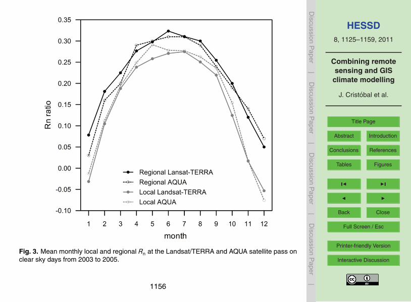
In the case of the B-Rn ratio, the Rn ratio is usually obtained from a net radiation20
sensor over the study area. Some authors have used a constant value of 0.3±0.02(Seguin and Itier, 1983; Kustas et al., 1990; Garcıa et al., 2007) because most of thedates used in these studies were in spring or summer and over crop areas. However,we found that our local (Vallcebre research catchments) and regional (SMC meteoro-logical stations) Rn ratios varied over the year (see Fig. 3). The Rn local and regional25
ratios for the Landsat/TERRA satellite pass had an annual mean (from 2003 to 2005period) of 0.16±0.05 (mean and s.d.) and 0.22±0.03, respectively, and in the case
of the AQUA satellite pass, an annual mean of 0.17±0.05 and 0.21±0.02, respec-tively. In addition, the Rn ratio varied little from 09:00 to 14:00 LST in our study area,and thus was useful in Landsat and TERRA/AQUA ETd modelling. Therefore, we useda daily Rn ratio instead of a constant Rn ratio. This is in agreement with other authorswho also reported a similar Rn ratio behaviour (Sanchez et al., 2007; Sobrino et al.,5
2005; Wassenaar et al., 2002). Rn ratio values reported in these studies are similarto the regional Rn ratio computed in our study area because our value was obtainedat meteorological stations at a similar altitude as those in the literature. However, thelocal Rn ratio values are lower, which shows that this ratio does not only vary with lati-tude as Sanchez (2007) suggests, but also with altitude. Further research into Rn ratio10
modelling in mountainous areas is therefore needed.Moreover, it is worth remarking that the local Rn ratio obtained in the Scots Pine stand
displayed a different pattern to the regional Rn ratio because it had negative valueson winter days when the Rn budget is negative, which often occurs in mountainousareas (Barry, 2001). ETd models do not usually predict this situation because they are15
generally applied in spring and summer and in relatively flat and low altitude areas.
3.2 Net radiation validation
The results show a good agreement between the Rnd measured in the Scots Pinestand and the Rnd obtained using the Landsat regional model with an R2 of 0.89 andan RMSE of 22 Wm−2 (see Table 1). The Rnd derived from TERRA/AQUA MODIS20
showed a similar RMSE but lower R2 (0.77 and 0.73, respectively; Table 2). It is worthnoting that the proposed Rnd model developed with regional variables, such as Rs↓,LST and Ta, makes it possible to approximate this variable over large areas with a highlevel of accuracy.
In the ETd validation, we obtained a test R2 of 0.84 when the B parameter was esti-mated using a regional Rn ratio computed with the SMC meteorological stations (B-Rnratio regional), 0.84 when the B parameter was estimated using a local Rn ratio com-5
puted with the Scots pine stand meteorological station (B-Rn ratio local), and 0.82 whenthe B parameter was estimated using the NDVI approach, B-NDVI. It is interesting tonote that for the ETd models used, the minimum values were always negative. Thismainly happens on winter dates when the Rn ratio is also negative. Therefore, on win-ter dates this methodology should only be used on days when the Rn budget is positive.10
Errors close to 1 mm day−1 were obtained for the RMSE. Taking into account the rangeof ETd values observed in the studied Scots Pine stand (from 0.5 to 2.7 mm day−1), wecannot conclude that the model provides optimal results. When the Rnd ratio is nega-tive during winter, the ETd yields negative values and the model does not perform well.Again, it is worth noting that ETd models are usually validated on spring or summer15
dates (Chiesi et al., 2002; Nagler et al., 2005, 2007; Sanchez et al., 2007, 2008; Ver-straeten et al., 2005; Wu et al., 2006) when the daily Rn budget is positive. Our attemptto also estimate ETd during autumn and winter has shown the limitations of the methodand how ETd modelling needs to be further improved, especially in forest areas.
We obtained a better mean RMSE for the different models when only those dates20
with a positive Rnd ratio were selected, which ranged from 0.5 to 0.7 mm day−1 witha similar R2 (see Tables 2–3 and Fig. 4). Of the different approaches used to computethe B parameter, the best results were obtained using the local Rn ratio and the NDVIapproaches, with a RMSE of 0.5 and 0.6 mm day−1, respectively, and an estimationerror of about ±30%. Indeed, the regional Rn ratio yielded a higher RMSE and estima-25
tion error of about 0.7 mm day−1 and ±38%, respectively; this could be explained bythe differences in the Rn ratio estimation. The regional Rn ratio was computed from the
data from the SMC meteorological stations, which are designed for crop assessmentand are located in areas at low to medium heights (from 0 to 500 m). Our study areais located at 1250 m; therefore, the regional Rn ratio conditions are not representativeof our study area. However, it is important to note that optimal Rn ratio values are dif-ficult to obtain because it would be necessary to have a meteorological network with5
Rn instruments distributed at different altitudes in diverse landscapes. Moreover, Rninstruments are usually found in agrometeorological networks but not very often overforest areas. Although the two B parameter approaches (B-Rn ratio local and B-NDVI)obtained similar results, we have to take into account that the main disadvantage of theNDVI approach is the subjectivity involved in adopting the NDVI thresholds to compute10
NDVI∗. However, if a well-balanced regional Rn ratio is not available due to limitationsin the meteorological networks, the NDVI approach is preferable for computing the Bparameter at regional scales. In all cases, the models tended to overestimate ETd,showing higher values in the case of the regional Rn ratio and lower values in the caseof the NDVI approach.15
In this study, we are strictly comparing evapotranspiration with stand transpiration ofthe dominant tree species. As the understory in the studied stand is very poor, the onlyother contribution comes from soil evaporation, with typical rates of 0.1 to 0.5 mm day−1
(Poyatos et al., 2007). These values are consistent with the systematic bias betweensap flow-derived transpiration and the ETd models (see Fig. 4).20
In addition, it should be stressed that the difficulty of obtaining the effective aerody-namic resistance and the use of a constant value for the analyzed period may haveintroduced more variability into our analysis, and thus increased the error in the ETdmodels.
3.3.2 TERRA/AQUA MODIS25
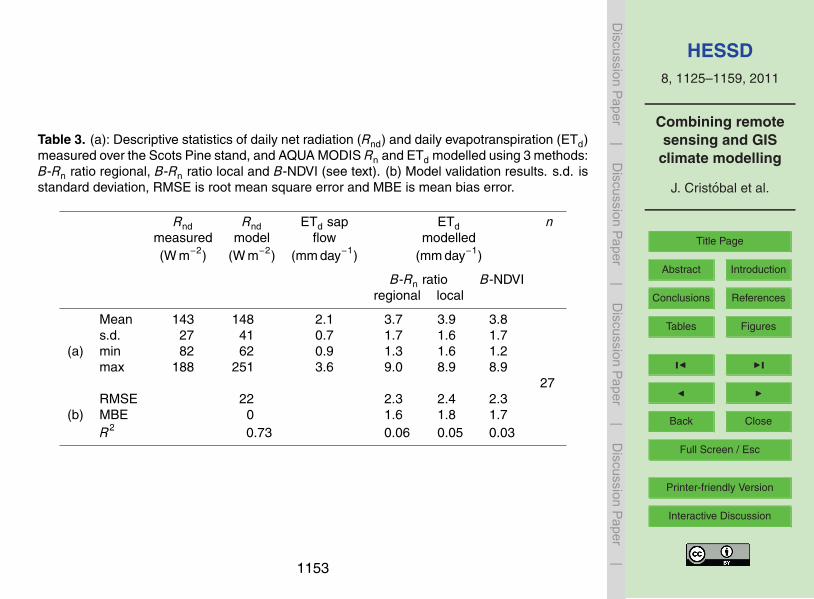
TERRA and AQUA ETd validation did not obtain the same results as Landsat (seeTables 2–3 and Figs. 5–6). In both cases, ETd validation showed a higher RMSE,between 1.8 and 2.4 mm day−1, and a low R2, between 0.03 and 0.07. Despite air
temperature models also showing good validation results, one possible source of erroris the LST. Therefore, it seems that although TERRA/AQUA MODIS LST provides goodresults in Rnd modelling, this is not the case in ETd modelling.
The study area does not cover a 1000 m×1000 m pixel, and therefore the remotesensing data, especially the LST, is less representative than a Landsat pixel of 605
(ETM+) or 120 m (TM). As we mentioned in Sect. 2.1, the study area has high spatialheterogeneity (mosaic of afforestation patches overgrowing old agricultural terraces)at smaller scales than the coarse TERRA/AQUA MODIS pixel, which makes it diffi-cult to validate the ETd model results. However, it has to be noted that validatinga TERRA/AQUA MODIS in a heterogeneous mountain landscape is not easy due to the10
extensive instrumentation needed to measure the energy flux in each of the landscapecovers. Therefore, it seems that the use of TERRA/AQUA MODIS images themselvesin this type of landscape is not enough to accurately map ET on a daily basis. In orderto improve the ETd results using coarse resolution images, downscaling techniquessuch as those in Anderson et al. (2004) are required.15
There are very few studies in the literature that monitor ETd at both high spatial andtemporal resolutions during an annual period in a forest area, especially using a largenumber of Landsat images. In addition, most of the studies to date have dealt with en-vironments subjected to only mild water stress, such as riparian forests, crops or borealstands. For example, Wu et al. (2006) reported an RMSE of 0.6 mm day−1 in a tropical20
forest using only one Landsat image. They compared their results with estimates fromthe literature due to the difficulty in validating these kinds of regions using sap flowmeasurements. Nagler et al. (2005, 2007) modelled ETd using 8 Landsat-5 TM andabout 90 MODIS dates in a cottonwood plantation in riparian corridors of the WesternUS during the July-August period in 2005, and obtained an uncertainty in modelled25
ETd of 20–30%. Verstraeten et al. (2005) also reported an uncertainty of about 27% ininstantaneous ET modelled with NOAA-imagery and validated using EUROFLUX dataduring the growing seasons of European forests, from March to October. Sanchezet al. (2007) modelled ETd using MODIS in a homogeneous Pinus sylvestris stand
in the boreal region, and reported an RMSE of 0.81 mm day−1 and an uncertainty ofabout 30% in ETd compared to eddy-covariance data. With a more demanding methodin terms of ancillary data needs, FOREST-BGC, Chiesi et al. (2002) reported a meanRMSE of 0.4 mm day−1 introducing LAI derived from 10-day composites of NOAA im-ages in two oak stands. More recently, Sanchez et al. (2008a) obtained a value of5
0.7 mm day−1 in different coniferous, broad-leaf and mixed forests in the Basilicata re-gion with three Landsat-5 TM and ETM+ images from spring and summer.
Overall, for Landsat ETd modelling, our results are in agreement with the studies inthe literature, as we obtained an uncertainty of about 30%. One positive point of theresults of the Landsat ETd models across different seasons is the robust ETd estimation10
under varied conditions of water availability, as the studied stand undergoes differentdegrees of water stress in spring, summer and autumn (Poyatos et al., 2008). However,in the case of MODIS ETd modelling, the validation shows a higher RMSE, whichsuggests that higher spatial resolution is needed for heterogeneous areas.
In addition, it is worth noting that implementing regional models for calculating Ta,15
LST and Rs↓, as inputs in both Rn and ETd modelling has provided good results andmade it possible to compute these variables at regional scales with similar accuracy tothat in the literature.
It is important to note, however, that we have found some limitations in ETd modellingin a mountainous forested area that should be addressed in the future in order to moni-20
tor this variable in an operational way. Further work to improve the described methodol-ogy should include: (i) The validation of a multi-scale remote sensing model (Andersonet al., 2004) for disaggregating regional fluxes to micrometeorological scales. Thiswould allow ETd to be monitored on a daily basis instead of on a 16-day basis thanksto the TERRA/AQUA temporal resolution; (ii) The implementation of methodologies for25
calculating aerodynamic resistance, such as those described by Norman et al. (1995)and Sanchez et al. (2008a,b).
The B-method has been used to estimate daily evapotranspiration (ETd) in a ScotsPine stand in a mountainous Mediterranean area, obtaining an estimation error of±30% (corresponding to 0.5–0.7 mm day−1) using medium spatial resolution imagery,Landsat-5 TM and Landsat-7 ETM+, and the different approaches presented. These5
results are in agreement with recent studies that used a similar spatial resolution.However, when lower spatial resolution was used (TERRA/AQUA MODIS) the resultsshowed larger errors, 1.9 and 1.7 mm day−1, respectively.
The Rn ratio emerged as an important parameter to be considered when the B-method is used. Although this ratio is close to 0.3 in spring and summer months, this10
value is not appropriate for winter and autumn because when the Rn ratio is negative(negative Rn budget) the B-method does not provide a realistic ETd. Further researchis therefore needed to estimate this parameter in these conditions.
The best ETd results were obtained using a local Rn ratio approach to calculate the Bparameter, followed by the method using NDVI. The regional Rn ratio resulted in larger15
errors, which means that if a well balanced meteorological network (with Rn sensors)is not available, the NDVI approach is preferable for calculating the B parameter ata regional scale.
Regional ETd models for calculating input variables, such as Rs↓, LST and Ta, per-formed well, making it possible to compute ETd at a regional scale with a good level of20
accuracy.Finally, using a large number of remote sensing images that are well distributed over
the analyzed period, especially in the case of Landsat, allowed us to better understandthe limitations of the methodologies and how to address the further improvement ofETd modelling, especially in forest areas.25
Acknowledgements. The authors would like to thank our colleagues of the Research Group ofMethods in Remote Sensing and GIS (GRUMETS) who collaborated in several ways in imagetreatment, and Juan Manuel Sanchez from the Department of Earth Physics and Thermody-namics of the University of Valencia for his help in evapotranspiration modelling, and to ourcolleagues of the Surface Hydrology and Erosion Group – IDAEA for their help in field data5
acquisition. It would not have been possible to carry out this study without the financial supportof the Ministry of Science and Innovation and the FEDER funds through the research project“SCAITOMI (TIN2009-14426-C02-02)”. The Catalan Government provided funding to our Re-search Group for Methods and Applications in Remote Sensing and Geographic InformationSystems – “GRUMETS (2009SGR1511)”, and “MONTES (CSD2008-00040)”. We would like10
to express our gratitude to the Catalan Water Agency and to the Ministry of the Environmentand Housing of the Generalitat (Autonomous Government of Catalonia) for their investmentpolicy and the availability of Remote Sensing data, which has made it possible to conduct thisstudy under optimal conditions. Xavier Pons is recipient of an ICREA Academia Excellence inResearch grant.15
References
Allen, R. G., Tasumi, M., and Trezza, R.: Satellite-based energy balance for mapping evap-otranspiration with internalized calibration (METRIC)-Model, J. Irrig. Drain. E.-ASCE, 133,395–406, 2007.
Anderson, M. C., Norman, J. M., Mecikalski, J. R., Torn, R. D., Kustas, W. P., and Basara, J. B.:20
A multi-scale remote sensing model for disaggregating regional fluxes to micrometeorologicalscales, J. Hydrometeorol., 5, 343–363, 2004.
Anderson, M. C., Kustas, W. P., and Norman, J. M.: Upscaling flux observations from local tocontinental scales using thermal remote sensing, Agron. J., 99, 240–250, 2007.
Baldasano, J. M., Calbo, J., and Moreno, J.: Atlas de Radiacio Solar a Catalunya (Dades del25
perıode 1964–1993), Institut de Tecnologia i Modelitzacio Ambiental (ITEMA), UniversitatPolitecnica de Catalunya, Terrassa, 1994.
Barry, R. E.: Mountain Weather and Climate, 2nd edition, Routledge, Taylor and Francis Group,London, 2001.
Bates, B. C., Kundzewicz, Z. W., Wu, S., and Palutikof, J. P.: Climate Change and Water, Tech-nical Paper of the Intergovernmental Panel on Climate Change, IPCC Secretariat, Geneva,2008.
Bastiaanssen, W. G. M., Meneti, M., Feddes, R. A., and Holtslag, A. A. M.: A remote sensingsurface energy balance algorithm for land (SEBAL), 1. Formulation, J. Hydrol., 212–213,5
198–212, 1998.Carlson, T. N., Caphart, J., and Gillies, R. R.: A new look at the simplified method for remote
sensing of daily evapotranspiration, Remote Sens. Environ., 54, 161–167, 1995.Caselles, V., Sobrino, J. A., and Coll, C.: On the use of satellite thermal data for determining
evapotranspiration in patially vegetated areas, Int. J. Remote Sens., 13, 2669–2682, 1992.10
Caselles, V., Artiago, M. M., and Hurtado, E.: Maping actual evapotranspiration by combin-ing Landsat and NOAA-AVHRR images: application to the Barrax area, Albacete, Spain,Remote Sens. Environ., 63, 1–10, 1998.
Chander, G., Markham, B. L., and Helder, D. L.: Summary of current radiometric calibrationcoefficients for Landsat MSS, TM, ETM+, and EO-1 ALI sensors, Remote Sens. Environ.,15
113, 893–903, 2009.Chiesi, M., Maselli, F., Bindi, M., Fibbi, L., Bonora, L., Raschi, A., Tognetti, R., Cermak, J., and
Nadezhdina, N.: Calibration and application of FOREST-BGC in a Mediterranean area bythe use of conventional and remote sensing data, Ecol. Model., 154, 251–262, 2002.
Cristobal, J., Pons, X., and Serra, P.: Sobre el uso operativo de Landsat-7 ETM+ en Europa,20
Rev. Teledeteccion, 21, 55–59, 2004.Cristobal, J., Pons, X., and Ninyerola, M.: Modelling actual evapotranspiration in Catalonia
(Spain) by means of remote sensing and geographical information systems, Gottinger Geogr.Abh., 113, 144–150, 2005.
Cristobal, J., Ninyerola, M., and, X. Pons: Modelling air temperature through a combination of25
Remote Sensing and GIS data, J. Geophys. Res., 13, D13106, 1–13, 2008.Cristobal, J., Jimenez-Munoz, J. C., Sobrino, J. A., Ninyerola, M., and Pons, X.: Improvements
in land surface temperature retrieval from the landsat series thermal band using water vapourand air temperature, J. Geophys. Res., 114, D08103, 1–16, 2009.
Dilley, A. C. and O’Brien, D. M.: Estimating downward clear sky long-wave irradiance at the30
surface from screen temperature and precipitable water, Q. J. Roy. Meteor. Soc., 124, 1391–1401, 1998.
Gallart, F., Llorens, P., Latron, J., and Regues, D.: Hydrological processes and their seasonalcontrols in a small Mediterranean mountain catchment in the Pyrenees, Hydrol. Earth Syst.Sci., 6, 527–537, doi:10.5194/hess-6-527-2002, 2002.
Garcıa, M., Villagarcıa, L., Contreras, S., Domingo, F., and Puigdefabregas, J.: Comparison ofthree operative models for estimating the surface water deficit using ASTER reflective and5
thermal data, Sensors, 7, 860–883, 2007.Giorgi, F., Bi, X. Q., and Pal, J.: Mean interannual variability and trends in a regional climate
Granier, A.: Une nouvelle methode pur la mesure du flux de seve brute dans le tronc des10
arbres, Ann. Sci. Forest, 42, 193–200, 1985.Hargreaves, G. H. and Samani, Z. A.: Estimating potential evapotranspiration, J. Irr. Drain.
Div.-ASCE, 108, 225–230, 1982.Jackson, R. B., Carpenter, S. R., Dahm, C. N., McKnight, D. M., Naiman, R. J., Postel, S. L.,
and Running, S. W.: Water in a changing world, Ecol. Appl., 11, 1027–1045, 2001.15
Jackson, R. D., Reginato, R. J., and Idso, S. B.: Wheat canopy temperature: a practical tool forevaluating water requirements, Water Resour. Res., 13, 651–656, 1977.
Jung, M., Reichstein, M., Ciais, P., Seneviratne, S. I., Sheffield, J., Goulden, M. L., Bonan, G.,Cescatti, A., Chen, J., Jeu, R., Dolman, A. J., Eugster, W., Gerten, D., Gianelle, D., Gob-ron, N., Heinke, J., Kimball, J., Law, B. E., Montagnani, L., Mu, Q., Mueller, B., Oleson, K.,20
Papale, D., Richardson, A. D., Roupsard, O., Running, S., Tomelleri, E., Viovy, N., Weber, U.,Williams, C., Wood, E., Zaehle, S., and Zhang, K.: Recent decline in the global land evapo-transpiration trend due to limited moisture supply, Nature, 467, 951–954, 2010.
Kustas, W. P. and Norman, J. M.: Use of remote sensing for evapotranspiration monitoring overland surfaces, Hydrolog. Sci. J., 41, 495–516, 1996.25
Kustas, W. P. and Norman, J. M.: A two-source energy balance approach using directionalradiometric temperature observations for sparse canopy covered surfaces, Agron. J., 92,847–854, 2000.
Kustas, W. P., Moran, M. S., Jackson, R. D., Gay, L. W., Duell, L. F. W., Kunkel, K. E., andMatthias, A. D.: Instantaneous and daily values of the surface energy balance over agricul-30
tural fields using remote sensing and reference field in an arid environment, Remote Sens.Environ, 32, 125–141, 1990.
Lagouarde, J. P. and Brunet, Y.: A simple model for estimating the daily upward longwavesurface radiation flux from NOAA-AVHRR data, Int. J. Remote Sens., 14, 907–925, 1983.
Latron, J., Llorens, P., Soler, M., Poyatos, R., Rubio, C., Muzylo, A., Martınez-Carreras, N.,Delgado, J., Regues, D., Catari, G., Nord, G., and Gallart, F.: Hydrology in a Mediterraneanmountain environment – the Vallcebre research basins (northeastern Spain), I. 20 years of5
investigations of hydrological dynamics. In Status and Perspectives of Hydrology in SmallBasins), IAHS Publ. 336, IAHS Press, Wallingford, UK, 38–44, 2010.
Liang, S.: Narrowband to broadband conversions of land surface albedo, Remote Sens. Envi-ron., 76, 213–238, 2001.
Liang, S., Strahler, A. H., and, Walthall, C.: Retrieval of land surface albedo from satellite10
observations: a simulation study, J. Appl. Meteorol., 38, 712–725, 1999.Liu, J., Williams, J. R., Zehnder, A. J. B., and Yang, H.: GEPIC – modelling wheat yield and
crop water productivity with high resolution on a global scale, Agr. Syst., 94, 478–493, 2007.Llorens, P., Poyatos, R., Muzylo, A., Rubio, C., Latron, J., Delgado, J., and Gallart, F.: Hydrology
in a Mediterranean mountain environment – the Vallcebre research basins (Northeastern15
Spain), III. Vegetation and water fluxes, in: Status and Perspectives of Hydrology in SmallBasins, IAHS Publ. 336, IAHS Press, Wallingford, UK, 186–191, 2010.
Mu, Q., Heinsch, F. A., Zhao, M., and Running, S. W.: Development of a global evapotranspira-tion algorithm based on MODIS and global meteorology data, Remote Sens. Environ., 111,519–536, 2007.20
Nadezhdina, N., Cermak, J., and Ceulemans, R.: Radial patterns of sap flow in woody stemsof dominant and understory species: scaling errors associated with positioning of sensors,Tree Physiol., 22, 907–918, 2002.
Nagler, P., Cleverly, J., Glenn, E., Lampkin, D., Huete, A., and Wan, Z.: Predicting riparianevapotranspiration from MODIS vegetation indices and meteorological data, Remote Sens.25
Environ., 94, 17–30, 2005.Nagler, P., Jetton, A., Fleming, J., Didan, K., Glenn, E., Erker, J., Morino, K., Milliken, J., and
Gloss, S.: Evapotranspiration in a cottonwood (Populus frmontii) restoration plantation esti-mated by sap flow and remote sensing methods, Agr. Forest Meteorol., 144, 95–110, 2007.
Ninyerola, M., Pons, X., and Roure, J. M.: A methodological approach of climatological mod-30
elling of air temperature and precipitation through GIS techniques, Int. J. Climatol., 20, 1823–1841, 2000.
Ninyerola, M., Pons, X., and Roure, J. M.: Objective air temperature mapping for the IberianPeninsula using spatial interpolation and GIS, Int. J. Climatol., 27(9), 1231–1242, 2007.
Norman, J. M., Kustas, W. P., and Humes, K.: A two-source approach for estimating soil andvegetation energy fluxes from observations of directional radiometric surface temperature,Agr. Forest Meteorol., 77, 263–293, 1995.5
Oak Ridge National Laboratory Distributed Active Archive Center (ORNL DAAC): SAFARI 2000Web Page, available at: http://daac.ornl.gov/S2K/safari.html, last access: 1 September,2010.
Oki, T. and Kanae, S.: Global hydrological cycles and world water resources, Science, 313,1068–1072, 2006.10
Page, J. K.: Prediction of solar radiation on inclined surfaces, Solar energy, R & D in the Euro-pean Community, Series F: Solar Radiation Data, 3, Reidel Publishing Company, Dordrecht,1986.
Pala, V. and Pons, X.: Incorporation of relief into geometric corrections based on polynomials,Photogramm. Eng. Rem. S., 61, 935–944, 1995.15
Pons, X. and Ninyerola, M.: Mapping a topographic global solar radiation model implementedin a GIS and refined with ground data, Int. J. Climatol., 28, 1821–1834, 2008.
Pons, X. and Sole-Sugranes, L.: A simple radiometric correction model to improve automaticmapping of vegetation from multispectral satellite data, Remote Sens. Environ., 47, 1–14,1994.20
Poyatos, R., Latron, J., and Llorens, P.: Land-use and land-cover change after agricultural aban-donment, The case of a Mediterranean Mountain Area (Catalan Pre-Pyrenees), Mt. Res.Dev., 23, 52–58, 2003.
Poyatos, R., Llorens, P., and Gallart, F.: Transpiration of montane Pinus sylvestris L. and Quer-cus pubescens Willd. forest stands measured with sap flow sensors in NE Spain, Hydrol.25
Earth Syst. Sci., 9, 493–505, doi:10.5194/hess-9-493-2005, 2005.Poyatos, R., Villagarcıa, L., Domingo, F., Pinol, J., and Llorens, P.: Modelling evapotranspiration
in a Scots Pine stand under Mediterranean mountain climate using the GLUE methodology,Agr. Forest Meteorol., 146, 13–28, 2007.
Poyatos, R., Llorens, P., Pinol, J., and Rubio, C.: Response of Scots Pine (Pinus sylvestris L.)30
and pubescent oak (Quercus pubescens Willd.) to soil and atmospheric water deficits underMediterranean mountain climate, Ann. Forest Sci., 65, 306, 2008.
Roerink, G. J., Su, Z., and Menenti, M.: S-SEBI: a simple remote sensing algorithm to estimatethe surface energy balance, Phys. Chem. Earth Pt. B, 25, 147–157, 2000.
Rost, S., Gerten, D., Bondeau, A., Lucht, W., Rohwer, J., and Schaphoff, S.: Agricultural greenand blue water consumption and its influence on the global water system, Water Resour.Res., 44, W09405, doi:10.1029/2007WR006331, 2008.5
Sanchez, J. M., Caselles, V., Niclos, R., Valor, E., Coll, C., and Laurila, T.: Evaluation of the B-method for determining actual evapotranspiration in a boreal forest from MODIS data, Int. J.Remote Sens., 27, 1231–1250, 2007.
Sanchez, J. M., Scavone, G., Caselles, V., Valor, E., Copertino, V. A., and Telesca, V.: Monitor-ing daily evapotranspiration at a regional scale from Landsat-TM and ETM+ data: application10
to the Basilicata region, J. Hydrol., 351, 58–70, 2008a.Sanchez, J. M., Kustas, W. P., Caselles, V., and Anderson, M. C.: Modelling surface energy
fluxes over maize using a two-source patch model and radiometric soil and canopy temper-ature observations, Remote Sens. Environ., 112, 1130–1143, 2008b.
Schmugge, T. J., Kustas, W. P., Ritchie, J. C., Jackson, T. J., and Rango, A.: Remote sensing15
in hydrology, Adv. Water Resour., 25, 1367–1385, 2002.Seguin, B. and Itier, B.: Using midday surface temperature to estimate daily evapotranspiration
from satellite IR data, Int. J. Remote Sens., 4, 371–383, 1983.Siebert, S. and Doll, P.: Quantifying blue and green virtual water contents in global crop pro-
duction as well as potential production losses without irrigation, J. Hydrol., 384, 198–217,20
2010.Sobrino, J. A. and Raissouni, N.: Toward remote sensing methods for land conver dynamic
monitoring: application to Moroco, Int. J. Remote Sens., 21, 353–366, 2000.Sobrino, J. A., Gomez, M., Jimenez-Munoz, J. C., Olioso, A., and Chehbouni, G.: A simple algo-
rithm to estimate evapotranspiration from DAIS data: application to the DAISEX campaigns,25
J. Hydrol., 315, 117–125, 2005.Sobrino, J. A., Jimenez-Munoz, J. C., Soria, G., Romaguera, M., Guanter, L., Moreno, J.,
Plaza, A., and Martınez, P.: Land surface emissivity retrieval from different VNIR and TIRsensors, IEEE T. Geosci. Remote, 46, 316–327, 2008.
Verstraeten, W. W., Veroustraete, F., and Feyen, J.: Estimating evapotranspiration of European30
forests from NOAA-imagery at satellite overpass time: towards an operational processingchain for integrated optical and thermal sensor data products, Remote Sens. Environ., 96,256–276, 2005.
Vidal, A. and Perrier, A.: Analysis of a simplified relation for estimating daily evapotranspirationfrom satellite thermal IR data, Int. J. Remote Sens., 10, 1327–1337, 1989.
Wassenaar, T., Olioso, A., Haseger, C., Jacob, F., and Chehbouni, A.: Estimation of evapotran-spiration on heterogeneous pixels, edited by: Sobrino, A. J. A., First International Symposiumon Recent Advances in Quantitative Remote Sensing, Valencia, Spain, Publicacions de la5
Universitat de Valencia, 2002.Wu, W., Hall, C. A. S., Scatena, F. N., and Quackenbush, L. J.: Spatial modelling of evapo-
transpiration in the Luquillo experimental forest of Puerto Rico using remotely-sensed data,J. Hydrol., 328, 733–752, 2006.
Table 1. (a): Descriptive statistics of daily net radiation (Rnd) and daily evapotranspiration (ETd)measured over the Scots Pine stand, and Landsat Rn and ETd modelled using 3 methods:B-Rn ratio regional, B-Rn ratio local and B-NDVI (see text). (b) Model validation results. s.d. isstandard deviation, RMSE is root mean square error and MBE is mean bias error.
Rnd Rnd ETd ETd nmeasured model measured modelled(W m−2) (W m−2) (mm day−1) (mm day−1)
Table 2. (a): Descriptive statistics of daily net radiation (Rnd) and daily evapotranspiration (ETd)measured over the Scots Pine stand, and TERRA MODIS Rn and ETd modelled using 3 meth-ods B-Rn ratio regional, B-Rn ratio local and B-NDVI (see text). (b) Model validation results.s.d. is standard deviation, RMSE is root mean square error and MBE is mean bias error.
Rnd Rnd ETd sap ETd nmeasured model flow modelled(W m−2) (W m−2) (mm day−1) (mm day−1)
Table 3. (a): Descriptive statistics of daily net radiation (Rnd) and daily evapotranspiration (ETd)measured over the Scots Pine stand, and AQUA MODIS Rn and ETd modelled using 3 methods:B-Rn ratio regional, B-Rn ratio local and B-NDVI (see text). (b) Model validation results. s.d. isstandard deviation, RMSE is root mean square error and MBE is mean bias error.
Rnd Rnd ETd sap ETd nmeasured model flow modelled(W m−2) (W m−2) (mm day−1) (mm day−1)
Fig. 1. Location of SMC meteorological stations and Vallcebre research catchments in Univer-sal Transversal Mercator (UTM) projection (UTM coordinates are expressed in km). The whitedots are meteorological stations from the SMC that include air temperature sensors, the blackdots are meteorological stations from the SMC that include net radiation sensors, and the blacktriangle indicates the Vallcebre research catchments.
Fig. 4. Relationship between daily evapotranspiration (ETd) calculated from sap flow measure-ments modelled using Landsat data and the B parameter approach in mm day−1. B-Rn ratioregional is the B approach using the regional Rn ratio, B-Rn ratio local is the B approach usingthe local Rn ratio and B-NDVI is the B approach using the NDVI.
Fig. 5. Relationship between daily evapotransporation (ETd) calculated from sap flow measure-ments and modelled using TERRA MODIS data and the B parameter estimation in mm day−1.B-Rn ratio regional is the B approach using the regional Rn ratio, B-Rn ratio local is the Bapproach using the local Rn ratio and B-NDVI is the B approach using the NDVI.
Fig. 6. Relationship between daily evapotransporation (ETd) calculated from sap flow measure-ments and modelled using AQUA MODIS data and the B parameter estimation in mm day−1.B-Rn ratio regional is the B approach using the regional Rn ratio, B-Rn ratio local is the Bapproach using the local Rn ratio and B-NDVI is the B approach using the NDVI.