Journal of Marine Science and Technology, Vol. 19, No. 2, pp. 201-209 (2011) 201 COMPARISON BETWEEN CHARACTERISTICS OF GEOMORPHOCLIMATIC INSTANTANEOUS UNIT HYDROGRAPH BE PRODUCED BY GcIUH BASED CLARK MODEL AND CLARK IUH MODEL Arash Adib*, Meysam Salarijazi**, Mohammad Mahmoodian Shooshtari*, and Ali Mohammad Akhondali** Key words: GcIUH model, Clark IUH model, the Kasilian water- shed, synthetic unit hydrograph. ABSTRACT A great number of developing countries do not have suffi- cient rainfall-rainoff data of watersheds. For designing a hydraullic structure, considering the basic characteristics of synthetic unit hydrograph is quite indispensable. The geo- morphoclimatic approach considers the rainfall and the prop- erties of the watershed. This method can provide a better representation of the runoff estimation. In this study, a geo- morphoclimatic instantaneous unit hydrograph (GcIUH) model has been developed. It’s derived from the parameters of the CLARK instantaneous unit hydrograph(IUH) which completes its shape. GcIUH based Clark model was applied from the Kasilian watershed in northern part of Iran. The Direct Surface Run Off (DSRO) hydrographs are estimated by the GcIUH based Clark model. Its DSRO hydrographs have been compared with the DSRO hydrographs computed by the Clark IUH model option of the HEC-HMS package. On the basis of quantitative evaluation of the model, it was found that the model is applicable for predicting storm surface runoff in the study area. I. INTRODUCTION Although the volume of flood and the peak discharge of flood have to be considered on designing hydraulie and hy- drologie structures, the shape of flood hydrograph is necessary for correctly designing of them. For example, shape of flood hydrograph is a very important factor in flood control projects. If watershed does not have rain fall- run off data, it can be estimated synthetic unit hydrograph based on its geomor- phology and climaticd characteristics. Because of the cost of construction and maintenance of hydrometric stations is very high, the most of small watersheds have not rain fall- run off data. For producing synthetic unit hydrograph in these wa- tersheds, we use rain fall- run off data of similar watersheds. Hydrologic and hydro metrological characteristics of these watersheds are similar to characteristics of considered water- shed. In addition, the parameters of hydrologic models vary based on climatic variations and land use variations. Geomorphology-hydrology relationship provides the geo- morphologic control on hydrological characteristics of wa- tershed. The role of watershed geomorphology in controlling the hydrological response of river of watershed is known for a long time. Earlier works have been providing an under- standing of watershed geomorphology-hydrology relationship through empirical relations [7, 19, 21]. In order to using geomorphologic characteristics, Rodri- guez-Iturbe et al. [13, 17] introduced the concept of geomor- phologic instantaneous unit hydrograph (GIUH). Original formulation of GIUH is based upon the probability density function (PDF) of the time history of a random chosen drop of effective rainfall moving to the trapping state of a hypothetical watershed, treated as a continuous Markovian process, where the state is the order of the stream in which the drop is located at any time. The value at the mode of this PDF produces the main characteristics of GIUH. Researchers expressed the PDF of travel times as a function of the watershed form characterized by the stream networks and other landscape features. However, they stated a train- gular IUH would in some cases providing a satisfactory ap- proximation [12, 16]. A number of derived the GIUH from the watershed geo- morphologic characteristics related to the parameters of the Nash IUH model and parameters of the Clark IUH model (1945) for deriving its complete shape [2, 10, 18]. A variant of an extended version of the original GIUH ap- Paper submitted 10/19/09; revised 03/08/10; accepted 03/17/10. Author for correspondence: Arash Adib (e-mail: [email protected]). *Department of Civil Engineering, Shahid Chamran University, Ahvaz, Iran. **Department of Hydrology and Water Resources, Shahid Chamran Univer- sity, Ahvaz, Iran.
Transcript
Journal of Marine Science and Technology, Vol. 19, No. 2, pp. 201-209 (2011) 201
COMPARISON BETWEEN CHARACTERISTICS OF GEOMORPHOCLIMATIC INSTANTANEOUS
UNIT HYDROGRAPH BE PRODUCED BY GcIUH BASED CLARK MODEL AND CLARK IUH MODEL
Arash Adib*, Meysam Salarijazi**, Mohammad Mahmoodian Shooshtari*, and Ali Mohammad Akhondali**
Key words: GcIUH model, Clark IUH model, the Kasilian water-shed, synthetic unit hydrograph.
ABSTRACT A great number of developing countries do not have suffi-
cient rainfall-rainoff data of watersheds. For designing a hydraullic structure, considering the basic characteristics of synthetic unit hydrograph is quite indispensable. The geo-morphoclimatic approach considers the rainfall and the prop-erties of the watershed. This method can provide a better representation of the runoff estimation. In this study, a geo-morphoclimatic instantaneous unit hydrograph (GcIUH) model has been developed. It’s derived from the parameters of the CLARK instantaneous unit hydrograph(IUH) which completes its shape. GcIUH based Clark model was applied from the Kasilian watershed in northern part of Iran. The Direct Surface Run Off (DSRO) hydrographs are estimated by the GcIUH based Clark model. Its DSRO hydrographs have been compared with the DSRO hydrographs computed by the Clark IUH model option of the HEC-HMS package. On the basis of quantitative evaluation of the model, it was found that the model is applicable for predicting storm surface runoff in the study area.
I. INTRODUCTION Although the volume of flood and the peak discharge of
flood have to be considered on designing hydraulie and hy-drologie structures, the shape of flood hydrograph is necessary for correctly designing of them. For example, shape of flood hydrograph is a very important factor in flood control projects.
If watershed does not have rain fall- run off data, it can be estimated synthetic unit hydrograph based on its geomor-phology and climaticd characteristics. Because of the cost of construction and maintenance of hydrometric stations is very high, the most of small watersheds have not rain fall- run off data. For producing synthetic unit hydrograph in these wa-tersheds, we use rain fall- run off data of similar watersheds. Hydrologic and hydro metrological characteristics of these watersheds are similar to characteristics of considered water-shed. In addition, the parameters of hydrologic models vary based on climatic variations and land use variations.
Geomorphology-hydrology relationship provides the geo-morphologic control on hydrological characteristics of wa-tershed. The role of watershed geomorphology in controlling the hydrological response of river of watershed is known for a long time. Earlier works have been providing an under-standing of watershed geomorphology-hydrology relationship through empirical relations [7, 19, 21].
In order to using geomorphologic characteristics, Rodri-guez-Iturbe et al. [13, 17] introduced the concept of geomor-phologic instantaneous unit hydrograph (GIUH).
Original formulation of GIUH is based upon the probability density function (PDF) of the time history of a random chosen drop of effective rainfall moving to the trapping state of a hypothetical watershed, treated as a continuous Markovian process, where the state is the order of the stream in which the drop is located at any time. The value at the mode of this PDF produces the main characteristics of GIUH.
Researchers expressed the PDF of travel times as a function of the watershed form characterized by the stream networks and other landscape features. However, they stated a train- gular IUH would in some cases providing a satisfactory ap-proximation [12, 16].
A number of derived the GIUH from the watershed geo-morphologic characteristics related to the parameters of the Nash IUH model and parameters of the Clark IUH model (1945) for deriving its complete shape [2, 10, 18].
A variant of an extended version of the original GIUH ap-
Paper submitted 10/19/09; revised 03/08/10; accepted 03/17/10. Author for correspondence: Arash Adib (e-mail: [email protected]). *Department of Civil Engineering, Shahid Chamran University, Ahvaz, Iran.**Department of Hydrology and Water Resources, Shahid Chamran Univer-sity, Ahvaz, Iran.
202 Journal of Marine Science and Technology, Vol. 19, No. 2 (2011)
proach, the so-called geomorphoclimatic instantaneous unit hydrograph or GcIUH, is proposed that permits the analysis of storms with variable rates of rainfall excess [14, 15].
Researchers concluded directly runoff from an ungaged hilly watershed can be predicted fairly accurately using the GIUH approach based on kinematics-wave theory and geo-morphologic parameters of Horton’s stream order ratios, without using historical rainfall-runoff data [9]. In addition, a number of engineers established a flood prediction model based on a geographic information system (GIS), remote sensing and geomorphoclimatic instantaneous unit hydro-graph (GcIUH) techniques. Flood prediction was based on the peak discharge calculated at the sub-basin scale using geo-morphoclimatic techniques and the threshold runoff value [4].
Some useful comments on the GcIUH can be found in [3]. A researcher developed a DFFD model using a bi variety
exponential rainfall model with negatively correlated intensity and duration, constant loss rate infiltration model and GcIUH as the effective rainfall-runoff model [11].
Another researcher did regional analysis using the GcIUH in the southwest of England. In this study, the rainfall excess duration was divided into several time increments, with sepa-rate IUHs being generated for each interval. The results showed that fine time interval captures the shape of the runoff hydrographs [5].
A scientist developed a geomorphoclimatic peak discharge model with a physical based infiltration component. This model calculated the peak of hydrograph and time to peak, which were then incorporated into an infiltration model for calculating the ponding time and effective rainfall intensity and duration [1].
The objectives of the present study are:
(i) To evaluate the geomorphologic parameters of the wa-tershed required for derivation of the GcIUH parameters.
(ii) To derive GcIUH based Clark (GcIUH-Clark) from the geomorphologic characteristics of a watershed required to determination of relation between the GcIUH and the parameters of the Clark instantaneous unit hydrograph (IUH) model for deriving its complete shape.
(iii) To compare the flood hydrographs simulated using the GcIUH-Clark model with the Clark IUH model option of the HEC-HMS package (HEC-HMS, 2006, [8]) for evalu- ating the performance of the GcIUH-Clark model.
II. CASE STUDY In addition to geomorphologic data, the data of several rain
falls- run offs events were recorded in the Kasilian watershed. This watershed is a small part of Caspian Sea watershed. Cas- pian Sea watershed is one of six major watersheds in Iran. Caspian Sea watershed is a jungle- mountain watershed in the north of the Alborz Mountain. The Kasilian watershed stands between 35° 58' 45'' to 36° 07' 45'' north latitude and between 53° 10' 30'' to 53° 17' 30'' east longitude. The Tajor River
watershed (Roshan ab watershed) is in the north of the Kasilian watershed and the Bozla River watershed is in the south of the Kasilian watershed. The Tajan River watershed is in the east of the Kasilian watershed and the Talar River wa-tershed is in the west of the Kasilian watershed. The area of the Kasilian watershed is 67.5 Km2. the height of this water-shed is between 1100 m to 2900 m from sea level. The values of De Martonne and Emberger climatic coefficients are 40.5 and 68.2 respectively. These coefficients show that the Kasilian watershed is a very wet and mountainous watershed. The yearly average of rainfall is 798.2 mm in the Kasilian wa- tershed. Forests, pastures and farms cover the surface of the Kasilian watershed.
At the end of watershed, a hydrometric station was con-structed in the Valikben village. A time series of 29 years hy- drometric data was applied in this research from October 1970 to October 1999. The Kasilian watershed has three ordinary rainfall stations. The Sangdeh rainfall station has a time series of 29 years rainfall data. The data of this station is the most perfect data compared to other stations. This station is in the center of the Kasilian watershed. The Kasilian River is the main river of watershed. The length of the Kasilian River is 16.2 Km. This river is a branch of Talar River. The source of the Kasilian River is Golrood Mountain. A small river (the Soktehsara River) connects to the Kasilian River. The Kasilian River connects to the Talar River in Shergah. The flow direction of the Kasilian River is from east to west.
Fig. 1 shows the map of Kasilian watershed.
III. THE RESEARCH METHODOLOGY
1. Estimation of Geomorphologic Parameters Geomorphologic analysis involved the computation of
stream number, average stream length and average stream area of Kasilian watershed following Strahler’s ordering (1956) scheme [20]. These parameters were used to determine the Horton’s Ratio. The quantitative expressions of Horton's laws are presented in follow:
1
BNR
NΩ
Ω+
= (1)
1
LLR
LΩ
Ω−
= (2)
1
AAR
AΩ
Ω−
= (3)
where: RB: Bifurcation Ratio (Ratio of number of streams) RL: Length Ratio (Ratio of average of length of streams) RA: Area Ratio (Ratio of average of area of streams) NΩ: No. of streams of order Ω
A. Adib et al.: Comparison between Characteristics of GIUH be Produced by Different Methods 203
Gauging Stations
Legend
Ordinary Rain Gauge
Storage Rain Gauge
Main Contours
1
2
3
4
Catchment Boundary
Villages
Branche’s Rank
Climatology St.
Hydrometry St.
1000 1000 2000 Meters0
N
Fig. 1. Map of the Kasilian watershed.
LΩ : Average length of streams of order Ω (km)
AΩ : Average watershed area of streams order Ω (km) The channel of the Kasilian watershed was delineated and
ordered according to Strahler’s (1956) ordering scheme [20]. The maximum order of the Kasilian watershed is equal to four. The corresponding length and area contributing to the surface runoff of each channel order were measured. Geomorphologic parameters RB, RL and RA were calculated for consecutive order channels using Horton’s law. RB, RL and RA for the whole watershed were obtained by averaging the preceding values (refer to Table 1).
The average value of bifurcation ratio RB = 3.79; stream length ratio RL = 2.43; and stream area ratio RA = 4.93.
2. Clark IUH Model For determination of Clark IUH, HEC-HMS software make
used of two parameters.
1. Time concentration (hour) 2. Storage coefficient (hour)
Clark equation (1945) for determination of Clark IUH is:
Table 1. Details of number, mean length, mean area and Horton’s ratios for streams of various orders for the Kasilian watershed.
Stream order Ω 1 2 3 4
Total number of stream NΩ 53 17 4 1
Mean stream length LΩ (km) 0.7675 1.6894 5.1182 10.6
Mean stream area LΩ (Km2) 0.62 2.48 16.8 67.5
Bifurcation ratio RB 3.12 4.25 4 -
Stream length ratio RL - 2.2 3.03 2.07
Stream area ratio RA - 4 6.77 4.01
10.5( ) ( )
0.5 0.5i i it R tu I u
R t R t −Δ − Δ
= ++ Δ + Δ
(4)
where: ui: The value of IUH Δt: Time step (hr) R: Storage coefficient (hr)
HEC-HMS software estimates inputs of model (Ii) by con-
vert time-area graph to discharge. This software can optimize time concentration and storage coefficient.
3. Parameter Estimation of the Clark IUH Model Parameters of Clark IUH model were estimated by attention
to 13 rainfall- runoff events. Time concentration and storage coefficient of each event optimized by HEC-HMS software. For primary calculation, approximate values of parameters were introduced to Clark model. Then Clark model runs for these values. At the end, optimum values of time concentra-tion and storage coefficient were calculated by comparison between observed direct surface runoff hydrograph to simu-lated hydrograph by model. Calculated time concentration is between 2.21 hr from 8.09 hr and calculated storage coeffi-cient is between 2.5 hr from 6.64 hr.
4. Calibration and Validation of the Clark IUH Model Nine rainfall-runoff events were considered for calibration
and four rainfall-runoff events were considered for validation of the Clark IUH model. In this research, geometric mean of parameters of the Clark IUH model is calibrated values of parameters of the Clark IUH model. The calibrated value of time concentration is 5.09 hour and the calibrated value of storage coefficient is 3.98 hour. These values were applied for determination of instantaneous unit hydrograph and direct surface runoff hydrograph in four rainfall-runoff events that was used for validation of Clark IUH model.
5. Development of GIUH-Clark Model Researchers proposed a simplified procedure based upon
two assumptions [13, 17]. Firstly, the shape of the IUH was taken to be triangular and, therefore fully specified by its peak,
204 Journal of Marine Science and Technology, Vol. 19, No. 2 (2011)
qp(h-1), time-to-peak, tp(h) and time base, tb(h). Secondly, the rate of rainfall excess, ir, was essentially constant throughout its duration, tr(h). To estimate qp and tp, they developed ana-lytical solutions to a wide range of cases of network geometry and then regressed the values obtained on the characteristics of the networks analyzed [13, 17]. The results were:
0.431.31( )( )L
pRq V
LΩ
= (6)
0.55 0.55 10.44p B At L R R V− −Ω= (7)
where: qp: The specified peak discharge of flood hydrograph (h-1) tp: Time to peak discharge of flood hydrograph (h) V: The peak velocity (m/s) LΩ: The length of the highest order stream (km)
Because Eqs. (6) and (7) express the dependent variables in
terms of watershed characteristics and a velocity term which estimated from the properties of the cross section at the wa-tershed outlet, the IUH can be synthesized without the need for calibration with observed rainfall and runoff records.
They proposed an approach for determining the character-istic velocity term, V, by applying the kinematics wave assump- tions [14, 15].
In this method, maximum velocity is determined by equa-tion 8 in outlet of watershed.
0.6 0.40.665 ( )rV i AαΩ Ω= (8)
where: ir: Excess rainfall intensity (cm/hr) αΩ: The kinematic wave parameter for highest-order chan-
nel (s-1.m-1/3) AΩ: Watershed area (km2)
Under the situation of Eq. (8) in Eqs. (6) and (7), the peak
discharge of flood and the time of peak discharge of flood in GIUH-Clark model were calculated by Eqs. (9), (10).
0.40.871
pi
q =Π
(9)
0.40.585p it = Π (10)
where: Πi: Geomorphoclimatic parameter (hr)
2.5
1.5ir L
Li A R α
Ω
Ω Ω
Π = (11)
Because of Eqs. (9), (10) depend only on geomorphologic and climatic data, they are referred to as the geomorphocli-matic IUH or GcIUH.
Eqs. (6)-(11) were derived by below assumptions:
0.43 0.4 0.38/ 0.8,B A L L LR R R R R= ≅ ≅ (12)
These assumptions do not create limitation for application of this method.
The range of variation RB is 2.5 to 5 and the range of varia-tion RA is 3 to 6. A scientist assumed triangular shape is suitable for shape of instantaneous unit hydrograph [5]. He proposed equation 13 for calculation of the peak discharge of flood.
2 [1 ]2
P r r
e b b
Q t tQ t t
= − (13)
where: tb: Time base of instantaneous unit hydrograph (hr) tr: Time of duration of excess rainfall (hr)
QP: The peak discharge of flood3
( )ms
Qe = ir.AΩ: Equilibrium discharge3
( )ms
By attention to qp.tb = 2 in triangular instantaneous unit
hydrograph,
. .[1 ]4
p r pr p
e
Q t qt q
Q= − (14)
If tr < tb, Eqs. (13), (14) will practicable. For long term precipitation, QP = ir.AΩ.
By attention to Eqs. (11), (13), (14), QP is calculated by Eq. (15).
0.4 0.40.2182.42 (1 )r r r
pi A t tQ Ω= −Π Π
(15)
The GIUH-Clark model requires the ordinates of the time area diagram as an input to the model. For the considered watershed, the time concentration is computed as 7 hr. it is the initial estimate of time concentration.
The DEM of the Kasilian watershed was prepared. By using of this DEM, time of travel at various locations over the watershed was computed from hydrometric station in outlet of watershed. By using interpolation technique, a map of time distribution was drawn through these points and subsequently. The time-area ordinates in the form of cumulative watershed area versus time of travel were determined for the Kasilian watershed.
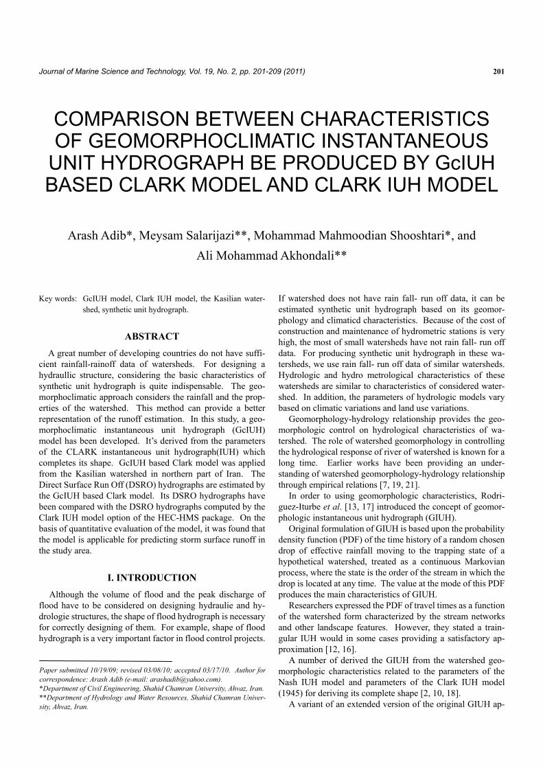
A map at an interval of 1 hr was prepared. Fig. 2 illus- trates the plot of time of travel versus cumulative area for the study area.
A. Adib et al.: Comparison between Characteristics of GIUH be Produced by Different Methods 205
010203040506070
1 2 3 4 5 6 7Time (h)
Cum
ulat
ive
area
(sq.
km)
Fig. 2. Time of travel versus cumulative area.
This information was used to formulate the no dimensional
time-area relationship of the watershed considering the nor-malized isochronal areas as the ordinates and the correspond- ing normalized times of travel as abscissas. The normalized isochronal areas are the ratios of the isochronal areas to the total watershed area. The step-wise procedure for derivation of the GcIUH-Clark model is as follows:
(i) Excess rainfall hyetograph must be computed. (ii) The peak velocity V for a given storm using the relation-
ship between peak velocity and intensity of excess-rainfall must be estimated.
(iii) Compute the time concentration using the equation:
0.2778cLtV
= .
where: tc: Time concentration (hr) L: Length of the main channel (km) (iv) Considering this tc as the largest time of travel, ordinates
of cumulative isochronal areas, corresponding to integral multiples of computational time interval, are derived us-ing the no dimensional time-area diagram. This describes the ordinates of the time-area diagram, Ii at each compu-tational time interval in the domain [0, tc];
(v) Compute the peak discharge (Qp) of GcIUH given by Eq. (15).
(vi) Compute the values of storage coefficient (R), using a non- linear optimization procedure, so that peak of the DSRO Hydrograph estimated by the Clark model (For estimation of DSRO hydrograph convolute the excess-rainfall hyeto-graph with the unit hydrograph obtained in this Step for different value of (R)) is equal to (Qp) computed in Step (v).
6. Parameter Estimation of the GcIUH-Clark Model In the gauging site of the considering watershed, the geo-
metric properties of the gauging section, the value of Man-ning’s roughness coefficient and the velocities (as a function of discharges passing through the gauging section and dif-ferent depths of flow) were measured. Kinematic wave pa-rameter for highest-order channel was estimated equal to 0.61
11 3( . )s m
−− .
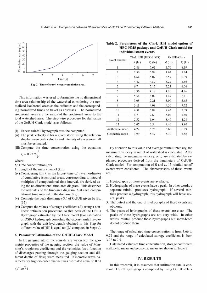
Table 2. Parameters of the Clark IUH model option of HEC-HMS package and GcIUH-Clark model for individual storm events.
Arithmetic mean 4.22 5.75 5.60 6.09Geometric mean 3.99 5.47 5.30 5.88
By attention to this value and average rainfall intensity, the
maximum velocity in outlet of watershed is calculated. After calculating the maximum velocity, R, tc are estimated by ex-plained procedure derived from the parameters of GcIUH- Clark model. For computation of R and tc, 13 rainfall-runoff events were considered. The characteristics of these events are:
1. Hyetographs of these events are available. 2. Hydrographs of these events have a peak. In other words, a
separate rainfall produces hydrograph. If several rain- falls produce a hydrograph, this hydrograph will have sev-eral peaks.
3. The outset and the end of hydrographs of these events are obvious.
4. The peaks of hydrographs of these events are clear. The peaks of these hydrographs are not very wide. In other words, rainfall produce these hydrographs but snow-broth do not produce them. The range of calculated time concentration is from 3.66 to
9.72 and the range of calculated storage coefficient is from 3.22 to 9.5.
Calculated values of time concentration, storage coefficient, arithmetic mean and geometric mean are shown in Table 2.
IV. RESULTS In this research, it is assumed that infiltration rate is con-
stant. DSRO hydrographs computed by using GcIUH-Clark
206 Journal of Marine Science and Technology, Vol. 19, No. 2 (2011)
Fig. 6. Excess rainfall hyetograph (left) and observed DSRO hydrographs and DSRO hydrographs computed by GcIUH-Clark and Clark IUH models
for event 13 (right).
A. Adib et al.: Comparison between Characteristics of GIUH be Produced by Different Methods 207
Table 3. Comparison between peak discharges of observed DSRO hydrographs and DSRO hydrographs computed by the GcIUH- Clark and Clark IUH models for 13 events.
Event number Vmax (m/s) Peak discharge of observed DSRO
hydrograph (CMS)
Peak discharge of DSRO hydro-graph computed by the Clark IUH
(HEC-HMS) (CMS)
Peak discharge of DSRO hydro-graph computed by the GcIUH-Clark (CMS)
and Clark IUH (HEC-HMS) models are compared with the observed DSRO hydrographs for four rainfall-runoff events. Error functions are evaluated for the GcIUH-Clark and Clark IUH models by using the observed DSRO hydrographs.
The parameters of Clark IUH (HEC-HMS) model were calculated by using of geometric mean of nine primary rain-fall-runoff events.
DSRO hydrographs computed by GcIUH- Clark and Clark IUH models were compared with the observed DSRO hydro-graphs as shown in Figs. 3, 4, 5 and 6 for events 10, 11, 12 and 13.
Table 3 shows comparison between peak discharges of observed DSRO hydrographs and DSRO hydrographs com-puted by GcIUH-Clark and Clark IUH models for 13 events.
The values of errors functions computed for evaluation of the DSRO hydrographs produced by GcIUH-Clark model and Clark IUH (HEC-HMS) model viz. (i) model efficiency, (ii) percentage error in peak, (iii) percentage error in time to peak, given in
2
1
2
1
( )(1 ) 100
( )
m
oi ciim
oi oi
Q QEFF
Q Q
=
=
−= − ×
−
∑
∑ (16)
where: EFF: Model efficiency (%) Qoi: ith ordinate of the observed discharge (m3/s)
oQ : Average of the ordinates of observed discharge (m3/s) Qci: Computed discharge (m3/s)
where: PETP: Percentage error in time to peak (%) Tpo: Time to peak of observed discharge (hr) Tpc: Time to peak of computed discharge (hr)
The values of error functions of GcIUH-Clark model are
shown in Fig. 7 for 13 storm events. The values of error functions of GcIUH-Clark model and
Clark IUH (HEC-HMS) model are shown in Fig. 8 for four storm events.
The range of model efficiency is from 71.37 to 89.26 per-cent for GcIUH-Clark model and it is from 5.95 to 89.45 per-cent for Clark IUH (HEC-HMS) model. Model efficiency of GcIUH-Clark model is higher than model efficiency of Clark IUH (HEC-HMS) model for 3 storm events on four storm events. Model efficiency of Clark IUH (HEC-HMS) model is very low for two storm events but model efficiency of GcIUH- Clark model is high for the total storm events.
208 Journal of Marine Science and Technology, Vol. 19, No. 2 (2011)
0102030405060708090
100
1 2 3 4 5 6 7 8 9 10 11 12 13Event number
(a)
EFF
(%)
-80-60-40-20
0204060
1 2 3 4 5 6 7 8 9 10 11 12 13
Event number(b)
PEP
(%)
-60-50-40-30-20-10
0102030
1 2 3 4 5 6 7 8 9 10 11 12 13
Event number(c)
PETP
(%)
Fig. 7. (a) Model efficiency EFF, (b) Percentage error in peak PEP, (c)
Percentage error in time to peak PETP of the GcIUH-Clark model for 13 storm events.
The range of percentage error in peak (PEP) is from 9.33 to
39.3 percent for GcIUH-Clark model and it is from -46.37 to 18.1 percent for Clark IUH (HEC-HMS) model. GcIUH- Clark model calculated the peak discharge of flood less than observed peak discharge of flood for the total storm events. Clark IUH (HEC-HMS) model calculated the peak discharge of flood less than observed peak discharge of flood in three storm events but calculated the peak discharge of flood more than observed peak discharge of flood in one storm event. Percentage error in peak (PEP) of GcIUH-Clark model is often more than percentage error in peak (PEP) of Clark IUH (HEC- HMS) model.
The range of percentage error in time to peak (PETP) is from -11.11 to 0 percent for GcIUH-Clark model and it is from 0 to 20 percent for Clark IUH (HEC-HMS) model. Under the circumstance of GcIUH-Clark model, the calculated time to peak discharge of flood equal to observed time to peak dis- charge of flood in 2 storm events but calculated time to peak discharge of flood more than observed time to peak discharge
0102030405060708090
100
1 2 3 4Event number
(a)
EFF
(%)
-60-50-40-30-20-10
01020304050
1 2 3 4
Event number(b)
PEP
(%)
-15-10-505
10152025
1 2 3 4
Event number(c)
PETP
(%)
ClarkGcIUH-Clark
ClarkGcIUH-Clark
ClarkGcIUH-Clark
Fig. 8. (a) Model efficiency EFF, (b) Percentage error in peak PEP, (c)
Percentage error in time to peak PETP of the GcIUH-Clark & Clark IUH (HEC-HMS) models for 4 storm events.
of flood in two storm events. Clark IUH (HEC-HMS) model calculated time to peak equal to observed time to peak in 1 storm event while it calculated the time to peak less than ob-served time to peak in 3 storm events. Percentage error in time to peak (PETP) of GcIUH-Clark model is often less than percentage error in time to peak (PETP) of Clark IUH (HEC- HMS) model. GcIUH-Clark model makes used of a simple rational linear relation for time concentration. Because the peak velocity is changeable for different storm events, time concentration varies in different storm events. Time concen-tration is a function of the average of rainfall intensity while storage coefficient is a function of geomorphoclimatic pa-rameters and kinematics velocity parameter. GcIUH-Clark model is independent from rainfall-runoff data. This model can simulate the shape of flood hydrograph suitability and it
A. Adib et al.: Comparison between Characteristics of GIUH be Produced by Different Methods 209
presents a suitable form of respond of watershed to storm events.
V. CONCLUSION By assuming an input of constant effective rainfall through-
out the duration of rainfall and a uniform spatial pattern of the watershed, the GcIUH-Clark model has been developed for estimation of the DSRO hydrographs for a watershed without rainfall-runoff data in northern part of Iran. In this research, the rainfall-runoff model was developed by relating the pa-rameters of Clark’s conceptual model and its geomorphocli-matic parameters and peak velocity in outlet of the watershed.
The GIUH approach provides an additional information about the effect of individual geomorphoclimatic parameters on discharge of flood. The effect of velocity on GcIUH model shows the dynamics of hydrological response of a watershed. The GcIUH-Clark model can be applied in watersheds without rainfall-runoff data. With comparison between the DSRO hydrographs estimated by GcIUH-Clark model and the ob-served DSRO hydrographs as well as with the DSRO hydro-graphs computed by Clark IUH (HEC-HMS) model, it is ob-served that the DSRO hydrographs are estimated by the GcIUH-Clark model have reasonable conformity with DSRO hydrographs estimated by the GIUH-Clark model. Even though, the GIUH-approach considers the Kasilian watershed as a watershed without rainfall-runoff data, but Clark IUH (HEC-HMS) model utilize the observed rainfall-runoff data.
The GcIUH-Clark model have an advantage over the con-ventional Clark model as it does not use historical rainfall- runoff data for DSRO estimation, and consequently, no cali-bration of the model parameters is required.
REFERENCES 1. Al-Turbak, A. S., “Geomorphoclimatic peak discharge with a physically
based infiltration component,” Journal of Hydrology, Vol. 176, No. 1-4, pp. 1-12 (1996).
2. Bhaskar, N. R., Parida, B. P., and Nayak, A. K., “Flood estimation for ungaged catchments using the GIUH,” Journal of Water Resources Planning and Management, ASCE, Vol. 123, No. 4, pp. 228-238 (1997).
3. Bras, R. L., Hydrology: An Introduction to Hydrologic Science, Addison- Wesley Publishing Company, New York, U.S.A. (1990).
4. Choi, H., Kang, J. I., Chung, H. Y., and Yoon, J. H., “Uncertainty analysis
of flash-flood system using remote sensing and a geographic information system based on GcIUH in the Yeongdeok Basin, Korea,” International Journal of Remote Sensing, Vol. 28, No. 24, pp. 5551-5565 (2007).
5. Hall, M. J., Zaki, A. F., and Shahin, M. M. A., “Regional analysis using the geomorphoclimatic instantaneous unit hydrograph,” Hydrology and Earth System Sciences, Vol. 5, No. 1, pp. 93-102 (2001).
6. Henderson, F. M., “Some properties of the unit hydrograph,” Journal of Geophysical Research, Vol. 68, pp. 4785-4793 (1963).
7. Horton, R. E., “Eros ional development of streams and their drainage basins: Hydro physical approach to quantitative morphology,” Bulletin Geological Society of America, Vol. 56, No. 3, pp. 275-370 (1945).
8. Hydrologic Engineering Center HEC, HEC-HMS—version 3.0.1, User’s Manual, U.S. Army Corps of Engineers, Washington, D.C. (2006).
9. Kumar, A. and Kumar, D., “Predicting direct runoff from hilly watershed using geomorphology and stream-order-law ratios: case study,” Journal of Hydrologic Engineering, ASCE, Vol. 13, No. 7, pp. 570-576 (2008).
10. Kumar, R., Chatterjee, C., Lohani, A. K., Kumar, S., and Singh, R.D., “Sensitivity analysis of the GIUH based Clark model for a catchment,” Water Resources Management, Vol. 16, No. 4, pp. 263-278 (2002).
11. Kurothe, R. S., Goel, N. K., and Mathur, B. S., “Derived flood frequency distribution for negatively correlated rainfall intensity and duration,” Water Resources Research, Vol. 33, No. 9, pp. 2103-2107 (1997).
12. Rinaldo, A. and Rodriguez-Iturbe, I., “Geomorphological theory of the hydrological response,” Hydrological Processes, Vol. 10, No. 6, pp. 803- 829 (1996).
13. Rodriguez-Iturbe, I., Devoto, G., and Valdes J. B., “Discharge response analysis and hydrologic similarity: The interrelation between the geo-morphologic IUH and the storm characteristics,” Water Resources Re-search, Vol. 15, No. 6, pp. 1435-1444 (1979).
14. Rodriguez-Iturbe, I., Gonzales-Sanabria, M., and Bras, R. I., “A geomor- phoclimatic theory of instantaneous unit hydrograph,” Water Resources Research, Vol. 18, No. 4, pp. 877-886 (1982).
15. Rodriguez-Iturbe, I., Gonzales-Sanabria, M., and Camano, G., “On the climatic dependence of the IUH: a rainfall-runoff theory of the Nash model and the geomorphoclimatic theory,” Water Resources Research, Vol. 18, No. 4, pp. 887-903 (1982).
16. Rodriguez-Iturbe, I. and Rinaldo, A., Fractal River Basins: Chance and self-organization, Cambridge University Press, New York. (1997).
17. Rodriguez-Iturbe, I. and Valdes, J. B., “The geomorphic structure of hydrologic response,” Water Resources Research, Vol. 15, No. 6, pp. 1409- 1420 (1979).
18. Sahoo, B., Chatterjee, C., Raghuwanshi, N. S., and Singh, R., “Flood estimation by GIUH-based Clark and Nash models,” Journal of Hydro-logic Engineering, ASCE, Vol. 11, No. 6, pp. 515-525 (2006).
19. Snyder, F. F., “Synthetic unit graphs,” Transactions of American Geo-physics Union, 19th Annual Meeting, Part 2 (1938).
20. Strahler, A. N., “Quantitative slope analysis,” Bulletin Geological Society of America, Vol. 67, No. 5, pp. 571-596 (1956).
21. Taylor, A. B. and Schwartz, H. E., “Unit-hydrograph lag and peak flow related to basin characteristics,” Transactions of American Geophysics Union, Vol. 33, pp. 235-246 (1952).