PNNL-20388

Prepared for the U.S. Army Corps of Engineers, Portland District Under an Interagency Agreement with the U.S. Department of Energy Contract DE-AC05-76RL01830

Compliance Monitoring of Underwater Blasting for Rock Removal at Warrior Point, Columbia River Channel Improvement Project, 2009/2010 COMPLETION REPORT TJ Carlson GE Johnson CM Woodley JR Skalski AG Seaburg May 2011

PNNL-20388

Compliance Monitoring of Underwater Blasting for Rock Removal at Warrior Point, Columbia River Channel Improvement Project, 2009/2010 COMPLETION REPORT TJ Carlson1 GE Johnson1 CM Woodley1 JR Skalski 2 AG Seaburg2 May 2011 Prepared for the U.S. Army Corps of Engineers, Portland District Under a Government Order with the U.S. Department of Energy Contract DE-AC05-76RL01830 Prepared by: Pacific Northwest National Laboratory, Marine Sciences Laboratory University of Washington, Columbia Basin Research 1 Pacific Northwest National Laboratory, Richland, Washington 2 University of Washington, Seattle, Washington.

iii

Summary

The U.S. Army Corps of Engineers, Portland District (USACE) conducted the 20-year Columbia River Channel Improvement Project (CRCIP) to deepen the navigation channel between Portland, Oregon and the Pacific Ocean to allow transit of fully loaded Panamax ships (100 ft wide, 600 to 700 ft long, and draft 45 to 50 ft). Blasting was necessary in a 1-mile stretch of the total ~100 miles of navigation channel to reach a depth of at least 44 ft in the Columbia River navigation channel. In the vicinity of Warrior Point, between river miles (RM) 87 and 88 near St. Helens, Oregon, the USACE used underwater blasting and dredging to remove about 300,000 yd3 of a basalt rock formation. Blast events consisted of arrays of single charges with up to 78 charges per event. Usually there were one or two blast events per day between initiation of test blasting on November 1, 2009, and completion of production blasting on February 5, 2010. Over the course of the work, there were a total of 99 blasting events.

The purpose of this report is to document methods and results of the compliance monitoring study for the blasting project at Warrior Point in the Columbia River. The permit for blasting operations granted by regulatory agencies required the USACE to monitor impacts on aquatic animal species, including marine mammals, diving birds, sturgeon, and salmonids. The USACE developed an approved monitoring plan and the Pacific Northwest National Laboratory (PNNL), in collaboration with the University of Washington and under contract to the USACE, performed compliance monitoring and reported results daily for all 99 blasting events. The USACE, in coordination with the regulatory agencies, used compliance monitoring data in near real-time to evaluate whether blasting operations were meeting standards set forth in the permit, most importantly, presence of marine mammals in the study area and take of salmonids as a result of blasting operations.

The detailed objectives of compliance monitoring were to accomplish the following:

• Prior to a blast

– Survey a region, called the safety zone, that extends beyond the impact area 2,000 ft upstream and 2,000 ft downstream from the blasting location for the presence of marine mammals and protected birds and report their location to responsible parties prior to blasting.

– Within the safety zone, pay particular attention for marine mammals in a 500-ft marine mammal monitoring zone around the blasting location.

– Approximate the number of adult sturgeon likely to occur within the impact area during a blast.

– Estimate the flux of adult- and juvenile-size salmon listed as endangered under the Endangered Species Act (ESA) into the impact area prior to blasting.

• During a blast

– Document the number of marine mammals in the safety zone and the 500-ft marine mammal monitoring zone at the blast site.

– Measure blast impulse pressures.

– Determine response of juvenile salmonids exposed to blast impulse pressures.

iv

• After a blast

– Survey the impact area and enumerate the number of dead ESA-listed fish, recover as many bodies as possible, and perform necropsies to determine cause of death on a subset of, or all, recovered bodies, depending on the number recovered.

– Prepare a daily report of compliance monitoring results.

– Estimate the take of adult- and juvenile-size listed salmon.

Over the duration of blasting, the distribution of adult salmon within a region surrounding blast events defined by the likelihood of mortality of adult salmon to blast pressure was determined using active acoustics. The probable take (mortality) of adult salmon through the monitored region was estimated using peak blast pressure and blast impulse observed by the blasting contractor and a likelihood model for the probability of mortality obtained by reanalysis of published data. Over the course of blasting the take of adult salmon was essentially zero based on the low number of adult salmon migrants and the very low level of blast pressures. Observed absolute peak blast pressure ranged from 4.78 psi (33 kPa) to 84 psi (576 kPa) with a mean and median of 22 and 19 psi (153 and 133 kPa), respectively. Obsergved blast pressures and impulses were low compared to in-water blast pressures for the equivalent weights of explosive because the charges were located in massive rock and were further confined by 10 feet of pea gravel (stemming). In addition, the charges within an array were detonated with time delays between the charges.

The blasting monitoring plan required estimation of the likely take of juvenile chum salmon following emergence of juveniles from redds. The strategy for estimating take of juvenile chum followed that for adult salmon with active acoustic monitoring to observe the flux of juveniles into the impact area with take estimated using observed blast pressures and a mortality likelihood model. The main difference was no data were available for juvenile salmon to derive a mortality likelihood model. To fill this information gap we conducted a study of the response of juvenile Chinook salmon (126 mm fork length [FL] ± 25 mm) and juvenile rainbow trout (68 mm FL ± 4 mm) to blast pressure. Unique cages were designed that were stable in the high velocity flow of the river. The design of the cages also provided access by the juvenile fish confined within the cage to an air pocket. Access to free air provided test fish the opportunity to acclimate by attaining neutral buoyancy at the exposure static pressure. The exposure peak blast pressures for test fish were low compared to blast pressures reported in the literature and ranged from 4 to 24 psi (28 kPa to 164 kPa). Samples of exposed and control test fish were examined externally and by necropsy immediately following exposure and also at 24 and 48 hours post exposure. An analysis model, Fish Index of Trauma (FIT), was developed to describe the response of test fish to blast pressure exposures. A model was derived with blast maximum positive pressure as the predictor variable and the FIT model metric RSWI (Response Severity Weighted Index) as the predicted variable that explained 56% of the variability observed in fish response at exposure to very low blast pressures. Analysis of fish condition at 24 and 48 hours post exposure showed that juvenile Chinook salmon and rainbow trout have the potential to recover from some blast exposure injuries while injury severity increased with time for other blast injuries. During the holding period, no mortalities resulting from blast injuries were observed for test fish.

The monitoring results showed harbor seals were present in the safety zone, 2,000 ft upstream and 2,000 ft downstream of the blast site, throughout the 3-month study period. During 93 of the 99 blasts, at least one marine mammal was observed in the safety zone during the designated monitoring period. We

v

also observed two California sea lions in the safety zone. Four marine mammals were present in the safety zone at blasting time. Most importantly, however, no marine mammals were observed within the 500-ft marine mammal monitoring zone at blasting time for any of the blasts. During post-blast surveys, we recovered three dead sturgeon. We did not observe any dead marine mammals or salmon after the blasts.

In summary, impacts on marine mammals were not observed and the cumulative take of juvenile and adult salmon was essentially zero. Blasting occurred after most of the adult salmon migration had passed the study area and was completed before juvenile chum salmon arrived. The dose-exposure-response approach to estimating take provided an unobtrusive, science-based method that allowed near real-time reporting of results as required by the regulators. Conducting the project during the November–February timeframe when biological activity in the river is minimal helped the project comply with federal and state requirements to not adversely affect marine mammals and fishes. The compliance monitoring data confirmed that USACE blasting operations met the standards set forth in the permit granted by the regulatory agencies.

vii

Preface

This study was conducted by researchers at the Pacific Northwest National Laboratory (PNNL) and the University of Washington (UW) for the U.S. Army Corps of Engineers, Portland District (USACE). The PNNL and UW project managers were Drs. Thomas J. Carlson and John R. Skalski, respectively. The USACE technical leads were Blaine Ebberts (fisheries biology) and John Cannon (construction engineering). The USACE program manager was Laura Hicks. The data are archived at the Marine Sciences Laboratory in Sequim, Washington. For more information about the study, contact Carlson (503 417 7562) or Hicks (503 808 4703).

The original scope of work for reporting study results included only daily reports during the blasting period. The USACE subsequently requested this completion report to document methods and findings of this unique monitoring effort for others to learn from and apply in any future work of this kind. Two of the report’s main chapters—estimation of take and fish response—are intended to be submitted for publication in the peer-reviewed literature. As such, the chapters were written as stand-alone documents for the most part.

Recommended citation: Carlson TJ, GE Johnson, CM Woodley, JR Skalski, AG Seaburg. 2011. Compliance Monitoring of Underwater Blasting for Rock Removal at Warrior Point, Columbia River Channel Improvement Project, 2009/2010. PNNL-20388, prepared by Pacific Northwest National Laboratory, Richland, Washington for the U.S. Army Corps of Engineers, Portland District, Portland, Oregon.

ix

Acknowledgments

We gratefully acknowledge the contributions to the compliance monitoring effort from the following people.

• USACE – J. Cannon, B. Ebberts, L. Hicks, K. Larson

• McAmis – Scott Vandegrift

• PNNL – staff devoted almost full-time to the study:

Carpenter, S Carter, K Faber, D Fischer, E Gaulke, G Hall, K Karls, R Knox, K Monter, T Vavrinec, J Solcz, A Mueller, R Phillips, N

• PNNL – staff played a significant role in execution of the study:

Anderson, C Bryson, A Carter, J Cushing, A Dirkes, G Fortman, T Gruendell, B Hughes, J Hughes, J Kauffman, M Lavender, K Southard, S Smith, J Wilberding, M Deng, Z Weiland, M

• PNNL – other staff also helped make the study a success:

Anderson, M Duberstein, C Gay, M Gingerich, A Myers, J O’Reilly, J Walker, R Zimmerman, S

xi

Acronyms and Abbreviations

ADCP acoustic Doppler current profiler ANOCOV analyses of covariance ANOVA analyses of variance ATU accumulate temperature unit BMPP blast maximum positive pressure cfs cubic (foot)feet per second cm centimeter(s) CRCIP Columbia River Channel Improvement Project dB decibel(s) DIDSON Dual-Frequency Identification Sonar DVD digital video disc ESA Endangered Species Act FIT Fish Index of Trauma FL fork length FRSWI Fish Response Severity Weighted Index ft foot(feet) ft2 square foot(feet) ft-sec (foot)feet per second (also ft/sec) g gram(s) gal gallon(s) GI gastrointestinal GPS global positioning system h hour(s) hp horsepower Hz hertz in. inch(es) ISS Injury Severity Score kHz kilohertz L liter lb pound(s) m meter(s) m3 cubic meter(s) mg milligram(s) min minute(s) mm millimeter(s) msec millisecond(s)

xii

NISS New Injury Severity Score NMFS National Marine Fisheries Service Pa pascal(s) PAS Precision Acoustic Systems, Inc. PNNL Pacific Northwest National Laboratory psi pounds per square inch RM river mile RMS root-mean-square RTS Revised Trauma Score SPOC single point-of-contact USACE U.S. Army Corps of Engineers USGS U.S. Geological Survey UW University of Washington yd3 cubic yards WDFW Washington Department of Fish and Wildlife Wt weight

xiii

Contents

Summary ............................................................................................................................................... iii Preface .................................................................................................................................................. vii Acknowledgments ................................................................................................................................. ix Acronyms and Abbreviations ............................................................................................................... xi 1.0 Introduction .................................................................................................................................. 1.1

1.1 The Study Area .................................................................................................................... 1.1 1.2 Study Overview .................................................................................................................... 1.2 1.3 Report Contents and Organization ....................................................................................... 1.3

2.0 Compliance Monitoring ................................................................................................................ 2.1 2.1 Objectives ............................................................................................................................. 2.2 2.2 Methods ................................................................................................................................ 2.2

2.2.1 Equipment and Sampling Design .............................................................................. 2.3 2.2.2 Sequence of Monitoring Events for the Typical Blast .............................................. 2.4 2.2.3 Marine Mammals ...................................................................................................... 2.5 2.2.4 Diving Birds .............................................................................................................. 2.5 2.2.5 Sturgeon .................................................................................................................... 2.5 2.2.6 Daily Reports ............................................................................................................. 2.6

2.3 Results .................................................................................................................................. 2.6 2.3.1 River Conditions ....................................................................................................... 2.7 2.3.2 Blasting Operations ................................................................................................... 2.7 2.3.3 Observations of Marine Mammals and Diving Birds ................................................ 2.8 2.3.4 Compliance................................................................................................................ 2.8

2.4 Summary and Conclusion .................................................................................................... 2.9 3.0 Estimation of Take ........................................................................................................................ 3.1

3.1 Methodology ........................................................................................................................ 3.2 3.1.1 Dose ........................................................................................................................... 3.2 3.1.2 Exposure .................................................................................................................... 3.3 3.1.3 Response ................................................................................................................... 3.5 3.1.4 Take ........................................................................................................................... 3.7

3.2 Results .................................................................................................................................. 3.8 3.3 Summary and Conclusion .................................................................................................... 3.12

4.0 Response of Caged Juvenile Salmonids to High-Energy Impulsive Sound ................................ 4.1 4.1 Methods and Materials ......................................................................................................... 4.2

4.1.1 Fish Acquisition ........................................................................................................ 4.2 4.1.2 Fish Housing ............................................................................................................. 4.2 4.1.3 Caged Fish Deployment ............................................................................................ 4.3

xiv

4.1.4 Sham Fish .................................................................................................................. 4.6 4.1.5 Pressure Recording and Analysis .............................................................................. 4.6 4.1.6 Necropsy ................................................................................................................... 4.6 4.1.7 Data Adjustments ...................................................................................................... 4.7 4.1.8 Injury Descriptions .................................................................................................... 4.8 4.1.9 Statistical Methods .................................................................................................... 4.10

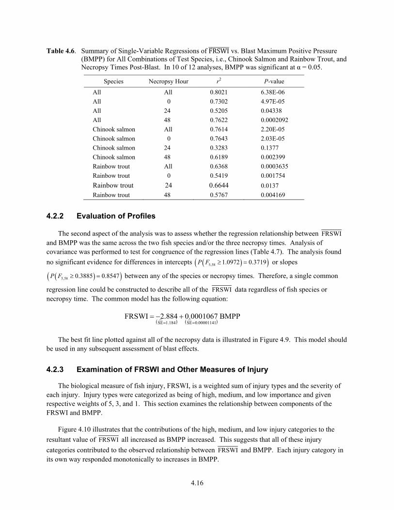
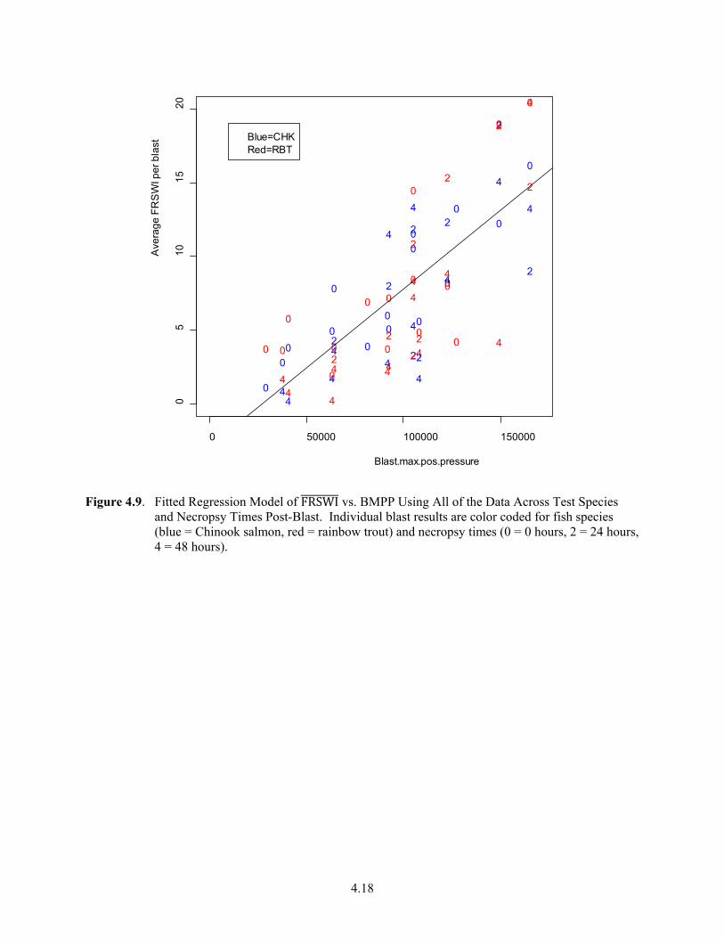
4.2 Results .................................................................................................................................. 4.11 4.2.1 Model Selection ......................................................................................................... 4.11 4.2.2 Evaluation of Profiles ................................................................................................ 4.16 4.2.3 Examination of FRSWI and Other Measures of Injury ............................................. 4.16

4.3 Summary and Conclusion .................................................................................................... 4.21 5.0 Literature Cited ............................................................................................................................. 5.1 Appendix A – Marine Mammal Monitoring Protocol .......................................................................... A.1 Appendix B – Data Protocols ............................................................................................................... B.1 Appendix C – Boat Operations ............................................................................................................. C.1 Appendix D – Hydroacoustic System Specifications ........................................................................... D.1 Appendix E – Monitoring Events ......................................................................................................... E.1 Appendix F – Fish Injury References: A Photographic Guide ............................................................ F.1

xv

Figures

1.1 Project Site on the Columbia River Near Warrior Point near St. Helens, Oregon ...................... 1.2 1.2 Depiction of Bathymetry at the Project Site ................................................................................ 1.2 2.1 Arrangement of Monitoring Boats Relative to the Blast Array .................................................. 2.4 2.2 Approximate Mobile Track Lines for Sturgeon Surveys ............................................................ 2.6 2.3 Mean Daily Discharge at Columbia River Mile 54 ..................................................................... 2.7 2.4 Mean Daily Gage Height at Columbia River Mile 54 ................................................................. 2.7 3.1 Schematic of the Dose-Exposure-Response Approach for Take Estimation .............................. 3.2 3.2 Schematic Longitudinal Cross-Section of the Deployment of Transducers to Sample Fish

Flux ............................................................................................................................................. 3.4 3.3 Logistic Relationship Between Blast Impulse and Probability of Mortality for Adult

Salmonids .................................................................................................................................... 3.7 3.4 Absolute Value of Maximum Pressure ....................................................................................... 3.9 3.5 The Sound Wave Form Observed for a Single Blast Event ........................................................ 3.9 3.6 Fish Flux During Compliance Monitoring .................................................................................. 3.10 3.7 Counts of Adult Salmon at Bonneville Dam and Adult Chum Salmon at the Spawning Area

Near Ives Island Just Downstream of Bonneville Dam .............................................................. 3.10 3.8 Take by Blast During Compliance Monitoring ........................................................................... 3.11 3.9 Cumulative Take During Compliance Monitoring ..................................................................... 3.11 3.10 Accumulated Temperature Units and Estimated Emergence Timing for Chum Salmon at

Ives Island ................................................................................................................................... 3.12 4.1 Holding Totes Used in This Study for Pre- and Post-Exposure Fish .......................................... 4.3 4.2 Wedge Shape Blast Exposure Cages ........................................................................................... 4.4 4.3 A Photograph of the Barge with the Sensor Recording Box and Air Pump Secured Within

the White Cooler ......................................................................................................................... 4.4 4.4 A View of the Barge in Line with the Drilling of the Holes for Blasting ................................... 4.5 4.5 An Example of a Typical Production Blast Plan Report ............................................................. 4.5

4.6 Plots of FRSWI vs. Blast Maximum Positive Pressure for Chinook Salmon and Rainbow Trout Combined with Necropsy Results at 0 Hours, 24 Hours, and 48 Hours Post-Blast .......... 4.13

4.7 Plots of FRSWI vs. Blast Maximum Positive Pressure for Chinook Salmon for Necropsy Results at 0 hours, 24 hours, and 48 Hours Post-Blast ............................................................... 4.14

4.8 Plots of FRSWI vs. Blast Maximum Positive Pressure for Rainbow Trout for Necropsy Results at 0 Hours, 24 Hours, and 48 Hours Post-Blast .............................................................. 4.15

4.9 Fitted Regression Model of FRSWI vs. BMPP Using All of the Data Across Test Species and Necropsy Times Post-Blast .................................................................................................. 4.18

4.10 Scatter Plots and Fitted Linear Relationships Between BMPP and Component Scores for FRSWI in the High Injury Category, Medium Injury Category, and Low Injury Category ....... 4.19

4.11 Three-Dimensional Plot Illustrating the Frequency at Which Fish Were Observed Having Different Numbers of Injuries as BMPP Increased ..................................................................... 4.20

4.12 Scatter Plot of Mean Number of Injuries per Fish in a Test Group vs. BMPP and Fitted Linear Regression Line ............................................................................................................... 4.20

xvi

Tables 2.1 Excerpts from the Biological Opinion for the Columbia River Channel Improvement

Project ......................................................................................................................................... 2.1 2.2 Monitoring Equipment and Deployment Techniques ................................................................. 2.3 2.3 Sampling Design – Monitoring Locations and Frequencies ....................................................... 2.3 2.4 PNNL Boats Used for Compliance Monitoring .......................................................................... 2.3 2.5 Idealized Sequence of Monitoring Activities .............................................................................. 2.4 2.6 Example Daily Report ................................................................................................................. 2.6 2.7 Blasting and Monitoring Statistics .............................................................................................. 2.8 2.8 Summary of Compliance Monitoring Results ............................................................................. 2.8 3.1 Probit Equations for the Relationship Between Impulsive Sound Pressure and Fish

Response .................................................................................................................................... 3.5 3.2 Logit Values for the Probabilities of Mortality for the Range of Impulses of Interest ............... 3.6 3.3 Linear Regression Used to Estimate the Logistic Function Parameters ...................................... 3.6 4.1 Fish Size Range ........................................................................................................................... 4.2 4.2 An Abbreviated List of Barotrauma and Pre-Existing Injuries ................................................... 4.7

4.3 Results of Sequential Stepwise Regression of FRSWI Against Alternative Measures of Blast Strength Using Both Fish Species and All Necropsy Times ............................................. 4.11

4.4 Results of Sequential Stepwise Regression of FRSWI Against Alternative Measures of Blast Strength for Chinook Salmon and All Necropsy Times .................................................... 4.12

4.5 Results of Sequential Stepwise Regression of FRSWI Against Alternative Measures of Blast Strength for Rainbow Trout and All Necropsy Times ....................................................... 4.12

4.6 Summary of Single-Variable Regressions of FRSWI vs. Blast Maximum Positive Pressure for All Combinations of Test Species, i.e., Chinook Salmon and Rainbow Trout, and Necropsy Times Post-Blast ......................................................................................................... 4.16

4.7 Analyses of Covariance for FRSWI vs. BMPP ........................................................................... 4.17

1.1

1.0 Introduction

The U.S. Army Corps of Engineers, Portland District (USACE) conducted the 20-year Columbia River Channel Improvement Project (CRCIP) to deepen the navigation channel between Portland, Oregon, and the Pacific Ocean to allow transit of fully loaded Panamax ships (100 ft wide, 600 to 700 ft long, and draft 45 to 50 ft). In the vicinity of Warrior Point, between river miles (RM) 87 and 88 near St. Helens, Oregon, the USACE conducted underwater blasting and dredging to remove 300,000 yd3 of a basalt rock formation to reach a depth of 44 ft in the Columbia River navigation channel. Blasting was necessary in a 1-mile stretch of the total ~100 miles of navigation channel.

The purpose of this report is to document methods and results of the compliance monitoring study for the blasting project at Warrior Point in the Columbia River. The permit for blasting operations granted by regulatory agencies required the USACE to monitor impacts on aquatic animal species, including marine mammals, diving birds, sturgeon, and salmonids. The USACE developed an approved monitoring plan and the Pacific Northwest National Laboratory (PNNL), in collaboration with the University of Washington and under contract to the USACE, performed compliance monitoring and reported results daily for all 99 blasting events conducted from November 1, 2009 through February 5, 2010. The USACE, in coordination with the regulatory agencies, used compliance monitoring data in near real-time to evaluate whether blasting operations were meeting standards set forth in the permit, most importantly, presence of marine mammals in the study area and take of salmonids as a results of blasting operations—no marine mammals inside the 500-ft (radius) marine mammal monitoring zone at blast time and no more than 10 adult and 50 juvenile listed salmonids taken for all blast events combined (NMFS 2002).

This report has the following objectives:

1. Describe the methods and results of compliance monitoring for the blasting project.

2. Document the methods and results for estimation of take of salmonids.

3. Determine the relationship between high-energy impulsive sound and response of caged juvenile salmonids.

1.1 The Study Area

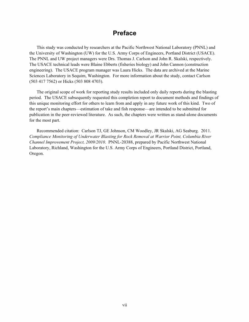
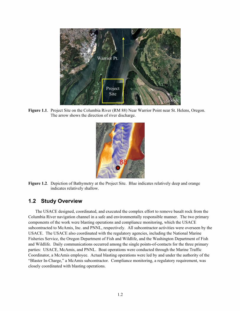
The study area in which the monitoring was conducted is located between RM 87 and 88 on the Columbia River near Warrior Point (Figure 1.1). The area is upstream of the confluence of the Columbia River and Lake River on the Washington side. The area is bounded by Sauvie Island on the Oregon shore and Bachelor Island on the Washington shore. The Columbia River flows north through this area and is tidally influenced. The Columbia River basalt outcropping that was removed by underwater blasting protruded from the Oregon side of the river (Figure 1.2).

1.2

Figure 1.1. Project Site on the Columbia River (RM 88) Near Warrior Point near St. Helens, Oregon.

The arrow shows the direction of river discharge.

Figure 1.2. Depiction of Bathymetry at the Project Site. Blue indicates relatively deep and orange

indicates relatively shallow.

1.2 Study Overview

The USACE designed, coordinated, and executed the complex effort to remove basalt rock from the Columbia River navigation channel in a safe and environmentally responsible manner. The two primary components of the work were blasting operations and compliance monitoring, which the USACE subcontracted to McAmis, Inc. and PNNL, respectively. All subcontractor activities were overseen by the USACE. The USACE also coordinated with the regulatory agencies, including the National Marine Fisheries Service, the Oregon Department of Fish and Wildlife, and the Washington Department of Fish and Wildlife. Daily communications occurred among the single points-of-contacts for the three primary parties: USACE, McAmis, and PNNL. Boat operations were conducted through the Marine Traffic Coordinator, a McAmis employee. Actual blasting operations were led by and under the authority of the “Blaster In-Charge,” a McAmis subcontractor. Compliance monitoring, a regulatory requirement, was closely coordinated with blasting operations.

Project Site

Warrior Pt.

1.3

1.3 Report Contents and Organization

The ensuing chapters of this report describe the objectives, methods, and results of routine compliance monitoring for marine mammals, diving birds, sturgeon, and associated post-blasting mortalities (Chapter 2.0). Chapter 3.0 documents the methods developed to estimate the take of salmonids listed under the Endangered Species Act and the take results for the compliance monitoring study. Chapter 4.0 describes the response of caged juvenile salmonids to high-energy impulsive sound during blasting. Citations are listed in Chapter 5.0. Appendixes A through E provide supplemental technical details about the marine mammal monitoring protocol (A), data protocols (B), boat operations (C), hydroacoustic system specifications (D), monitoring events (E), and a photographic reference guide to fish injuries (F).

2.1

2.0 Compliance Monitoring

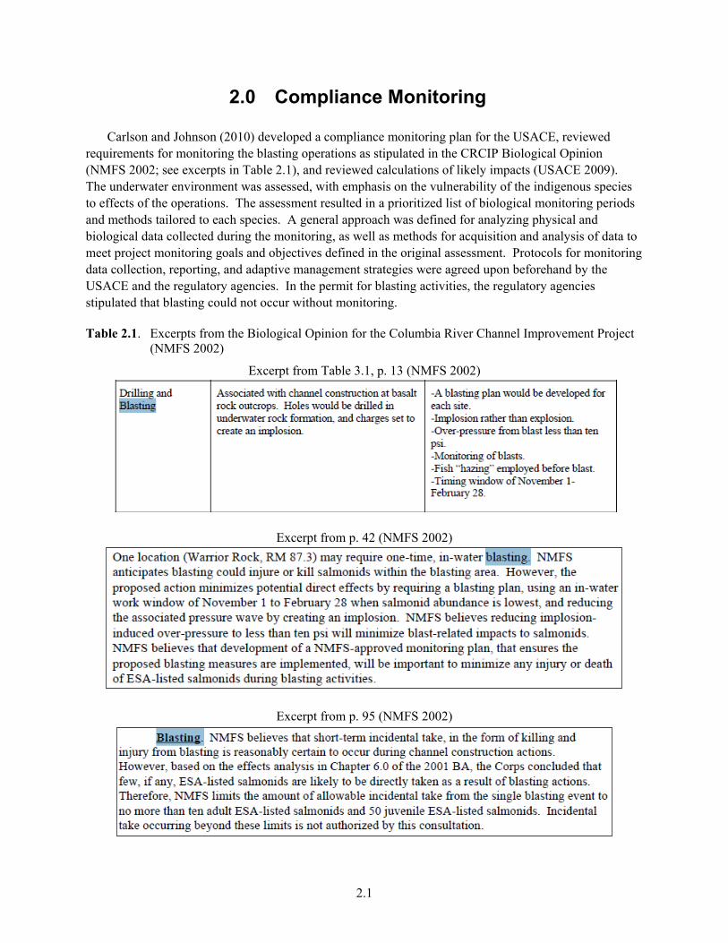
Carlson and Johnson (2010) developed a compliance monitoring plan for the USACE, reviewed requirements for monitoring the blasting operations as stipulated in the CRCIP Biological Opinion (NMFS 2002; see excerpts in Table 2.1), and reviewed calculations of likely impacts (USACE 2009). The underwater environment was assessed, with emphasis on the vulnerability of the indigenous species to effects of the operations. The assessment resulted in a prioritized list of biological monitoring periods and methods tailored to each species. A general approach was defined for analyzing physical and biological data collected during the monitoring, as well as methods for acquisition and analysis of data to meet project monitoring goals and objectives defined in the original assessment. Protocols for monitoring data collection, reporting, and adaptive management strategies were agreed upon beforehand by the USACE and the regulatory agencies. In the permit for blasting activities, the regulatory agencies stipulated that blasting could not occur without monitoring.

Table 2.1. Excerpts from the Biological Opinion for the Columbia River Channel Improvement Project (NMFS 2002)

Excerpt from Table 3.1, p. 13 (NMFS 2002)

Excerpt from p. 42 (NMFS 2002)

Excerpt from p. 95 (NMFS 2002)

2.2

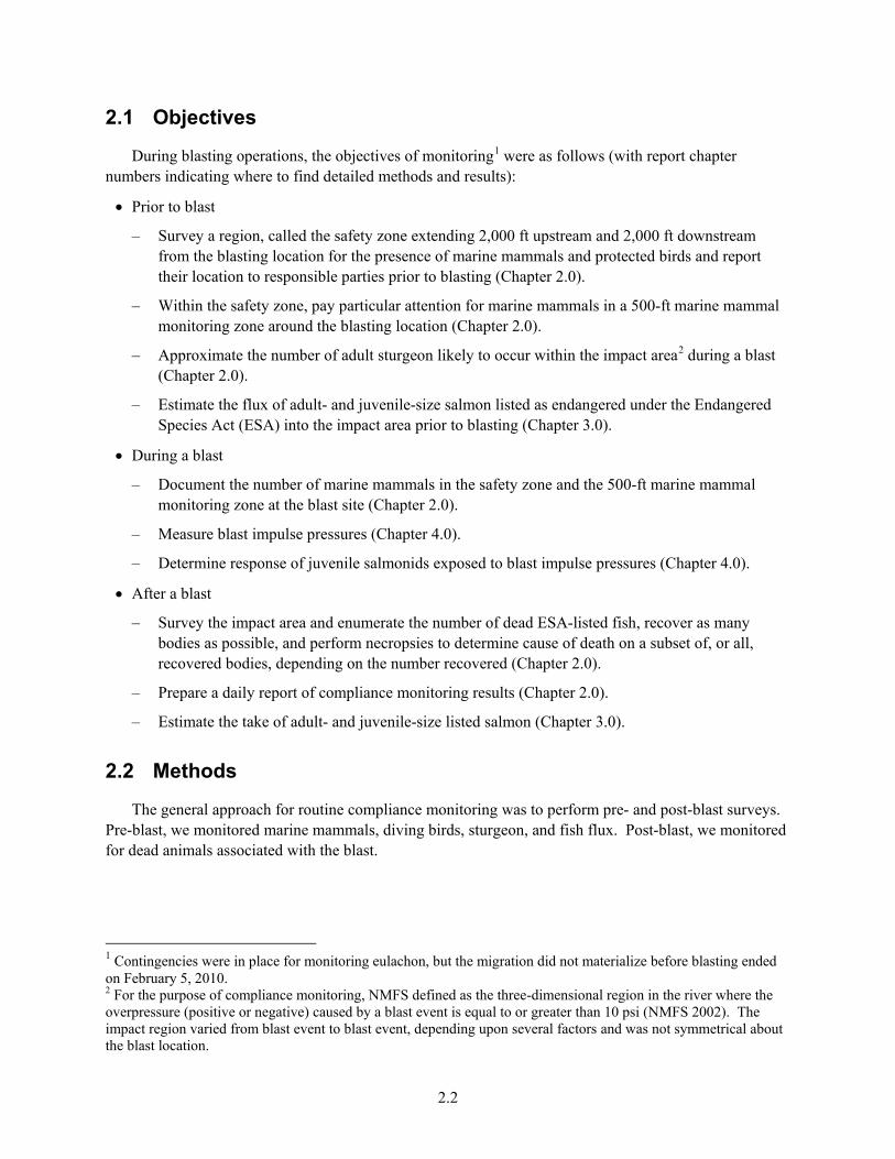
2.1 Objectives

During blasting operations, the objectives of monitoring1 were as follows (with report chapter numbers indicating where to find detailed methods and results):

• Prior to blast

– Survey a region, called the safety zone extending 2,000 ft upstream and 2,000 ft downstream from the blasting location for the presence of marine mammals and protected birds and report their location to responsible parties prior to blasting (Chapter 2.0).

– Within the safety zone, pay particular attention for marine mammals in a 500-ft marine mammal monitoring zone around the blasting location (Chapter 2.0).

– Approximate the number of adult sturgeon likely to occur within the impact area2 during a blast (Chapter 2.0).

– Estimate the flux of adult- and juvenile-size salmon listed as endangered under the Endangered Species Act (ESA) into the impact area prior to blasting (Chapter 3.0).

• During a blast

– Document the number of marine mammals in the safety zone and the 500-ft marine mammal monitoring zone at the blast site (Chapter 2.0).

– Measure blast impulse pressures (Chapter 4.0).

– Determine response of juvenile salmonids exposed to blast impulse pressures (Chapter 4.0).

• After a blast

– Survey the impact area and enumerate the number of dead ESA-listed fish, recover as many bodies as possible, and perform necropsies to determine cause of death on a subset of, or all, recovered bodies, depending on the number recovered (Chapter 2.0).

– Prepare a daily report of compliance monitoring results (Chapter 2.0).

– Estimate the take of adult- and juvenile-size listed salmon (Chapter 3.0).

2.2 Methods

The general approach for routine compliance monitoring was to perform pre- and post-blast surveys. Pre-blast, we monitored marine mammals, diving birds, sturgeon, and fish flux. Post-blast, we monitored for dead animals associated with the blast.

1 Contingencies were in place for monitoring eulachon, but the migration did not materialize before blasting ended on February 5, 2010. 2 For the purpose of compliance monitoring, NMFS defined as the three-dimensional region in the river where the overpressure (positive or negative) caused by a blast event is equal to or greater than 10 psi (NMFS 2002). The impact region varied from blast event to blast event, depending upon several factors and was not symmetrical about the blast location.

2.3

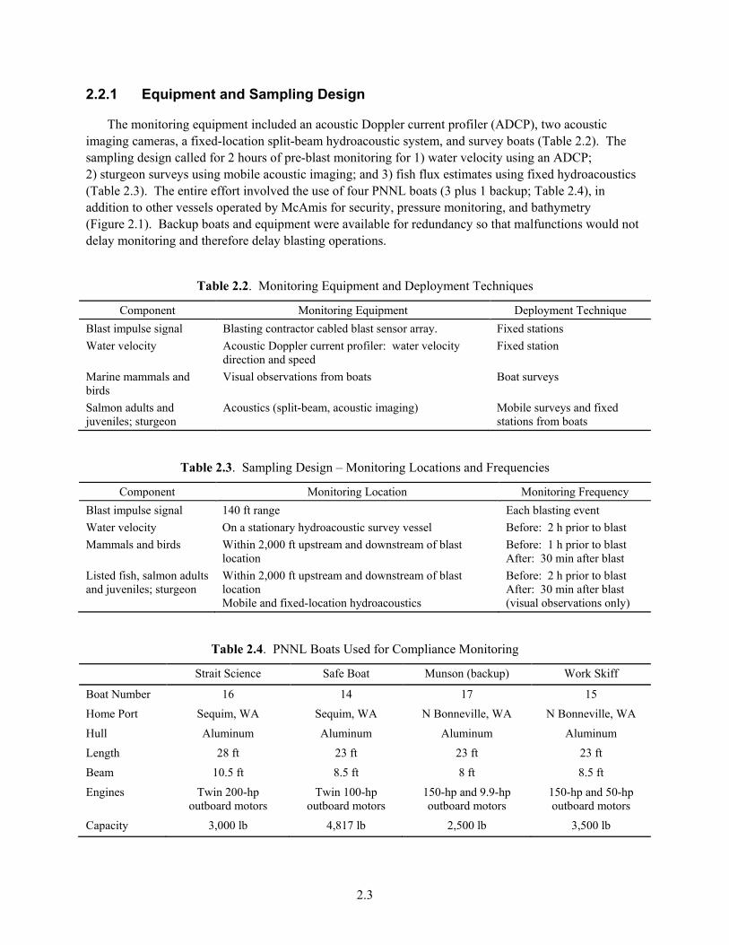
2.2.1 Equipment and Sampling Design

The monitoring equipment included an acoustic Doppler current profiler (ADCP), two acoustic imaging cameras, a fixed-location split-beam hydroacoustic system, and survey boats (Table 2.2). The sampling design called for 2 hours of pre-blast monitoring for 1) water velocity using an ADCP; 2) sturgeon surveys using mobile acoustic imaging; and 3) fish flux estimates using fixed hydroacoustics (Table 2.3). The entire effort involved the use of four PNNL boats (3 plus 1 backup; Table 2.4), in addition to other vessels operated by McAmis for security, pressure monitoring, and bathymetry (Figure 2.1). Backup boats and equipment were available for redundancy so that malfunctions would not delay monitoring and therefore delay blasting operations.

Table 2.2. Monitoring Equipment and Deployment Techniques

Component Monitoring Equipment Deployment Technique Blast impulse signal Blasting contractor cabled blast sensor array. Fixed stations Water velocity Acoustic Doppler current profiler: water velocity

direction and speed Fixed station

Marine mammals and birds

Visual observations from boats Boat surveys

Salmon adults and juveniles; sturgeon

Acoustics (split-beam, acoustic imaging) Mobile surveys and fixed stations from boats

Table 2.3. Sampling Design – Monitoring Locations and Frequencies

Component Monitoring Location Monitoring Frequency Blast impulse signal 140 ft range Each blasting event Water velocity On a stationary hydroacoustic survey vessel Before: 2 h prior to blast Mammals and birds Within 2,000 ft upstream and downstream of blast

location Before: 1 h prior to blast After: 30 min after blast

Listed fish, salmon adults and juveniles; sturgeon

Within 2,000 ft upstream and downstream of blast location Mobile and fixed-location hydroacoustics

Before: 2 h prior to blast After: 30 min after blast (visual observations only)

Table 2.4. PNNL Boats Used for Compliance Monitoring

Strait Science Safe Boat Munson (backup) Work Skiff

Boat Number 16 14 17 15 Home Port Sequim, WA Sequim, WA N Bonneville, WA N Bonneville, WA Hull Aluminum Aluminum Aluminum Aluminum Length 28 ft 23 ft 23 ft 23 ft Beam 10.5 ft 8.5 ft 8 ft 8.5 ft Engines Twin 200-hp

outboard motors Twin 100-hp

outboard motors 150-hp and 9.9-hp outboard motors

150-hp and 50-hp outboard motors

Capacity 3,000 lb 4,817 lb 2,500 lb 3,500 lb

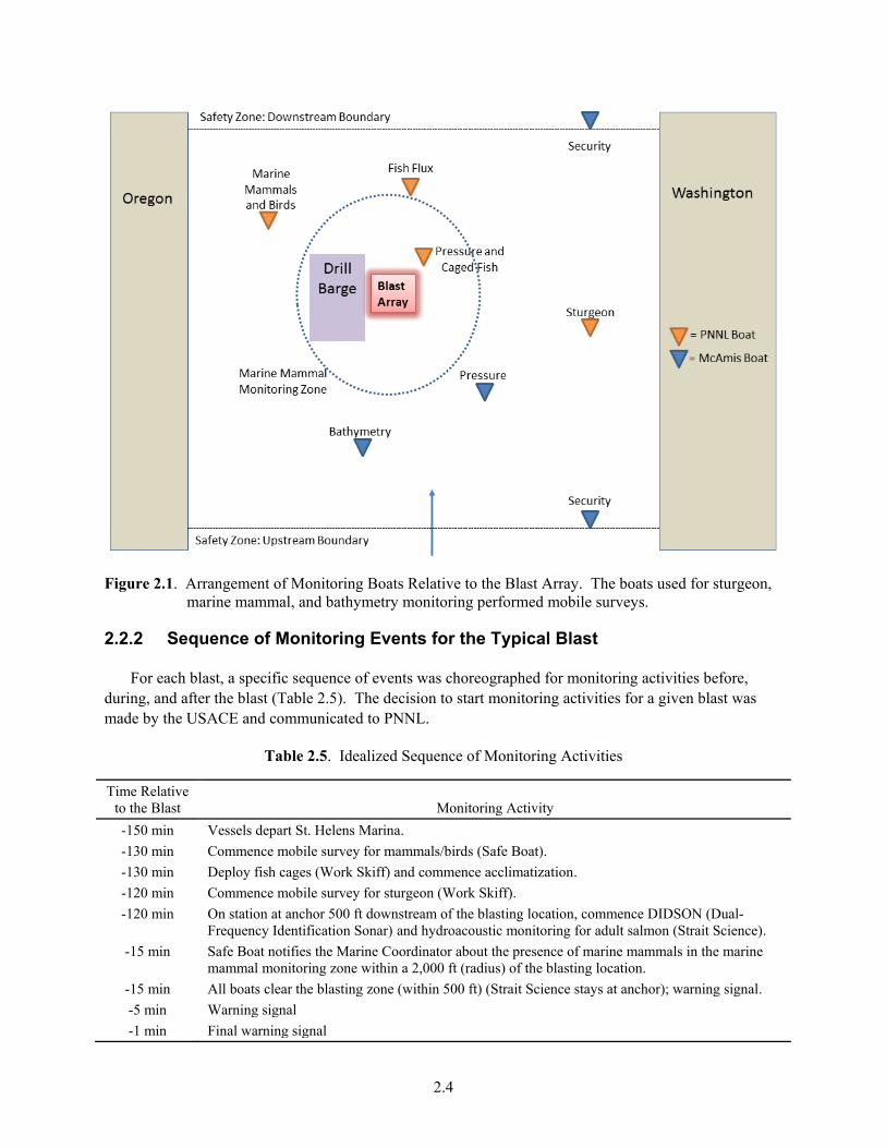
2.4

Figure 2.1. Arrangement of Monitoring Boats Relative to the Blast Array. The boats used for sturgeon, marine mammal, and bathymetry monitoring performed mobile surveys.

2.2.2 Sequence of Monitoring Events for the Typical Blast

For each blast, a specific sequence of events was choreographed for monitoring activities before, during, and after the blast (Table 2.5). The decision to start monitoring activities for a given blast was made by the USACE and communicated to PNNL.

Table 2.5. Idealized Sequence of Monitoring Activities

Time Relative to the Blast Monitoring Activity -150 min Vessels depart St. Helens Marina. -130 min Commence mobile survey for mammals/birds (Safe Boat). -130 min Deploy fish cages (Work Skiff) and commence acclimatization. -120 min Commence mobile survey for sturgeon (Work Skiff). -120 min On station at anchor 500 ft downstream of the blasting location, commence DIDSON (Dual-

Frequency Identification Sonar) and hydroacoustic monitoring for adult salmon (Strait Science). -15 min Safe Boat notifies the Marine Coordinator about the presence of marine mammals in the marine

mammal monitoring zone within a 2,000 ft (radius) of the blasting location. -15 min All boats clear the blasting zone (within 500 ft) (Strait Science stays at anchor); warning signal. -5 min Warning signal -1 min Final warning signal

2.5

Table 2.5. (contd)

Time Relative to the Blast Monitoring Activity

00 min Blast +1 min or so Blaster in charge gives “All Clear in the Blasting Zone” and eventually says, “Channel Open to

Traffic.” +5 min Safe Boat commences surveys of designated areas for dead animals; Strait Science stays on station

and watches for dead animals. +5 min Work Skiff retrieves fish cages and returns to dock.

+30 min Strait Science completes dead animal survey and returns to dock. +60 min Safe Boat completes surveys for dead animals and returns to dock. +90 min Transfer observation data sheets for marine mammals and birds (Safe Boat), sturgeon (Work

Skiff), and adult salmon (Strait Science) to master database. +90 min Count, log, preserve, and store dead specimens; transfer data to the master database. +240 min Estimate take and complete the daily take report.

2.2.3 Marine Mammals

We visually monitored the presence and species of marine mammals and diving birds in a study area 2,000 ft upstream and 2,000 ft downstream of the blast array (Figure 2.1). Within this area, a special marine mammal monitoring zone within a 500-ft radius of the blast array was designated. Protocols for actions based on the presence of marine mammals in the safety zone and the marine mammal monitoring zone were established (Appendix A). The intent was to provide data about the whereabouts of marine mammals so that blasting when they were in the 500-ft zone monitoring zone could be avoided. Monitoring staff entered observations in field notebooks, noting latitude/longitude, time, species, and general behavior. Marine mammals were monitored for 1 hour before and 1 hour after every blast, except when darkness prevented monitoring.

2.2.4 Diving Birds

Within 1 hour of blasting, the impact area was surveyed for diving birds from the same vessel used for marine mammal monitoring. The species and other relevant information about any birds protected under the Migratory Bird Act and other birds encountered during a survey were noted. Observers monitoring bird activity attempted to identify fish recovered by birds from the blast site.

2.2.5 Sturgeon Adult sturgeon were sampled with mobile survey methods using an acoustic imaging camera. The

number of adult sturgeon observed in the study area, as detected during the pre-blast survey, were reported in the daily report. Survey tracks were parallel to river flow within the study area (Figure 2.2). Operators viewed acoustic images in real time and logged observations of large fish targets.

2.6

Figure 2.2. Approximate Mobile Track Lines for Sturgeon Surveys. The red star represents the blast

array.

2.2.6 Daily Reports PNNL staff prepared daily reports (Table 2.6) after the last blast occurred each day. The reports were

submitted by electronic-mail to the USACE.

Table 2.6. Example Daily Report

DAILY REPORT St. Helens Rock Removal – Biological Monitoring

Blasting Date: 11/30/09 Prepared for: US Army Corps of Engineers, Portland District Prepared by: Pacific Northwest National Laboratory Total Blast Number: 26 Production Blast Number: 20 Blast Time: 1200 h Biological Monitoring Conducted per Monitoring Plan: marine mammals; diving birds; sturgeon; adult salmon; post-blast mortalties. Monitoring Period: 0656 h to 1230 h Compliance Results: • Number of Marine Mammals Observed in the Safety Zone at Blast Time = 0 • Number of Sturgeon Observed during Pre-Blast Surveys = 2 • Number of Mortalities Observed after the Blast (by category) = 0 marine mammals; 0 adult salmon; 0 sturgeon; 0 Eulachon. • Estimated Take of Listed Salmon = 0.00 fish • Cumulative Estimated Take of Listed Salmon = 0.00 fish

Observations and Comments: • No marine mammals were observed in the mammal monitoring zone during the marine mammal monitoring period. • A few diving birds were observed. • Fish response work:

– There were zero mortalities of caged fish after the 48-h and 24-h holding period for the fish response work on 11/28/09. – On 11/30/09, there were zero fish mortalities in the cages when they were retrieved after the blast.

2.3 Results This section covers river conditions, blasting operations, observations of marine mammals and diving

birds, and compliance monitoring results.

2.7

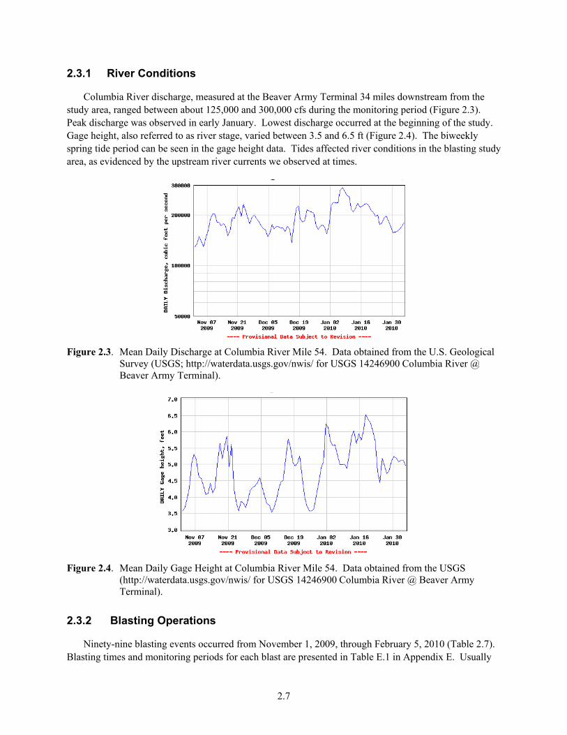
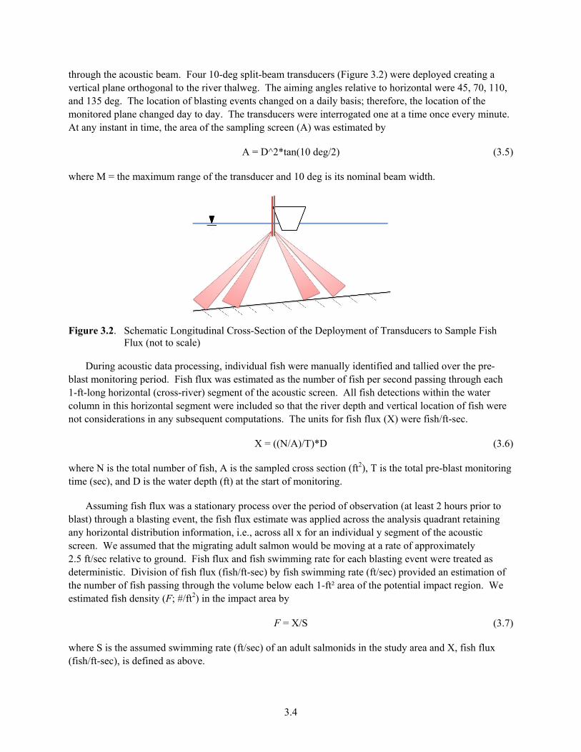
2.3.1 River Conditions

Columbia River discharge, measured at the Beaver Army Terminal 34 miles downstream from the study area, ranged between about 125,000 and 300,000 cfs during the monitoring period (Figure 2.3). Peak discharge was observed in early January. Lowest discharge occurred at the beginning of the study. Gage height, also referred to as river stage, varied between 3.5 and 6.5 ft (Figure 2.4). The biweekly spring tide period can be seen in the gage height data. Tides affected river conditions in the blasting study area, as evidenced by the upstream river currents we observed at times.

Figure 2.3. Mean Daily Discharge at Columbia River Mile 54. Data obtained from the U.S. Geological

Survey (USGS; http://waterdata.usgs.gov/nwis/ for USGS 14246900 Columbia River @ Beaver Army Terminal).

Figure 2.4. Mean Daily Gage Height at Columbia River Mile 54. Data obtained from the USGS

(http://waterdata.usgs.gov/nwis/ for USGS 14246900 Columbia River @ Beaver Army Terminal).

2.3.2 Blasting Operations

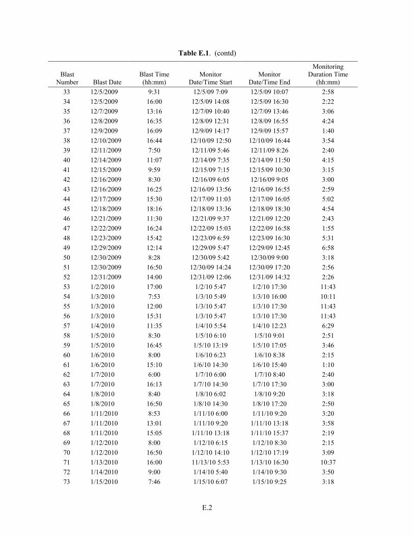
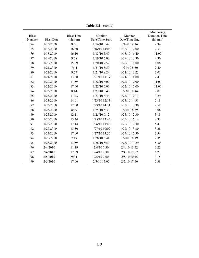
Ninety-nine blasting events occurred from November 1, 2009, through February 5, 2010 (Table 2.7). Blasting times and monitoring periods for each blast are presented in Table E.1 in Appendix E. Usually

2.8

there were one or two blasts on a given day; on January 23, 2010, the blasting contractor conducted four blasting events. We deployed monitoring for every blast for a total of over 453 h of on-the-water monitoring (Table 2.7). The minimum amount of monitoring for a blasting event was 1 h and 10 min, whereas the maximum was 11 h and 43 min. On average, we monitored for 4 h and 38 min per blast. The average blast occurred at 1 pm.

Table 2.7. Blasting and Monitoring Statistics

Blast Time Monitoring Duration

Total 99 blasts 453 h 48 min Minimum 6:00 am 1 h 10 min Maximum 6:16 pm 11 h 43 min Mean 1:00 pm 4 h 38 min

2.3.3 Observations of Marine Mammals and Diving Birds

Harbor seals were present in the safety zone, 2,000 ft upstream and 2,000 ft downstream of the blast site, throughout the 3-month study period. During 93 of the 99 blasts, at least one marine mammal was observed in the safety zone during the designated 2-h monitoring period. We also observed two California sea lions in the safety zone, one on December 21 and another on December 30, 2009.

Diving birds were present sporadically in the safety zone during monitoring, most commonly cormorants, grebes, and mergansers.

2.3.4 Compliance

No marine mammals were observed within the 500-ft marine mammal monitoring zone at blasting time for any of the blasts (Table 2.8). Four marine mammals were present in the safety zone at blasting time. During post-blast surveys, we recovered three dead sturgeon. We did not observe any dead marine mammals or salmon after the blasts. The estimated take of adult salmon was 0.00 fish (see Chapter 3.0 for details).

Table 2.8. Summary of Compliance Monitoring Results

Monitored Indicator Result Total number of marine mammals observed at blast time

In the 2,000-ft safety zone 4 In the 500-ft marine mammal monitoring zone 0

Total number of sturgeon observations during pre-blast surveys 50 Total number of mortalities observed after the blast

Marine mammals 0 Adult salmon 0 Sturgeon 3 Eulachon 0

Total estimated take of listed adult salmon 0.00 fish

2.9

2.4 Summary and Conclusion

The Warrior Point rock blasting project complied with the permit requirements of the regulating agencies. Compliance monitoring was executed according to plan (Carlson and Johnson 2010). As stipulated in the permit for blasting activities granted by the regulatory agencies, monitoring activities were conducted for all 99 blasts from November 1, 2009, to February 5, 2010. No marine mammals were observed within the 500-ft marine mammal monitoring zone at blasting time for any of the blasts. There was no “take” of listed species, as explained further in the next chapter.

3.1

3.0 Estimation of Take

Underwater blasting operations to remove basalt rock in the Columbia River navigation channel had the potential to injure or kill aquatic animals in the blast impact area. The USACE, in consultation with federal and state resource agencies, conducted monitoring to assess any “take” of fish listed as endangered under the ESA and possibly exposed to the high-energy underwater impulses generated by blasting activity, as stipulated in the CRCIP Biological Opinion (NMFS 2002). In fact, blasting operations were not permitted unless monitoring was in place. Take was defined as the number of fish that died as a result of underwater blasting. The National Marine Fisheries Service (NMFS) established acceptable take to be no more than 10 adult and 50 juvenile listed salmonids for all blasting events combined. To minimize take, blasting operations were conducted during a time of year (late fall and winter) when relatively few salmon were expected to be in the study area, but even so, both listed and unlisted juvenile and adult salmonids could be transiting through the impact area during blasting events. Therefore, an approach for determining the take of listed salmonids that was acceptable to the regulatory agencies had to be developed and implemented, thereby allowing the CRCIP to proceed.

We did not have sufficient data to accurately predict a priori the numbers of juvenile and adult salmonids likely to be exposed to blasting. Based on adult passage counts at Bonneville and Willamette Falls dams, the greatest risk of exposure was expected to be to chum salmon (Oncorhynchus keta) in November and December, with some possibility for adult Chinook salmon (O. tshawytscha) and steelhead (O. mykiss) in the impact area. For juvenile salmonids, a review of available information showed that during November, December, and into January these fish were not likely to be actively migrating through the study area (Geist and Currie 2006; Friesen et al. 2007; Keller 2007; Tomaro et al. 2007, 2008; Johnson et al. 2008). However, juvenile fish could be present rearing in the near-shore, shallow waters of the study area (Johnson et al. 2010). This information suggested that fish monitoring during November, December, and into January should focus on adult salmonids, transitioning to juvenile salmonids when emergence and migration of juvenile chum salmon had begun and their occurrence in the study area was more probable. As it turned out, blasting operations were completed before the juvenile chum salmon emigration, which commenced in late January peaked in late February to late March (Arntzen and Murray 2011). Therefore, take estimation concerned only adult salmonids in the blast impact area.

Emergence timing estimates made using temperature monitoring data ranged from the end of January (for earliest emergence) to early April (for 90% emergence). Peak emergence estimates ranged from late February to late March.

We considered physical capture methods to determine the take of adult salmonids, but concluded that physical capture of injured, moribund, and dead salmonids following a blasting event would likely be problematic because of the physical challenges of working with nets (e.g., tow, purse, gill) in a large river (Keevin et al. 2002). The difficulty would be compounded because it was possible the sampling method itself might injure or kill fish. Also, other investigators experienced problems recovering fish injured during a blast or picking them from the water before they were taken by birds or sank (Munday et al. 1986). Carlson and Johnson (2010) reviewed the advantages and disadvantages of seven different physical capture techniques and concluded none would be acceptable for the purpose of blast take estimation. Because direct physical capture of fish, other than those recovered from the surface following a blast, was not without significant disadvantages, an indirect dose-exposure-response technique for take estimation was warranted.

3.2

In this chapter, we describe the dose-exposure-response method we developed to estimate the take of adult salmonids and present the take results for underwater blasting at Warrior Point in the Columbia River from November 1, 2009, through February 5, 2010.

3.1 Methodology

Take estimation involved four elements: 1) estimating the level of impulsive sound to which fish were exposed (dose), 2) estimating the probable number of fish exposed to impulsive sound (exposure), 3) estimating the consequences of that exposure (response), and 4) estimating take (Figure 3.1).

a) Dose: Isopleths of Sound Pressure b) Exposure: Fish Flux

c) Response: Mortality Curve d) Response: Isopleths of Mortality Probability

e) Take Estimation

Figure 3.1. Schematic of the Dose-Exposure-Response Approach for Take Estimation

3.1.1 Dose

The blasting contractor provided the USACE with a measure of the peak pressure generated by each blasting event at a position 10 ft above the bottom and a range of 140 ft from the blasting location. This was the only information we were given by the USACE to estimate the exposure of fish to blast energy.

Blast Blast

Sound pressure

Mor

talit

y

1.

0

1.0

0.8

0.6

Blast

over area = Fish take

Blast

3.3

A consultant to the USACE used equations developed by Cole (1948) to estimate the peak pressure (P) and impulse (I) generated by blasting events as a function of range (R) from the blasting event and the equivalent weight of explosive (W) used for the blast. The consultant also used a scaling factor (k = 0.14) to account for the reduction in peak pressure and impulse because the explosive charges were buried in rock and covered by stemming consisting of a layer of pea gravel approximately 2 ft thick deposited on top of the explosive array prior to discharge. The equations were

P = k × 22500 × (W13

R)1.13 (3.1)

I = k × 2180 × �W13� × (W

13

R)1.05 (3.2)

where P = peak pressure in psi W = charge weight in lb R = range from the blasting event in ft K = scaling factor for buried blast = 0.14.

We derived an equation to provide estimates of impulse (I) given the radial distance from a blasting event (R) for each blasting event by solving Equation (1) for charge weight (W) given the single observation of peak pressure (P) provided by the blasting contractor at R = 140 ft, letting k = 0.14 and substituting the value of W into Equation (2).

W = (( P3150

)1

1.13 × R)3 (3.3)

The impact region (2D – plan view) within which impulsive sound created by blasting may affect adult salmonids was modeled as a square with dimensions of 200 ft by 200 ft with divisions into 40,000 smaller 1-ft² sections. The squares were indexed for computation purposes using a rectangular coordinate system with the origin in the center of the total region of interest. The origin was also the center of blasting events. The x axis was parallel to the river thalweg. The radial distance (R) from a blasting event for each 1-ft² cell in the impact region model was then estimated by

R = �x2 + y2 (3.4)

where (xi,yi) are the rectangular coordinates for the ith 1-ft² element of the potential impact region. The x axis is along the river thalweg and the y axis is cross-channel.

Impulse (I) was estimated for each cell by using Equation (2) and the estimated radial distance (R) of the cell from the blasting event. The actual dose was more complicated than the simple computation given suggests. However, given the lack of information for response of fish to impulsive sound, this method for estimating dose was adequate.

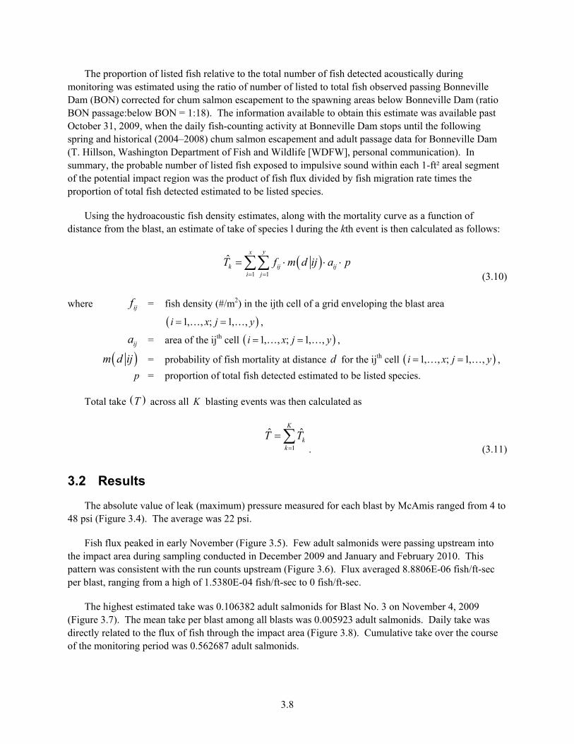
3.1.2 Exposure

Sampling for adult salmonids was conducted from the research vessel Strait Science anchored approximately 500 ft downstream of the blast site. A split-beam hydroacoustic system enabled us to measure the relative size of the fish, location within the ensonified beam, and direction of movement

3.4

through the acoustic beam. Four 10-deg split-beam transducers (Figure 3.2) were deployed creating a vertical plane orthogonal to the river thalweg. The aiming angles relative to horizontal were 45, 70, 110, and 135 deg. The location of blasting events changed on a daily basis; therefore, the location of the monitored plane changed day to day. The transducers were interrogated one at a time once every minute. At any instant in time, the area of the sampling screen (A) was estimated by

A = D^2*tan(10 deg/2) (3.5)

where M = the maximum range of the transducer and 10 deg is its nominal beam width.

Figure 3.2. Schematic Longitudinal Cross-Section of the Deployment of Transducers to Sample Fish

Flux (not to scale)

During acoustic data processing, individual fish were manually identified and tallied over the pre-blast monitoring period. Fish flux was estimated as the number of fish per second passing through each 1-ft-long horizontal (cross-river) segment of the acoustic screen. All fish detections within the water column in this horizontal segment were included so that the river depth and vertical location of fish were not considerations in any subsequent computations. The units for fish flux (X) were fish/ft-sec.

X = ((N/A)/T)*D (3.6)

where N is the total number of fish, A is the sampled cross section (ft2), T is the total pre-blast monitoring time (sec), and D is the water depth (ft) at the start of monitoring.

Assuming fish flux was a stationary process over the period of observation (at least 2 hours prior to blast) through a blasting event, the fish flux estimate was applied across the analysis quadrant retaining any horizontal distribution information, i.e., across all x for an individual y segment of the acoustic screen. We assumed that the migrating adult salmon would be moving at a rate of approximately 2.5 ft/sec relative to ground. Fish flux and fish swimming rate for each blasting event were treated as deterministic. Division of fish flux (fish/ft-sec) by fish swimming rate (ft/sec) provided an estimation of the number of fish passing through the volume below each 1-ft² area of the potential impact region. We estimated fish density (F; #/ft2) in the impact area by

F = X/S (3.7)

where S is the assumed swimming rate (ft/sec) of an adult salmonids in the study area and X, fish flux (fish/ft-sec), is defined as above.

3.5

3.1.3 Response

The response model for adult salmonids was based on the findings of Yelverton (1975). Yelverton’s report is one of the most frequently cited works for evaluation of the probable response of fish with swim bladders to impulsive sound. In it, probit equations for the sizes of test fish are detailed. We extracted pertinent equations (Table 3.1) from the report and verified their parameters prior to using them in our take-estimation methodology. The probit equations allowed us to estimate the impulse (exposure) for probability of mortality over the range from 0.01 to 0.99 for all sizes of fish tested by Yelverton (1975). A resulting matrix of log base-10-transformed impulse values by log-transformed fish mass and probability of mortality was then used as the data source to fit linear equations (y = log impulse, x = log fish mass) for several probability of mortality values. The resulting equations were solved for an adult salmonid fish mass of 4,536 g (10 lb) to obtain a matrix of paired values for impulse and probability of mortality.

Table 3.1. Probit Equations for the Relationship Between Impulsive Sound Pressure and Fish Response (from Yelverton 1975)

Species Mean Wt in

Grams Impulse psi-msec

Probit Equation LD1 LD50 LD99 Top minnow 0.47 1.3 3.4 8.9 y = 2.089 + 5.516 * log x Small goldfish 1.4 3 6.2 12.5 y = -0.976 + 7.557 * log x Small channel catfish 105 17.6 33.3 63 y = -7.781 + 8.395 * log x Small carp 149 19 27.4 39.5 y = -16.119 + 14.686 * log x Small carp 117 16.7 23.5 33.1 y = -14.440 + 15.644 * log x Small carp 113 14.9 26.2 46.2 y = -8.385 + 9.445 * log x Rainbow trout 143 12.3 20.7 35 y = -8.436 + 10.207 * log x Large goldfish 245 13 26.5 53.8 y = -5.766 + 7.557 * log x Large channel catfish 338 19.5 26.8 59.7 y =-8.11 + 8.39 * log x Large carp 711 35.1 48.5 69.7 y = -21.511 + 15.644 * log x Guppy fry 0.02 0.7 1.7 y = 3.687 + 5.516 * log x Guppy adult 0.13 1 2.7 7.2 y =2.603 + 5.516 * log x Small bluegill 1.4 4.3 6.7 10.4 y = -3.063 + 12.174 * log x Large bluegill 88 17.7 20.7 24.3 y = -40.078 + 34.231 * log x Largemouth bass 146 18.8 26.5 57.3 y = -17 + 15.644 * log x LD1, LD50, and LD99 = dosage required to kill 1%, 50%, or 99%, respectively, of the test population.

The logit values for the probabilities of mortality for the range of impulses of interest were calculated and the parameters for a logistic function relating impulse and probability of mortality were estimated using linear regression. The data and linear regression used to estimate the logistic function parameters are shown below (Tables 3.2 and 3.3, respectively).

3.6

Table 3.2. Logit Values for the Probabilities of Mortality for the Range of Impulses of Interest

Impulse Log Impulse Log Prob Mort Prob Mort Logit Logistic Prob

Mort 60.00 1.78 -2.04 0.01 -4.69134 0.0164 62.00 1.79 -1.74 0.02 -3.97763 0.0240 64.00 1.81 -1.47 0.03 -3.35038 0.0350 66.00 1.82 -1.24 0.06 -2.79578 0.0508 68.00 1.83 -1.04 0.09 -2.30142 0.0733 70.00 1.85 -0.87 0.14 -1.8563 0.1045 72.00 1.86 -0.72 0.19 -1.45079 0.1470 74.00 1.87 -0.59 0.25 -1.07651 0.2029 76.00 1.88 -0.49 0.33 -0.72619 0.2732 78.00 1.89 -0.39 0.40 -0.39349 0.3569 80.00 1.90 -0.32 0.48 -0.07285 0.4504 82.00 1.91 -0.25 0.56 0.240801 0.5475 84.00 1.92 -0.20 0.63 0.552137 0.6412 86.00 1.93 -0.15 0.70 0.8657 0.7252 88.00 1.94 -0.12 0.77 1.186081 0.7958 90.00 1.95 -0.09 0.82 1.518154 0.8519 92.00 1.96 -0.06 0.87 1.867336 0.8947 94.00 1.97 -0.04 0.90 2.239903 0.9262 96.00 1.98 -0.03 0.93 2.643335 0.9488 98.00 1.99 -0.02 0.96 3.086572 0.9647

100.00 2.00 -0.01 0.97 3.579614 0.9758 102.00 2.01 -0.01 0.98 4.13024 0.9835 104.00 2.02 0.00 0.99 4.72973 0.9888 106.00 2.03 0.00 1.00 5.306357 0.9924

Table 3.3. Linear Regression Used to Estimate the Logistic Function Parameters

Regression Statistics Multiple R 0.995632 R Square 0.991282 Adjusted R Square 0.990886 Standard Error 0.264265 Observations 24 ANOVA

df SS MS F Significance F Regression 1 174.7035 174.7035 2501.618 3.73E-24 Residual 22 1.536396 0.069836

Total 23 176.2399

Coefficients Standard

Error t Stat P-value Lower 95% Upper 95%

Lower 95.0% Upper 95.0%

Intercept -15.7897 0.327868 -48.1586 8.52E-24 -16.4696 -15.1097 -16.4696 -15.10970036 X Variable 1 0.194882 0.003896 50.01618 3.73E-24 0.186801 0.202963 0.186801 0.202962649

The equation for the derived logistic function and a plot (Figure 3.3) of the function follow:

𝑃𝑟𝑜𝑏𝑎𝑏𝑖𝑙𝑖𝑡𝑦 𝑜𝑓 𝑀𝑜𝑟𝑡𝑎𝑙𝑖𝑡𝑦 =𝑒−15.7897+0.19488×𝐼𝑚𝑝𝑢𝑙𝑠𝑒

1 + 𝑒−15.7897+0.19488×𝐼𝑚𝑝𝑢𝑙𝑠𝑒

3.7

Figure 3.3. Logistic Relationship Between Blast Impulse and Probability of Mortality for Adult

Salmonids

3.1.4 Take

The fundamental relationship used to estimate take ( )T was as follows:

( )fish density area mortalityT P= × × (3.8)

where the product of fish density × area is the number of fish at risk in an area and where the probability of mortality due to impulsive sound exposure measures the degree of risk. In practice, this take equation was more complex, allowing fish density and probability of mortality to be location-specific. Thus, total take for a blasting event will be the sum of the location-specific estimates of take iT , that is:

( ) ( )

1 1fish density area mortality

N N

i ii ii i

T T P= =

= = × ×∑ ∑. (3.9)

We assumed that sound generated by the blast propagated radially and symmetrically from its origin following the loss function provided to the Corps by the blasting contractor. Under this assumption, which is not strictly true, the four quadrants within the coordinate system were symmetrical so only one quadrant need be considered to estimate the sound exposure that fish located in each of the 1-ft² areas would experience. In addition, the flux of fish was assumed to be symmetrical for + and – y, which seems to be the case for adult fish. Therefore, take can be estimated by modeling one quadrant, estimating take for the quadrant, and multiplying by 4.

0.00

0.10

0.20

0.30

0.40

0.50

0.60

0.70

0.80

0.90

1.00

40.00 50.00 60.00 70.00 80.00 90.00 100.00 110.00 120.00

Prob

abili

ty o

f Mor

talit

y

Impulse in psi-ms

Response Function for 4,536 gram Fish

3.8

The proportion of listed fish relative to the total number of fish detected acoustically during monitoring was estimated using the ratio of number of listed to total fish observed passing Bonneville Dam (BON) corrected for chum salmon escapement to the spawning areas below Bonneville Dam (ratio BON passage:below BON = 1:18). The information available to obtain this estimate was available past October 31, 2009, when the daily fish-counting activity at Bonneville Dam stops until the following spring and historical (2004–2008) chum salmon escapement and adult passage data for Bonneville Dam (T. Hillson, Washington Department of Fish and Wildlife [WDFW], personal communication). In summary, the probable number of listed fish exposed to impulsive sound within each 1-ft² areal segment of the potential impact region was the product of fish flux divided by fish migration rate times the proportion of total fish detected estimated to be listed species.

Using the hydroacoustic fish density estimates, along with the mortality curve as a function of distance from the blast, an estimate of take of species l during the kth event is then calculated as follows:

( )

1 1

ˆyx

k ij iji j

T f m d ij a p= =

= ⋅ ⋅ ⋅∑∑ (3.10)

where ijf = fish density (#/m2) in the ijth cell of a grid enveloping the blast area

( )1, , ; 1, ,i x j y= = ,

ija = area of the ijth cell ( )1, , ; 1, ,i x j y= = ,

( )m d ij = probability of fish mortality at distance d for the ijth cell ( )1, , ; 1, ,i x j y= = ,

p = proportion of total fish detected estimated to be listed species.

Total take ( )T across all K blasting events was then calculated as

1

ˆ ˆK

kk

T T=

=∑. (3.11)

3.2 Results

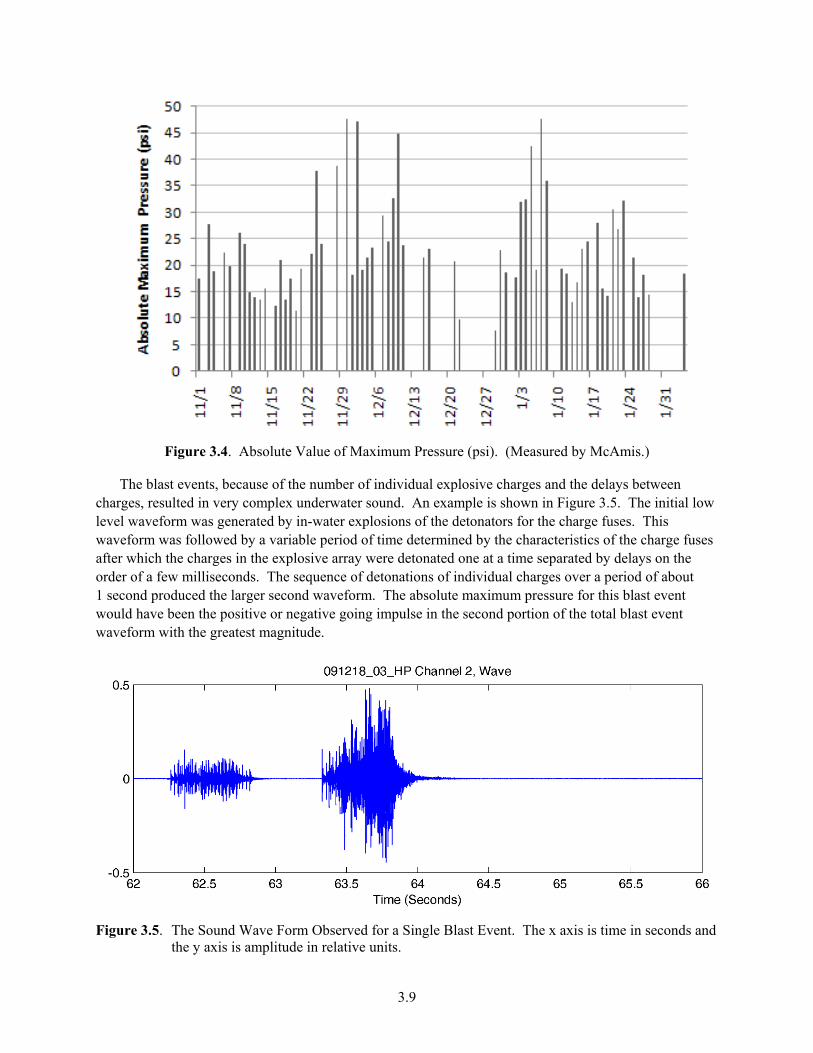
The absolute value of leak (maximum) pressure measured for each blast by McAmis ranged from 4 to 48 psi (Figure 3.4). The average was 22 psi.

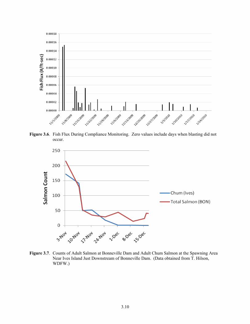
Fish flux peaked in early November (Figure 3.5). Few adult salmonids were passing upstream into the impact area during sampling conducted in December 2009 and January and February 2010. This pattern was consistent with the run counts upstream (Figure 3.6). Flux averaged 8.8806E-06 fish/ft-sec per blast, ranging from a high of 1.5380E-04 fish/ft-sec to 0 fish/ft-sec.

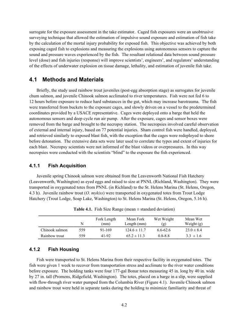
The highest estimated take was 0.106382 adult salmonids for Blast No. 3 on November 4, 2009 (Figure 3.7). The mean take per blast among all blasts was 0.005923 adult salmonids. Daily take was directly related to the flux of fish through the impact area (Figure 3.8). Cumulative take over the course of the monitoring period was 0.562687 adult salmonids.

3.9

Figure 3.4. Absolute Value of Maximum Pressure (psi). (Measured by McAmis.)

The blast events, because of the number of individual explosive charges and the delays between charges, resulted in very complex underwater sound. An example is shown in Figure 3.5. The initial low level waveform was generated by in-water explosions of the detonators for the charge fuses. This waveform was followed by a variable period of time determined by the characteristics of the charge fuses after which the charges in the explosive array were detonated one at a time separated by delays on the order of a few milliseconds. The sequence of detonations of individual charges over a period of about 1 second produced the larger second waveform. The absolute maximum pressure for this blast event would have been the positive or negative going impulse in the second portion of the total blast event waveform with the greatest magnitude.

Figure 3.5. The Sound Wave Form Observed for a Single Blast Event. The x axis is time in seconds and

the y axis is amplitude in relative units.

3.10

Figure 3.6. Fish Flux During Compliance Monitoring. Zero values include days when blasting did not

occur.

Figure 3.7. Counts of Adult Salmon at Bonneville Dam and Adult Chum Salmon at the Spawning Area

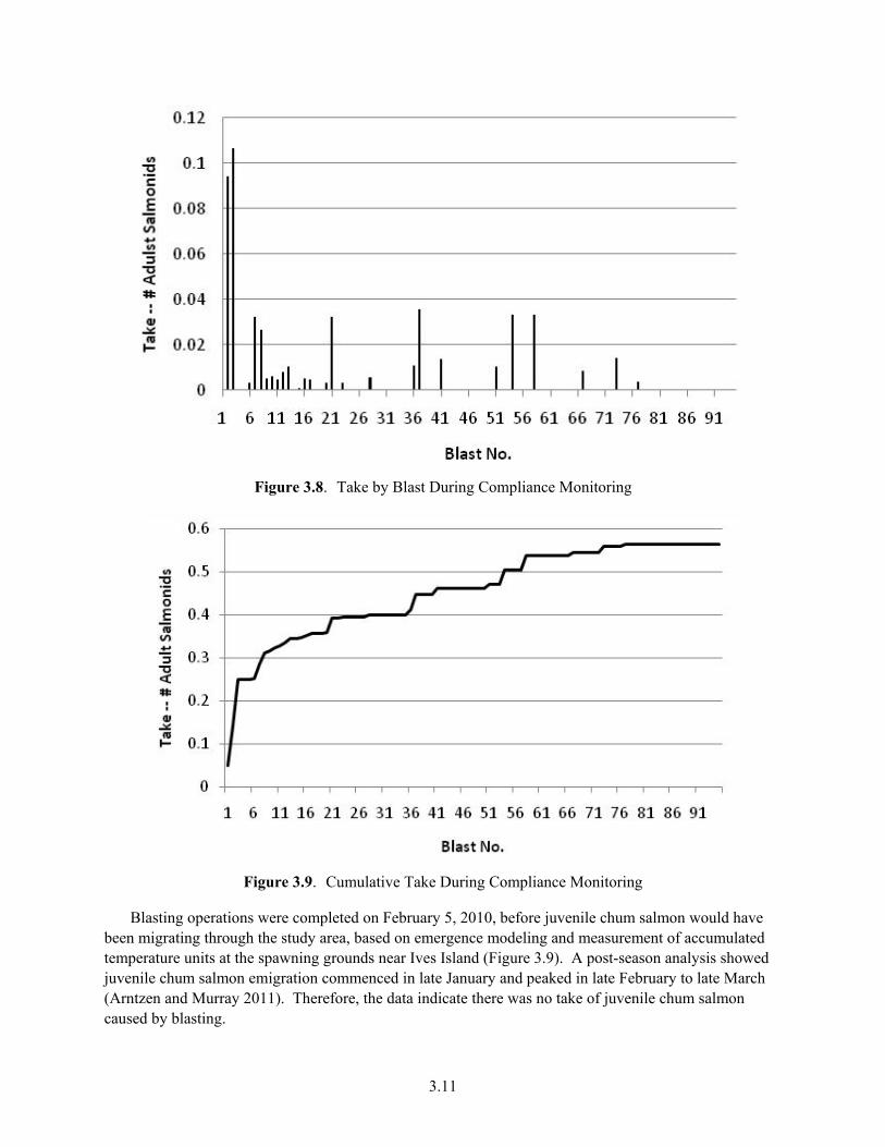
Near Ives Island Just Downstream of Bonneville Dam. (Data obtained from T. Hilson, WDFW.)

3.11

Figure 3.8. Take by Blast During Compliance Monitoring

Figure 3.9. Cumulative Take During Compliance Monitoring

Blasting operations were completed on February 5, 2010, before juvenile chum salmon would have been migrating through the study area, based on emergence modeling and measurement of accumulated temperature units at the spawning grounds near Ives Island (Figure 3.9). A post-season analysis showed juvenile chum salmon emigration commenced in late January and peaked in late February to late March (Arntzen and Murray 2011). Therefore, the data indicate there was no take of juvenile chum salmon caused by blasting.

3.12

Figure 3.10. Accumulated Temperature Units (ATUs) and Estimated Emergence Timing for Chum

Salmon at Ives Island (provided by E. Arntzen, PNNL)

3.3 Summary and Conclusion

Cumulative take of juvenile and adult salmon was less than that permitted by the regulating agencies and, therefore, the blasting project met the requirements established by regulators. Blasting occurred after most of the adult salmon migration had passed the study area and was completed before juvenile chum salmon arrived. The dose-exposure-response approach to estimating take provided an unobtrusive, science-based method that allowed near real-time reporting of results as required by the regulators.

4.1

4.0 Response of Caged Juvenile Salmonids to High-Energy Impulsive Sound

Underwater explosions are often a result of needed construction, demolition, rock excavation, waterway applications (e.g., channel alterations, dike removal), military operations, and fishing activities. The chemical and physical parameters of underwater blasting agents and explosions are fairly well understood. Conversely, the sound and pressure waves resulting from the explosion are complex (Urick 1996). To unravel the complexity of the resultant sound and pressure waves, information is needed about the type and weight of explosives (i.e., charge and blast timing, charge and blast weights, rock material, and design such as number, depth, and spacing of holes) and energy released from the explosion (i.e., amplitude, frequency, duration, pressure, impulse, energy flux density [Mellor 1986; Urick 1996]). Besides the sound and pressure waves produced by the explosion, other byproducts are projectiles and gaseous chemical products, which are vented to the air from the water upheaval (Mellor 1986). These byproducts of underwater explosions can have deleterious impacts on the local animals, habitat, and structures near the blast.

The USACE, in consultation with federal and state resource agencies, needed to monitor and assess any “take” of fish listed as endangered under the ESA exposed to the high-energy underwater impulses generated by blasting activity, as stipulated in the CRCIP Biological Opinion (NMFS 2002). Regulatory agencies, such as the National Oceanic and Atmospheric Administration, do not permit underwater rock blasts (or blasts near aquatic environments) without mitigation of the adverse sound and pressure effects. Initial estimates of the underwater peak pressure and impulse to be generated by underwater rock blasting indicated that the affected area (where there was risk of injury by percussion and impulsive decompression for a 90-lb charge weight) could extend approximately 700 ft radially out from the location of the charge weight (Communication USACE-Portland District, Microsoft Excel Spreadsheet: Columbia River Blast Pressure Impulse Attenuation Calculation R2.xls). The NMFS established acceptable take to be no more than 10 adult and 50 juvenile listed salmonids for all blast events combined. To minimize take, blasting operations were conducted during a time of year (late fall and winter) when relatively few salmon were expected to be in the study area, but even so, both listed and unlisted juvenile and adult salmonids, sturgeon, and eulachon could be transiting through the impact area during blast events.

To monitor fish take, immediate mortality is the only response state readily detectable (i.e., observable); however, it can only be assessed if the fish can be recovered and examined immediately after exposure. Given the turbidity and outgoing flow rate of the Columbia River, heavy vessel traffic, and large monitoring area, it would be difficult to detect fish mortality injured or terminated by the blast exposures (Carlson et al. 2007). In addition, not all injuries resulting from sound and pressure waves are mortal, but require time for expression, resulting in non-lethal effects such as reduced fitness or increased susceptibility to predation. To effectively monitor for “take,” this project included assessments of direct and indirect mortality from underwater rock blasting (Carlson and Johnson 2010).

In this chapter, we describe the fish cage exposures that provided data to the “take estimation” model (see Chapter 3.0 for a description of the take estimator), and further define criteria for physiological damage to fishes exposed to underwater explosions at Warrior Point in the Columbia River from November 1, 2009, through February 5, 2010. Because physical capture of fish, other than those recovered from the surface following a blast, had significant disadvantages, caged fish were used as a

4.2

surrogate for the exposure assessment in the take estimator. Caged fish exposures were an unobtrusive surveying technique that allowed the estimation of impulsive sound exposure and estimation of fish take by the calculation of the mortal injury probability for exposed fish. This objective was achieved by both exposing caged fish to explosions and measuring the explosions using autonomous sensors to capture the sound and pressure waves experienced by the fish. The resultant relational data between sound pressure level (dose) and fish injuries (response) will improve scientists’, engineers’, and regulators’ understanding of the effects of underwater explosion on tissue damage, lethality, and estimation of juvenile fish take.

4.1 Methods and Materials

Briefly, the study used rainbow trout juveniles (post-egg absorption stage) as surrogates for juvenile chum salmon, and juvenile Chinook salmon acclimated to river temperatures. Fish were not fed 6 to 12 hours before exposure to reduce hard substances in the gut, which may increase barotrauma. The fish were transferred from buckets to the exposure cages, and slowly driven on a vessel to the predetermined coordinates provided by a USACE representative. Cages were deployed onto a barge that held the autonomous sensors and deep cycle run air pump. After the exposure, cages and sensor boxes were removed from the barge and brought to the necropsy station. The necropsies involved careful observation of external and internal injury, based on 77 potential injuries. Sham control fish were handled, deployed, and retrieved similarly to exposed blast fish, with the exception that the cages were redeployed to shore before detonation. The extensive data sets were later used to correlate the types and extent of injuries for each blast. Necropsy scientists were not informed of the blast videos or overpressures. In this way necropsies were conducted with the scientists “blind” to the exposure the fish experienced.

4.1.1 Fish Acquisition

Juvenile spring Chinook salmon were obtained from the Leavenworth National Fish Hatchery (Leavenworth, Washington) as eyed eggs and raised to size at PNNL (Richland, Washington). They were transported in oxygenated totes from PNNL (in Richland) to the St. Helens Marina (St. Helens, Oregon, 4.3 h). Juvenile rainbow trout (O. mykiss) were transported in oxygenated totes from Trout Lodge Hatchery (Trout Lodge, Soap Lake, Washington) to St. Helens Marina (St. Helens, Oregon, 5.16 h).

Table 4.1. Fish Size Range (mean ± standard deviation)

N Fork Length

(mm) Mean Fork

Length (mm) Wet Weight

(g) Mean Wet Weight (g)

Chinook salmon 559 91-169 124.6 ± 11.7 6.6-62.6 23.0 ± 8.4 Rainbow trout 559 41-92 65.2 ± 11.3 0.8-8.8 3.3 ± 1.6

4.1.2 Fish Housing

Fish were transported to St. Helens Marina from their respective facility in oxygenated totes. The fish were given 1 week to recover from transportation stress and acclimate to the river water conditions before exposure. The holding tanks were four 177-gal Bonar totes measuring 45 in. long by 40 in. wide by 27 in. tall (Promens, Ridgefield, Washington). The totes, placed on a barge in a slip, were supplied with flow-through river water pumped from the Columbia River (Figure 4.1). Juvenile Chinook salmon and rainbow trout were held in separate tanks during the holding to minimize familiarity and threat of

4.3

predation stress. Fish were fed pellet and flake feed twice daily at 1.1% of their body weight (BioVita, Bio-Oregon, Oregon). All totes were siphoned twice daily to remove any silt, feces, and other debris. The totes were retrofitted with screen mesh tops to allow for a natural photoperiod.

Figure 4.1. Holding Totes Used in This Study for Pre- and Post-Exposure Fish. Totes were plumbed to

have free-flowing river water.

After exposure to blasting conditions, a subset of fish in each cage was retained to monitor for injury and mortality over a 48-hour period. Each cohort was held in a separate Bonar tote inside a 5-gal lidded bucket with holes drilled along the entire top half of the bucket. This configuration allowed the fish to remain separated from other cohorts, but to have access to adequate water flow.

4.1.3 Caged Fish Deployment

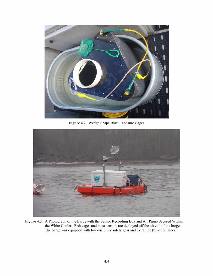
Caged fish exposures were conducted to assess the physiological impacts on two species: juvenile Chinook salmon and rainbow trout. The caged fish exposures were designed to assess the effects of fish exposed to different sound levels created by the underwater rock blasting conducted. Fish were not fed for 6 to 12 hours before exposure to reduce hard substances in the gut, which may increase observed barotrauma. The fish were transferred from buckets into the exposure cages (0.6 m x 0.6 m x 0.6 m, 0.11 m3, 29 gal) that sat on a vessel in a trough filled with 30 gal of fresh river water. The cages were specially designed for high-velocity conditions, yet maintained air in the top 5 cm (or 2 in., excluding the white cuff of the lid, Figure 4.2) for fish to fill their swim bladders. The cages provided flow relief. The front edge was a solid baffle (approximately 25 cm long), and the remaining sides were screen mesh. The cages were slowly driven on a vessel to the predetermined coordinates provided by a USACE representative.

Cages were deployed onto an anchored barge that held the autonomous sensors and an air pump connected to a deep cycle battery (Figure 4.3). The pressure transducer cables were hooked onto the cage and air lines were connected to the cage. Once the cages were underwater, the pressure transducer system was activated (see description below). The cages were monitored for air expression over the pre-blast acclimation period. The cage acclimation period began once the fish were deployed off the barge and ranged from 1 to 6 hours depending on vessel traffic and difficulties experienced by the blasting contractors.

4.4

Figure 4.2. Wedge Shape Blast Exposure Cages

Figure 4.3. A Photograph of the Barge with the Sensor Recording Box and Air Pump Secured Within

the White Cooler. Fish cages and blast sensors are deployed off the aft end of the barge. The barge was equipped with low-visibility safety gear and extra line (blue container).

4.5

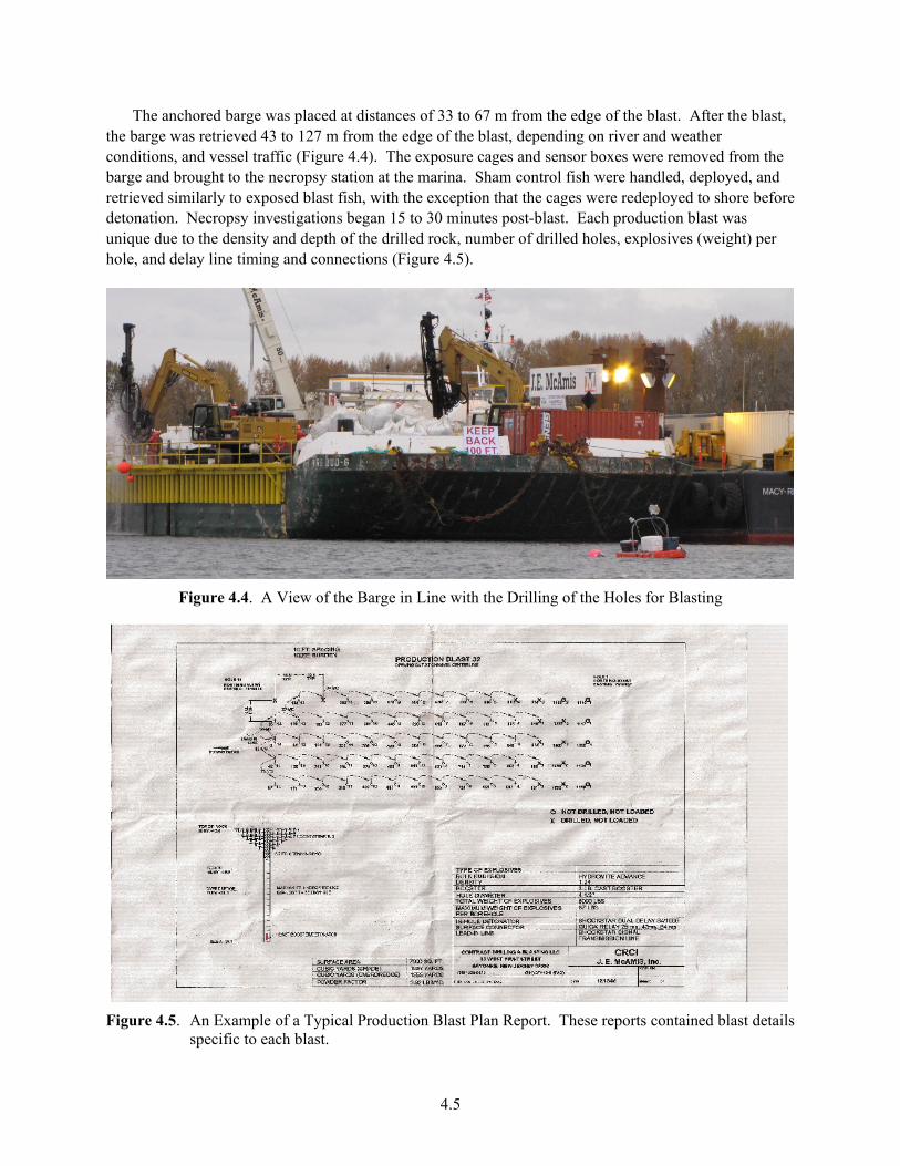
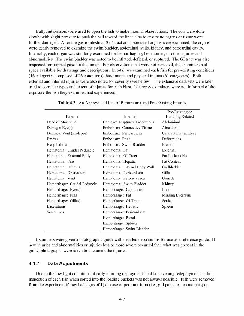
The anchored barge was placed at distances of 33 to 67 m from the edge of the blast. After the blast, the barge was retrieved 43 to 127 m from the edge of the blast, depending on river and weather conditions, and vessel traffic (Figure 4.4). The exposure cages and sensor boxes were removed from the barge and brought to the necropsy station at the marina. Sham control fish were handled, deployed, and retrieved similarly to exposed blast fish, with the exception that the cages were redeployed to shore before detonation. Necropsy investigations began 15 to 30 minutes post-blast. Each production blast was unique due to the density and depth of the drilled rock, number of drilled holes, explosives (weight) per hole, and delay line timing and connections (Figure 4.5).

Figure 4.4. A View of the Barge in Line with the Drilling of the Holes for Blasting

Figure 4.5. An Example of a Typical Production Blast Plan Report. These reports contained blast details

specific to each blast.

4.6

4.1.4 Sham Fish

Sham fish (n = 24) were deployed similarly to blast-exposed fish. After a minimum of 3 hours exposure to the cage and river, yet not exposed to a blast, the cages were retrieved and the fish necropsied. The use of sham fish ensured that tissue damages incurred from transportation and handling stressors were documented. The fish were then euthanized and examined in the same manner as the blast-exposed fish.

4.1.5 Pressure Recording and Analysis

The pressure transducer system consisted of pressure sensors (Model # 138A01, Piezotronics, Depew, NY), cabling, a power amplifier, a digital audio recorder (PCM-D50, Sony Corporation, New York, NY), and external file storage. All transducer data were adjusted for each individual transducer’s calibration. A pretest calibration was conducted on each sensor. The pressure transducer systems received through-system checks that were also used for correcting the recorded signals.

Once deployed, the system functionality was verified by banging the vessel and monitoring the signal on the digital recorder. Depending on the time, the recorder was either left in the record position or paused for later start. All paused signal recording units were started a minimum of 15 minutes prior to the blast.

The following parameters were calculated from the recorded charge and blast signals: peak positive pressure (Pa), peak negative pressure (Pa), peak absolute pressure (Pa), root-mean-square (RMS) pressure (Pa), main frequency (Hz), main frequency amplitude (Pa), and duration (s). In addition, the total RMS pressure (Pa) and total power were estimated from the combination of the detonator and explosive charge signals.

4.1.6 Necropsy

A total of 1118 fish were examined after exposure to the blasts. Once the fish arrived at the necropsy station at the marina, the sample was separated into three equal groups: fish to be examined immediately, and fish to be examined 24 hours and 48 hours after the blast exposure. Fish to be examined immediately were carried to the necropsy station in a water-filled 5-gal bucket with air bubbling. The remaining fish to be held for 24 or 48 hours were placed into a labeled 5-gal bucket and returned to the appropriate holding tote.

At the necropsy station, fish were euthanized one at a time by exposure to pH-balanced tricaine methanesulfonate (250 mg L-1 water) solution. Just prior to and during the initial stages of euthanasia, examiners noted signs of negative or positive buoyancy, eradicated or stunned behavior, and/or hyperactive chromatophore activity. When respiration ceased, fish were removed, weighed (wet [WW] g) and measured (fork length [FL] mm). The blast number and cage depth were recorded along with a unique fish identification number. A detailed necropsy was performed to examine each fish for the presence of any abnormalities. Externally, the eyes, fins, skin, gills, pericardial window, and inside the mouth were examined for abrasions, lacerations, hemorrhaging, hematoma, and other injuries or abnormities.

4.7

Ballpoint scissors were used to open the fish to make internal observations. The cuts were done slowly with slight pressure to push the ball toward the linea alba to ensure no organs or tissue were further damaged. After the gastrointestinal (GI) tract and associated organs were examined, the organs were gently removed to examine the swim bladder, abdominal walls, kidney, and pericardial cavity. Internally, each organ was similarly examined for hemorrhaging, hematomas, or other injuries and abnormalities. The swim bladder was noted to be inflated, deflated, or ruptured. The GI tract was also inspected for trapped gases in the lumen. For observations that were not expected, the examiners had space available for drawings and descriptions. In total, we examined each fish for pre-existing conditions (16 categories composed of 26 conditions), barotrauma and physical trauma (61 categories). Both external and internal injuries were also noted for severity (see below). The extensive data sets were later used to correlate types and extent of injuries for each blast. Necropsy examiners were not informed of the exposure the fish they examined had experienced.

Table 4.2. An Abbreviated List of Barotrauma and Pre-Existing Injuries

External Internal Pre-Existing or

Handling Related Dead or Moribund Damage: Ruptures, Lacerations Abdominal Damage: Eye(s) Embolism: Connective Tissue Abrasions Damage: Vent (Prolapse) Embolism: Pericardium Cataract Flatten Eyes Emesis Embolism: Renal Deformities Exopthalmia Embolism: Swim Bladder Erosion Hematoma: Caudal Peduncle Hematoma: Fat External Hematoma: External Body Hematoma: GI Tract Fat Little to No Hematoma: Fins Hematoma: Hepatic Fat Content Hematoma: Isthmus Hematoma: Internal Body Wall Gallbladder Hematoma: Operculum Hematoma: Pericardium Gills Hematoma: Vent Hematoma: Pyloric caeca Gonads Hemorrhage: Caudal Peduncle Hematoma: Swim Bladder Kidney Hemorrhage: Eye(s) Hemorrhage: Capillaries Liver Hemorrhage: Fins Hemorrhage: Fat Missing Eyes/Fins Hemorrhage: Gill(s) Hemorrhage: GI Tract Scales Lacerations Hemorrhage: Hepatic Spleen Scale Loss Hemorrhage: Pericardium Hemorrhage: Renal Hemorrhage: Spleen Hemorrhage: Swim Bladder

Examiners were given a photographic guide with detailed descriptions for use as a reference guide. If new injuries and abnormalities or injuries less or more severe occurred than what was present in the guide, photographs were taken to document the injuries.

4.1.7 Data Adjustments

Due to the low light conditions of early morning deployments and late evening redeployments, a full inspection of each fish when sorted into the loading buckets was not always possible. Fish were removed from the experiment if they had signs of 1) disease or poor nutrition (i.e., gill parasites or cataracts) or

4.8

2) handling and transportation stress (such as abrasions, torn fins). In addition, fish were not necropsied if they jumped or were dropped during bucket-to-cage or cage-to-bucket transfers.

4.1.8 Injury Descriptions

Injuries are descried relative to barotrauma, mortality, severity, and statistical methods.

4.1.8.1 Barotrauma

Barotrauma is the physical damage caused by a quick decrease or increase from ambient pressure. Barotrauma and related pressure injuries have been documented in a wide range of activities—for example, fish brought from depth to surface water quickly (Scheer et al. 2009), pile driving events (Popper et al. 2006), fish passing through hydroturbines (Carlson and Abernathy 2005), and the use of underwater explosives (Govoni et al. 2003). Due to the inconsistencies or variations among species, experimental designs and blast-related data (see above), four parameters have been identified as likely strong predictors of fish mortality: pressure, impulse, energy density, and denotation velocity, which is defined as the detonation rate of blasting agents.

Barotrauma injuries range from non-lethal to lethal depending on explosion characteristics. Non-lethal injuries could result in altered physiological states, including changes in scale loss, hormone levels, sensory detection, tissue damage, embolisms, and/or changes in behaviors that increase the risk of exposure to predation by piscivorous fish, marine mammals, and avian species (Linton et al. 1985; Popper et al. 2004; Scheer et al. 2009). Barotrauma can be expressed as overinflated or ruptured swim bladders and stomachs, anal or stomach eversions, exophthalmia (bulging eyes), contusions, hemorrhaging, and extreme injuries such as lacerated organs (Linton et al. 1985; Govoni et al. 2003; Hannah and Matteson 2007; Scheer et al. 2009).

Past investigations into underwater rock blasts have documented the swim bladder to be most often the injured organ to varying degrees (Wiley et al. 1981; Linton et al. 1985; Yelverton et al. 1975). Swim bladders are gas-filled organs that are used primarily by fish for buoyancy control, and in some species, secondarily for hearing and/or gas exchange. Rapid sequential changes in pressure cause the swim bladder to contract and overexpand. It has been proposed that the negative pressure (relative to ambient) is responsible for the overexpansion of the swim bladder (Hubbs and Rechnitzer 1952; Wiley et al. 1981). During this process, the pulsating swim bladder may damage itself, and other organs, including local muscle and mesentery tissue, and purge gas into the GI tract.

Barotrauma also occurs through the physical-chemical mechanisms of blood gases supersaturating and leading to emboli and tissue trauma. Gas supersaturation occurs when the partial pressure of one or more gases becomes greater than that of the relative ambient pressure. The blood and tissue of the fish will react quickly to reach equilibrium with its surrounding environment. The difference in gas pressure can cause the gas to leave solution in the fishes’ bloodstream, thereby leaving behind gas bubbles (emboli) that increase the pressure in blood vessels, potentially rupturing the vessels, and can enter organs, such as gills and the fish’s heart and disrupt organ function. The size and location of the emboli will vary depending on the rapid pressure change between ambient positive and negative pressure associated with the underwater blast.

4.9

4.1.8.2 Mortality

The pressure-related mortality of fish has been documented as a result of underwater rock blasts (Wiley et al. 1981), but the exact measurement (waveform) to predict pressure-related mortality is poorly documented. Wiley et al. (1981) indicated that the charge size and distance from detonation were very important in the determination of fish mortality. The water depth, substrate type, and fish species may be confounding factors. The rapid change between high overpressures and high underpressures is likely the primary factor for fish mortality. This change or series of rapid changes results in the rapid contraction and overextension of the swim bladders that subsequently leads to internal organ displacement and damage, and ultimately final mortality. During rapid pressure changes, gases in solution may form emboli, which can lodge in vital organs such as the heart, brain, and kidneys, resulting in mortality.

4.1.8.3 Severity

Variations in the reporting of barotrauma and pressure-related injuries, species, and experimental designs and the variations in the execution of underwater explosions have complicated underwater explosion analyses. In addition, injury classifications have varied among past efforts. For example, Hubbs and Rechnitzer (1952) used a scale with five degrees of injury. Teleki and Chamberlain (1978) used scales with seven degrees of injury. Turnpenny et al. (1994) used an injury system with three categories. Keevin et al. (1998) reviewed the criticisms of the necropsy-based injury classification to conclude the following:

1. Injury classifications tend to overestimate mortality because some fish will recover. 2. Degrees of injury tend to be species-specific and are not generally comparable. 3. Evaluations tend to be subjective. 4. Necropsies of small fish require experience and skill. 5. Necropsies are time-consuming and costly. 6. Processing the large sample sizes required for statistical analysis is difficult.

Based on the considerations described above, injuries to fish documented through necropsies were not used to assess the likelihood of mortality. However, necropsies were conducted to provide information on the type and degree of injury. The new injury classification system included injury severity based on a score system from 0 to 3 or 0 to 1 depending on the injury type, as follows:

• no injury present (0) • slight injury present (1) • moderate injury present (2) • severe injury present (3)

or

• no injury present (0) • injury present (1).

In addition, all injuries were weighted on the basis of their physiological costs. For this research, a novel model to acoustics and fisheries science was applied. The physiological significance of each injury was determined based on available literature (whether fisheries or mammalian based) and proposed energetic costs based on our understanding of injury (Woodley and Halvorsen, personal communication). This approach is related and analogous to the medical Injury Severity Score (ISS) or the New Injury

4.10

Severity Score (a modified ISS) to assess anatomical injuries (Oyentunji et al. 2010). At this time, limitations in fisheries research prevent the incorporation of the Revised Trauma Score (RTS) that is based on physiological state, such as respiratory rates and systolic pressures (Chawda et al. 2004; Oyentunji et al. 2010). Injuries were separated into three groups: mild, moderate, critical. “Mild” injuries are those that potentially increase energetic costs to the fish, although it is unlikely they will affect their overall baseline performance. “Moderate” injuries are those that are physiologically costly. The fish is likely to recover from the injury; however, the baseline performance is affected. Individuals with moderate to severe pre-existing conditions or under additional stress, whether acute or chronic, may suffer prolonged recoveries, delayed mortality, or increased predation. Finally, “Critical” injuries are those that tend to be life threatening, where recovery may be possible if the fish is held under “ideal” conditions. These physiological categories were than given the following weights:

• Mild injury was weighted as 1.

• Moderate injury was weighted as 3.

• Critical injury was weighted as 5.

The strength of this model is that it incorporates the observation of anatomical severity and the physiological cost of the observed injury. The scores given to severity (0 to 3, 0 to 1) and physiological cost (0 to 5) are calculated to yield a final score. The Fish Response Severity Weighted Index (FRSWI) was calculated for each fish, including sham treatments.

𝐹𝑅𝑆𝑊𝐼 = �𝑆𝑒𝑣𝑒𝑟𝑖𝑡𝑦 ∗ 𝐼𝑛𝑗𝑢𝑟𝑦

Examiners were given a photographic guide with detailed descriptions as a reference (Appendix F). If new injuries and abnormalities or injuries less or more severe occurred than what was present in the guide, photographs were taken to document injuries. In cases where there was a question, two examiners made the determination together.

4.1.9 Statistical Methods

The biological response analyzed was the average value of FRSWI over the n = 10 fish within an exposure group. The FRSWI is a linear combination of weighted scores that should be approximately normally distributed. Averaging these values over the 10 fish within an exposure group should further result in a response that is normally distributed. Consequently, the mean value of FRSWI within an exposure group was analyzed using linear models and analyses of variance (ANOVA) procedures.

The test groups had both continuous and categorical covariates associated with each exposure. A total of 24 difference measurements of blast strength (see Table 4.3) were recorded with each observation, and each group was defined by fish species (i.e., Chinook salmon or rainbow trout) and necropsy time after the blast event (i.e., 0, 24, or 48 hours). Multiple stepwise regression was used to determine which measures of blast strength best predicted the fish response FRSWI . Analyses of covariance was further used to assess whether the relationship between FRSWI and blast strength was affected by fish species and/or the necropsy time post-blast. Ancillary analyses looked at the relationship between the selected measure (s) of blast strength from the stepwise regression and the frequency of various injury types used in measuring FRSWI .

4.11

4.2 Results

The results cover model selection, evaluation of profiles, and examination of FRSWI and other measures of injury.

4.2.1 Model Selection

A total of 24 measures of blast strength were regressed against FRSWI using data from both species and all necropsy times post-blast. Of these, 18 were significant at α = 0.05 (Table 4.3). The most significant variable was “blast maximum positive pressure” (BMPP) (r2 = 0.5627, P = 7.73 × 10-14). Because many of the alternative measures of blast strength were correlated among each other, only two additional measures were significant (P < 0.05) after entering BMPP into the model (Table 4.3). Both of these covariates were associated with charge pressure and only increased the overall r2 to 0.5958. Detonator pressure was not considered a priori to be an important factor because of its relatively low energy level compared to the main blast and, for reasons of parsimony, was not included in the final model.

Similar analyses using only Chinook salmon or rainbow trout once again found BMPP to be the most influential variable (Table 4.4, Table 4.5). For rainbow trout, no other measure of blast strength was significant after accounting for BMPP. For Chinook salmon, charge pressure was significant as a second variable (P = 0.0447) but the change in r2 was again relatively small (i.e., from 0.7614 to 0.8318). It was concluded that BMPP alone was adequate in predicting changes in FRSWI . Table 4.6 summarizes the relationship between BMPP and FRSWI for the various combinations of fish species and time of necropsy analyzed post-blast. In 10 or 12 data sets, BMPP was significant at P < 0.05. Figure 4.6 through Figure 4.8 illustrate scatter plots of vs. BMPP and associated fitted regression lines for various data combinations of fish species and time post-blast for the necropsy results. In all cases, a readily apparent linear relationship was found to exist with no indication of curvilinearity.

Table 4.3. Results of Sequential Stepwise Regression of FRSWI��������� Against Alternative Measures of Blast Strength Using Both Fish Species and All Necropsy Times. Only variables significant at P < 0.05 shown.

Covariate df Regression SS Error SS F-test P-value

Single Variable Mean model

1996.90

Blast.max.pos.pressure (BMPP) 1 1123.81 873.09 180.65 7.73E-14 Horizontal.distance..m. 1 205.31 1791.59 230.97 0.006804 Charge.main.freq.amplitude..Pa. 1 246.16 1750.74 229.35 0.002882 Charge.max.pos.pressure..Pa. 1 547.82 1449.08 216.11 3.27E-06 Charge.max.neg.pressure..Pa. 1 658.05 1338.85 210.57 2.04E-07 Charge.max.abs.pressure..Pa. 1 624.11 1372.79 212.33 4.90E-07 Charge.sum.sqr.pressure..Pa.2. 1 140.51 1856.39 233.45 0.026466 Charge.SEL..Pa.2.Sec. 1 141.08 1855.82 233.43 0.026151 Blast.main.freq.amplitude..Pa. 1 188.17 1808.73 231.63 0.009744 Charge.SEL..Pa.2.Sec. 1 141.08 1855.82 233.43 0.026151 Blast.max.neg.pressure..Pa. 1 590.46 1406.44 214.02 1.15E-06

FRSWI

4.12

Table 4.3. (contd)

Covariate df Regression SS Error SS F-test P-value Blast.rms.pressure..Pa. 1 271.74 1725.15 228.32 0.001675 Blast.sum.sqr.pressure..Pa.2. 1 149.44 1847.46 233.12 0.021937 Blast.SEL..Pa.2.Sec. 1 149.36 1847.54 233.12 0.021974 Blast.SEL..dB.re.Sec.1.ｵPa.2. 1 235.94 1760.96 229.76 0.003575 Total.sum.sqr.pressure..Pa.2. 1 151.94 1844.96 233.02 0.020816 Total.SEL..Pa.2.Sec. 1 151.87 1845.03 233.02 0.020845 Total.SEL..dB.Re.sec.r1.ｵPa.2. 1 239.84 1757.06 229.6 0.003293

Second Variable After BMPP

Charge.max.neg.pressure..Pa. 1 65.996 807.10 177.15 0.02224 Charge.max.abs.pressure..Pa. 1 49.98 823.11 178.52 0.04771

Table 4.4. Results of Sequential Stepwise Regression of FRSWI��������� Against Alternative Measures of Blast Strength for Chinook Salmon and All Necropsy Times. Only variables significant at P < 0.05 shown.

Covariate df Regression SS Error SS F-test P-value Single Variable

Mean model

307.26

Blast.max.pos.pressure (BMPP) 1 233.95 73.31 41.49 2.20E-05 Charge.max.neg.pressure..Pa. 1 169.40 137.86 15.97 0.001521 Charge.max.abs.pressure..Pa. 1 144.45 162.81 11.53 0.004777 Blast.max.neg.pressure..Pa. 1 150.94 156.32 12.55 0.003605

Second Variable After BMPP Charge.max.neg.pressure..Pa. 1 21.63 51.68 5.02 0.04472

Table 4.5. Results of Sequential Stepwise Regression of FRSWI��������� Against Alternative Measures of Blast Strength for Rainbow Trout and All Necropsy Times. Only variables significant at P < 0.05 shown.

Covariate df Regression SS Error SS F-test P-value Single Variable

Mean model

338.06 Blast.max.pos.pressure..Pa. 1 215.27 122.79 22.79 0.0003635

Charge.max.pos.pressure..Pa. 1 117.05 221.01 6.89 0.0210272 Charge.max.neg.pressure..Pa. 1 97.99 240.07 5.31 0.0384038 Charge.max.abs.pressure..Pa. 1 98.55 239.51 5.35 0.0377507

Second Variable After BMPP

None

4.13

a. 0 hours

b. 24 hours

c. 48 hours

Figure 4.6. Plots of FRSWI��������� vs. Blast Maximum Positive Pressure (BMPP) for Chinook Salmon and

Rainbow Trout Combined with Necropsy Results at (a) 0 Hours, (b) 24 Hours, and (c) 48 Hours Post-Blast

0 50000 100000 1500000

510

1520

Blast.max.pos.pressure

Ave

rage

FR

SW

I p

0 50000 100000 150000

05

1015

20

Blast.max.pos.pressure

Ave

rage

FR

SW

I pe

0 50000 100000 150000

05

1015

20

Blast.max.pos.pressure

Ave

rage

FR

SW

I p

4.14

a. 0 hours

b. 24 hours

c. 48 hours

Figure 4.7. Plots of FRSWI��������� vs. Blast Maximum Positive Pressure (BMPP) for Chinook Salmon for Necropsy Results at (a) 0 hours, (b) 24 hours, and (c) 48 Hours Post-Blast

0 50000 100000 1500000

510

1520

Blast.max.pos.pressure

Ave

rage

FR

SW

I p

0 50000 100000 150000

05

1015

20

Blast.max.pos.pressure

Ave

rage

FR

SW

I pe

0 50000 100000 150000

05

1015

20

Blast.max.pos.pressure

Ave

rage

FR

SW

I pe

4.15

a. 0 hours

b. 24 hours

c. 48 hours

Figure 4.8. Plots of FRSWI��������� vs. Blast Maximum Positive Pressure (BMPP) for Rainbow Trout for Necropsy Results at (a) 0 Hours, (b) 24 Hours, and (c) 48 Hours Post-Blast

0 50000 100000 1500000

510

1520

Blast.max.pos.pressure

Ave

rage

FR

SW

I p

0 50000 100000 150000

05

1015

20

Blast.max.pos.pressure

Ave

rage

FR

SW

I pe

0 50000 100000 150000

05

1015

20

Blast.max.pos.pressure

Ave

rage

FR

SW

I p

4.16

Table 4.6. Summary of Single-Variable Regressions of FRSWI��������� vs. Blast Maximum Positive Pressure (BMPP) for All Combinations of Test Species, i.e., Chinook Salmon and Rainbow Trout, and Necropsy Times Post-Blast. In 10 of 12 analyses, BMPP was significant at α = 0.05.

Species Necropsy Hour r2 P-value

All All 0.8021 6.38E-06 All 0 0.7302 4.97E-05 All 24 0.5205 0.04338 All 48 0.7622 0.0002092 Chinook salmon All 0.7614 2.20E-05 Chinook salmon 0 0.7643 2.03E-05 Chinook salmon 24 0.3283 0.1377 Chinook salmon 48 0.6189 0.002399 Rainbow trout All 0.6368 0.0003635 Rainbow trout 0 0.5419 0.001754 Rainbow trout 24 0.6644 0.0137 Rainbow trout 48 0.5767 0.004169

4.2.2 Evaluation of Profiles

The second aspect of the analysis was to assess whether the regression relationship between FRSWI and BMPP was the same across the two fish species and/or the three necropsy times. Analysis of covariance was performed to test for congruence of the regression lines (Table 4.7). The analysis found no significant evidence for differences in intercepts ( )( )5,58 1.0972 0.3719P F ≥ = or slopes

( )( )5,58 0.3885 0.8547P F ≥ = between any of the species or necropsy times. Therefore, a single common

regression line could be constructed to describe all of the data regardless of fish species or necropsy time. The common model has the following equation:

( ) ( )SE 1.184 SE 0.00001141

FRSWI 2.884 0.0001067 BMPP = =

= − +

The best fit line plotted against all of the necropsy data is illustrated in Figure 4.9. This model should be used in any subsequent assessment of blast effects.

4.2.3 Examination of FRSWI and Other Measures of Injury

The biological measure of fish injury, FRSWI, is a weighted sum of injury types and the severity of each injury. Injury types were categorized as being of high, medium, and low importance and given respective weights of 5, 3, and 1. This section examines the relationship between components of the FRSWI and BMPP.

Figure 4.10 illustrates that the contributions of the high, medium, and low injury categories to the resultant value of FRSWI all increased as BMPP increased. This suggests that all of these injury categories contributed to the observed relationship between FRSWI and BMPP. Each injury category in its own way responded monotonically to increases in BMPP.

FRSWI

4.17

Table 4.7. Analyses of Covariance for FRSWI��������� vs. BMPP. Sequential sum of squares and tests for different intercepts and slopes for fish species and necropsy times post-blast.

Covariate df Regression

SS Regression

MS F-test P-value

Blast.max.pos.pressure..Pa. (BMPP) 1 1123.81 1123.81 84.2127 6.78E-13 Necropsy.Hour (NH) 2 61.83 30.91 2.3166 0.1077 Species 1 0.95 0.95 0.0715 0.7901 NH:Species 2 10.40 5.20 0.3897 0.6790 bmpp:NH 2 10.23 5.11 0.3832 0.6834 bmpp:Species 1 4.40 4.40 0.3297 0.5681 bmpp:NH:Species 2 11.28 5.64 0.4226 0.6573 Error 58 774.00 13.34

A yet more simplified interpretation of the injury data is to sum the total number of injuries sustained by individual fish regardless of severity or importance (Figure 4.11). A three-dimensional plot indicates that as the level of BMPP increased, the number of injuries per fish also increased. At low values of BMPP, 0 to 2 injuries per fish were common; at higher values of BMPP, 3 to 5 injuries per fish were observed.

A regression of the mean number of injuries per fish within a test group vs. BMPP was found to be significant with an r2 = 0.5548 (Figure 4.12). This r2 = 0.5548 is almost the same as that observed for FRSWI vs. BMPP, r2 = 0.5627. This result suggests the more complicated FRSWI may be no better than a simple tally of injuries in characterizing fish health. Conversely, FRSWI is not obscuring the injury occurrences either. The correlation between FRSWI and average number of injuries per fish within a trial was r = 0.9291.

4.18

Figure 4.9. Fitted Regression Model of FRSWI��������� vs. BMPP Using All of the Data Across Test Species and Necropsy Times Post-Blast. Individual blast results are color coded for fish species (blue = Chinook salmon, red = rainbow trout) and necropsy times (0 = 0 hours, 2 = 24 hours, 4 = 48 hours).

0

0

00

0

00

0

0

0

0

0

0

0

0

2

2

2

2

22

2

24

4

44

4

4

4

4

4

4

4

4

0 50000 100000 150000

05

1015

20

Blast.max.pos.pressure

Ave

rage

FR

SW

I per

bla

st

00

0

0

0

0

0

0

0

0 0

0

0

0

022

2

2

2

22

24

44

4

444

4

4

4

4

4

Blue=CHKRed=RBT

4.19

a. Score for high injury category in FRSWI

b. Score for medium injury category in FRWSI

c. Score for low injury category in FRSWI

Figure 4.10. Scatter Plots and Fitted Linear Relationships Between BMPP and Component Scores for

FRSWI in the (a) High Injury Category, (b) Medium Injury Category, and (c) Low Injury Category. All species and all post-blast necropsy times are included in the plots.

HH HHH HHH

HH

H

H

HH H

40000 60000 80000 100000 120000 140000 160000

0.0

0.5

1.0

1.5

Blast.max.pos.pressure

MM

MMM M

M

M

M

M M

M

MM

M

40000 60000 80000 100000 120000 140000 160000

0.0

0.5

1.0

1.5

Blast.max.pos.pressure

LL LLL

LLL

LL

L LL

L

L

40000 60000 80000 100000 120000 140000 160000

0.0

0.5

1.0

1.5

Blast.max.pos.pressure

4.20

Figure 4.11. Three-Dimensional Plot Illustrating the Frequency at Which Fish Were Observed Having

Different Numbers of Injuries as BMPP Increased. At low values of BMPP, most fish had 0, 1, or 2 injuries. At higher values of BMPP, more fish were observed having 3, 4, or 5 injuries each. All species and all post-blast necropsy times are included in the plot.

Figure 4.12. Scatter Plot of Mean Number of Injuries per Fish in a Test Group vs. BMPP and Fitted

Linear Regression Line (r2 = 0.5548)

0 2 4 6 8 10

0 5

1015

2025

3035

20

40

60

80

100

120

140

160

180

# of Injuries

Max

Bla

st P

os P

ress

/10

# of

Fis

h

0

0

00

0

0

0

0

0

00

0

0

0

0

2

22

2

2 2

2

2

44

444

4

4

4

4

4

4

4

40000 60000 80000 120000 160000

01

23

4

Blast.max.pos.pressure

Ave

# In

j Per

Fis

h

00

0

0

00

0

0

0

0

0

0

0

0

0

2

2

2

2

2 2 2

2

444

4

444

4

4 4

4

4

Blue=CHKRed=RBT

4.21

4.3 Summary and Conclusion

A total of 24 measures of blast strength were regressed against FRSWI using data from both species combined and each separately—most significant variable was always BMPP (blast maximum positive pressure) (P < 0.001). Further analysis showed a single common regression line could be constructed to describe all of the data regardless of fish species or necropsy time. The common model has the following equation:

( ) ( )SE 1.184 SE 0.00001141FRSWI 2.884 0.0001067 BMPP

= == − +

This model should be used in future assessments of blast effects on depth-acclimated juvenile from buried explosive charges salmonids.

FRSWI

5.1

5.0 Literature Cited

Arntzen EV and KJ Murray. 2011. Temperature and Water Depth Monitoring Within Chum Salmon Spawning Habitat Below Bonneville Dam. Annual Report October 2009–September 2010 submitted to the Bonneville Power Administration, Portland, Oregon, by Pacific Northwest National Laboratory, Richland, Washington.

Carlson TJ and CS Abernathy. 2005. Pilot Study of the Effects of Simulated Turbine Passage Pressure on Juvenile Chinook Salmon Acclimated with Access to Air at Absolute Pressures Greater than Atmospheric. PNNL-15011, submitted to the USACE Portland District, Portland, Oregon, by Pacific Northwest National Laboratory, Richland, Washington.

Carlson T, M Hastings, and AN Popper. 2007. “Update on recommendations for revised interim sound exposure criteria for fish during pile driving activities.” Memo dated December 21, 2007, to Suzanne Theiss, California Department of Transportation and Paul Wagner, Washington Department of Transportation.

Carlson TJ and GE Johnson. 2009. Columbia River Channel Improvement Project Rock Removal Blasting: Monitoring Plan. PNNL-19076, submitted to the USACE Portland District, Portland, Oregon, by Pacific Northwest National Laboratory, Richland, Washington.

Chawda MN, F Hildebrand and HC Pape, PV Giannoudis. 2004. “Predicting outcome after multiple trauma: Which scoring system?” Injury 35:347-358.

Cole RH. 1948. Underwater Explosions. Princeton University Press, Princeton, New Jersey.

Endangered Species Act of 1973. 16 USC 1531, et seq.

Friesen TA, JS Vile, and AL Pribyl. 2007. “Outmigration of juvenile Chinook salmon in the lower Willamette River, Oregon.” Northwest Science 18(3):173–190.

Geist DR and AJ Currie. 2006. Evaluation of Salmon Spawning below the Four Lowermost Columbia River Dams. DOE/BP-00000652-32, Bonneville Power Administration, Portland, Oregon.

Govoni JJ, LR Settle, and MA West. 2003. “Trauma to juvenile pinfish and spot inflicted by submarine detonations.” Journal of Aquatic Animal Health 15:111-119.

Hannah RW and KM Matteson. 2007. “Behavior of nine species of Pacific rockfish after hook-and-line capture, recompression, and release.” Transactions of the American Fisheries Society 136:24–33.

Hubbs CL and AB Rechnitzer. 1952. Report on Experiments Designed to Determine Effects of Underwater Explosions on Fish Life. Scripps Institute of Oceanography, New Series, No. 576, University of California, La Jolla, California.

Johnson J, J Poirier, and T Whitesel. 2008. Evaluate Factors Limiting Columbia River Gorge Chum Salmon Populations. Document ID #P105246, Bonneville Power Administration, Portland, Oregon.

5.2

Johnson GE, NK Sather, AJ Storch, DJ Teel, JR Skalski, EM Dawley, AJ Bryson, GR Ploskey, C Mallette, TA Jones, AB Borde, SA Zimmerman, ES Van Dyke, DR Kuligowski, and KL Sobocinski. 2010. Ecology of Juvenile Salmon in Shallow Tidal Freshwater Habitats of the Lower Columbia River, 2007-2010. PNNL-20083, Pacific Northwest National Laboratory, Richland, Washington.

Keevin TM. 1998. “A review of natural resource agency recommendations for mitigating the impacts of underwater blasting.” Rev. Fish. Sci. 6(4):281-313.

Keevin TM, GL Hempten, RD Davinroy, RJ Rapp, MD Petersen, and DP Herzog. 2002. “The use of high explosive to conduct a fisheries survey at a bendway weir field on the middle Mississippi River.” International Society of Explosive Engineers 1:382–393.

Keller K. 2007. 2006 Columbia River Chum Salmon Return. Document ID #P103825, Bonneville Power Administration, Portland, Oregon.

Linton TL, AM Landry, Jr, JE Buckner, Jr, and RL Berry. 1985. “Effects upon selected marine organisms of explosives used for sound production in geophysical exploration.” Texas Journal of Science 37:342–353.

Mellor M. 1986. Blasting and Blasting Effects in Cold Regions, Part II: Underwater Explosions. Special Report 86-16, USA Cold Regions Research and Engineering Laboratory, Handover, New Hampshire.

Migratory Bird Act. United States Code Title 16, Chapter 7, Subchapter II (16 USC 703 through 712).

Munday DR, GL Ennis, DG Wright, DC Jeffries, ER McGreer, and JS Mathers. 1986. Development and Evaluation of a Model to Predict Effects of Buried Underwater Blasting Charges on Fish Populations in Shallow Water Areas. Canadian Technical Report of Fisheries and Aquatic Sciences No. 1418, Department of Fisheries and Oceans, Habitat Management Division, Water Use Unit, Vancouver, British Columbia.

National Marine Fisheries Service (NMFS). 2002. Columbia River Federal Navigation Channel Improvements Project Biological Opinion. NMFS, Northwest Region, Portland, Oregon.

Oyetunji T, Crompton JG, Efron DT, Haut ER, Chang DC, Cornwell EE, Baker SP, and Haider AH. 2010. “Simplifying Physiologic Injury Severity Measurement for Predicting Trauma Outcomes.” Journal of Surgical Research 159:627–632.

Popper AN, J Fewtrell, ME Smith and RD McCauley. 2004. “Anthropogenic sound: Effects on the behavior and physiology of fishes.” Marine Technological Science Journal 37: 35-40.

Popper AN, TJ Carlson, AD Hawkins, BL Southall, and RL Gentry. 2006. Interim criteria for injury of fish exposed to pile driving operations: a white paper. Submitted to the Fisheries Hydroacoustic Working Group. Available at: http://www.wsdot.wa.gov/NR/rdonlyres/84A6313A-9297-42C9-BFA6-750A691E1DB3/0/BA_PileDrivingInterimCriteria.pdf.

Scheer JF, J Gokey, VJ DeGhett. 2009. “The incidence and consequences of barotrauma in fish in the St, Lawrence River.” North American Journal of Fisheries Management 29:1707-1713.

5.3

Teleki GC and AJ Chamberlain. 1978. “Acute effects of underwater construction blasting on fishes in Long Point Bay, Lake Erie.” Fish. Res. Board Can. 35:1191-1198.

Tomaro LM, W van der Naald, RR Brooks, TA Jones, and TA Friesen. 2007. Evaluation of Chum and Fall Chinook Salmon Spawning Below Bonneville Dam. DOE/BP-00029512-1, Bonneville Power Administration, Portland, Oregon.

Tomaro LM, W van der Naald, and G Wisler. 2008. Evaluation of Chum and Fall Chinook Salmon Spawning Below Bonneville Dam. Document ID #P107619, Bonneville Power Administration, Portland, Oregon.

Turnpenny AWH and JR Nedwell. 1994. “The effects on marine fish, diving mammals and birds of underwater sound generated by seismic surveys.” FARL Report Reference FCR 089/94, Fawley Aquatic Research Laboratory Ltd., Southampton, Hampshire, UK. Available at: http://www.subacoustech.com/information/publications.shtml

U.S. Army Corps of Engineers (USACE). 2009. Columbia River Channel Improvement Project – Operational Blasting Plan. Prepared in coordination with Contract Drilling & Blasting LLC, S.P. Case, and Aimone-Martin Associates, LLC, Portland, Oregon.

Urick RJ. 1996. Principles of Underwater Sound. 3rd Edition, pp. 1-16, 31-70, 71-96, Chapters 1 “The Nature of Sonar,” 3 “Properties of Transducer Arrays: Directivity Index,” 4 “Generation of Underwater Sound: Projector Source Level,” 5 “Propagation of Sound in the Sea: Transmission loss.” Peninsula Publishing, Lao Altos Hills, California.

Wiley ML, JB Gaspin, and JF Goertner. 1981. “Effects of underwater explosions on fish with a dynamical model to predict fishkill.” Ocean Sci. Eng. 6(2):223-284.

Yelverton JD, DR Richmond, W Hicks, K Saunders, and ER Fletcher. 1975. The Relationship between Fish Size and Their Response to Underwater Blast. Topical Report DNA 3677T, Defense Nuclear Agency, Washington, D.C.

Appendix A

Marine Mammal Monitoring Protocol

A.1

Appendix A

Marine Mammal Monitoring Protocol

CRCIP St. Helens Rock Removal Marine Mammal/Birds, Salmon, Sturgeon, and Smelt Monitoring Procedures

Prepared by Blaine Ebberts November 2009

Two hours before each blast the monitoring boats are to be onsite and will begin monitoring using hydroacoustics and Dual-Frequency Identification Sonar (DIDSON) cameras. One hour before each blast the marine mammal/bird boat will be onsite and begin mobile monitoring in the 1500-ft monitoring zone. When the -30-min blast call is given, the two fish-sampling boats will either be anchored inside the safety zone or be outside the safety zone. Also at the -30-min blast call, the marine mammal/bird boat will begin conduct of a 15-min survey of the marine mammal/bird monitoring zone with an emphasis on the marine mammal exclusion zone defined in the Oregon Blast Permit as 500 ft upstream and downstream from the blast. Three actions will then be possible:

1. No mammals spotted during the 15-min survey, in which case monitors in the marine mammal/bird boat will either anchor up in the safety zone or be outside the safety zone and call in “no mammal sightings, continue with blasting operations.” They will continue to survey from their safety zone but no blast delays will occur.

2. A marine mammal is spotted within the 15-min survey, in which case the monitors will contact the marine coordinator to “delay blast,” the blast will be delayed, and the monitors will observe and attempt to move animals out of the marine mammal exclusion zone for an additional 15 min. If the mammal is no longer sighted in the marine mammal exclusion zone during the additional 15 min, the monitors will notify the marine coordinator and either anchor in the safety zone or be outside the safety zone and call in “no mammal sightings, continue with blasting operations.” They will continue to survey from their safety zone but no further blast delays will occur.

3. If the marine mammal is still within the marine mammal exclusion zone after the first 15 min of observation, the monitors will contact the marine coordinator to report its presence and will continue to observe and attempt to move the animal out of the marine mammal exclusion zone. If the mammal is or is not present after the additional 15 min (second 15 min), the monitors will notify the marine coordinator and either anchor up in the safety zone or be outside the safety zone and call in to indicate they are safe and blasting operations can continue.

After the “all clear” is given from the blaster in charge, the marine mammal/bird boat will enter as close to the blasting zone as possible without violating the “no boats allowed zone” and visually look for dead or injured salmon, sturgeon, smelt (eulachon), and marine mammals. Any salmon, sturgeon, or smelt found floating or injured will be collected and the likely cause of their injuries will be determined. If a dead or injured marine mammal is observed it will not be collected. All instances of dead/injured salmon, sturgeon, smelt, or marine mammals will immediately be reported to Blaine Ebberts, who will report to Laura Hicks, Kim Larson, and John Cannon. Laura and Kim will notify the National Oceanic and Atmospheric Administration and coordinate our next actions.

Appendix B

Data Protocols

B.1

Appendix B

Data Protocols

Data protocols were prepared for acoustic Doppler current profiler (ADCP) data collection, Dual-Frequency Identification Sonar (DIDSON) data collection, Precision Acoustic Systems, Inc. (PAS) data collection, PAS data processing, and general data management.

B.1 ADCP Data Collection

We undertook the following steps to collect water velocity data from the ADCP.

Start Data Collection

1. Lower the instrument into the water with the cable termination on the ADCP pointed downstream. 2. Connect the battery cables to the battery on the floor to the left of the cabin door. 3. Connect the data cable to the com-port on the Panasonic laptop on the desk behind the captain’s

chair. 4. Turn on the computer. 5. Double click on the WinRiver II icon. 6. Ignore the “No GPS” error and click OK. Click OK on the Clock message. Click on the “Start

Transect.” 7. In the window on the lower right of the screen (Acquire Control), make sure it says both

“Recording” and “Pinging.” If so, you’re good to go. 8. Note, if asked to “Create a new measurement File,” go to File, click on “New Measurement” and

follow the sequence of questions in the Wizard. 9. To start the ADCP, go to the Acquire tab, and start the transect and start pinging. Make sure you’re

collecting data by looking at the window on the lower right – “Recording” and “Pinging.” 10. LOG Sheet – On the ADCP log sheet, note the time data collection starts and ends. Also, include

any other observations of interest about water velocity.

End Data Collection

1. Stop the ADCP by going to the Acquire tab, click on “Stop Transect,” then click on “Stop Pinging.” 2. Make sure the lower right window has: “Not Recording” and “Not Pinging.” 3. Retrieve the instrument. 4. Unhook the cables. 5. Turn off the computer. (At this time we are not downloading the data from the ADCP laptop on a

daily basis.) 6. Take the log sheet to the Fish Base trailer to be copied and filed.

B.2 PAS Data Collection

We undertook the following steps for collecting fisheries hydroacoustic data from PAS equipment.

B.2

Start Data Collection

1. After the boat’s generator is fired up, turn on the uninterruptable power supply between the blue PAS sounder and the computer monitor. The power strip plugged into the power supply will light up.

2. Turn on the computer (button about half way down on the front) and monitor (button on lower right front). Leave the sounder off for now.

3. On the transducer mounts, loosen the set bolt and extend the pole; tighten the bolt. Lower the instruments into the water so the pole is vertical and insert the locking pin. Make sure the transducers are oriented correctly – the forward pair (Channels 0 and 1) should end up aimed under the boat to the starboard and the aft pair (Channels 2 and 3) should end up aimed away from the boat to the port.

4. Examine the cables. Make sure they are loose but not hanging in the water. Don’t let them be a tripping hazard for people using the spool as a step.

5. Turn on the PAS 103 sounder using the toggle switch on the right front side of the machine. Pull the toggle out toward you then flip it up.

6. Turn on the oscilloscope (push button in the lower middle front). 7. At the computer keyboard, type “sched.” The monitor will come on with the echogram and times. 8. Examine the echogram on the monitor for all four channels. Make sure it looks right, i.e., blue field

with red echoes at about 15–20 m. 9. In the main logbook and on the daily PAS log sheet, please note:

a. Start time b. Stop time c. Distance to the corner coordinate (ask boat operator) d. Distance to the drill barge (ask boat operator) e. Latitude/longitude f. Water depth (from the boat’s depth finder) g. Blast time h. Observations of interesting or extraordinary events.

End Data Collection

1. Stop the PAS by hitting <CTRL-Q>. Then, hit <enter> 3 or 4 times. Note the end time. 2. Pull the gear from the water. 3. Secure the locking pins. 4. When returning to the slip, make sure the transducers do not hit the dock.

Data Download and Backup

1. Reboot the computer <CTRL-ALT-DEL>. Watch for the screen that asks if you want DOS or Windows – use the down arrow to highlight Windows, then hit <enter>.

2. Once in Windows, insert the thumb drive. In the Explorer, find the thumb drive and create a new folder (naming convention MM-DD-YY Blast #).

3. Go back to the root directory and find the PCDOS directory and within it find the DATA directory. Open the DATA directory and highlight the files for the time period of monitoring for the blast in question. COPY and PASTE them to the appropriate directory on the thumb drive.

B.3

4. Do not delete files from the computer. 5. Make sure the files are on the thumb drive, then safely remove it from the system. 6. Back at the dock, take the thumb drive to the trailer and give it to Christa or her designee.

B.3 PAS Data Processing

We undertook the following steps for processing fisheries hydroacoustic data from the PAS equipment.

Download Data to the Tracking Computer from the Thumb Drive Used to Download the Data from the PAS Computer on the Boat

1. On the tracking computer, create a directory for the PAS files from the particular blast –\PAS Files\Blast #.

2. Copy all files for the blast from its folder on the thumb drive to its folder on the tracking computer. 3. Safely remove the thumb drive and store it in a safe place to take back to Boat 16.

Track the PAS Data Using the Tracker Software

1. Open the tracker program. Go to Tools/Translate, then File/Open Directory and open the directory that has the data for the blast of interest, highlight all of the files (.TS4), and click <Open>. Finally, click <Translate> in the lower right corner.

2. After the translater finishes, go to Tools/Auto Tracker, then File/Open Directory and open the directory that has the data for the blast of interest, highlight all of the files (.ATM), and click <Open>. Finally, click <Auto Track> in the lower right corner.

Acquire the Fish Track Data

1. Go to Tools/ATM Viewer, then File/Open Directory and open the directory that has the data for the blast of interest, highlight all of the files (.ATM), and click <Open>.

2. Go to Tools/Query Builder. Select the filename “Blasting.” These are the filters. (Do not use Blasting 2.) Click <Apply>. When the query builder window vanishes, you are ready to go look for tracked fish.

3. Manually move through the echograms to find valid (unfiltered) fish tracks. The echogram is oriented with the transducer at the bottom of the screen; the bottom will be the first hard target at range (15–25 m, depending on the xducer channel). When you find a fish, click and drag the cursor over the track to make a “box” around the target. Click on Stats to see if it is filtered; look at the check box on the upper right of the window. If the box is checked, the fish has been filtered and, therefore, is not a valid fish. If not, you have a valid fish.

4. If the fish is valid, record the Date, Blast#, Channel, Fish Number (start w/ number 1 for each blast), Time, and Range on a log sheet.

5. Proceed to the end of the set of files. When you’ve finished, do it again to double check the valid fish track data. Close the tracker program.

6. Report to single point-of-contact: a) date and blast #; b) PAS start and stop time; c) maximum range on PAS (usually on channel 2); d) water depth; e) total number of valid tracked fish; f) peak pressure (ask Christa).

B.4

B.4 General Data Management

General data management procedures were developed and applied for the compliance monitoring and fish cage experiments (Table B.1).

Table B.1. Compliance Monitoring Data Management

Data/Record Collection Method and Primary

Location Backup Procedure and

Secondary Location Responsible Parties Vessel and Fish Base Logs Writings in logbooks; each

vessel and Fish Base trailer Scan/copy 1x/wk; file at project office

Vessel captains and single point-of-contact (SPOC), resp.

Biological Monitoring Log and Daily Logs PAS, DIDSON, and ADCP (Vessel 16)

Writings in biological logbook and daily log sheets; Vessel 16

Scan/copy 1x/wk and 1x/d, respectively; file at project office

Scientist

Visual Observations – Marine Mammals

Writings in logbook; Vessel 14 Scan/copy 1x/d; file at project office

Vessel captain

Visual Observations – Diving Birds

Writings in logbook; Vessel 14 Scan/copy 1x/d; file at project office

Vessel captain

Fixed Split-Beam Hydroacoustics – Fish Flux

Hydroacoustics; PAS computer Download data files 1x/d; thumb drive + main computer at project office

Scientist

Acoustic Camera – Fish Flux Acoustic Imaging; Laptop 1 on Vessel 16

Download data files 1x/d; external drive + main computer at project office

Scientist

Water Velocity ADCP; Laptop 2 on Vessel 16 Download data files 1x/wk; thumb drive + main computer at project office

Scientist

Sturgeon Acoustic Imaging; Laptop 3 on Vessels 15, 17, or 18

Download data files 1x/d; external drive + main computer at project office

Scientist

Blast Signals Pressure Sensors; Laptop 3 on Vessels 15, 17, or 18

Download data files 1x/d; external drive + main computer at project office

Scientist

Video Recordings of Blast Events

Sony Camera; Vessel 16 Back up each tape to DVD

Scientist

Post-Blast Mortality Surveys Visual observations + collection/notification regarding dead animals

Daily report log SPOC

Daily Reports Written by SPOC or designee – main project computer

Email folders SPOC

Appendix C

Boat Operations

C.1

Appendix C

Boat Operations

C.1 Safe Boat

C.1.1 Mobilization

Preparations for operating the Safe Boat on the Columbia River involved performing equipment checks, including the trailer lights and breaks, fuel, electronics, engines, anchor, lines, and safety equipment. Boat operators attended a meeting to discuss project chain of command, safety, communications, roles, and responsibilities. The Safe Boat was launched at the Scappoose Bay Marina and moored at the St. Helens Marina for the duration of the project. A safety inspection was performed to ensure the boat was up to project and U.S. Coast Guard standards. Monitoring equipment onboard included two sets of motion stabilizing binoculars, “rite in the rain” all-weather paper notebook and pencil, and radios.

C.1.2 Pre-Blast Monitoring • Two people were assigned to the Safe Boat (designated Vessel 14) to monitor the area for marine

mammals and diving birds that could be potentially affected by the blasting. Vessel 14 also reported to McAmis’ central coordination center (called “Traffic”) when boaters entered the blasting zone and when large debris was heading into the shot line.

• Coordinates for the blasting barge were given prior to each blast. These coordinates were entered into the global positioning system (GPS) that allowed the crew to determine the monitoring zone. As the blasting barge moved, so did the monitoring zone.

• Monitoring was to begin 1 hour before each blast. Therefore, 2 hours before each blast the crew of Vessel 14 arrived at the dock and went through the pre-boating checklist.

• While motoring, the boat operator of Vessel 14 communicated its whereabouts to Pacific Northwest National Laboratory (PNNL) main onsite office (called “Fish Base”) and Traffic. Any approach to or departure from the blasting zone was reported.

• Using the coordinates given before the blast, Vessel 14 typically motored in large, slow circles around the blasting barge. The perimeter of the marine mammal monitoring zone was 500 ft from the coordinates given. While motoring, any sighting of marine mammals or diving birds was recorded in the “rite in the rain” notebook. If a mammal was spotted, the vessels tracked it from a distance to not harass it. This allowed the crew to determine whether the marine mammal was passing through the area or appeared to be lingering in the blasting zone. Any mammal sighting was reported to Traffic. Blasting was delayed for any marine mammal that was in the zone within 15 minutes prior to blasting.

C.2

C.1.3 During Blast • Prior to blasting Vessel 14 did a final monitoring lap around the blasting barge and then anchored at a

safe distance of ~1,000 ft away. The crew continued to monitor from its anchor point and reported any marine mammal sightings to Traffic.

• After each blast the crew did not move into the blasting zone until Traffic reported the area was clear and research vessels could continue monitoring.

C.1.4 Post-Blast Monitoring • Vessel 14 motored within the blasting zone for 1 hour after each blast looking for any “take.” The

crew started in the “debris field” marked by bits of packing material and detonation cord and typically a flock of seagulls. Depending on what was found in the debris field (often shad), Vessel 14 started to make concentric rings moving outward from the debris field.

• After the 1-hour post-blast monitoring period, Vessel 14 slowly motored out of the exclusion zone and reported to Traffic and Fish Base about this activity.

• Upon returning to the St. Helens Marina, the crew fueled the boat and conducted maintenance, if needed. At the end of each day, data were photocopied and stored on two hard drives.

C.1.5 Post-Field Work • Gear and supplies were packed and sent to the proper storage location. The boat was pulled from St.

Helens Marina and secured to the trailer and safety checks on lights etc. were conducted before the approximately 4-hour drive to Sequim. Once at Sequim, boat equipment and gear were dried and stored appropriately.

C.2 Strait Science

C.2.1 Mobilization • The crew prepared Strait Science for operations on the Columbia River by performing a trailer and

light check, fueling, and checking navigation electronics, “genset”, hydraulics, outboard engines, safety equipment, river anchor, lines, and other accessories. Staff attended an all-hands meeting to discuss project chain-of-command, safety, communications, roles, and responsibilities.

• The Strait Science passed the safety inspection and was assigned Vessel #16. It then was used to tow the fish barge from Kalama to the St. Helens Marina.

C.2.2 Pre-Blast Monitoring • Before leaving the St. Helens Marina dock, the single point-of-contact (SPOC) received and entered

coordinates for upcoming blast into the GPS. Typically there were 3 to 4 persons onboard, including the boat operator and scientists who ran the Dual-Frequency Identification Sonar (DIDSON), Precision “Acoustic Systems, Inc. (PAS) equipment, and acoustic Doppler current profiler.

C.3

• Upon departure from St. Helens Marina, there was radio communication with Fish Base and again with Traffic as we entered and departed the blasting zone. Radio communications also occurred between other boats on the project as well as other traffic passing through the area.

• Using coordinates given to us every morning, the Strait Science was positioned approximately 500 ft from the downstream corner of the blast. Accurate positioning was important for placement of fixed hydroacoustic systems and for safety of the crew and the boat because the Strait Science remained anchored at that point during the blast.

• A minimum 2-hour monitoring period was observed prior to each blast. During this time the equipment was in the water and recording data (flows, fish flux, etc.). Also the crew kept a visual lookout for marine mammals, and informed Traffic and Safe Boat of sightings, especially when close to blast time.

• Occasional repositioning of the Strait Science was required when relocation of the drill platform was necessary. Sometimes we had to pull up the gear and anchor so we could move quickly to avoid entanglement with the barge’s anchor cables.

C.2.3 During Blast • Notification to blast time was issued starting 2 hours prior to each blast then again several times until

the final 10-second countdown. At the 15-minute warning, gear was pulled aboard and electronics were turned off. All windows and doors were closed to protect the crew from blasting fumes. One of the crew recorded the blast on video.

• Immediately after the blast, the crew made visual observations of the area for any fish, bird, or mammal mortalities possibly caused by the explosion. Binoculars, cameras, and floodlights were used during observations.

• Occasionally, a fish would be netted and brought aboard for accurate determination of species or if it was a dead sturgeon. Otherwise, observations were just visual.

• Post-blast observation lasted a minimum of one-half hour. We kept a boat log that documented the above activities and any other noteworthy occurrences.

C.2.4 Post Blast • Upon completion of post-blast observation, all gear and electronics were secured before leaving the

area. We communicated with other boats to make sure everyone was ready to head in. We notified Traffic before leaving the study area. Often we were arriving and leaving in the dark, so we took extra caution while traveling during those hours.

• Upon arrival at the St. Helens Marina, we notified Fish Base of our safe return. We also fueled up if necessary, checked oil levels, coolant in genset, and took care of repairs or problems that may have come up during the day. We had some very cold weather during the project and had to take extra precautions to keep hoses from freezing in the outboard motors and genset. We wrapped pipes with insulation, used heat tape and heaters to keep them from freezing up, and rock salt to keep the deck from freezing.

• We transferred data from hard drives, scanned the boat log, and made sure everything was complete. At the end of each work day, we cleaned, organized, and prepared the boat for the next day.

Appendix D

Hydroacoustic System Specifications

D.1

Appendix D

Hydroacoustic System Parameters

Hydroacoustic system parameters are presented in Tables D.1 and D.2.

Table D.1. PAS Hydroacoustic Systems. The system with Sounder 13 was used to collect fish flux data. The other system was a backup.

Sounder Channel Xducer Armored Cable Deck Cable Remote Mux Beam Angle (deg) 13 0 404 01-4D-157-63 00-6D-470-39 WD 4 10

1 412 01-4D-157-66 00-6D-470-39 WD 4 10

2 413 00-4D-157-55 00-6D-470-39 WD 4 10

3 421 01-4D-157-68 00-6D-470-39 WD 4 10

9 0 400 00-4D-157-45 00-6D-470-57 7 6

1 401 00-4D-157-46 00-6D-470-57 7 6

2 402 01-4D-157-27 00-6D-470-57 7 6

3 403 00-4D-157-47 00-6D-470-57 7 6

Table D.2. System Parameters. Decibel levels (dB) are referenced to 1 micro-Pascal at 1 m.

Parameter Channel Setting Frequency 420 kHz Ping Rate 15 pings per sec Transmitted Pulse Width 200 msec Thresholds -23 to -42 dB Source Level (dB) Ch 0 213.6 Ch 1 212.3 Ch 2 215.4 Ch 3 215.4 Receiving Sensitivity (dB) Ch 0 -113.0 Ch 1 -114.7 Ch 2 -106.2 Ch 3 -106.2

Appendix E

Monitoring Events

E.1

Appendix E

Monitoring Events

Blasting times and data on associated monitoring events are presented for all 99 blasts in Table E.1.

Table E.1. Blasting Times and Monitoring Events

Blast Number Blast Date

Blast Time (hh:mm)

Monitor Date/Time Start

Monitor Date/Time End

Monitoring Duration Time

(hh:mm) 1 11/1/2009 16:56 11/1/09 12:15 11/1/09 17:30 5:15 2 11/3/2009 16:10 11/3/09 10:14 11/3/09 16:05 5:51 3 11/4/2009 17:30 11/3/09 8:04 11/4/09 17:25 9:21 4 11/6/2009 11:45 11/6/09 7:43 11/6/09 11:30 3:47 5 11/7/2009 14:28 11/7/09 11:49 11/7/09 14:13 2:24 6 11/9/2009 14:42 11/9/09 7:19 11/9/09 15:10 7:51 7 11/10/2009 10:48 11/10/09 6:19 11/10/09 11:18 4:59 8 11/11/2009 9:37 11/11/09 6:03 11/11/09 10:15 4:12 9 11/11/2009 16:45 11/11/09 14:13 11/11/09 17:15 3:02

10 11/12/2009 13:00 11/12/09 7:12 11/12/09 13:30 6:18 11 11/13/2009 11:40 11/13/09 7:53 11/13/09 12:19 4:26 12 11/14/2009 15:00 11/14/09 8:53 11/14/09 15:50 6:57 13 11/16/2009 8:14 11/16/09 6:25 11/16/09 8:49 2:24 14 11/17/2009 8:25 11/17/09 6:29 11/16/09 9:10 2:41 15 11/18/2009 8:34 11/18/09 5:48 11/18/09 8:34 2:46 16 11/18/2009 16:25 11/18/09 12:58 11/18/09 17:00 4:02 17 11/19/2009 16:10 11/19/09 6:10 11/19/09 16:35 10:25 18 11/20/2009 8:34 11/20/09 6:06 11/20/09 15:45 9:39 19 11/20/2009 14:59 11/20/09 6:06 11/20/09 15:45 9:39 20 11/21/2009 16:17 11/21/09 6:03 11/21/09 17:10 11:07 21 11/23/2009 14:30 11/23/10 12:38 11/23/10 15:10 2:32 22 11/24/2009 15:00 11/24/09 5:49 11/14/09 15:35 9:46 23 11/25/2009 15:30 11/25/09 8:47 11/25/09 16:04 7:17 24 11/28/2009 8:28 11/28/09 5:37 11/28/09 9:04 3:27 25 11/28/2009 16:00 11/28/09 14:18 11/28/09 16:30 2:12 26 11/30/2009 12:00 11/30/09 6:56 11/30/09 12:30 5:34 27 12/1/2009 8:30 12/1/09 6:29 12/1/09 9:00 2:31 28 12/1/2009 16:26 12/1/09 12:21 12/1/09 16:55 4:34 29 12/2/2009 10:33 12/2/09 7:30 12/2/09 11:03 3:33 30 12/3/2009 8:39 12/3/09 6:12 12/3/09 9:10 2:58 31 12/4/2009 9:33 12/4/09 6:04 12/4/09 10:05 4:01 32 12/4/2009 15:30 12/4/09 12:10 12/4/09 16:00 3:50

E.2

Table E.1. (contd)

Blast Number Blast Date

Blast Time (hh:mm)

Monitor Date/Time Start

Monitor Date/Time End

Monitoring Duration Time

(hh:mm) 33 12/5/2009 9:31 12/5/09 7:09 12/5/09 10:07 2:58 34 12/5/2009 16:00 12/5/09 14:08 12/5/09 16:30 2:22 35 12/7/2009 13:16 12/7/09 10:40 12/7/09 13:46 3:06 36 12/8/2009 16:35 12/8/09 12:31 12/8/09 16:55 4:24 37 12/9/2009 16:09 12/9/09 14:17 12/9/09 15:57 1:40 38 12/10/2009 16:44 12/10/09 12:50 12/10/09 16:44 3:54 39 12/11/2009 7:50 12/11/09 5:46 12/11/09 8:26 2:40 40 12/14/2009 11:07 12/14/09 7:35 12/14/09 11:50 4:15 41 12/15/2009 9:59 12/15/09 7:15 12/15/09 10:30 3:15 42 12/16/2009 8:30 12/16/09 6:05 12/16/09 9:05 3:00 43 12/16/2009 16:25 12/16/09 13:56 12/16/09 16:55 2:59 44 12/17/2009 15:30 12/17/09 11:03 12/17/09 16:05 5:02 45 12/18/2009 18:16 12/18/09 13:36 12/18/09 18:30 4:54 46 12/21/2009 11:30 12/21/09 9:37 12/21/09 12:20 2:43 47 12/22/2009 16:24 12/22/09 15:03 12/22/09 16:58 1:55 48 12/23/2009 15:42 12/23/09 6:59 12/23/09 16:30 5:31 49 12/29/2009 12:14 12/29/09 5:47 12/29/09 12:45 6:58 50 12/30/2009 8:28 12/30/09 5:42 12/30/09 9:00 3:18 51 12/30/2009 16:50 12/30/09 14:24 12/30/09 17:20 2:56 52 12/31/2009 14:00 12/31/09 12:06 12/31/09 14:32 2:26 53 1/2/2010 17:00 1/2/10 5:47 1/2/10 17:30 11:43 54 1/3/2010 7:53 1/3/10 5:49 1/3/10 16:00 10:11 55 1/3/2010 12:00 1/3/10 5:47 1/3/10 17:30 11:43 56 1/3/2010 15:31 1/3/10 5:47 1/3/10 17:30 11:43 57 1/4/2010 11:35 1/4/10 5:54 1/4/10 12:23 6:29 58 1/5/2010 8:30 1/5/10 6:10 1/5/10 9:01 2:51 59 1/5/2010 16:45 1/5/10 13:19 1/5/10 17:05 3:46 60 1/6/2010 8:00 1/6/10 6:23 1/6/10 8:38 2:15 61 1/6/2010 15:10 1/6/10 14:30 1/6/10 15:40 1:10 62 1/7/2010 6:00 1/7/10 6:00 1/7/10 8:40 2:40 63 1/7/2010 16:13 1/7/10 14:30 1/7/10 17:30 3:00 64 1/8/2010 8:40 1/8/10 6:02 1/8/10 9:20 3:18 65 1/8/2010 16:50 1/8/10 14:30 1/8/10 17:20 2:50 66 1/11/2010 8:53 1/11/10 6:00 1/11/10 9:20 3:20 67 1/11/2010 13:01 1/11/10 9:20 1/11/10 13:18 3:58 68 1/11/2010 15:05 1/11/10 13:18 1/11/10 15:37 2:19 69 1/12/2010 8:00 1/12/10 6:15 1/12/10 8:30 2:15 70 1/12/2010 16:50 1/12/10 14:10 1/12/10 17:19 3:09 71 1/13/2010 16:00 11/13/10 5:53 1/13/10 16:30 10:37 72 1/14/2010 9:00 1/14/10 5:40 1/14/10 9:30 3:50 73 1/15/2010 7:46 1/15/10 6:07 1/15/10 9:25 3:18

E.3

Table E.1. (contd)

Blast Number Blast Date

Blast Time (hh:mm)

Monitor Date/Time Start

Monitor Date/Time End

Monitoring Duration Time

(hh:mm) 74 1/16/2010 8:56 1/16/10 5:42 1/16/10 8:16 2:34 75 1/16/2010 16:30 1/16/10 14:03 1/16/10 17:00 2:57 76 1/18/2010 16:10 1/18/10 5:40 1/18/10 16:40 11:00 77 1/19/2010 9:58 1/19/10 6:00 1/19/10 10:30 4:30 78 1/20/2010 15:29 1/20/10 7:52 1/20/10 16:00 8:08 79 1/21/2010 7:44 1/21/10 5:50 1/21/10 8:30 2:40 80 1/21/2010 9:55 1/21/10 8:24 1/21/10 10:25 2:01 81 1/21/2010 13:30 1/21/10 11:17 1/21/10 14:00 2:43 82 1/22/2010 11:59 1/22/10 6:00 1/22/10 17:00 11:00 83 1/22/2010 17:00 1/22/10 6:00 1/22/10 17:00 11:00 84 1/23/2010 8:14 1/23/10 5:43 1/23/10 8:44 3:01 85 1/23/2010 11:43 1/23/10 8:44 1/23/10 12:13 3:29 86 1/23/2010 14:01 1/23/10 12:13 1/23/10 14:31 2:18 87 1/23/2010 17:00 1/23/10 14:31 1/23/10 17:30 2:59 88 1/25/2010 8:09 1/25/10 5:33 1/25/10 8:39 3:06 89 1/25/2010 12:11 1/25/10 9:12 1/25/10 12:30 3:18 90 1/25/2010 15:44 1/25/10 13:43 1/25/10 16:14 2:31 91 1/26/2010 17:14 1/26/10 11:43 1/26/10 17:30 5:47 92 1/27/2010 13:30 1/27/10 10:02 1/27/10 13:30 3:28 93 1/27/2010 17:00 1/27/10 13:56 1/27/10 17:30 3:34 94 1/28/2010 7:49 1/28/10 5:44 1/28/10 8:19 2:35 95 1/28/2010 13:59 1/28/10 8:59 1/28/10 14:29 5:30 96 2/4/2010 11:19 2/4/10 7:30 2/4/10 13:52 6:22 97 2/4/2010 12:59 2/4/10 7:30 2/4/10 13:52 6:22 98 2/5/2010 9:34 2/5/10 7:00 2/5/10 10:15 3:15 99 2/5/2010 17:06 2/5/10 15:02 2/5/10 17:40 2:38

Appendix F

Fish Injury References: A Photographic Guide

F.1

Appendix F

Fish Injury References: A Photographic Guide

The photographic guide to fish injury references includes abrasions, cataracts, cloacal prolapse, erythema, exophthalmia, hemorrhaging, and swim bladder injuries. Other fish injuries are defined as follows.

• Adhesions: Adhesions are thin bands of collagenous connective tissue. Adhesions, if extensive, can restrict motion or cause retraction to an abnormal position of internal organs. This observation would have indicated damage pre-blast.

• Edema: Simple edema is the collection of fluids within tissues. For example, you can press your finger into the skin and soft tissue and leave a depression.

• Fatty metamorphosis: Liver is slightly enlarged; change is consistent with fatty metamorphosis (fatty change).

• Hematoma: When the volume of hemorrhage (see below for definition) is sufficient, a swelling may result. If the extravasated blood collects as a discreet tumor-like pool, the lesion is referred to as a hematoma. Contusions (bruises) are familiar forms of hematomas that are seldom serious. In minor injuries the blood is absorbed unless infection develops.

• Ulceration: Ulcerations are open sores (usually on the flanks or underneath). These wounds typically start as raised scales and progress as tissue necroses. These injuries are not blast related.

F.1 Abrasion

An abrasion is "a portion of body surface from which the skin or mucous membrane has been removed by rubbing" (from the Latin ab, from, and radere, to scrape) (see Figure F.1). Graze is synonymous with abrasion. A scratch is a linear abrasion produced by drawing a sharp point over the surface. Typically abrasions consisted of loss of scales and a few layers of skin, but the underlying muscle tissue was not visible.

F.2

Figure F.1. Example of Abrasion

F.2 Cataracts

Cataracts are “a clouding that develops in the crystalline lens of the eye or in its envelope, varying in degree from slight to complete opacity and obstructing the passage of light” (Wikipedia). See Figures F.2 (photo courtesy of Greg Kovalchuk) and F.3 for reference. Cataracts were not indicative of blast trauma.

Figure F.2. Cataracts, Example 1

F.3

Figure F.3. Cataracts, Example 2

F.3 Cloacal (Vent, Rectal) Prolapse

Vent prolapse occurs when the tissue that lines the urinary ducts (and possibly reproductive ducts) falls down into or sticks through the cloaca/vent opening. Trauma to the internal organs that are prolapsed through the opening can seriously affect the fish, causing binding of the ducts. Figure F.4 shows a vent prolapsed in a sturgeon exposed to blast pressure.

Figure F.4. Cloacal Prolapse

F.4

F.4 Erythema

Erythema is redness of the skin, caused by vessel dilation or congestion of the capillaries in the lower layers of the skin. It occurs with any skin injury, infection, or inflammation. It will disappear under pressure while petechial hemorrhages will not (in mammal literature). The pictures below left in Figure F.5 are from zebrafish disease descriptions; (A) occurs along the base of pelvic fins and (B) was along the dorsal fin (photo courtesy of by Zebrafish International Resource Center Health Services Zebrafish Disease Manual). (C) A sturgeon from the blasting project that exhibits minor erythema.

Figure F.5. Examples of Erythema

F.5 Embolisms

Embolisms occur when gases in the blood or tissue are forced into solution. Embolisms documented during the blasting project tended to occur in the eyes (Figure F.6a), gills, fins, heart, swimbladder (Figure F.6b) and kidney (Figure F.6c).

Figure F.6. Three Examples of Embolisms (a, b, c)

F.6 Exophthalmia

Exophthalmia, also called popeye, can be caused mechanical damage, parasites, poor-water quality, edema, or embolisms, or be disease- or hormone-related. Typically, there is a build of gas or fluid behind the eye causing it to bulge. Below is a Chinook salmon exhibiting exophthalmia from the blasting project (see Figure F.7).

C

F.5

Figure F.7. Exophthalmia

F.7 Hemorrhaging

Hemorrhage or bleeding is "the escape of blood from any part of the vascular system" (from the Greek haima, blood, and rhegnymei, to gush). Hemorrhage or bleeding is the process that produces a “bruise” in tissues, but the term hemorrhage also encompasses bleeding that may not be associated with bruising; e.g., a bleeding nose or a bleeding stomach ulcer. Figures F.8 and F.9 provides examples of hemorrhaging indicating different levels of damage. The most severe is on the left, where a liver is torn and shows active hemorrhaging. The second photo (right) shows nonspecific internal hemorrhaging. The lower photos show petechial hemorrhaging in the adipose tissue (left) and an eye hemorrhage of a Chinook salmon (right).

Figure F.8. Examples of Hemorrhaging

F.6

Figure F.9. More Examples of Hemorrhaging

F.8 Swim Bladder

The swim bladder is located retroperitoneally in the dorsal abdominal cavity and is surrounded by a thin fibrous membrane, fibrous tunica externa. Figure F.9 shows the following:

• perforations or ruptures in the swim bladder of a sturgeon and Chinook from pressure waves

• severe hematomas

• severe hemorrhaging.

F.7

Figure F.10. Examples of Swim Bladder Injuries

PNNL-20388

Distribution

No. of No. of PDF Copies PDF Copies

Distr.1

Offsite Distribution 1 Laura Hicks

USACE Portland District CENWP-PM-E 333 SW First Avenue Portland, OR 97208-2946

1 Blaine D. Ebberts USACE Portland District CENWP-PM-E 333 SW First Avenue Portland, OR 97208-2946

1 Kim Larson USACE Portland District CENWP-PM-E 333 SW First Avenue Portland, OR 97208-2946

1 John Skalski University of Washington 1325 Fourth Avenue, Suite 1820 Seattle, WA 98101

1 John Seaburg University of Washington 1325 Fourth Avenue, Suite 1820 Seattle, WA 98101

3 Onsite Distribution Pacific Northwest National Laboratory TJ Carlson BPO

GE Johnson BPO CM Woodley Sequim