Page 1
Computational Motor Control: Kinematics
Introduction
Here we will talk about kinematic models of the arm. We will start with single-joint
(elbow) models and progress to two-joint (shoulder, elbow) and even three-joint
(shoulder, elbow, wrist) arm models. First we will talk about kinematic coordinate
transformations. The goal is to develop the equations for forward and inverse
kinematic transformations. Forward kinematic equations take us from intrinsic to
extrinsic variables, for example from joint angles to hand position. So given a 2-
element vector of shoulder and elbow angles (θ1,θ2), we can compute what the 2D
location of the hand is, in a cartesian coordinate system (Hx,Hy). Inverse kinematic
equations take us in the other direction, from extrinsic variables to intrinsic variables,
e.g. from hand coordinates to joint angles.
One-joint Elbow Kinematic Model
Let's first consider a simple model of an arm movement. To begin with we will model a
single joint, the elbow joint. Our model will have a Humerus bone (upper arm) and an
Ulna bone (lower arm). Our model will be a planar 2D model and so we will ignore
pronation and supination of the forearm, and therefore we'll ignore the Radius bone.
The lower arm will include the hand, and for now we will assume that the wrist joint is
fixed, i.e. it cannot move. For now let's even ignore muscles.
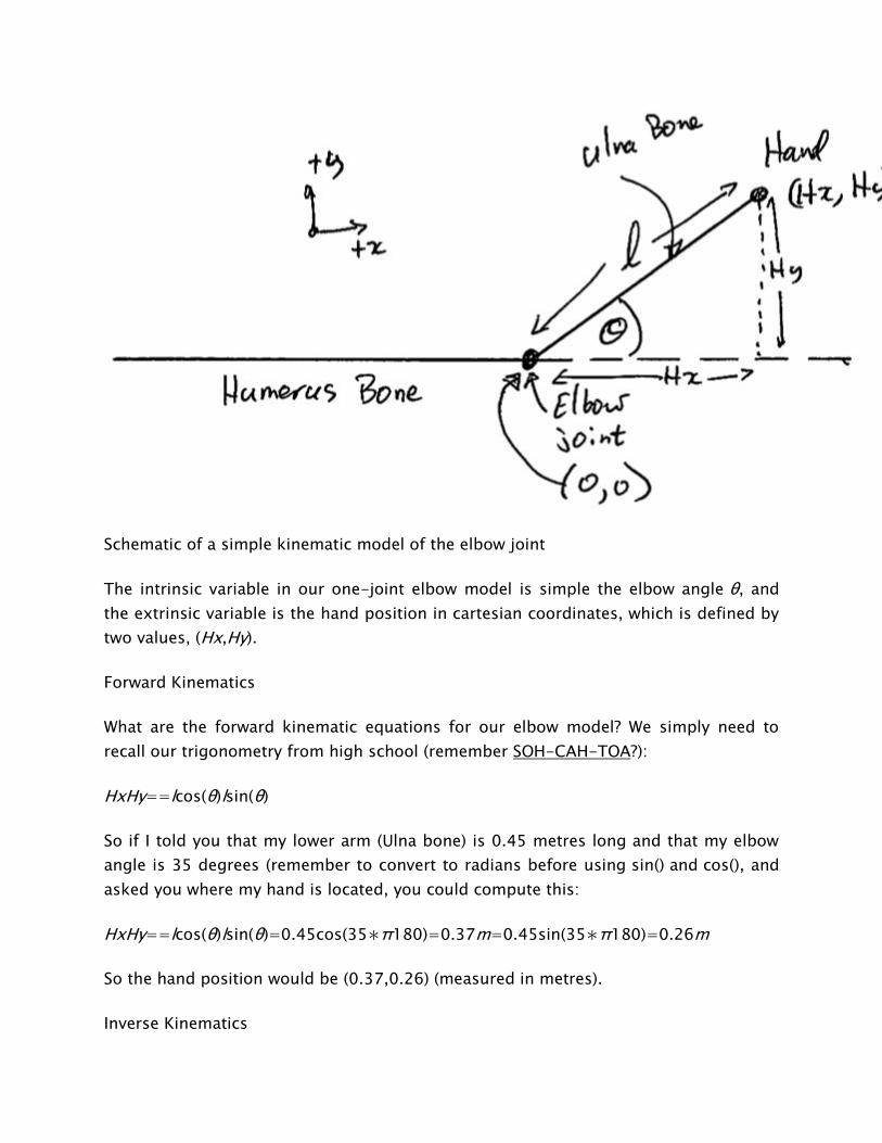
Page 2
Schematic of a simple kinematic model of the elbow joint
The intrinsic variable in our one-joint elbow model is simple the elbow angle θ, and
the extrinsic variable is the hand position in cartesian coordinates, which is defined by
two values, (Hx,Hy).
Forward Kinematics
What are the forward kinematic equations for our elbow model? We simply need to
recall our trigonometry from high school (remember SOH-CAH-TOA?):
HxHy==lcos(θ)lsin(θ)
So if I told you that my lower arm (Ulna bone) is 0.45 metres long and that my elbow
angle is 35 degrees (remember to convert to radians before using sin() and cos(), and
asked you where my hand is located, you could compute this:
HxHy==lcos(θ)lsin(θ)=0.45cos(35∗π180)=0.37m=0.45sin(35∗π180)=0.26m
So the hand position would be (0.37,0.26) (measured in metres).
Inverse Kinematics
Page 3
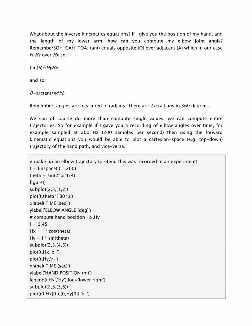
What about the inverse kinematics equations? If I give you the position of my hand, and
the length of my lower arm, how can you compute my elbow joint angle?
RememberSOH-CAH-TOA: tan() equals opposite (O) over adjacent (A) which in our case
is Hy over Hx so:
tan(θ)=HyHx
and so:
θ=arctan(HyHx)
Remember, angles are measured in radians. There are 2π radians in 360 degrees.
We can of course do more than compute single values, we can compute entire
trajectories. So for example if I gave you a recording of elbow angles over time, for
example sampled at 200 Hz (200 samples per second) then using the forward
kinematic equations you would be able to plot a cartesian-space (e.g. top-down)
trajectory of the hand path, and vice-versa.
# make up an elbow trajectory (pretend this was recorded in an experiment)
t = linspace(0,1,200)
theta = sin(2*pi*t/4)
figure()
subplot(2,3,(1,2))
plot(t,theta*180/pi)
xlabel('TIME (sec)')
ylabel('ELBOW ANGLE (deg)')
# compute hand position Hx,Hy
l = 0.45
Hx = l * cos(theta)
Hy = l * sin(theta)
subplot(2,3,(4,5))
plot(t,Hx,'b-')
plot(t,Hy,'r-')
xlabel('TIME (sec)')
ylabel('HAND POSITION (m)')
legend(('Hx','Hy'),loc='lower right')
subplot(2,3,(3,6))
plot((0,Hx[0]),(0,Hy[0]),'g-')
Page 4
plot((0,Hx[-1]),(0,Hy[-1]),'r-')
plot(Hx[0:-1:10],Hy[0:-1:10],'k.')
xlabel('X (m)')
ylabel('Y (m)')
axis('equal')
Example elbow movement
Two-joint arm
Let's introduce a shoulder joint as well:
Page 5
Schematic of a simple kinematic model of a two-joint arm
Forward Kinematics
Now let's think about the forward and inverse kinematic equations to go from intrinsic
coordinates, joint angles (θ1,θ2) to extrinsic coordinates (Hx,Hy). We will compute the
elbow joint position as an intermediate step.
ExEyHxHy====l1cos(θ1)l1sin(θ1)Ex+l2cos(θ1+θ2)Ey+l2sin(θ1+θ2)
Now if I give you a set of shoulder and elbow joint angles (θ1,θ2), you can compute
what my hand position (Hx,Hy) is.
We can visualize this mapping by doing something like the following: decide on a
range of shoulder angles and elbow angles that are physiologically realistic, and
sample that range equally in joint space … then run those joint angles through the
forward kinematics equations to visualize how those equally-spaced joint angles
correspond to cartesian hand positions.
# Function to transform joint angles (a1,a2) to hand position (Hx,Hy)
def joints_to_hand(a1,a2,l1,l2):
Ex = l1 * cos(a1)
Page 6
Ey = l1 * sin(a1)
Hx = Ex + (l2 * cos(a1+a2))
Hy = Ey + (l2 * sin(a1+a2))
return Ex,Ey,Hx,Hy
# limb geometry
l1 = 0.34 # metres
l2 = 0.46 # metres
# decide on a range of joint angles
n1steps = 10
n2steps = 10
a1range = linspace(0*pi/180, 120*pi/180, n1steps) # shoulder
a2range = linspace(0*pi/180, 120*pi/180, n2steps) # elbow
# sample all combinations and plot joint and hand coordinates
f=figure(figsize=(8,12))
for i in range(n1steps):
for j in range(n2steps):
subplot(2,1,1)
plot(a1range[i]*180/pi,a2range[j]*180/pi,'r+')
ex,ey,hx,hy = joints_to_hand(a1range[i], a2range[j], l1, l2)
subplot(2,1,2)
plot(hx, hy, 'r+')
subplot(2,1,1)
xlabel('Shoulder Angle (deg)')
ylabel('Elbow Angle (deg)')
title('Joint Space')
subplot(2,1,2)
xlabel('Hand Position X (m)')
ylabel('Hand Position Y (m)')
title('Hand Space')
a1 = a1range[n1steps/2]
a2 = a2range[n2steps/2]
ex,ey,hx,hy = joints_to_hand(a1,a2,l1,l2)
subplot(2,1,1)
plot(a1*180/pi,a2*180/pi,'bo',markersize=5)
Page 7
axis('equal')
xl = get(get(f,'axes')[0],'xlim')
yl = get(get(f,'axes')[0],'ylim')
plot((xl[0],xl[1]),(a2*180/pi,a2*180/pi),'b-')
plot((a1*180/pi,a1*180/pi),(yl[0],yl[1]),'b-')
subplot(2,1,2)
plot((0,ex,hx),(0,ey,hy),'b-')
plot(hx,hy,'bo',markersize=5)
axis('equal')
xl = get(get(f,'axes')[1],'xlim')
yl = get(get(f,'axes')[1],'ylim')
plot((xl[0],xl[1]),(hy,hy),'b-')
plot((hx,hx),(yl[0],yl[1]),'b-')
Page 9
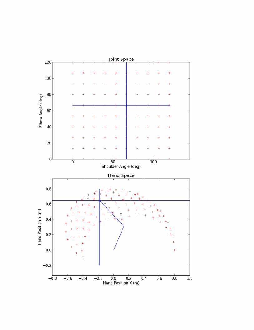
Joint vs Hand Kinematics for Two Joint Arm
Note that in the lower plot, the shoulder location is at the origin, (0,0). The blue
crosshairs in each subplot correspond to the same arm position — in joint space (top)
and in cartesian hand space (bottom).
We can note a few distinct features of this mapping between joint and hand space.
First, equal spacing across the workspace in joint space does not correspond to equal
spacing across the hand workspace, especially near the outer edges of the hand's
reach. Second, a square workspace region in joint space corresponds to a really curved
region in hand space. These complexities reflect the fact that the mapping between
joint space and hand space is non-linear.
Inverse Kinematics
You can start to appreciate the sorts of problems the brain must face when planning
arm movements. If I want move my hand through a particular hand path, what joint
angles does that correspond to? We must use inverse kinematics to determine this.
I will leave the inverse kinematics equations up to you to derive as one of the steps in
your assignment for this topic.
The Jacobian
So far we have looked at kinematic equations for arm positions — joint angular
positions and hand cartesian positions. Here we look at velocities (rate of change of
position) in the two coordinate frames, joint-space and hand-space.
How can we compute hand velocities dHdt given joint velocities dθdt? If we can we
compute an intermediate term dHdθ then we can apply the the Chain Rule:
dHdt=dHdθdθdt
This intermediate term is in fact known as the Jacobian (Wikipedia:Jacobian)
matrix J(θ) and is defined as:
J(θ)=dHdθ
and so:
Page 10
dHdt=J(θ)dθdt
Note that the Jacobian is written as J(θ) which means it is a function of joint angles θ —
in other words, the four terms in the Jacobian matrix (see below) change depending on
limb configuration (joint angles). This means the relationships between joint angles
and hand coordinates changes depending on where the limb is in its workspace. We
already have an idea that this is true, from the figure above.
For the sake of notational brevity we will refer to hand velocities as H˙ and joint
velocities as θ˙ and we will omit (from the notation) the functional dependence
of J on θ:
H˙=Jθ˙
The Jacobian is a matrix-valued function; you can think of it like a vector version of the
derivative of a scalar. The Jacobian matrix J encodes relationships between changes in
joint angles and changes in hand positions.
J=dHdθ=⎡⎣⎢⎢⎢∂Hx∂θ1,∂Hy∂θ1,∂Hx∂θ2∂Hy∂θ2⎤⎦⎥⎥⎥
For a system with 2 joint angles θ=(θ1,θ2) and 2 hand coordinates H=(Hx,Hy), the
Jacobian J is a 2x2 matrix where each value codes the rate of change of a given hand
coordinate with respect the given joint coordinate. So for example the
term ∂Hx∂θ2 represents the change in the x coordinate of the hand given a change in
the elbow joint angle θ2.
So how do we determine the four terms of J? We have to do calculus and differentiate
the equations for Hx and Hy with respect to the joint angles θ1 and θ2. Fortunately we
can use a Python package for symbolic computation called SymPy to help us with the
calculus. (you will have to install SymPy… on Ubuntu (or any Debian-based
GNU/Linux), just type sudo apt-get install python-sympy)
# import sympy
from sympy import *
# define these variables as symbolic (not numeric)
a1,a2,l1,l2 = symbols('a1 a2 l1 l2')
# forward kinematics for Hx and Hy
hx = l1*cos(a1) + l2*cos(a1+a2)
hy = l1*sin(a1) + l2*sin(a1+a2)
Page 11
# use sympy diff() to get partial derivatives for Jacobian matrix
J11 = diff(hx,a1)
J12 = diff(hx,a2)
J21 = diff(hy,a1)
J22 = diff(hy,a2)
print J11
print J12
print J21
print J22
In [12]: print J11
-l1*sin(a1) - l2*sin(a1 + a2)
In [13]: print J12
-l2*sin(a1 + a2)
In [14]: print J21
l1*cos(a1) + l2*cos(a1 + a2)
In [15]: print J22
l2*cos(a1 + a2)
So now we have the four terms of the Jacobian:
J=[−l1sin(θ1)−l2sin(θ1+θ2),l1cos(θ1)+l2cos(θ1+θ2),−l2sin(θ1+θ2)l2cos(θ1+θ2)]
and now we can write a Python function that returns the Jacobian, given a set of joint
angles:
def jacobian(A,aparams):
"""
Given joint angles A=(a1,a2)
returns the Jacobian matrix J(q) = dH/dA
"""
l1 = aparams['l1']
l2 = aparams['l2']
dHxdA1 = -l1*sin(A[0]) - l2*sin(A[0]+A[1])
dHxdA2 = -l2*sin(A[0]+A[1])
Page 12
dHydA1 = l1*cos(A[0]) + l2*cos(A[0]+A[1])
dHydA2 = l2*cos(A[0]+A[1])
J = matrix([[dHxdA1,dHxdA2],[dHydA1,dHydA2]])
return J
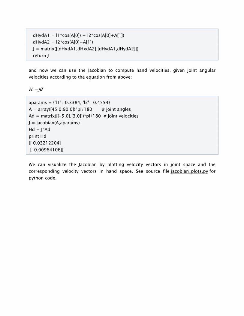
and now we can use the Jacobian to compute hand velocities, given joint angular
velocities according to the equation from above:
H˙=Jθ˙
aparams = {'l1' : 0.3384, 'l2' : 0.4554}
A = array([45.0,90.0])*pi/180 # joint angles
Ad = matrix([[-5.0],[3.0]])*pi/180 # joint velocities
J = jacobian(A,aparams)
Hd = J*Ad
print Hd
[[ 0.03212204]
[-0.00964106]]
We can visualize the Jacobian by plotting velocity vectors in joint space and the
corresponding velocity vectors in hand space. See source file jacobian_plots.py for
python code.
Page 13
Visualizing the Jacobian
Accelerations
We can also use the Jacobian to compute accelerations at the hand due to
accelerations at the joint, simply by differentiating our equations with respect to
time. Remember the equation for velocity:
H˙=Jθ˙
for acceleration we just differentiate both sides with respect to time:
H¨=ddt(H˙)=ddt(Jθ˙)
and apply the Product Rule from calculus:
Page 14
ddt(Jθ˙)=[J(ddtθ˙)]+[(ddtJ)θ˙]
simplifying further,
H¨=(J)(θ¨)+(J˙)(θ˙)
So if we have joint accelerations θ¨ and joint velocities θ˙, all we need is the
Jacobian J and the time derivative of the Jacobian J˙, and we can compute hand
accelerations H¨.
How do we get J˙? Again we can use SymPy, as above, and we get the following:
(I will just show the final Python function, not the SymPy part):
def jacobiand(A,Ad,aparams):
"""
Given joint angles A=(a1,a2) and velocities Ad=(a1d,a2d)
returns the time derivative of the Jacobian matrix d/dt (J)
"""
l1 = aparams['l1']
l2 = aparams['l2']
Jd11 = -l1*cos(A[0])*Ad[0] - l2*(Ad[0] + Ad[1])*cos(A[0] + A[1])
Jd12 = -l2*(Ad[0] + Ad[1])*cos(A[0] + A[1])
Jd21 = -l1*sin(A[0])*Ad[0] - l2*(Ad[0] + Ad[1])*sin(A[0] + A[1])
Jd22 = -l2*(Ad[0] + Ad[1])*sin(A[0] + A[1])
Jd = matrix([[Jd11, Jd12],[Jd21, Jd22]])
return Jd
Note that the time derivative of the Jacobian, J˙, is a function of both joint
angles θ and joint velocities θ˙.
Inverse Jacobian
We have seen how to compute hand velocities and accelerations given joint angles,
velocities and accelerations… but what about inverse kinematics? How do we compute
joint velocities given hand velocities? What about joint accelerations given hand
accelerations?
Recall for velocities that:
Page 15
Jθ˙=H˙
To solve for θ˙ we can simply multiply both sides of the equation by the matrix inverse
of the Jacobian:
θ˙=J−1H˙
In Numpy you can compute the inverse of a matrix using the inv() function.
Similarly for accelerations, we can do the following:
θ¨=J−1[H¨−((J˙)(θ˙))]
The Redundancy Problem
Notice something important (and unrealistic) about our simple two-joint arm model.
There is a one-to-one mapping between any two joint angles (θ1,θ2) and hand
position (Hx,Hy). That is to say, a given hand position is uniquely defined by a single
set of joint angles.
This is of course convenient for us in a model, and indeed many empirical paradigms
in sensory-motor neuroscience construct situations where this is true, so that it's easy
to go between intrinsic and extrinsic coordinate frames.
This is not how it is in the real musculoskeletal system, of course, where there is
a many-to-one mapping from intrinsic to extrinsic coordinates. The human arm has
not just two mechanical degrees of freedom (independent ways in which to move) but
seven. The shoulder is like a ball-socket joint, so it can rotate 3 ways (roll, pitch, yaw).
The elbow can rotate a single way (flexion/extension). The forearm, because of the
geometry of the radius and ulna bones, can rotate one way (pronation/supination), and
the wrist joint can rotate two ways (flexion/extension, and radial/ulnar deviation). This
is to say nothing about shoulder translation (the shoulder joint itself can be translated
up/down and fwd/back) and the many, many degrees of freedom of the fingers.
With 7 DOF at the joint level, and only three cartesian degrees of freedom at the hand
(the 3D position of the hand) we have 4 extra DOF. This means that there is a 4-
dimensional "null-space" where joint rotations within that 4D null space have no effect
on 3D hand position. Another way of putting this is, there are an infinite number of
ways of configuring the 7 joints of the arm to reach a single 3D hand position.
Page 16
How does the CNS choose to plan and control movements with all of this redundancy?
This is known in the sensory-motor neuroscience literature as the Redundancy
Problem.
Computational Models of Kinematics
The Minimum-Jerk Hypothesis
One of the early computational models of arm movement kinematics was described by
Tamar Flash and Neville Hogan. Tamar was a postdoc at MIT at the time, working with
Neville Hogan, a Professor there (as well as with Emilio Bizzi, another Professor at MIT).
Tamar is now a Professor at the Weizmann Institute of Science in Rehovot, Israel.
For a long time, researchers had noted striking regularities in the hand paths of multi-
joint arm movements. Movements were smooth, with unimodal, (mostly) symmetric
velocity profiles (so-called "bell-shaped" velocity profiles).
Morasso, P. (1981). Spatial control of arm movements. Experimental Brain
Research, 42(2), 223-227.
Soechting, J. F., & Lacquaniti, F. (1981). Invariant characteristics of a pointing
movement in man. The Journal of Neuroscience, 1(7), 710-720.
Abend, W., Bizzi, E., & Morasso, P. (1982). Human arm trajectory formation.
Brain: a journal of neurology, 105(Pt 2), 331.
Atkeson, C. G., & Hollerbach, J. M. (1985). Kinematic features of unrestrained
vertical arm movements. The Journal of Neuroscience, 5(9), 2318-2330.
Flash and Hogan investigated these patterns in the context of optimization theory — a
theory proposing that the brain plans and controls movements in an optimal way,
where optimal is defined by a specific task-related cost function. In other words, the
brain chooses movement paths and neural control signals that minimize some
objective cost function.
Todorov, E. (2004). Optimality principles in sensorimotor control. Nature
neuroscience, 7(9), 907-915.
Diedrichsen, J., Shadmehr, R., & Ivry, R. B. (2010). The coordination of
movement: optimal feedback control and beyond. Trends in cognitive sciences,
14(1), 31-39.
Page 17
Flash and Hogan wondered, at the kinematic level, what cost function might predict the
empirically observed patterns of arm movements?
They discovered that by minimizing the time integral of the square of "jerk", a simple
kinematic model predicted many of the regular patterns seen empirically for arm
movements of many kinds (moving from one point to another, or even moving through
via-points and moving around obstacles). Jerk is the rate of change (the derivative) of
acceleration, i.e. the second derivative of velocity, or the third derivative of position.
Essentially jerk is a measure of movement smoothness. Whether or not it turns out that
the brain is actually interested in minimizing jerk in order to plan and control arm
movements (an explanatory model), the minimum-jerk model turns out to be a good
descriptive model that is able to predict kinematics of multi-joint movement.
Hogan, N. (1984). An organizing principle for a class of voluntary movements.
The Journal of Neuroscience, 4(11), 2745-2754.
Flash, T. and Hogan, N. (1985) The coordination of arm movements: an
experimentally confirmed mathematical model. J. Neurosci. 7: 1688-1703.
Minimum Endpoint Variance
More recently, researchers have investigated how noise (variability) in neural control
signals affects movement kinematics. One hypothesis stemming from this work is that
the CNS plans and controls movements in such a way as to minimize the variance of
the endpoint (e.g. the hand, for a point-to-point arm movement). The idea is that the
effects of so-called "signal-dependent noise" in neural control signals accumulates
over the course of a movement, and so the hypothesis is that the CNS chooses specific
time-varying neural control signals that minimize the variability of the endpoint (e.g.
hand), for example at the final target location of a point-to-point movement.
Harris, C. M., & Wolpert, D. M. (1998). Signal-dependent noise determines
motor planning. Nature, 394(6695), 780-784.
van Beers, R. J., Haggard, P., & Wolpert, D. M. (2004). The role of execution
noise in movement variability. Journal of Neurophysiology, 91(2), 1050-1063.
Iguchi, N., Sakaguchi, Y., & Ishida, F. (2005). The minimum endpoint variance
trajectory depends on the profile of the signal-dependent noise. Biological
cybernetics, 92(4), 219-228.
Churchland, M. M., Afshar, A., & Shenoy, K. V. (2006). A central source of
movement variability. Neuron, 52(6), 1085-1096.
Page 18
Simmons, G., & Demiris, Y. (2006). Object grasping using the minimum variance
model. Biological cybernetics, 94(5), 393-407.
How does the brain plan and control movement?
Georgopoulos and colleagues in the 1980s recorded electrical activity of single motor
cortical neurons in awake, behaving monkeys during two-joint arm movemnets. The
general goal was to find out if patterns of neural activity could inform the question of
how the brain controls arm movements, and in particular, how large populations of
neurons might be coordinated to produce the patterns of arm movements empirically
observed.
Georgopoulos, A. P., Kalaska, J. F., Caminiti, R., & Massey, J. T. (1982). On the
relations between the direction of two-dimensional arm movements and cell
discharge in primate motor cortex. The Journal of Neuroscience, 2(11), 1527-
1537.
Georgopoulos, A. P., Caminiti, R., Kalaska, J. F., & Massey, J. T. (1983). Spatial
coding of movement: a hypothesis concerning the coding of movement direction
by motor cortical populations. Exp Brain Res Suppl, 7(32), 336.
Georgopoulos, A. P., Schwartz, A. B., & Kettner, R. E. (1986). Neuronal
population coding of movement direction. Science, 233(4771), 1416-1419.
Schwartz, A. B., Kettner, R. E., & Georgopoulos, A. P. (1988). Primate motor
cortex and free arm movements to visual targets in three-dimensional space. I.
Relations between single cell discharge and direction of movement. The Journal
of Neuroscience, 8(8), 2913-2927.
Georgopoulos, A. P., Kettner, R. E., & Schwartz, A. B. (1988). Primate motor
cortex and free arm movements to visual targets in three-dimensional space. II.
Coding of the direction of movement by a neuronal population. The Journal of
Neuroscience, 8(8), 2928-2937.
Kettner, R. E., Schwartz, A. B., & Georgopoulos, A. P. (1988). Primate motor
cortex and free arm movements to visual targets in three-dimensional space. III.
Positional gradients and population coding of movement direction from various
movement origins. The journal of Neuroscience, 8(8), 2938-2947.
Moran, D. W., & Schwartz, A. B. (1999). Motor cortical representation of speed
and direction during reaching. Journal of Neurophysiology, 82(5), 2676-2692.
An Alternate View
Page 19
A paper by Mussa-Ivaldi in 1988 showed that in fact the Georgopoulos finding that
broadly tuned neurons seem to encode hand movement kinematics does not imply that
the brain encodes kinematics… Mussa-Ivaldi showed that because in the motor system
so many kinematic and dynamic variables are correlated, broadly tuned neurons in
motor cortex could be shown to "encode" many intrinsic and extrinsic kinematic and
dynamic variables.
Mussa-Ivaldi, F. A. (1988). Do neurons in the motor cortex encode movement
direction? An alternative hypothesis. Neuroscience Letters, 91(1), 106-111.
Neural Prosthetics
The Georgopoulos results have been directly translated into the very applied problem
of using brain activity to control neural prosthetics, e.g. robotic prosthetic limbs. Form
a practical point of view, it may not matter how cortical neurons encode movement, as
long as we can build computational models (even just statistical models) of the
relationship between cortical activity and limb motion. Here are some examples.
Chapin, J. K., Moxon, K. A., Markowitz, R. S., & Nicolelis, M. A. (1999). Real-time
control of a robot arm using simultaneously recorded neurons in the motor
cortex. Nature neuroscience, 2, 664-670.
Taylor, D. M., Tillery, S. I. H., & Schwartz, A. B. (2002). Direct cortical control of
3D neuroprosthetic devices. Science, 296(5574), 1829-1832.
Donoghue, J. P. (2002). Connecting cortex to machines: recent advances in brain
interfaces. Nature Neuroscience, 5, 1085-1088.
Wolpaw, J. R., & McFarland, D. J. (2004). Control of a two-dimensional
movement signal by a noninvasive brain-computer interface in humans.
Proceedings of the National Academy of Sciences of the United States of
America, 101(51), 17849-17854.
Musallam, S., Corneil, B. D., Greger, B., Scherberger, H., & Andersen, R. A.
(2004). Cognitive control signals for neural prosthetics. Science, 305(5681),
258-262.
Hochberg, L. R., Serruya, M. D., Friehs, G. M., Mukand, J. A., Saleh, M., Caplan,
A. H., … & Donoghue, J. P. (2006). Neuronal ensemble control of prosthetic
devices by a human with tetraplegia. Nature, 442(7099), 164-171.
Santhanam, G., Ryu, S. I., Byron, M. Y., Afshar, A., & Shenoy, K. V. (2006). A
high-performance brain–computer interface. nature, 442(7099), 195-198.
Page 20
Velliste, M., Perel, S., Spalding, M. C., Whitford, A. S., & Schwartz, A. B. (2008).
Cortical control of a prosthetic arm for self-feeding. Nature, 453(7198), 1098-
1101.
Why are kinematic transformations important?
The many-to-one mapping issue is directly relevant to current key questions in
sensory-motor neuroscience. How does the nervous system choose a single arm
configuration when the goal is to place the hand at a specific 3D location in space? Of
course the redundancy problem as it's known, is not specific to kinematics. We have
many more muscles than joints, and so the problem crops up again: how does the CNS
choose a particular set of time-varying muscle forces, to produce a given set of joint
torques? The redundancy problem keeps getting worse as we go up the pipe: there
are many more neurons than muscles, and again, how does the CNS coordinate
millions of neurons to control orders-of-magnitude fewer muscles? These are key
questions that are still unresolved in modern sensory-motor neuroscience. Making
computational models where we can explicitly investigate these coordinate
transformations, and make predictions based on different proposed theories, is an
important way to address these kinds of questions.
Another category of scientific question where modeling kinematic transformations
comes in handy, is related to noise (I don't mean acoustic noise, i.e. loud noises, but
random variability). It is known that neural signals are "noisy". The many
transformations that sit in between neuronal control signals to muscles, and resulting
hand motion, are complex and nonlinear. How do noisy control signals manifest in
muscle forces, or joint angles, or hand positions? Are there predictable patterns of
variability in arm movement that can be attributed to these coordinate
transformations? If so, can we study how the CNS deals with this, i.e. compensates for
it (or not)?
This gives you a flavour for the sorts of questions one can begin to address, when you
have an explicit quantitative model of coordinate transformations. There are many
studies in arm movement control, eye movements, locomotion, etc, that use this basic
approach, combining experimental data with predictions from computational models.
Scott, S. H., and G. E. Loeb. "The computation of position sense from spindles in
mono-and multiarticular muscles." The Journal of neuroscience 14, no. 12
(1994): 7529-7540.
Page 21
Tweed, Douglas B., Thomas P. Haslwanter, Vera Happe, and Michael Fetter.
"Non-commutativity in the brain." Nature 399, no. 6733 (1999): 261-263.
Messier, J., & Kalaska, J. F. (1999). Comparison of variability of initial kinematics
and endpoints of reaching movements. Experimental Brain Research, 125(2),
139-152.
Loeb, E. P., S. F. Giszter, P. Saltiel and E. Bizzi, and F. A. Mussa-Ivaldi. "Output
units of motor behavior: an experimental and modeling study." Journal of
cognitive neuroscience 12, no. 1 (2000): 78-97.
Selen, Luc PJ, David W. Franklin, and Daniel M. Wolpert. "Impedance control
reduces instability that arises from motor noise." The Journal of Neuroscience
29, no. 40 (2009): 12606-12616.
Source:
http://www.gribblelab.org/compneuro2012/4_Computational_Motor_Control_Kinemati
cs.html


![KINEMATICS - new.excellencia.co.innew.excellencia.co.in/college/web/pdf/Kinematics-merged.pdf · KINEMATICS KINEMATICS WORKSHEET 1 1) Displacement is a _____ [ ] 1) Vector quantity](https://static.documents.pub/doc/80x56/5f356d4687229051801abace/kinematics-new-kinematics-kinematics-worksheet-1-1-displacement-is-a-.jpg)


