21
From Kinematics to Arm Control a)Calibrating the Kinematics Model b)Arm Motion Selection c)Motor Torque Calculations for a Planetary Robot Arm CS36510 1
| Date post: | 14-Dec-2015 |
| Category: |
Documents |
| Upload: | liliana-grymes |
| View: | 222 times |
| Download: | 1 times |
From Kinematics to Arm Control
a) Calibrating the Kinematics Model
b) Arm Motion Selection
c) Motor Torque Calculations for a Planetary Robot Arm
CS36510 1
a) Calibrating the Kinematics Model
• Resolution, Repeatability and Accuracy
• Causes of Mechanical Error
• Calibrating the kinematics model
CS36510 2
Resolution, Repeatability and Accuracy
1. Resolution: smallest incremental move that a robot can physically produce.
2. Repeatability: a measure of the robot’s ability to move back to the same position and orientation over and over again. Also referred to as ‘precision’.
3. Accuracy: the ability of the robot to move precisely to a desired position in 3D space
CS36510 3
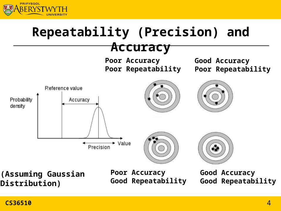
Repeatability (Precision) and Accuracy
Poor AccuracyPoor Repeatability
Good AccuracyPoor Repeatability
Poor AccuracyGood Repeatability
Good AccuracyGood Repeatability
(Assuming GaussianDistribution)
CS36510 4
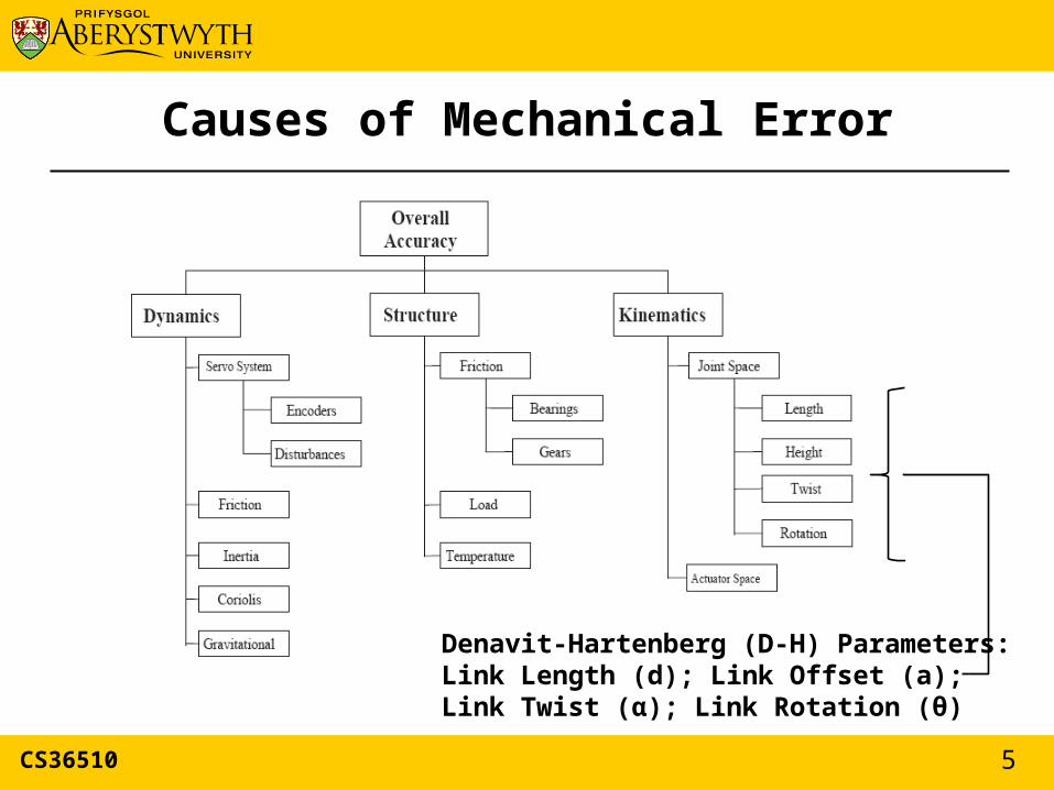
Causes of Mechanical Error
Denavit-Hartenberg (D-H) Parameters:Link Length (d); Link Offset (a); Link Twist (α); Link Rotation (θ)
CS36510 5
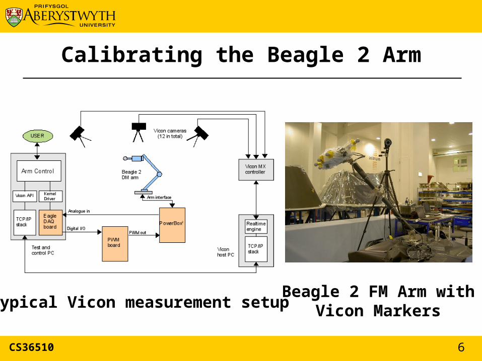
Calibrating the Beagle 2 Arm
Typical Vicon measurement setupBeagle 2 FM Arm with
Vicon Markers
CS36510 6
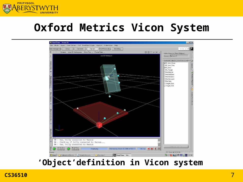
Oxford Metrics Vicon System
‘Object’definition in Vicon system
CS36510 7
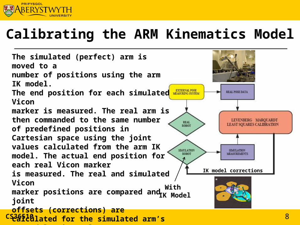
Calibrating the ARM Kinematics Model
The simulated (perfect) arm is moved to anumber of positions using the arm IK model. The end position for each simulated Viconmarker is measured. The real arm is then commanded to the same number of predefined positions in Cartesian space using the jointvalues calculated from the arm IK model. The actual end position for each real Vicon markeris measured. The real and simulated Viconmarker positions are compared and jointoffsets (corrections) are calculated for the simulated arm’s IK model using a least-squares fitting method.The result is that the simulated arm with the corrected IK model produces identicalpositioning results as the real arm. i.e. Thesimulated arm behaves as per the real arm.
CS36510
With IK Model
IK model corrections
8
b) Arm Motion Selection
• Joint-by-Joint Motion (JJM)
• Slew Motion (SM)
• Joint Interpolated Motion (JIM)
CS36510 9
Joint-by-Joint Motion (JJM or JBJ)
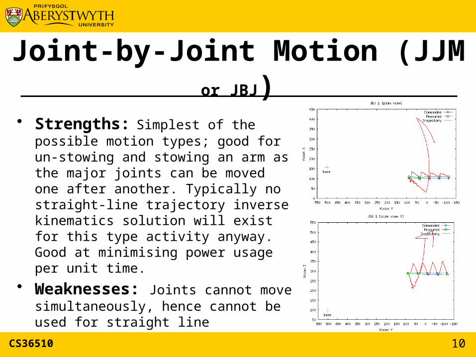
• Strengths: Simplest of the possible motion types; good for un-stowing and stowing an arm as the major joints can be moved one after another. Typically no straight-line trajectory inverse kinematics solution will exist for this type activity anyway. Good at minimising power usage per unit time.
• Weaknesses: Joints cannot move simultaneously, hence cannot be used for straight line (continuous) trajectories. Rather payload motion will be in an series of arcs. Large total time to complete all joint motions.
CS36510 10
Slew Motion (SM)
CS36510 11
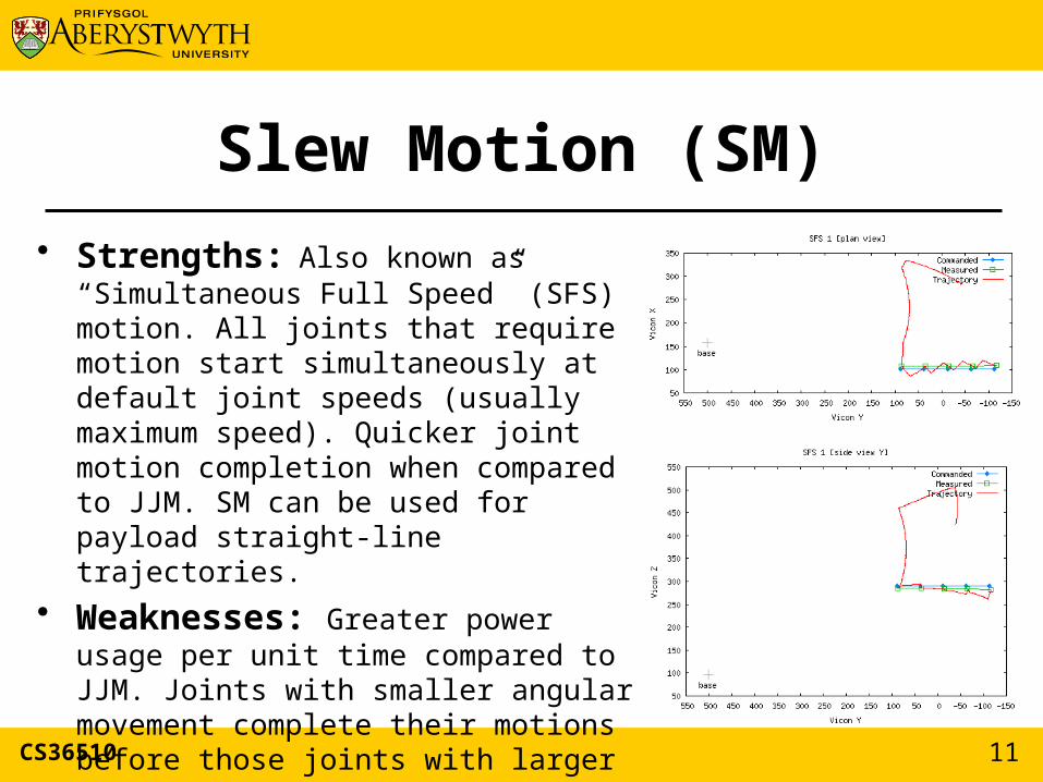
• Strengths: Also known as “Simultaneous Full Speed” (SFS) motion. All joints that require motion start simultaneously at default joint speeds (usually maximum speed). Quicker joint motion completion when compared to JJM. SM can be used for payload straight-line trajectories.
• Weaknesses: Greater power usage per unit time compared to JJM. Joints with smaller angular movement complete their motions before those joints with larger angular movements. Smooth straight-line trajectories not possible. Payload motion tends to zig-zag about the desired straight-line trajectory.
Joint Interpolated Motion (JIM)
CS36510 12
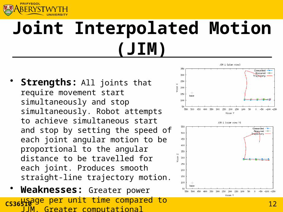
• Strengths: All joints that require movement start simultaneously and stop simultaneously. Robot attempts to achieve simultaneous start and stop by setting the speed of each joint angular motion to be proportional to the angular distance to be travelled for each joint. Produces smooth straight-line trajectory motion.
• Weaknesses: Greater power usage per unit time compared to JJM. Greater computational overheads when compared to SM.
Knot Points
CS36510 13
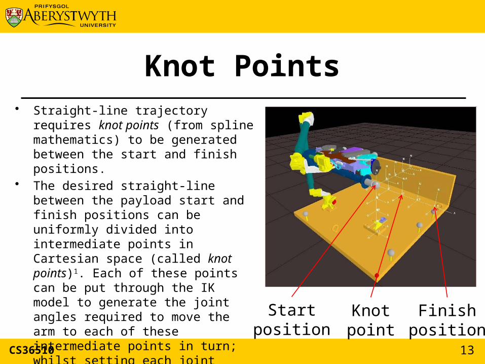
• Straight-line trajectory requires knot points (from spline mathematics) to be generated between the start and finish positions.
• The desired straight-line between the payload start and finish positions can be uniformly divided into intermediate points in Cartesian space (called knot points)1. Each of these points can be put through the IK model to generate the joint angles required to move the arm to each of these intermediate points in turn; whilst setting each joint speed (e.g. proportional for JIM) to the required angular motion.
1 Taylor, R. H., Planning and Execution of Straight Line Manipulator
Trajectories, IBM J. RES. DEVELOP, VOL. 23, NO. 4, pp. 424-436,
JULY 1979.
Startposition
Finishposition
Knotpoint
c) Motor Torque Calculations for aPlanetary Robot Arm
• What is torque, and why do we need it?– Torque (τ) is defined as a turning (or twisting)
force– A robot arm joint motor, with an attached
linkage and payload, has to generate a torque to be able to move the linkage and payload
– The magnitude of τ depends upon the payload force, and the length of the joint motor linkage
CS36510 14
Torque Equation - 1
CS36510 15
τ = F × lwhere τ is the magnitude of the torque (N·m), l (in meters) is the linkage length, and F (in Newtons)is the magnitude of the force.
In the vertical plane, the force acting upon an object (causingit to fall) is the acceleration due to gravity (for Earth, g ≈ 9.81 m/sec2).
Therefore F = m × g, where m is the magnitude of the mass of theobject (in kg), and F is normally referred to as the object’s weight.
CS36510 16
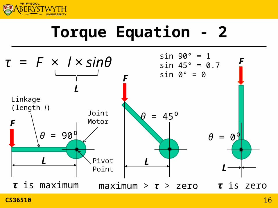
Torque Equation - 2
Fθ = 90⁰
F
θ = 45⁰
F
θ = 0⁰
τ is zeroτ is maximum
sin 90° = 1sin 45° = 0.7sin 0° = 0
τ = F × l × sinθ
L
L LL
JointMotor
Linkage(length l)
maximum > τ > zero
PivotPoint
CS36510 17
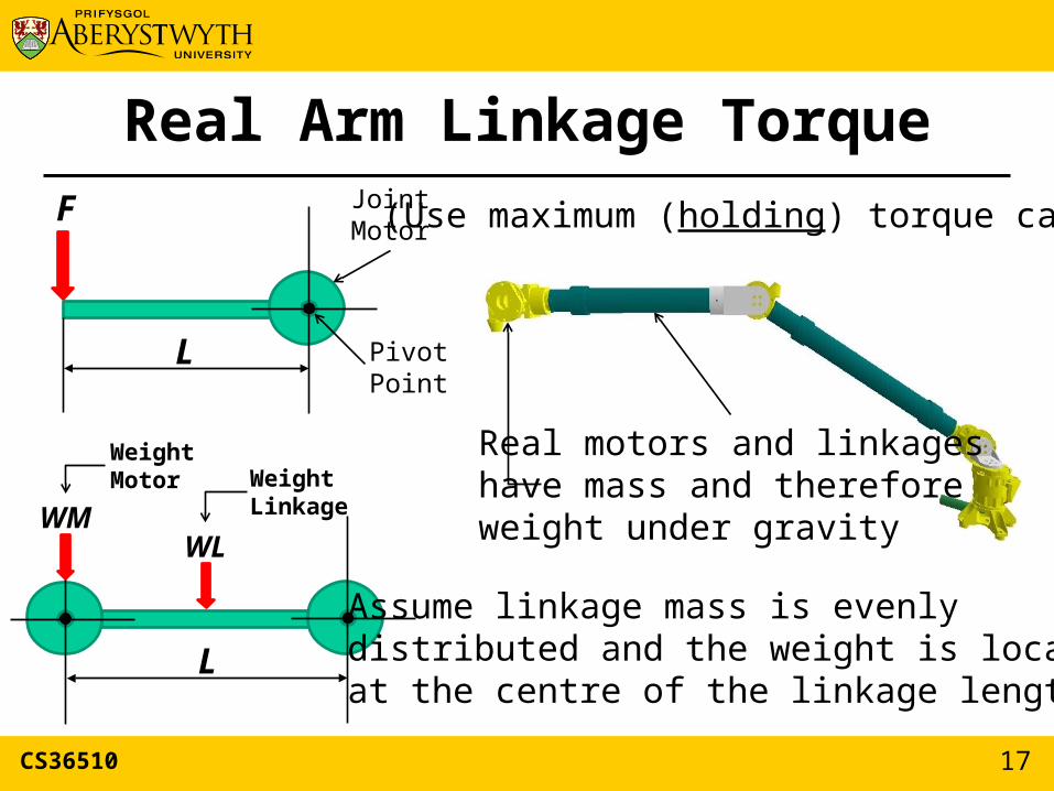
Real Arm Linkage TorqueF
L
JointMotor
PivotPoint
(Use maximum (holding) torque case)
L
WLWM
Real motors and linkageshave mass and thereforeweight under gravity
Assume linkage mass is evenlydistributed and the weight is located at the centre of the linkage length
WeightMotor Weight
Linkage
CS36510 18
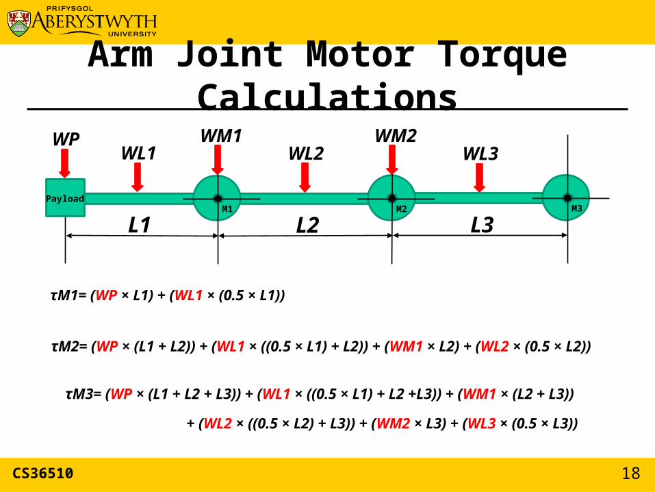
Arm Joint Motor Torque Calculations
L3L2L1
WPWL1 WL2 WL3
WM1 WM2
τM1= (WP × L1) + (WL1 × (0.5 × L1))
τM2= (WP × (L1 + L2)) + (WL1 × ((0.5 × L1) + L2)) + (WM1 × L2) + (WL2 × (0.5 × L2))
τM3= (WP × (L1 + L2 + L3)) + (WL1 × ((0.5 × L1) + L2 +L3)) + (WM1 × (L2 + L3))
+ (WL2 × ((0.5 × L2) + L3)) + (WM2 × L3) + (WL3 × (0.5 × L3))
PayloadM1 M2 M3
CS36510 19
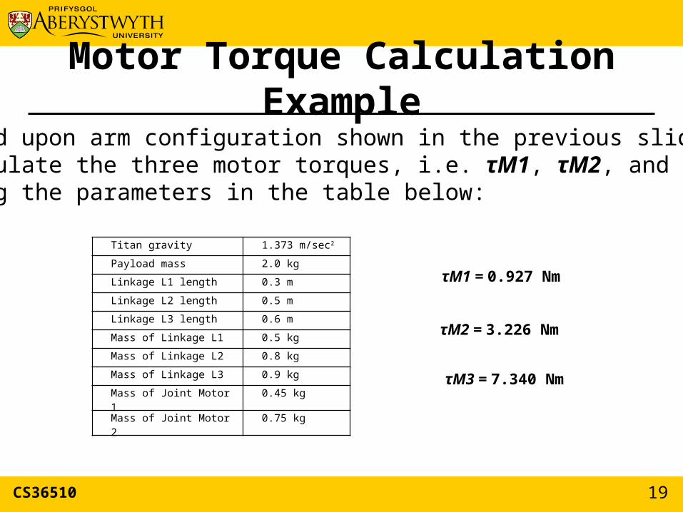
Motor Torque Calculation Example
τM1 = 0.927 Nm
τM2 = 3.226 Nm
τM3 = 7.340 Nm
Titan gravity 1.373 m/sec2
Payload mass 2.0 kg
Linkage L1 length 0.3 m
Linkage L2 length 0.5 m
Linkage L3 length 0.6 m
Mass of Linkage L1 0.5 kg
Mass of Linkage L2 0.8 kg
Mass of Linkage L3 0.9 kg
Mass of Joint Motor 1 0.45 kg
Mass of Joint Motor 2 0.75 kg
Based upon arm configuration shown in the previous slide,calculate the three motor torques, i.e. τM1, τM2, and τM3,using the parameters in the table below:

Gear Box Selection:
a) A gear box will be needed to achieved desired output motor torque
b) Gear Box Torque Ratio is ratio of output torque to input torque, e.g. 100:1, 1000:1 etc.
c) E.g. for τM3 select 73.1 × 10-3 Nm × 100:1 = 7.31 Nm
CS36510 20
Final Points
• Maximum holding torques calculated for each motor. Would need to add contingency (e.g. 20%) for each motor.
• Calibration, motion selection, and motor torques also apply to a rover locomotion chassis, i.e. steering and drive mechanism
• Same techniques can be applied, but chassis details not covered here
CS36510 21


