284

2
Computer Simulation Studies
of Minerals
Artem Romaevich Oganov
University College London
Thesis submitted in fulfilment of the requirements
for the degree of Doctor of Philosophy
to the
University of London
2002
3
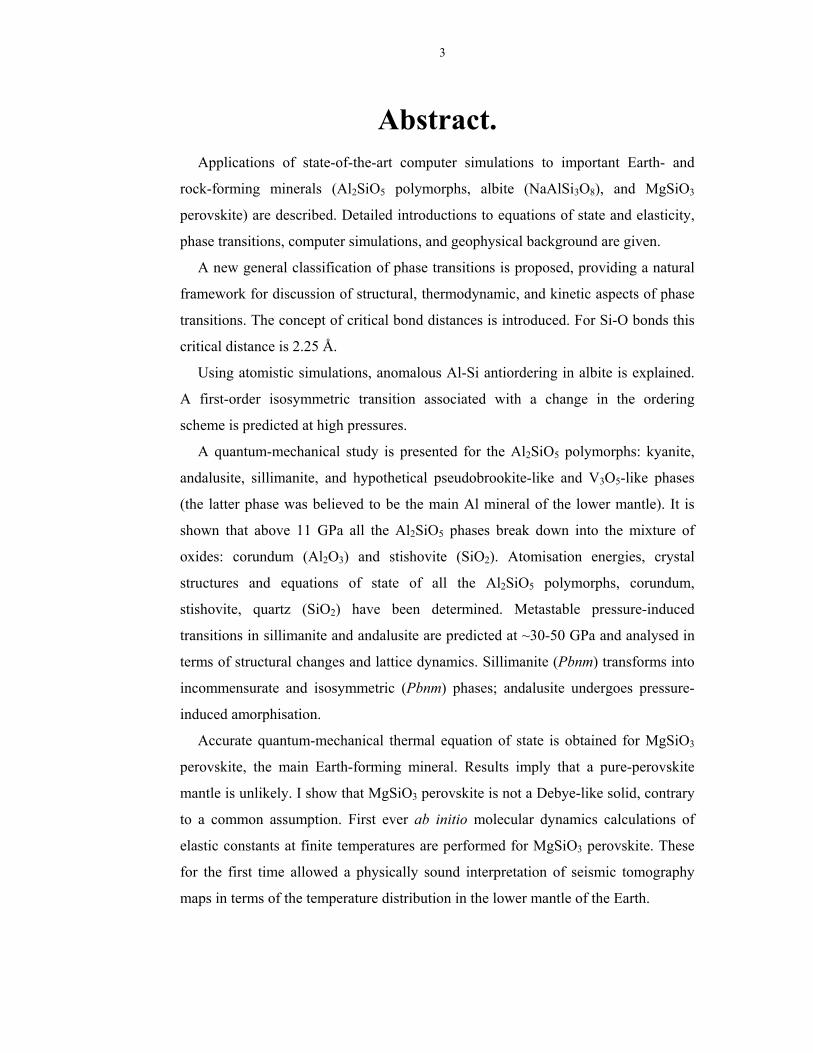
Abstract. Applications of state-of-the-art computer simulations to important Earth- and
rock-forming minerals (Al2SiO5 polymorphs, albite (NaAlSi3O8), and MgSiO3
perovskite) are described. Detailed introductions to equations of state and elasticity,
phase transitions, computer simulations, and geophysical background are given.
A new general classification of phase transitions is proposed, providing a natural
framework for discussion of structural, thermodynamic, and kinetic aspects of phase
transitions. The concept of critical bond distances is introduced. For Si-O bonds this
critical distance is 2.25 Å.
Using atomistic simulations, anomalous Al-Si antiordering in albite is explained.
A first-order isosymmetric transition associated with a change in the ordering
scheme is predicted at high pressures.
A quantum-mechanical study is presented for the Al2SiO5 polymorphs: kyanite,
andalusite, sillimanite, and hypothetical pseudobrookite-like and V3O5-like phases
(the latter phase was believed to be the main Al mineral of the lower mantle). It is
shown that above 11 GPa all the Al2SiO5 phases break down into the mixture of
oxides: corundum (Al2O3) and stishovite (SiO2). Atomisation energies, crystal
structures and equations of state of all the Al2SiO5 polymorphs, corundum,
stishovite, quartz (SiO2) have been determined. Metastable pressure-induced
transitions in sillimanite and andalusite are predicted at ~30-50 GPa and analysed in
terms of structural changes and lattice dynamics. Sillimanite (Pbnm) transforms into
incommensurate and isosymmetric (Pbnm) phases; andalusite undergoes pressure-
induced amorphisation.
Accurate quantum-mechanical thermal equation of state is obtained for MgSiO3
perovskite, the main Earth-forming mineral. Results imply that a pure-perovskite
mantle is unlikely. I show that MgSiO3 perovskite is not a Debye-like solid, contrary
to a common assumption. First ever ab initio molecular dynamics calculations of
elastic constants at finite temperatures are performed for MgSiO3 perovskite. These
for the first time allowed a physically sound interpretation of seismic tomography
maps in terms of the temperature distribution in the lower mantle of the Earth.

4
To my brother for his wedding;
To my mother for the wedding of her son.
Acknowledgements. I am very grateful to the Russian President Scholarship for Education Abroad,
UCL Graduate School Research Scholarship, and the Overseas Research Scholarship
of the UK Government for the support of my studies at UCL.
My supervisors, J.P. Brodholt and G.D. Price, have provided me with their
supervision, support, and encouragement throughout my PhD course. They have
made my PhD experience very enjoyable, and I am much indebted to them for this
and for the many scientific discussions that we had. The whole Department of
Geological Sciences of UCL proved to be a very inspiring scientific community,
where I had learnt much from D. Alfé, L. Vočadlo, and I. Wood. I am grateful to my
colleagues in the Department of Physics and Astronomy – especially M. Gillan, J.
Harding, L. Kantorovich, J. Gavartin. For inspiring discussions I thank M. Catti
(Milano), J. Gale (Imperial College London), G. Kresse (Vienna), P. Ballone
(Messina), B. Karki (Minneapolis), H. Barron (Bristol), P. Dorogokupets (Irkutsk),
O. Kuskov and V. Polyakov (Moscow), M. Hostettler (Lausanne), T. Balič-Zunič
(Copenhagen), R. Angel (Blacksburg), and many others.
My teachers - T. Shakhova, B. Glybin, M. Maryashin, N. Cherkasskaya, G.
Litvinskaya, V. Urusov, and D. Pushcharovsky - have formed my scientific interests
and skills. I am infinitely grateful to my mother Galina for everything; my uncle
Felix has always remained for me an example. I am indeed very fortunate to have
met so many remarkable people in my life.

5
Contents. Abstract 2
Acknowledgements 3
Contents 4
List of figures and tables 8
CHAPTER 1. INTRODUCTION 12
CHAPTER 2. EARTH’S MODELS 14
2.1. Overview 14
2.2. Origin and energetics of the Earth 15
2.3. Elemental abundances 17
2.4. Geophysical observations: stratification of the Earth 19
2.5. PREM and other spherical models 22
2.6. Interpretation of PREM: composition and temperature 25
2.7. The Dynamic Earth: plate tectonics and convection 31
2.8. Seismic tomography and mantle dynamics 34
CHAPTER 3. THERMODYNAMICS, EQUATIONS OF STATE,
AND ELASTICITY OF CRYSTALS
41
3.1. Thermodynamic properties of crystals 41
3.2. Harmonic approximation 42
3.3. Models of the phonon spectrum: Debye, Agoshkov, Kieffer 44
3.4. Shortcomings of the harmonic approximation 47
3.5. Quasiharmonic approximation (QHA) 49
3.6. Beyond the QHA: intrinsic anharmonicity 50
3.7. Equation of state (EOS) – general thermodynamic
formulation
52
3.8. Analytical representations of the equation of state 56
3.9. EOS, internal strain, and phase transitions 63
3.10. Elastic constants 66

6
3.11. Cauchy relations 72
3.12. Mechanical stability 73
3.13. Birch’s law and effects of temperature on elastic
constants
74
CHAPTER 4. PHASE TRANSITIONS 76
4.1. Classifications of phase transitions 76
4.2. Theoretical framework 78
4.2.1. First-order phase transitions 78
4.2.2. Landau theory of first-and second-order transitions 80
4.2.3. Renormalisation group theory (RGT) 85
4.2.4. Ising spin model 87
4.2.5. Mean-field treatment of order-disorder phenomena 90
4.3. New classification of phase transitions 91
4.3.1. Phase transition scenarios 91
4.3.2. New classification 93
4.3.3. Phenomenology and examples of local phase
transitions
97
4.3.3.1. Isosymmetric transitions 97
4.4.3.2. Transitions with group-subgroup relations 101
4.4.3.3. Incommensurate transitions 102
4.4.3.4. Crystal-quasicrystal transitions 102
4.4.3.5. Pressure-induced amorphisation 103
4.4. Discussion of the new classification 106
CHAPTER 5. SIMULATION METHODS 108
5.1. An essay on the state of the art of predictive crystal
chemistry
108
5.1.1. Modern theoretical and predictive crystal
chemistry
109
5.2. Formulation of the general problem and the Born-
Oppenheimer principle
110
5.3. Methods of calculating the internal energy 112
5.3.1. Hartree method 114
5.3.2. Hartree-Fock method 116
5.3.3. Density functional theory (DFT) – introduction 120
7
5.3.4. Density functional theory (DFT) – approximate
functionals
129
5.3.5. Technical details of ab initio simulations 138
5.3.6. Semiclassical simulations 147
5.4. Lattice dynamics (LD) 155
5.5. Molecular dynamics (MD) 159
CHAPTER 6. ANTIORDERING IN ALBITE (NAALSI3O8) 165
6.1. Introduction 165
6.2. Computer simulations 168
6.3. Results 170
6.4. Nature of the antiordering 173
6.5. Hartree-Fock calculations: correlation of Na position and
Al-Si ordering in albite
174
CHAPTER 7. IONIC MODELLING OF AL2SIO5 POLYMORPHS 176
7.1. Introduction 176
7.2. Mineralogy of Al in the lower mantle 178
7.3. Simulation results 180
CHAPTER 8. HIGH-PRESSURE STABILITY OF AL2SIO5 AND
MINERALOGY OF ALUMINIUM IN THE EARTH'S LOWER
MANTLE: AB INITIO CALCULATIONS.
184
8.1. Computational methodology 184
8.2. Results 187
8.3. Discussion 192
CHAPTER 9. METASTABLE AL2SIO5 POLYMORPHS 198
9.1. Introduction 198
9.2. Computational methodology 199
9.3. Accuracy of simulations 200
9.5. Phase transitions in sillimanite 201
9.6. Phase transitions in andalusite 208
9-7. Discussion and conclusions 210
CHAPTER 10. THERMOELASTICITY AND PHASE
TRANSITIONS OF MGSIO3 PEROVSKITE
213
10.1. Introduction 213
10.2. Computational methodology 215
8
10.3. Comparative study of LD, MD and Debye model
applied to MgSiO3 perovskite
222
10.4. Stability of MgSiO3 perovskite 229
10.5. Equation of state and mantle geotherm 235
10.6. Elastic constants at mantle temperatures and pressures 241
10.7. Interpretation of seismic tomography 242
CHAPTER 11. CONCLUSIONS 247
REFERENCES 248
Appendix A: List of publications 281
Appendix B: Published papers (attached separately)
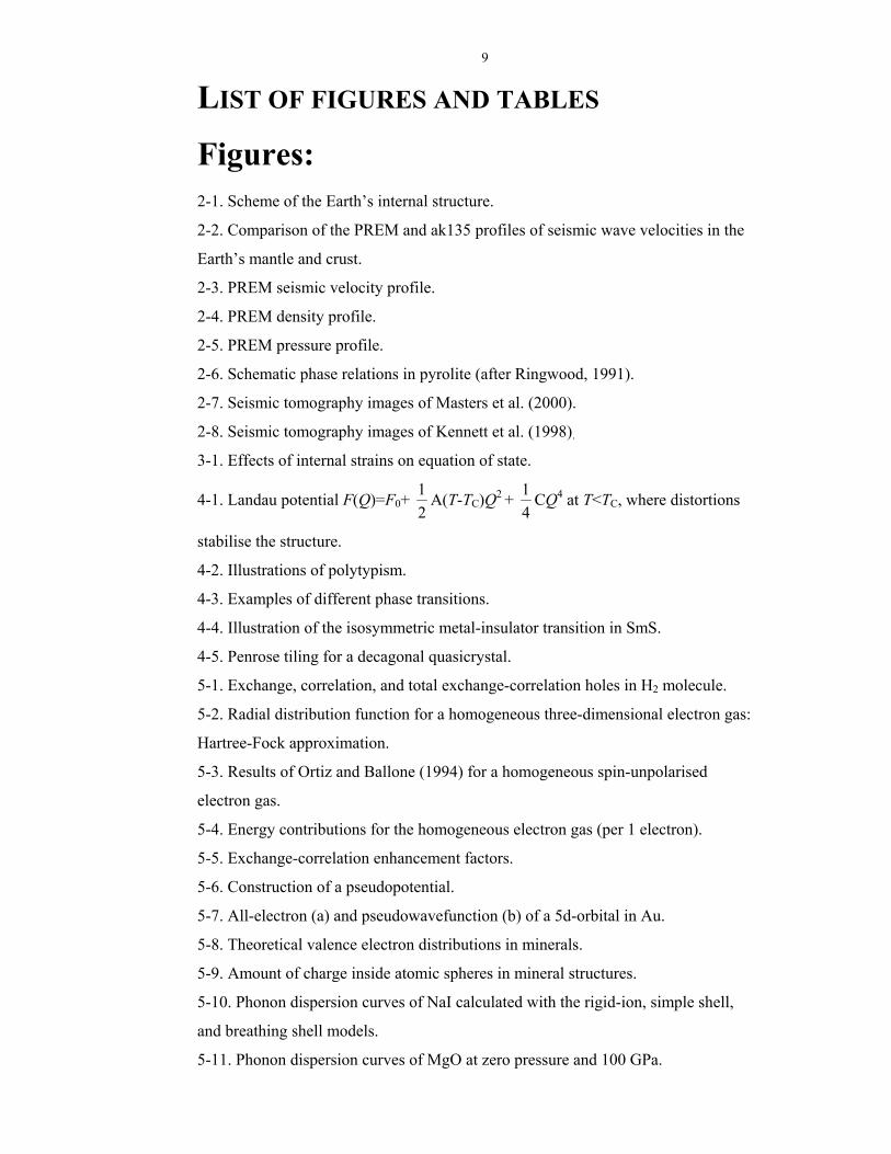
9
LIST OF FIGURES AND TABLES
Figures: 2-1. Scheme of the Earth’s internal structure.
2-2. Comparison of the PREM and ak135 profiles of seismic wave velocities in the
Earth’s mantle and crust.
2-3. PREM seismic velocity profile.
2-4. PREM density profile.
2-5. PREM pressure profile.
2-6. Schematic phase relations in pyrolite (after Ringwood, 1991).
2-7. Seismic tomography images of Masters et al. (2000).
2-8. Seismic tomography images of Kennett et al. (1998).
3-1. Effects of internal strains on equation of state.
4-1. Landau potential F(Q)=F0+ 21 A(T-TC)Q2 +
41 CQ4 at T<TC, where distortions
stabilise the structure.
4-2. Illustrations of polytypism.
4-3. Examples of different phase transitions.
4-4. Illustration of the isosymmetric metal-insulator transition in SmS.
4-5. Penrose tiling for a decagonal quasicrystal.
5-1. Exchange, correlation, and total exchange-correlation holes in H2 molecule.
5-2. Radial distribution function for a homogeneous three-dimensional electron gas:
Hartree-Fock approximation.
5-3. Results of Ortiz and Ballone (1994) for a homogeneous spin-unpolarised
electron gas.
5-4. Energy contributions for the homogeneous electron gas (per 1 electron).
5-5. Exchange-correlation enhancement factors.
5-6. Construction of a pseudopotential.
5-7. All-electron (a) and pseudowavefunction (b) of a 5d-orbital in Au.
5-8. Theoretical valence electron distributions in minerals.
5-9. Amount of charge inside atomic spheres in mineral structures.
5-10. Phonon dispersion curves of NaI calculated with the rigid-ion, simple shell,
and breathing shell models.
5-11. Phonon dispersion curves of MgO at zero pressure and 100 GPa.
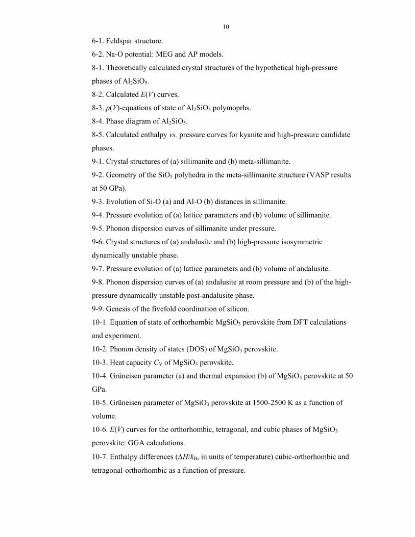
10
6-1. Feldspar structure.
6-2. Na-O potential: MEG and AP models.
8-1. Theoretically calculated crystal structures of the hypothetical high-pressure
phases of Al2SiO5.
8-2. Calculated E(V) curves.
8-3. p(V)-equations of state of Al2SiO5 polymoprhs.
8-4. Phase diagram of Al2SiO5.
8-5. Calculated enthalpy vs. pressure curves for kyanite and high-pressure candidate
phases.
9-1. Crystal structures of (a) sillimanite and (b) meta-sillimanite.
9-2. Geometry of the SiO5 polyhedra in the meta-sillimanite structure (VASP results
at 50 GPa).
9-3. Evolution of Si-O (a) and Al-O (b) distances in sillimanite.
9-4. Pressure evolution of (a) lattice parameters and (b) volume of sillimanite.
9-5. Phonon dispersion curves of sillimanite under pressure.
9-6. Crystal structures of (a) andalusite and (b) high-pressure isosymmetric
dynamically unstable phase.
9-7. Pressure evolution of (a) lattice parameters and (b) volume of andalusite.
9-8. Phonon dispersion curves of (a) andalusite at room pressure and (b) of the high-
pressure dynamically unstable post-andalusite phase.
9-9. Genesis of the fivefold coordination of silicon.
10-1. Equation of state of orthorhombic MgSiO3 perovskite from DFT calculations
and experiment.
10-2. Phonon density of states (DOS) of MgSiO3 perovskite.
10-3. Heat capacity CV of MgSiO3 perovskite. 10-4. Grüneisen parameter (a) and thermal expansion (b) of MgSiO3 perovskite at 50
GPa.
10-5. Grüneisen parameter of MgSiO3 perovskite at 1500-2500 K as a function of
volume.
10-6. E(V) curves for the orthorhombic, tetragonal, and cubic phases of MgSiO3
perovskite: GGA calculations.
10-7. Enthalpy differences (∆H/kB, in units of temperature) cubic-orthorhombic and
tetragonal-orthorhombic as a function of pressure.
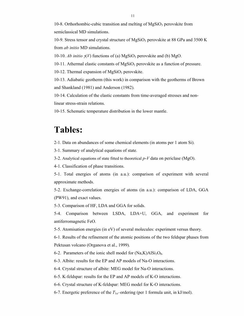
11
10-8. Orthorhombic-cubic transition and melting of MgSiO3 perovskite from
semiclassical MD simulations.
10-9. Stress tensor and crystal structure of MgSiO3 perovskite at 88 GPa and 3500 K
from ab initio MD simulations.
10-10. Ab initio γ(V) functions of (a) MgSiO3 perovskite and (b) MgO.
10-11. Athermal elastic constants of MgSiO3 perovskite as a function of pressure.
10-12. Thermal expansion of MgSiO3 perovskite.
10-13. Adiabatic geotherm (this work) in comparison with the geotherms of Brown
and Shankland (1981) and Anderson (1982).
10-14. Calculation of the elastic constants from time-averaged stresses and non-
linear stress-strain relations.
10-15. Schematic temperature distribution in the lower mantle.
Tables: 2-1. Data on abundances of some chemical elements (in atoms per 1 atom Si).
3-1. Summary of analytical equations of state.
3-2. Analytical equations of state fitted to theoretical p-V data on periclase (MgO).
4-1. Classification of phase transitions.
5-1. Total energies of atoms (in a.u.): comparison of experiment with several
approximate methods.
5-2. Exchange-correlation energies of atoms (in a.u.): comparison of LDA, GGA
(PW91), and exact values.
5-3. Comparison of HF, LDA and GGA for solids.
5-4. Comparison between LSDA, LDA+U, GGA, and experiment for
antiferromagnetic FeO.
5-5. Atomisation energies (in eV) of several molecules: experiment versus theory.
6-1. Results of the refinement of the atomic positions of the two feldspar phases from
Pektusan volcano (Organova et al., 1999).
6-2. Parameters of the ionic shell model for (Na,K)AlSi3O8.
6-3. Albite: results for the EP and AP models of Na-O interactions.
6-4. Crystal structure of albite: MEG model for Na-O interactions.
6-5. K-feldspar: results for the EP and AP models of K-O interactions.
6-6. Crystal structure of K-feldspar: MEG model for K-O interactions.
6-7. Energetic preference of the T1o–ordering (per 1 formula unit, in kJ/mol).

12
6-8. Mulliken charges and total energy of albite from Hartree-Fock calculations
(STO-3G basis).
7-1. Parameters of the ionic shell model for Al2SiO5.
7-2. Crystal structure of sillimanite.
7-3. Elastic properties of andalusite and sillimanite: experiment (Vaughan &
Weidner, 1978) and ionic model.
7-4. Ionic model predictions for the hypothetical high-pressure phases of Al2SiO5.
8-1. Phases in Al2O3-SiO2 system: theoretical results and experimental data.
8-2. The energy and volume effects of mineral transformations at zero pressure:
theory and experiment.
9-1. Crystal structure and equation of state of the meta-sillimanite phase.
9-2. Geometry of the SiO5 polyhedra.
10-1. Ab initio simulations of MgSiO3 perovskite.
10-2. Performance of the fitted interatomic potential: crystal structure and elastic
properties of MgSiO3 perovskite.
10-3. EOS of MgSiO3 perovskite from semiclassical calculations.
10-4. Elastic properties of MgSiO3 perovskite as a function of pressure (at 298 K).
10-5. Ab initio thermal EOS of MgSiO3 perovskite.
10-6. Thermoelastic parameters of MgSiO3 perovskite from theory and experiment.
10-7. Elastic properties of MgSiO3 perovskite at high pressures and temperatures.
13
Chapter 1. Introduction. Quantum-mechanical and atomistic simulations play an increasingly important
role in understanding the behaviour and properties of materials. On one hand, such
simulations provide a detailed microscopic picture of condensed-matter phenomena
(phase transitions, atomic motion and diffusion), which is difficult or impossible to
obtain experimentally. On the other hand, macroscopic properties (thermodynamics,
elasticity, equation of state, phase diagram) can be calculated and linked to the
microscopic picture and, in case of Earth- and planet-forming materials, to the global
planetary processes.
The main objective of this thesis is to show how solid state physics and computer
simulations of materials can be applied to geological problems. Enormous progress
has been made in this field since 1980-s; many important results in this field were
obtained at UCL, and some of the most recent major results will be discussed in this
thesis. Both theoretical background and examples from my recent works are
presented.
The first four chapters, ‘Earth’s models’, ‘Thermoelastic properties’, ‘Simulation
methods’, and ‘Phase transitions’ are largely introductory and contain most of the
theoretical background and equations used in later chapters, which will be dedicated
to particular systems of interest. Much of this theory can be found in well-known
books and reviews, but some was developed by myself. References to the original or
review literature are given throughout, although often (especially when the original
publications were too old) I preferred to cite later reviews or books that can be
consulted on each particular topic.
Subsequent chapters deal with results obtained for several particular mineral
systems, including albite (NaAlSi3O8), the Al2SiO5 polymorphs, and MgSiO3
perovskite. Both geological and physical implications of the results are
discussed. Most of the results presented here have been published
and extensively presented at a number of conferences and research
seminars. Appendix gives a list of these publications and presentations.
Chapter 11 gives some concluding remarks and outlines directions of
future work. Some parts of this thesis (especially in Chapters 3, 4, 5,
and 7) were taken from my MSc thesis (1997, University of Moscow), often with
only few changes.

14
A number of abbreviations have been introduced and used in many parts of this
thesis. For convenience, here I list some of them:
BM – Birch-Murnaghan equation of state (BM2 – 2nd-order, BM3 – 3rd-order)
DFT – Density Functional Theory
DM – Debye Model
DOS – Density Of States
EOS – Equation Of State
GEA – Gradient Expansion Approximation
GGA – Generalised Gradient Approximation
HF – Hartree-Fock approximation
LAPW – Linearised Augmented Plane Wave method
LCAO – Linear Combination of Atomic Orbitals
LD – Lattice Dynamics
LDA – Local Density Approximation
LSDA – Local Spin Density Approximation
MD – Molecular Dynamics
MEG – Modified Electron Gas method
Mg-pv – MgSiO3 perovskite
PAW – Projector Augmented-Wave method
PBE – functional of Perdew, Burke, Ernzerhof (1996)
PIB – Potential-Induced Breathing
PREM – Preliminary Reference Earth Model
PW91 – Perdew and Wang (Wang & Perdew, 1991) functional
QHA – Quasiharmonic Approximation
RGT – Renormalisation Group Theory
SIC – Self-Interaction Correction
ZSISA – Zero Static Internal Strain Approximation
15
Chapter 2. Models of the Earth. 2.1. Overview.
The Earth is one of the 9 planets in the Solar System. It is the largest of the 4
planets (Mercury, Venus, Earth, Mars) known as terrestrial (or rocky) planets; the
other 5 planets are known as gas planets. Like any other terrestrial planet, the Earth
1) is believed to have a nearly chondritic composition, and 2) is deeply chemically
differentiated (into the metallic Fe-rich and silicate-oxide fractions) and stratified
(metallic Fe forms the core, while oxides and silicates form the mantle and crust).
Further stratification of the planet is determined by phase transitions in the mantle
and core minerals – these are responsible for the discontinuities of elastic
properties, observed in seismological studies. Spherically averaged seismological
models of the Earth (e.g., PREM – Preliminary Reference Earth Model), in view of
the lack of direct sampling, comprise the central piece of information on the deep
regions of the planet. Such models will eventually allow us to determine the precise
composition and temperature of deep regions of the Earth as a function of depth.
This requires the knowledge of the physical properties of minerals as a function of
both temperature and pressure.
It is essentially not known whether the Earth was formed hot (and is cooling
down now) or cold (and is warming up now). Both scenarios are plausible, but lead
to slightly different geochemical consequences (e.g., on the K content in the core).
The energy balance of the Earth is known only very approximately, the main items
being heat flux, gravitational energy, and the energy of radioactive decay. The main
mechanism of the heat transport in the Earth is thermal convection. Convection of
the liquid outer core also generates the magnetic field of the Earth, which shields
the planet from the solar wind. Solid-state convection in the mantle is responsible
for plate tectonics, and is the ultimate cause of the continental drift, earthquakes,
and volcanism. Seismic tomography enables a visualisation of this convection and
can in principle give information on the underlying temperature anomalies. Seismic
tomography correlates the surface tectonic structure with large-scale dynamical
processes occuring in the Earth’s interior, thus providing a fundamental basis for
classical geology.
This chapter will consider in detail the current picture of the structure and
dynamics of the Earth, sketched above. Some of the physical quantities and
equations, used here, will be clarified in the next two chapters.
16
2.2. Origin and energetics of the Earth.
The most popular cosmogonic theory (the Safronov theory – see Anderson
(1989)) associates the formation of the Earth and other planets in the Solar System
with a disk-shaped gas-dust cloud rotating around the Sun. The formation of planets
is estimated to have begun 4.6 billion years ago (e.g., Allègre et al., 1995a). At the
first stage of planetary formation, the protoplanetary gas, initially very hot,
condensed on cooling into small dust particles. There are indications that the first
(the most refractory) condensates, which form the ‘white inclusions’ in
carbonaceous CI chondrites (see below), were formed within the first few million
years. At the second stage, the dust material accreted into small macroscopic bodies
(planetesimals), which increased in size and stuck together during collisions,
forming several large planets orbiting the Sun. Most planets have one or more
satellites orbiting them. In the Safronov theory, most of the present mass of the
Earth (97-98%) had accreted within the first ~100 million years; other theories give
shorter times of the order of a few million or several hundred thousand years. There
is also some evidence that within these first 100 million years chemical
differentiation of the Earth was already underway.
The four planets closest to the Sun – Mercury, Venus, Earth, and Mars – are
similar in many ways, and are known as terrestrial (or rocky) planets. The other 5
planets – Jupiter, Saturn, Uranus, Neptune, Pluto – are known as gas planets,
because their composition is dominated by gas-forming molecules (H2, CH4, NH3,
H2O) in the fluid and (in deeper parts of these planets) solid state. Condensation of
such volatile compounds could occur only at <200 K.
It is believed that the Sun, containing almost all the mass of the Solar System,
gives a good model of the primordial gas cloud. The composition of the Sun’s outer
spheres can be studied spectrocopically; it is assumed to be close to the average
composition of the Universe, since the Sun is an ‘average’ star in its size and stage
of evolution. H and He are by far the most abundant elements in the Sun and in the
Universe.
The first condensates appear at ~1750-1600 K and are represented by refractory
oxides, silicates, and titanates of Ca and Al (corundum Al2O3, anorthite
CaAl2Si2O8, perovskite CaTiO3, melilite Ca2Al2Si2O7, spinel MgAl2O4, diopside
CaMgSi2O6, hibonite CaAl12O19, and Al-Ti pyroxene, fassaite). At ~1471 K
metallic Fe begins to condense, followed at ~1400 K by the condensation of the
17
bulk of Mg silicates (forsterite Mg2SiO4 and enstatite MgSiO3). At 700 K Fe
oxidises into Fe2+, and FeS condenses. Hydrous silicates appear at 500 K. Since the
Earth contains some volatiles (especially H2O and CO2), it is likely that it was
formed from the material condensed below 500 K. Carbonaceous chondrites CI
(undifferentiated meteorites), formed at 300-400 K, represent the most convenient
and relatively likely model of the composition of the Earth and other terrestrial
planets.
It appears, therefore, that the Earth was formed from a relatively cold (300-400 K)
dust cloud. However, due to the gravitational energy released during accretion and
kinetic energy released during collisions and impacts, the Earth is likely to have
been hot in its initial stages, even if it was formed from cold planetesimals. Release
of the gravitational energy during accretion of the Earth and radioactive decay of U,
Th and other elements (in particular, 40K and now completely extinct 26Al) are the
main sources of the Earth’s heat. An estimated 2.49*1032 J worth of gravitational
energy was released during accretion (most of it radiated into the space, but some is
still stored in the Earth); 1031 J of it was solely due to the formation of a dense
metallic core. This latter figure would be sufficient to raise the temperature of the
whole Earth by ~1500 K (Verhoogen, 1980). The total amount of radiogenic heat
presently generated within the Earth is estimated to be 2.42*1013 W if there is no K
in the Earth’s core. Combined with the fact that now radiogenic energy is almost
the only source of the Earth’s heat (accretion being long over) and the total surface
heat flux is ~4*1013 W, this would mean that the Earth is cooling at present time
(possible cooling rate for the mantle ~100 K per 109 years – Verhoogen, 1980). It
has been suggested, however, that most of the Earth’s K is stored in the core. This
is consistent with the measured depletion of the surface rocks in K and the fact that
at high pressures K behaves increasingly like a 3d-element, and might have
significant chemical affinity to Fe. Early LDA calculations of McMahan (1984)
concluded that the s→d electronic transition in metallic K is completed at 60 GPa
(for Rb and Cs this pressure is 53 GPa and 15 GPa, respectively), which is well
below the core-mantle boundary pressure of 136 GPa. High-pressure
crystallographic experiments and theoretical studies (starting from M.S.T.
Bukowinski’s early work in 1976) confirm that at high pressures K becomes a d-
element with new complicated crystal structures with directional bonding and

18
significant populations of the 3d-electronic levels. For more discussion see
Katsnelson et al. (2000), Sherman (1990), and McMahan (1984).
Models including K (~0.1%) in the core would result in ~3.8*1013 W of
radiogenic heat generated presently within the Earth (Verhoogen, 1980). This is
close to the estimated Earth’s heat flux of 4*1013 W, and leaves some possibility
that the Earth is heating up at present time.
2.3. Elemental abundances.
The cosmic abundances of the elements can be explained on the basis of the
relative stability of their isotopes during nucleosynthesis. In this way it is possible
to explain the predominance of light elements, well-known low abundances of odd-
number elements relative to their even-number neighbours in the Periodic Table
(e.g., Al relative to Mg and Si), and anomalously large abundance of Fe. The
abundances of some elements in the Universe, in the Earth and its crust and mantle,
are given in Table 2-1.
Chondritic model is the starting point of all models of the bulk composition of the
Earth (see Anderson, 1989; Allègre et al., 1995b) and is believed to be valid to a
large extent for other terrestrial planets. Carbonaceos CI chondrites, the most
primitive of all chondrites, possibly represent the best model, apart from the fact
that carbonaceous chondrites are richer in volatiles than terrestrial planets. It is the
relative proportions of refractory elements (e.g., Ca, Al, Sr, Ti, Ba, U, Th, Mg, Si)
that are very similar in the chondritic meteorites, Earth (and other terrestrial
planets), Sun, and the Universe. The Earth is moderately depleted in moderately
volatile elements (e.g., K, Na, Rb, Cs, S) and heavily depleted in very volatile ones
(e.g., H, He and other noble gases, C, N). There is a significant depletion in O, due
to the tendency of O to form volatile compounds. The proportion of the main
elements in the bulk composition of the Earth is estimated to be 3.7O: 1.06Mg: 1Si:
0.9Fe: 0.09Al: 0.06Ca: 0.06Na. This ratio predetermines one of the most important
characteristics of the Earth – its chemical differentiation and stratification. Mg, Ca,
Al, and Si are lithophile elements, i.e. have a strong chemical affinity to O and
readily form oxides and silicates; Fe less easily forms such compounds. There is
simply not enough O in the Earth to oxidise all Fe and other metal atoms available,
Table 2-1. Data on abundances of some chemical elements (in atoms per 1
atom Si).

19
Element The Universe a
Whole
Earthb
Earth'
s
Crustc
Upper
Mantlec
Lower
Mantlec
Pyrolitic
Homogeneous
Mantled
O 20.10 3.73 2.9 3.63 3.63 3.68
Na 0.06 0.06 0.12 0.03 2*10-3 0.02
Mg 1.08 1.06 0.09 0.97 1.09 1.24
Al 0.08 0.09 0.36 0.17 0.06 0.12
Si 1 1 1 1 1 1
P 0.01 - 4*10-3 6*10-4 4*10-5 4*10-4
S 0.52 - 8*10-4 6*10-4 5*10-5 2*10-3
Ca 0.06 0.06 0.14 0.12 0.05 0.09
Cr 0.01 - 1*10-4 5*10-3 0.01 0.01
Fe 0.9 0.9 0.11 0.14 0.14 0.16
Ni 0.05 - 3*10-5 3*10-3 4*10-3 3*10-5
a – Estimates of Anders and Ebihara (1982).
b - Simple model based on cosmic abundances (Anderson, 1989).
c - Recalculated from data of Anderson (1989).
d - Recalculated from (Ringwood, 1991).
and most Fe will be bound to form a residual metallic phase. This heavy metallic
fraction is concentrated in the centre of the Earth, forming its core. The presence of
two almost immiscible fractions: silicate+oxide crust and mantle and metallic core
results in strong partitioning of elements between them. Siderophile (e.g., Ni,
platinoids, Au, Re) elements go almost exclusively into the core, while lithophiles
(e.g., Al, Mg, Ca, Na) fractionate into the mantle and crust. Chalcophile elements
(e.g., Cu, Pb) are distributed between the core and mantle, but are more easily
incorporated into the core. Some of the fractionation trends (e.g., mantle and crust
depleted in Fe and Ni, but enriched in Ca and Al) can be seen in Table 2-1.
It is worth noting that at different p/T-conditions many elements change their
behaviour: e.g., K may become a chalcophile or siderophile element, and Si almost
certainly acquires some siderophile properties at very high pressures. This would
imply that these elements can be partitioned into the core; fractionation of K into
the core would create an important source of radiogenic energy (due to the
radioactive 40K isotope) within the core.
20
In the mantle, Mg, Si, and O are by far the most important elements, and their
ratio is close to 1:1:3. At high pressures (>24 GPa) MgSiO3 with the perovskite
structure is stable; elemental abundances and phase equilibria indicate that this
mineral should be the most abundant mineral in the mantle – in fact, even the most
abundant mineral in the Earth. This mineral will be studied extensively in Chapter
10. In the pyrolitic model of the mantle, the Mg/Si ratio is 1.24, resulting in the
mantle enriched (compared to the chondritic model) in MgO and other magnesium-
rich minerals (especially the Mg2SiO4 polymorphs - forsterite, wadsleyite, and
ringwoodite). If the mantle is pyrolitic, the deficit of Si in it may be due to a large
Si content in the Earth’s core, or due to a non-chondritic bulk Earth’s composition.
2.4. Geophysical observations: stratification of the Earth.
In the previous section, it was shown how a simple geochemical consideration
already suggested the presence of a dense metallic Fe-rich core in the Earth (and
other terrestrial planets). To prove this hypothesis, some observations are needed.
The simplest of them is the measured density of the Earth. The average density of
the Earth is 5.5. g/cm3, much higher than that of the crustal rocks (~3.4 g/cm3). The
high average density of the Earth cannot be explained just by adiabatic self-
compression of a chemically homogeneous material.
The second observation is the moment of inertia of the Earth. For a perfect sphere
made of a homogeneous incompresible material, the moment of inertia I=0.4MR2
(Landau & Lifshits, 2001a), where M is the mass of the sphere, and R- its radius.
Including the compressibility of the Earth’s materials and slight non-sphericity of
the Earth would not change this result sufficiently. The observed I=0.33MR2
implies a significant mass concentration in the centre of the planet, which is best
explained by the presence of a large dense metallic core (core radius = 3480 km, the
Earth’s radius = 6371 km). For the Moon I=0.393MR2, indicating a small core
(upper bound – 500 km in radius for a dense core; the Moon’s radius is 1737 km);
for Mars I=0.365MR2, suggesting an intermediate situation.
It is interesting to mention an early hypothesis, proposed by W.H. Ramsey in
1949, that the Earth’s dense core is not chemically different from the mantle and is
made of the usual silicates of Mg, Al, Ca, and other elements - the idea being that at
very high pressures of the Earth’s core (~3 Mbar) these silicates will transform into
superdense modifications and (in order to explain the magnetic field) will become
metallic. Geochemically this would mean no chemical stratification – hence, no
21
energy of the core formation. This would also contradict the expected abundance of
Fe in the Earth. Early shock-wave experiments of L.V. Altshuler’s group in Russia,
subsequently reproduced in other groups and reinforced by theoretical calculations
(e.g., Cohen, 1991; Bukowinski, 1994), definitively refuted this hypothesis. Silicate
minerals remain insulating at core pressures, never adopt superdense structures or
become metallic at the Earth’s core conditions. The core must be Fe-rich.
Detailed information on the density and size of the dense core is obtained from
seismological observations. Following an earthquake, the arrival times of seismic
waves are recorded at numerous seismic stations located all over the surface of the
Earth. Earthquakes generate three types of response in the Earth: surface waves
(periods 200-10,000 s), body waves (they travel along ray-like paths through the
Earth’s interior and have periods up to 200 s), and free oscillations (standing waves,
in which the whole Earth vibrates as a giant bell with periods 200-10,000 s). In
seismological studies, body waves with periods <0.1 s are unusable due to seismic
attenuation. Arrival data are inverted (with the use of Snell’s law of refraction) to
give the trajectories of body wave propagation. Body waves can be reflected from
seismic boundaries, where large discontinuous changes in the elastic properties and
density occur. It is possible to locate the depths of these boundaries, and obtain the
depth profiles of seismic wave velocities. Apart from first-order seismic boundaries
(where velocities jump discontinuously), there are also second-order boundaries,
where velocity gradients are discontinuous without any discontinuities in the
velocities.
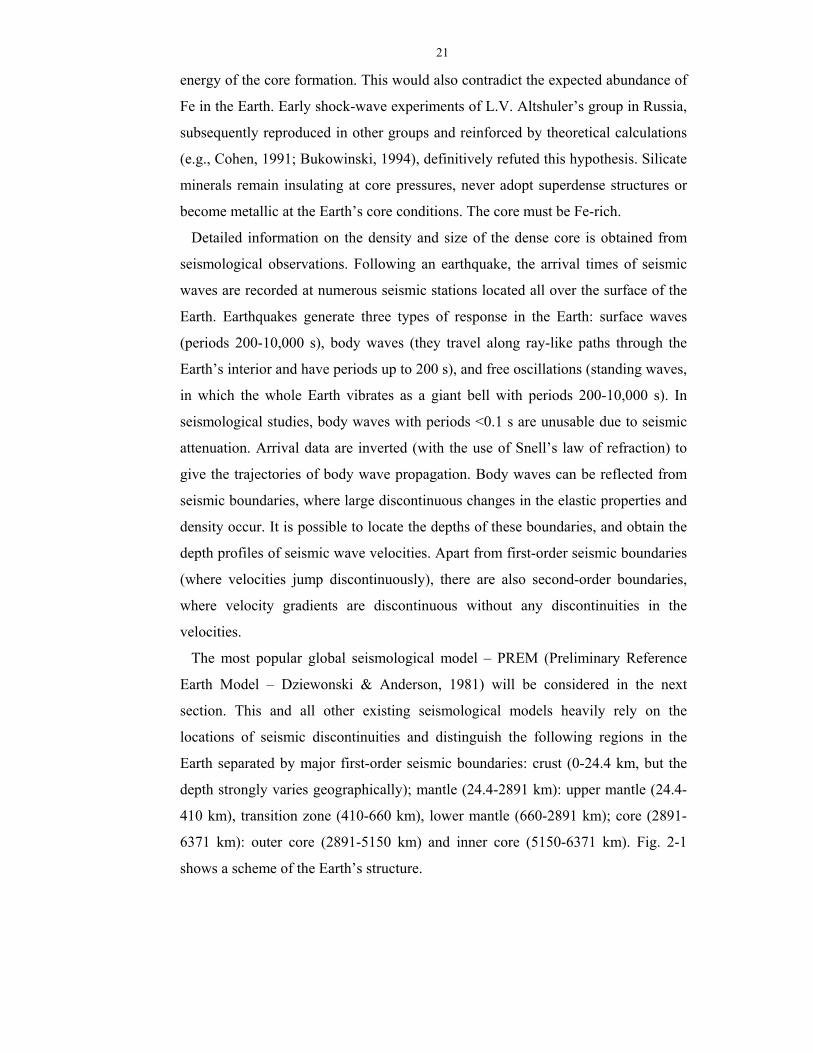
The most popular global seismological model – PREM (Preliminary Reference
Earth Model – Dziewonski & Anderson, 1981) will be considered in the next
section. This and all other existing seismological models heavily rely on the
locations of seismic discontinuities and distinguish the following regions in the
Earth separated by major first-order seismic boundaries: crust (0-24.4 km, but the
depth strongly varies geographically); mantle (24.4-2891 km): upper mantle (24.4-
410 km), transition zone (410-660 km), lower mantle (660-2891 km); core (2891-
6371 km): outer core (2891-5150 km) and inner core (5150-6371 km). Fig. 2-1
shows a scheme of the Earth’s structure.

22
Fig. 2-1. Scheme of the Earth’s internal structure. Earth’s mantle and outer core
convection are shown here. Mantle convection is responsible for plate tectonics,
core convection – for the the generation of the Earth’s magnetic field (whose force
lines are also shown). From
http://geoweb.princeton.edu/faculty/Duffy/MineralPhy/index.htm (taken from the
book Lamb S., Sington D. Earth story: the shaping of our world. London : BBC
Books, 1999, 240 pp.)
It is noteworthy that there are other models of the Earth’s internal structure,
differing in the stratification of the mantle – see, e.g., Pushcharovsky and
Pushcharovsky (1999), who distinguish 6 layers in the mantle and consider both
major and minor discontinuities as region boundaries (layers 30-400 km, 400-670
23
km, 670-850 km, 850-1700 km, 1700-2200 km, 2200-2900 km). However, this and
other similar schemes can be accepted only when the global nature and first-order
character of the minor discontinuities are proved.
Seismic observations detect these minor discontinuities only in some regions, but
it must be kept in mind that even global discontinuities may become seismically
unobservable if they are small enough and/or spread over a large depth interval. As
a rule of thumb (Helffrich, 2000), they become undetectable if their thickness
exceeds ¼ of the wavelength of the incident seismic wave. The finite thicknesses of
the discontinuity zones are primarily due to lateral variations of temperature
(Helffrich, 2000) and the dependence of the phase transition pressures (and depths)
on temperature via the Clapeyron relation: dp/dT=∆S/∆V. Finite thickness of phase
transition boundaries in the mantle is also due to the multicomponent composition
of the mantle. In effect, the discontinuities related to phase transitions with large
Clapeyron slopes and/or having large two-phase coexistence regions on the phase
diagram may become locally or globally seismically invisible. This is the case for
the global 520-km discontinuity related to the wadsleyite-ringwoodite transition:
this discontinuity is small and only locally observable (Shearer, 1990); it is not
included in current seismological models.
2.5. PREM and other spherical models.
PREM is the most frequently used seismological model of the Earth. Other
models (e.g., ak135 – Kennett et al., 1995) generally agree with PREM within 1-2%
on seismic velocities (Fig. 2-2). The parameters given by all these models as a
function of depth are: pressure (p), compressional and shear seismic velocities (VP
and VS), density (ρ), acceleration due to gravity (g), adiabatic bulk and shear moduli
(KS and G), seismic parameter (Φ=KS/ρ), Poisson ratio (ν), attenuation Q-factors
for the compressional and shear velocities (QP and QS), and Bullen parameter (η).
PREM velocity profiles are shown in Fig. 2-3, while Fig. 2-4 and Fig. 2-5 show
profiles of the density and pressure, respectively.

24
Fig. 2-2. Comparison of the PREM and ak135 profiles of seismic wave
velocities in the Earth’s mantle and crust. Generally, the agreement is good.
Serious differences are in the ultralow velocity zone (~220 km depth); gradients of
seismic wave velocities in the upper 670 km are significantly different. In the lower
mantle, the velocity profiles of the two models practically coincide.
Within PREM there are a number of observables: 1) mass of the Earth, 2)
geometrical parameters of the Earth (geoid data), 3) moment of inertia of the Earth,
and 4) seismic data – arrival times of seismic waves, from which it is possible to
obtain the trajectories of propagation of the seismic waves including locations
where reflection of seismic waves occurs, in particular 5) locations of seismic
boundaries. Studying reflection and refraction of seismic waves in the Earth’s
interior, it is possible to locate seismic discontinuities quite precisely (Helffrich,
2000).
In constructing PREM (Dziewonski and Anderson, 1981; see also Poirier, 2000),
measured geometry, mass and moment of inertia of the Earth were used, and it was
assumed that in each continuous region below 670 km the Adams-Williamson
equation:
dρ/dr=-gρΦ 1−S , (2.5.1)
describing adiabatic self-compression of a chemically homogeneous material, is
valid. For the upper mantle, the Birch’s law density-velocity systematics (VP=

25
a(−
M ) + bρ, where a and b are constants – see section 3.13) was assumed to apply.
At the start, values for the density of the Earth’s surface rocks (3.32 g/cm3), at the
core-mantle boundary (5.5 g/cm3) and the density jump at the inner-outer core
boundary (0.5 g/cm3) were supplied, and subsequently refined. The provisional
density distribution thus obtained was then refined in a general fitting procedure
(fitted parameters: profiles of VP, VS, ρ, QP, and QS) with added observables (free
oscillation periods and travel times for the 1s-period P- and S-waves). The
uppermost 200 km were treated as an elastically anisotropic region.
Fig. 2-3. PREM seismic velocity profile. Major regions of the Earth are
specified. The core-mantle boundary region D’’ (grey shading) is the major seismic
boundary in the Earth and has many anomalous and poorly understood properties.
Pressure distribution can be calculated using the following equation:
dp/dr=-4πGρr-2 ∫r
0
ρ r2dr = -gρ, (2.5.2)
where G is the gravitational constant, and r is the radius.

26
Fig. 2-4. PREM density profile.
Fig. 2-5. PREM pressure profile. Pressure is continuous, but there is a large kink
in its slope at the core-mantle boundary due to the large density jump occurring
there.
2.6. Interpretation of PREM. Composition, mineralogy, and temperature.
It is straightforward (eq. 2.5.2) to calculate the pressure distribution from the
density distribution provided by seismological models. Derivation of a temperature
profile is much more complicated, and there is still no commonly accepted thermal
profile of the Earth. Determination of the composition of each region of the Earth
from seismological models is another non-trivial, yet fundamentally important,
problem.

27
As we saw, the core must be mainly made of Fe, with minor siderophile
(particularly Ni) content. Its density, however, is too low compared to pure Fe at the
core conditions (by ~6-10% in the outer core). This is explained by the presence of
lighter alloying elements. From Birch’s law (see section 3.13), the average atomic
mass −
M =49.3 (Poirier, 2000), supporting the presence of lighter elements (the
atomic mass of Fe is 55.8). On the basis of the latest theoretical work (Vočadlo et
al., 2000) and experiments, it is believed that the phase of Fe stable at the inner core
conditions, is hcp-Fe. From seismic observations it follows that the inner core is
highly seismically anisotropic, with the fastest direction of seismic waves along the
axis of the Earth’s rotation. This anisotropy implies a high degree of crystal
alignment, whose cause is unknown. Using ab initio molecular dynamics
simulations, Alfé et al. (1999) calculated the melting curve of pure Fe and
concluded that for a pure-Fe core the temperature at the inner-outer core boundary
is 6700 ± 600 K. Using the density jump at this boundary as a constraint, Alfé et al.
(2000 and private communication) were able to put forward a compositional model
for the Earth’s core (inner core: 8.5% Si+S and 0.2% O; outer core: 10% Si+S and
8% O); this composition has −
M =49.38. The temperature at which these
compositions are at equilibrium, is 5500 K. This is the best currently available
estimate of the core temperatures.
Convection of the outer core generates the Earth’s magnetic field. The giant
dynamo-mechanism is, most probably, powered by the energy released on cooling
of the core: 2.6*1012 from cooling itself, 0.34*1012 W from crystallisation of the
inner core, and 0.66*1012 W of gravitational energy due to the convective rise of
Fe-depleted liquid during crystallisation of the Fe-rich inner core (Verhoogen,
1980). By constructing an adiabatic temperature profile for the outer core, Alfé et
al. (private communication) obtained T~4300 K at the core-mantle boundary.
The Earth’s mantle consists mainly of Mg-silicates. Birch’s law gives −
M = 21.3
for the mantle. Compared to −
M = 20.12 for MgSiO3, 20.15 for MgO, and 20.13 for
Mg2SiO4, this implies an ~10% substitution of Mg by Fe. Fe is mainly in the form
of Fe2+, which is in a high-spin state at low pressures, but may transform into low-
spin Fe2+ at high pressures. This ‘magnetic collapse’ has attracted much attention in
both theoretical (Sherman, 1991; Isaak et al., 1993; Cohen et al., 1997; Cohen,
1999; Fang et al., 1999; Gramsch et al., 2001) and experimental (Pasternak et al.,

28
1997; Badro et al., 1999) literature. Despite many interesting implications of the
possible presence of low-spin Fe2+ in the mantle and a large number of studies, it
remains highly unclear whether the low-spin Fe2+ exists in the mantle. Phase
transitions of Mg-silicates determine the seismic stratification within the mantle
(Fig. 2-6; Helffrich, 2000; Chudinovskikh & Boehler, 2001). Whether there is a
compositional stratification, related to the phase transition boundaries, is an open
question. From phase diagrams of the Mg2SiO4-Fe2SiO4 system, Ito & Katsura
(1989) determined T=1673 K at 350 km and 1873 ± 100 K at 660 km depths.
If the mantle were chemically homogeneous and had a pyrolitic composition, the
lower mantle would consist of (Mg,Fe)SiO3 perovskite (~75 vol. %),
magnesiowustite (Mg,Fe)O (~20 vol. %), and CaSiO3 perovskite (~5 vol. %).
Atomistic simulations of Watson et al. (2000) have demonstrated that the solubility
of Ca in MgSiO3 perovskite is negligible; therefore, CaSiO3 perovskite must be
present as a distinct phase. There has been some experimental evidence (Meade et
al., 1995; Saxena et al., 1996, 1998) that at high mantle temperatures and
Fig. 2-6. Schematic phase relations in pyrolite (after Ringwood, 1991). OPX and
CPX are ortho- and clinopyroxene, ILM is MgSiO3 ilmenite (akimotoite), MW is
magnesiowüstite (Mg,Fe)O, ‘Mg-perovskite’ and ‘Ca-perovskite’ stand for MgSiO3
and CaSiO3 perovskites.

29
pressures >75 GPa, MgSiO3 perovskites breaks down into the mixture of oxides,
periclase (MgO) and post-stishovite phase of SiO2. However, there seems to be
more evidence (Shim et al., 2001; Serghiou et al., 1998; see also a technical
discussion in Dubrovinsky et al., 1999 and Serghiou et al., 1999) that MgSiO3
perovskite remains stable at mantle conditions. Knowledge of the thermoelastic
properties of (Mg,Fe)SiO3 perovskite is crucial for constructing thermal and
compositional models of the mantle. Stixrude et al. (1992), on the basis of first
measurements of thermoelastic parameters of (Mg,Fe)SiO3 perovskite (Knittle &
Jeanloz, 1986; Mao et al., 1991) with very high thermal expansion coefficient,
arrived at the conclusion that the lower mantle must be ~100% (Mg,Fe)SiO3
perovskite. This would imply a compositional difference between the lower mantle
and pyrolitic upper mantle, absence of chemical mixing between different parts of
the mantle and layered, rather than whole-mantle, convection. The total mantle
composition would be chondritic (e.g., in Mg/Si ratio), rather than pyrolitic. Later
measurements of thermal expansion of this mineral (Wang et al., 1994; Funamori et
al., 1996; Fiquet et al., 2000) yielded much lower values, strongly supported by ab
initio simulations of Oganov et al. (2001a). To have a pure-perovskite lower mantle
with these values, one must have temperatures ~2500 K at the top of the lower
mantle, inconsistent with the value of 1873 K determined by Ito & Katsura (1989).
Whole-mantle or intermediate convection models are currently preferred, being also
consistent with seismic tomography images (see next two sections). The main
support of the layered convection model comes from geochemical studies, which
indicate two chemically distinct sources of mantle magmas with different degrees of
depletion in volatiles. This geochemical observation can be explained by either
intermediate style of convection (i.e., with partial mixing) or by layered convection
taking place at earlier stages of the Earth’s evolution and then replaced by whole-
mantle convection, possibly about 1 billion years ago (see Poirier, 2000).
The temperature gradient in a convecting system must be adiabatic or higher. The
adiabatic temperature gradient can be calculated from the thermodynamic equality:
(∂T/∂p)S=γT/KS=αVT/CP , (2.6.1)
where V is the molar volume, and takes the form:
(dT/dr)S = -MαgT/CP , (2.6.2)
where M is the molar mass. For the lower mantle the adiabatic temperature gradient
is equal to ~0.3-0.4 K/km (Verhoogen, 1980).
30
A fundamental geophysical relation (see Jackson, 1998) exists:
1-g-1∂Φ/∂r = (∂KS/∂p)S + (ταΦ/g){1+(∂KS/∂T)P/αKS}, (2.6.3)
which describes self-compression of a chemically homogeneous layer characterised
by a superadiabatic temperature gradient τ; α is the thermal expansion coefficient.
If the temperature distribution is adiabatic, the following relation must be obeyed:
η = (dKS/dp)S + g-1dΦ/dr = Φdρ/dp = 1 , (2.6.4)
where η is known as the Bullen parameter. If its values deviate from 1, it indicates
that either the temperature gradient is non-adiabatic, or the chemical composition
varies with depth. The Bullen parameter can be calculated from seismological
models.
The superadiabatic gradient τ is related to the deviations of η from unity:
τ = (g/α)[Φ -1-dρ/dp] = (g/αΦ)(1-η) (2.6.5)
The effects of changing chemical composition can also be included, yielding the
following equation:
dρ/dp = Φ-1 - ατ/g + (ξ/ρg)(∂ρ/∂X)p,T , (2.6.6)
where X is a compositional variable, and ξ its gradient. It should be noted that
possible compositional heterogeneity and non-adiabatiity in the mantle have
opposite effects on η (Jackson, 1998).
In PREM, η=0.99±0.01 throughout the lower mantle, supporting the view that the
lower mantle is adiabatic and chemically homogeneous. However, in ak135 model
η=0.94±0.02, which implies very large superadiabatic gradients, 0.3-0.7 K/km
(Jackson, 1998).
According to Verhoogen (1980), the core-mantle boundary layer D’’ is essentially
a thermal boundary layer with a temperature jump of ~1200 K. This mysterious
layer is highly variable in its thickness, is highly heterogeneous and elastically
anisotropic, and has very small or in some places even negative velocity gradients.
An intriguing possibility is the partial melting of this region. Solidus of the pyrolite
mantle was determined experimentally by Zerr et al. (1998); at core-mantle
boundary melting would start at 4300 K. As this is remarkably similar to the
temperatures of the core near this boundary, partial melting of the lower mantle in
the D’’ seems very likely. The presence of a melt would imply a high electrical
conductivity due to ionic diffusivity. The electrical conductivity of the lower mantle
is indeed very high (~1-10 S/m – Xu et al., 2000); apart from partial melting it
could be explained (O’Keeffe & Bovin, 1979; Matsui & Price, 1991) by a

31
hypothetical temperature-induced phase transition of MgSiO3 perovskite from the
orthorhombic to a disordered and superionically conducting cubic phase. Knittle
and Jeanloz (1991) considered the D’’ as a chemical reaction zone between the core
and mantle. They experimentally observed a reaction, which can be schematically
written as follows:
(Mg,Fe)SiO3 + Fe = MgSiO3 + SiO2 + FeO + FeSi (2.6.7)
Iron oxide and silicide at the high pressure of the core-mantle boundary are metallic
and should be soluble in the core. The reaction of Knittle and Jeanloz (1991) might
drive Fe (as well as Si and O) from the mantle into the core. This opens an
interesting possibility of the still growing core.
Another interesting question is the nature of minor seismic discontinuities in the
lower mantle. E.g., the locally observed 1200-km discontinuity (Vinnik et al., 1998;
Le Stunff et al. (1995) suggested that discontinuities at 785-950 km and 1200 km
might be global) has been attributed to a tetragonal-to-cubic transition in CaSiO3
perovskite (Stixrude et al., 1996; Chizmeshya et al., 1996) found in linear-response
all-electron LAPW calculations. More approximate pseudopotential calculations of
Karki (1997) and Warren et al. (1998), however, did not find this transition, and the
stable phase of CaSiO3 perovskite in their simulations was always cubic. Improved
experimental and theoretical techniques can or soon will be able to resolve such
these questions.
Closely related to the (still unknown) composition is the problem of the lower
mantle mineralogy. Mineralogical models significantly differ in mineral
proportions; essentially nothing certain is known about the mineralogy of Al. This
question may have far-reaching consequences, and it will be considered in detail in
Chapter 8.
Our understanding of the mantle mineralogy can be greatly increased by studies
of mantle inclusions – e.g., Harte et al. (1999) found several lower-mantle minerals
(among others, they found MgSiO3 inclusions with up to 10% Al2O3) in inclusions
in diamonds. Most inclusions studied so far have upper-mantle or transition-zone
origin, however.
The transition zone (410-660 km) is quite diverse mineralogically, and might
possess exotic properties. This region can host large amounts of water: both
wadsleyite and ringwoodite can contain up to 2-3 wt.% H2O (see Fiquet, 2001 and
references therein). It has also been suggested (Angel et al., 1996 and references
32
therein) that unusual for inorganic compounds five-coordinate Si can play an
important role in the transition zone, determining its transport properties.
The upper mantle consists predominantly of olivine, garnet, and pyroxenes. There
are four particularly important features of the upper mantle: 1) Ultralow velocity
zone at variable depths, roughly between 50-100 km and 220 km (Anderson, 1989),
2) A seismic discontinuity (Lehmann discontinuity) at the base of the ultralow
velocity zone, 220 km depth, 3) Strong elastic anisotropy above the 220 km depth,
and 4) Strong compositional heterogeneity in the upper 150 km (see Ringwood,
1991). The Lehmann discontinuity is, possibly, due to the Pbca-C2/c transition in
pyroxenes (see Mendelssohn & Price, 1997). The ultralow velocity zone is
interpreted as a region of partial melting and low viscosity (asthenosphere) beneath
the rigid lithosphere. Anisotropy in this region is a consequence of preferred
orientation of crystals caused by nearly horizontal convective flow of the mantle.
The uppermost parts of the upper mantle consist mainly of peridotites, while the
pyrolitic composition is believed to be characteristic of its deeper regions
(Ringwood, 1991).
A comprehensive review of mantle mineralogy can be found in Fiquet (2001).
Overall, mantle mineralogy is rather poor: only a handful of mineral species are
stable there, and all these minerals have quite dense structures. Very large (e.g., Na,
K, Rb, Cs, Ca, Sr, Ba, Cl, Br, I, S, Se, Te, U, Th) and very small (e.g., Li, Be, B)
atoms cannot enter these minerals, and concentrate in mantle magmas and fluids,
rising to the surface of the Earth and forming its crust. This is why the rich mineral
list of the crust is dominated by rare mantle-incompatible elements. The most
abundant minerals of the crust are feldspars (Na,K,Ca)(Al,Si)4O8. The chemical and
mineralogical composition as well as the thickness of the crust are very different
under oceans and continents. Basaltic oceanic crust is much younger; it is richer in
Mg and Fe and poorer in mantle-incompatible elements, denser, and only ~10 km
thick. Continental crust is sometimes very old (up to 3-4 billion years), very rich in
mantle-incompatible elements, and very rigid and thick (up to ~100 km). The
variable thickness and rigidity of the lithosphere (which includes the crust and the
rigid uppermost part of the upper mantle) and convection in the deeper mantle
result in plate tectonics. Depending on the rheological properties of the lithosphere,
there could be other dynamical regimes: e.g., rigid-lid regime (Tackley, 2000),
where the lithosphere is not perturbed by deeper convection (this regime is possible
for Mars).
33
2.7. The Dynamic Earth: plate tectonics and mantle convection.
Plate tectonics theory, that appeared in the 1960s, was a revolutionary step in
geology. It explained for the first time the strong localisation of earthquakes in
continental margins (plate boundaries), the existence of volcanic mid-ocean ridges
(rift zones), and continental drift. It is firmly established that it is the mantle
convection that drives plate tectonics mechanism.
Convection can occur only when the temperature gradient is equal to or higher
than the adiabatic gradient, eq. (2.6.2), or, in other words, when Bullen parameter
η ≤ 1 (see eq. 2.6.5). Another very important criterion is that the Rayleigh number
Ra, which measures the ratio of the buoyant force to the viscosity drag force, be
higher than the critical value, Rac. For the case of a liquid heated from below,
Ra = gαh3∆T/νκ , (2.7.1)
where h is the thickness of the layer, ∆T is the temperature difference between the
top and bottom, ν is the kinematic viscosity, and κ is the thermal diffusivity (which
is related to the thermal conductivity, K, via: κ = K/ρCP).
For the liquid heated from within,
Ra = gαρqh5/νκK , (2.7.2)
where q is the rate of internal heat production.
For both cases of heating from within and from below, the critical values Rac ≈
2*103. Inserting values characteristic of the mantle into (2.7.1) and (2.7.2), one gets
highly supercritical values, ~109 for heating within and ~106 for heating from below
(Poirier, 2000; Anderson, 1989).
Among other important physical parameters is the Péclet number, which measures
the ratio of the convected heat to the conducted heat:
Pe = vl/κ , (2.7.3)
where v is a characteristic velocity and l is a characteristic length. For the Earth
Pe≈103, indicating that convection dominates overall (Anderson, 1989). At the
boundary of two separately convecting layers, where there is no vertical convective
velocity, no heat is transported by convection. A thermal boundary layer must exist
between separately convecting layers; across this layer heat is transported by
conduction, and temperature gradient is highly superadiabatic.
The Prandtl number:
Pr = ν/κ (2.7.4)
34
is ~1024 for the mantle, indicating that the viscous response to a perturbation is
much faster than thermal response (Anderson, 1989).
The numbers defined above are important in understanding results of numerical
modelling of the mantle convection (for a discussion of early results, see
Verhoogen, 1980). Rayleigh numbers significantly exceeding the critical value
imply time-dependent (rather than steady) convection with many convective cells
(when Ra is comparable to Rac, only one convective cell would develop1). At such
high Rayleigh numbers convective flow may become intermittent; the period of
interittency for the Earth’s mantle is calculated to be ~100 million years. The
estimated horizontal wavelength of mantle convection is ~ 700 km (Verhoogen,
1980).
The Earth’s mantle is convecting with velocities of several mm/year. These
velocities are highly variable, and may be a few times lower in the lower mantle
due to its higher viscosity. Microscopically, this solid-state convection is not well
understood. It is possible that in different parts of the Earth it occurs by different
mechanisms – plastic flow, dislocational or diffusional creep.
Hot ascending plumes are born at thermal boundary layers (especially D’’). They
may be depleted in Fe as a result of the reaction (2.6.7) with the core. Depletion in
Fe would increase buoyancy of the plumes. Cold downgoing slabs consist of
basaltic oceanic crust and peridotitic upper-mantle rocks (Kesson et al., 1998).
Excess silica in the form of stishovite (SiO2) in the basaltic part of the slabs may be
removed as a result of partial melting (Ringwood, 1991). According to Kesson et al.
(1998), the slab material is intrinsically less dense than the pyrolitic lower mantle;
its negative buoyancy would be entirely due to the lower T. Even if this material is
able to sink to the core-mantle boundary, it will eventually rise again when
sufficiently heated up. This has led Kesson et al. (1998) to conclude that slabs
cannot reside at the D’’ for much longer than 500 million years. It is possible that
the basaltic component of the slab, being much less dense than the lower mantle at
~600-800 km depths, is delaminated and left in the transition zone (Kesson et al.,
1998). However, below 800-1000 km basalts should be significantly denser than the
pyrolitic mantle (Ringwood, 1991). Generally, slabs may have a difficulty in
penetrating the 670-km discontinuity due to the large increase of viscosity and 1 I.e. convection is described by a spherical harmonic with l=1. Higher-order harmonics appear on increasing the Ra/Rac ratio. These conclusions were reached for a convecting
35
density at this depth. It is possible that slab material accumulates at this depth and
from time to time falls through the discontinuity in ‘avalanches’ – this picture was
obtained in numerical simulations of convection (see Poirier, 2000 and references
therein).
Cold slabs would have a different mineralogy from the rest of the mantle, because
of the lower temperatures and different bulk chemical composition. An aluminous
phase (possibly, MgAl2O4 in the CaTi2O4 or CaFe2O4 structures – Kesson et al.,
1994, 1998) would be present in the lower-mantle slabs. H2O, liberated from
hydrous silicates at high pressures, might form ice VII in sufficiently cold slabs
(e.g., at 700 K and 15 GPa – Bina & Navrotsky, 2000).
Subduction zones with downgoing slabs are strongly correlated with seismically
active areas (e.g., Japan); hot plumes are situated below volcanic ‘hot spots’ (such
as Hawaii or Iceland). It is important to understand the 3D-thermal structure of the
mantle, in particular how cold are the cold slabs and how hot are the hot plumes
relative to the normal mantle. The temperature contrast between the slabs and the
hot regions must be related to the driving force of convection. Knowledge of the
lateral temperature variations can shed a new light on the mantle, its structure and
composition.
Studying topography of major seismic discontinuities, it is possible to get some
ideas on the lateral temperature varations (Helffrich, 2000), knowing the Clapeyron
slopes of the corresponding phase transitions. Most slabs turn out to be ~400-700 K
colder than the average mantle at 660 km; Tonga slab seems to be ~1200 K colder.
The temperature anomaly below the Iceland hot spot is estimated to be +180 K at
the 660 km depth (Helffrich, 2000). Studies of this kind are very important, but
restricted to the seismic discontinuity zones. It is possible to extract the same
information and many other important characteristics of the mantle, but without
such restrictions, from seismic tomography. The first physically sound attempt to
solve this problem was made by Oganov et al. (2001b; see Chapter 10), who found
the maximum temperature contrast between the cold and hot regions increasing
from ~800 K at 1000 km depth to ~1500 K at 2000 km and, possibly, over 2000 K
at the core-mantle boundary. The following section is dedicated to a brief
discussion of seismic tomography.
sphere. In a slab-shaped convecting layer, convection with Ra ≈ Rac follows hexagonal
36
2.8. Seismic tomography.
In seismic tomography, a large number of seismological measurements are
inverted to give 3D-distributions of seismic wave velocities. It is common to
represent results in terms of perturbations of seismic velocities relative to the
average velocity at each depth: e.g., ∆VS/VS. Various types of tomographic
inversions exist, including regional and global. Technical details of seismic
tomography inversion techniques can be found in (Anderson, 1989; Kennett et al.,
1998; Masters et al., 2000). The most recent tomography maps have similar
qualitative features and give the absolute velocity perturbations within ~25%
uncertainty. Perhaps, the most reliable global seismic tomography maps currently
available are those of Masters et al. (2000). Older higher-resolution maps of
Kennett et al. (1998) realistically give much narrower cold (high-velocity) zones,
but strongly underestimate amplitudes of the velocity variations (see Masters et al.,
2000). Tomographic images obtained in these works are shown in Fig. 2-7 and 2-8.
It is very difficult to obtain a reliable 3D-distribution of the density
(Romanowicz, 2001), therefore the interpretation must concentrate on the
velocities. In the first approximation, low velocities can be attributed to high
temperatures, and high velocities – to low-temperature slabs. This interpretation is
generally consistent with the expected convective flow patterns. There is a
remarkable correlation between surface tectonics and tomographic images down to
the core-mantle boundary. Most slabs penetrate the 660-km boundary and even
seem to reach the core-mantle boundary (Masters et al., 2000), although in some
tomographic images (Kennett et al., 1998) most slabs seem to disappear somewhere
between 1000 km and 2000 km depths.
From PREM, the relative perturbation of shear and compressional seismic wave
velocities due to pressure alone:
RT=(P
S
VV
lnln
∂∂ )T (2.8.1)
is 0.7 (Anderson, 1989). A similarly defined parameter,
Rp=(P
S
VV
lnln
∂∂ )p (2.8.2)
measuring the same ratio, but due to temperature effects alone, is much larger: it
increases from 1.7 to 2.6 between the depths of 1,000 km and 2,000 km as
determined by seismic tomography (Robertson & Woodhouse, 1996). honeycomb-like patterns (called Benard patterns).
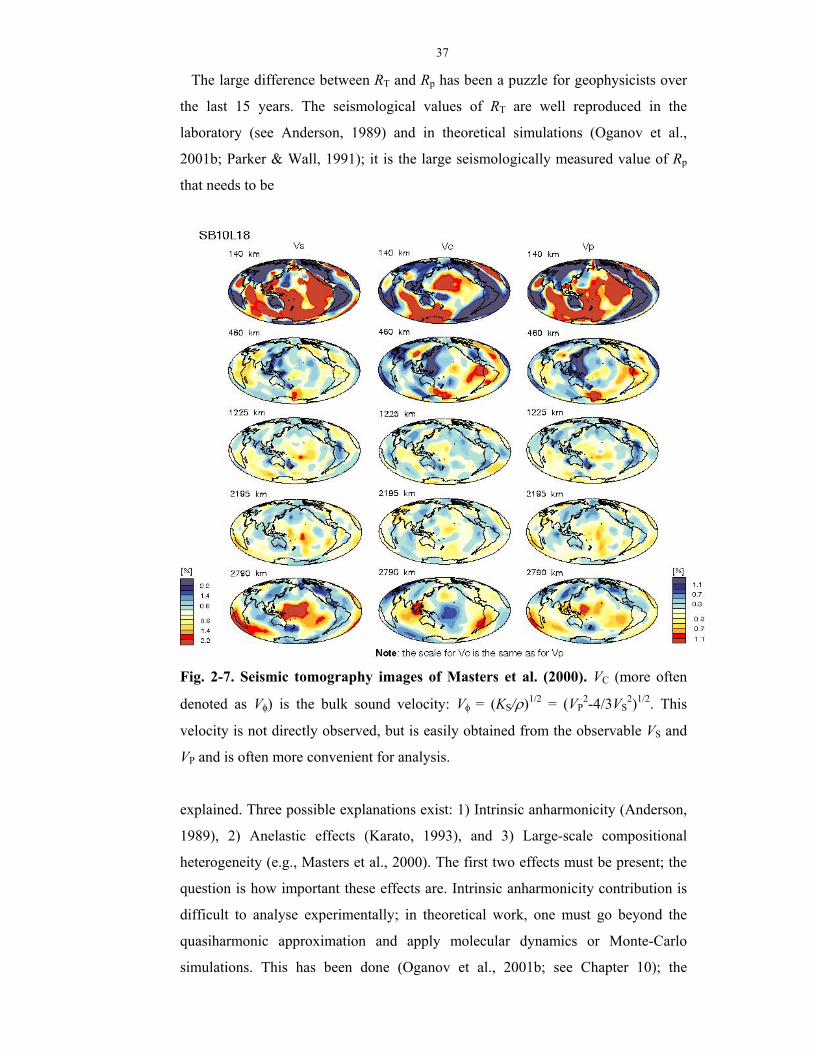
37
The large difference between RT and Rp has been a puzzle for geophysicists over
the last 15 years. The seismological values of RT are well reproduced in the
laboratory (see Anderson, 1989) and in theoretical simulations (Oganov et al.,
2001b; Parker & Wall, 1991); it is the large seismologically measured value of Rp
that needs to be
Fig. 2-7. Seismic tomography images of Masters et al. (2000). VC (more often
denoted as Vφ) is the bulk sound velocity: Vφ = (KS/ρ)1/2 = (VP2-4/3VS
2)1/2. This
velocity is not directly observed, but is easily obtained from the observable VS and
VP and is often more convenient for analysis.
explained. Three possible explanations exist: 1) Intrinsic anharmonicity (Anderson,
1989), 2) Anelastic effects (Karato, 1993), and 3) Large-scale compositional
heterogeneity (e.g., Masters et al., 2000). The first two effects must be present; the
question is how important these effects are. Intrinsic anharmonicity contribution is
difficult to analyse experimentally; in theoretical work, one must go beyond the
quasiharmonic approximation and apply molecular dynamics or Monte-Carlo
simulations. This has been done (Oganov et al., 2001b; see Chapter 10); the
38
resulting Rp is still lower than the seismological values, implying significant
anelastic and/or compositional contributions.
Anelastic attenuation springs from the dissipation of the energy of the seismic
wave passing through the rock. This effect is highly frequency-dependent, and has a
maximum at the frequencies similar to the frequency of some process (e.g., defect
migration) in the solid. Details of the complicated theory of attenuation can be
found in Anderson (1989); here I consider it briefly.

39
40
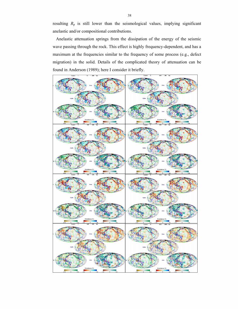
Fig. 2-8. Seismic tomography images of Kennett et al. (1998). In each box: top
left picture, Vφ perturbation; top right VS; centre VP perturbation; bottom left and
bottom right – distributions of (S
P
lnln
VV
∂∂ )p and (
Slnln
VV
∂∂ φ )p , respecively.
A wave travelling through an anelatic rock can be described by the following
wave equation:
A = A0exp[i(ωt-kx)]exp(-k*x) , (2.8.3)
where the wavenumber is complex, and k* is its imaginary part. For an anelastic
rock, the elastic constants are also complex (in Chapter 3 I shall consider in detail
the case of a perfectly elastic solid, where the elastic constants are real):
∧C = C + iC* , (2.8.4)
where C* is the imaginary part of a given elastic constant. The dimensionless
specific quality factor is
QM-1 = C*/C (2.8.5)
The Q-factor is related to the energy dissipation ∆ε per vibrational cycle:
Q = 4π<ε>/∆ε , (2.8.6)
were <ε> is the average energy of the wave. A model analytical expression for
Q(ω), taking into account its resonance nature, is:
Q-1(ω) = 2Qmax-1 2)ω(1
ωτ
τ+
, (2.8.7)
where τ is the relaxation time:
τ = τ0exp(H*/RT), (2.8.8)
where H* is the activation enthalpy. Eq. (2.8.8) explicitly introduces the
temperature dependence into the Q-factors. The frequency dependence of the
seismic wave velocities is approximately
V(ω) = V0(1+Qmax-1
2)ω(1ω
ττ
+) , (2.8.9)
where V0 is the zero-frequency velocity. The high-frequency (elastic) velocity is
simply
V∞ = V0(1+Qmax-1) (2.8.10)
Attenuation effects are usually negligble for the bulk modulus, but often are
strong for the shear modulus and shear seismic waves. Using PREM values of the
Q-factors in the lower mantle, (V∞-V0)/V0 is ~0.32% and ~0.13% for the shear and
41
compressional velocities, respectively (for the bulk velocities it would be only
0.002%). Dewaele and Guyot (1998) argued that PREM underestimates the
contribution of attenuation to the shear velocities in the lower mantle (i.e., PREM
values of Q are overestimated).
Karato (1993) proposed a method to estimate the contribution of anelasticity to
the seismologically measured Rp. Instead of (2.8.7) he used simpler expressions,
justifying it by the fact that in real solids there are usually several possible defect
relaxation mechanisms, rather than just one. The resulting Q-1(ω) function would
have many maxima and yield a smaller ω-dependence of the velocities than in the
model (2.8.9).
Karato (1993) considered two models. Assuming that Q is independent of ω, one
has
V(ω) = V∞[1+(Q-1/π)lnωτ] , (2.8.11)
from which Karato obtained
TV
∂∂ ln =
TV
∂∂ ∞ln
- [Q-1/π][H*/RT2] for Q>>1 (2.8.12)
In the second model, Karato allowed a small frequency dependence of Q:
Q(ω) ~ ωα with α~0.1-0.3 , (2.8.13)
in which case
V(ω) = V∞[1- ½cot(πα/2)Q-1(ω)] (2.8.14)
and
TV
∂∂ ln =
TV
∂∂ ∞ln - (πα/2)cot(πα/2)[Q-1(ω)/π][H*/RT2] for Q>>1 (2.8.15)
Karato estimated the anelastic contribution to Rp using H* for olivine. It became
clear from these estimates that the anelastic contribution is very important
throughout the mantle. Although no self-consistent analysis of the problem has been
reported for the lower mantle, it seems that the anharmonic and anelastic effects
would not be sufficient to account for the Rp values only in the D’’ layer. Some
other features of this layer (e.g., anticorrelation of the bulk and shear velocities –
see Fig 2-7) suggest that this region is significantly chemically heterogeneous on
large scales. This is hardly surprising if one views this layer as a chemical reaction
zone (Knittle & Jeanloz, 1991).
Forte and Mitrovica (2001) attempted to analyse seismic tomography data for the
core-mantle boundary. They took into account anharmonic, anelastic, and
42
compositional effects. Among other results, they reported on the temperature
contrast up to 1,200 K and maximum contrast in the Fe content of 2% (with hot
regions depleted in Fe). Unfortunately, their compositional derivative of the shear
wave velocity was almost certainly wrong by up to an order of magnitude, which
casts doubt on their results.
In the next chapter I shall consider in detail the elastic properties of crystals, their
equations of state, and thermodynamic properties. Theory presented in Chapter 3
plays a central role in the interpretation of seismological data.

43
Chapter 3. Thermodynamics, equations
of state, and elasticity of crystals.
In this chapter I shall discuss some of the most important properties of crystals –
their equations of state, elastic properties, and thermodynamic functions. As
thermodynamics is in the very heart of this whole area of solid state physics, I begin
the discussion with thermodynamic properties of crystals.
3.1. Thermodynamic properties of crystals.
Thermodynamic properties are, perhaps, the most important properties of a crystal
– they define its stability field; their derivatives with respect to pressure,
temperature, and volume describe the behaviour of the crystal at changing
conditions, its equation of state and response functions such as elastic constants and
thermal expansion.
In thermodynamic theory of condensed matter, a fundamental role is played by
the partition function:
Z = ∑ −
i
TkEe i B/ , (3.1.1)
where the summation is carried out over all discrete energy levels of the system.
Once Z is known, all thermodynamic properties can be obtained straightforwardly,
e.g. the Helmholtz free energy:
F = E0 – kBTlnZ , (3.1.2)
where E0 is the ground-state energy (at 0 K) including the energy of zero-point
motion.
However, it is extremely difficult to obtain all energy levels experimentally or
theoretically, and their number is overwhelmingly large for solids. This is where
simplified models (such as the harmonic approximation) come into play. The
harmonic approximation plays a key role in the theory of thermodynamic properties
of crystals. It gives a first approximation to the distribution of the energy levels Ei,
which is usually accurate for the most-populated lowest excited vibrational levels.
The key concept here is that of a non-interacting (ideal) gas of quasiparticles called
phonons, and the key quantity – the phonon density of states, g(ω), which defines the
number of phonons with energies in an infinitely narrow energy interval between hω
44
and hω+d(hω). The effects not accounted for by this simplified picture can often be
included as additive corrections to the harmonic results.
3.2. Harmonic approximation.
In the harmonic approximation it is assumed that all interatomic interactions are
analogous to perfectly elastic springs connecting atoms, the energy of any
displacement being proportional to the square of the displacement, x, and the force
induced by the displacement is proportional to the displacement itself:
∆E=1/2kx2 or E(R)= E(R0)+ 1/2kx2 , f=-kx , (3.2.1)
where R0 is the equilibrium distance between two atoms connected by a ‘spring’ with
a force constant k.
Quantum mechanics stipulates that energy levels be discrete, and for the harmonic
oscillator the solution of the Schrödinger equation yields the following energy levels:
En=h (1/2+n)ω, (3.2.2)
where n is the quantum number and ω the frequency of the vibration. For n=0
(ground state) there is a quantum energy hω/2 called the zero point vibrational
energy. For n=2,3,… we have doubly, triply,… excited vibrations – such vibrations
are called overtones, and due to high energies such excited states have low
populations pn, increasing with temperature according to the Boltzmann statistics:
pn~eTk
En
B
−
. Energy levels in a true vibrational system are well described by (3.2.2)
only for the lowest quantum numbers n, but these represent the most populated, and
thus the most important vibrational excitations.
In the harmonic model all atoms vibrate around their equilibrium positions.
Diffusion cannot occur as the energy required to remove an atom or for an atom to
become unbound to its original position, is infinite. Such high-temperature
phenomena as melting and diffusion in real materials cannot be accounted for by the
harmonic approximation. These phenomena are essentially anharmonic; the
harmonic potential (3.2.1) becomes inaccurate at large displacements (or, in other
words, high-order overtones are poorly described by the harmonic approximation).
These large displacements become accessible at high temperatures, where the
harmonic approximation breaks down. At not too high temperatures, however, the
harmonic approximation is valid.
In this approximation, the vibrational energy of the crystal can be determined via
the frequencies ω of the normal lattice vibrations (also known as vibrational modes
45
or phonons) and temperature T. Each normal mode contributes to the vibrational
energy according to a famous formula first derived by Einstein for the harmonic
oscillator:
Evib (ω, T) = 12hω +
1)ωexp(
ω
B
−Tkh
h , (3.2.3)
where h is the Planck constant, and kB the Boltzmann constant. The first term in
(3.2.3) is the zero-point energy originating from quantum motion of atoms; in the
harmonic approximation it is independent of temperature. Zero-point energy
dominates Evib at temperatures between zero and roughly half the Debye temperature.
The second, temperature-dependent term, gives the thermal energy of the mode
according to the Bose-Einstein distribution. The thermal energy (or heat content)
gives the energy absorbed by the crystal upon heating from 0 K to the temperature T.
At room temperature, the zero-point energy is usually significantly larger than the
heat content. Differentiating (3.2.3) with respect to the temperature, produces the
heat capacity of a harmonic oscillator :
CV,vib (ω, T) = (dT
TdE ),ω(vib )v = kB (TkB
ωh )22
B
B
)1)ω(exp(
)ω(exp
−Tk
Tkh
h
(3.2.4)
In the harmonic approximation the isochoric (CV) and isobaric (Cp) heat capacities
are equal: CV = Cp, and for the contribution of a normal mode to the vibrational
entropy of the crystal, we have:
Svib(ω, T) = dTT
TCT
∫0
p ),ω( = -kB ln[1-exp(TkB
ωh− )] +
T1
1)ωexp(
ω
B
−Tkh
h (3.2.5)
In a crystal with n atoms in the primitive unit cell, there are 3n different normal
modes. The Helmholtz free energy of a harmonic oscillator is then:
Fvib(ω, T) = 21hω + kB Tln[1-exp(
TkB
ωh− )] (3.2.6)
If all of them had the same frequency (the assumption of the Einstein model),
then, multiplying the right-hand sides of (3.2.3)-(3.2.6) by the total number of
vibrations (3n), all thermodynamic properties would be obtained immediately.
However, normal mode frequencies form a spectrum; most modes are in the infrared
range of frequencies. The highest frequencies are determined by the strongest bonds

46
in the structure. This spectrum of frequencies (energies) of phonons is called the
phonon spectrum, or phonon density of states g(ω).
As in the harmonic approximation the normal modes are independent of each
other and non-interacting, all thermodynamic properties can be obtained as a natural
generalisation of (3.2.3)-(3.2.6) by integration over all frequencies:
Evib(T) = ∫max
0
ω
vibE (ω, T)g(ω)dω =
= ∫max
0
ω
21hω g(ω)dω + ∫
max
0
ω
1)ωexp(
ω
B
−Tkh
h ]g(ω)dω (3.2.7)
CV(T) = ∫max
0
ω
vC (ω, T)g(ω)dω = kB ∫max
0
ω
(TkB
ωh )22
B
B
)1)ω(exp(
)ω(exp
−Tk
Tkh
h
g(ω)dω (3.2.8)
S(T)= ∫max
0
ω
S (ω, T) g(ω)dω =
= ∫max
0
ω
[-kB ln[1-exp(TkB
ωh− )] +
T1
1)ωexp(
ω
B
−Tkh
h ]g(ω)dω (3.2.9)
F(T) = E0 + ∫max
0
ω
F (ω, T)g(ω)dω =
E0 + ∫max
0
ω
21hω g(ω)dω + kB T ∫
max
0
ω
ln[1-exp(TkB
ωh− )]g(ω)dω , (3.2.10)
where E0 is the energy of the static lattice.
3.3. Models of the phonon spectrum: Debye, Agoshkov, Kieffer.
Once the density of states g(ω) is known, the application of equations (3.2.7)-
(3.2.10) is straightforward. IR- or Raman spectra probe only some of the vibrations
which have wavevectors close to zero (e.g., have the wavelengths of the scale of the
whole crystal; however, most vibrations have shorter wavelengths), and therefore do
not give the full information on the phonon spectrum. The g(ω) can be determined
experimentally by inelastic neutron scattering (e.g., Dove, 1993), or theoretically
using lattice dynamics or molecular dynamics simulations. All these methods are
complicated. Often one can obtain a reasonable approximation of g(ω) using the

47
easily obtained IR- and/or Raman spectra and/or elastic properties of the material.
Here I briefly describe such models.
Debye model. For the acoustic modes the phonon spectrum can be described, to a
first approximation, as a parabolic function truncated at the maximum frequency ωD
= h
Dθk . The Debye model assumes the same distribution for all phonon modes:
g(ω) = 9n(DθBk
h )2ω2 , (3.3.1)
where n is the number of atoms per unit cell of the volume V0, and θD is the
characteristic Debye temperature, the only parameter in this model.
With (3.3.1) for g(ω) the thermodynamic functions take the following forms :
Evib = 89 kBnθD + 3kBnTD(
TDθ ) , (3.3.2)
CV (T) = (dT
dE vib )v = 3kBn [4D(TDθ ) -
1/e
)/(3 D
D
−TT
θθ ], (3.3.3)
S(T) = dTTCT
∫0
p = kBn [4D(TDθ ) - 3 ln(1- TD /eθ ) ], (3.3.4)
where D(x) = 33x ∫ −
x
xdxx
0
3
1e , x =
TDθ .
The first term in (3.3.2) is the zero-point energy in the Debye model, the second
term is the heat content. The Debye temperature is determined by the elastic
properties of the solid – or, more precisely, its average sound velocity <v>:
θD = Bkh (
0
26V
nπ )1/3 <v> (3.3.5)
The mean sound velocity can be accurately calculated from the elastic constant
tensor (Robie & Edwards, 1966). Usually, however, an approximate formula is used:
<v> = ( 31
PV+ 3
2
sV)-1/3 , (3.3.6)
where VP and VS are the longitudinal and transverse sound velocities, respectively.
Later in this chapter, when discussing elastic constants, I shall discuss how to
calculate these velocities.
The Debye model is very effective in application to chemically and structurally
simple crystals, but in more complicated cases (particularly, in molecular crystals
and compounds with complex anions, e.g. silicates) it becomes too crude. Deep
theoretical analyses of this model and its critique can be found in (Seitz, 1949;
48
Kieffer, 1979a). Some more details of this model will be discussed in Chapter 10. As
will be also discuss later, the thermal equation of state can be formulated within the
Debye model – the roots and consequences of such approaches will be considered for
MgSiO3 perovskite.
Kieffer model. The most complete critical review of the Debye model can be found in
the paper by S.W. Kieffer (Kieffer, 1979a), who in the same seminal cycle of papers
proposed a new model (Kieffer, 1979b, 1979c, 1980, 1982). This much more
accurate model is based on the following main points: 1) Three acoustic modes have
a sinusoidal dispersion law ω(k) (not linear, as assumed in the Debye model) and are
described by three different densities of states, 2) Optic modes are divided into two
groups: high-frequency (e.g., Si-O stretching modes in silicates) and low-frequency
modes (e.g., cation-oxygen stretching modes and deformational modes). Low-
frequency vibrations are represented by an ‘optic continuum’ – a constant density of
states between some lowest ωl and highest ωu frequencies. In estimating these
limiting frequencies one is guided by the corresponding IR- and Raman frequencies
and the ratio of the masses of the cation and the complex anion – this approximately
takes into account the dispersion. The high-frequency modes are described by one or
more monochromatic (‘Einstein’) peaks of the density of states or another optic
continuum. The predictive power of this model is limited: the results critically
depend on the limiting frequencies ωl and ωu of the low-frequency optic continuum.
These frequencies differ greatly from crystal to crystal and therefore cannot be
transferred. Either an experiment or accurate calculations of the phonon spectrum are
required. At the same time, the Einstein frequencies are usually quite transferable:
e.g., the Si-O stretching modes in orthosilicates have an average frequency of 28.5
THz.
Agoshkov model. One of the possible simplifications was introduced by V.M.
Agoshkov (Agoshkov, 1985; Agoshkov et al., 1994). This model was used in my
early work (Urusov et al., 1998). In brief, all the acoustic and low-frequency optic
modes are described by a single Debye-like parabolic density of states g(ω) (3.3.1),
but truncated (such truncation was also present in Kieffer’s model) at a lower
frequency; this maximum frequency ω *D is now:
ω *D =
h
DBθk 3
33
nM+ , (3.3.7)

49
where M is the number of the low-frequency optic modes, included in the parabolic
g(ω). The high-frequency modes, like in the Kieffer model, are described as Einstein
oscillators.
The zero-point energy of the Agoshkov model is easily obtained:
Ezp = 89 kBnθD (
nM
33 + )4/3
+ ∑−
+=
33
1iω
21n
Mih , (3.3.8)
where the first term gives the contribution of the ‘Debye distribution’, and the second
term is a sum over all the high-frequency optic modes. Expressions for other
thermodynamic functions were given in the original work (Agoshkov, 1985). Very
accurately describing heat capacity at room and higher temperatures, the model gives
serious errors at low temperatures; this affects the entropy. The same shortcoming is
possessed, but to a smaller extent, by the Kieffer model. The advantage of the
Agoshkov model is in its suitability for the a priori estimates of thermodynamic
properties. Anharmonic corrections can be easily incorporated into both models (for
the Debye model this is even easier – I shall discuss this in Chapter 10) by assigning
different values of the mode Grüneisen parameter to each group of vibrations.
It is possible to construct other approximate thermodynamic models – an example
is the Komada-Westrum model (Komada & Westrum, 1997), which, like the Debye
model, has only one parameter, but is comparable in its accuracy to more
complicated models.
3.4. Shortcomings of the harmonic approximation.
The harmonic approximation, neglecting third- and higher-order terms in the
interatomic potential, leads to a number of fundamental errors. First, within this
approximation, all vibrational modes are independent – there is no exchange of
energy and momentum between them. This leads to a simple interpretation of
experimentally observed vibrational spectra and greatly simplifies the calculation of
thermodynamic properties (3.2.7)-(3.2.10), but at high temperatures errors become
serious.
Non-interacting phonons can freely travel within the crystal, leading to the infinite
thermal conductivity of the harmonic crystal. In real crystals, thermal conductivity is
finite due to phonon-phonon collisions (especially Umklapp processes – see Elliott,
1998), scattering on defects, and finite size of samples.
50
As it was mentioned, diffusion and melting cannot be explained within the
harmonic approximation. The same can be said about displacive phase transitions –
although the harmonic approximation can indicate such a transition by showing a
soft mode, no properties can be calculated for the dynamically disordered phase.
In the harmonic approximation there is no thermal expansion, which obviously
contradicts experiment. This is particularly important for geological applications.
Related to this is the equality CV=Cp, whereas experiment indicates CV < Cp.
From general thermodynamics, we have:
Cp = CV(1+α2KTV/CV) , (3.4.1)
where α is thermal expansion coefficient, KT isothermal bulk modulus, and V the
molar volume. When α = 0, CV=Cp.
Also, experiment indicates (Gillet et al., 1999) that at high temperatures the
isochoric heat capacity increases beyond 3nR (the Dulong-Petit limit): CV>3nR,
while in the harmonic approximation 3nR is the maximum value. Similarly, the
vibrational energy can exceed the harmonic quota of 3kBT per atom. Consider a
single anharmonic oscillator, whose potential is given by a polynomial expansion in
terms of displacements x from the minimum energy position:
Epot = 1/2kx2 + 1/3ax3 + 1/4bx4 + 1/5cx5 + … (3.4.2)
Applying the virial theorem (Landau & Lifshitz, 2001a, 1980): ½< xx
E∂
∂ pot > =
<Ekin>, we find for the expectation value of the kinetic energy:
<Ekin> = 1/2k<x2>+1/2a<x3>+1/2b<x4>+1/2c<x5>+…, (3.4.3)
which is kBT/2 at high temperatures – just like in the case of the ideal gas. Obvously
from (3.4.2), the potential energy is:
<Epot> = 1/2k<x2>+1/3a<x3>+1/4b<x4>+1/5c<x5>+…, (3.4.4)
and the total vibrational energy is:
<E> = <Ekin> + <Epot> = 22BTk - (a/2-a/3)<x3>-(b/2-b/4)<x4>-(c/2-c/5)<x5>-… =
=kBT –1/6a<x3>-b/4<x4>-3c/10<x5>-… (3.4.5)
To the lowest order,
<E> = kBT –1/6a<x3>, (3.4.6)
which should be >kBT since usually a<0 and <x3> > 0. Obviously, the second term in
(3.4.6) would be absent in the harmonic approximation, and we would recover the
Dulong-Petit value of kBT for the energy per mode at high temperatures.
51
Perhaps, the most spectacular failure of the harmonic approximation is its wrong
conclusion that vibrational frequencies do not depend on temperature and pressure.
To account for such experimentally observed strong dependences, one has to use
more realistic interatomic potentials. The first approximation, combining the
simplicity of the harmonic approximation and correcting its most serious errors, is
the quasiharmonic approximation.
3.5. Quasiharmonic approximation (QHA).
In this approximation, it is assumed that the solid behaves like a harmonic solid at
each volume, but the phonon frequencies depend on volume. It is assumed that they
depend only on volume – i.e., heating at constant volume does not change the
frequencies.
In the QHA phonon modes are still independent and non-interacting.
Thermodynamic functions at constant volume, as before, are given by (3.2.7)-
(3.2.10). Isochoric heat capacity CV still cannot exceed 3nR. Melting, diffusion, and
dynamically disordered phases are beyond the scope of this approximation, which
breaks down at high temperatures. Thermal conductivity is still infinite.
However crude, this approximation heals the biggest errors of the harmonic
approximation. Introducing a volume dependence of the frequencies is enough to
create non-zero thermal expansion and account for CV < Cp (cf 3.4.1). Thermal
pressure contributes to all constant-pressure thermodynamic functions (enthalpy H,
Gibbs free energy G, isobaric heat capacity Cp, etc.). This is the first approximation
for the thermal equation of state of solids, which can be effectively used in
conjunction with realistic interatomic potentials (Parker & Price, 1989; Kantorovich,
1995; Gale, 1998) or quantum-mechanical approaches (Baroni et al., 1987, 2001;
Karki et al., 1999, 2000a,b). It leads to some fundamental results, which remain
almost intact in more accurate theories. I shall concentrate on these issues later in
this chapter.
3.6. Beyond the QHA: intrinsic anharmonicity.
At temperatures roughly below one half to two thirds of the melting temperature,
QHA is quite accurate. Only at higher temperatures do its errors become significant.
All the effects beyond the QHA are termed intrinsic anharmonic effects. To the
lowest order, intrinsic anharmonic contribution to the free energy Fa is proportional

52
to T2 (Zharkov & Kalinin, 1968; Gillet et al., 1999; Dorogokupets, 2000) at high
temperatures:
F(V,T) = Fqha(V,T) + 3nkB[21 a(V)T2+…] , (3.6.1)
from which
E(V,T) = Eqha(V,T) - 3nkB[21 a(V)T2+…],
S(V,T) = Sqha(V,T) - 3nkB[a(V)T+…],
CV(T)= CV,qha(T) - 3nkB[a(V)T+…]
(3.6.2)
The use of (3.6.1) and (3.6.2) is restricted to high temperatures only, because at
low temperatures these equations will dramatically overestimate heat capacity (linear
instead of T3 temperature dependence) and lead to large errors in the entropy. An
exponential term better describes the effects of intrinsic anharmonicity in the whole
temperature range (Dorogokupets, 2001):
F(V,T) = Fqha(V,T) - 3nkB[k(V)Texp(-Q/T)+…] , (3.6.3)
where k is a constant, and Q parameter equal to or exceeding the melting
temperature. From (3.6.3) obtain:
E(V,T) = Eqha(V,T)+ 3nkB[k(V)Qexp(-Q/T)+…] ,
S(V,T) = Sqha(V,T) + 3nkB[k(V)(1+Q/T)exp(-Q/T)+…] ,
CV(T)= CV,qha(T) + 3nkB[k(V)(Q/T)2exp(-Q/T)+…] (3.6.4)
The exponential term is explicitly related to the premelting processes, involving
atomic diffusion and formation of thermal defects. These processes are linked to
melting in the Lennard-Jones and Devonshire model (Poirier, 2000), and are
essentially anharmonic. The exponential expression for the intrinsic anharmonic
effects leads to an excellent description of thermodynamic properties and thermal
equation of state of NaCl (Dorogokupets, 2001) at temperatures between 10-20 K
and the melting temperature.
One important consequence of intrinsic anharmonicity is that vibrational
frequencies depend not only on the volume; identical volume changes, produced by
changing pressure and temperature, result in different changes in the frequencies.
This is clearly demonstrated by precise experiments (see, e.g., Gillet et al., 2000;
1999) and computer simulations (Winkler & Dove, 1992). The intrinsic
anharmonicity parameter of an i-th phonon mode at a wavevector k is given by:

53
aik = (T
i
∂∂ kωln
)V = α(γikT-γik
p), (3.6.5)
where α is the thermal expansion coefficient, and γikT and γik
p are constant-
temperature and constant-pressure mode Grüneisen parameters (see below),
respectively. Intrinsic anharmonic parameters aik (3.6.5) are equal to the coefficients
a previously used in the expressions (3.6.1) and (3.6.2) for the anharmonic
thermodynamic properties (a expresses the total anharmonicity, while aik are the
mode anharmonic parameters). Since these parameters are measurable, the
anharmonic corrections can be directly evaluated from experiment. Soft modes are
the most anharmonic ones (above the critical temperature they are essentially
anharmonic), hence no wonder that thermodynamic functions of crystals near phase
transitions have anomalously large anharmonic contributions.
The full anharmonic theory of thermodynamic properties of crystals is very
complicated (for more details see Wallace, 1998); some details of phonon-phonon
interactions and their influence on thermal conductivity can be found in (Elliott,
1998). Computationally, all intrinsic anharmonic effects can be fully accounted for
by the use of Monte Carlo or molecular dynamics simulations (Allen & Tildesley,
1987): these methods involve a full sampling of the potential hypersurface without
any assumptions regarding its shape or the magnitude of atomic vibrations; these
methods are also applicable to liquids and gases. Free energies of significantly
anharmonic systems can be calculated using thermodynamic integration technique
(e.g., Allen & Tildesley, 1987; Alfé et al., 1999, 2000). An approximate method for
calculating anharmonic free energies was suggested by Wallace (1998) and used by
P. Gillet and co-workers (e.g., 1999; 2000). As Wallace has shown using
perturbation theory, the entropy S in the first approximation is given by the harmonic
result (3.2.9) when the actual frequencies are used (i.e. not quasiharmonically
extrapolated; one must take explicitly into account the temperature dependence of
the frequencies – eq. (3.6.5)). Other thermodynamic properties follow from this: e.g.,
CV(V,T)=T(∂S/∂T)V; note that only for the entropy can the original harmonic
expression be justified. Since the actual frequencies in this approach are
anharmonically corrected, so are the entropy, all other thermodynamic properties,
and the EOS.
We shall come back to anharmonic effects several times in this thesis. Now we
turn to the discussion of the thermal equations of state of solids.

54
3.7. Equation of state (EOS) – general thermodynamic formulation.
An equation of state (i.e., the p-V-T relationship) is one of the most important
characteristics of the Earth’s materials. Indeed, accurate EOSs of minerals are
necessary for the interpretation of seismological observations.
Generally, thermodynamics gives:
p = - (VF
∂∂ )T and V = (
pG
∂∂ )T isothermal EOS
T = (SH
∂∂ )p and S = -(
TG
∂∂ )p isobaric EOS
p = - (VE
∂∂ )S and V = - (
pH
∂∂ )S adiabatic EOS
An explicit analytical EOS can only be written for an ideal gas (where interatomic
interactions are absent: in this case there are no problems in the analytical
representation of the interatomic potential, and entropy can be easily and exactly
calculated using the Sackur-Tetrode relation). The classical ideal gas EOS is: pVm =
RT, where Vm is the molar volume.
For solids and liquids interatomic interactions are essential, and all existing
analytical EOSs are by necessity approximate. Even worse, interactions between
atoms make phase transitions possible, and EOS becomes discontinuous (i.e., non-
analytical) at phase transitions. All the approximate EOS formulations are valid only
for one phase, and generally the accuracy of the EOS is best at conditions far from
phase transitions.
To advance further, consider the isothermal EOS: p = -(VF
∂∂ )T , taking the QHA as
the starting point. Using indices i and k to denote the number of the phonon branch
and the wavevector k, we have:
F(T) = E0 + 21 ∑
k,ihωik + kBT∑
k,iln [1-exp(
TkB
iω kh− )]
and
p = -(VE
∂∂ 0 )T -
21 ∑
k,ih (
V∂∂ kiω )T - kBT∑
k,i(
VTk
∂
−−∂ )])ωexp(1(ln[B
ikh
)T , (3.7.1)
where the first term is the static (athermal) pressure, the second one counts the
pressure of the zero-point vibrations; and the third term represents the pressure
component associated with heating the crystal (thermal pressure). Simple
55
mathematical manipulations give the zero-point pressure pzp = -21 ∑
k,ih (
V∂∂ kiω )T =
21 ∑
k,ih
Vkk ii ωγ = <γik>Ezp/V, where we defined the mode Grüneisen parameter γik =
-(Vlnωln
∂∂ )T (in the QHA the constant-temperature and constant-pressure Grüneisen
parameters are equal). For the third term in (3.7.1) we similarly have:
pth = -kBT∑k,i
(V
Tk∂
−−∂ )])ωexp(1(ln[B
ikh
)T = ∑k
k
i,
i
Vγ
1)ωexp(
ω
B
i
i
−Tkk
kh
h = ∑k
k k
i,
i ith,
VEγ
,
where Eth,ik denotes the mode contributions to the thermal energy.
The total pressure is then:
p(V,T) = pst(V) + 21
∑k,i
hV
kk ii ωγ + ∑k
k k
i,
i ith,
VEγ
(3.7.2)
Defining average Grüneisen parameters, re-write eq. (3.7.2):
p(V,T) = pst(V) + <γik(V)>Ez.p.(V)/V + Γ(V,T)Eth(V,T)/V , (3.7.3)
where <γik> denotes the arithmetic average of the mode Grüneisen parameters γik,
and Γ is the so called thermodynamic Grüneisen parameter defined as a weighted
average of the mode Grüneisen parameters:
Γ = ∑
∑
kk
kk
k
i,ith,
ith,i,
i
E
Eγ =
th
ith,i,
i
E
E kk
k∑γ=
∑
∑
kk
kk
k
i,iV,
iV,i,
i
C
Cγ =
V
iV,i,
i
C
C kk
k∑γ, (3.7.4)
where CV,ik is the contribution of the i-th mode (at the k-wavevector) to the total
isochoric heat capacity (3.2.4).
From (3.7.3) and (3.7.4) one can derive thermal expansion:
α = Γ VK
CT
V (3.7.5)
Gathering the first two terms of (3.7.3), both describing the pressure at 0 K, and
neglecting the temperature dependence of Γ, one obtains the famous Mie-Grüneisen
thermal EOS:
p(V,T) = p0 K(V) + pth(V,T) = p0 K(V) + Γ(V)Eth(V,T)/V (3.7.6)
Note from (3.7.4) that at high temperatures, where all phonons are practically
fully excited, partial heat capacities CV,ik of all the phonon modes are very close to
their high-temperature limit (kB), and (3.7.4) reduces to a constant high-temperature

56
limit, which is just an arithmetic mean over all mode Grüneisen parameters: Γ →
<γik>.
In the classical approximation, which is put in the basis of the standard molecular
dynamics and Monte Carlo simulations, thermodynamic Grüneisen parameter will
always be close to <γik> (Welch et al., 1978), but also including a temperature-
dependent correction due to intrinsic anharmonic effects. Generally, Γ is a function
of not only volume, but also temperature – e.g. (3.7.4), where the weight of each γik
is given by the temperature-dependent CV,ik. Often Γ is a non-monotonic function of
the temperature (Oganov et al., 2000; Price et al., 1987). However, temperature
variations of Γ are usually small, rendering the original Mie-Grüneisen
approximation that Γ(V) is temperature-independent, rather accurate. The best value
to be accepted as Γ is <γik>, which is correct in the high-temperature limit, and which
also appears in the expression (3.7.3) in the pressure of zero-point vibrations.
Setting Γ = <γik> = γ, we can re-write the Mie-Grüneisen EOS as follows:
p(V,T) = pstat(V) + <γik>(V)Evib(V,T)/V = pstat(V) + γ(V)Evib(V,T)/V , (3.7.7)
which is more convenient for computer simulations than (3.7.6) due to the explicit
separation of the static pressure from the vibrational terms. Mie-Grüneisen EOS in
form (3.7.6) or (3.7.7) is the basis of most studies of thermal EOSs of minerals.
Despite being derived within the QHA, the Mie-Grüneisen EOS can be formulated at
any level of theory. Generally speaking, (3.7.4) will become invalid due to a
correction for intrinsic anharmonicity. For a general case it is convenient to define
the Grüneisen parameter via phonon pressure:
γ = vib
stat )](),([E
VVpTVp − (3.7.8)
Thermodynamic Grüneisen parameter can be defined via thermal pressure or
thermal expansion (cf. (3.7.5)):
Γ = th
K0 )](),([E
VVpTVp − = αKTV/CV (3.7.9)
The volume dependence of γ (or Γ) is usually described by a power law:
γ(V)=γ0(V/V0)q , (3.7.10)
where parameter q= (Vln
ln∂∂ γ )T is usually assumed to be constant, partly because of
the experimental difficulties in estimating q (Shim & Duffy, 2000). In many studies,
including mine (Oganov et al., 2000), it was found that q varies strongly with
57
volume; Oganov et al. (2001a) proposed a more accurate form, which seems to be
sufficient in the whole range of mantle pressures:
γ(V) = γ0(V/V0) )/ln( 010 VVqq + (3.7.11)
In (3.7.8)-(3.7.11) the intrinsic anharmonic effects are included implicitly within the
formalism derived within the QHA. Other approaches are possible.
Dorogokupets (2000, 2001) has proposed a model for fitting (and, possibly,
extrapolating) thermodynamic functions and equations of state of minerals in a broad
range of temperatures and pressures; in this model he explicitly separated
quasiharmonic and intrinsically anharmonic terms. Added to the quasiharmonic
thermal pressure from (3.7.8) (calculated with the quasiharmonic Eth), is the
anharmonic thermal pressure pa=-(VF
∂∂ a )T , where Fa is given by (3.6.1) or (3.6.3);
this pressure can also be recast in the Mie-Grüneisen-like form pa=γa(V)Ea(V,T)/V.
Expressing the anharmonic corrections to thermodynamic properties by (3.6.1)
and (3.6.2), i.e. making use of the approximate high-temperature result for each
mode Fa(ω,V,T) = 21 ai(V)kBT2, the anharmonic thermal pressure per mode is:
pa = -21 miaikBT2/V , (3.7.12)
where mi=(Va
lnln i
∂∂ )T . This result implies that when intrinsic anharmonic parameters
ai are volume-independent, the anharmonic thermal pressure will be negligible.
So far I have considered in detail the general construction of a thermal EOS. It has
not taken any analytical form yet. Various analytical formulations of the EOS are the
topic of next section.
3.8. Analytical representations of the equation of state.
The material discussed in this section can be found in several literature sources. I
mention here Poirier (1999, 2000), Poirier & Tarantola (1998), O.L. Anderson
(1995), Holzapfel (1996), Sutton (1993), Cohen et al. (2000), Vinet et al. (1986,
1989), and Angel (2001). The latter document is the manual to the program EOSFIT,
which I used for fitting pV-data to various EOSs.
Elasticity theory is used to construct the simplest EOSs. The simplest EOS is just
the definition of the bulk modulus: KT=-V(∂p/∂V)T. This EOS is valid only in a very
58
narrow pressure range, because the bulk modulus K changes rapidly with pressure.
The pressure variation of K is determined by the interatomic forces acting within the
solid – these forces must be accounted for by accurate EOS formulations.
Assuming that K varies linearly with pressure and denoting K0’=(∂K/∂p)T,p=0, we
obtain the Murnaghan EOS:
p = K0/K0’[(V/V0)-K0’ -1] (3.8.1)
This simple EOS works well in the compression range |(V-V0)/V0|<0.1-0.2. At larger
compressions higher-order derivatives of K become important. Of course, these non-
linearities can be formally incorporated as well, resulting in a more complicated
EOS. Better convergence is obtained if, instead of K as a function of pressure, we
construct an approximate model for the energy as a function of x=V0/V or some other
measure of strain. Using this method, some of the most popular EOSs are obtained –
families of Birch-Murnaghan and logarithmic EOSs of different orders. Vinet EOS
will follow from a general scaled interatomic potential.
Birch-Murnaghan EOSs. These EOSs are based on the polynomial expansion of the
energy:
E=E0+af 2+bf 3+cf 4+… (3.8.2)
in powers of the Eulerian strain fE:
fE = ½[1-(V0/V)2/3] (3.8.3)
It is advantageous to use the Eulerian finite strain rather than the Lagrangian strain:
fL = ½[(V/V0)2/3-1] , (3.8.4)
because Eulerian strain leads to a better description of the correct E(V) dependence
with fewer terms in the expansion (3.8.2). At infinite pressure, Eulerian strain is
infinite, whereas Lagrangian strain remains finite. However, for infinitesimal strains
both definitions become equivalent, and
dfE = dfL = da/a0 = -1/3(dV)/V0 (3.8.5)
It can be shown that generally
9V0K0 = (1/f)(∂E/∂f)T (3.8.6)
Truncating (3.8.2) on the second-order term:
E=E0+af 2, (3.8.7)
and, noting that
a=(9/2)K0V0, (3.8.8)
it is easy to obtain (see Poirier, 2000) the second-order Birch-Murnaghan EOS:
p = 3K0f(1+2f)5/2 (3.8.9)
59
Or, in a different form:
p = (3/2)K0[(V0/V)7/3-(V0/V)5/3] (3.8.10)
E = E0 + (9/8)K0V0[(V0/V)2/3-1]2 (3.8.11)
Third-order BM EOS is
p(V)=3/2K0[(V0/V)7/3-(V0/V)5/3]{1+ξ[(V0/V)2/3-1]}, (3.8.12)
E(V) = E(V0) +
+3/2K0V0[3/2(ξ -1)(V0/V)2/3+3/4(1-2ξ )(V0/V)4/3+1/2ξ (V0/V)6/3-(2ξ-3)/4],
(3.8.13)
where ξ=3/4(K0’-4).
Note that when K0’=4, the third-order Birch-Murnaghan EOS (BM3)
automatically reduces to the second-order one (BM2). In other words, BM2 EOS
implicitly assumes K0’=4. It is remarkable that this estimate of the lowest order of
the finite strain theory is often very close to experimental values of K0’ of many
crystals (especially with close-packed structures). This is why BM2 EOS, although
very simple, works well in many cases. The main problem of all BM EOSs is rather
poor convergence with respect to the number of terms beyond the second order for
large strains: it turns out that the fourth-order energy term in (3.8.2) is often larger
than the third-order one. The third-order BM EOS is very accurate when K0’ is close
to 4; when it is significantly different, this EOS gives poor results at high
compressions. For K0’<4 at large compressions (e.g., for V/V0~0.5 and K0’=2) BM3
can give even negative pressures (Poirier & Tarantola, 1998)! Being based on a
polynomial expansion of the interatomic potential (of the type ∑=
−
,...3,2,1
2n
n
nRa ), this EOS
must be used with caution when extrapolations are needed – outside the range of
fitting the truncated polynomial expansion (3.8.2) may become invalid (Cohen et al.,
2000).
It is possible to derive systematically higher-order BM EOS, but this appears to be
of little use since the number of parameters involved will be too large; only fourth-
order BM EOS:
p = 3K0fE(1+2fE)5/2{1+3/2(K0’-4)fE+3/2(K0K0’’+(K0’-4)(K0’-3)+35/9)fE2} (3.8.14 )
is sometimes used when ultra-high pressures are studied. This EOS is equivalent to
the BM3 EOS when K0’’=-1/K0{(3-K0’)(4-K0’)+35/9} – the value implied by the
BM3 EOS. BM4 EOS seems to be very accurate in a wide range of compressions –
insofar as can be judged from the limited number of its applications available.
60
Logarithmic EOSs. Drawbacks of the Birch-Murnaghan EOSs leave much room for
other possible EOSs. Poirier and Tarantola (1998) have derived the logarithmic EOS,
based on the polynomial expansion (3.8.2) in terms of natural, or logarithmic (also
called Hencky) strain:
fH = ln(l/l0) = 1/3ln(V/V0), (3.8.15)
where l is the length of the sample (l0 in the unstrained sample). The second-order
logarithmic EOS is:
p = K0(V0/V)ln(V0/V), (3.8.16)
implicitly assuming K0’=2. The third-order logarithmic EOS is:
p = K0(V0/V)[ln(V0/V)+1/2(K0’-2)(ln(V0/V))2], (3.8.17)
which implicitly takes K ''0 = -(1/K0)[1+(K '
0 -2)+(K '0 -2)2]. In the fourth order, the
logarithmic EOS is:
p=K0 VV 0 ln(
VV 0 )[1+
21 (K '
0 -2)ln(VV 0 )+
61 {1+K0K ''
0 +(K '0 -2)+(K '
0 -2)2}ln2(VV 0 )]
(3.8.18)
For the instructive case of hcp-Fe, Vočadlo et al (2000) have shown that the third-
order logarithmic EOS fits ab initio pV-data worse than third-order BM EOS (BM3)
or third-order Vinet EOS. Fourth-order logarithmic EOS is superior to BM3, but
involves more parameters. In the case of MgO examined in Table 1, the third-order
logarithmic EOS also shows a very poor performance compared to BM3 or Vinet
EOS. It can be expected that this EOS can work well in the rare cases where K0’~2.
Logarithmic EOS corresponds to an unphysical interactomic potential of the type
∑= ,...3,2,1
)(lnn
n Ra n (Cohen et al., 2000). Even though it can be expanded as –
a/R+bR )7'(3 0 −− K (Poirier & Tarantola, 1998), one can note that the repulsion exponent
is too small (5 for K0’=4) compared to the usual values ~9-12. This is why, although
based on a potentially powerful idea of the Hencky finite strain, the logarithmic EOS
is not successful. Like the BM3 EOS, the logarithmic EOS has an unphysical
behaviour on expansion (V/V0>1): the potential corresponding to BM3 behaves non-
monotonically, and the one corresponding to the logarithmic EOS diverges. Vinet
EOS is the best choice of an EOS for solids – it combines simplicity, high accuracy,
and universal applicability to solids with any character of chemical bonding, and up
to extremely high compressions (at least compression by 2-3 times).
Vinet EOS (Vinet et al., 1986, 1989). This EOS, also known as the Universal EOS, is
sometimes considered as one of the most impressive recent achievements of solid
61
state physics (Sutton, 1993). In fact, just like BM and logarithmic EOSs, Vinet EOS
is a whole family of EOSs of different orders. The most remarkable feature is very
fast convergence with respect to the order of EOS – one seldom needs to use higher
than third order Vinet EOS.
The third-order Vinet EOS is:
p = 3K0 3/20
3/10
)/()/(1
VVVV− exp[
23
(K '0 -1)(1-(V/V0)1/3] , (3.8.19)
E(V) = E(V0) + 2'0
00
)1(4
−KVK -
-2V0K0(K '0 -1)-2(5+3 K '
0 {(VV 0 )1/3-1}-3(
VV 0 )1/3)exp(-3/2(K '
0 -1){(VV 0 )1/3–1})
(3.8.20)
The value of K ''0 following is (Vinet et al., 1989): K ''
0 =-1/K0[(K '0 /2)2+(K '
0 /2)-
19/36]. The bulk modulus can be expressed as (Vinet et al., 1989):
K=(K0/( VV 0 )2/3)[2-(
VV 0 )1/3+{(
VV 0 )1/3-3/2(
VV 0 )2/3(K '
0 -1)}]exp(23 (K '
0 -1){1-(VV 0 )1/3})
(3.8.21)
This EOS is based on a universal scaled binding curve:
E =E0(1+a)exp(-a), (3.8.22)
where E0 is the bond energy at equilibrium, a=(R-R0)/l, l= )/(2
2
0
REE
∂∂ being a
scaling length roughly measuring the width of the potential well, and R the Wigner-
Seitz radius (the average radius of a sphere in the solid containing 1 atom). The
potential (3.8.19) was first used in 1930s by Rydberg for fitting potential curves of
molecules and obtaining their anharmonic coefficients; it turned out (see Sutton,
1993) that it describes very accurately systems with different types of chemical
bonding in solids, molecules, adsorbates, etc. The Vinet EOS proved to be very
accurate for fitting EOS of solid hydrogen (Loubeyre et al., 1996; Cohen et al.,
2000) throughout the whole experimentally studied pressure range 0-120 GPa,
roughly to the 8-fold compression. The universal binding curve (3.8.22), however,
does not describe long-range forces in ionic and van der Waals crystals. This means
that for such material Vinet EOS will not give accurate description of expansion
(V0/V<1). For compression, however, it should be sufficiently accurate, since
compression behaviour is dominated by interatomic repulsion, well accounted for by
(3.8.22).

62
In very rare cases a higher-order Vinet EOS may be needed; such higher-order
versions of the Vinet EOS already exist (Vinet et al., 1989); fourth-order Vinet EOS
has been successfully applied to solid H2 at extreme compressions (Cohen et al.,
2000) and has lead to significant improvements of the description of experimental p-
V data. At extreme compressions (V/V0<0.1), where solids approach the free electron
regime, other EOSs are required (Cohen et al., 2000). Such EOSs, manifesting the
Thomas-Fermi behaviour at extreme compressions, are developed and discussed in
detail by Holzapfel (1996) and Hama and Suito (1996); some discussion can also be
found in (Cohen et al., 2000).
Table 3-1 gives a summary of the EOSs discussed, while Table 3.2 gives a
comparison of several EOSs fitted to theoretical data on MgO. Fits were performed
in different pressure ranges. For a reliable (i.e., applicable for extrapolations) EOS,
fitted parameters (V0, K0, and K0’) should be independent of the pressure range of
fitting and consistent with zero-pressure values of these parameters. Zero-pressure
unit cell volume was fixed in our fitting; K0 and K0’ were determined from the
independently calculated elastic constants at zero and other pressures. The best
results can be obtained with the BM3 and Vinet EOS. For MgO BM3 slightly
outperforms Vinet EOS. However, there are more examples of the dramatically
opposite behaviour, and the overall performance of the Vinet EOS is better.
Logarithmic EOS is unreliable. In a finite pressure range the values of the EOS
parameters (especially K0’) can strongly depend on the EOS used. Note that as the
pressure range of fitting tends to zero, all EOSs recover the correct zero-pressure
parameters – the fastest convergence is for BM3 and Vinet EOSs. At small
compressions all EOSs become equivalent.
Table 3-1. Summary of analytical equations of state.
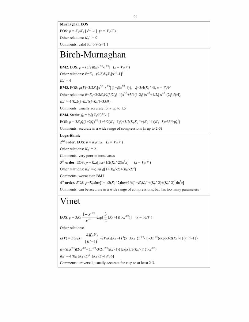
63
Murnaghan EOS
EOS: p = K0/K0’[xK0’ -1] (x = V0/V )
Other relations: K0’’ = 0
Comments: valid for 0.9<x<1.1
Birch-Murnaghan BM2. EOS: p = (3/2)K0[x7/3-x5/3] (x = V0/V )
Other relations: E=E0+ (9/8)K0V0[x2/3-1]2
K0’ = 4
BM3. EOS: p(V)=3/2K0[x7/3-x5/3]{1+ξ(x2/3-1)}, ξ=3/4(K0’-4), x = V0/V
Other relations: E=E0+3/2K0V0[3/2(ξ -1)x2/3+3/4(1-2ξ )x4/3+1/2ξ x6/3-(2ξ-3)/4],
K0’’=-1/K0{(3-K0’)(4-K0’)+35/9}
Comments: usually accurate for x up to 1.5
BM4. Strain: fE = ½[(V0/V)2/3-1]
EOS: p = 3K0fE(1+2fE)5/2{1+3/2(K0’-4)fE+3/2(K0K0’’+(K0’-4)(K0’-3)+35/9)fE2}
Comments: accurate in a wide range of compressions (x up to 2-3)
Logarithmic
2nd order. EOS: p = K0xlnx (x = V0/V )
Other relations: K0’ = 2
Comments: very poor in most cases
3rd order. EOS: p = K0x[lnx+1/2(K0’-2)ln2x] (x = V0/V )
Other relations: K0’’=-(1/K0)[1+(K0’-2)+(K0’-2)2]
Comments: worse than BM3
4th order. EOS: p=K0xlnx[1+1/2(K0’-2)lnx+1/6(1+K0K0’’+(K0’-2)+(K0’-2)2)ln2x]
Comments: can be accurate in a wide range of compressions, but has too many parameters
Vinet EOS: p = 3K0 3/2
3/11−
−−x
xexp[
23
(K0’-1)(1-x-1/3)] (x = V0/V )
Other relations:
E(V) = E(V0) + 2
00
)1'(4
−KVK
-2V0K0(K0’-1)-2(5+3K0’{x-1/3-1}-3x-1/3)exp(-3/2(K0’-1){x-1/3–1})
K=(K0x2/3)[2-x-1/3+{x-1/3-3/2x-2/3(K0’-1)}]exp(3/2(K0’-1){1-x-1/3}
K0’’=-1/K0[(K0’/2)2+(K0’/2)-19/36]
Comments: universal, usually accurate for x up to at least 2-3.

64
Table 3-2. Analytical equations of state fitted to theoretical p-V data on periclase (MgO). Murnaghan, Birch-Murnaghan (2nd and 3rd order), logarithmic (3rd-order) and Vinet (3rd-order) EOS are listed. Zero-pressure volume V0 was fixed at the theoretical value 77.64 Å3. These data were obtained by pseudopotential plane wave calculations within the generalised gradient approximation (GGA). This table shows EOS parameters obtained for a pressure range 0-pmax with N data points. The last row gives independent calculations based on the elastic constants tensor at several pressures. The table shows that: 1)At small compressions, all EOS formulations become equivalent, 2)Only Vinet and BM3 give consistent parameters in the whole pressure range, 3) K0’ crtically depends on the EOS used – again, BM3 and Vinet give the best results.
pmax (N) MUR BM2
(K0’=4
)
BM3 Logarithmic
third-order
Vinet
K0 K0’ K0 K0 K0’ K0 K0’ K0 K0’
165 GPa (12) 159.18 3.588 158.53 151.66 4.213 138.42 5.594 146.61 4.653
150 GPa (11) 158.66 3.605 158.13 151.79 4.208 140.02 5.477 147.25 4.624
105 GPa (8) 156.55 3.688 156.86 151.74 4.210 144.16 5.157 148.75 4.545
60 GPa (5) 154.70 3.788 155.29 152.12 4.186 148.43 4.781 150.67 4.416
30 GPa (3) 154.03 3.846 154.13 152.96 4.110 151.32 4.448 152.41 4.246
0 GPa K0=153.23 ; K0’= 4.2±0.1 (from elastic constants)
Since both K’ and γ come from anharmonic interactions, an intriguing possibility
arises to establish a general relation between these parameters. This possibility was
widely discussed since 1939, when J. Slater suggested the first solution of the
problem:
γs = 21 K’ –
61 (3.8.23)
Later approaches resulted in very similar equations, the difference being in the value
of the constant subtracted from ½ K’: 1/2, 5/6, or 0.95. If any of the relations of the
type (3.8.23) were accurate, it would greatly simplify the construction of thermal
EOS. Although some linear correlation between γ and K’ does exist, the correlation
is too poor to be useful (Wallace, 1998). Vočadlo et al. (2000) have examined all
approximate theories of this kind (for more details see Poirier, 2000), and confirmed
the conclusion of Wallace (1998). Vočadlo et al. (2000) also found that pressure
dependence of K’ critically depends on which analytical EOS formulation is used.
3.9. EOS, internal strain, and phase transitions.
All the EOSs discussed in the previous section were based on the assumption that
crystal structures compress uniformly, and there is no relaxation of the unit cell
shape or atomic relaxation. For some solids (e.g., MgO) this is definitely true: there

65
are no internal degrees of freedom, and the unit cell shape is fixed by symmetry. For
most crystals and all glasses, however, this is an approximation, sometimes crude.
Effects of atomic relaxation (or, internal strain) lead to renormalized values of the
EOS parameters within the fitting range – extrapolations outside this range can
become risky. As emphasized by Angel and Ross (1996), all the classical EOSs are
less successful for crystals with internal degrees of freedom. These EOSs perform
particularly poorly in the vicinity of phase transitions.
Here I propose a simplified static model taking atomic relaxation into account and
resulting in a simple additive correction. Lattice strains and thermal effects (ignored
in the present model) can be systematically included in a similar way. Homogeneous
compression leads to a configuration with atoms generally off their equilibrium
positions. I denote these displacements Qi to emphasize that they can be expressed
via specific mode eigenvectors. Denoting the energy of the crystal without atomic
relaxation as E0, in the lowest order (i.e., in the harmonic approximation) the energy
E with positional relaxation will be:
E = E0 – ½∑i
ki Qi2 ,
where k is the force constant. Recalling that for the static pressure p = -(VE
∂∂ ) we find
p(V) = -(VE
∂∂ 0 ) + ½ Σ(
VQk
∂∂ )( 2
ii ) =
= punrelaxed(V) + ΣkiQi( VQ
∂∂ i ) + ½ΣQi
2(Vk
∂∂ i ) , (3.9.1)
where punrelaxed is the pressure corresponding to the homogeneous compression.
To advance further, we need to introduce some approximations. First, let us
represent Q as a linear function of volume and take the reference Qi=0 at V=V0.
Then,
Qi = -ai(V-V0) (3.9.2)
The volume derivative of the force constant k is related to the Grüneisen
parameter, and we can write:
ki= k0i(V/V0) iγ2 (3.9.3)
(Vk
∂∂ i
)T = -2γik0i/V (3.9.4)
Substituting (3.9.2)-(3.9.4) into (3.9.1), we get:
p(V) = punrelaxed(V) + Σai2k0i[(V/V0) i2γ (V-V0) - γi/V(V-V0)2] (3.9.5)

66
or, neglecting the volume dependence of the force constant, a simplified formula:
p(V) = punrelaxed(V) +Σai2k0i(V-V0) (3.9.6)
The term punrelaxed(V) is well described by the conventional EOSs, e.g., Vinet EOS,
whereas the total EOS is not necessarily so (see below). The bulk modulus K=-
V(Vp
∂∂ )T is always lowered by the relaxation effects, in the simplest approximation
(3.9.6):
K(V) = Kunrelaxed(V) - Σai2k0iV , (3.9.7)
whereas K’ is predicted to increase:
K’(V) = K’unrelaxed(V) + Σai2k0iV/K = K’unrelaxed(V) + (δKunrelaxed(V))/K(V) (3.9.8)
This simple model explains qualitatively correctly the real effects of internal
strain. Complex structures are usually relatively ‘soft’ and usually have large K0’
(often significantly exceeding ‘normal’ K0’=4), in agreement with the prediction
(3.9.8). E.g., quartz SiO2, despite consisting of extremely rigid SiO2 tetrahedra, has a
very low bulk modulus K0 = 37.12 GPa and high K0’=5.99 (Angel et al., 1997). This
is because the structure is very flexible due to relaxation of the internal degrees of
freedom. Perhaps, the highest known K0’=13 was found in amphibole grunerite
(Zhang et al., 1992), whose structure has very many degrees of freedom.
Some new ideas spring from two series of calculations on sillimanite, Al2SiO5.
Compression behaviour of this mineral is very interesting, and will be considered in
detail in Chapter 9. Calculations were based on density functional theory within the
generalised gradient approximation (GGA: Wang & Perdew, 1991); for more details
see Chapters 5 and 9. In one series of calculations, all structural parameters were
optimised to give the minimum-enthalpy structures for a number of pressures. This
gives the correct EOS comparable to experiment; all effects of internal strains are
included in this EOS. In the other series, I took the optimised zero-pressure structure,
and calculated pressure, which would result from a simple isotropic scaling of the
lattice (without atomic relaxation) at several volumes. This gives the unrelaxed EOS.
The BM3 EOS parameters fitted to the p(V) data are V0 = 339.57 A3 (fixed), K0=
199.7 GPa (160 GPa), K0’= 4.0 (2.7) for unrelaxed (relaxed) equations of state. In
agreement with the prediction (3.9.7), the bulk modulus is lowered by relaxation. In
the unrelaxed structure, fitting results in K0’= 4.0 typical of crystals without internal
degrees of freedom (e.g., close-packed oxides and metals). For the relaxed EOS K0’=
2.7, but in fitting in a narrower pressure range, up to 15 GPa, K0’=3.7 results. At
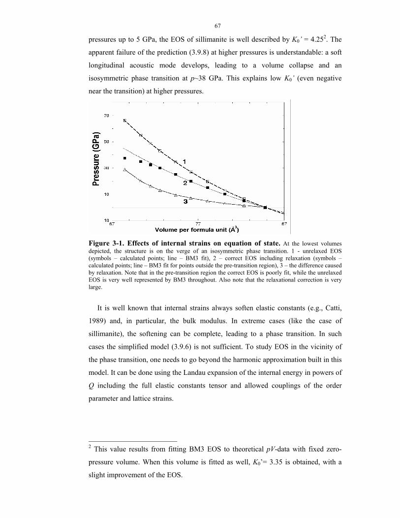
67
pressures up to 5 GPa, the EOS of sillimanite is well described by K0’ = 4.252. The
apparent failure of the prediction (3.9.8) at higher pressures is understandable: a soft
longitudinal acoustic mode develops, leading to a volume collapse and an
isosymmetric phase transition at p~38 GPa. This explains low K0’ (even negative
near the transition) at higher pressures.
Figure 3-1. Effects of internal strains on equation of state. At the lowest volumes depicted, the structure is on the verge of an isosymmetric phase transition. 1 - unrelaxed EOS (symbols – calculated points; line – BM3 fit), 2 – correct EOS including relaxation (symbols – calculated points; line – BM3 fit for points outside the pre-transition region), 3 – the difference caused by relaxation. Note that in the pre-transition region the correct EOS is poorly fit, while the unrelaxed EOS is very well represented by BM3 throughout. Also note that the relaxational correction is very large.
It is well known that internal strains always soften elastic constants (e.g., Catti,
1989) and, in particular, the bulk modulus. In extreme cases (like the case of
sillimanite), the softening can be complete, leading to a phase transition. In such
cases the simplified model (3.9.6) is not sufficient. To study EOS in the vicinity of
the phase transition, one needs to go beyond the harmonic approximation built in this
model. It can be done using the Landau expansion of the internal energy in powers of
Q including the full elastic constants tensor and allowed couplings of the order
parameter and lattice strains.
2 This value results from fitting BM3 EOS to theoretical pV-data with fixed zero-
pressure volume. When this volume is fitted as well, K0’= 3.35 is obtained, with a
slight improvement of the EOS.

68
3.10. Elastic constants.
The importance of elastic constants for the Earth sciences springs from the fact
that most of the information about the deep Earth is obtained seismologically, by
measuring the velocities of seismic waves passing through the Earth. Seismic wave
velocities, in their turn, are related to the bulk and shear moduli of the Earth-forming
rocks and minerals forming these rocks. Acoustic anisotropy of the Earth, also
measurable seismologically, is related to the elastic anisotropy of the Earth-forming
minerals and the degree of their alignement caused, e.g., by convective flow.
Knowing the full elastic constants tensors of Earth-forming minerals at relevant p-T-
conditions, it is straightforward to calculate seismic wave velocities and estimate
their anisotropy in the Earth. A number of excellent books and reviews exist; I would
emphasize Nye (1998), Sirotin & Shaskolskaya (1975), Wallace (1998), Alexandrov
& Prodaivoda (1993), Born & Huang (1954), Belikov et al. (1970), Barron & Klein
(1965), Fedorov (1968).
Elastic constants characterise the ability of a material to deform under any small
stresses. They can be described by a fourth-rank tensor Cijkl, relating the second-rank
stress tensor σij to the (also second-rank) strain tensor ekl via the generalised Hooke’s
law:
σij = Cijklekl , (3.10.1)
where multiplication follows the rules of tensor multiplication (see Nye, 1998).
Equation (3.10.1) can be simplified using the Voigt notation (Nye, 1998), which
represents the fourth-rank tensor Cijkl by a square 6*6 matrix Cmn. In these notations,
indices ‘11’, ‘22’, ‘33’, ‘12’, ’13’, ‘23’ are represented by only one symbol – 1, 2, 3,
6, 5, and 4, respectively. These notations significantly simplify all equations. So we
write instead of (3.10.1):
σi = Cijej (3.10.2)
Note that infinitesimal strains are being used; in this limit all definitions of strain
(e.g., Eulerian, Lagrangian, Hencky, etc.) become equivalent. Under a small strain,
the lattice vectors matrix aij’ of the strained crystal is obtained from the old lattice
matrix aij0 and the strain tensor eij using the relation:
aij’ = (δij+eij)aij0 . (3.10.3)
In the original tensor notation and in the Voigt notation (Nye, 1998), the (δij+eij)
matrix is represented as follows:

69
++
+
332313
232212
131211
11
1
eeeeeeeee
=
+++
++
345
426
561
12/2/2/12/2/2/1
eeeeeeeee
(3.10.4)
Voigt notation allows one to write elastic constants conveniently as a symmetric
6*6 matrix. Voigt notation is adequate for most situations; for some cases, e.g., for a
general transformation of the coordinate system, only the original fourth-rank tensor
representation can be used to derive the transformed elastic constants.
The number of components of a fourth-rank tensor is 81; Voigt notation reduces
this to 36. The thermodynamic equality Cij=Cji makes the 6*6 matrix of elastic
constants symmetric relative to its main diagonal. This reduces the number of
independent elastic constants to the well-known maximum number: 21, possessed by
triclinic crystals. Symmetry results in further reductions of this number: 13 for
monoclinic, 9 for orthorhombic, 6 or 7 (depending on the point group symmetry) for
trigonal and tetragonal, 5 for hexagonal, and 3 for cubic crystals; for isotropic
(amorphous) solids there are only 2 independent elastic constants. Elastic constants
and their anisotropy are closely related to crystal structures. E.g., for andalusite and
sillimanite (Al2SiO5) this relation was clearly demonstrated by Vaughan & Weidner
(1978).
One can define the inverse tensor Sijkl (or, in Voigt notations, Sij 3), often called the
elastic compliance tensor:
{Sijkl} = {Cijkl}-1 or {Sij} = {Cij}-1 (3.10.5)
For an orthorhombic crystal, this matrix inversion leads to the following explicit
relations between Cij and Sij (Belikov et al., 1970):
S11 = (C22C33 - C223)/D
S22 = (C11C33 - C213)/D
S33 = (C11C22 - C212)/D
S44 = 1/C44
S55 = 1/C55
S66 = 1/C66
S12 = - (C12C33 - C13C23)/D
S13 = (C12C23 - C13C22)/D
3 Note that in Voigt notation Cijkl = Cmn, but Sijkl = Smn only when m and n = 1,2, or 3;
when either m or n = 4,5, or 6: 2Sijkl = Smn; when both m and n = 4,5, or 6: 4Sijkl = Smn
(Nye, 1998).
70
S23 = - (C11C23 - C13C12)/D , (3.10.6)
where D = C11C22C33 + 2C12C13C23 - C223C11 - C2
12C33 - C213C22 . Relations (3.10.6)
are automatically valid for tetragonal and cubic crystals.
The Sij tensor can be defined via the generalised Hooke’s law in its equivalent
formulation:
ei = Sijσj (3.10.7)
Linear compressibilities can be easily derived from the Sij tensor. Full expressions
for an arbitrary direction in a triclinic crystal can be found in Nye (1998); along the
coordinate axes linear compressibilities are:
sx = - T) (1pa
a ∂∂ = ∑
=
3
11
jjS = S11 + S12 + S13
sy = - T) (1pb
b ∂∂ = ∑
=
3
12
jjS = S22 + S12 + S23
sz = - T) (1pc
c ∂∂ = ∑
=
3
13
jjS = S33 + S13 + S23 , (3.10.8)
where a, b, c are linear dimensions along the axes of the coordinate system4. For the
bulk compressibility have:
β= - T)(1pV
V ∂∂ = sx+sy+sz = ∑∑
==
3
1
3
1 jij
jS = S11 + S22 + S33 + 2(S12 +S13 + S23), (3.10.9)
where V is the volume (e.g., unit cell volume).
The values of the elastic constants depend on the orientation of the coordinate
system. There are two particularly important invariants of the elastic constants tensor
– bulk modulus K and shear modulus G. These invariants are obtained by special
averaging of the individual elastic constants. There are several different schemes of
such averaging. Reuss averaging is based on the assumption of a homogeneous stress
throughout the crystal. This leads to the Reuss bulk modulus:
KR = {S11 + S22 + S33 + 2(S12 +S13 + S23)}-1 = β1 (3.10.10)
and shear modulus:
GR = 15{4(S11 +S22 + S33) - 4(S12 +S13 +S23) + 3(S44 +S55+ S66)}-1 (3.10.11)
4 These axes may not coincide with the lattice vectors for non-orthogonal crystal
systems. Coordinate systems used in crystal physics are always orthogonal, on the
other hand.
71
Expressions (3.10.7-3.10.11) are valid for crystals of any symmetry (Nye, 1998).
It is important to realise that it is the Reuss bulk modulus, explicitly related to
compressibility, which is used in constructing EOSs. This is also the modulus
appearing in all thermodynamic equations involving the bulk modulus.
Another popular scheme of averaging is due to Voigt. It is based on the
assumption of a spatially homogeneous strain, and leads to the following expressions
for the Voigt bulk and shear moduli:
KV = 91 {C11 + C22 + C33 + 2(C12 +C13 + C23)} (3.10.12)
GV = 151 {C11 +C22 + C33 -(C12 +C13 +C23) + 3(C44 +C55+ C66)} (3.10.13)
These equations are also general, valid for crystals of any symmetry. For an
isotropic polycrystalline aggregate Voigt moduli give upper, and Reuss moduli lower
bounds for the corresponding moduli. More accurate estimates can be obtained from
Voigt-Reuss-Hill averages:
KVRH = 1/2(KV + KR)
GVRH = 1/2(GV + GR) (3.10.14)
The most accurate results (and tighter bounds) are given by Hashin-Shtrikman
variational scheme, which is much more complicated, but leads to results similar to
the Voigt-Reuss-Hill scheme.
There are two groups of experimental methods of measurement of the elastic
constants - 1) static and low-frequency methods (based on determination of stress-
strain relations for static stresses) and 2) high-frequency, or dynamic, methods (e.g.,
ultrasonic methods, Brillouin spectroscopy, etc.). Static methods are not used
anymore, because of their poor accuracy. Experiments are very complicated and
require high-quality samples; experimental uncertainties until recently were very
large, even for high-frequency measurements often 10-15% and up to 30% in some
cases (Alexandrov & Prodaivoda, 1993). During the last decade the typical
uncertainty of high-level experiments was reduced to a few percent.
Static measurements yield isothermal elastic constants (timescale of the
experiment allows thermal equilibrium to be attained within the sample), high-
frequency measurements give adiabatic constants (Belikov et al., 1970). The
difference is entirely due to anharmonic effects (see below) and vanishes at 0 K.
Adiabatic Cij are larger, usually by a few percent. The following thermodynamic
equation gives the difference in terms of thermal pressure tensor bij (Wallace, 1998):

72
CijklS = Cijkl
T + (TV/CV)bijbkl , (3.10.15)
where bij=(∂σij/∂T)V is related to the thermal expansion tensor. Equation (3.10.13)
implies for the bulk moduli:
KS = KT(1+ αγT) = KT(1+α2KTV/CV), [compare with (3.4.1)] (3.10.16)
where α and γ are the thermal expansion and Grüneisen parameter, respectively.
Adiabatic and isothermal shear moduli are strictly equal for cubic crystals and
usually practically indistinguishable for crystals of other symmetries.
Acoustic wave velocities measured in seismological experiments and ultrasonic
determinations of elastic constants are related to the adiabatic elastic constants.
Isothermal constants, on the other hand, are related to the compressibility and EOS.
The general equation for the calculation of velocities of acoustic waves with an
arbitrary propagation direction, the Christoffel equation (Sirotin & Shaskolskaya,
1975), is:
CijklSmjmkpl = ρv2pi , (3.10.17)
where p is the polarisation vector of the wave (of unit length), m unit vector parallel
to the wave vector, and ρ the density of the crystal. It can be also represented in a
form of a secular equation:
det||CijklSmjmk - ρv2δil|| = 0 (3.10.18)
There are 3 acoustic modes – 1 longitudinal (or compressional) and 2 shear ones.
Their average velocities are given by famous equations (Belikov et al., 1970):
VP = ρ3
43 GK + (3.10.19)
and
VS = ρG , (3.10.20)
where the adiabatic Voigt-Reuss-Hill (or Hashin-Shtrikman) values are used for the
bulk and shear moduli.
The energy change (per unit volume) due to a deformation can be described by the
adiabatic elastic constants:
∆E/V = ½ CijklSeijekl (3.10.21)
An analogous relation exists between the Helmholtz free energy and isothermal
constants:
∆F/V = ½ CijklTeijekl (3.10.22)
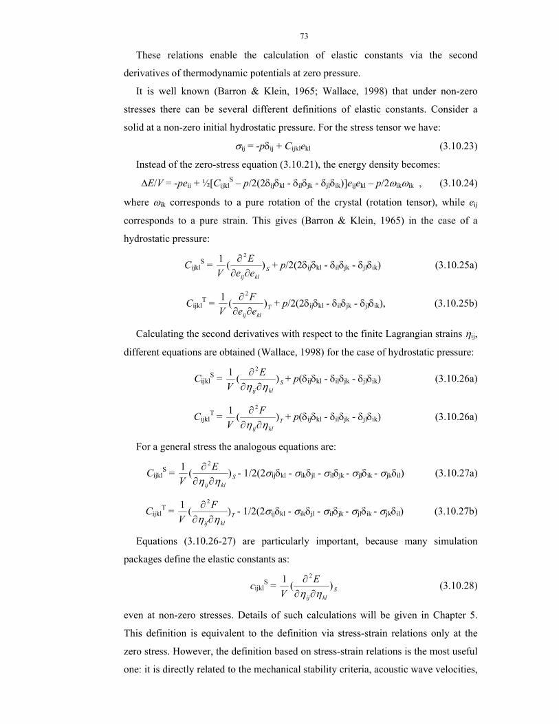
73
These relations enable the calculation of elastic constants via the second
derivatives of thermodynamic potentials at zero pressure.
It is well known (Barron & Klein, 1965; Wallace, 1998) that under non-zero
stresses there can be several different definitions of elastic constants. Consider a
solid at a non-zero initial hydrostatic pressure. For the stress tensor we have:
σij = -pδij + Cijklekl (3.10.23)
Instead of the zero-stress equation (3.10.21), the energy density becomes:
∆E/V = -peii + ½[CijklS – p/2(2δijδkl - δilδjk - δjlδik)]eijekl – p/2ωikωik , (3.10.24)
where ωik corresponds to a pure rotation of the crystal (rotation tensor), while eij
corresponds to a pure strain. This gives (Barron & Klein, 1965) in the case of a
hydrostatic pressure:
CijklS = S
klij eeE
V)(1 2
∂∂∂ + p/2(2δijδkl - δilδjk - δjlδik) (3.10.25a)
CijklT = T
klij eeF
V)(1 2
∂∂∂ + p/2(2δijδkl - δilδjk - δjlδik), (3.10.25b)
Calculating the second derivatives with respect to the finite Lagrangian strains ηij,
different equations are obtained (Wallace, 1998) for the case of hydrostatic pressure:
CijklS = S
klij
EV
)(1 2
ηη ∂∂∂ + p(δijδkl - δilδjk - δjlδik) (3.10.26a)
CijklT = T
klij
FV
)(1 2
ηη ∂∂∂ + p(δijδkl - δilδjk - δjlδik) (3.10.26a)
For a general stress the analogous equations are:
CijklS = S
klij
EV
)(1 2
ηη ∂∂∂ - 1/2(2σijδkl - σikδjl - σilδjk - σjlδik - σjkδil) (3.10.27a)
CijklT = T
klij
FV
)(1 2
ηη ∂∂∂ - 1/2(2σijδkl - σikδjl - σilδjk - σjlδik - σjkδil) (3.10.27b)
Equations (3.10.26-27) are particularly important, because many simulation
packages define the elastic constants as:
cijklS = S
klij
EV
)(1 2
ηη ∂∂∂ (3.10.28)
even at non-zero stresses. Details of such calculations will be given in Chapter 5.
This definition is equivalent to the definition via stress-strain relations only at the
zero stress. However, the definition based on stress-strain relations is the most useful
one: it is directly related to the mechanical stability criteria, acoustic wave velocities,
74
and Debye temperature. Cauchy relations, originally derived with the definition via
the energy density, can be elegantly formulated in this definition as well (see below).
Note, however, that the elastic constants Cijkl, defined from stress-strain relations,
have the full Voigt symmetry only at hydrostatic pressure. It is essential to
distinguish between different definitions of elastic constants and keep in mind the
equations (3.10.26-27). Corrections due to temperature will be discussed in the end
of this chapter.
3.11. Cauchy relations.
For crystals where all atoms occupy centrosymmetric positions, and where all
interatomic interactions are central and pairwise (i.e., depend only on the distances
between atoms, and not on angles), in the static limit Cauchy relations (Born &
Huang, 1954; but take into account eq. 3.10.25) hold:
C23-C44 = 2p ; C31-C55 = 2p ; C12-C66 = 2p
C14-C56 = 0 ; C25-C64 = 0 ; C36-C45 = 0 (3.11.1)
These relations would reduce the maximum number of independent elastic
constants to 15; however, these relations never hold exactly because there are always
non-central and many-body contributions to crystal energy. Violations of the Cauchy
relations can serve as a useful indicator of the importance of such interactions. While
for many alkali halides Cauchy relations hold reasonably well, for alkali earth
oxides, also considered as classical ionic solids, Cauchy relations are grossly
violated. This is because the free O2- ion is unstable and can exist only in the
crystalline environment due to the stabilising Madelung potential created by all
atoms in the crystal; the charge density around O2- is thus very susceptible to the
changes of structure, including strains. Consequently, interactions of the O2- ion with
any other ion depend on the volume of the crystal and location of all other ions; this
is a major source of many-body effects in ionic solids. This point of view is strongly
supported by the success of models such as PIB (Potential Induced Breathing; see
Bukowinski, 1994, and references therein), where the size of the atom depends on its
Madelung potential, in reproducing the observed Cauchy violations.
3.12. Mechanical stability.
One of the most common types of instabilities occuring in crystals is the so called
mechanical instability, when one or more elastic constants (or their special
75
combinations) tend to zero. The condition of mechanical stability is the positive
definiteness of the elastic constants matrix:
This is equivalent to positiveness of all the principal minors of this matrix
(principal minors are square sub-matrices symmetrical with respect to the main
diagonal – they are indicated by dashed lines in the scheme above). All diagonal
elastic constants Cii are principal minors, and, therefore, must be positive for all
stable crystals. Dynamical stability criteria were first suggested by Born and Huang
(1954) and are sometimes called Born conditions. In general form they are analysed
in detail in (Sirotin & Shaskolskaya, 1982; Fedorov, 1968). For crystals of different
symmetries these conditions were thoroughly analysed by (Cowley, 1976; Terhune et
al., 1985). Mechanical stability criteria for crystals under stress must employ the Cij
derived from the stress-strain relations (Wang et al., 1993; 1995; Karki, 1997).
Violation of any of the mechanical stability conditions leads to softening of an
acoustic mode in the vicinity of the Γ-point, inducing a ferroelastic phase transition.
3.13. Birch’s law and effects of temperature on elastic constants.
The famous Birch’s law (Poirier, 2000) states that compressional sound velocities
depend only on the composition and density of the material:
VP= a(−
M ) + bρ, (3.13.1)
where −
M is the average atomic mass, a and b constants, ρ the density. E.g., for the
mantle materials (average atomic mass between 20 and 22):
VP = -1.87 + 3.05ρ (3.13.2)
Similar relations are true for the bulk sound velocity VΦ = ρK ; for mantle
compositions:
C11 C12 C13 C14 C15 C16
C21 C22 C23 C24 C25 C26
C31 C32 C33 C34 C35 C36
C41 C42 C43 C44 C45 C46
C51 C52 C53 C54 C55 C56
C61 C62 C63 C64 C65 C66
76
VΦ = -1.75 + 2.36ρ (3.13.3)
Birch’s law implies that for a given material at constant volume, the elastic
constants are temperature-independent. This can be accepted only as a first (strictly
harmonic) approximation. All the deviations from Birch’s law are due to
anharmonicity – we can distinguish between quasiharmonic and intrinsically
anharmonic contributions. These contributions to the bulk modulus can be
represented (Dorogokupets, 2000) as additive corrections to the zero-temperature
result:
KT(V,T) = K0 K(V) + ∆KTqha(V,T) + ∆KT
a(V,T), (3.13.4)
∆KTqha(V,T) = pth,qha(1+γ-q) - γ2TCV/V, (3.13.5)
∆KTa(V,T) = pa(1+γa-qa) , (3.13.6)
where pa = γaEa/V and qa = (V
a
lnln
∂∂ γ
)T . For the adiabatic bulk modulus due to the
relation (3.10.16):
KS(V,T) = K0 K(V) + pth,qha(1+γ-q) + pa(1+γa-qa) (3.13.7)
These results can be generalised for the individual elastic constants. For the stress
tensor we have:
σij = -pδij + C0ijklekl - γijEvib/V , (3.13.8)
where the first term represents the initial hydrostatic pressure, the second term
contribution from zero-temperature elastic constants and strain, the third term –
thermal stress. For the isothermal elastic constants we obtain in the QHA:
CTijkl(V,T) = (∂σij/∂ekl)T =
= C0ijkl(V) - 1/V2[(∂γij/∂ekl)TEvibV + (∂Evib/∂ekl)TγijV - γijEvib(∂V/∂ekl)T] (3.13.9)
Taking into account that dV = Vdeklδkl and dEvib = -(γklEvib/V - γklTCV/V)Vdekl, we
get:
CTijkl(V,T) = C0
ijkl(V) - kl
ij
e∂∂γ
Evib/V + (γklEvib/V - γklTCV/V)γij + (γijEvib/V)δkl =
= C0ijkl(V) + (γijEvib/V)[δkl+γkl-
kl
ij
ij
1e∂
∂γγ
] - γijγklTCV/V (3.13.10)
It can be shown [cf. eq. (3.10.13)] that for the shear modulus the quasiharmonic
temperature correction is zero for a cubic crystal and very small for other crystals.
This is understandable, since there is no first-order volume change associated with
shear strains. The shear modulus then takes the form:
GT(V,T) = G0 K(V) + ∆Ga(V,T) , (3.13.12)
77
where ∆Ga(V,T) is the intrinsic anharmonic contriution to the shear modulus. Often
this correction is large.
Garber and Granato (1975), differentiating the free energy expressed as a sum of
mode contributions (3.2.6) over the whole Brillouin zone:
F = Est + 21 ∑
k,ihωik + ∑
k,B
ik Tln[1-exp(
TkB
iω kh− )] , (3.13.13)
obtained the following result:
Vklij
FV
)(1 2
ηη ∂∂∂ = V
klij
EV
)(1 st2
ηη ∂∂∂ + ∑
k,[1
iV(γ ki
ij γ kikl -
kl
ij
ηγ
∂
∂)Evib,ik - γ ki
ij γ kikl CV,ikT] (3.13.14)
The next chapter gives an introduction to phase transitions. Some of the most
important theoretical results and general ideas will be presented there. Crystal
thermodynamics and elasticity, considered in this chapter, are among the key areas of
interest in the study of phase transitions.
78
Chapter 4. Phase transitions. The study of phase transitions is of a central importance to modern
crystallography, condensed matter physics and chemistry. Spectacular evolution of
facts, ideas and theories, and technological applications of phase transitions during
the last 50 years has made phase transitions one of the most popular topics in
condensed matter physics. Much attention was recently paid to metastable
phenomena, due to their practical importance and poor theoretical understanding.
Phase transitions are a major factor determining the seismic structure of the Earth
(see Chapter 2) and thus play a special role in geophysics. In this Chapter I give a
brief review of the theory and classification of phase transitions. Various aspects of
phase transitions will be seen throughout this thesis, especially in Chapter 9.
4.1. Classifications of phase transitions.
Perhaps the first sound classification of phase transitions was proposed by
Ehrenfest in 1933 (for a detailed historical and scientific discussion see Jaeger,
1998). This purely thermodynamic classification distinguished between first-,
second-, and higher-order phase transitions. For the first-order transitions the first
derivatives of the free energy with respect to p and T (i.e., volume and entropy) are
discontinuous at the transition point; for second-order transitions the second
derivatives (compressibility and thermal expansion) are discontinuous, and so forth.
Third- and higher-order transitions, though theoretically possible, so far have never
been reported. More modern variants of the Ehrenfest classification distinguish only
between ‘first-order’ and ‘continuous’ (i.e., all higher-order) transitions. In some
cases, the order of the same phase transition is different at different p-T conditions.
As we will see, isosymmetric transitions must be first order, but become completely
continuous (infinite-order) transitions at and above the critical temperature. Some
transitions change from first- to second-order; the crossover point is called the
tricritical point. Among the examples of systems with tricritical crossover are NH4Cl
(Garland & Weiner, 1971), zone-centre cubic-tetragonal transition in BaTiO3
perovskite, possibly the transition from calcite to metastable calcite (II) in CaCO3
(see Hatch & Merrill, 1981), and, possibly, the α-β transition in quartz (SiO2). For
example, the order-disorder transition in NH4Cl from a phase with a complete
orientational disordering of the NH4-group (Pm−
3 m) to an ordered phase (P4−
3 m) is

79
first-order at 1 atm and 242 K, but becomes second-order at the tricritical point, 0.15
GPa and 256 K.
Therefore, the order of the transition is not something fundamentally inherent to
the transition. The Ehrenfest classification, however useful (it is still being widely
used as a standard classification), attempts to describe only thermodynamics of phase
transitions without linking it to any structural mechanisms or symmetry aspects of
transitions. However, it is the structure and symmetry relations between the phases,
which are the most fundamental invariant characteristic of any phase transition.
The first structural classification was due to Buerger (1961), who, instead of
thermodynamics, used the intuitive language of structural schemes. First of all, he
distinguished two main types of phase transitions – those with and without changes
of the first coordination number. Each of these types was further classified into
reconstructive (i.e., requiring formation/breaking of bonds), displacive, order-
disorder, electronic, etc. transitions. Displacive phase transitions are accompanied by
small atomic displacements (hence the name), which usually destroy some elements
of symmetry. These displacement patterns are determined by the eigenvectors of one
or more normal modes – the so-called soft modes. Order-disorder transitions occur
between a low-temperature structurally ordered (e.g., having positional order in
cation distribution and orientational order of atomic groups) and a high-temperature
disordered phase. Electronic transitions are accompanied by a change of the
electronic or magnetic structure and/or valence state of atoms in the structure; the
structure type may or may not change in this process. Reconstructive phase
transitions, by Buerger’s definition, involve breaking/formation of at least some
bonds. These transitions are always first order, involve a latent heat, and require an
activation energy for bond breaking. In systems with typical reconstructive
transitions, due to kinetics, phases can exist as metastable outside their stability
fields. Order-disorder and displacive transitions can in principle be of any order. A
modification of Buerger’s classification was proposed by Urusov (1987).
The beauty of the Buerger classification is that, even though based on purely
structural considerations, it naturally gives some insight into thermodynamics and
kinetics of phase transitions. Its weakness is in the absence of a precisely formulated
quantitative basis. Formation/breaking of bonds is one of the main criteria. However,
there is no rigorous physical definition of a chemical bond in a many-atom system.
In many practical cases it is very difficult to say whether or not two atoms in a given
structure are linked by a bond or determine the coordination number of an atom in a
80
crystal5. This question is still an area of active research. In addition to this
fundamental weakness, Buerger’s classification does not discuss symmetry aspects
of transitions.
It was first realised by L.D. Landau in 1937 (see Landau & Lifshitz, 1980) that
often there are symmetry relations between the old and new phases. Landau has
shown that for a second-order transition the two phases must be structurally related,
and their symmetry groups must conform to certain group-subgroup relations.
Symmetry plays a fundamental role in phase transitions, and better classifications
must consider it; such a classification is proposed below6. Before considering this
new classification, I describe some of the main theoretical ideas related to phase
transitions.
4.2. Theoretical framework.
4.2.1. First-order phase transitions.
Equilibrium first-order phase transitions always involve activation, which
substantially complicates their kinetics. The major factors determining the kinetics
are defects, surface effects, and external fields. Polymorphs of Al2SiO5 (minerals
kyanite, andalusite, and sillimanite, see Kerrick, 1990) are a classical example. All
the transitions between these minerals are first-order reconstructive and require
substantial activation energies to proceed; therefore, all the three minerals can
coexist at not very high temperatures for millions of years in nature. A very
interesting example is given by the HgI2 polymorphs (Hostettler et al., 2001). At
p<10 GPa and T<600 K, there are nine polymorphs in this system! Crystallisation
from solution (which contains HgI2 molecules) first produces a metastable yellow
form, whose structure consists of linear HgI2 molecules, and only then metastable
orange (containing supertetrahedra [Hg4I10]) and stable red (containing HgI4
tetrahedra) forms. Metastable yellow and orange crystals begin to transform into the
red phase when touched by a needle. Defects thus introduced serve as nucleation
centres of the stable phase. The orange phase is in fact represented by three distinct,
but similar, structures, which can transform into one another. This system is a good
example of the Ostwald rule, which states that often crystallisation produces a
metastable phase, which transforms into the stable one via a sequence of metastable
5 There have been many attempts to derive structural criteria for the determination of coordination numbers and bond graphs. One of the latest attempts was due to Bader (1990). 6 Another classification based on symmetry was propsed by Christy (1993).

81
phases. At high temperatures, another yellow molecular form is stable (it can
crystallise from the vapour). At 1.3 GPa a new phase is formed, where Hg atoms are
five-coordinate. A somewhat similar kinetical behaviour was reported for Dimethyl
3,6-Dichloro-2,5-dihydroxyterephtalate (Richardson et al., 1990). For that
compound, transformation kinetics and actual transition temperatures were found to
depend on such factors as crystal size, degree of perfection, types of defects, and
heating rate. Again, defects play the role of nucleation sites for the new phase.
Thermodynamics of first order transitions are based on the Clapeyron relation:
dp/dT =∆S/∆V, (4.2.1.1)
where ∆S and ∆V are the entropy and volume differences, respectively, between the
phases. Using (4.2.1.1) one can calculate the slopes of the equilibrium lines of phase
coexistence. This relation is valid only for first-order transitions, because for
continuous transitions both ∆V and ∆S are equal to zero. The transition temperatures
and pressures can be found from accurate atomistic (e.g., Parker & Price, 1989:
magnesium silicates) or quantum-mechanical total energy calculations (e.g., Oganov
& Brodholt, 2000: aluminium silicates), but there is no simple analytical theory.
Only when the two phases are structurally similar can one apply approximate
analytical theories, such as Landau theory (which was initially devised to study
second-order phase transitions).
A relation, analogous to (4.2.1.1), for second-order transitions was derived by
Ehrenfest:
dp/dT=∆CP/TV∆α , (4.2.1.2)
where ∆CP and ∆α are the jumps of the heat capacity and thermal expansion at the
transition. However, precise experiments, computer simulations, and accurate
theories indicate a qualitatively different behaviour of the heat capacity – instead of
having a finite jump, it logarithmically diverges to infinity on both sides of the
transition. This ‘λ-behaviour’ invalidates the Ehrenfest relation.
4.2.2. Landau theory of first-and second-order transitions.
When the structural changes occurring upon transition are rather small, i.e. the
two phases are structurally related, it is usually possible to define an order parameter
(or several order parameters), whose continuous change describes all the
intermediate structures on the transition pathway. The order parameter Q takes the

82
value, which would minimise the free energy F(Q) at given p-T conditions. The
simplest expression for the free energy is the Landau potential:
F(Q)=F0 + 21 A(T-TC)Q2 +
31 BQ3 +
41 CQ4+… , (4.2.2.2)
where TC is the critical temperature, and F0 the free energy of the phase with Q=0
(e.g., high-temperature high-symmetry disordered phase). Landau’s assumption that
the second term of (4.2.2.2) is simply proportional to (T-TC) was analysed and
justified mathematically within the mean-field approach by Sposito (1974). The
entropy as a function of the order parameter is simply S(Q) = -∂F(Q)/∂T = S0 -
21 AQ2. This dependence of the entropy on the order parameter is most appropriate
for displacive phase transitions7. The internal energy is then E(Q) = E0 –
21 ATCQ2+
31 BQ3+
41 CQ4+… In the case A>0, B>0, C>0, this corresponds to a
double-well potential E(Q) 8. For second-order transitions the odd-order terms in
(4.2.2.2) must be zero (e.g., B=0), making the double well symmetric9. When B≠0,
the double well is asymmetric, and the transition is first order. First-order transitions
can also appear when C<0 (even if B=0), which requires a positive term 61 DQ6 to
prevent the system from collapse.
Consider a second-order transition:
F(Q) = F0 + 21 A(T-TC)Q2 +
41 CQ4+…. (4.2.2.3)
One can observe that at the transition point (T=TC, Q=0) the second derivative of F
with respect to Q: 2
2 )(Q
QF∂
∂ = A(T-TC)+3CQ2+… changes its sign: it is negative
below TC and positive above TC. For displacive phase transitions, where the order
parameter Q corresponds to a particular atomic displacement, this second derivative
corresponds to the squared frequency of a normal vibrational mode10. Its frequency ω
is imaginary (i.e., 2
2 )(Q
QF∂
∂ ~ ω2 is negative) in the high-symmetry phase below TC,
7 For order-disorder transitions the entropy is more accurately expressed as S(Q)=S0-R[(1+Q)ln(1+Q)+(1-Q)ln(1-Q)]. 8 More than two minima can exist for higher-order polynomials (4.2.2.2). 9 This is only one of the necessary conditions. Other conditions were formulated by Birman (1966) by using group theory. All these conditions are necessary, but not sufficient. 10 And Q is its normal coordinate (see Chapter 5).
83
leading to a spontaneous distortion into a low-symmetry phase11. Above TC, due to
intrinsic anharmonic effects, this frequency becomes positive, stabilising the high-
symmetry phase against distortions (see Dove, 1993, 1997). It is said that the low-
symmetry phase is formed by condensation of a soft mode at T=TC. Experiments do
show that at the transition point one of the vibrational frequencies becomes
practically zero for second-order transitions (e.g., in SrTiO3 at 110 K – see Dove,
1993).
Transitions, where the soft mode is an optic mode associated with creation of a
spontaneous electric dipole in the low-symmetry phase, are called ferroelectric.
When the soft mode is an acoustic mode at the Brillouin zone centre, some of the
elastic constants become zero at the transition point, and a spontaneous lattice strain
is generated; such transitions are termed ferroelastic (see Salje, 1993)12. For
ferromagnetic transitions a net magnetic moment is generated on transition from a
high-temperature paramagnetic phase to a low-temperature ferromagnetic phase.
For first-order transitions, complete mode softening does not occur at T=TC. For
these transitions a hysteresis in temperature is observed, and mode softening can
occur at the ends of the hysteresis region. All these features are correctly predicted
by Landau theory.
The power of Landau theory comes from the fact that simple symmetry
considerations allow one to find which of the coefficients B, C,… must be zero, and
therefore (see below) which is the order of the transition and how many terms must
be included in the Landau potential, including possible couplings to the strains (see
below). Second-order phase transitions, corresponding to a symmetrical double-well
potential E(Q), are always characterised by group-subgroup relations: the symmetry
group of one (often called ‘ordered’, usually low-temperature) phase is a subgroup of
the symmetry group of the other (‘disordered’, usually high-temperature) phase. The
two symmetrically equivalent minima then correspond to the same ordered phase,
and can be considered as ‘twin domains’, related by a symmetry element present in
the disordered phase, but absent in the ordered one (Fig. 4-1).
The potential (4.2.2.2) is often complicated by the coupling of the order parameter
to lattice strains. In such cases the potential will be:
11 This is the so-called dynamical instability. The soft wavevector k determines the modulation of the structure; the mode eigenvectors determine vectors of atomic displacements leading to the low-symmetry phase. 12 This important particular case of dynamical instability is called mechanical instability (see Chapter 3).
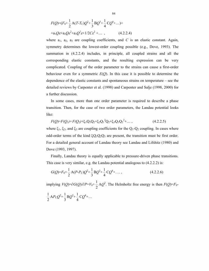
84
F(Q)=(F0+ 21 A(T-TC)Q2+
31 BQ3+
41 CQ4+…)+
+a1Qε+a2Qε2+a3Q2ε+1/2Cε2 +… , (4.2.2.4)
where a1, a2, a3 are coupling coefficients, and C is an elastic constant. Again,
symmetry determines the lowest-order coupling possible (e.g., Dove, 1993). The
summation in (4.2.2.4) includes, in principle, all coupled strains and all the
corresponding elastic constants, and the resulting expression can be very
complicated. Coupling of the order parameter to the strains can cause a first-order
behaviour even for a symmetric E(Q). In this case it is possible to determine the
dependence of the elastic constants and spontaneous strains on temperature – see the
detailed reviews by Carpenter et al. (1998) and Carpenter and Salje (1998, 2000) for
a further discussion.
In some cases, more than one order parameter is required to describe a phase
transition. Then, for the case of two order parameters, the Landau potential looks
like:
F(Q)=F(Q1)+F(Q2)+ξ1Q1Q2+ξ2Q12Q2+ξ3Q1Q2
2+… , (4.2.2.5)
where ξ1, ξ2, and ξ3 are coupling coefficients for the Q1-Q2 coupling. In cases where
odd-order terms of the kind ξQ1Q2Q3 are present, the transition must be first order.
For a detailed general account of Landau theory see Landau and Lifshitz (1980) and
Dove (1993, 1997).
Finally, Landau theory is equally applicable to pressure-driven phase transitions.
This case is very similar, e.g. the Landau potential analogous to (4.2.2.2) is:
G(Q)=F0+ 21 A(P-PC)Q2+
31 BQ3+
41 CQ4+…. , (4.2.2.6)
implying V(Q)=∂G(Q)/∂P=V0+ 21 AQ2. The Helmholtz free energy is then F(Q)=F0-
21 APCQ2+
31 BQ3+
41 CQ4+…
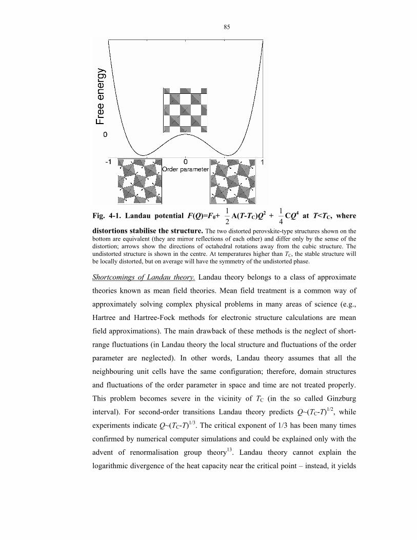
85
Fig. 4-1. Landau potential F(Q)=F0+ 21 A(T-TC)Q2 +
41 CQ4 at T<TC, where
distortions stabilise the structure. The two distorted perovskite-type structures shown on the bottom are equivalent (they are mirror reflections of each other) and differ only by the sense of the distortion; arrows show the directions of octahedral rotations away from the cubic structure. The undistorted structure is shown in the centre. At temperatures higher than TC, the stable structure will be locally distorted, but on average will have the symmetry of the undistorted phase. Shortcomings of Landau theory. Landau theory belongs to a class of approximate
theories known as mean field theories. Mean field treatment is a common way of
approximately solving complex physical problems in many areas of science (e.g.,
Hartree and Hartree-Fock methods for electronic structure calculations are mean
field approximations). The main drawback of these methods is the neglect of short-
range fluctuations (in Landau theory the local structure and fluctuations of the order
parameter are neglected). In other words, Landau theory assumes that all the
neighbouring unit cells have the same configuration; therefore, domain structures
and fluctuations of the order parameter in space and time are not treated properly.
This problem becomes severe in the vicinity of TC (in the so called Ginzburg
interval). For second-order transitions Landau theory predicts Q~(TC-T)1/2, while
experiments indicate Q~(TC-T)1/3. The critical exponent of 1/3 has been many times
confirmed by numerical computer simulations and could be explained only with the
advent of renormalisation group theory13. Landau theory cannot explain the
logarithmic divergence of the heat capacity near the critical point – instead, it yields
86
a finite jump. Finally, Landau theory does not consider quantum effects at low
temperatures. As a consequence, it does not reproduce experimentally observed
order parameter saturation at low temperatures; instead, it predicts a steady increase
of the order parameter with decreasing temperature. However, it is generally
believed that the symmetry apparatus of Landau theory is valid even where mean-
field theory breaks down.
Ginzburg-Landau theory. In 1950, V.L. Ginzburg and L.D. Landau (see Landau &
Lifshitz, 1980; Bowley & Sánchez, 1999) considered the case of an order parameter
slowly varying in space. This leads to the simplest theory beyond the mean-field.
The free energy becomes a functional of the order parameter, and an additional term
proportional to the square of the gradient of the order parameter appears:
F[Q(r)]= ∫ ∇+ rQQf d})]([21))(({ 2rr λ (4.2.2.7)
with the stiffness parameter λ>0. E.g., for a second-order transition,
F[Q(r)]= ∫ ∇++− rQbQQTTa d})]([21)(
41)()(
21{ 242
C rrr λ (4.2.2.8)
Then, Ginzburg and Landau express the order parameter as a sum of a constant term (the average order parameter) and fluctuations, which they express as a Fourier series:
Q(r) = −Q + ∑
k
krk
iQ e (4.2.2.9)
Eq. (4.2.2.7) can be re-written as:
F[Q(r)] = ∫ ∇++++−
rQfQfQQf d})]([21...'')(
21')()({ 22
11 rrr λ =
= V{ )(−Qf + ...)''(||
21 22
++∑ kfQ λk
k } (4.2.2.10)
The system is stable against all fluctuations if f ’’+λk2>0 (a more strict condition
is f ’’>0) at all Q. If there is more than one minimum, f ’’<0 at some Q. By means of
fluctuations, the system eventually reaches the state with the lower free energy.
Let us consider the case f ’’<0. In this case, the system is unstable against all
fluctuations whose wavevectors satisfy f ’’+λk2>0. Hence, the maximum unstable
wavevector is kc=λ
|''| f . The correlation length ξ is:
ξ = kc-1 =
|''| fλ (4.2.2.11)
13 In fact, experiments give mean-field critical exponents far from TC, but nearer TC there is a crossover from the mean-field to critical behaviour, where the critical exponents depart significantly from the mean-field predictions.
87
Ginzburg and Landau have proposed a criterion of the validity of Landau theory.
They defined the following value:
r(T) = Tk
f
B
3mξ , (4.2.2.12)
where fm is the difference of energies at the energy maximum and minimum. If
r(T)>1, fluctuations are not important, and Landau theory is valid. When r(T)<1,
fluctuations are essential and Landau theory is invalid; this occurs in the vicinity of
TC (this temperature region is called Ginzburg interval). Ginzburg intervals are
usually quite narrow (of the order of ~10 K).
For second-order transitions, fm = b
TTa C
4)(2 −
and
ξ = )(2 TTa C −
λ , (4.2.2.13)
Ginzburg-Landau theory emphasises the role of critical fluctuations and defines
criteria of validity of Landau theory. However, this theory is still approximate and
does not reproduce experimental critical exponents, e.g. for the correlation length
(4.2.2.13). Renormalisation group theory overcomes all these difficulties and serves
as the modern basis of the theory of critical phenomena; applications of that theory
extend well beyond the field of phase transitions and can be found in astronomy,
engineering, and geology.
4.2.3. Renormalisation group theory (RGT).
This theory goes beyond the mean-field approximation and fully treats all possible
fluctuations of the order parameter. Introductory texts on this theory can be found in
Chandler (1987), Rao and Rao (1978), and Wilson (1983); the latter reference is the
Nobel lecture of Kenneth Wilson, the main inventor of RGT. This theory is based on
repeated scaling transformations of the system and its Hamiltonian, during which
some degrees of freedom (e.g., some fluctuations of the order parameter) are
removed. At phase transitions, the system becomes scale-invariant, and the
behaviour of the system is determined by the long-wavelength fluctuations,
insensitive to the details of atomic structure.
RGT explains the famous scaling hypothesis which states that ‘the correlation
length, ξ, should be the longest and the only relevant length in explaining critical
phenomena’ (Rao & Rao, 1978). Fluctuations with the wavelength exceeding the

88
correlation length are always negligible, but itself the correlation length diverges at
the critical point to infinity as TC - T-ν (Ginzburg-Landau theory gives ν=1/2 – see
(4.2.2.13), but experiment indicates ν=2/3). The exponent ν is not sensitive to the
type of interatomic interactions, so critical phenomena in all systems (e.g., in metals,
covalent, molecular, and ionic systems, solids, liquids, and gases) must be similar
and all their critical exponents must be the same. The temperature dependence of ξ
(ξ~TC - T-ν), according to the scaling hypothesis, accounts for the major part of
the temperature dependence of all properties near the critical point; ‘physical
quantities depend on TC - T only through their dependence on ξ’ (Rao & Rao,
1978).
Describing the average order parameter Q near the critical point, we have Q~(TC -
T)β, where for 3D-systems the critical exponent β=1/2 from Landau theory or 1/3
from experiment, computer simulations, and RGT. Critical exponents depend on the
dimensionality of the system, and this is clearly demonstrated by RGT.
For example, in two dimensions, β=1/8, whereas Landau theory would always14
give β=1/2. According to the other important hypothesis, understood only with the
advent of RGT, the universality hypothesis, all critical phenomena can be classified
by the dimensionality of the system and symmetry of the order parameter, but again
not the chemical nature or structural details of the substance15. This means that
models with simplified interactions (e.g., nearest-neighbour Ising models) still give
correct critical exponents for their universality class (i.e., for all systems of the same
dimensionality having order parameters of the same symmetry).
Using RGT, it can be shown that Landau theory (like any other mean-field theory)
yields exact critical exponents for four- and higher-dimensional spaces; at the infinite
number of dimensions all other aspects of Landau theory become exact. For lower-
dimensional spaces mean-field theories become increasingly less applicable.
Finally, RGT predicts that some systems can exhibit continuous lattice melting
close to the transition point. Continuous lattice melting means that on approaching
the transition point, mean-square atomic displacements diverge as ln(TC - T), but 14 Here I consider only the second-order transitions, described by the simplest potential
F(Q)=F0+ 21
A(T-TC)Q2+41
CQ4. When other terms are included, β changes. E.g., when DQ6 term is
added, β can take values between 0.25 and 0.5 (second order transitions), 0.25 (intermediate, or tricritical, transitions), less than 0.25 (first order transitions), or larger than 0.5 (see Redfern, 2000).

89
only in one direction, that crystal lattice is destroyed, and Bragg reflections disappear
being replaced by broad diffuse scattering centred at the positions of Bragg peaks.
After passing through the transition point, the system spontaneously recrystallises
into the high-temperature phase. So far, only one example of such behaviour was
found experimentally: Na2CO3 (Harris & Dove, 1995). The necessary condition of
continuous lattice melting is that the system is 3-dimensional, and is characterised by
softening of a transverse acoustic mode in a whole plane of the reciprocal space.
4.2.4. Ising spin model.
This model is widely used to describe magnetic and atomic ordering processes in
materials. In this model, a spin +1 or –1 is associated with each lattice site,
depending on whether the magnetic moment on the site is ‘up’ or ‘down’, or whether
the atom occupying the site is of the type ‘A’ or ‘B’.
The total energy of the system is:
E = E0 – J∑ji
jiss,
- H∑i
is , (4.2.4.1)
where E0 is the reference-state energy, and J the interaction parameter between the
sites: if J<0, unlike spins prefer to group together, and there is a tendency to ordering
at low temperatures; if J>0, unmixing will occur at low temperatures. Full disorder,
although unfavourable energetically, will be stabilised by the entropy at high
temperatures. An external field H leads to a preferred orientation of the spins. The
Ising model can be analytically solved only in one and two (Onsager’s solution)
dimensions; for three dimensions it is solved numerically, usually by the Monte
Carlo method. Note that the one-dimensional Ising model exhibits no phase
transitions, and at all temperatures above 0 K yields the disordered state.
As noted above, the Ising model has found many applications in describing
atomic and magnetic ordering in crystals. Numerical simulations based on the Monte
Carlo method and Ising model yield critical exponents close to the values given by
experiments and predicted by renormalisation group theory.
Ising-like models provide an interesting route for theoretical studies of polytypism
and polysomatism. The crucial observation is the mathematical similarity between
polytypic sequences (e.g., Fig. 4-2a-c) and one-dimensional Ising models. Layers of
polytypic structures are mapped onto spin-sites of a one-dimensional Ising lattice. 15 This can be understood from the fact that critical behaviour is determined by long-wavelength fluctuations; on the other hand, chemical details are only important at short wavelengths – those
90
Including interactions between up to three nearest layers (Price, 1983), it is possible
to explain the existence of almost all the observed polytypes in spinelloid systems
(Fig. 4-2d,e) just by considering the ground-state (i.e., 0 K) energy16. Generally,
longer-period polytypes require the presence of longer-range interactions to stabilise
them.
The strength of interactions decreases with distance, which explains why long-
period polytypes are rarely found. Let us denote, following Price and Yeomans
(1984), polytypes in a Zhdanov-like manner: e.g., the sequence
…↑↑↓↓↑↑↓↓↓↑↑↓↓↑↑↓↓↓… as <2223>, or <233>. This symbol reads as follows:
two layers ‘spin-up’ are followed by 2 ‘spin-down’, then there are two ‘spin-up’, and
three ‘spin-down’ layers. The stable stacking sequences are: <∞>, <1>, <2>, <3>,
<12>, with marginal stability of longer-period phases along the boundary lines
between these major phases.
A realistic inclusion of temperature necessitates an extension of the model beyond
one dimension. The Axial Next-Nearest-Neighbour Ising (ANNNI) model (see, e.g.,
Price & Yeomans, 1984 and references therein) does this. The system is mapped
onto a 3D-Ising lattice; each lattice site represents a finite building block of the
structure. For simplicity, only the interactions between the nearest and next-nearest
layers are included; within the layers, a certain degree of disorder is allowed,
determined by the Ising-like interactions (4.2.4.1) with different (generally, much
larger and possibly anisotropic) interaction parameters J. This model reproduces the
stability of relatively long-period polytypes. In this model, they are stable due to a
competition between the internal energy and entropy, both of which are determined
by short-range interactions17. With increasing temperature, more longer-period
polytypes acquire stability fields18, and such phases as <23>, <122>, <223>, <123>,
etc., appear
comparable to bond lengths. 16 Finite-temperature behaviour cannot be studied with the one-dimensional Ising model: at non-zero temperatures the spin arrangement of this model becomes completely random. 17 This is an equilibrium picture. In many cases, long-period polytypes are metastable systems, formed during crystal growth and related to dislocations and stacking faults. 18 This implies that long-period polytypes are stabilised by the configurational entropy. This extra entropy comes from the thermal disorder within the layers. This is a very non-trivial conclusion. One must remember, however, that the ANNNI model is very crude in its way of accounting for the intralayer disorder. It also completely neglects possible lattice strains and the associated energy terms.
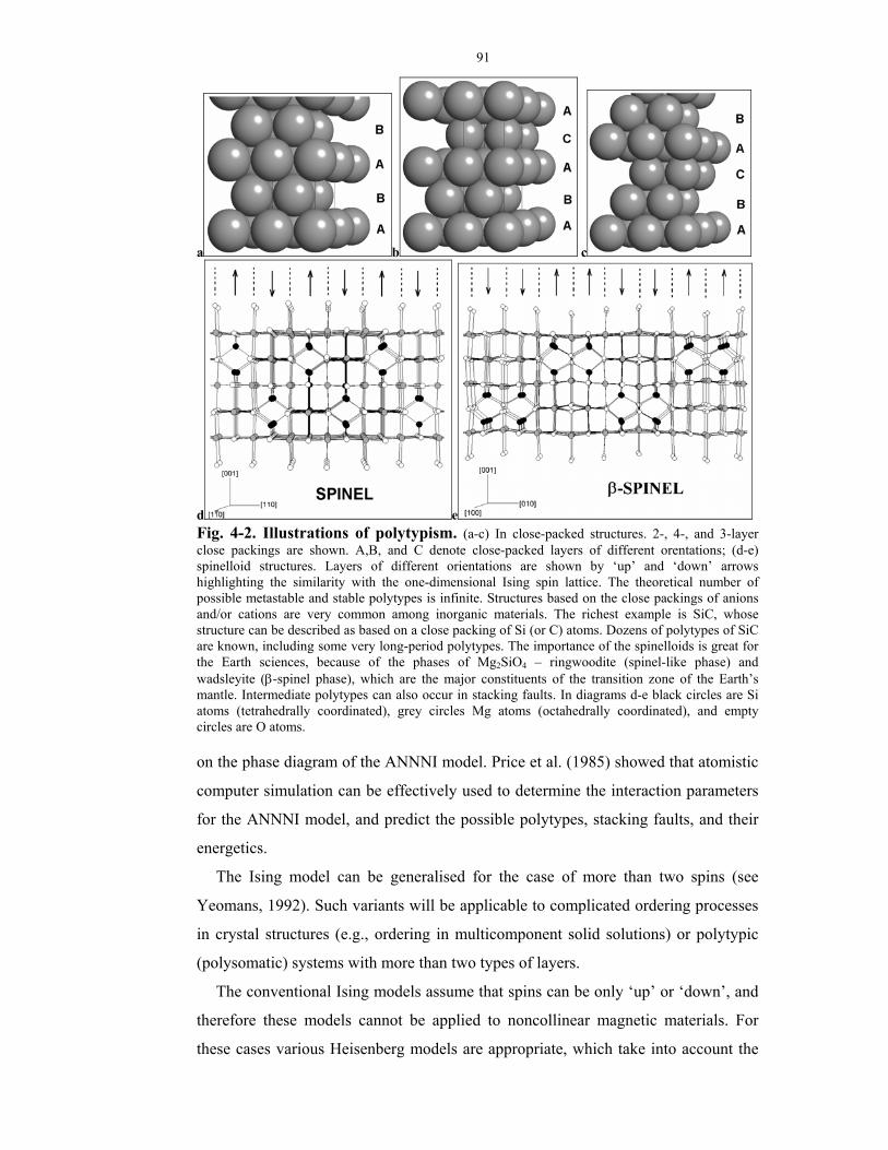
91
a b c
d e Fig. 4-2. Illustrations of polytypism. (a-c) In close-packed structures. 2-, 4-, and 3-layer close packings are shown. A,B, and C denote close-packed layers of different orentations; (d-e) spinelloid structures. Layers of different orientations are shown by ‘up’ and ‘down’ arrows highlighting the similarity with the one-dimensional Ising spin lattice. The theoretical number of possible metastable and stable polytypes is infinite. Structures based on the close packings of anions and/or cations are very common among inorganic materials. The richest example is SiC, whose structure can be described as based on a close packing of Si (or C) atoms. Dozens of polytypes of SiC are known, including some very long-period polytypes. The importance of the spinelloids is great for the Earth sciences, because of the phases of Mg2SiO4 – ringwoodite (spinel-like phase) and wadsleyite (β-spinel phase), which are the major constituents of the transition zone of the Earth’s mantle. Intermediate polytypes can also occur in stacking faults. In diagrams d-e black circles are Si atoms (tetrahedrally coordinated), grey circles Mg atoms (octahedrally coordinated), and empty circles are O atoms.
on the phase diagram of the ANNNI model. Price et al. (1985) showed that atomistic
computer simulation can be effectively used to determine the interaction parameters
for the ANNNI model, and predict the possible polytypes, stacking faults, and their
energetics.
The Ising model can be generalised for the case of more than two spins (see
Yeomans, 1992). Such variants will be applicable to complicated ordering processes
in crystal structures (e.g., ordering in multicomponent solid solutions) or polytypic
(polysomatic) systems with more than two types of layers.
The conventional Ising models assume that spins can be only ‘up’ or ‘down’, and
therefore these models cannot be applied to noncollinear magnetic materials. For
these cases various Heisenberg models are appropriate, which take into account the
92
orientations of the spins. The simplest of these models is based on the following
Hamiltonian:
E = E0 - J∑ji ,
jiss - H∑i
zsi , (4.2.4.2)
involving spin vectors si and sj. Like the Ising model had no phase transitions for
one-dimensional systems, the Heisenberg model has no phase transitions for one-
and two-dimensions systems.
4.2.5. Mean-field treatment of order-disorder phenomena.
The Bragg-Williams model is the simplest mean-field approach applicable to
ordering phenomena. The Helmholtz free energy of the alloy as a function of
temperature and order parameter is:
F=E-TS=F0-4
NzJQ2 +NkBT [(1+Q)ln(1+Q)+(1-Q)ln(1-Q)] , (4.2.5.1)
where E0 is the internal energy of the fully disordered state, N is the number of sites
where disordering occurs, the order parameter Q= XA,α-XA,β= XB,β-XB,α=2XA,α-1,
and the exchange energy J=EAA+EBB-2EAB.
The expression (4.2.5.1) is analogous to the Landau potential (4.2.2.2), and yields
the same critical exponents (e.g., Q~(TC-T)1/2 near the critical point). The Bragg-
Williams model has a phase transition even in the one-dimensional case; generally,
as for any mean-field model, the accuracy of predictions of the Bragg-Williams
model increases with the dimensionality of the system. In three dimensions this
model gives qualitatively reasonable results; however, even with accurate exchange
energies J, the predicted transition temperatures are usually a few times higher than
the experimental ones (Redfern, 2000).
Drawbacks of the Bragg-Williams model can be corrected by explicitly
considering short-range order. In the Bethe model (see Rao & Rao, 1978), apart from
the long-range order parameter Q, one or more short-range order parameters are
considered. These additional parameters describe the distribution of neighbours of
both kinds in the nearest proximity of each atom. Bethe and related models yield
critical exponents and transition temperatures, which are much more realistic than
the mean-field predictions.
4.3. New classification of phase transitions.
4.3.1. Phase transition scenarios.

93
All possible modifications of a given substance correspond to minima of the free
energy hypersurface. The global (i.e., the deepest) minimum is related to the phase
thermodynamically stable at given p-T-conditions, while local minima correspond to
metastable phases. The free energy hypersurface determines the crystal structure and
many of its properties; it also determines all possible transition states, phase
transition paths, and activation barriers. In principle, the free energy hypersurface is
a function of all coordinates of all the atoms in the system (i.e., the free energy
hypersurface is infinite-dimensional for an infinite system such as an ideal crystal).
In principle there can be an infinite number of local minima on this surface,
corresponding to an infinite number of possible metastable phases. These phases and
their properties can be simulated on the computer, but it is remarkable that only a
handful of them can be experimentally synthesised and studied.
The free energy hypersurface provides the most fundamental link between crystal
structure, thermodynamics, and kinetics of all processes. Although the hypersurface
itself is extremely complicated, we still can fruitfully exploit its concept in studying
phase transitions. Often the dimensionality of the hypersurface can be effectively
reduced, and only a finite part of the degrees of freedom (e.g., only those
corresponding to one unit cell or a supercell) considered. Mean-field theories such as
Landau theory are based on such reductions (e.g., for a system with one order
parameter, Landau theory reduces the infinite-dimensional hypersurface to a one-
dimensional function! – Fig. 4-1).
At this stage we would like to include metastable phases in our considerations.
Let us consider the behaviour of a phase at conditions beyond its stability field.
Eventually it must transform into the state thermodynamically stable at given
conditions, but at finite timescales two other scenarios are possible as well: 1) the
initial phase persists as a metastable state, 2) it transforms into another metastable
phase with a lower free energy, corresponding to a local minimum nearest to that of
the initial phase. Numerous examples can be found for all these scenarios. Let us
consider each scenario in more detail.
Transition into the stable phase. This often requires substantial structural changes
and activation, in which case it can happen only at high temperatures and is catalysed
by defects. If very large structural changes are required, it is likely that there will be
intermediate metastable transformation products, in accordance with the famous
Ostwald step transition rule. In each of these metastable states the system can stay
between few picoseconds (for very shallow local minima) and indefinitely long times
94
(for minima with high barriers). For a transition with a complete structural change,
many bonds should be broken in the activated state; as typical energies per bond in
inorganic compounds are ~1eV, such activated states become accessible only at
temperatures of the order of T ~ ∆Ea/k ~ 10,000 K (!), which is well above the
melting temperature of any known compound. Defects significantly lower these
estimates and serve as activated centres for the nucleation of the new phase.
Examples of transitions with a significant structural change include, e.g.
coesite→stishovite transition in SiO2 (Fig. 4-3). Transitions between the Al2SiO5
polymorphs (kyanite, andalusite, sillimanite) are other examples, though in these
cases some common structural elements exist in the phases (straight chains of edge-
sharing octahedral in all the Al2SiO5 modifications – Fig. 4-3). These transitions can
occur only at elevated temperatures, being kinetically hindered at low temperatures,
where metastable phases can exist indefinitely long.
The phase persists as a metastable state. Supercooled liquids (e.g., water can be
supercooled) are one example. Diamond, which is metastable at ambient conditions
(where graphite is stable), is another example. The three Al2SiO5 polymorphs can
exist as metastable phases in each other’s thermodynamic stability fields – this
circumstance has made the experimental determination of their phase diagram very
difficult! Amorphous solids are always metastable, yet can be preserved over very
long timescales. The reason why these metastable phases can be retained over
practically indefinite time is that their minima on the free energy hypersurface are
surrounded by sufficiently high energy barriers, so that the necessary activation
energy can be available only at high temperatures. At sufficiently high temperatures,
therefore, metastable phases inevitably transform into other phases – either stable or
metastable, but with lower free energy and higher activation barriers.
Transition into another metastable state is a very interesting possibility. Such
transitions are often found in nature and technology; perhaps, the clearest example is
pressure-induced amorphisation (Mishima et al., 1984). When the old phase ceases to
correspond to any local free energy minimum (i.e., becomes dynamically unstable),
it collapses into a nearest free energy minimum; alternatively this can happen if the
temperature is high enough to enable the system to jump through the activation
barrier. The new metastable state must correspond to one of the local free energy
minima nearest (in configurational space) to the old one. Large leaps in the
configurational space are not possible, because they would require climbing high
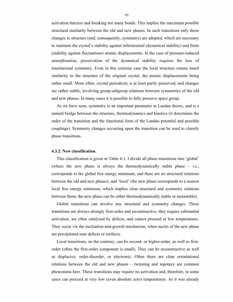
95
activation barriers and breaking too many bonds. This implies the maximum possible
structural similarity between the old and new phases. In such transitions only those
changes in structure (and, consequently, symmetry) are adopted, which are necessary
to maintain the crystal’s stability against infinitesimal (dynamical stability) and finite
(stability against fluctuations) atomic displacements. In the case of pressure-induced
amorphisation, preservation of the dynamical stability requires the loss of
translational symmetry. Even in this extreme case the local structure retains much
similarity to the structure of the original crystal, the atomic displacements being
rather small. More often, crystal periodicity is at least partly preserved, and changes
are rather subtle, involving group-subgroup relations between symmetries of the old
and new phases. In many cases it is possible to fully preserve space group.
As we have seen, symmetry is an important parameter in Landau theory, and is a
natural bridge between the structure, thermodynamics and kinetics (it determines the
order of the transition and the functional form of the Landau potential and possible
couplings). Symmetry changes occurring upon the transition can be used to classify
phase transitions.
4.3.2. New classification.
This classification is given in Table 4-1. I divide all phase transitions into ‘global’
(where the new phase is always the thermodynamically stable phase – i.e.,
corresponds to the global free energy minimum, and there are no structural relations
between the old and new phases), and ‘local’ (the new phase corresponds to a nearest
local free energy minimum, which implies clear structural and symmetry relations
between them; the new phase can be either thermodynamically stable or metastable).
Global transitions can involve any structural and symmetry changes. These
transitions are always strongly first-order and reconstructive, they require substantial
activation, are often catalysed by defects, and cannot proceed at low temperatures.
They occur via the nucleation-and-growth mechanism, when nuclei of the new phase
are precipitated near defects or surfaces.
Local transitions, on the contrary, can be second- or higher-order, as well as first-
order (often the first-order component is small). They can be reconstructive as well
as displacive, order-disorder, or electronic. Often there are clear orientational
relations between the old and new phases – twinning and topotaxy are common
phenomena here. These transitions may require no activation and, therefore, in some
cases can proceed at very low (even absolute zero) temperatures. As it was already
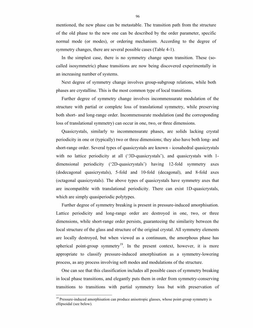
96
mentioned, the new phase can be metastable. The transition path from the structure
of the old phase to the new one can be described by the order parameter, specific
normal mode (or modes), or ordering mechanism. According to the degree of
symmetry changes, there are several possible cases (Table 4-1).
In the simplest case, there is no symmetry change upon transition. These (so-
called isosymmetric) phase transitions are now being discovered experimentally in
an increasing number of systems.
Next degree of symmetry change involves group-subgroup relations, while both
phases are crystalline. This is the most common type of local transitions.
Further degree of symmetry change involves incommensurate modulation of the
structure with partial or complete loss of translational symmetry, while preserving
both short- and long-range order. Incommensurate modulation (and the corresponding
loss of translational symmetry) can occur in one, two, or three dimensions.
Quasicrystals, similarly to incommensurate phases, are solids lacking crystal
periodicity in one or (typically) two or three dimensions; they also have both long- and
short-range order. Several types of quasicrystals are known - icosahedral quasicrystals
with no lattice periodicity at all (‘3D-quasicrystals’), and quasicrystals with 1-
dimensional periodicity (‘2D-quasicrystals’) having 12-fold symmetry axes
(dodecagonal quasicrystals), 5-fold and 10-fold (decagonal), and 8-fold axes
(octagonal quasicrystals). The above types of quasicrystals have symmetry axes that
are incompatible with translational periodicity. There can exist 1D-quasicrystals,
which are simply quasiperiodic polytypes.
Further degree of symmetry breaking is present in pressure-induced amorphisation.
Lattice periodicity and long-range order are destroyed in one, two, or three
dimensions, while short-range order persists, guaranteeing the similarity between the
local structure of the glass and structure of the original crystal. All symmetry elements
are locally destroyed, but when viewed as a continuum, the amorphous phase has
spherical point-group symmetry19. In the present context, however, it is more
appropriate to classify pressure-induced amorphisation as a symmetry-lowering
process, as any process involving soft modes and modulations of the structure.
One can see that this classification includes all possible cases of symmetry breaking
in local phase transitions, and elegantly puts them in order from symmetry-conserving
transitions to transitions with partial symmetry loss but with preservation of 19 Pressure-induced amorphisation can produce anisotropic glasses, whose point-group symmetry is ellipsoidal (see below).
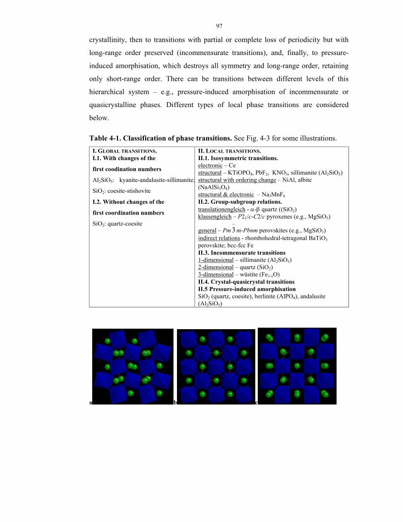
97
crystallinity, then to transitions with partial or complete loss of periodicity but with
long-range order preserved (incommensurate transitions), and, finally, to pressure-
induced amorphisation, which destroys all symmetry and long-range order, retaining
only short-range order. There can be transitions between different levels of this
hierarchical system – e.g., pressure-induced amorphisation of incommensurate or
quasicrystalline phases. Different types of local phase transitions are considered
below.
Table 4-1. Classification of phase transitions. See Fig. 4-3 for some illustrations.
I. GLOBAL TRANSITIONS. I.1. With changes of the
first coodination numbers
Al2SiO5: kyanite-andalusite-sillimanite;
SiO2: coesite-stishovite
I.2. Without changes of the
first coordination numbers
SiO2: quartz-coesite
II. LOCAL TRANSITIONS. II.1. Isosymmetric transitions. electronic – Ce structural – KTiOPO4, PbF2, KNO3, sillimanite (Al2SiO5) structural with ordering change – NiAl, albite (NaAlSi3O8) structural & electronic – Na3MnF6 II.2. Group-subgroup relations. translationengleich - α-β quartz ((SiO2) klassengleich – P21/c-C2/c pyroxenes (e.g., MgSiO3)
general – Pm−3 m-Pbnm perovskites (e.g., MgSiO3)
indirect relations - rhombohedral-tetragonal BaTiO3 perovskite; bcc-fcc Fe II.3. Incommensurate transitions 1-dimensional – sillimanite (Al2SiO5) 2-dimensional – quartz (SiO2) 3-dimensional – wüstite (Fe1-xO) II.4. Crystal-quasicrystal transitions II.5 Pressure-induced amorphisation SiO2 (quartz, coesite), berlinite (AlPO4), andalusite (Al2SiO5)
a b c

98
d e f
g h i
j k Fig. 4-3. Examples of different phase transitions. (a-c) different perovskite phases (a-
Pbnm, b-I4/mcm, c- Pm−
3 m). Green spheres – Mg atoms. (d-f) Al2SiO5 polymorphs (d-kyanite, e-andalusite, f-sillimanite). Al polyhedra are shown in yellow and turquoise. (g-k) silica polymorphs (g- α-quartz, h – β-quartz, i- coesite, j- stishovite, k- CaCl2-type structure, drawn with an exaggerated orthorhombic distortion). Si-polyhedra are shown in blue.
4.3.3. Phenomenology and examples of local phase transitions.
4.3.3.1. Isosymmetric transitions.
Using Landau theory, it is easy to show that isosymmetric transitions must be
first-order, but can disappear (i.e. become fully continuous, infinite-order transitions)
at the critical point and above it (Bruce & Cowley, 1981; Christy, 1995). There is a
complete analogy here with the liquid-gas transitions (which are also isosymmetric).
At supercritical temperatures there are generally rapid, but continuous changes in all
properties along any p-T path going above the critical point (Angel, 1996). Second-
order phase transitions must involve changes in space group symmetry. All examples
known so far fully confirm these theoretical conclusions.
99
Another example of isosymmetric phase transition phenomena outside the realm
of solids is given by the newly discovered liquid-liquid phase transitions (McMillan,
2000), which are also first order with a critical point terminating the two-phase
equilibrium line. Phase transition between structurally different amorphous phases20
of ice was observed (Mishima et al., 1985) and reported to be first order.
Increasingly many crystals are now known to exhibit crystal-crystal isosymmetric
phase transitions (i.e. those for which both phases have the same space group with
the same number of atoms in the unit cell, with atoms occupying the same Wyckoff
positions). Such transitions can be electronic (where the electronic structure changes
– e.g., Ce and SmS), structural (where coordination numbers of atoms change
discontinuously – e.g., KTiOPO4) or intermediate (both electronic and structural
changes are involved – e.g., Na3MnF6). Another kind of structural isosymmetric
transitions associated to the change of the ordering of atoms or defects was recently
predicted for the Al-rich NiAl alloy (Alavi et al., 1999) and albite NaAlSi3O8
(Oganov et al., 2001c).
Electronic transitions. Metallic Ce undergoes an isosymmetric phase transition
Ce(I)-Ce(IV) (see Liu & Bassett, 1986, and references therein), presumably due to
6s-4f (or 5d) electronic transition. Both Ce(I) and Ce(IV) have the fcc structure
(space group Fm−
3 m). The volume change at the transtion is very large (13%) at
room temperature, but it rapidly decreases along the Ce(I)-Ce(IV) equilibrium line
until it disappears at the critical point (2.15 GPa and 613 K). Corundum-type Co2O3
(space group R−
3 c) undergoes an isosymmetric phase transformation, accompanied
by a significant volume reduction (6.4 % at zero pressure), at ~8 GPa and 1123 K
(see Liu & Bassett, 1986, and references therein). This transition does not alter the
structure type and is thought to be due to the high-spin - low-spin electronic
transition. Another famous example of an electronic transition is SmS, which
transforms from the low-pressure insulating phase to the high-pressure metallic
phase; both phases have a NaCl-type structure. Fig. 4-4 explains this transition.
20 All liquid, gaseous, and conventional amorphous phases are isosymmetric, having spherical point-group symmetry.
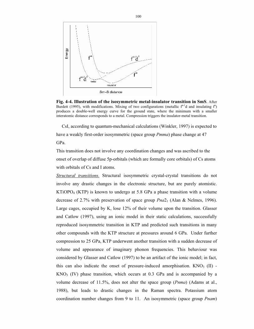
100
Fig. 4-4. Illustration of the isosymmetric metal-insulator transition in SmS. After Burdett (1995), with modifications. Mixing of two configurations (metallic fn-1d and insulating fn) produces a double-well energy curve for the ground state, where the minimum with a smaller interatomic distance corresponds to a metal. Compression triggers the insulator-metal transition.
CsI, according to quantum-mechanical calculations (Winkler, 1997) is expected to
have a weakly first-order isosymmetric (space group Pmma) phase change at 47
GPa.
This transition does not involve any coordination changes and was ascribed to the
onset of overlap of diffuse 5p-orbitals (which are formally core orbitals) of Cs atoms
with orbitals of Cs and I atoms.
Structural transitions. Structural isosymmetric crystal-crystal transitions do not
involve any drastic changes in the electronic structure, but are purely atomistic.
KTiOPO4 (KTP) is known to undergo at 5.8 GPa a phase transition with a volume
decrease of 2.7% with preservation of space group Pna21 (Alan & Nelmes, 1996).
Large cages, occupied by K, lose 12% of their volume upon the transition. Glasser
and Catlow (1997), using an ionic model in their static calculations, successfully
reproduced isosymmetric transition in KTP and predicted such transitions in many
other compounds with the KTP structure at pressures around 6 GPa. Under further
compression to 25 GPa, KTP underwent another transition with a sudden decrease of
volume and appearance of imaginary phonon frequencies. This behaviour was
considered by Glasser and Catlow (1997) to be an artifact of the ionic model; in fact,
this can also indicate the onset of pressure-induced amorphisation. KNO3 (II) -
KNO3 (IV) phase transition, which occurs at 0.3 GPa and is accompanied by a
volume decrease of 11.5%, does not alter the space group (Pnma) (Adams at al.,
1988), but leads to drastic changes in the Raman spectra. Potassium atom
coordination number changes from 9 to 11. An isosymmetric (space group Pnam)
101
phase change has been observed at 9.8 GPa for PbF2 (Haines et al., 1998). The
volume difference between the phases was estimated to be 2-3% at 1 atm. X-ray
diffraction structure refinement has shown that structural topology undergoes only
minor changes, and Pb atom coordination changes from 9 to 10. Compression
experiments (Hugh-Jones & Angel, 1994) suggest that orthoenstatite (MgSiO3) may
have a weakly first-order (∆V/V=0.09%, of the order of experimental uncertainties)
isosymmetric transition at 4 GPa. At this pressure sudden changes in the mechanism
of compression were observed. Another possible case for isosymmetric
polymorphism is anorthite CaAl2Si2O8, where an isosymmetric I−
1 - I−
1
transformation was postulated in order to account for the unusually high curvature of
the P−
1 - I−
1 equlibrium line on the phase diagram (Angel, 1996). X-ray structure
determinations seem to support this hypothesis, showing significant differences in
high-presure and high-temperature structures of the I−
1-phase, and very rapid
structural changes of this phase at changing p and T are probably associated with
crossover above the critical point. In their molecular dynamics simulations, Badro et
al. (1996) found that quartz (SiO2) irreversibly amorphised under hydrostatic
pressure of 22 GPa, but transformed into a crystalline phase with all silicon atoms in
a 5-fold coordination when subjected to a uniaxial stress (20 GPa along the a and b
axes and 27 GPa along the c direction). Later, Badro et al. (1997) commented that
this phase is isosymmetric with quartz (space group P3221). It was reproduced in ab
initio LDA simulations; semiclassical simulations demonstrated its dynamical
stability. On decompression, this phase reverted to quartz through an intermediate
phase with strongly distorted SiO4-tetrahedra, and on increasing the uniaxial stress it
amorphised. The amorphous phase was structurally different from the pressure-
amorphised quartz, and on decompression transformed into a defective quartz-like
material at 10 GPa.
Na3MnF6 (space group P21/n) is an example of a phase transition with a
simultaneous change in the atomic and electronic structure. At 2.2 GPa this
compound undergoes a first-order isosymmetric phase transformation, which is
associated with a change of orientation of the Jahn-Teller elongation of MnF6
octahedra (Carlson et al., 1998). The transformation shows a small hysteresis of 0.5
GPa.

102
Anticipation of isosymmetric phase transitions, associated with a change of atomic
or defect ordering. Alavi et al. (1999) have demonstrated the possibility of pressure-
induced isosymmetric phase transitions in non-stoichiometric systems with different
possible ways of defect ordering. They studied the non-stoichiometric alloy Ni1-
xAl1+y with excess of Al relative to Ni related either to the Ni vacancies or to the Al
atoms occupying some of the Ni sites (‘antisite’ structure). The first structure has
lower density and energy and at high pressures becomes less stable than the antisite
structure. Using ab initio calculations, Alavi et al. (1999) have predicted the phase
diagram of this alloy with a first-order isosymmetric phase transition between the
defect structures, critical point behaviour, and coexistence of both defect
configurations in the alloy above the critical point. My semiclassical calculations
(Oganov et al. 2001c; Chapter 6) predict that triclinic (P−
1) Na-feldspar, albite
NaAlSi3O8, undergoes an isosymmetric phase transition associated with a change of
the Al-Si ordering scheme, induced by non-hydrostatic stresses or high pressure. At
low pressures the Al atoms predominantly occupy the T1 tetrahedral sites, while at
high pressures Al prefers the T2 tetrahedral sites.
103
4.4.3.2. Transitions with group-subgroup relations.
There are several possibilities here, springing from different types of
subgroups/supergroups of crystal symmetry. According to Hermann theorem (Hahn
& Wondratshcek, 1994), a maximal subgroup of a space group is either
Translationengleich21-type (i.e., all translations are preserved, but some of the point-
group symmetry operators disappear) or Klassengleich22-type (all point-group
operators are preserved, but some of the lattice translations disappear; as a
consequence, a superstructure is formed). Subgroups, which are neither
klassengleich, nor translationengleich, are called general subgroups; they involve
both cell multiplication and lowering of the point-group symmetry. Examples are
α→β quartz (translationengleich), P21/c-C2/c pyroxenes (klassengleich; see very
interesting papers by Arlt & Angel, 2000 and Arlt et al., 1998), and Pbnm→Pm−
3 m
transitions in perovskites (general).
The fourth type of transitions with group-subgroup transitions involves indirect
symmetry relations between two phases via an intermediate archetypal phase of a
higher symmetry, which is a supergroup for symmetries of both phases. An example
is BaTiO3, where the transition between the rhombohedral and tetragonal phases can
be described with reference to the higher-symmetry cubic phase. Such transitions are
usually weakly first-order.
Yet another possibility is that of a transition state of a lower symmetry, which is a
common subgroup of the symmetries of both phases. These transitions are usually
strongly first-order; often they can be described as reconstructive (see Christy,
1993). The fcc→bcc transition in Fe can be described with reference to lower-
symmetry tetragonal or rhombohedral configurations, whose symmetries are
common subgroups of both symmetry groups of the bcc and fcc phases. Recent
works of H. Sowa were dedicated to finding transition paths between simple
elementary and binary structure types on the basis of symmetry. E.g., Sowa (2000
and personal communication) concluded that the transition from the sphalerite (ZnS)
to the NaCl-type is most likely to proceed via an orthorhombic transition state. Catti
(2001) performed accurate ab initio calculations for SiC and arrived at the same
21 German word meaning ‘having the same translations’; accepted as an international term (International Tables for Crystallography) 22 German word meaning ‘having the same (point-group) class’; accepted as an international term (International Tables for Crystallography)
104
conclusion, in conflict with the traditionally accepted rhombohedral transition state
for this material.
4.4.3.3. Incommensurate transitions.
Incommensurate transitions are a topic of enormous current research. I shall not
discuss these phases in detail, but refer the reader to a review (van Smaalen, 1995)
and some interesting papers – on theory of incommensurate transitions in insulators
(Heine & McConnell, 1981) and on unusual crystal morphology of incommensurate
phases (Dam et al., 1985). Incommensurability can occur via mode softening or
modulation of atomic positional occupancies, or in metals via electronic effects (e.g.,
Peierls transition). These are typical local transitions. They occur in a large number
of compounds (e.g., NaNO2) and minerals (some intermediate plagioclase feldspars,
nepheline (K,Na)AlSiO4, akermanite Ca2MgSi2O7, calaverite AuTe2, wüstite Fe1-xO;
there is an incommensurate phase in quartz, intermediate between α- and β-phases).
Incommensurate modulation can occur in 1, 2, or 3 dimensions. An incommensurate
phase is predicted for sillimanite in Chapter 9 (Oganov et al., 2001d).
4.4.3.4. Crystal-quasicrystal transitions.
The first quasicrystal (Al86Mn14) was discovered relatively recently (Shechtman et
al., 1984). Now we know a large number of quasicrystals, theories of their structure
and formation have been formulated, and even some computational studies
performed. For a review, see Janot (1994). Quasicrystals have both short- and long-
range order, but lack translational periodicity in one or (usually) more dimensions.
They can have symmetry axes incompatible with translational periodicity – 5-fold
axed in icosahedral quasicrystals, 5- and 10-fold axes in decagonal, 8-fold axes in
octagonal, and 12-fold axes in dodecagonal quasicrystals. These 2– and 3-
dimensional quasicrystals are described by 2- or 3-dimensional Penrose tilings (Fig.
4-5) with two or more types of ‘unit cells’. All quasicrystals are metallic alloys, most
are metastable, but some are thermodynamically stable.

105
Fig. 4-5. Penrose tiling for a decagonal quasicrystal. White and black tiles are different ‘unit cells’ having different compositions. The ratio of white tiles to the black ones is the golden mean τ=( 5 +1)/2.
Although not known definitively, it is likely that crystal-quasicrystal transitions
are local. However, an ideal crystal and ideal quasicrystal are not very likely
(although can in principle) to have the same composition. Since the proportion of
different tiles, or ‘unit cells’, in a Penrose tiling is irrational, general quasicrystal
composition will be characterised by a chemical formula with irrational coefficients
(see Janot, 1994). This explains both the extremely complicated chemical formulae
of quasicrystals, and their occurrence exclusively among metallic alloys, where
charge balance considerations are not applicable (an ionic or covalent solid cannot
have an irrational chemical formula as this would break charge neutrality). Ideal
stoichiometric crystals, on the other hand, must have a rational chemical formula, in
accord with Dalton’s law. Therefore, crystal-quasicrystal transitions are most likely
to occur between disordered and non-stoichiometric states. Terminological curiosity:
quasicrystals, which can be daltonides23, do not obey Dalton’s law.
23 i.e. materials which have a constant composition, as opposed to bertollides, which are defined as non-stoichiometric compounds.

106
4.4.3.5. Pressure-induced amorphisation.
This phenomenon was first discovered in 1984 in experiments on compression of
ice (Mishima et al., 1984), which, compressed to 1 GPa at 77 K, did not transform to
the modification stable at these conditions (ice VI), but was found to amorphise.
Since 1984, large efforts were made to understand the physics of this unusual type of
phase transformations, but many questions remain open. Here I give only a brief
overview; for detailed reviews see excellent papers (Sharma & Sikka, 1996; Richet
& Gillet, 1997).
A great number of crystals undergoing pressure-induced amorphisation is
known24, as well as a few substances undergoing an opposite phenomenon –
pressure-release amorphisation (for extensive reviews, see Sharma & Sikka, 1996;
Richet & Gillet, 1997). In the latter phenomenon, high-pressure phases, when
decompressed to pressures well below their stability fields, become dynamically
unstable and amorphise25.
Pressure-induced amorphisation is always a metastable first order transition. It
requires that the amorphous phase be denser than the original crystalline phase. This
means that crystals with open structures should be easier to amorphise in contrast to
close packed ones.
Structural relationships between melting-and-cooling-produced amorphous phases
and pressure-induced ones are still widely discussed. A similar, also widely
discussed, question is about the degree of similarity of the processes of melting and
amorphisation under pressure. It is often stated that pressure-induced amorphisation
occurs on the metastable extension of the melting curve, in cases where the melting
temperature decreases with pressure. This idea has received experimental support for
several systems (see Richet & Gillet, 1997; Mishima, 1996; Hemley et al., 1988), but
its generality is questionable, because melts and pressure-amorphised glasses can be
structurally very different. For ice, the two amorphous phases (one produced by
cooling water, the other - by pressurising ice) are separated by a first-order phase
transition (Mishima et al., 1985), which indicates clear structural differences.
Pressure-induced amorphisation occurs in the limit of dynamical stability of the
crystal. In melting, the temperature of the onset of a mechanical instability gives an 24 Quartz SiO2, coesite SiO2, berlinite AlPO4, GeO2, zeolites scolecite Ca8Al16Si24O80*24H2O and mesolite Na16Ca16Al48Si72O240*64H2O, anorthite CaAl2Si2O8, forsterite Mg2SiO4, fayalite Fe2SiO4, wollastonite CaSiO3, enstatite MgSiO3, muscovite KAl3Si3O10(OH)2, serpentine Mg3Si2O5(OH)4, portlandite Ca(OH)2 are just a few examples.
107
upper bound of the true thermodynamic melting temperature: solids cannot be
overheated to higher temperatures. This temperature can be used as a first
approximation to the true melting temperature (e.g., MD simulations of Vočadlo &
Price, 1996; Chaplot et al., 1998, and comment by Belonoshko, 2001).
Behaviour of pressure-induced amorphous phases on decompression can be very
different: some compounds (e.g., Ca(OH)2) recrystallise into a fine-grained
aggregates, others (e.g., SiO2, ice) remain amorphous. Berlinite (AlPO4) is known for
exhibiting the so called “memory glass effect”: the amorphous phase, appearing
under compression of a single crystal of berlinite under 18 GPa, on decompression to
5 GPa turns back to the single crystal with the same crystallographic orientation
(Kruger & Jeanloz, 1990). Brillouin spectroscopy (Polian et al., 1993) confirmed this
effect, with a hysteresis loop between 7 and 15 GPa. The amorphous phase turned
out to be elastically anisotropic. MD calculatons (Tse & Klug, 1992) successfully
reproduced the memory glass effect, with considerable short-range order and long-
range disorder. Gillet et al. (1995) suggested that the ‘memory glass effect’ was an
experimental artifact. According to these authors, berlinite transformed into an
intermediate strongly disordered crystalline phase at 15 GPa, and the true
amorphisation occurred at higher pressures and was irreversible26.
Elastic anisotropy was also found in pressure-amorphised quartz by Brillouin
spectroscopy (McNeil & Grimsditch, 1991) and MD simulations (Tse & Klug,
1993). The latter study found no structural relationships between pressure-
amorphised quartz and silica glass.
Mechanisms driving pressure-induced amorphisation are still not quite clear. The
necessary conditions are: 1) Higher density of the amorphous phase compared to the
crystalline one. Usually it means that coordinaton numbers increase on
amorphisation; 2) Presence of soft modes in the crystalline phase. Softening of a
vibrational mode at a single point of the Brillouin zone should drive a transition to a
crystalline (if the soft wavevector is rational) or incommensurate (if the wavevector
is irrational) phase. Only simultaneous or nearly simultaneous softening of a phonon
branch at a range of k-vectors (e.g., along a special direction of the Brillouin zone)
can produce an amorphous phase (Keskar et al., 1994; Binggeli et al., 1994;
Hemmati et al., 1996). Any atomic displacement, expressible as a combination of 25 This happens to the perovskite-structured modification of CaSiO3, one of the main minerals of the Earth’s lower mantle, which at ambient conditions turns to a glass within a few hours.

108
soft modes, lowers the energy; the multitude of possible combinations gives rise to
the disorder. However, a large degree of order should remain: because the
displacements are expected to be small and because only displacements related to the
softening phonon branch are allowed to freeze in. Simultaneous softening of a
phonon branch along a direction in the Brillouin zone implies weak dispersion of this
branch, which is most naturally achieved when the unit cell is large. Indeed, crystals
with complicated structures and large unit cells are more prone to pressure-induced
amorphisation.
4.4. Discussion of the new classification.
The classification presented above is based on symmetry and naturally
incorporates the old notions of first-order and continuous, reconstructive, displacive,
order-disorder, and electronic phase transitions. Its principles are very simple, but
like any classification it is not perfect. The weak point is in the distinction between
local and global transitions. Such a distinction is rigorously made only by
considering the free energy hypersurfaces, but in practice we make it by saying that
the structures are ‘related’ or ‘unrelated’.
Continuous paths (i.e. some structural relation) can in principle be constructed
between any two structures, however different27. However, for strongly
reconstructive (global) transitions none of these paths will be followed because of
the high energy barriers required. A useful criterion of locality of a transition is given
by the comparison of the shapes and parameters of the supercells and looking at the
structures along possible transition paths. Yet, the transition between andalusite and
sillimanite (Al2SiO5), here considered as global, would emerge close to local
transitions. On the other hand, some transitions considered as local (especially
among the indirect group-subgroup transitions) involve large atomic displacements.
Examples are given by polytypic and order-disorder transformations, both of which
are kinetically hindered at low temperatures.
Forces in crystals obey the space group symmetry, and will tend to preserve it.
Most phase transitions, however, change crystal symmetry, usually by a group-
subgroup scheme. Isosymmetric transitions remain a rare, but fundamentally
important phenomenon. The present classification emphasises the fundamental role 26 This seems to be a general conclusion. However, memory glass effect has also been reported for other systems, e.g. the equimolar solid solution Ca(NO3)2:NaNO3 (Winters et al., 1992).
109
of isosymmetric polymorphism and pressure-induced amorphisation as the two
extreme cases of symmetry changes.
Ostwald rule can now be formulated in new terms: ‘Global phase transformations
tend to occur via a sequence of local metastable transitions’. Theoretically, for any
compound there can be an infinite number of metastable structures, corresponding to
local minima of the free energy hypersurface. However, only a handful of these
possibilities can practically be synthesised. One expects that phases, most likely to
appear as metastable in synthesis, must either be stable at some p-T conditions, or be
related to one of the stable phases by a local phase transition. In other words, there
must be structural and symmetry relation between the possible metastable phases and
the stable phases. Locality, as a major principle governing the selection of possible
metastable phases, should be important for planned synthesis of technologically
important metastable compounds.
27 The simplest way to do this is to consider for both structures supercells with the same number of atoms. An infinite number of continuous transition paths between these supercells can be constructed.
110
Chapter 5. Simulation methods.
In this chapter I shall give an account of some of the most important advances of
modern theoretical physics and their use in state-of-the-art computer simulation of
condensed matter. At times this account will be only glancing; for more details there
exist a number of excellent reviews and original papers. General references include
several books (Born & Huang, 1954; Urusov, 1975; Catlow & Mackrodt, 1982;
Allen & Tildesley, 1987; Urusov & Dubrovisky, 1989; Tossell & Vaughan, 1992;
Dove, 1993; Sutton, 1993; Thijssen, 1999) and review articles (Catti, 1986; Catlow
& Price, 1990; Catlow et al., 1993, 1994; Gavezzotti, 1994; Bukowinski, 1994;
Cohen, 1994, 1999; Hemley & Cohen, 1996; Gale, 1996; Stixrude et al., 1998; Kohn,
1999a,b). Computer simulations represent one of the fastest-growing areas of
physics, and new methods and significant developments appear continually.
First I consider the current state and predictive power of theoretical crystal
chemistry. The I proceed with formulating the general quantum-mechanical problem
and the Born-Oppenheimer principle, which will be followed by a discussion of
quantum-mechanical methods. Both advances and problems of state-of-the-art
quantum-mechanical computational methods will be discussed, as well as future
areas of their development. Then, I discuss interatomic interactions and their
analytical representation, with the advantages and deficiencies of this approach. The
chapter finishes with a description of dynamical simulations via lattice dynamics and
molecular dynamics methods.
5.1. An essay on the state of the art of predictive crystal chemistry.
The main task of any theoretical science is the explanation of known and the
prediction of unknown facts. For crystal chemistry this is the task of predicting
structure, properties, and stability fields of all possible modifications for a given
compound. The last 20 years have seen an enormous progress towards this goal, yet
we are still far from it. Nearly all modern methods start with a given topology of the
crystal structure, which is then refined to the theoretically optimal structure.
Knowing just the structural topology, for most compounds it is possible to accurately
predict many properties and behaviour at high temperatures/pressure (Catlow &
Mackrodt, 1982; Catti, 1986; Urusov & Dubrovinsky, 1989; Сatlow & Price, 1990;
Burnham, 1990; Silvi, 1991; Dovesi et al., 1992; Catlow et al., 1993; Catlow et al.,
111
1994; Bukowinski, 1994); if there are several candidate phases with known
topologies, it is possible to construct a theoretical phase diagram. Prediction of the
topology itself (i.e., the structure type) is possible in some cases (Burdett, 1988;
Urusov et al., 1990), but successes here are rather modest.
5.1.1. Modern theoretical and predictive crystal chemistry.
Concepts and rules of crystal chemistry, largely empirical, allow one to obtain the
simplest qualitative and semiquantitative predictions for the structure of materials.
They are also essential for the understanding of crystal structures, their stability, and
properties. The most important ones include the concept of atomic and orbital
electronegativities (e.g., Pauling, 1960; Urusov, 1975; 1987; Allen, 1989; Baekelandt
et al., 1991), Pauling’s rules for ionic and covalent crystals (Pauling, 1960), systems
of atomic and ionic radii (see Urusov, 1987), concept of close packing (Belov, 1947);
the notion of the valence electron concentration for metals and alloys (e.g., Urusov,
1987); for covalent crystals – Grimm-Sommerfeld and Hume-Rothery rules, and
Parthé rules (Parthé, 1996; Urusov, 1987). Burdett and McLarnan (1984) showed
why Pauling’s rules work and, furthermore, why they are applicable not only to ionic
crystals (as originally formulated by Pauling), but also to crystals with a significant
covalent component of bonding (e.g., silicates). Brown’s extension of the second
Pauling’s rule (Brown, 1992) appears to be applicable to all chemical systems. A
justification of this universality was given by Urusov (1995). Topological analysis of
the electron density due to Bader (Bader, 1990) also justifies Brown’s rule (see, e.g.,
Tsirelson, 1993). The topological analysis itself is a significant advance in theory – it
defines a scheme of partitioning of the space into atomic regions, justifies the
additivity of atomic properties, and allows one to define atomic charges, volumes,
etc.
An example of an old elegant idea, evolving until today, is the VSEPR (Valence
Shell Electron Pair Repulsion) model. Pseudopotential radii (Zunger, 1980) brought
a new systematics of atomic properties relevant to chemical bonding, being
simultaneously a measure of the atomic size (e.g., atomic radii – Ganguly, 1993) and
an inverse measure of the electronegativity (Zunger, 1980). It was shown that at least
for binary systems each structure type occupies a separate domain on the 2D-map
whose axes are linear combinations of the orbital pseudopotential radii of the atoms.
Each chemical composition falls in one of these domains, giving the most likely
structure. These predictions are remarkably successful at least for binary compounds

112
(Zunger, 1980; Burdett, 1988; Ych at al., 1992). Compositions likely to produce
quasicrystals were predicted using this method as well (Villars et al., 1986).
Since the 1960-s it has become possible to study both experimentally and
theoretically electron density distribution in crystals (Coppens, 1992, 1997;
Tsirelson, 1993; Tsirelson et al., 1986), accurate thermal motion parameters
(Tsirelson, 1993), and study crystals at the temperatures and pressures of the Earth’s
interior. One of the greatest advances in theory was the ability to extend quantum-
mechanical calculations to crystals, and to perform such calculations at arbitrary
temperatures and pressures for relatively large systems (routinely up to ~100 atoms;
in some studies up to ~30,000 atoms!). Less expensive (by ~103 times), but more
restricted in accuracy, semiclassical simulations based on analytical representations
of interatomic interactions can be used to study very large systems (up to millions of
atoms). The semiclassical approach, due to its low computational cost, is suitable for
systematic searches of possible structure types for a given compound. Such studies,
based on either genetic algorithms (Bush et al., 1995; Gallagher et al., 1991), or
simulated annealing (Pannetier et al., 1990), or other methods, show a great promise.
In the rest of this chapter, I will describe the foundations and some technical
details of both quantum-mechanical and semiclassical simulations. First, I will
outline the general problem, then describe methods for calculating the internal
energy (static calculations), and then describe dynamical simulations.
5.2. Formulation of the general problem and the Born-Oppenheimer principle.
In the thermodynamic limit, any system attains the state with the lowest Gibbs
free energy G at given p-T conditions:
G(p,T)→min (5.2.1)
All equilibrium structural and electronic parameters can be determined by
minimising G = E + pV - TS. Many ground-state properties can then be obtained by
differentiating G, e.g. with respect to the structural parameters. This general task is
very difficult, and is solved in several steps, by making several consequtive
approximations.
The first step is to decouple the electronic and structural (nuclear) degrees of
freedom. In all practical calculations (and in experimental studies of structure and
electron density) the adiabatic Born-Oppenheimer principle is assumed to hold. This
principle states that, since masses of atomic nuclei are much (thousands of times)
113
larger than masses of electrons, atomic motion will be much slower than electronic.
As a consequence, electrons will almost instantaneously relax to the ground state
every time an atom displaces. This allows one to decouple the electronic and atomic
degrees of freedom, and consider the quantum-mechanical problem in the framework
of fixed nuclei, whose positions determine the ground-state electronic wavefunction.
This is an approximation: in reality it will always take some finite time for the
electrons to adjust to changing nuclear positions; however, this approximation is
extremely accurate (it may possibly break down only for the lightest elements). It
allows one to define the (adiabatic) energy hypersurface in terms of only atomic
degrees of freedom: each structural configuration has a unique and definite value of
the energy. Problems with the adiabatic principle occur when there are two or more
electronic states which have the same symmetry and are very close in energy for a
given structural configuration: this would result in mixing of the ground and excited
states. For metals and semiconductors at finite temperatures, the excited states will
be partly occupied according to the Fermi-Dirac statistics, giving some electronic
contribution to the entropy and free energy. In insulators, this contribution will be
negligible up to very high temperatures (well above 10,000 K).
The next step in solving this problem is to define the internal energy hypersurface.
At each configuration, the internal energy can be calculated either by solving the
electronic Schrödinger equation, or by using semiclassical parameterised models of
interatomic interactions. Minimising the internal energy E is equivalent to the free
energy minimisation at p=0 and T=0 K. Knowing the internal energy hypersurface,
we can always calculate the entropy S and minimise the free energy G. Ideally, one
would solve the nuclear Schrödinger equation and find all energy levels in the
system, with which one can next calculate the partition function, eq. (3.1.1), and all
the thermodynamic properties including the free energy, eq. (3.1.2)). Solving the
Schrödinger equation for an arbitrary multi-dimensional energy hypersurface is
exceedingly difficult, and two common ways of solving this problem are: 1) to use
the classical approximation for nuclear motion (as in molecular dynamics and Monte
Carlo simulations; this approach is valid at high temperatures) and 2) to solve the
Schrödinger equation assuming that the system is harmonic (this approach is used in
lattice dynamics simulations and is valid at relatively low temperatures). First, I will
discuss the methods of calculating the energy, and then describe lattice dynamics and
molecular dynamics simulations, which take temperature into account.
114
5.3. Methods of calculating the internal energy.
The total energy of an electron-nuclear system and all its energy levels can be
calculated by solving the Schrödinger equation: ∧
H ψ = Eψ (5.3.1)
where ∧
H is the Hamiltonian operator of the system. Here I consider only the non-
relativistic theory, sufficient when atoms lighter than krypton are treated28. Writing ∧
H more explicitly, in atomic units29 we have:
[∑=
N
i 1( -1/2 2
i∇ ) + ∑=
N
iiv
1n-e )(r + ∑
= −
N
i ji1 ||1
rr]ψ = Eψ , (5.3.2)
where N is the number of electrons. The first term in (5.3.2) is the kinetic energy
operator and the following terms are the electron-nuclear and electron-electron
potential energy operators, respectively; E is the electronic energy (to find the total
energy, one needs to add to it the nuclear-nuclear interaction energy). Schematically,
we can write (5.3.2) as follows:
(-1/2∇ 2 + ve-n + ve-e)ψ = Eψ (5.3.3)
28 Relativistic effects appear when electrons are moving at speeds comparable to the speed of light.
This situation occurs only in heavy atoms, where the inner electrons move in a very strong nuclear
potential. Two main manifestations of relativity in the electronic structure are scalar relativistic effects
(shrinking of the innermost atomic orbitals, which also affects the potential acting on the valence
electrons) and spin-orbit interaction. To see how scalar relativistic effects occur (Pisani, 1996), note
that the average velocity of a 1s electron in atomic units is Z (nuclear charge), and the speed of light is
137.036 a.u. For Hg (Z=80) the relativistic mass of a 1s electron is 1.23 times its rest mass. This
corresponds to a ~23% shrinking of the 1s-orbital in Hg, since the Bohr radius (a0=22 / meh ) is
inversely proportional to the mass of the electron. Shrunk core orbitals more effectively screen the
outer orbitals; due to orthogonality with the innermost electrons, valence s- and p-electrons become
contracted and stabilised relative to the non-relativistic case, whereas valence d- and f-electrons
become more expanded, destabilised, and thus more chemically active. Spin-orbit interaction becomes
important in heavier atoms (roughly after Xe); in solids it can remove degeneracies of electron levels
at high-symmetry points of the reciprocal space (Aschcroft & Mermin, 1976). Spin-orbit interaction
adds a term, proportional to the dot-product of the electron spin moment and the vector product of its
velocity and the electric field, to the potential acting on the electron. For a fully relativistic treatment,
one must solve the Dirac (rather than Schrödinger) equation. For a detailed review of relativistic
effects in chemistry and the existing relativistic computational methods, see Pyykko (1988). 29 In atomic units, ħ = me = e2 = 4πε0 = 1. The units of length and energy in this system are Bohr
radius a0=0.529 Å and Hartree (equal to minus twice the energy of the hydrogen atom): 1 Ha=27.2116
eV. Atomic units are used in all quantum-mechanical equations in this chapter.

115
The Hamiltonian is in principle very simple, having only Coulombic interactions.
The main problem in solving (5.3.2) is that the wavefunction is a function of 3N
electronic coordinates (where N is the number of electrons) – for many-electron
systems it is exceedingly complicated! Different quantum-mechanical methods
choose different ways of approximating the Hamiltonian and representing the
wavefunction (in such radical density-functional approaches as Thomas-Fermi
model, the wavefunction does not appear at all!). All modern computational methods
are based on approximate one-electron theories, reducing (5.3.3) to a set of similar
coupled equations for separate one-electron orbitals. Apart from making the
wavefunction tractable, one-electron theories gain another advantage: they yield one-
electron energy spectra, which enable understanding of chemical bonding and give a
first approximation to the excitation spectra. In many respects, one-electron theories
(e.g., Kohn-Sham density functional theory) can be exact.
Before moving on to approximate one-electron theories, I mention a few
important exact results. The first result relates to the existence of a cusp of the
electron density at nuclear positions, with the average derivative of the density at the
nucleus (r=r0):
0
)(ρ 0
_
rr
∂∂ = -2Z )(ρ 0
_r , (5.3.4)
where Z is the nuclear charge. Far from the nucleus, the electron density of an atom
falls off exponentially, and the exponent is related to the ionisation potential I:
ρ(r) ~ exp[-2(2I)1/2r] (5.3.5)
This relation is also true for molecules (Parr & Yang, 1989).
Electrons, as quantum particles, are never at rest – even at T = 0 K they have a
large zero-point energy with a large kinetic component. For Coulombic systems (like
atoms, molecules, crystals) the virial theorem (Landau & Lifshitz, 2001a) states that
the total electronic energy is equal to minus the kinetic energy of the electrons and to
one half of the potential energy of the electrons:
E = -<Ekin> = ½<Epot> (5.3.6)
The virial theorem is exact only for an exact wavefunction.
If E is a function of some parameter q, then its derivative is:
dE/dq = <ψ|qd
dH |ψ> + qd
d <ψ|∧
H |ψ> (5.3.7)

116
The most important applications of (5.3.7) are the calculation of forces (in which
case q is an atomic coordinate) and stresses, which are used for geometry
optimisation in quantum-mechanical calculations. For an exact wavefunction, the
second term in (5.3.7) is zero, and
dE/dq = <ψ|qd
dH |ψ> (5.3.8)
Eq. (5.3.8) is known as the Hellmann-Feynman theorem. A consequence of this
theorem is that forces acting on nuclei can be calculated from a purely classical
electrostatic expression, involving nuclear positions and the electron density
distribution. When the wavefunction is not exact (e.g., due to basis set
incompleteness), the second term in (5.3.7) is not zero and must be taken into
account. This term (taken with a minus sign) is known as the Pulay force (or Pulay
stress).
5.3.1. Hartree method.
This method was widely used for atoms before the 1960-s. The only reason to
consider it now is that it was the starting point of the Hartree-Fock and Kohn-Sham
methods.
For the electron-electron potential, D.R. Hartree wrote simply:
vH(r) = ∫ − ')'(ρrr
r dr’ , (5.3.1.1)
i.e. he included only the classical Coulombic energy of an inhomogeneous electron
gas. The corresponding energy (known as the Hartree energy EH) is:
EH = ½ ∫ )(ρ r vH(r)dr = ½ ∫∫ − ')'(ρd)(ρrr
rrr dr’ , (5.3.1.2)
The wavefunction was cast in the independent-particle approximation:
ψ = φ1φ2φ3…φn = Πφi (5.3.1.3)
This representation of the wavefunction is inconsistent with the Pauli principle
(which states that a fermion wavefunction must be antisymmetric with respect to
particle interchange). The Schrödinger equation is transformed into a set of one-
electron equations:
εiφi(r) = {-1/2∇ 2 + ve-n(r) + ∫ − ')'(ρrr
r dr’}φi(r) , (5.3.1.4)

117
The total electronic kinetic energy is simply the sum of the one-electron terms:
Ts= ∑ ∇−k
kk,
2 |21|
iii φφ (5.3.1.5)
Surprisingly, the Hartree method gives many reasonable results. It correctly gives the
shell structure of atoms, and the electron density distribution is quantitatively quite
accurate too (most errors are at large distances from the nucleus). All this is due to
the success of the independent-particle approximation to the kinetic energy (5.3.1.5):
the Thomas-Fermi method (see below), which differs only in that it uses the electron-
gas expression for the kinetic energy, fails to reproduce the shell structure of atoms.
The main drawback is the complete neglect of electronic exchange and
correlation. Within the Hartree approximation, the electrons interact electrostatically
with the average total electron density distribution. The calculated energy includes
the spurious interaction of each electron with itself – the self-interaction error. The
simplest way to remedy this error is to subtract, for each orbital, its contribution from
the total electrostatic potential, and thus determine the electrostatic potential created
by all other electrons and acting on the given orbital. This leads to an important
general conclusion that the potential energy operator acts differently on different
electronic orbitals, or, in other words, is orbital-dependent. In the Hartree method,
electronic orbitals are uncorrelated, i.e. the probability of simultaneously finding
electrons 1 and 2 in points r1 and r2, respectively, is:
P(r1,r2) = |φ1(r1)|2|φ2(r2)|2 (5.3.1.4)
This means that there will be a finite probability P for the two electrons to be at
the same point at the same time. This is clearly wrong as the electrostatic repulsion
of the electrons will keep them apart. This repulsion necessarily introduces some
interelectronic correlations, lowering the interelectronic electrostatic energy relative
to the Hartree energy (5.3.1.1). To include (at least partly) these correlations, one
could modify the wavefunction (5.3.1.2), taking into account the Pauli principle. This
is done in the Hartree-Fock method.
5.3.2. Hartree-Fock method.
This method is used in many practical calculations until today. It is based on the
Hartree method, which was improved by V.A. Fock, who took into account electron
exchange energy and antisymmetry of the wavefunction.
The Hartree-Fock equations take the form:

118
∧
f φi(r) = εiφi(r) , (5.3.2.1)
where φi are one-electron wavefunctions, εi are the Hartree-Fock eigenvalues (in the
approximation known as the Koopmans’ theorem, Hartree-Fock eigenvalues are
equal to the minus orbital ionisation energies. This approximation, assuming that no
relaxation of the electronic structure takes place on ionisation, works reasonably
well).
The operator ∧
f is known as the Fock operator; writing it explicitly, (5.3.2.1) takes
the form:
εiφi(r) = {-1/2∇ 2 + ve-n(r) + ∫ − ')'(ρrr
r dr’}φi(r) – ∑ ∫ −φφ ∗
jji d
')'()'(' ij
,rr
rrrσσδ φj(r),
(5.3.2.2)
where the third term is the Hartree potential, and the fourth term is the (exact)
exchange potential. The exchange contribution improves agreement with experiment
and completely cancels the self-interaction error. The exchange potential is non-local
since it is determined by the wavefunction in all points of space; the exchange
operator acts differently on different orbitals. Its non-locality renders the Hartree-
Fock (HF) method computationally very expensive. The main effects of exchange
are: 1. Hund’s rule for atoms (e.g., each degenerate energy level is filled so as to
create the maximum number of unpaired electrons with the same spin), 2. Electron
pairing in covalent bonds, 3. Stabilisation of the ferromagnetic state in solids
containing atoms with unpaired electrons.
The HF wavefunction of an N-electron system is a single Slater determinant
composed of one-electron wavefunctions:
ψHF = !
1N
),(...),(),(............
),(...),(),(),(...),(),(
2211
2222112
1221111
NNNNN
NN
NN
σσσ
σσσσσσ
rrr
rrrrrr
φφφ
φφφφφφ
, (5.3.2.3)
where ),( iii σrφ denote spin-orbitals (represented as products of spatial orbitals and
spin wavefunctions), σi – spins. Swapping particles means swapping columns of the
determinant (5.3.2.3), which automatically changes the sign of the wavefunction in
agreement with the Pauli principle. A single determinant is the simplest form for an
antisymmetric wavefunction, and the HF method generates the best (i.e., the lowest-
energy) single-determinantal wavefunction.
119
The probability of finding two electrons with spins σ1 and σ2 simultaneously at
points r1 and r2, respectively, is (Thijssen, 1999):
P(r1σ1,r2σ2)=
=)1(
1−NN ∑
lk ,
[ |φk(r1,σ1)|2|φl(r2,σ2)|2 - φk*(r1,σ1)φk(r2,σ2)φl
*(r2,σ2)φl(r1,σ1)] (5.3.2.4)
Using eq. (5.3.2.4), it can be shown (Thijssen, 1999) that for electrons having
opposite spins, the second term vanishes, and the probability is the same as in
Hartree method (eq. (5.3.1.4))– uncorrelated. When electrons have the same spin, the
probability according to eq. (5.3.2.4) is drastically different from the uncorrelated
value (5.3.1.4) – e.g., two such electrons cannot be found at the same point of space
simultaneously (P=0). Effectively, there is an exchange hole around each electron,
where electrons having the same spin have a reduced probability to enter. In reality,
each electron also carries with it a correlation hole, but correlation effects are
neglected in the HF approach.
For atoms and molecules, HF calculations have become a rather successful
routine. Almost all HF studies of crystals have been performed with the CRYSTAL
(Dovesi et al., 1996) code implementing non-relativistic HF theory for periodic
structures (crystals, polymers, surfaces). A number of impressive studies have been
performed for minerals – e.g., MgSiO3 ilmenite (Nada et al., 1992) and perovskite
(D’Arco et al., 1993b, 1994), sellaite MgF2 (Catti et al., 1991), SiO2 polymorphs –
quartz, cristobalite, trydimite (Silvi et al., 1991; Silvi, 1991; Nada et al., 1990),
stishovite and hypothetical high-pressure SiO2 phases (Nada et al., 1990; Sherman,
1992), spinel-like Mg2SiO4 (Silvi, 1991), periclase MgO (Silvi, 1991), corundum
Al2O3 (Salasco et al., 1991; Silvi, 1991), kaolinite Al2[Si2O5](OH)4 (Hess, Saunders,
1992), Si-mordenite Si48O96 (White & Hess, 1993), lizardite Mg3[Si2O5](OH)4
(Smrcok & Benco, 1996), brucite Mg(OH)2 (D’Arco et al., 1993a), pyrope
Mg3Al2[SiO4]3 (D’Arco et al., 1996), and many others. Preliminary results exist for
the Al2SiO5 phases - andalusite and sillimanite (Silvi, 1991). A very interesting
review of HF method and its applications to crystals is given in Dovesi et al. (1992).
The HF method is very accurate in predicting atomic energies and total energies
of molecules and solids, and often gives accurate electron densities. However,
binding energies in molecules and solids are always severely underestimated,
typically by 20-40% (Dovesi et al., 1992; Dovesi, 1996). This is due to the
correlation error, which is not completely cancelled when calculating energy

120
differences for processes involving breaking of electron pairs. Applying an a
posteriori correction based on application of a correlation density functional to the
HF electron density, allows one to recover typically ~80% of the correlation energy
(Dovesi, 1996). This a posteriori correction method often improves the HF results
and appears to give good predictions of chemical reaction energies (Catti et al., 1994;
D’Arco et al., 1996); atomisation energies obtained using this approach are ~5-10%
underestimated.
HF eigenvalues give a reasonable approximation to the experimental ionisation
potentials and electron affinities of atoms and ions, but turn out to be very poor in
modelling band gaps and optical excitation spectra in solids due to the correlation
error and errors associated with the approximation of the Koopmans’ theorem in
condenced matter (Pisani, 1996). Neglect of correlation deteriorates the predicted structures (bonds are usually ~1-
3% too long; for the compounds of the 5th period elements they are ~10% too long! –
Aprá et al., 1991) and leads to a ~10% overestimation of the vibrational frequencies.
The importance of correlation is higher for heavy elements and their compounds.
Van der Waals forces, coming purely from correlation, are neglected in the HF
approximation.
Electron correlation is fundamental for the metallic state, for which HF method
fails completely (Pisani, 1996). E.g., the simplest metal – homogeneous electron gas
– is predicted by HF method to have a zero density of states at the Fermi level, i.e. to
be an insulator.
By definition, the difference between the HF energy and the exact non-relativistic
energy is called the correlation energy. This is confusing since the HF wavefunction
is already correlated – see (5.3.2.4). From now and on I shall mention correlation
only in the meaning just introduced, and differentiate between exchange (included in
HF method) and correlation effects (neglected in HF method). There are two main
types of correlation effects: 1. ‘Dynamical’ correlation – in their instantaneous
positions, electrons correlate their movement so as to avoid each other, irrespective
of their spins. Van der Waals forces (coming from ‘instantaneous dipoles’ on atoms)
are one of the manifestations of this effect, 2. Non-dynamical (or ‘left-right’)
correlation – effect responsible for localisation of the exchange-correlation hole in
molecules and solids (see below).
The significance of electron correlation indicates the need to go beyond the HF
theory. For atoms and molecules, configuration interaction (CI) methods are very
121
popular. A single Slater determinant (5.3.2.3) cannot describe a many-electron
wavefunction completely, but Slater determinants composed of one-electron spin-
orbitals form a complete basis set for any antisymmetric wavefunction (Thijssen,
1999). This means that all correlation effects can be taken into account in the CI
methods, which represent the many-electron wavefunction as a linear combination of
determinants with variationally determined coefficients. Each of the determinants is
obtained from the HF ground state by excitation. The first determinant is the ground-
state HF wavefunction, the second one is the first excited state, etc. The excited
wavefunctions are found from the ground-state HF spectrum – usually without
optimising the excited state wavefunctions. When such optimisation is performed,
the convergence of results with the number of configurations significantly increases;
this is the so-called multi-configuration self-consistent field (MCSCF) method. The
computational cost of CI calculations is enormous even for small systems and
quickly grows with the number of electrons N (as ~N6-7); this is why only the lowest
excited states are usually taken into account. Approximate CI calculations have a
serious drawback – they are not size-consistent (i.e., the energy of a system with n
infinitely separated atoms is not equal to n times the energy of one isolated atom).
Full CI calculation (which is size-consistent) encounters an exponential growth with
N of the number of determinants that need to be included, and can be done only for
very small molecules. None of the CI methods can be applied to condensed matter.
Other methods incorporating correlation exist for solids; among these, quantum
Monte Carlo methods promise a great future (see Foulkes et al., 2001). Perturbation
theory can also be used to study correlation effects. Currently, the most popular
methods are based on density functional theory (DFT).
5.3.3. Density functional theory (DFT) – introduction.
Hohenberg-Kohn theorems. DFT is a revolutionary theory in quantum mechanics:
it formulates quantum mechanics in terms of the observable and tractable electron
density instead of the extremely complicated and unobservable wavefunction.
Currently DFT is the main method used in quantum-mechanical studies of solids; it
competes with CI methods in molecules. The most impressive achievements of
computational mineral physics are associated with DFT.
Pre-DFT works include important developments in 1927 by L.H. Thomas and E.
Fermi, and the Xα-method proposed by J.C. Slater in 1951. The rigorous foundation
122
of DFT, however, was laid in the work of Hohenberg and Kohn (1964) and their
followers, who formulated and proved two remarkable theorems:
Theorem 1. The electron density ρ(r) determines (within an additive constant)
the external potential, i.e. the potential due to the nuclei.
Theorem 2. In the ground state the total energy of a system is variational with
respect to the electron density, i.e. the exact ρ(r) provides the minimum possible
energy for the ground state.
The ρ(r) determines the total number of electrons and the external potential,
which implies that the whole Hamiltonian in (5.3.2) and, consequently, the total
energy and wavefunction can all be in principle determined from the electron density
alone. The first Hohenberg-Kohn theorem shows that there exists a universal total
energy functional E[ρ], and that all ground-state properties are completely
determined by the electron density. The first theorem applies to the ground and
excited states alike; the variational principle of the second theorem is applicable only
to the ground state and, as shown by Gunnarsson and Lundqvist, also to the lowest-
energy excited states of a given symmetry (see Jones & Gunnarsson, 1989).
The total electronic energy can be written as:
E[ρ] = T[ρ] + Ee-n[ρ] + Ee-e[ρ] = T[ρ] + ∫ rd ρ(r)ve-n(r) + Ee-e[ρ] , (5.3.3.1)
where T[ρ] is the kinetic energy functional and ve-n(r) is the potential due to the
nuclei. The problem is that the exact functional E[ρ] is unknown and is likely to be
exceedingly complicated, because it must be non-local.
The Thomas-Fermi model is the lowest-order approximation to E[ρ]. The kinetic
energy functional in this model is based on the homogeneous electron gas
expression:
TTF[ρ] = 3/10(3π2)2/3 ∫ rd ρ5/3 (5.3.3.2)
and the electron-electron interactions are approximated by the Hartree expression
(5.3.1.1-2). The Thomas-Fermi-Dirac model also includes approximate exchange
energy:
Ex[ρ] = ∫ rd ρ(r)ex(ρ(r)) = -π43 (3π2)1/3 ∫ rd ρ4/3 , (5.3.3.3)
where ex(ρ(r)) is the exchange energy of a homogeneous electron gas per 1 electron.
The errors in the kinetic energy associated with these approximations are too large
for these approximations to be useful; e.g., the shell structure of atoms cannot be
123
accounted for30. By the Teller theorem, no binding is permitted for molecules and
solids in the Thomas-Fermi (and Thomas-Fermi-Dirac) models. Introduction of the
density gradients in the energy expression does permit some binding, but the
inclusion of successively higher-order gradients of the density is not a way to
eventually obtain an accurate representation of the kinetic and other energy terms:
the sixth-order gradient expansion of the kinetic energy diverges for atoms, and no
further expansion can be constructed (Parr & Yang, 1989). In a way, Hohenberg-
Kohn theorems provide an exactification of Thomas-Fermi theory (Kohn, 1999a),
but only in principle, because known approximate kinetic energy functionals fail to
give reasonable results.
Kohn-Sham method. Kohn and Sham (1965) devised a method, which enables
accurate practical calculations. As Kohn (1999a) described it, this method is a formal
exactification of the Hartree method. It starts with a system of non-interacting
electrons having the same electron density as the real system of interacting electrons.
We introduce a wavefunction31 and calculate the kinetic energy Ts of this fictitious
non-interacting system as a sum over all occupied orbitals:
Ts = ∑ ∇−k
kk,
2 |21|
iii φφ (5.3.3.4)
Ts is a much better estimate of the kinetic energy than (5.3.3.2), as we know from the
experience with the Hartree method (Kohn, 1999a)32. We also know that it gives a
lower bound to the true kinetic energy (Parr & Yang, 1989):
Ts[ρ] ≤ T[ρ] (5.3.3.5)
The aim of the Kohn-Sham method is to overcome the difficulty in constructing a
density functional for the kinetic energy; the price to be paid for that is the
introduction of orbitals33.
The total electronic energy is:
E[ρ] = Ts[ρ] + ∫ rd ρ(r)ve-n(r) + ½ ∫ rd ρ(r)vH(r) + Exc[ρ] , (5.3.3.6)
30 Thomas-Fermi model also incorrectly results in the ionisation potentials and atomic sizes equal for
all elements, i.e. it does not reflect the Periodic Law (Landau & Lifshitz, 2001b). 31 Which in Kohn-Sham theory is but an auxiliary construction with no real physical meaning other
than a tool to calculate the kinetic energy with a reasonable accuracy. 32 Still, there are some errors in the kinetic energy. In DFT, these errors are included in the exchange-
correlation term. 33 Note that in Thomas-Fermi and related models there was no wavefunction and no orbitals at all.
124
i.e. it is a sum of the non-interacting kinetic energy, energy of electrons due to the
interaction with the nuclei, Hartree energy, and exchange-correlation energy. All the
contributions in (5.3.3.6) are known exactly, apart from the exchange-correlation
energy functional Exc[ρ], which has to be somehow approximated. By definition
(5.3.3.6), the difference between Ts and the exact kinetic energy T is included in the
exchange-correlation energy. Because of that, the virial theorem (5.3.6) does not
hold in the Kohn-Sham DFT – even if the exact functional were known (Parr &
Yang, 1989).
The formidable many-body problem (5.3.1) was reduced by Kohn and Sham
(1965) to a set of coupled one-electron equations mathematically similar to (but
simpler than) the Hartree-Fock equations:
{-1/2∇ 2 +ve-n(r) + vH[ρ(r)] + vxc[ρ(r)]}φi(r) = εiφ(r) (5.3.3.7)
The exchange-correlation potential vxc(r) is defined as:
vxc(r) = )(ρ
)](ρ[xc
rr
δδE (5.3.3.8)
The orbitals φi(r) and eigenvalues εi are physically meaningless here – the
meaningful quantities are the total energy and the total electron density:
ρ(r) = ∑i
φ 2i (r) (5.3.3.9)
Kohn-Sham orbitals. Although the Kohn-Sham orbitals were introduced only as a
means to get the kinetic energy, and these orbitals do not have any strict physical
meaning, in all practical calculations an Aufbau principle is assumed to hold, where
only the lowest-energy orbitals are occupied (Parr & Yang, 1989). Kohn-Sham
orbitals (and densities of states) are often used in chemical studies; Baerends &
Gritsenko (1997) advocated their use on general grounds, and Stowasser and
Hoffmann (1999) have demonstrated on several cases that these orbitals are similar
in shape and energy to the more meaningful Hartree-Fock and orbitals of the
extended Hückel method. A few exact results exist; among them is the Janak
theorem (Parr & Yang, 1989), which states that the eigenvalues are the derivatives of
the total energy with respect to the orbital occupancies:
(in
E∂∂ ) = εi (5.3.3.10)
This contrasts with the Koopmans’ theorem in Hartree-Fock theory. Only for the
highest occupied orbital, as it has been proved (see Jones & Gunnarsson, 1989), is
125
the eigenvalue equal to minus the ionisation potential of the system. However, this
result, proved in the exact DFT, does not hold for DFT with approximate functionals.
For band gaps Eg in solids, an interesting result exists (Jones & Gunnarsson,
1989):
Eg = ∆ε + ∆ , (5.3.3.11)
where ∆ε is the eigenvalue gap, and ∆ is a correction arising from exchange-
correlation effects. This correction is present even in the case of the exact exchange-
correlation functional, but it is not well known how large it is. In the extreme case of
Mott insulators, when the eigenvalue gaps are very small (or zero), it probably is of
the order of the band gap itself, up to several eV. Such approximate exchange-
correlation functionals as LDA or GGA usually give eigenvalue gaps smaller than
experimental band gaps by ~30-50%; it is unclear whether it is mainly due to large ∆
or true errors of the functionals.
The sum of the occupied eigenvalues:
Σεi = Ts[ρ] + ∫ rd ρ(r)veff(r) =
= Ts[ρ] + ∫ rd ρ(r)ve-n(r) + ∫ rd ρ(r)vxc(r) + 2EH[ρ] (5.3.3.12)
is related to the total electronic energy:
E[ρ] = Σεi - EH[ρ] - ∫ rd ρ(r)vxc(r) + Exc[ρ] , (5.3.3.13)
Exchange-correlation hole. The DFT exchange-correlation energy includes a term
corresponding to exchange (like in Hartree-Fock theory), terms corresponding to
correlation, and the difference between the kinetic energy of the real system of
interacting electrons and the kinetic energy of a model non-interacting system having
the same electron density. Let us consider the physics of exchange-correlation in
some detail.
The exchange-correlation energy is defined as:
Exc[ρ] = ½ ∫∫ − ')',()ρρ(d xc
rrrrrr dr’ , (5.3.3.14)
i.e. it is just the classical electrostatic energy of interaction between an electron and
its exchange-correlation hole ρxc(r,r’). If the reference electron is sitting at the point
r, the exchange-correlation hole ρxc(r,r’) shows how much the probability of finding
an electron at the point r’ is decreased (compared to the time-averaged electron
density ρ(r’). A number of simple rules exist.
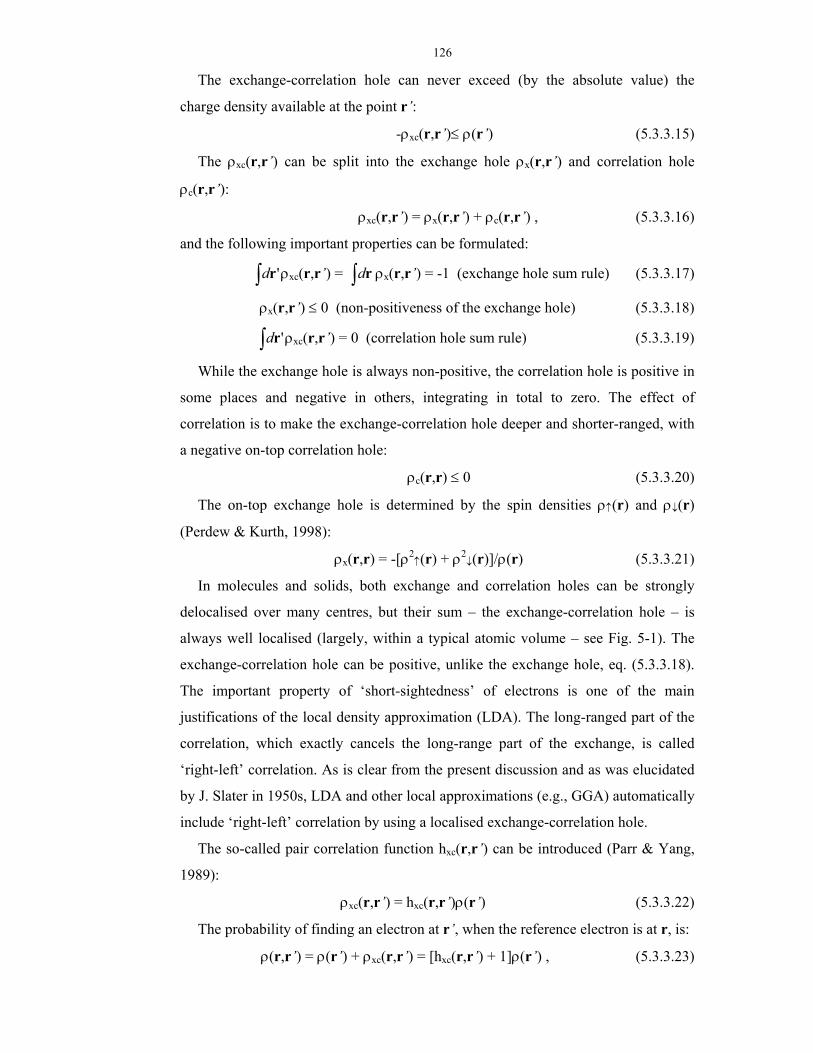
126
The exchange-correlation hole can never exceed (by the absolute value) the
charge density available at the point r’:
-ρxc(r,r’)≤ ρ(r’) (5.3.3.15)
The ρxc(r,r’) can be split into the exchange hole ρx(r,r’) and correlation hole
ρc(r,r’):
ρxc(r,r’) = ρx(r,r’) + ρc(r,r’) , (5.3.3.16)
and the following important properties can be formulated:
'∫ rd ρxc(r,r’) = ∫ rd ρx(r,r’) = -1 (exchange hole sum rule) (5.3.3.17)
ρx(r,r’) ≤ 0 (non-positiveness of the exchange hole) (5.3.3.18)
'∫ rd ρxc(r,r’) = 0 (correlation hole sum rule) (5.3.3.19)
While the exchange hole is always non-positive, the correlation hole is positive in
some places and negative in others, integrating in total to zero. The effect of
correlation is to make the exchange-correlation hole deeper and shorter-ranged, with
a negative on-top correlation hole:
ρc(r,r) ≤ 0 (5.3.3.20)
The on-top exchange hole is determined by the spin densities ρ↑(r) and ρ↓(r)
(Perdew & Kurth, 1998):
ρx(r,r) = -[ρ2↑(r) + ρ2
↓(r)]/ρ(r) (5.3.3.21)
In molecules and solids, both exchange and correlation holes can be strongly
delocalised over many centres, but their sum – the exchange-correlation hole – is
always well localised (largely, within a typical atomic volume – see Fig. 5-1). The
exchange-correlation hole can be positive, unlike the exchange hole, eq. (5.3.3.18).
The important property of ‘short-sightedness’ of electrons is one of the main
justifications of the local density approximation (LDA). The long-ranged part of the
correlation, which exactly cancels the long-range part of the exchange, is called
‘right-left’ correlation. As is clear from the present discussion and as was elucidated
by J. Slater in 1950s, LDA and other local approximations (e.g., GGA) automatically
include ‘right-left’ correlation by using a localised exchange-correlation hole.
The so-called pair correlation function hxc(r,r’) can be introduced (Parr & Yang,
1989):
ρxc(r,r’) = hxc(r,r’)ρ(r’) (5.3.3.22)
The probability of finding an electron at r’, when the reference electron is at r, is:
ρ(r,r’) = ρ(r’) + ρxc(r,r’) = [hxc(r,r’) + 1]ρ(r’) , (5.3.3.23)
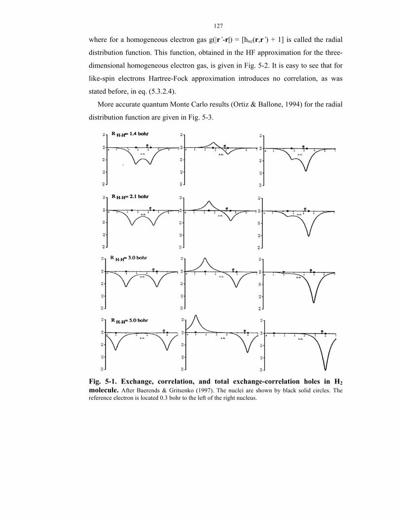
127
where for a homogeneous electron gas g(|r’-r|) = [hxc(r,r’) + 1] is called the radial
distribution function. This function, obtained in the HF approximation for the three-
dimensional homogeneous electron gas, is given in Fig. 5-2. It is easy to see that for
like-spin electrons Hartree-Fock approximation introduces no correlation, as was
stated before, in eq. (5.3.2.4).
More accurate quantum Monte Carlo results (Ortiz & Ballone, 1994) for the radial
distribution function are given in Fig. 5-3.
Fig. 5-1. Exchange, correlation, and total exchange-correlation holes in H2 molecule. After Baerends & Gritsenko (1997). The nuclei are shown by black solid circles. The reference electron is located 0.3 bohr to the left of the right nucleus.
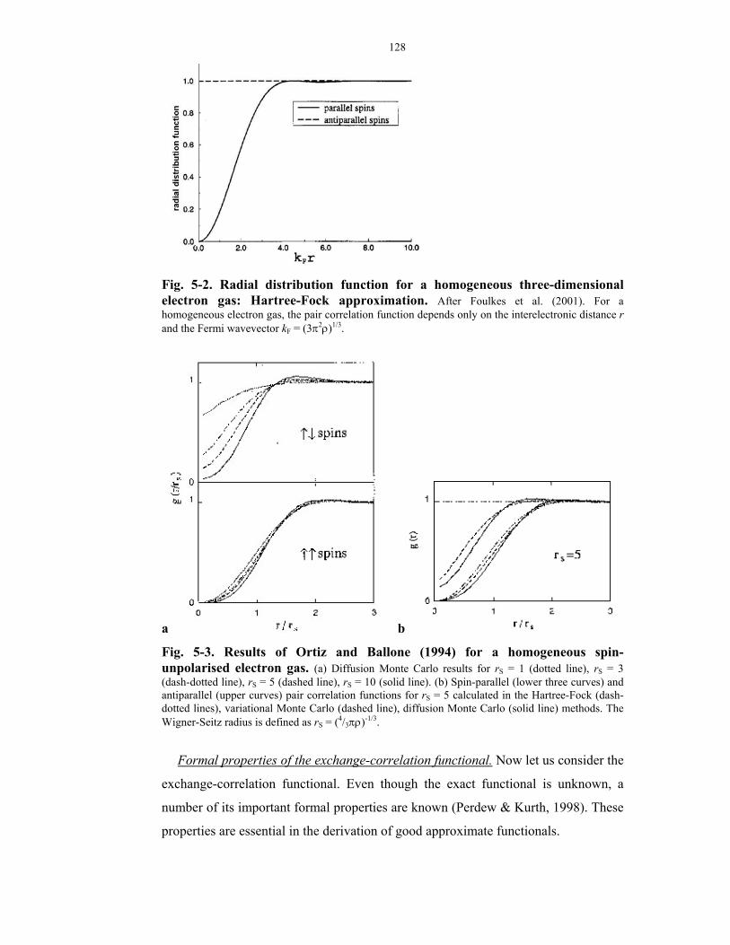
128
Fig. 5-2. Radial distribution function for a homogeneous three-dimensional electron gas: Hartree-Fock approximation. After Foulkes et al. (2001). For a homogeneous electron gas, the pair correlation function depends only on the interelectronic distance r and the Fermi wavevector kF = (3π2ρ)1/3.
a b
Fig. 5-3. Results of Ortiz and Ballone (1994) for a homogeneous spin-unpolarised electron gas. (a) Diffusion Monte Carlo results for rS = 1 (dotted line), rS = 3 (dash-dotted line), rS = 5 (dashed line), rS = 10 (solid line). (b) Spin-parallel (lower three curves) and antiparallel (upper curves) pair correlation functions for rS = 5 calculated in the Hartree-Fock (dash-dotted lines), variational Monte Carlo (dashed line), diffusion Monte Carlo (solid line) methods. The Wigner-Seitz radius is defined as rS = (4/3πρ)-1/3.
Formal properties of the exchange-correlation functional. Now let us consider the
exchange-correlation functional. Even though the exact functional is unknown, a
number of its important formal properties are known (Perdew & Kurth, 1998). These
properties are essential in the derivation of good approximate functionals.
129
First of all, the exchange energy is negative and correlation energy is non-
positive:
Ex[ρ] < 0 (5.3.3.24)
Ec[ρ] ≤ 0 (5.3.3.25)
Second, exact exchange completely corrects the self-interaction error. For any
one-electron system, exchange potential cancels the Hartree potential:
vx(r) 1=N = - vH(r) (5.3.3.26)
and there is no correlation in a one-electron system:
vc(r) 1=N = 0 (5.3.3.27)
Several exact uniform scaling properties are known. In such scaling, we replace
all the coordinates r with scaled coordinates γr. The density scales as:
ργ(r) = γ3ρ(r) (5.3.3.28)
For the Hartree energy [EH[ρ] = ½ ∫ rd ρ(r)vH(r)] the scaling is:
EH[ργ] = γEH[ρ] (5.3.3.29)
The kinetic energy of a non-interacting system scales as:
T[ργ] = γ2T[ρ] , (5.3.3.30)
and the scaling relation for the exchange energy is
Ex[ργ] = γEx[ρ] (5.3.3.31)
For the correlation energy, there exist the following scaling inequalities:
Ec[ργ] > γEc[ρ] (γ > 1)
Ec[ργ] < γEc[ρ] (γ < 1) (5.3.3.32)
A number of inequalities play an important role in DFT. The Lieb-Thirring
hypothesis states that the kinetic energy of a non-interacting system is greater than or
equal to the Thomas-Fermi esimate:
Ts[ρ] ≥ TTF[ρ] = 3/10(3π2)2/3 ∫ rd ρ5/3 (5.3.3.33)
Of special importance is the Lieb-Oxford bound for the exchange-correlation
energy:
|Exc[ρ]| ≤ 2.273|Ex,LDA[ρ]| = 2.273π43 (3π2)1/3 ∫ rd ρ4/3 (5.3.3.34)
We also know the exact spin scaling relations for the exchange energy:
Ex[ρ↑,ρ↓] = ½Ex[2ρ↑,0] + ½Ex[0,2ρ↓] (5.3.3.35)
and for the non-interacting kinetic energy:
TS[ρ↑,ρ↓] = ½TS[2ρ↑,0] + ½TS[0,2ρ↓] (5.3.3.36)
130
These relations play the central role in DFT for spin-polarised systems.
Unfortunately, there is no simple spin scaling relation for the correlation energy.
Other notations are useful, e.g. the spin density:
ρspin(r) = ρ↑(r) - ρ↓(r) (5.3.3.37)
and dimensionless spin polarisation ranging between 0 and 1:
ξ(r) = |ρ↑(r) - ρ↓(r)|/[ρ↑(r) + ρ↓(r)] (5.3.3.38)
It is possible to extend DFT to treat non-collinear magnetism (see Hobbs et al.,
2000 for a practical implementation).
As it was noted before, in exact DFT the highest-occupied eigenvalue is equal to
minus the ionisation potential of the system; it must change discontinuously at an
integer number Z of electrons:
εHO = (HOn
E∂∂ ) = -I (Z-1 < N < Z)
-A (Z < N < Z+1) , (5.3.3.39)
where I and A are the ionisation potential and electron affinity of the Z-electron
system (e.g., atom). The exchange-correlation potential has the following
asymptotical behaviour at r→∞:
vxc(r) → -||
1r
+ I + εHO , (5.3.3.40)
which reduces to -||
1r
for the exact functional. In approximate DFT the derivative
discontinuity (5.3.3.39) cannot be reproduced; instead, we approximately get
εHO ≈ -(I+A)/2 , (5.3.3.41)
which confers the meaning of minus the Mulliken electronegativity on the highest-
occupied eigenvalue εHO. Consequently, for the eigenvalue gap in (5.3.3.8) we have:
∆ε = (I - A2)/2 , (5.3.3.42)
where A2 is the affinity for the second electron, and the band gap is:
Eg = I - A , (5.3.3.43)
which gives the exchange-correlation correction ∆ in (5.3.3.8):
∆ = (I - 2A + A2)/2 (5.3.3.44)
5.3.4. Density functional theory (DFT) – approximate functionals.
In this section I shall expose some of the theory behind the most popular
approximate DFT methods. The performance of these methods is illustrated by the
131
comparison between different methods and experiment, demonstrated in Tables 5-1
to 5-5.
Local density approximation (LDA). LDA is the simplest approximation to Exc[ρ];
although the local expression (5.3.3.2) for the kinetic energy is very poor for atoms,
local exchange-correlation is rather accurate. In LDA, the kinetic energy is
calculated from orbitals using (5.3.3.4), rather that from the electron-gas formula
(5.3.3.2).
The exchange-correlation energy is calculated as:
Exc[ρ] = ∫ rd ρ(r)exc(ρ(r)) , (5.3.4.1)
where the exchange energy density of a homogeneous electron gas is known exactly
from (5.3.3.3):
ex(ρ) = -π43 (3π2)1/3ρ1/3 = -
π43 (9π/4)1/3rs
-1 , (5.3.4.2)
and the correlation energy density is known very accurately from quantum Monte
Carlo simulations of Ceperley and Alder (1980) and Ortiz and Ballone (1994). An
analytical representation satisfying the exactly known high- and low-density
analytical limits and fitting the numerical quantum Monte Carlo results for the spin-
unpolarised case, is (Perdew & Zunger, 1981):
ec(ρ) = 0.0311lnrs – 0.048 + 0.0020rslnrs – 0.0116rs (rs < 1),
ec(ρ) = -0.1423/(1 + 1.0529 sr + 0.3334rs) (rs > 1) (5.3.4.3)
Fig. 5-4 shows different contributions to the total energy of the homogeneous
electron gas and clearly indicates the importance of the correlation contribution.
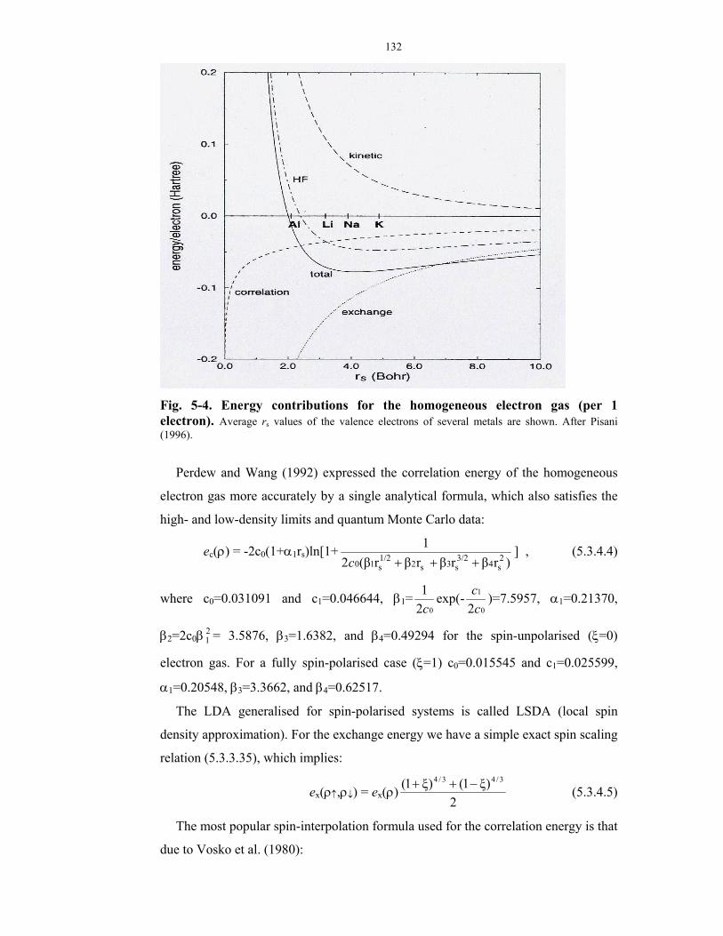
132
Fig. 5-4. Energy contributions for the homogeneous electron gas (per 1 electron). Average rs values of the valence electrons of several metals are shown. After Pisani (1996).
Perdew and Wang (1992) expressed the correlation energy of the homogeneous
electron gas more accurately by a single analytical formula, which also satisfies the
high- and low-density limits and quantum Monte Carlo data:
ec(ρ) = -2c0(1+α1rs)ln[1+)rβrβrβrβ(2
12s4
3/2s3s2
1/2s10 +++c
] , (5.3.4.4)
where c0=0.031091 and c1=0.046644, β1=02
1c
exp(-0
1
2cc )=7.5957, α1=0.21370,
β2=2c0β 21 = 3.5876, β3=1.6382, and β4=0.49294 for the spin-unpolarised (ξ=0)
electron gas. For a fully spin-polarised case (ξ=1) c0=0.015545 and c1=0.025599,
α1=0.20548, β3=3.3662, and β4=0.62517.
The LDA generalised for spin-polarised systems is called LSDA (local spin
density approximation). For the exchange energy we have a simple exact spin scaling
relation (5.3.3.35), which implies:
ex(ρ↑,ρ↓) = ex(ρ)2
)ξ1()ξ1( 3/43/4 −++ (5.3.4.5)
The most popular spin-interpolation formula used for the correlation energy is that
due to Vosko et al. (1980):
133
ec(ρ↑,ρ↓) = ec(ρ) + αc(ρ))ξ(f)ξ(f
'' (1-ξ4) + [ec(ρ,0)- ec(ρ)]f(ξ)ξ4 , (5.3.4.6)
where f(ξ)=22
2)1()1(3/4
3/43/4
−−−++ ξξ , and -αc(ρ) can be accurately represented by a
function of the type (5.3.4.4) with c0=0.016887, c1=0.035475, α1=0.11125,
β3=0.88026, β4=0.49671.
LDA leads to significant errors in exchange (about -5%) and correlation (about
+100%), but these largely cancel each other, explaining the successes of the LDA.
This approximation does not give accurate exchange-correlation holes for atoms, but
gives reasonable spherical averages for these holes – luckily, it is only the
spherically-symmetric part of the multipole expansion that is important. In addition,
and perhaps most importantly, LDA exactly satisfies all the sum rules (5.3.3.17) and
(5.3.3.19) that are true for the exact functional. The self-interaction error is largely
cancelled by the exchange-correlation potential; e.g., in the H atom ~95% of this
error is cancelled at the LSDA level of theory (Thijssen, 1999). However, this error
becomes important for highly localised electronic states (such as d-states in transition
metal atoms). Perdew and Zunger (1981) devised a simple method to incorporate the
self-interaction correction in the LDA approach (LDA+SIC). LDA+SIC offers a
significant improvement for atomic energies, but is difficult to apply to crystals,
where the electronic orbitals are usually represented by delocalised Bloch functions,
whose self-interaction is zero34.
The shortcomings of the LDA include the following: 1.Underestimation of the
energies of isolated atoms – LDA treats well the valence electrons, but significantly
underbinds the core electrons, 2. Overbinding (by ~20%) in molecules and crystals,
3. Bond lengths are usually ~1% too short, 4. Reaction barriers are usually too low
compared to experiment, 5. Large errors for weakly bonded systems (e.g., hydrogen
bonds), 6. van der Waals bonding cannot be treated correctly within the LDA, 7.
Sometimes the energy differences between polymorphs are inaccurate (e.g., for
quartz-stishovite the huge energy difference of ~0.5 eV is not reproduced: even the
sign is wrong!), 8. Often a wrong ground state is predicted (e.g., paramagnetic fcc
instead of ferromagnetic bcc for Fe), 9. Serious errors for many Mott insulators
(often magnetic moments are underestimated or low-spin states are predicted to be
34 In such cases, it is necessary to select and localise some orbitals (e.g., d- and f-orbitals of transition
metal ions) – see Szotek & Temmerman (1993) for details and application to transition metal oxides.
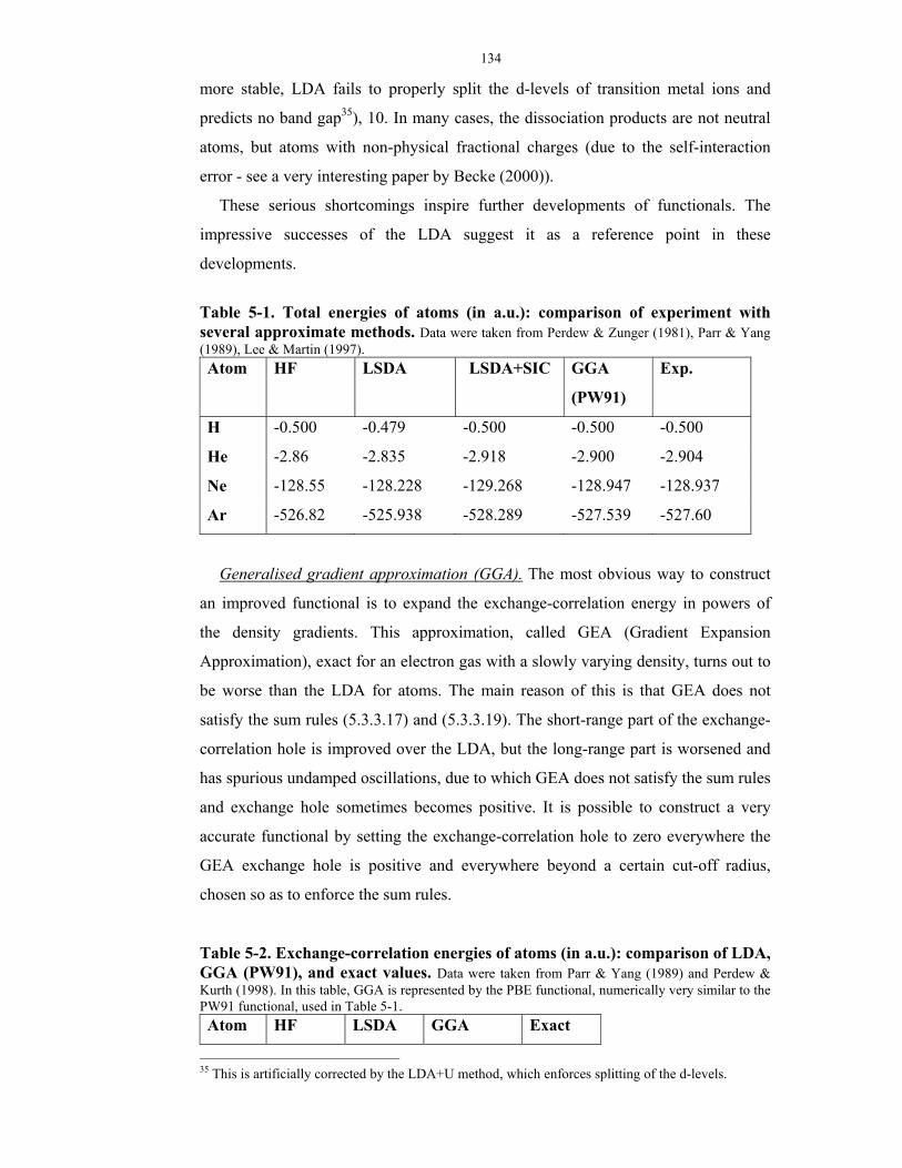
134
more stable, LDA fails to properly split the d-levels of transition metal ions and
predicts no band gap35), 10. In many cases, the dissociation products are not neutral
atoms, but atoms with non-physical fractional charges (due to the self-interaction
error - see a very interesting paper by Becke (2000)).
These serious shortcomings inspire further developments of functionals. The
impressive successes of the LDA suggest it as a reference point in these
developments.
Table 5-1. Total energies of atoms (in a.u.): comparison of experiment with several approximate methods. Data were taken from Perdew & Zunger (1981), Parr & Yang (1989), Lee & Martin (1997). Atom HF LSDA LSDA+SIC GGA
(PW91)
Exp.
H -0.500 -0.479 -0.500 -0.500 -0.500
He -2.86 -2.835 -2.918 -2.900 -2.904
Ne -128.55 -128.228 -129.268 -128.947 -128.937
Ar -526.82 -525.938 -528.289 -527.539 -527.60
Generalised gradient approximation (GGA). The most obvious way to construct
an improved functional is to expand the exchange-correlation energy in powers of
the density gradients. This approximation, called GEA (Gradient Expansion
Approximation), exact for an electron gas with a slowly varying density, turns out to
be worse than the LDA for atoms. The main reason of this is that GEA does not
satisfy the sum rules (5.3.3.17) and (5.3.3.19). The short-range part of the exchange-
correlation hole is improved over the LDA, but the long-range part is worsened and
has spurious undamped oscillations, due to which GEA does not satisfy the sum rules
and exchange hole sometimes becomes positive. It is possible to construct a very
accurate functional by setting the exchange-correlation hole to zero everywhere the
GEA exchange hole is positive and everywhere beyond a certain cut-off radius,
chosen so as to enforce the sum rules.
Table 5-2. Exchange-correlation energies of atoms (in a.u.): comparison of LDA, GGA (PW91), and exact values. Data were taken from Parr & Yang (1989) and Perdew & Kurth (1998). In this table, GGA is represented by the PBE functional, numerically very similar to the PW91 functional, used in Table 5-1. Atom HF LSDA GGA Exact
35 This is artificially corrected by the LDA+U method, which enforces splitting of the d-levels.

135
(PBE)
H -0.31 -0.29 -0.31 -0.31
He -1.03 -1.00 -1.06 -1.09
Li -1.78 -1.69 -1.81 -1.83
Ne -12.11 -11.78 -12.42 -12.50
GGA is constructed in such a way as to preserve all the correct features of the
LDA and add some more. There are several popular GGA functionals, the best of
which seem to be the PW91 functional (Wang & Perdew, 1991) and a very similar
functional PBE (Perdew et al., 1996) – below I will mainly describe their features.
Good GGA exchange-correlation functionals satisfy several conditions:
• Reduce to GEA for slowly varying densities.
• Reduce to LDA for the homogeneous electron gas.
• Satisfy sum rules (5.3.3.17) and (5.3.3.19).
• Satisfy conditions (5.3.3.15,18,20).
• Have proper scaling (5.3.3.31,32).
• Have proper spin scaling (5.3.3.35).
• Obey the Lieb-Oxford bound (5.3.3.34).
GGA exchange is defined as:
Ex[ρ,∇ρ] = ∫ rd Fx(s)ρ(r)ex(ρ(r)) , (5.3.4.7)
where ex(ρ(r)) is the exchange energy of the homogeneous electron gas per 1
electron (given by (5.3.5.1)), and the exchange enhancement factor Fx(s) is a
function of the reduced density gradient s:
s = )(ρ)2(3
|ρ|4/31/3 rπ
∇ = )(ρ2
|ρ|
F rk∇ (5.3.4.8)
Set in this form, GGA exchange automatically has the correct scaling behaviour
(5.3.3.31). For the total exchange-correlation functional the definition is:
Exc[ρ,∇ρ] = ∫ rd Fxc(ρ,s)ρ(r)ex(ρ(r)) 36 , (5.3.4.9)
where the enhancement factor Fxc(ρ,s) now depends on both the density and its
reduced gradient. No GGA functional is expected to be accurate for s>>1; happily,
36 For spin-polarised cases, Exc[ρ,ξ,∇ρ] = ∫ rd Fxc(ρ,ξ,s)ρ(r)ex(ρ(r)).
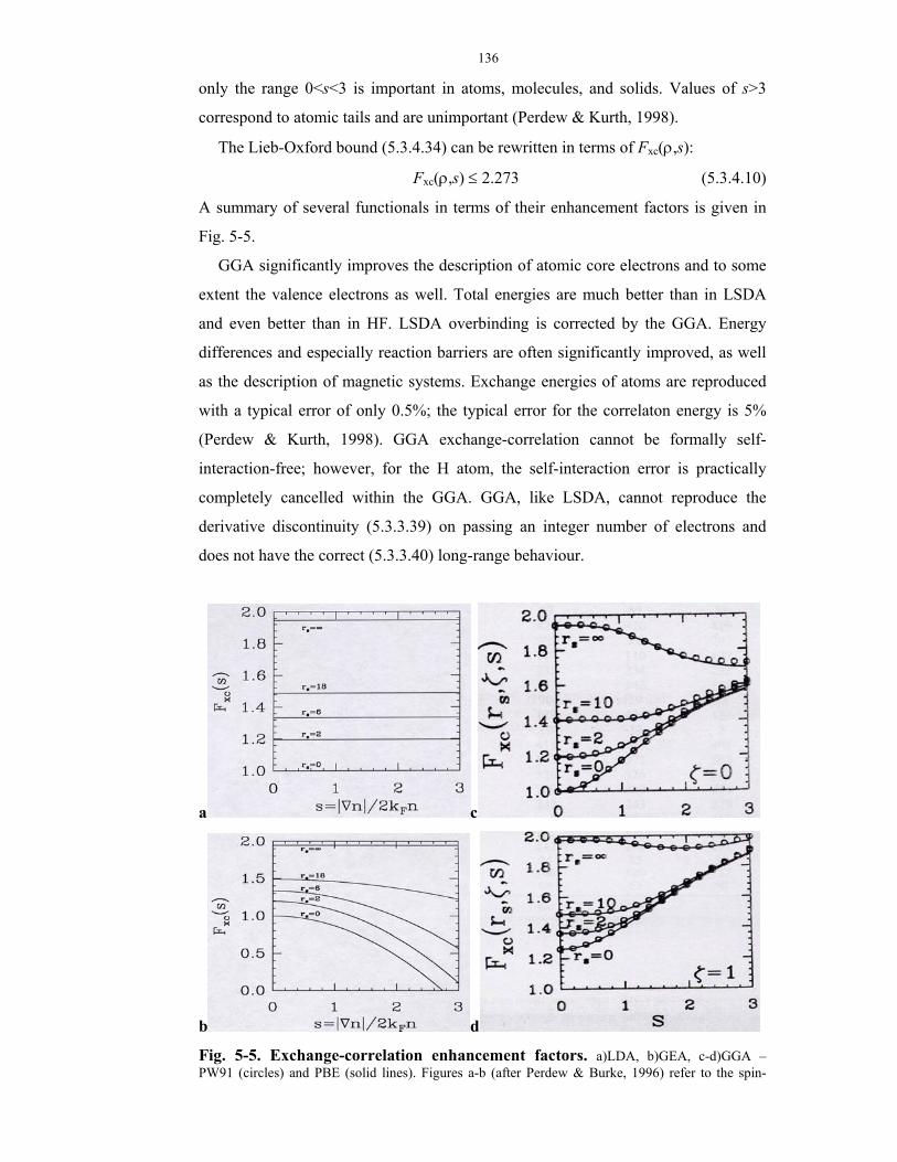
136
only the range 0<s<3 is important in atoms, molecules, and solids. Values of s>3
correspond to atomic tails and are unimportant (Perdew & Kurth, 1998).
The Lieb-Oxford bound (5.3.4.34) can be rewritten in terms of Fxc(ρ,s):
Fxc(ρ,s) ≤ 2.273 (5.3.4.10)
A summary of several functionals in terms of their enhancement factors is given in
Fig. 5-5.
GGA significantly improves the description of atomic core electrons and to some
extent the valence electrons as well. Total energies are much better than in LSDA
and even better than in HF. LSDA overbinding is corrected by the GGA. Energy
differences and especially reaction barriers are often significantly improved, as well
as the description of magnetic systems. Exchange energies of atoms are reproduced
with a typical error of only 0.5%; the typical error for the correlaton energy is 5%
(Perdew & Kurth, 1998). GGA exchange-correlation cannot be formally self-
interaction-free; however, for the H atom, the self-interaction error is practically
completely cancelled within the GGA. GGA, like LSDA, cannot reproduce the
derivative discontinuity (5.3.3.39) on passing an integer number of electrons and
does not have the correct (5.3.3.40) long-range behaviour.
a c
b d
Fig. 5-5. Exchange-correlation enhancement factors. a)LDA, b)GEA, c-d)GGA – PW91 (circles) and PBE (solid lines). Figures a-b (after Perdew & Burke, 1996) refer to the spin-
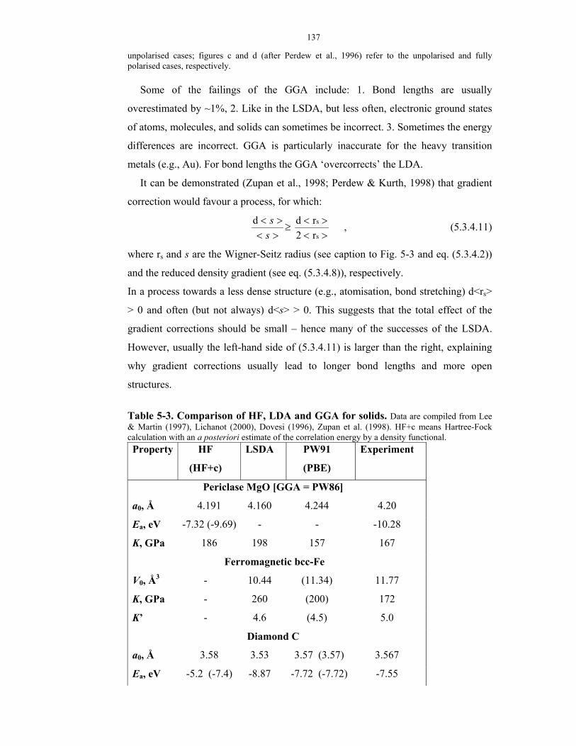
137
unpolarised cases; figures c and d (after Perdew et al., 1996) refer to the unpolarised and fully polarised cases, respectively.
Some of the failings of the GGA include: 1. Bond lengths are usually
overestimated by ~1%, 2. Like in the LSDA, but less often, electronic ground states
of atoms, molecules, and solids can sometimes be incorrect. 3. Sometimes the energy
differences are incorrect. GGA is particularly inaccurate for the heavy transition
metals (e.g., Au). For bond lengths the GGA ‘overcorrects’ the LDA.
It can be demonstrated (Zupan et al., 1998; Perdew & Kurth, 1998) that gradient
correction would favour a process, for which:
><><
ssd
≥ ><><
s
s
r2rd , (5.3.4.11)
where rs and s are the Wigner-Seitz radius (see caption to Fig. 5-3 and eq. (5.3.4.2))
and the reduced density gradient (see eq. (5.3.4.8)), respectively.
In a process towards a less dense structure (e.g., atomisation, bond stretching) d<rs>
> 0 and often (but not always) d<s> > 0. This suggests that the total effect of the
gradient corrections should be small – hence many of the successes of the LSDA.
However, usually the left-hand side of (5.3.4.11) is larger than the right, explaining
why gradient corrections usually lead to longer bond lengths and more open
structures.
Table 5-3. Comparison of HF, LDA and GGA for solids. Data are compiled from Lee & Martin (1997), Lichanot (2000), Dovesi (1996), Zupan et al. (1998). HF+c means Hartree-Fock calculation with an a posteriori estimate of the correlation energy by a density functional. Property HF
(HF+c)
LSDA PW91
(PBE)
Experiment
Periclase MgO [GGA = PW86]
a0, Å 4.191 4.160 4.244 4.20
Ea, eV -7.32 (-9.69) - - -10.28
K, GPa 186 198 157 167
Ferromagnetic bcc-Fe
V0, Å3 - 10.44 (11.34) 11.77
K, GPa - 260 (200) 172
K’ - 4.6 (4.5) 5.0
Diamond C
a0, Å 3.58 3.53 3.57 (3.57) 3.567
Ea, eV -5.2 (-7.4) -8.87 -7.72 (-7.72) -7.55

138
K, GPa 471 455 438 (439) 442
Table 5-4. Comparison between LSDA, LDA+U, GGA, and experiment for antiferromagnetic FeO. Data are taken from Isaak et al. (1993), Cohen et al. (1997), Fang et al. (1999), Gramsch et al. (2001).
LSDA LDA+U GGA Experiment
V0, Å3 141.5 161.2 165.8, 156.8, 157.1 162.82
K, GPa 173 186 178, 180, 158 142-180
K’ 4.3 3.43 4.2, 3.55, 3.05 4.9
µFe 3.4 3.4 -, 3.46, 3.5 4.2
Notes: 1. The ground state of FeO at 0 K is rhombohedral antiferromagnetic; however, the Neél temperature of FeO (198 K) is below room temperature and most experiments refer to the spin-disordered cubic phase. This is a different phase, whose properties are, however, similar. 2. The LSDA entry for the volume is ambiguous: Isaak et al. (1993) give only the lattice parameter, which they seem to define as the cubic root of the volume of the rhombohedrally distorted cell. 3. Experimental magnetic moments of Fe atoms have a large orbital component, which is not included in usual calculations. For the spin magnetic moments agreement between theory and experiment is good.
Meta-GGA. The next step after GGA is to include the Laplacian of the electron
density ∇2ρ. The inclusion of this variable is very promising, since the Laplacian of
the density proved to be very important in the Bader analysis of chemical bonding
(Bader, 1990; Coppens, 1997; Tsirelson, 1993). Quantum Monte Carlo simulations
(Nekovee et al., 2001) demonstrated that often GGA would worsen the LDA
exchange-correlation hole. They also showed that inclusion of the Laplacian of the
density is essential in reasonable modelling of the exact hole. There have been
several attempts to construct meta-GGA functionals. E.g., Perdew et al. (1999) have
constructed a meta-GGA functional including the Laplacian of the density and the
kinetic energy density, which is defined as:
τ(r) = ½Σ∇ 2φi(r) (5.3.4.12)
Table 5-5. Atomisation energies (in eV) of several molecules: experiment versus theory. Experimental values include a correction for zero-point vibrational energy. All calculations are spin-polarised. (Taken from Perdew et al., 1996; meta-GGA results: from Perdew et al., 1999). Meta-GGA calculations used GGA electron densities.
Molecule HF LSDA GGA
(PBE)
GGA
(PW91)
Meta-GGA Experiment
H2 3.64 4.90 4.55 4.55 4.97 4.73
OH 2.95 5.38 4.77 4.77 4.67 4.64
H2O 6.72 11.58 10.15 10.19 9.98 10.06
HF 4.21 7.03 6.16 6.20 6.01 6.11
Li2 0.09 1.00 0.82 0.87 0.98 1.04
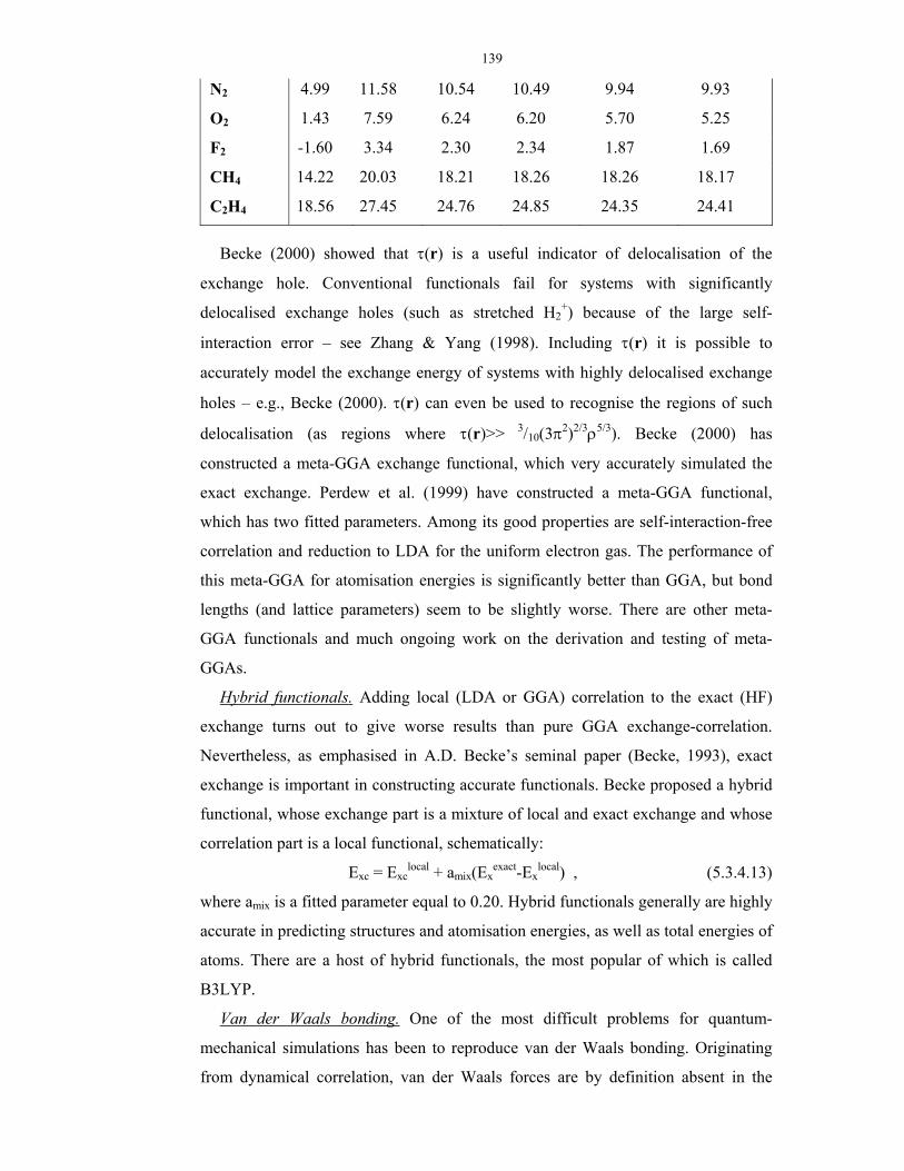
139
N2 4.99 11.58 10.54 10.49 9.94 9.93
O2 1.43 7.59 6.24 6.20 5.70 5.25
F2 -1.60 3.34 2.30 2.34 1.87 1.69
CH4 14.22 20.03 18.21 18.26 18.26 18.17
C2H4 18.56 27.45 24.76 24.85 24.35 24.41 Becke (2000) showed that τ(r) is a useful indicator of delocalisation of the
exchange hole. Conventional functionals fail for systems with significantly
delocalised exchange holes (such as stretched H2+) because of the large self-
interaction error – see Zhang & Yang (1998). Including τ(r) it is possible to
accurately model the exchange energy of systems with highly delocalised exchange
holes – e.g., Becke (2000). τ(r) can even be used to recognise the regions of such
delocalisation (as regions where τ(r)>> 3/10(3π2)2/3ρ5/3). Becke (2000) has
constructed a meta-GGA exchange functional, which very accurately simulated the
exact exchange. Perdew et al. (1999) have constructed a meta-GGA functional,
which has two fitted parameters. Among its good properties are self-interaction-free
correlation and reduction to LDA for the uniform electron gas. The performance of
this meta-GGA for atomisation energies is significantly better than GGA, but bond
lengths (and lattice parameters) seem to be slightly worse. There are other meta-
GGA functionals and much ongoing work on the derivation and testing of meta-
GGAs.
Hybrid functionals. Adding local (LDA or GGA) correlation to the exact (HF)
exchange turns out to give worse results than pure GGA exchange-correlation.
Nevertheless, as emphasised in A.D. Becke’s seminal paper (Becke, 1993), exact
exchange is important in constructing accurate functionals. Becke proposed a hybrid
functional, whose exchange part is a mixture of local and exact exchange and whose
correlation part is a local functional, schematically:
Exc = Exclocal + amix(Ex
exact-Exlocal) , (5.3.4.13)
where amix is a fitted parameter equal to 0.20. Hybrid functionals generally are highly
accurate in predicting structures and atomisation energies, as well as total energies of
atoms. There are a host of hybrid functionals, the most popular of which is called
B3LYP.
Van der Waals bonding. One of the most difficult problems for quantum-
mechanical simulations has been to reproduce van der Waals bonding. Originating
from dynamical correlation, van der Waals forces are by definition absent in the
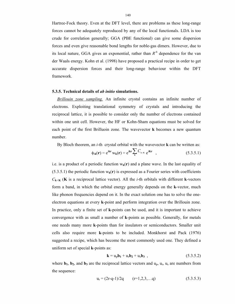
140
Hartree-Fock theory. Even at the DFT level, there are problems as these long-range
forces cannot be adequately reproduced by any of the local functionals. LDA is too
crude for correlation generally; GGA (PBE functional) can give some dispersion
forces and even give reasonable bond lengths for noble-gas dimers. However, due to
its local nature, GGA gives an exponential, rather than R-6 dependence for the van
der Waals energy. Kohn et al. (1998) have proposed a practical recipe in order to get
accurate dispersion forces and their long-range behaviour within the DFT
framework.
5.3.5. Technical details of ab initio simulations.
Brillouin zone sampling. An infinite crystal contains an infinite number of
electrons. Exploiting translational symmetry of crystals and introducing the
reciprocal lattice, it is possible to consider only the number of electrons contained
within one unit cell. However, the HF or Kohn-Sham equations must be solved for
each point of the first Brilluoin zone. The wavevector k becomes a new quantum
number.
By Bloch theorem, an i-th crystal orbital with the wavevector k can be written as:
φik(r) = eikr wk(r) = eikr ∑ +K
KkC eiKr , (5.3.5.1)
i.e. is a product of a periodic function wk(r) and a plane wave. In the last equality of
(5.3.5.1) the periodic function wk(r) is expressed as a Fourier series with coefficients
Ck+K (K is a reciprocal lattice vector). All the i-th orbitals with different k-vectors
form a band, in which the orbital energy generally depends on the k-vector, much
like phonon frequencies depend on it. In the exact solution one has to solve the one-
electron equations at every k-point and perform integration over the Brillouin zone.
In practice, only a finite set of k-points can be used, and it is important to achieve
convergence with as small a number of k-points as possible. Generally, for metals
one needs many more k-points than for insulators or semiconductors. Smaller unit
cells also require more k-points to be included. Monkhorst and Pack (1976)
suggested a recipe, which has become the most commonly used one. They defined a
uniform set of special k-points as:
k = upb1 + urb2 + usb3 , (5.3.5.2)
where b1, b2, and b3 are the reciprocal lattice vectors and up, ur, us are numbers from
the sequence:
ur = (2r-q-1)/2q (r=1,2,3,…q) (5.3.5.3)

141
The total number of k-points is q3, but due to symmetry the number of independent
k-points can be much smaller.
Basis sets. Here I shall consider only the traditional atomic-orbital and plane wave
basis sets. There exist other possibilities, e.g. hybrid basis sets of the LAPW method.
In the LCAO (Linear Combination of Atomic Orbitals) scheme one defines atom-
centred orbitals as a product of the angular (Ylm) and radial (χ(r)) parts:
φi(r) = Ylmχ(|r|) , (5.3.5.4)
where the radial part is a linear combination of either Slater-type functions:
χ(|r|) = rme-ξr (5.3.5.5)
or Gaussian-type functions:
χ(|r|) = e r 2α− , (5.3.5.6)
where m, ξ, and α are parameters. Slater orbitals are more accurate and require fewer
functions in an accurate representation of orbitals. However, they are much more
computationally expensive, and Gaussian functions are usually preferred.
From atomic orbitals we form a set of Bloch functions, whose linear combinations
give the crystal orbitals. In practice, LCAO basis sets almost always suffer from
incompleteness. In molecules and crystals, parameters (e.g., exponents) of the
orbitals (5.3.5.5) and (5.3.5.6) depend on the atomic positions, but are only optimised
for one structure. Dependence of the basis set on atomic positions implies the
presence of Pulay forces, which must be evaluated when optimising crystal
structures. Although very economical for insulators, LCAO basis needs very many
Gaussian functions for studies of metals. LCAO basis also suffers from the basis set
superposition error. It is also difficult to systematically increase the basis set
expressed in local orbitals.
Plane wave basis set is the most natural and general basis set for crystals,
following directly from the Bloch theorem. A single plane wave is:
φ PWKk+ (r) = ei(k+K)r (5.3.5.7)
This basis set is complete and very convenient for many applications. Its main
shortcoming is that a huge number of plane waves are needed to describe rapidly
changing wavefunctions in solids. E.g., for the valence electrons in Al, an estimated
106 plane waves are needed to reproduce oscillations of the valence electron
wavefunction in the core region. For the core electrons this problem is even much
more serious – because the core electron wavefunctions are more rapidly changing
and there is a cusp in the density (eq. 5.3.4) at the nucleus. There are several ways to
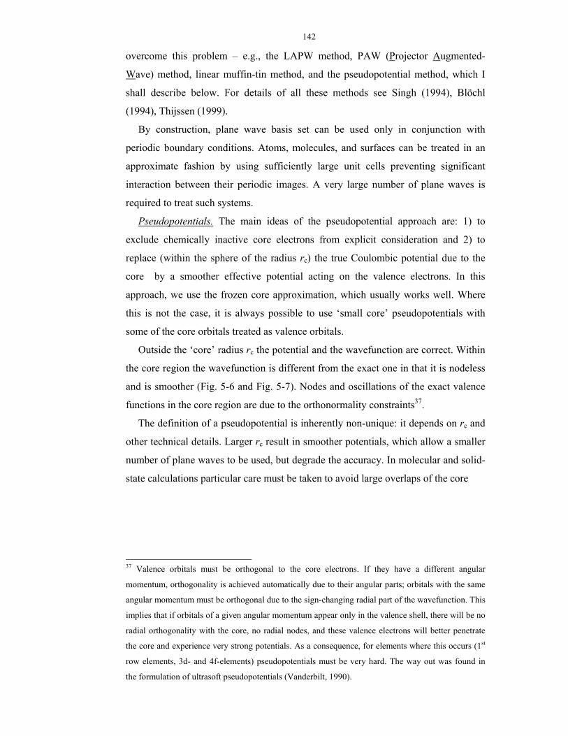
142
overcome this problem – e.g., the LAPW method, PAW (Projector Augmented-
Wave) method, linear muffin-tin method, and the pseudopotential method, which I
shall describe below. For details of all these methods see Singh (1994), Blöchl
(1994), Thijssen (1999).
By construction, plane wave basis set can be used only in conjunction with
periodic boundary conditions. Atoms, molecules, and surfaces can be treated in an
approximate fashion by using sufficiently large unit cells preventing significant
interaction between their periodic images. A very large number of plane waves is
required to treat such systems.
Pseudopotentials. The main ideas of the pseudopotential approach are: 1) to
exclude chemically inactive core electrons from explicit consideration and 2) to
replace (within the sphere of the radius rc) the true Coulombic potential due to the
core by a smoother effective potential acting on the valence electrons. In this
approach, we use the frozen core approximation, which usually works well. Where
this is not the case, it is always possible to use ‘small core’ pseudopotentials with
some of the core orbitals treated as valence orbitals.
Outside the ‘core’ radius rc the potential and the wavefunction are correct. Within
the core region the wavefunction is different from the exact one in that it is nodeless
and is smoother (Fig. 5-6 and Fig. 5-7). Nodes and oscillations of the exact valence
functions in the core region are due to the orthonormality constraints37.
The definition of a pseudopotential is inherently non-unique: it depends on rc and
other technical details. Larger rc result in smoother potentials, which allow a smaller
number of plane waves to be used, but degrade the accuracy. In molecular and solid-
state calculations particular care must be taken to avoid large overlaps of the core
37 Valence orbitals must be orthogonal to the core electrons. If they have a different angular
momentum, orthogonality is achieved automatically due to their angular parts; orbitals with the same
angular momentum must be orthogonal due to the sign-changing radial part of the wavefunction. This
implies that if orbitals of a given angular momentum appear only in the valence shell, there will be no
radial orthogonality with the core, no radial nodes, and these valence electrons will better penetrate
the core and experience very strong potentials. As a consequence, for elements where this occurs (1st
row elements, 3d- and 4f-elements) pseudopotentials must be very hard. The way out was found in
the formulation of ultrasoft pseudopotentials (Vanderbilt, 1990).
143
Fig. 5-6. Construction of a pseudopotential. Beyond rc the wavefunction and potential match the true all-electron ones (with modifications after Payne et al., 1992).
a b Fig. 5-7. All-electron (a) and pseudowavefunction (b) of a 5d-orbital in Au. Solid contours – positive, dashed contours – negative wavefinction (taken from A. Rappe’s web-page at: http://www.sas.upenn.edu/chem/faculty/rappe/rappe.html).
regions. At rc not only the wavefunction, but also its first derivative are exact,
therefore small overlaps are not critical. Pseudopotentials are constructed so as to
match the all-electron eigenvalues in as many different atomic configurations as
possible, to ensure transferability of the pseudopotential to chemically different
systems.
Usually, pseudopotentials are generated under a constraint of norm-conservation:
∑ ∫ φi
psrc
rr d|)(| 2
0i = ∑ ∫ φ
i
aerc
rr d|)(| 2
0i , (5.3.5.8)
i.e. the pseudowavefunction gives the correct (equal to the all-electron result)
number of valence electrons within the core region. These pseudopotentials are
called hard, or norm-conserving. It is possible to use much softer pseudopotentials
144
(called ultrasoft, or non-normconserving) by relaxing the norm-conservation
condition (Vanderbilt, 1990). This allows one to use relatively large rc and reduce the
number of plane waves by a factor of ~2 without any loss in accuracy. In Vanderbilt
pseudopotentials, one has to add the so called ‘augmentation charge’ (which is the
strongly atom-localised part of the valence electron density) to ∑i
| psiφ (r)|2 in order
to obtain the charge density within the core spheres. Ultrasoft pseudopotentials are
almost indispensable in simulations of compounds of ‘hard’ elements – such as O
and other 1st row elements, Fe and other 3d-elements, and rare earths.
Milman and co-workers (2000) have presented an analysis of the performance of
plane wave pseudopotential calculations for compounds of almost all elements.
Comparison of the performance of pseudopotential and all-electron methods was
made in many works, e.g. Holzwarth et al. (1997). The general conclusion is that
pseudopotential calculations are very accurate, except in cases where core
polarisation effects are significant (e.g., Ca atom in CaF2). Another source of errors
of pseudopotential calculations is significant overlap of the valence and core orbitals
for some elements (e.g., Na). In such cases, non-linear core corrections (Louie et al.,
1982) significantly improve pseudopotentials. It is important that the same functional
is used in generating the pseudopotential and in performing solid-state calculations
(Fuchs et al., 1998); this point, not taken into account by many researchers, was
always kept in my works, all of which used the PW91 functional for both solid-state
calculations and pseudopotential generation.
In conjunction with pseudopotentials, plane wave basis sets become extremely
useful. Using ultrasoft pseudopotentials, it is possible to give a satisfactory
description of solids by using typically a basis set of ~100 plane waves per atom.
Only the plane waves with the lowest kinetic energy need to be included. The
number of plane waves is controlled by the kinetic energy cut-off parameter Ecut;
only plane waves with the kinetic energy below Ecut are included:
21 |k+K|2 ≤ Ecut (in atomic units) (5.3.5.9)
The number of plane waves is roughly proportional to the volume of the unit cell
and depends on the cut-off as E 3/2cut ; an approximate estimate of the number of plane
waves:
Nc= 26πV (2Ecut)3/2 (5.3.5.10)
145
differs only slightly from the actual number Na. It must be always checked that Ecut is
high enough for good convergence of results.
A plane wave basis set does not depend on atomic positions; therefore, there are
no Pulay forces. However, this basis does depend on the volume when a finite
number of plane waves are included38. This is the origin of the so-called Pulay stress.
This stress is always negative, i.e. tends to compress the structure. It is nearly
isotropic, has zero shear components and is roughly independent of volume:
σp = cutE
EV ln32
∂∂ , (5.3.5.11)
Pulay stress affects mainly the pressure, which can be easily corrected by shifting
the calculated values by a constant:
p(V) = pN(V) + σp , (5.3.5.12)
where pN is the pressure calculated at the constant number of plane waves. The origin
of the Pulay stress is in the basis set incompleteness due to the presence of only a
finite number of plane waves. A related correction to the total energy (Francis &
Payne, 1990) is:
Etot = Etot(N) - c
a
cut NN
EE ln
ln32
∂∂ (5.3.5.13)
Increasing the basis set, it is possible to reduce the Pulay stress and errors in the
total energy to arbitrarily small values; all my calculations have negligible Pulay
stresses and very small total energy errors avoiding the use of the approximate
equations (5.3.5.11-13). For more details of the plane wave pseudopotential method
see Singh (1994) and Payne et al. (1992).
Fig. 5-8 presents valence electron distributions calculated using this method.
Analysis of the charge and spin densities is a powerful tool for investigation of
chemical bonding and interatomic interactions in crystals (Coppens, 1992, 1997;
Tsirelson, 1986, 1993). Figure 5-8 already gives some indication of the ionicity of
bonds and degree of charge transfer. More quantitative information can be obtained
by integration of the charge density within a sphere and comparison of results
obtained for different systems. This is shown in Fig. 5-9.
Existing programs for crystals. A number of codes based on DFT exist for
crystals. Plane-wave pseudopotential codes include VASP, CPMD, CASTEP,
CETEP, PWSCF, DoD-Planewave, ABINIT. WIEN is an all-electron code based on 38 There are even discontinuities in the basis set related to volume change during structural
optimisation. Such effects are significantly reduced when working with large sets of plane waves.
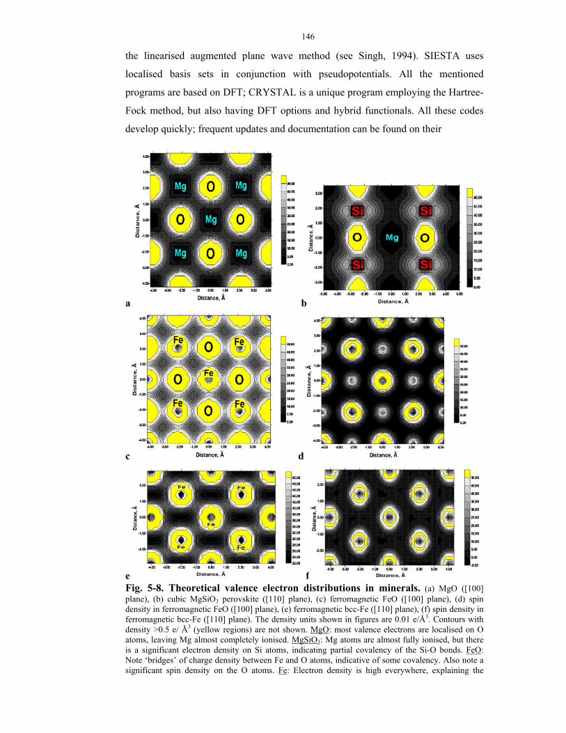
146
the linearised augmented plane wave method (see Singh, 1994). SIESTA uses
localised basis sets in conjunction with pseudopotentials. All the mentioned
programs are based on DFT; CRYSTAL is a unique program employing the Hartree-
Fock method, but also having DFT options and hybrid functionals. All these codes
develop quickly; frequent updates and documentation can be found on their
a b
c d
e f Fig. 5-8. Theoretical valence electron distributions in minerals. (a) MgO ([100] plane), (b) cubic MgSiO3 perovskite ([110] plane), (c) ferromagnetic FeO ([100] plane), (d) spin density in ferromagnetic FeO ([100] plane), (e) ferromagnetic bcc-Fe ([110] plane), (f) spin density in ferromagnetic bcc-Fe ([110] plane). The density units shown in figures are 0.01 e/Å3. Contours with density >0.5 e/ Å3 (yellow regions) are not shown. MgO: most valence electrons are localised on O atoms, leaving Mg almost completely ionised. MgSiO3: Mg atoms are almost fully ionised, but there is a significant electron density on Si atoms, indicating partial covalency of the Si-O bonds. FeO: Note ‘bridges’ of charge density between Fe and O atoms, indicative of some covalency. Also note a significant spin density on the O atoms. Fe: Electron density is high everywhere, explaining the

147
metallic conductivity of iron. In the ferromagnetic phase, the spin density is localised on the atoms and is positive everywhere, perhaps except for small interstitial regions where it is slightly negative. Calculations were performed using GGA-PW91 and VASP. Lev00 code (Kantorovich, 1996-2001) was used in constructing these images. Experimental structures were used for MgO (a0 = 4.211 Å) and Fe (a0 = 2.866 Å) and theoretical structure (a0=3.527 Å) was used for the cubic MgSiO3 perovskite. For FeO calculations, a0 = 4.211 Å was used for comparison with MgO.
a b
c d Fig. 5-9. Amount of charge inside atomic spheres in mineral structures. (a) in MgSiO3 perovskite, (b) Mg in MgO and MgSiO3 perovskite, (c) O in MgO, MgSiO3, and FeO, (d) Fe in FeO and metallic Fe. Arrows show the ionic radii (0.72 Å for Mg2+ and 1.40 Å for O2-, 0.40 Å for Si4+, and 0.78 Å for the high-spin Fe2+). Integrating charge within the spheres with these radii gives the atomic charges of Mg (+1.94 in MgO, +1.96 in MgSiO3), Si (+3.98), Fe (+3.27 in FeO and Fe), and O (–1.4 in MgO, -1.88 in MgSiO3, -2.00 in FeO). These figures, based on the same calculations as Fig. 5-8, show that: 1) atoms have nearly formal charges within the ionic radius spheres, 2) the sum of thus determined charges is not zero, because of the interstitial regions, 3) there is a striking difference between charge distributions around Mg in MgO and MgSiO3 and a striking similarity between charge distributions around the Fe atom in both Fe metal and FeO. The latter lends some support to the model of a metal as a system of ionic cores immersed in the sea of the free electrons; FeO is an ionic compound. The horizontal line in (c) indicates the full ionic charge. These images were created using the Lev00 code (Kantorovich, 1996-2001).
web-pages, which can be accessed from my home page
http://slamdunk.geol.ucl.ac.uk/~artem/7.html).
VASP (Vienna Ab initio Simulation Package: Kresse & Furthmüller, 1996a,b)
code is the main tool used in my work. It is based on DFT within the plane wave
pseudopotentials method, and has both static and molecular dynamics regimes. There
are numerous options of static structural relaxation in VASP, the most robust of
148
which is the conjugate gradients method (see Payne et al., 1992). For studies of
metals, a number of ‘smearing’ methods are available, in which an electronic
temperature is specified and the electronic entropy is computed from the density of
states. Molecular dynamics can be performed with VASP only in the NVE and NVT
ensembles. Equations of motion are solved using the Verlet algorithm; the constant-
temperature molecular dynamics is based on the method of Nosé (1984). The
program uses pseudopotentials of several types (including the ultrasoft ones), very
efficient matrix diagonalisation and charge density mixing algorithms; it is very
effectively parallelised, and can be used to study relatively large systems.
Pseudopotentials are generated by a scalar relativistic code; a library of
pseudopotentials for all elements is available.
5.3.6. Semiclassical simulations.
These are based on the methods developed by M. Born and co-workers (Born &
Huang, 1954). Computationallly much less expensive than ab initio calculations,
semiclassical simulations allow very large and complex systems, defects, and
dynamics to be studied.
Any potential energy hypersurface in principle can be represented analytically.
Knowing the whole potential energy surface, one can calculate the equilibrium
structure, its dynamics, all responses to the temperature and stress (e.g., elastic
constants, thermal expansion), defect properties, diffusion coefficients, vibrational
spectra, thermodynamic properties, melting curves, etc. See (Catlow et al., 1994) for
a good review. The only class of phenomena that cannot be calculated even in
principle is the electronic properties (e.g., magnetic structures, excitation energies),
which are entirely in the domain of ab initio methods. The Kohn anomalies in
phonon dispersion curves of metals also cannot be reproduced by semiclassical
methods. Generally, there are practical difficulties for metals, compounds with
electronic effects (e.g., Jahn-Teller effect, lone electron pairs)39 and difficulties in
situations where the bonds form, break, or significantly change.
On electron gas methods. There is a large group of methods intermediate between
purely quantum-mechanical and semiclassical. Electron gas models represent the
39 Certain electronic effects – e.g., Jahn-Teller distortion and lone electron pair effects – are not normally studied with interatomic potentials. However, in principle such possibility does exist when it is not the electrons themselves, but their effects on the atoms that are of interest. For example, Nikiforov & Shashkin (1995) devised an accurate model with many-body forces to study Jahn-Teller distortions; Dubrovinsky et al. (1994) studied paratellurite TeO2 and effects of the lone electron pair on its structure using atomistic simulations.

149
total electron density as a superposition of ionic (e.g., HF) densities, and the total
energy is determined as a local functional of the electron density, using the Thomas-
Fermi approximation for the kinetic energy. Depending on the details of the ionic
electron densities used, and account of the effects of ion contraction/expansion in the
crystal field, a host of electron-gas methods can be distinguihed (see Bukowinski,
1994; Lacks & Gordon, 1995). Some of these implicitly include many-body
interactions. One of such methods, MVIB (Modified Variational Induced Breathing),
in complete agreement with experiment predicted the transition from stishovite to the
CaCl2–type phase at high pressures; at pressures over 1.7 Mbar SiO2 was predicted
to be stable in a monoclinically (P21/c) distorted pyrite-type phase (see Bukowinski,
1994).
Many-body interactions. The most important contribution to the cohesion energy
of a crystal comes from pairwise interactions, however, many-body interactions are
always present and turn out to be essential in metals, very important in covalent
solids, and significant in ionic crystals (where they are ~10% of the binding energy).
For example, the explanation of the correct phase stability (B1-B2 transition) of
alkali halides and noble gases (fcc vs hcp) requires at least three-body terms in the
potential40 (Jansen & Lombardi, 1965).
The static lattice energy of a crystal is given as a sum of interactions:
Elatt = ∑> ji
ijU + ∑>> kji
jkiU + ... , (5.3.6.1)
where Uij are pair potentials, and Uijk – three-body potentials; more complex (e.g.,
four-body, five-body, etc.) many-body potentials are also present in the sum
(5.3.6.1). For an infinite system, one has an infinite number of many-body terms of
up to the infinite order. Unfortunately, the convergence of the sum (5.3.6.1) is often
very poor and some energy terms are non-additive (e.g., strictly speaking, dispersion
interactions are non-additive). Often, many-body terms are not considered explicitly
– some of their effects being included in the effective pair potentials. Since many-
body interactions depend on the structure, such effective potentials will in general
not be tranferable. Moreover, even for the same crystal at different conditions
different effective potentials should ideally be used. When the structural changes are
large (e.g., changes of the first coordination number), transferred potentials become
unreliable in predicting structural energy differences.
40 For noble gases it is also important to include zero-point energy.

150
Potential parameterisations. Parameterisation of the potential is done using either
experimental properties or quantum-mechanical calculations. In the first case only a
very small region of the potential energy surface is effectively taken into account.
Therefore, such potentials can become invalid at different pressures or temperatures,
or when studying, for example diffusion - generally, when different parts of the
potential energy hypersurface are explored, or properties not used in the fitting
procedure. It is always a challenge to develop reliable potentials, suitable for
extrapolations and transferable to other compounds.
In practice, even simple interatomic potentials in most situations work well for
ionic (Burnham, 1990) and molecular (Kitaigorodsky, 1971) solids and liquids. Bond
lengths are routinely given within ~3%, vibrational frequencies and elastic constants
within ~30%, and accurate predictions of the defect (Mackrodt, 1982) and surface
energies (Mackrodt, 1988) and dielectric constants are often obtained. Entropies and
heat capacities can be routinely calculated within several percent of their
experimental values. Of course, care must be taken in choosing the potential model.
Related problems will be discussed in Chapter 10 (see Oganov et al., 2000).
Potentials in metals are very complicated and have long-range oscialltions; Sutton
(1993) described their derivation and Burdett (1995) applied them to some
interesting structural problems. Below I consider in some detail conventional
potential models applied to essentially ionic crystals.
Potentials in ionic crystals. The most important and universal effects in ionic
crystals are: 1) long-range Coulombic interactions, 2) short-range atomic repulsion
due to the overlap of closed-shell ions and Pauli principle, 3) van der Waals
attraction. These effects are best described by the potential:
Uij(Rij) = ij
j i
Rzz + bijexp(- ij
ijρR )- 6
ij
ij
Rc , (5.3.6.2)
where parameters bij, ρij, and cij are constants for a given pair of atoms. The first term
in (5.3.6.2) is the Coulombic energy, the second is Born-Mayer repulsion due to
orbital overlap, and the third term is the van der Waals attraction energy due to the
interactions of the instantaneous dipoles on atoms. Their parameters are usually
found by fitting to experimental data (Lewis, 1985; Lewis & Catlow, 1985; Sanders
et al., 1984; Bush et al., 1994; Gale, 1996), using non-empirical electron gas methods
(Burnham, 1990), or by fitting to quantum-mechanical potential surfaces of crystals
(Gale et al., 1992) or clusters (Catlow, 1977; Tsuneyuki et al., 1989). The GULP
code (Gale, 1997) incorporates the best available fitting procedures (Gale, 1996).
151
There are some correlation problems in fitting these parameters – e.g., parameters bij
and ρij are heavily correlated. The best solution of the correlation problem is to fix
some of the parameters by approximate theoretical equations.
The exponential asymptotic long-range behaviour of the electron density of atoms
(eq. (5.3.5)) justifies the exponential form of the repulsion potential; in fact, it can be
shown (Urusov, 1975, 1995; Urusov & Dubrovinsky, 1989) from (5.3.5) that
ρij = ji
85.1II +
, (5.3.6.3)
if ionisation potentials are measured in electron-volts and ρij is in Ångstroms. This
physical determination of the repulsion exponents ρij ensures the best transferability
of the potential and removes the problem of correlation between bij and ρij. The bij
parameters have to be fitted; for better transferability, a correction is sometimes
(Lewis, 1985; Lewis & Catlow, 1985; Urusov et al., 1998) introduced in bij to
account for different coordination numbers of cations.
The van der Waals interaction is in fact only the leading term in the multipole
expansion:
Uijdisp(Rij ) = - 6
ij
ij
Rc - 8
ij
ij
Rd - 10
ij
ij
Re -… , (5.3.6.4)
which also includes dipole-quadrupole, quadrupole-quadrupole and higher-order
terms. All these interactions are due to dynamical electron correlation; usually only
the van der Waals term is significant. The parameter cij can be determined either by
fitting or by using approximate formulas, e.g. London or Slater-Kirkwood formulas
(Kitaigorodsky, 1971). The simpler London formula is more popular:
cij = 32
αiαj ji
ji
IIII
+ , (5.3.6.5)
where αi and αj are polarisabilities of the i-th and j-th ions (atoms), and Ii and Ij are
their first ionisation potentials. The van der Waals interactions are significant only
between large and polarisable atoms and ions. Different estimates of cij are typically
different by ~20% (Born & Huang, 1954).
Dipole polarisation is impossible when an atom occupies a position without any
degrees of freedom, but is always important in lattice dynamics. It is also one of the
main factors stabilising ternary and more complex compounds (Urusov, 1993). This
effect can be accounted for by the shell model (Dick & Overhauser, 1958), in which
a polarisable ion is represented as a system of a ‘core’ (which contains all the mass

152
of the atom) and a massless shell, which are coupled and held together by a harmonic
spring:
Us = ks (∆r)2 , (5.3.6.6)
where ∆r is the core-shell distance and ks is the force constant. The sum of the core
(Q) and shell (q) charges must equal the total ionic charge: q+Q=z. There is a useful
relation with the ionic polarisability αi:
αi = qks
2
(5.3.6.7)
Inclusion of the shell model is necessary for the calculation of the dielectric
constants (especially at high frequencies) and improves the description of the
structure and elastic properties. In the shell model, the electrostatic interaction
between the core and its shell is ignored; shells serve as centres of application of all
non-coulombic forces.
It is often important to include angular many-body interactions, especially when
strong partially covalent bonds are present. Concentration of valence electrons on
bonds leads to a strong repulsion between bonding electron pairs and enhances the
tendence of atoms to regular coordination. This is one of many examples of the
VSEPR effects. This effect can be described (Kitaigorodky, 1971) by a simple three-
body potential with the force constant kb :
Uijk = kb (ϕ-ϕ0 )2 , (5.3.6.8)
where ϕ0 is the valence angle between bonds ij and ik in a regular polyhedron (in a
tetrahedron ϕ0 = 109,470), and ϕ is the corresponding real valence angle.
Calculations (Sanders et al., 1984; Price & Parker, 1984) demonstrated the
importance of the three-body interactions (5.3.6.8) in modelling structure and elastic
constants of silicates.
Schröder (1966) proposed a breathing shell model, in which an account is taken of
the ionic compressibility; compression of the ions changes the repulsion potential.
This model is particularly successful at modelling lattice dynamics and was recently
revived by Matsui (1998). Results for NaI (Fig. 5-10) clearly demonstrate the
advantages of the simple shell model and breathing shell model over rigid-ion
models.

153
Fig. 5-10. Phonon dispersion curves of NaI calculated with the rigid-ion, simple shell, and breathing shell models. After Schröder (1966). Symbols – experimental data.
Charge-optimised potentials. There is no rigorous definition of the atomic charges
in crystals and molecules, but a host of methods resulting in different estimates
instead – e.g., from the electron density distribution (Bader, Hirshfeld, multipole
charges), from spectroscopy, from dielectric constants (Szigeti method), from band
gaps (Phillips method), from the calculated wavefunction (Mulliken, Löwdin
charges), from density functional perturbation theory (Baroni et al., 2001), or from
the Mortier electronegativity equalisation (see Parr & Yang, 1989). It emerges that
fully ionic charges overestimate the magnitude of electrostatic potential in the
interatomic space (e.g., White & Hess, 1993).
In the ionic model, charges in (5.3.6.2) are fixed at their formal values. Often this
is not satisfactory, and atomic charges are fitted either to properties (especially useful
here are the elastic constants and vibrational frequencies) or to quantum-mechanical
results.
A different approach was taken by Urusov, who suggested determining the atomic
charges from an energy minimisation procedure, together with structural parameters.
The quantity under minimisation is the atomisation energy Ea, related to the lattice
energy (Urusov & Dubrovinsky, 1989) for a fixed structural configuration:
Ea(z1, z2,..., zi, ...) = Elatt(z1, z2,..., zi, ...) + ∑∆i
zE )( ii , (5.3.6.9)
where ∆Ei(zi) is the atomic charge transfer energy (equal to the ionisation potential
for z=1 and electron affinity for z=-1). The lattice energy now includes a covalent
contribution, modelled by a Morse function. There are two major difficulties in using
(5.3.7.9): first, the charge-interpolation form for the lattice energy is unknown,
second, the charge transfer energy is unknown as a function of charge. For both
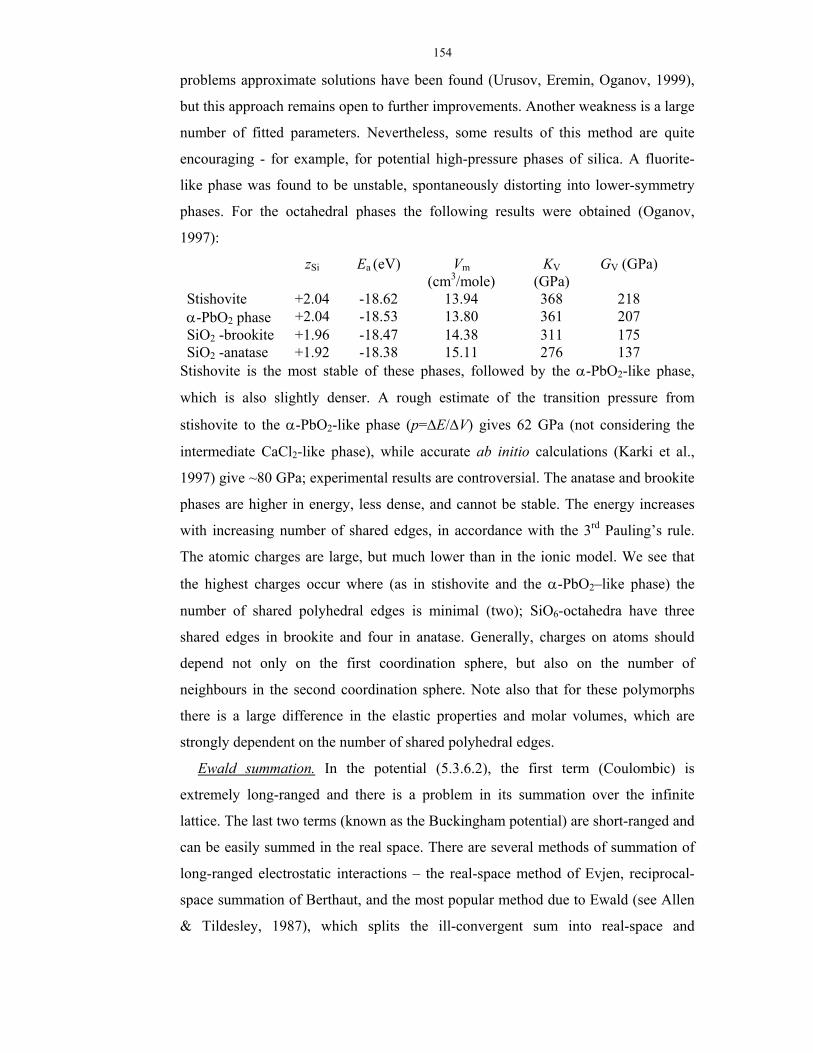
154
problems approximate solutions have been found (Urusov, Eremin, Oganov, 1999),
but this approach remains open to further improvements. Another weakness is a large
number of fitted parameters. Nevertheless, some results of this method are quite
encouraging - for example, for potential high-pressure phases of silica. A fluorite-
like phase was found to be unstable, spontaneously distorting into lower-symmetry
phases. For the octahedral phases the following results were obtained (Oganov,
1997):
zSi Ea (eV) Vm (cm3/mole)
KV (GPa)
GV (GPa)
Stishovite +2.04 -18.62 13.94 368 218 α-PbO2 phase +2.04 -18.53 13.80 361 207
SiO2 -brookite +1.96 -18.47 14.38 311 175 SiO2 -anatase +1.92 -18.38 15.11 276 137
Stishovite is the most stable of these phases, followed by the α-PbO2-like phase,
which is also slightly denser. A rough estimate of the transition pressure from
stishovite to the α-PbO2-like phase (p=∆E/∆V) gives 62 GPa (not considering the
intermediate CaCl2-like phase), while accurate ab initio calculations (Karki et al.,
1997) give ~80 GPa; experimental results are controversial. The anatase and brookite
phases are higher in energy, less dense, and cannot be stable. The energy increases
with increasing number of shared edges, in accordance with the 3rd Pauling’s rule.
The atomic charges are large, but much lower than in the ionic model. We see that
the highest charges occur where (as in stishovite and the α-PbO2–like phase) the
number of shared polyhedral edges is minimal (two); SiO6-octahedra have three
shared edges in brookite and four in anatase. Generally, charges on atoms should
depend not only on the first coordination sphere, but also on the number of
neighbours in the second coordination sphere. Note also that for these polymorphs
there is a large difference in the elastic properties and molar volumes, which are
strongly dependent on the number of shared polyhedral edges.
Ewald summation. In the potential (5.3.6.2), the first term (Coulombic) is
extremely long-ranged and there is a problem in its summation over the infinite
lattice. The last two terms (known as the Buckingham potential) are short-ranged and
can be easily summed in the real space. There are several methods of summation of
long-ranged electrostatic interactions – the real-space method of Evjen, reciprocal-
space summation of Berthaut, and the most popular method due to Ewald (see Allen
& Tildesley, 1987), which splits the ill-convergent sum into real-space and

155
reciprocal-space sums, whose convergence is good. Ewald summation is also an
ingredient of all periodic ab initio codes.
The derivation of the Ewald method follows two stages. First, we add to the
atomic point charges some atom-centred neutralising spherical charge distributions,
with the equal and opposite amount of charge. These distributions are usually takes
as Gaussians:
ρ = 2/3πκiz e
22rκ− , (5.3.6.10)
where κ is a parameter chosen to ensure good convergence. The neutralising
Gaussian distributions screen Coulombic interactions and make them short-ranged
and summable in the real space. Then, we add the same Gaussians, but now of the
same sign as the original charges. Their interactions can be summed in the reciprocal
space and transformed back into the real space. Spurious self-interaction, present in
this sum, must then be subtracted. Finally, the so-called surface term (non-vanishing
only in polar structures) is subtracted, giving the final result:
Ecoulombic = ∑ ∑∑ ∑= ≠
−
=
∞
=
π+
+
+N Nzz
Lzz
1i 0ij
4||
2
2
ji31j ij
ijj
0||i )]cos(exp
||41
|||)|(erfc
[21 2
2
K
K
nKr
Knrnr
κ
πκ
-
- ∑=π
Nz
1i
2i2/1
κ + 2
1iii3 ||
32 ∑
=
π Nz
Lr , (5.3.6.11)
where erfc(x) is the complementary error function: erfc(x) = dtex
t∫∞
−
π
2
2/12 . In the sum
(5.3.6.11) indices i and j denote atoms, n – lattice vectors, and K – reciprocal lattice
vectors.
Calculation of properties. With a given potential model and having a rough
starting structural model, it is easy to find the minimum energy structure – by using
the steepest descent, conjugate gradients, or damped molecular dynamics algorithms.
Near the equilibrium we can expand the energy as:
E = E0 + ½uTWuuu + uTWuee + ½eTWeee , (5.3.6.12)
where E0 is the equilibrium energy, u = (ux(1), uy(1), uz(1), ux(2), …, uz(n)) is a 1*3n
matrix of atomic positions, uT its transpose, and e is a 3*3 strain matrix. Wuu, Wue,
and Wee are the second derivative matrices defined as:
Wuu = )()( '
2
juiuE
αα ∂∂∂ ; Wue =
'
2
)( αα ejuE∂∂
∂ ; Wee = '
2
αα eeE∂∂
∂ (5.3.6.13)
156
At the equilibrium
u∂∂E = 0 = Wuuu + Wuee (5.3.6.14)
or
u = -W-1uuWuee (5.3.6.15)
With (5.3.6.12) our expansion (5.3.6.10) becomes
E = E0 + ½eT[Wεε - WeuW-1uuWue]e , (5.3.6.16)
from which we obtain the elastic constants tensor:
{cij} = V1 [Wεε - WeuW-1
uuWue] (5.3.6.17)
The last term in this equation represents the effect of internal strains on the elastic
constants. For more details and theory behind calculations of dielectric and
piezoelectric constants, see Catlow & Mackrodt (1982) and Dove (2002).
5.4. Lattice dynamics (LD).
Let us assume that ionic displacements are small enough for the interatomic
interactions to be harmonic, find the harmonic interatomic force constants as second
derivatives of the energy, and solve a system of Newtonian equations of motion
(derivation based on quantum mechanics leads to identical results). The solutions of
these equations are normal modes – independent harmonic oscillators involving
collective motions of atoms. For a crystal, we must take into account periodic
boundary conditions, which leads to 3n (n is the number of atoms in the unit cell)
equations of motion at each k-vector and 3n normal modes for each k-vector. There
is much resemblance in this procedure with the solution of one-electron equations of
quantum mechanics. For each normal mode, the solution gives the frequency and the
pattern of atomic displacements (from which one can determine the symmetry of the
vibration). Theory presented here is well described by Venkataraman et al. (1975)
and Dove (1993).
To obtain vibrational frequencies, at each k-point one should solve the following
determinantal equation:
det||D(k)- αβ2 ),( δνkω ijδ || = 0 , (5.4.1)
where D is the dynamical matrix, and ω2 are its eigenvalues. Indices α, β =1, 2, or 3
(x, y, z coordinates), and indices i and j denote different atoms within the unit cell.
Solving the eigenvalue problem (5.4.1) is equivalent to the diagonalisation of the

157
dynamical matrix, whose dimensions are 3n*3n. This leads to 3n solutions, denoted
by index ν.
Negative ω2 (i.e., imaginary ω) signify dynamical instability of the structure with
respect to a particular atomic motion, given by the mode eigenvectors, and indicate a
soft-mode driven phase transition. The soft-mode wave vector k determines the
direction and periodicity of the modulation imposed on the parent lattice at the phase
transition. The dynamical matrix D is defined as:
)(ikαβ kD = 2/1
ji )mm(1 ∑ −
lll )]0()((iexp[),0( ij
ijαβ rrkΦ , (5.4.2)
where mi and mj are masses of the i-th and j-th atoms, sum over l is the sum over all
unit cells (i.e. over the whole crystal), and ijαβΦ (0,l) are force constants between the
atom i in the reference cell (l=0) and atom j in the l-th cell, whose positions are
described by vectors ri(l) and rj(0). The force constant matrix ijαβΦ (l, l’) is defined
as:
ijαβΦ (l, l’) =
)'()( jβ
iα
2
luluE
∂∂∂ , (5.4.3)
where )(iα lu denotes a displacement of an i-th atom in the l-th unit cell along the α-
coordinate axis. The dynamical matrix can be thought of as a Fourier transform of
the force constant matrix times the 2/1ji )mm(
1 factor.
The solutions for the atomic displacements as a function of time are linear
combinations of plane wave-type functions and read as:
ui(l,t) = 2/1i )m(
1N
)]),()((iexp[),( i,
i tl ννν
kkrkUk
ω−∑ , (5.4.4)
where ),(i νkU is the amplitude vector, containing information on the direction and
amplitude of the displacement of all the i-th atoms under the influence of the ν-th
mode at the wavevector k. Usually, the time dependence and the amplitude are
grouped in the new quantity Q(k,ν) (called the normal coordinate), which leads to:
ui(l,t) = 2/1i )m(
1N
),()](iexp[),( i,
i ννν
kkrkek
Ql∑ , (5.4.5)
where the eigenvector ),(i νke , parallel to ),(i νkU , contains only the information
on the direction and symmetry of displacements. This vector is normalised:

158
∑i
2i |),(| νke = 1 (5.4.6)
This normalisation allows one to obtain atomic projections of the total phonon
density of states. For a longitudinal mode, ),(i νke is parallel to k; for a transverse
mode ),(i νke is perpendiculr to k. At a given k, the eigenvectors belonging to
different modes are orthogonal.
Normal coordinates provide an elegant way of expressing the kinetic energy of a
crystal:
<Ekin> = ∑ 2ων
νν,
2|),(|),(21
k
k kQ (5.4.7)
and the total harmonic energy:
<E> = <Ekin> + <Epot> = ∑ 2ων
νν,
2|),(|),(k
k kQ , (5.4.8)
from which the normal coordinate as a function of temperature is (Dove, 1993):
2|),(| νkQ = )1)),(exp(
121(
),(B
−+
ωTkk νων h
h
k (5.4.9)
In the classical limit we simply have 2|),(| νkQ = ),(2
B
νkωTk
.
To find the eigenvectors as well as eigenvalues, one must solve the following
equation:
ω2(k,ν)e(k,ν) = )(kD e(k,ν) (5.4.10)
All the above equations play the central role in lattice-dynamical calculations and
their interpretation. The most important application of LD is the calculation of
thermodynamic functions from the phonon density of states; basic theory and
equations were discussed in Chapter 3.
Calculation of the free energy enables the optimisation of the structure by
minimising the free energy within the quasiharmonic approximation. Usually, this is
done by computing the free energy derivatives numerically, within the so-called
ZSISA (Zero Static Internal Stress Approximation, in which only the unit cell
parameters are determined by the free energy minimisation, while all atomic
coordinates calculated by minimising the internal energy, rather than free energy)
and by assuming that the thermal pressure is isotropic (or, equivalently, that the
Grüneisen parameter is a simple scalar rather than a tensor).
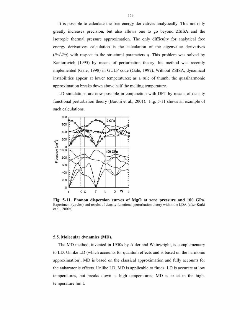
159
It is possible to calculate the free energy derivatives analytically. This not only
greatly increases precision, but also allows one to go beyond ZSISA and the
isotropic thermal pressure approximation. The only difficulty for analytical free
energy derivatives calculation is the calculation of the eigenvalue derivatives
(∂ω2/∂q) with respect to the structural parameters q. This problem was solved by
Kantorovich (1995) by means of perturbation theory; his method was recently
implemented (Gale, 1998) in GULP code (Gale, 1997). Without ZSISA, dynamical
instabilities appear at lower temperatures; as a rule of thumb, the quasiharmonic
approximation breaks down above half the melting temperature.
LD simulations are now possible in conjunction with DFT by means of density
functional perturbation theory (Baroni et al., 2001). Fig. 5-11 shows an example of
such calculations.
Fig. 5-11. Phonon dispersion curves of MgO at zero pressure and 100 GPa. Experiment (circles) and results of density functional perturbation theory within the LDA (after Karki et al., 2000a).
5.5. Molecular dynamics (MD).
The MD method, invented in 1950s by Alder and Wainwright, is complementary
to LD. Unlike LD (which accounts for quantum effects and is based on the harmonic
approximation), MD is based on the classical approximation and fully accounts for
the anharmonic effects. Unlike LD, MD is applicable to fluids. LD is accurate at low
temperatures, but breaks down at high temperatures; MD is exact in the high-
temperature limit.
160
In MD, we describe a classical system by the set of positions and velocities (ri(t),
vi(t)) of all particles. For a system of n atoms there are (3n-3) degrees of freedom,
and the classical kinetic energy is:
Ekin = ∑i
ii
2||m 2v =
2)33( BTkn − (5.5.1)
The initial kinetic energy (or temperature) is specified as an input, and the initial
velocities are assigned to the atoms randomly, according to the Maxwell distribution.
Having initial velocities thus specified and starting from the input configuration, the
system evolves with the atoms exploring trajectories, which are constructed by
solving Newtonian equations of motion. During this evolution, the atoms exchange
their kinetic energies, and the system equilibrates. Newton’s equations of motion are
conservative (i.e. there is no energy dissipation), the volume and the number of
particles are conserved as well, so here we are describing the microcanonical, or
NVE-, ensemble. Once equilibrated, the system explores all possible states having the
same energy E, and for some properties the expectation values can be computed as
the ensemble averages. One can introduce the instantaneous values of properties; for
example, the instantaneous values of the stress tensor41 are calculated as:
σij = -[ ijB δ
VTNk -
ij
pot1e
EV ∂
∂ ] , (5.5.2)
while for the instantaneous pressure we have the virial expression:
p = ijB δ
VTNk - ∑
iii3
1 rFV
(5.5.3)
Technical notes: 1. Trajectories can be calculated only by using a finite timestep
∆t (rather than infinitesimal dt). The most reliable algorithm for integrating the
equations of motion is the Verlet leapfrog algorithm:
ri(t+∆t) = 2ri(t) - ri(t-∆t) i
i tm
)(F (∆t)2 , (5.5.4)
where Fi(t) is the force acting on the i-th atom. The error in the positions is of the
order (∆t)4. ∆t must be sufficiently small (typically ~1 fs).
2. For simulating bulk materials, a large supercell should be used in conjunction with
periodic boundary conditions. The larger the system size, the more phonons are
41 Note the convention that stress tensor is positive when directed outwards, i.e. pressure and stress
have opposite signs. This is responsible for the minus sign in (5.5.2). Most simulation packages do
not take this minus sign into account.
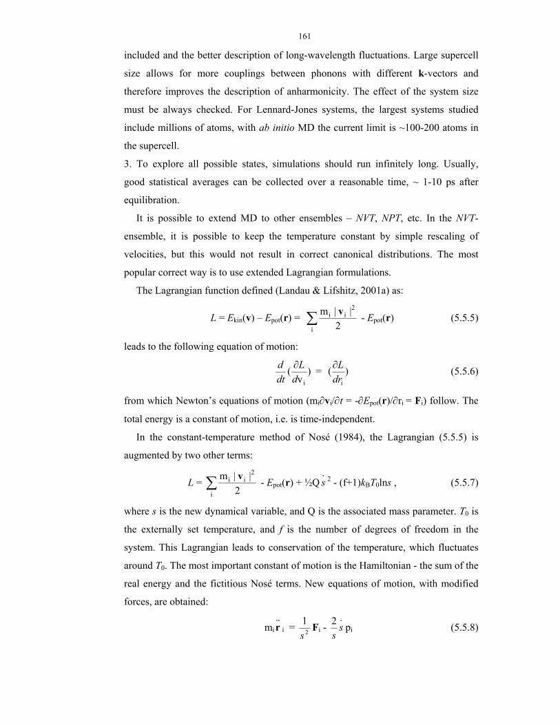
161
included and the better description of long-wavelength fluctuations. Large supercell
size allows for more couplings between phonons with different k-vectors and
therefore improves the description of anharmonicity. The effect of the system size
must be always checked. For Lennard-Jones systems, the largest systems studied
include millions of atoms, with ab initio MD the current limit is ~100-200 atoms in
the supercell.
3. To explore all possible states, simulations should run infinitely long. Usually,
good statistical averages can be collected over a reasonable time, ~ 1-10 ps after
equilibration.
It is possible to extend MD to other ensembles – NVT, NPT, etc. In the NVT-
ensemble, it is possible to keep the temperature constant by simple rescaling of
velocities, but this would not result in correct canonical distributions. The most
popular correct way is to use extended Lagrangian formulations.
The Lagrangian function defined (Landau & Lifshitz, 2001a) as:
L = Ekin(v) – Epot(r) = ∑i
2ii
2||m v - Epot(r) (5.5.5)
leads to the following equation of motion:
)v
(id
Ldtd ∂ = )(
idrL∂ (5.5.6)
from which Newton’s equations of motion (mi∂vi/∂t = -∂Epot(r)/∂ri = Fi) follow. The
total energy is a constant of motion, i.e. is time-independent.
In the constant-temperature method of Nosé (1984), the Lagrangian (5.5.5) is
augmented by two other terms:
L = ∑i
2ii
2||m v - Epot(r) + ½Q
.s 2 - (f+1)kBT0lns , (5.5.7)
where s is the new dynamical variable, and Q is the associated mass parameter. T0 is
the externally set temperature, and f is the number of degrees of freedom in the
system. This Lagrangian leads to conservation of the temperature, which fluctuates
around T0. The most important constant of motion is the Hamiltonian - the sum of the
real energy and the fictitious Nosé terms. New equations of motion, with modified
forces, are obtained:
mi..r i = 2
1s
Fi - .s
s2 pi (5.5.8)
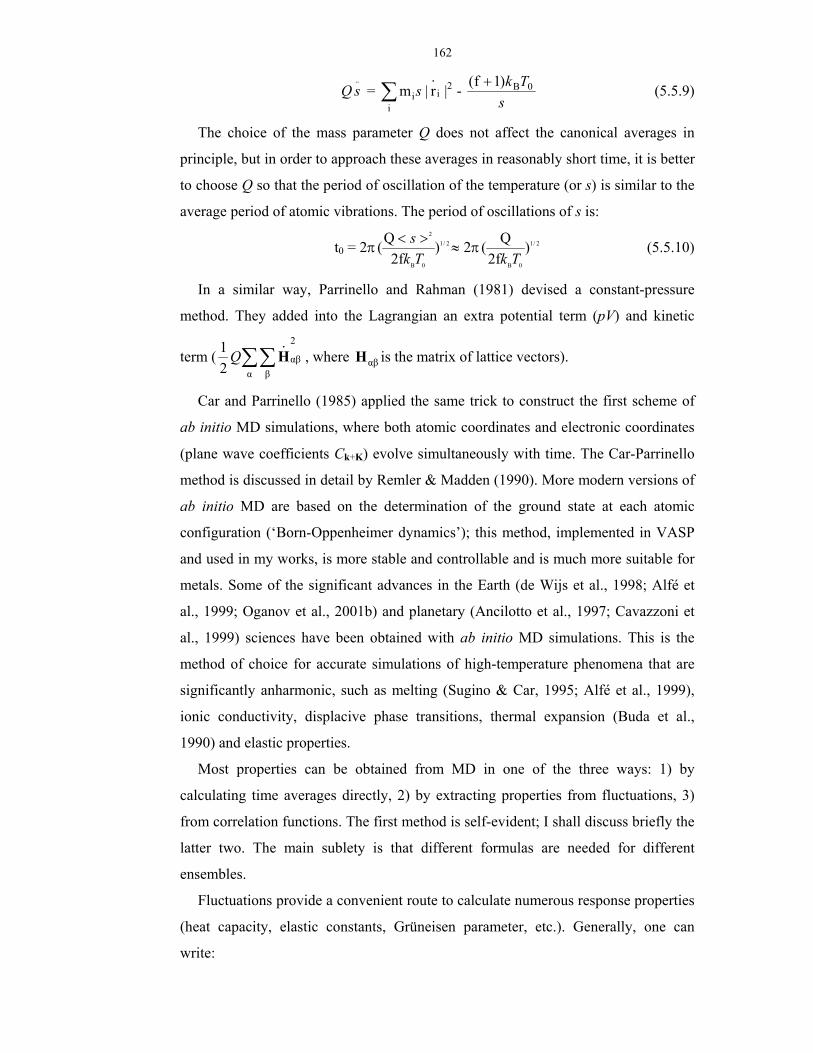
162
Q..
s = ∑i
2ii |r|m
.s -
sTk 0B)1f( + (5.5.9)
The choice of the mass parameter Q does not affect the canonical averages in
principle, but in order to approach these averages in reasonably short time, it is better
to choose Q so that the period of oscillation of the temperature (or s) is similar to the
average period of atomic vibrations. The period of oscillations of s is:
t0 = 2π 2/1
0B
2
)f2
Q(Tk
s ><≈ 2π 2/1
0B
)f2Q(
Tk (5.5.10)
In a similar way, Parrinello and Rahman (1981) devised a constant-pressure
method. They added into the Lagrangian an extra potential term (pV) and kinetic
term ( ∑∑α β
2
αβ21 .
HQ , where αβH is the matrix of lattice vectors).
Car and Parrinello (1985) applied the same trick to construct the first scheme of
ab initio MD simulations, where both atomic coordinates and electronic coordinates
(plane wave coefficients Ck+K) evolve simultaneously with time. The Car-Parrinello
method is discussed in detail by Remler & Madden (1990). More modern versions of
ab initio MD are based on the determination of the ground state at each atomic
configuration (‘Born-Oppenheimer dynamics’); this method, implemented in VASP
and used in my works, is more stable and controllable and is much more suitable for
metals. Some of the significant advances in the Earth (de Wijs et al., 1998; Alfé et
al., 1999; Oganov et al., 2001b) and planetary (Ancilotto et al., 1997; Cavazzoni et
al., 1999) sciences have been obtained with ab initio MD simulations. This is the
method of choice for accurate simulations of high-temperature phenomena that are
significantly anharmonic, such as melting (Sugino & Car, 1995; Alfé et al., 1999),
ionic conductivity, displacive phase transitions, thermal expansion (Buda et al.,
1990) and elastic properties.
Most properties can be obtained from MD in one of the three ways: 1) by
calculating time averages directly, 2) by extracting properties from fluctuations, 3)
from correlation functions. The first method is self-evident; I shall discuss briefly the
latter two. The main sublety is that different formulas are needed for different
ensembles.
Fluctuations provide a convenient route to calculate numerous response properties
(heat capacity, elastic constants, Grüneisen parameter, etc.). Generally, one can
write:
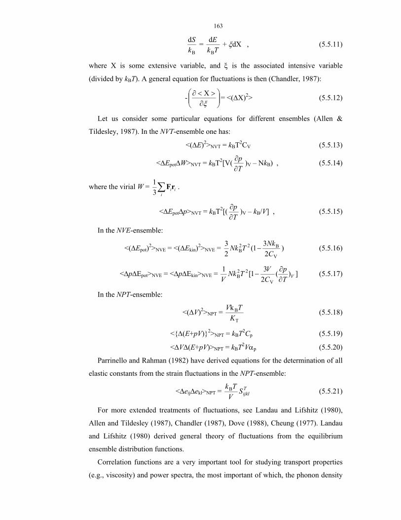
163
B
dkS =
TkE
B
d + ξdX , (5.5.11)
where X is some extensive variable, and ξ is the associated intensive variable
(divided by kBT). A general equation for fluctuations is then (Chandler, 1987):
-
∂
><∂ξX = <(∆X)2> (5.5.12)
Let us consider some particular equations for different ensembles (Allen &
Tildesley, 1987). In the NVT-ensemble one has:
<(∆E)2>NVT = kBT2CV (5.5.13)
<∆Epot∆W>NVT = kBT2[V(Tp
∂∂ )V – NkB) , (5.5.14)
where the virial W = ∑i
iirF31 .
<∆Epot∆p>NVT = kBT2[(Tp
∂∂ )V – kB/V] , (5.5.15)
In the NVE-ensemble:
<(∆Epot)2>NVE = <(∆Ekin)2>NVE = V
B22B 2
31(23
CNkTNk − ) (5.5.16)
<∆p∆Epot>NVE = <∆p∆Ekin>NVE = ])(231[1
V
22B VT
pCVTNk
V ∂∂
− (5.5.17)
In the NPT-ensemble:
<(∆V)2>NPT = T
BkK
TV (5.5.18)
<{∆(E+pV)}2>NPT = kBT2Cp (5.5.19)
<∆V∆(E+pV)>NPT = kBT2Vαp (5.5.20)
Parrinello and Rahman (1982) have derived equations for the determination of all
elastic constants from the strain fluctuations in the NPT-ensemble:
<∆eij∆ekl>NPT = TijklS
VTkB (5.5.21)
For more extended treatments of fluctuations, see Landau and Lifshitz (1980),
Allen and Tildesley (1987), Chandler (1987), Dove (1988), Cheung (1977). Landau
and Lifshitz (1980) derived general theory of fluctuations from the equilibrium
ensemble distribution functions.
Correlation functions are a very important tool for studying transport properties
(e.g., viscosity) and power spectra, the most important of which, the phonon density
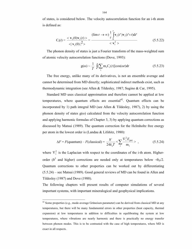
164
of states, is considered below. The velocity autocorrelation function for an i-th atom
is defined as:
Ci(t) = ><
><2|)0(|
)()0(
i
ii
v
vv t = ><
+∞→ ∫2i
0ii 'd)'()'(1)(lim
v
vvτ
ττ tttt
(5.5.22)
The phonon density of states is just a Fourier transform of the mass-weighted sum
of atomic velocity autocorrelation functions (Dove, 1993):
g(ω) ~ T1
∫ ∑i
ii d)ωcos()](m[ tttC (5.5.23)
The free energy, unlike many of its derivatives, is not an ensemble average and
cannot be determined from MD directly; sophisticated indirect methods exist, such as
thermodynamic integration (see Allen & Tildesley, 1987; Sugino & Car, 1995).
Standard MD uses classical approimation and therefore cannot be applied at low
temperatures, where quantum effects are essential42. Quantum effects can be
incorporated by 1) path integral MD (see Allen & Tildesley, 1987), 2) by using the
phonon density of states g(ω) calculated from the velocity autocorrelation function
and applying harmonic formulas of Chapter 3, 3) by applying quantum corrections as
discussed by Matsui (1989). The quantum correction for the Helmholtz free energy
per atom in the lowest order is (Landau & Lifshitz, 1980):
∆F = F(quantum) – F(classical) = TkB
2
24h <∑
∇
i
E
i
pot2i
m> , (5.5.24)
where 2i∇ is the Laplacian with respect to the coordinates of the i-th atom. Higher-
order (ħ3 and higher) corrections are needed only at temperatures below ~θD/2.
Quantum corrections to other properties can be worked out by differentiating
(5.5.24) – see Matsui (1989). Good general reviews of MD can be found in Allen and
Tildesley (1987) and Dove (1988).
The following chapters will present results of computer simulations of several
important systems, with important mineralogical and geophysical implications.
42 Some properties (e.g., mode-average Grüneisen parameter) can be derived from classical MD at any
temperatures, but there will be many fundamental errors in other properties (heat capacity, thermal
expansion) at low temperatures in addition to difficulties in equilibrating the system at low
temperatures, where vibrations are nearly harmonic and there is practically no energy transfer
between phonon modes. This is to be contrasted with the case of high temperatures, where MD is
exact in all respects.
165
Chapter 6. Antiordering in albite
(NaAlSi3O8).
This chapter will present a theoretical study of the anomalous antiordering in
albite recently found experimentally (Organova et al., 1999). The results are from
Oganov et al. (2001c), one of my earlier studies, actually performed in 1998. The
study is performed using crystal-chemical analysis supported by ionic shell model
calculations and preliminary Hartree-Fock calculations.
The antiordering phenomenon, i.e. preferential occupation of the Т2о positions by
the Al atoms, was found in the albite component of the two-phase feldspar from the
Pektusan volcano (Russian Far East). Ionic shell model calculations reproduce the
normal stability of the Т1o ordering, but show that the antiordered structure has a
lower energy at the experimental lattice parameters corresponding to the antiordered
sample. Simulations and crystal-chemical analysis conclude that antiordering can
take place as a result of a special strain (compression along c and/or stretching along
b). Such a deformation (stretching along b) does indeed occur in albite at the
coherent intergrowth boundaries (−601) with K-feldspar in the spinodal
decomposition structures from Pektusan volcano. K-feldspar lamellae experience an
opposite strain and show no change of the ordering scheme. Calculations also
indicate that the antiordered structure might become thermodynamically stable at
pressures of the order of a few GPa, corresponding to the deep lithosphere. The
predicted transition from the normal to the antiordered structure is isosymmetric.
Both ionic model calculations and preliminary Hartree-Fock simulations indicate a
correlation between the type of Al-Si ordering and the position of Na atoms in the
structure.
6.1. Introduction.
Crystal structures of alkali feldspars (MAlSi3O8) consist of the aluminosilicate
framework, whose cavities are occupied by large alkali atoms M = K and Na (Fig. 6-
1a). Si and Al are distributed over 2 crystallographically independent positions (Т1
and Т2) in the monoclinic disordered structure (C2/m) or over 4 positions (T1o , T1m,

166
T2o, and T2) in the ordered triclinic C−
1 structure. There are 5 oxygen positions (OA1,
OA2, OB, OC, and OD) in the monoclinic and 8 in the triclinic structure.
a b
Fig. 6-1. Feldspar structure. (a) General view. Yellow spheres – alkali atoms in the cavities of the tetrahedral framework. Blue and red – T1- and T2-tetrahedra, respectively. (b) Detailed scheme of the framework. Spheres denote centres of the aluminosilicate tetrahedra. Large spheres: Т1-, small spheres: Т2-tetrahedra. Tetrahedral chains running along the b axis (1 period = 4T2+2T1) and c axis (1 period = 2T1+1T2) are highlighted.
All structural studies have shown that Al preferentially occupies the T1 position in
monoclinic (T1o in triclinic) alkali feldpars. At low temperatures, alkali feldspar solid
solutions exsolve into K- and Na-components, but some limited mutual solubility is
always present.
Recently, an anomalous sample of two-phase feldspar from the Russian Far East
was found and studied (Organova et al., 1999). The sample was found by V.V.
Nasedkin near the Pektusan volcano. The sample crystallised at the depth of 5-6 km
at temperatures of ~1173-1273 K and pressures of ~0.3 GPa. This material was later
brought to the surface as a result of an explosive eruption. The sample was studied
by single crystal structural refinement, electron microprobe analysis, and high-
resolution electron microscopy. The latter method showed that the sample is a
product of spinodal decomposition with alternating lamellae of K- and Na-
components with the intergrowth boundary (−601). The average thickness of the K-
lamellae is 40 Å; Na-lamellae are 120 Å thick. Structural refinements showed two
anomalies. First, both phases had a monoclinic shape of the unit cell. Second, Al was
found to concentrate in the T2о, rather than T1о, positions. Results of structural
refinements of both phases for the space group C−
1 are given in Table 6-1.
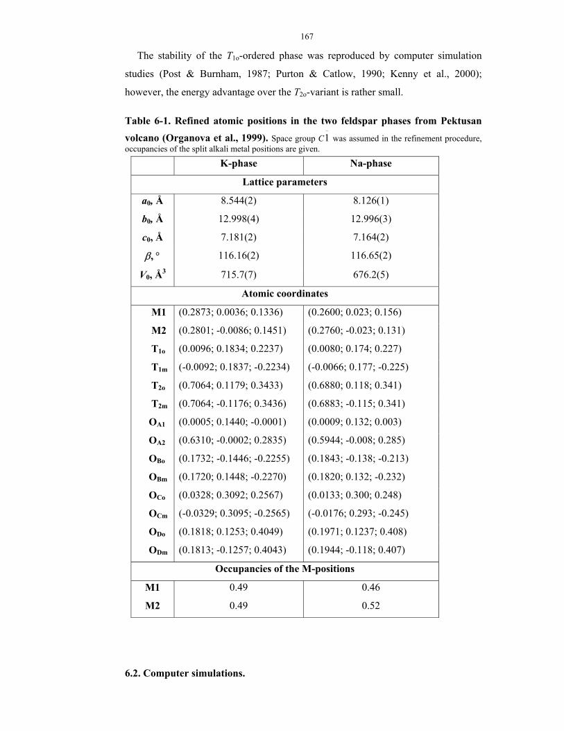
167
The stability of the T1о-ordered phase was reproduced by computer simulation
studies (Post & Burnham, 1987; Purton & Catlow, 1990; Kenny et al., 2000);
however, the energy advantage over the T2о-variant is rather small.
Table 6-1. Refined atomic positions in the two feldspar phases from Pektusan volcano (Organova et al., 1999). Space group C
−
1 was assumed in the refinement procedure, occupancies of the split alkali metal positions are given.
K-phase Na-phase
Lattice parameters
a0, Å 8.544(2) 8.126(1)
b0, Å 12.998(4) 12.996(3)
c0, Å 7.181(2) 7.164(2)
β, ° 116.16(2) 116.65(2)
V0, Å3 715.7(7) 676.2(5)
Atomic coordinates
M1 (0.2873; 0.0036; 0.1336) (0.2600; 0.023; 0.156)
М2 (0.2801; -0.0086; 0.1451) (0.2760; -0.023; 0.131)
Т1o (0.0096; 0.1834; 0.2237) (0.0080; 0.174; 0.227)
Т1m (-0.0092; 0.1837; -0.2234) (-0.0066; 0.177; -0.225)
Т2o (0.7064; 0.1179; 0.3433) (0.6880; 0.118; 0.341)
Т2m (0.7064; -0.1176; 0.3436) (0.6883; -0.115; 0.341)
ОА1 (0.0005; 0.1440; -0.0001) (0.0009; 0.132; 0.003)
ОА2 (0.6310; -0.0002; 0.2835) (0.5944; -0.008; 0.285)
ОВo (0.1732; -0.1446; -0.2255) (0.1843; -0.138; -0.213)
ОВm (0.1720; 0.1448; -0.2270) (0.1820; 0.132; -0.232)
ОСo (0.0328; 0.3092; 0.2567) (0.0133; 0.300; 0.248)
ОСm (-0.0329; 0.3095; -0.2565) (-0.0176; 0.293; -0.245)
ОDo (0.1818; 0.1253; 0.4049) (0.1971; 0.1237; 0.408)
ODm (0.1813; -0.1257; 0.4043) (0.1944; -0.118; 0.407)
Occupancies of the M-positions
M1 0.49 0.46
M2 0.49 0.52
6.2. Computer simulations.

168
It is well known (Burnham, 1990) that the ionic shell model is very successful at
describing structures of silicates. This model also successfully reproduces the
elasticity of crystal structures and their components – bonds and polyhedra. This is
particularly important in the present case, where the unit cells of feldspar minerals
are deformed (unit cell of albite is expanded by 1.51%, that of K-feldspar –
compressed by 0.95%) because of the fine intergrowth along coherent phase
boundaries.
The simplest setting of the problem includes the consideration of only the two
limiting cases: 1) fully ordered with Al in Т1o (MAlT1oSiT1m (SiT2)2O8), and 2)
antiordered (MAlT2oSiT2m(SiT1)2O8) phases. Calculations were performed using the
METAPOCS code (Parker, 1983) adapted to IBM PC (Urusov et al., 1994). I also
performed calculations on the fully disordered phases (high albite and sanidine)
using the virtual crystal formulation of Winkler et al. (1991).
The potential model used in the calculations included pairwise interactions
(5.3.6.2), shell model (5.3.6.6), and three-body angle-bending potentials (5.3.6.8).
There exist good sets of potential parameters for Si-O, Al-O, O-Si-O, O-O
interactions and for the shell model of O2-; I used parameters from (Catlow, 1977;
James, 1979; Sanders et al., 1984). On the contrary, there are no well-established
potential parameters for K-O and Na-O interactions. Therefore, it is preferable to use
several models for these interactions and trust only those results, which are similar in
different models. I used three different potentials for the Na-O and K-O interactions:
potential calculated by the modified electron gas method (MEG) (Post & Burnham,
1986), empirical potential (EP), obtained by simultaneous fitting to a large number of
structures (Bush et al., 1994), and my own potential (AP), which was derived a
priori, using equation (5.3.6.3) and tables of ionic radii. Potential parameters are
given in Table 6-2; AP- and MEG-potentials for Na-O are compared in Fig. 6-2. All
potentials lead to reasonable predictions of the structures and properties; the best
structural predictions are given by the MEG model. For high-symmetry solutions
Born stability criteria were checked using the calculated elastic constants. These
indicated a triclinic distortion of the disordered albite structure (see below).

169
Fig. 6-2. Na-O potential: MEG and AP models.
Table 6-2. Parameters of the ionic shell model for (Na,K)AlSi3O8. ( ZSi =+4.00 ; ZAl =+3.00; ZO =-2.00).
Pair potentials
Interaction bij, eV ρij, Å cij, eV* Å6
O-O 22764.3 0.1490 27.88
AlIV-O 1460.3 0.29912 0
SiIV-O 1283.9 0.3205 10.66
Na-O (MEG) 5836.814 0.2387 0
Na-O (EP) 1271.504 0.3000 0
Na-O (AP) 864.0 0.3110 0
K-O (MEG) 65269.710 0.2134 0
K-O (EP) 3587.500 0.3000 0
K-O (AP) 1789.3 0.3200 0
Shell parameters (only for O2-)
ks (O)=74.9204 eV*Å-2. q(shell) = -2.84819. Q(core) = +0.84819
Three-body potentials (only for tetrahedral coordination; ϕ0 = 109.47°)
kb (O-Al-O)= kb (O-Si-O)=2.09724 eV/rad2

170
6.3. Results.
Simulations correctly reproduce crystal structures of feldspars; some results are
given in Tables 6-3 to 6-6 (compare with experimantal data from Table 6-1). Space
group C2/m is correctly given for the fully disordered K-feldspar (sanidine). For high
albite, in accordance with experiment, the C2/m solution is mechanically unstable
(condition C44>0 is violated) in the MEG- and AP-models, and the space group is
lowered to C1−
. This symmetry lowering is accompanied by the collapse of the
aluminosilicate framework around the Na+, which is too small to support large
cavities of the undistorted framework. EP-potential, overestimating the Na-O
repulsion and, as a consequence, the effective size of Na+ ions, does not give this
symmetry lowering. In the case of sanidine with a larger K+, the monoclinic structure
is stable in all the three models.
Let us first consider albite. All the three models show that the T2o-structure has a
higher energy and a higher density than the T1o-structure and therefore should
become thermodynamically stable at high pressures; estimates based on ptr=∆E/∆V
are 0.3 GPa, 5.0 GPa, and 11 GPa for the MEG-, AP-, and EP-models, respectively.
Therefore, it is possible that this transition takes place in the deep parts of the
lithosphere, at pressures of a few GPa. Since both ordering schemes (T1o and T2o)
result in the same symmetry (C1−
), the transition should be isosymmetric; it must be
first-order, but will become fully continuous above the critical temperature (which in
this case is the temperature of Al-Si disordering).
All the three models show the following trends for the lattice parameters: increase
of a0 (by 0.7%) and c0 (by 0.8%) in the sequence T2o→disordered→T1o and increase
of b0 by 1% in the opposite sequence T1o→disordered→T2o. The clear dependence of
the b0 and c0 parameters on the degree of ordering is well known from experiment
and was used (Stewart & Wright, 1974) as a basis of an X-ray diffraction method of
determination of the degree of ordering of feldspars.
Table 6-3 shows a significant difference in the coordinates of the Na atom in the
T1o- and T2o-structures (the difference in the z coordinate reaches 0.052). This
corresponds well to the experimentally observed ‘splitting’ of the Na position in
partially ordered albites. The splitting of other atomic positions is much smaller.
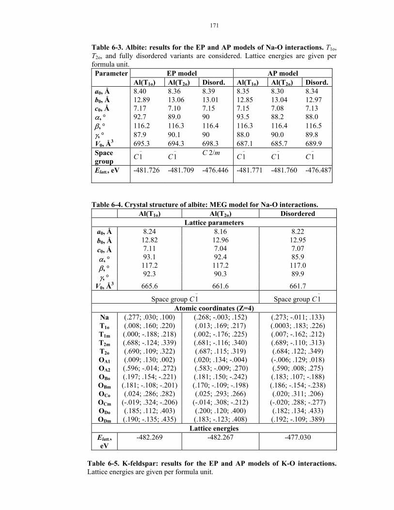
171
Table 6-3. Albite: results for the EP and AP models of Na-O interactions. T1o, T2o, and fully disordered variants are considered. Lattice energies are given per formula unit. Parameter EP model AP model Al(T1o) Al(T2o) Disord. Al(T1o) Al(T2o) Disord. a0, Å 8.40 8.36 8.39 8.35 8.30 8.34 b0, Å 12.89 13.06 13.01 12.85 13.04 12.97 c0, Å 7.17 7.10 7.15 7.15 7.08 7.13 α, ° 92.7 89.0 90 93.5 88.2 88.0 β, ° 116.2 116.3 116.4 116.3 116.4 116.5 γ, ° 87.9 90.1 90 88.0 90.0 89.8 V0, Å3 695.3 694.3 698.3 687.1 685.7 689.9 Space group C1
−
C1−
C 2/m C1−
C1−
C1−
Elatt., eV -481.726
-481.709
-476.446
-481.771
-481.760
-476.487
Table 6-4. Crystal structure of albite: MEG model for Na-O interactions. Al(T1o) Al(T2o) Disordered
Lattice parameters a0, Å b0, Å c0, Å α, ° β, ° γ, °
8.24 12.82 7.11 93.1 117.2 92.3
8.16 12.96 7.04 92.4 117.2 90.3
8.22 12.95 7.07 85.9 117.0 89.9
V0, Å3 665.6 661.6 661.7
Space group C1−
Space group C1−
Atomic coordinates (Z=4)
Na (.277; .030; .100) (.268; -.003; .152) (.273; -.011; .133) T1o (.008; .160; .220) (.013; .169; .217) (.0003; .183; .226) T1m (.000; -.188; .218) (.002; -.176; .225) (.007; -.162; .212) T2m (.688; -.124; .339) (.681; -.116; .340) (.689; -.110; .313) T2o (.690; .109; .322) (.687; .115; .319) (.684; .122; .349) OA1 (.009; .130; .002) (.020; .134; -.004) (-.006; .129; .018) OA2 (.596; -.014; .272) (.583; -.009; .270) (.590; .008; .275) OBo (.197; .154; -.221) (.181; .150; -.242) (.183; .107; -.188) OBm (.181; -.108; -.201) (.170; -.109; -.198) (.186; -.154; -.238) OCo (.024; .286; .282) (.025; .293; .266) (.020; .311; .206) OCm (-.019; .324; -.206) (-.014; .308; -.212) (-.020; .288; -.277) ODo (.185; .112; .403) (.200; .120; .400) (.182; .134; .433) ODm (.190; -.135; .435) (.183; -.123; .408) (.192; -.109; .389)
Lattice energies Elatt., eV
-482.269
-482.267
-477.030
Table 6-5. K-feldspar: results for the EP and AP models of K-O interactions. Lattice energies are given per formula unit.

172
Parameter EP model AP model Al(T1o) Al(T2o) Disord. Al(T1o) Al(T2o) Disord. a0, Å 9.00 8.96 8.98 8.94 8.91 8.92 b0, Å 12.92 13.11 13.03 12.93 13.12 13.04 c0, Å 7.26 7.18 7.23 7.25 7.17 7.22 α, ° 90.6 89.9 90 90.7 89.8 90 β, ° 115.9 115.8 115.8 115.9 115.8 115.8 γ, ° 88.1 90.4 90 88.0 90.3 90 V0, Å3 758.0 759.4 760.7 753.1 754.3 755.7 Space group C1
−
C1−
C 2/m C1−
C1−
C 2/m
Elatt., eV -480.932 -480.926 -475.675 -480.953 -480.942 -475.691 Table 6-6. Crystal structure of K-feldspar: MEG model for K-O interactions.
Al(T1o) Al(T2o) Disordered Lattice parameters
a0, Å b0, Å c0, Å α, ° β, ° γ, °
8.59 12.93 7.18 90.7 116.1 87.8
8.57 3.09 7.11 89.8 116.1 90.5
8.58 13.03 7.15 90
116.1 90
V0, Å3 715.53 716.66 718.35 Atomic coordinates
K (.282; -.008; .142) (.283; -.002; .139) (.282; 0; .140) T1o (.008; .186; .215) (.013; .181; .224) (.008; .183; .222) T1m (.007; -.179; .231) (.006; -.185; .221) (.008; -.183; .222) T2m (.705; -.116; .350) (.708; -.118; .340) (.709; -.118; .342) T2o (.713; .119; .337) (.709; .117; .342) (.709; .118; .342) OA1 (.002; .142; -.018) (.016; .145; .008) (0; .143; 0) OA2 (.636; .005; .284) (.632; -.007; .281) (.633; 0; .283) OBo (.172; .145; -.236) (.172; .146; -.226) (.172; .145; -.223) OBm (.179; -.145; -.214) (.163; -.145; -.217) (.172; -.145; -.223) OCo (.036; .318; .252) (.044; .304; .260) (.037; .308; .256) OCm (-.044; .304; -.269) (-.027; .306; -.246) (-.037; .308; -.256) ODo (.189; .124; .406) (.180; .127; .408) (.178; .126; .405) ODm (.170; -.124; .414) (.171; -.127; .390) (.178; -.126; .405)
Lattice energies Elatt., eV -481.744 -481.714 -476.467
Results for K-feldspar (Tables 6-5 and 6-6) show that T1o-structure is again the
most stable one. However, all the three models indicate that the T1o-structure also has
the highest density and will be stable also at high pressures, unlike albite. Parameter
a0 is practically independent of the degree of ordering (its changes are within 0.03
Å). Like for albite, all the three models show an increase of b0 by 1.4% in the
sequence T1o→disordered→T2o and decrease of c0 by 1.1% in the same sequence.
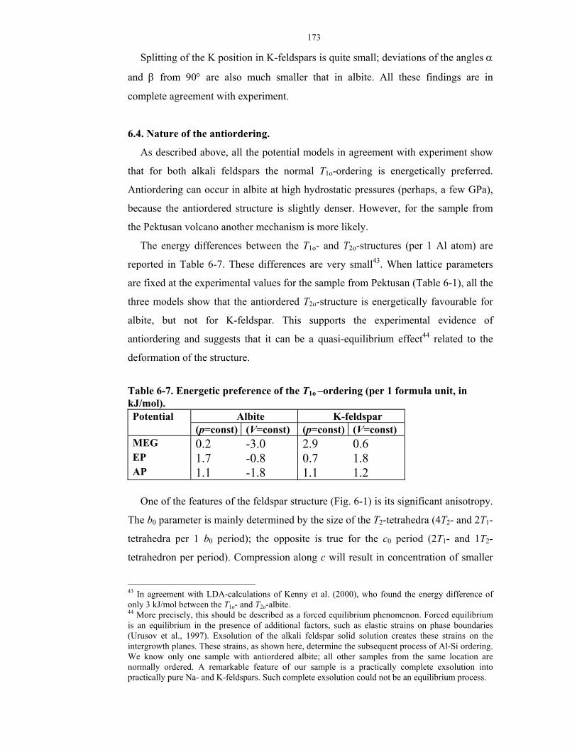
173
Splitting of the K position in K-feldspars is quite small; deviations of the angles α
and β from 90° are also much smaller that in albite. All these findings are in
complete agreement with experiment.
6.4. Nature of the antiordering.
As described above, all the potential models in agreement with experiment show
that for both alkali feldspars the normal T1о-ordering is energetically preferred.
Antiordering can occur in albite at high hydrostatic pressures (perhaps, a few GPa),
because the antiordered structure is slightly denser. However, for the sample from
the Pektusan volcano another mechanism is more likely.
The energy differences between the T1o- and T2o-structures (per 1 Al atom) are
reported in Table 6-7. These differences are very small43. When lattice parameters
are fixed at the experimental values for the sample from Pektusan (Table 6-1), all the
three models show that the antiordered T2о-structure is energetically favourable for
albite, but not for K-feldspar. This supports the experimental evidence of
antiordering and suggests that it can be a quasi-equilibrium effect44 related to the
deformation of the structure.
Table 6-7. Energetic preference of the T1o –ordering (per 1 formula unit, in kJ/mol).
Albite K-feldspar Potential (p=const) (V=const) (p=const) (V=const)
MEG 0.2 -3.0 2.9 0.6 EP 1.7 -0.8 0.7 1.8 AP 1.1 -1.8 1.1 1.2
One of the features of the feldspar structure (Fig. 6-1) is its significant anisotropy.
The b0 parameter is mainly determined by the size of the T2-tetrahedra (4T2- and 2T1-
tetrahedra per 1 b0 period); the opposite is true for the c0 period (2T1- and 1T2-
tetrahedron per period). Compression along c will result in concentration of smaller
43 In agreement with LDA-calculations of Kenny et al. (2000), who found the energy difference of only 3 kJ/mol between the T1o- and T2o-albite. 44 More precisely, this should be described as a forced equilibrium phenomenon. Forced equilibrium is an equilibrium in the presence of additional factors, such as elastic strains on phase boundaries (Urusov et al., 1997). Exsolution of the alkali feldspar solid solution creates these strains on the intergrowth planes. These strains, as shown here, determine the subsequent process of Al-Si ordering. We know only one sample with antiordered albite; all other samples from the same location are normally ordered. A remarkable feature of our sample is a practically complete exsolution into practically pure Na- and K-feldspars. Such complete exsolution could not be an equilibrium process.
174
Si atoms in T1 positions and outflow of Al into T2, with antiordering as the end result
(if compression is large enough). Analogously, stretching along b will result in
antiordering. The opposite result (i.e. enhancement of the tendency to normal
ordering) would be created by compression along b and/or stretcing along c axis.
There must be good matching of the lattice parameters of the two phases at the
coherent intergrowth boundaries. As a result, the unit cell of albite is expanded, and
that of K-feldspar – compressed relative to unstrained samples. In our sample, the
largest stretching is along b and much smaller – along c. This is consistent with the
fact that the intergrowth plane is (−601); b axis lies in this plane, explaining why the
largest deformation is along this axis. Stretching along b axis should lead to
antiordering; this was observed in the sample from the Pektusan volcano. In K-
feldspar the deformation is opposite, and there is no change in the ordering scheme.
6.5. Hartree-Fock calculations: correlation of Na position and Al-Si ordering in
albite.
Some preliminary Hartree-Fock calculations have been performed with the
CRYSTAL95 code (Dovesi et al., 1996). In these calculations, performed on a
Pentium II PC, I used a minimal basis set STO-3G and fixed experimental geometry
from Table 6-1, with all Al in the T2о positions and all Na either in the M1 (column
‘Na1’ in Table 6-8) or in the M2 (column ‘Na2’) positions. 2*2*2-mesh (4 unique
points), used for the Brillouin zone sampling, leads to a very good convergence of all
calculated properties. Recommended (Dovesi et al., 1996) integration tolerances
were used for bielectronic integrals: ITOL1, ITOL2, ITOL3, ITOL4 and ITOL5 were
equal to 10-6, 10-6, 10-6, 10-6 and 10-12, respectively.
Table 6-8 shows the Mulliken charges of atoms and total energies of the ‘Na1’
and ‘Na2’ structures. One can see that with T2о–ordering Na atoms strongly prefer
the M2 position (by 0.20 eV/(atom Na) or 19.4 kJ/mol). This is in agreement with the
ionic shell model, which showed (Table 6-4) that the position of the Na atom
depends on the type of ordering. Indeed, in our antiordered sample Na occupies M2
position more (Table 6-4). The ratio of the site occupancies Na1/Na2 should be
directly related to the type and degree of ordering.
Table 6-8. Mulliken charges and total energy of albite from Hartree-Fock calculations (STO-3G basis).
Position Na1 Na2
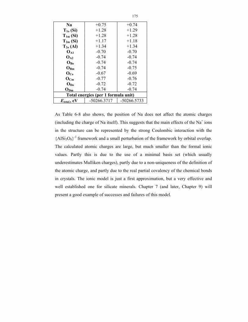
175
Na +0.75 +0.74 T1o (Si) +1.28 +1.29 T1m (Si) +1.28 +1.28 T2m (Si) +1.17 +1.18 T2o (Al) +1.34 +1.34
OA1 -0.70 -0.70 OA2 -0.74 -0.74 OBo -0.74 -0.74 OBm -0.74 -0.75 OCo -0.67 -0.69 OCm -0.77 -0.76 ODo -0.72 -0.72 ODm -0.74 -0.74 Total energies (per 1 formula unit)
Etotal., eV -50266.3717 -50266.5733
As Table 6-8 also shows, the position of Na does not affect the atomic charges
(including the charge of Na itself). This suggests that the main effects of the Na+ ions
in the structure can be represented by the strong Coulombic interaction with the
{AlSi3O8}-1 framework and a small perturbation of the framework by orbital overlap.
The calculated atomic charges are large, but much smaller than the formal ionic
values. Partly this is due to the use of a minimal basis set (which usually
underestimates Mulliken charges), partly due to a non-uniqueness of the definition of
the atomic charge, and partly due to the real partial covalency of the chemical bonds
in crystals. The ionic model is just a first approximation, but a very effective and
well established one for silicate minerals. Chapter 7 (and later, Chapter 9) will
present a good example of successes and failures of this model.

176
Chapter 7. Ionic modelling of Al2SiO5
polymorphs.
This chapter is rather introductory – it presents an overview of the mineralogy of
the Al2SiO5 polymorphs and their study with simple semiclassical simulations based
on the ionic shell model. This will be followed by the application of much more
powerful techniques to the same minerals in Chapters 8 and 9. The results presented
in this chapter are from my MSc thesis (Oganov, 1997) and an early paper (Urusov et
al., 1998); only a few selected results from these works are presented here. These
results were obtained using the METAPOCS code (Parker, 1983) in a version
adapted to IBM PC (Urusov et al., 1994). Note that different results are sometimes
obtained with the more modern GULP code, but the difference is insignificant.
7.1. Introduction.
Crystal structures of the Al2SiO5 polymorphs (kyanite, andlausite, sillimanite)
were first solved in 1928-1929 and refined many times since, by neutron and,
mainly, X-ray diffraction. High-temperature (Winter & Ghose, 1979) and high-
pressure (Ralph et al., 1984; Yang et al., 1997a,b; Comodi et al., 1997) studies have
been performed. A comprehensive review (Kerrick, 1990) exists on these minerals.
Kyanite is triclinic (P1−
), andalusite and sillimanite are orthorhombic (Pnnm and
Pbnm, respectively). Their structures are depicted in Fig.4-3. In these structures, Si is
tetrahedrally coordinate. In all these structures, half of the Al positions are
octahedrally coordinated, whereas the other half is either tetrahedrally (sillimanite),
again octahedrally (kyanite) or fivefold coordinate (andalusite). It is possible to
consider sillimanite as a band aluminosilicate with the band polyanions [AlSiO5]3-
running along the c axis. All the three minerals have chains of edge-sharing Al-
octahedra along the c axis. These chains make andalusite and sillimanite highly
anisotropic minerals. Anisotropy is pronounced in their thermal expansion (Winter,
Ghose, 1979), linear compressibilities and elastic constants (Vaughan & Weidner,
1978). The dense structure of kyanite is based on the cubic close packing of the
oxygens; electron microscopy revealed a polytype with a 4-layer packing (Grobety
& Veblen, 1995).

177
Only kyanite satisfies the II Pauling’s rule (local charge balance), which explains
why kyanite is the lowest-energy phase. On the other hand, the kyanite structure has
the largest number of shared polyhedral edges, which should destabilise it by the III
Pauling’s rule. In fact, the least stable structure (sillimanite) has the lowest number
of shared polyhedral edges. However, that the energy differences between these
phases are very small.
Sillimanite is structurally close to incommensurately modulated mullite
(~3Al2O3*2SiO2), which is formed as a product of incongruent melting of
sillimanite. Kyanite is structurally related to staurolite Fe2Al9Si4O22(OH)2, whose
structure contains kyanite layers alternating with layers of the composition
AlOOH*2FeO; this explains the frequent intergrowth of the two minerals.
Vaughan and Weidner (1978) have measured the elastic constants of andalusite
and sillimanite and related them to the crystal structures. Combination of accurate
IR- and Raman spectra with model forcefields has lead to first lattice-dynamical
models and phonon spectra of andalusite (Iishi et al., 1979; Salje & Werneke,
1982a,b) and sillimanite (Salje & Werneke, 1982a,b). Winkler and Buehrer (1990)
and Rao et al. (1999) have successfully used semiclassical simulations to study the
lattice dynamics of the Al2SiO5 polymorphs.
All Al2SiO5 polymorphs melt incongruently into mullite and SiO2 melt: sillimanite
at 1545°C, andalusite at 1400°С, and kyanite at 1510°C; metastable congruent
melting of sillimanite occurs at 1816°С. Due to incongruent melting, these minerals
are never found in magmatic rocks, but are typical metamorphic minerals. Their
phase diagram, very important in the context of metamorphic petrology, has attracted
much attention over the last 50 years (see, e.g., Zen, 1969; Kerrick, 1990;
Hemingway et al., 1991; Olbricht et al., 1994).
For a long time, the determination of the phase diagram of Al2SiO5 posed a
problem, due to the very small energy differences between the polymorphs. Now the
problem seems to have been solved (Olbricht et al., 1994). It is interesting to note
that transition metal impurities can significantly alter the stability fields of these
minerals (Cr enhances the stability of kyanite, Mn stabilises andalusite). Salje (1986)
experimentally demonstrated that fibrolite (fine-grained highly defective sillimanite)
has a significantly higher heat capacity than sillimanite, and the grain size affects the
phase diagram. Combination of neutron diffraction and NMR (Stebbins et al., 1993)
showed that fibrolite has a complete Al-Si order, but there is a significant disorder in
178
the relative location of the fully ordered [AlSiO5] bands along the c axis. Full Al-Si
disorder in sillimanite is expected to occur at ~1700-1800 °C (Holland & Carpenter,
1986), well above the incongruent melting temperature. Thermodynamic functions
have been measured many times; they have been tabulated by Robie and Hemingway
(1995).
7.2. Mineralogy of Al in the lower mantle.
Although Al is expected to be one of the most abundant elements in the Earth’s
lower mantle (Table 2-1), not much is known about its mineralogy in that region.
The mineralogy of Al is of particular interest, since if Al does not form a separate
phase, it must be predominantly contained in (Mg,Fe)SiO3-perovskite. It has been
shown that if this is the case, it would radically change Fe/Mg-partitioning and phase
equilibria (Wood and Rubie, 1996) between perovskite and magnesiowüstite,
leading to significant enrichment of perovskite in Fe (especially in the form of Fe3+)
(McCammon, 1997), and that would change dramatically many physical and
chemical properties (e.g. electrical conductivity, thermodynamic, rheological and
diffusional properties) of perovskite. These changes could strongly affect the current
geophysical and geochemical models of the mantle.
Based on the high-pressure experiments on pyrolitic material at 1800-1900 K and
23-28 GPa, Irifune (1994) has concluded that MgSiO3-perovskite should be the main
host of Al in the lower mantle, being able to accommodate all Al present in the lower
mantle. This closely corresponds to results of Liu (1977), who showed that up to 25
mol.% of Al2O3 can be present in MgSiO3-based perovskite solid solution. However,
many other experimental studies (Madon et al., 1989; Irifune et al., 1991; Ahmed-
Zaid & Madon, 1991, 1995) reveal high-pressure aluminous phases that have been
proposed to be the main hosts of Al in the lower mantle. In the earlier work, Irifune
et al. (1991) proposed a high-pressure form of MgAl2O4 with the CaFe2O4 structure
as the main Al-phase in the lower mantle; recently, Funamori et al. (1998)
synthesised an even denser phase with the CaTi2O4 structure, stable at higher
pressures. Another candidate is a high-pressure modification of (Ca,Mg)Al2Si2O8
with a hollandite-like structure (Madon et al. 1989).
Most attention has been paid to a possible high-pressure phase of Al2SiO5. Birle
and Ehlers (1969) have studied a high-pressure phase transition of Al2GeO5 at 3.5
GPa and concluded that such a transition could occur in Al2SiO5 at 15 GPa. Powder
179
diffraction data on this phase did not allow the authors to identify the crystal
structure of this new phase, although many of the diffraction lines can be indexed
assuming the pseudobrookite structure (Oganov, 1997). At the same time Ringwood
and Reid (1969) showed that Al2GeO5 decomposes to Al2O3 + GeO2 at high
pressures and Liu (1974) found that a similar decomposition of kyanite into
corundum (Al2O3) + stishovite (SiO2) at pressures 14-16 GPa and temperatures
1300-1700 K.
However, in the more recent experiments of Ahmed-Zaid and Madon (1991,
1995), a high-pressure form of Al2SiO5 with the V3O5-type structure was found at
40-70 GPa and 2500 K. Lattice parameters were measured for this phase and, on the
basis of these values and the composition, it was found found that at the atmospheric
pressure the V3O5-type phase of Al2SiO5 is 4.5% denser than the isochemical
mixture of corundum and stishovite. The fact that this phase was formed as a high-
pressure product in all studied samples of kyanite (Al2SiO5), anorthite (CaAl2Si2O8),
grossular (Ca3Al2Si3O12) and pyrope (Mg3Al2Si3O12), supported the idea that this
phase might be the main host of Al in the lower mantle, comprising up to 5% of its
volume. This is similar to the proportion of CaSiO3-perovskite and exceeds the
volume of the Earth’s crust by about 3 times! (This volume is sufficient to comprise
a 125-km thick layer at depth of 2000 km or a 60-km thick layer at the surface of the
Earth). More recent experiments on kyanite (Al2SiO5) (Gautron et al. 1997; Schmidt
et al. 1997), however, have shown that this phase is not formed; instead, kyanite
(Al2SiO5) transforms into a mixture of corundum (Al2O3) + stishovite (SiO2) at 25-75
GPa and T<1900 K according to Gautron et al. (1997) and at 14-17 GPa and 1300-
2300 K according to Schmidt et al. (1997) and in close correspondence to earlier
estimates (Liu, 1974).
In addition to the known Al2SiO5 polymorphs, here I consider two hypothetical
phases with the V3O5-like and pseudobrookite structures. The latter structure
deserves attention because it is thermodynamically stable for many ternary
transition-metal oxides (e.g., pseudobrookite Fe2TiO5, armalcolite Ti2(Fe,Mg)O5,
karrooite Ti2MgO5, anosovite Ti3O5, tieilite Al2TiO5, Ti2CoO5, Ga2TiO5, Fe2ZrO5,
Sc2TiO5 ) and, presumably, was observed in high-pressure experiments on Al2GeO5.
7.3. Simulation results.
The ionic shell model included pairwise interactions (5.3.6.2), shell model
(5.3.6.6), and three-body angle-bending potentials (5.3.6.8). The parameters are
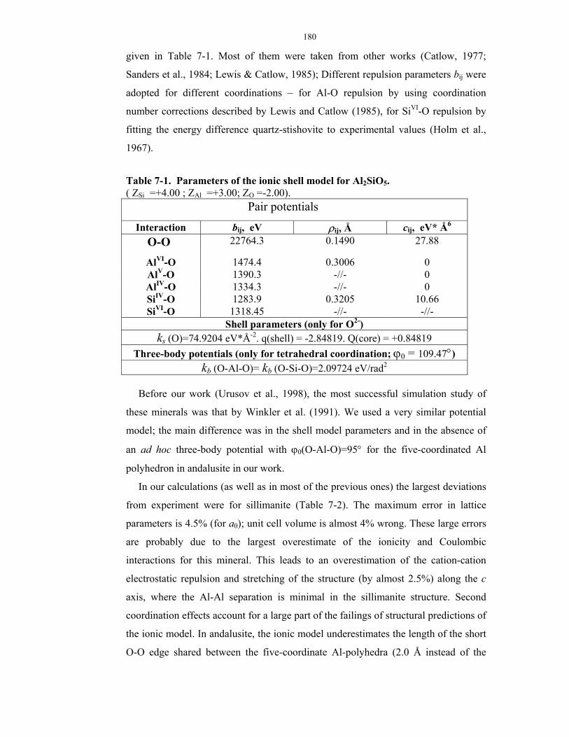
180
given in Table 7-1. Most of them were taken from other works (Catlow, 1977;
Sanders et al., 1984; Lewis & Catlow, 1985); Different repulsion parameters bij were
adopted for different coordinations – for Al-O repulsion by using coordination
number corrections described by Lewis and Catlow (1985), for SiVI-O repulsion by
fitting the energy difference quartz-stishovite to experimental values (Holm et al.,
1967).
Table 7-1. Parameters of the ionic shell model for Al2SiO5. ( ZSi =+4.00 ; ZAl =+3.00; ZO =-2.00). Pair potentials
Interaction bij, eV ρij, Å cij, eV* Å6 O-O 22764.3 0.1490 27.88
AlVI-O 1474.4 0.3006 0 AlV-O 1390.3 -//- 0 AlIV-O 1334.3 -//- 0 SiIV-O 1283.9 0.3205 10.66 SiVI-O 1318.45 -//- -//-
Shell parameters (only for O2-) ks (O)=74.9204 eV*Å-2. q(shell) = -2.84819. Q(core) = +0.84819
Three-body potentials (only for tetrahedral coordination; ϕ0 = 109.47°) kb (O-Al-O)= kb (O-Si-O)=2.09724 eV/rad2
Before our work (Urusov et al., 1998), the most successful simulation study of
these minerals was that by Winkler et al. (1991). We used a very similar potential
model; the main difference was in the shell model parameters and in the absence of
an ad hoc three-body potential with ϕ0(O-Al-O)=95° for the five-coordinated Al
polyhedron in andalusite in our work.
In our calculations (as well as in most of the previous ones) the largest deviations
from experiment were for sillimanite (Table 7-2). The maximum error in lattice
parameters is 4.5% (for a0); unit cell volume is almost 4% wrong. These large errors
are probably due to the largest overestimate of the ionicity and Coulombic
interactions for this mineral. This leads to an overestimation of the cation-cation
electrostatic repulsion and stretching of the structure (by almost 2.5%) along the c
axis, where the Al-Al separation is minimal in the sillimanite structure. Second
coordination effects account for a large part of the failings of structural predictions of
the ionic model. In andalusite, the ionic model underestimates the length of the short
O-O edge shared between the five-coordinate Al-polyhedra (2.0 Å instead of the
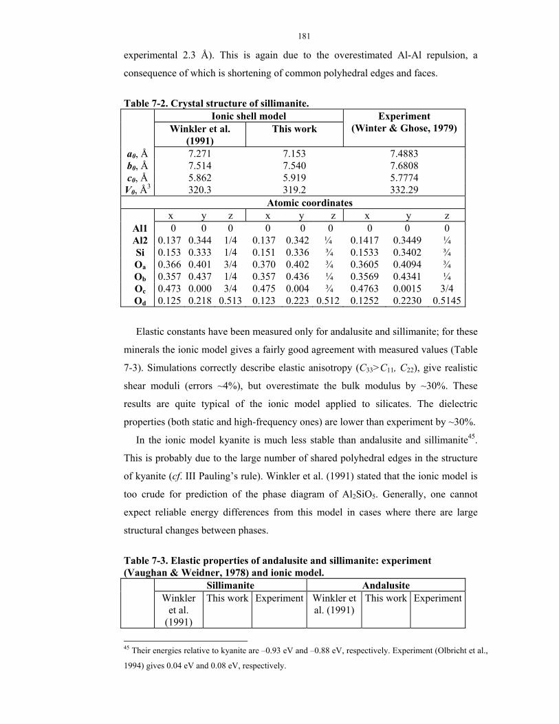
181
experimental 2.3 Å). This is again due to the overestimated Al-Al repulsion, a
consequence of which is shortening of common polyhedral edges and faces.
Table 7-2. Crystal structure of sillimanite.
Ionic shell model Winkler et al.
(1991) This work
Experiment (Winter & Ghose, 1979)
a0, Å 7.271 7.153 7.4883 b0, Å 7.514 7.540 7.6808 c0, Å 5.862 5.919 5.7774
V0, Å3 320.3 319.2 332.29 Atomic coordinates
x y z x y z x y z Al1 0 0 0 0 0 0 0 0 0 Al2 0.137 0.344 1/4 0.137 0.342 ¼ 0.1417 0.3449 ¼ Si 0.153 0.333 1/4 0.151 0.336 ¾ 0.1533 0.3402 ¾ Oa 0.366 0.401 3/4 0.370 0.402 ¾ 0.3605 0.4094 ¾ Ob 0.357 0.437 1/4 0.357 0.436 ¼ 0.3569 0.4341 ¼ Oc 0.473 0.000 3/4 0.475 0.004 ¾ 0.4763 0.0015 3/4 Od 0.125 0.218 0.513 0.123 0.223 0.512 0.1252 0.2230 0.5145
Elastic constants have been measured only for andalusite and sillimanite; for these
minerals the ionic model gives a fairly good agreement with measured values (Table
7-3). Simulations correctly describe elastic anisotropy (C33>C11, C22), give realistic
shear moduli (errors ~4%), but overestimate the bulk modulus by ~30%. These
results are quite typical of the ionic model applied to silicates. The dielectric
properties (both static and high-frequency ones) are lower than experiment by ~30%.
In the ionic model kyanite is much less stable than andalusite and sillimanite45.
This is probably due to the large number of shared polyhedral edges in the structure
of kyanite (cf. III Pauling’s rule). Winkler et al. (1991) stated that the ionic model is
too crude for prediction of the phase diagram of Al2SiO5. Generally, one cannot
expect reliable energy differences from this model in cases where there are large
structural changes between phases.
Table 7-3. Elastic properties of andalusite and sillimanite: experiment (Vaughan & Weidner, 1978) and ionic model.
Sillimanite Andalusite Winkler
et al. (1991)
This work Experiment Winkler et al. (1991)
This work Experiment
45 Their energies relative to kyanite are –0.93 eV and –0.88 eV, respectively. Experiment (Olbricht et al.,
1994) gives 0.04 eV and 0.08 eV, respectively.

182
Elastic constants (in GPa) C11 285 208 287.3 264 261 233.4 C22 277 278 231.9 254 361 289.0 C33 539 569 388.4 438 429 380.1 C44 130 135 122.4 85 83 99.5 C55 89 97 80.7 81 93 87.8 C66 85 57 89.3 120 107 112.3 C12 - 138 94.7 - 128 81.4 C13 - 138 83.4 - 171 116.2 C23 - 179 158.6 - 155 97.7
Voigt bulk and shear moduli (in GPa) KV - 218 175.1 - 217 165.9 GV - 98 95.1 - 97 100.4
Table 7-4 shows the results for the hypothetical phases. Both of them are much
less compressible than the real phases and higher in energy. The pseudobrookite
phase is unlikely to be stable at high pressures, because it is less dense than kyanite.
The V3O5–like phase spontaneously distorts in the ionic model and transforms into
another structure type. The resulting crystal structure has very high static dielectric
constants. These distortions are an artifact of the ionic model; partly covalent models
(Oganov, 1997; Oganov et al., 1997) and ab initio simulations (Oganov & Brodholt,
2000) do not find them.
A general conclusion is that the ionic shell model is in many cases semi-
quantitatively correct in predicting structures, elastic, and dielectric properties of
silicate minerals. It can also be useful in simulating lattice dynamics and defects. It is
generally not reliable in predictions of the energy differences between structurally
very different phases. Caution must be always paid, because structural predictions
can sometimes be qualitatively wrong. In ‘good’ cases the model leads to results
semiquantitatively similar to those of high-quality ab initio simulations (see Oganov
et al., 2001d and Chapter 9).
In the next chapter the performance of ab initio GGA simulations will be
analysed. These highly accurate simulations have helped us to resolve the long-
standing problem of high-pressure stability of the Al2SiO5 polymorphs.
Table 7-4. Ionic model predictions for the hypothetical high-pressure phases of Al2SiO5.
“V3O5-like” phase Pseudobrookite-like phase Lattice parameters
a0, Å 9.764 3.419 b0, Å 4.508 9.390
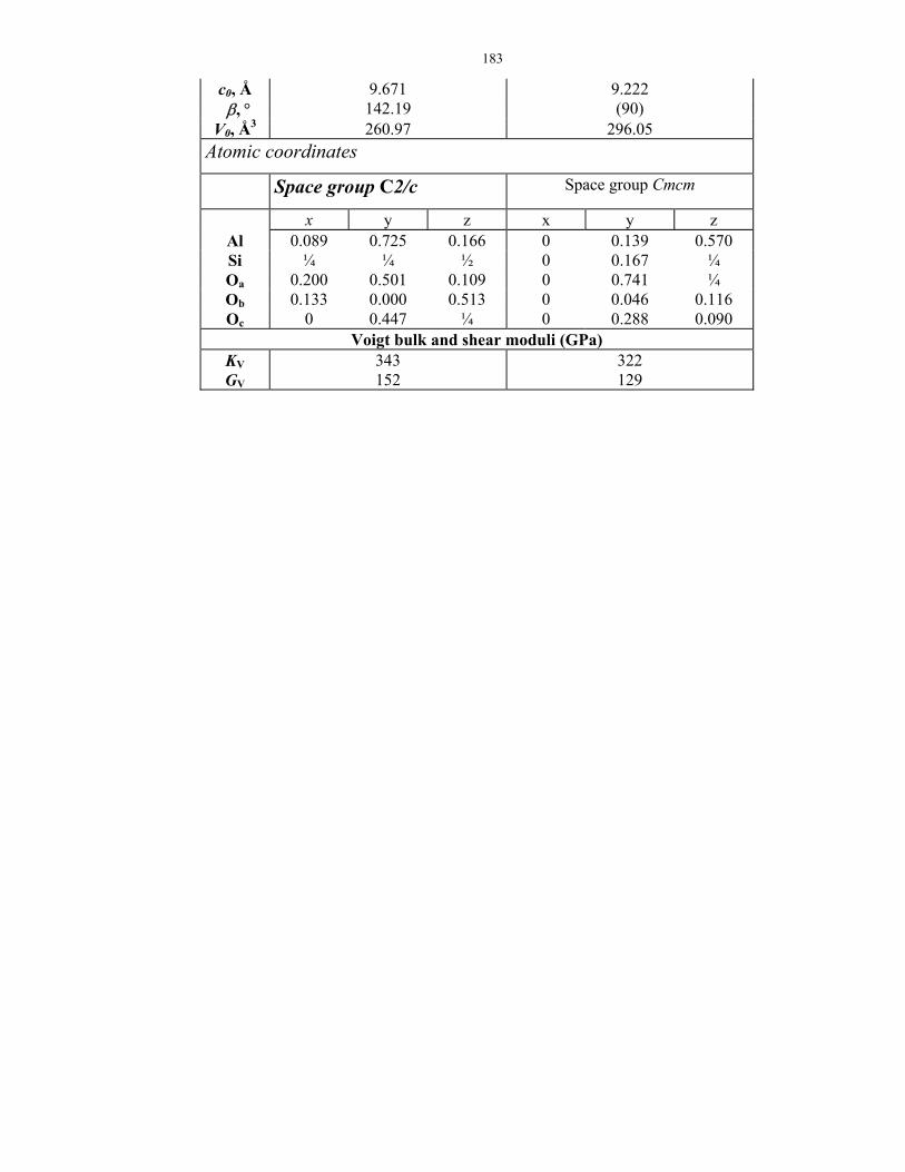
183
c0, Å 9.671 9.222 β, ° 142.19 (90)
V0, Å3 260.97 296.05 Atomic coordinates
Space group C2/c Space group Cmcm
x y z x y z Al 0.089 0.725 0.166 0 0.139 0.570 Si ¼ ¼ ½ 0 0.167 ¼ Oa 0.200 0.501 0.109 0 0.741 ¼ Ob 0.133 0.000 0.513 0 0.046 0.116 Oc 0 0.447 ¼ 0 0.288 0.090
Voigt bulk and shear moduli (GPa) KV 343 322 GV 152 129
184
Chapter 8. High-pressure stability of
Al2SiO5 and mineralogy of aluminium
in the Earth's lower mantle: ab initio
calculations.
As shown in the previous chapter, the ionic model is not accurate enough to be
used for calculating phase diagrams. Modern DFT can be used for such calculations.
In this chapter I show how DFT simulations have resolved the long-standing problem
of the high-pressure stability of the Al2SiO5 polymorphs discussed in the previous
chapter. The results presented here are from the paper by Oganov and Brodholt
(2000).
Ab initio GGA-DFT calculations have been performed using plane wave
pseudopotential method. Polymorphs of Al2SiO5 (kyanite, andalusite, sillimanite, and
hypothetical V3O5-like and pseudobrookite-like phases – see Fig. 8-1), SiO2
(stishovite, quartz) and Al2O3 (corundum) have been considered. Good agreement of
crystal structures, bulk moduli, atomisation energies and the phase diagram of
Al2SiO5 with experimental data was found. Strong disagreement between the
calculated lattice parameters and density of V3O5-like phase of Al2SiO5 and the
experimental values (Ahmed-Zaid & Madon, 1991) suggests that the phase studied in
the latter work is not a V3O5-structured phase of Al2SiO5. In addition, we found that
Al2SiO5 breaks down into the mixture of oxides at 11 GPa (at T=O K), in excellent
agreement with experimental estimates (9.5-15 GPa). The instability of Al2SiO5
phases with octahedrally coordinated Si to decomposition was explained on the basis
of Pauling’s second rule.
8.1. Computational methodology.
The calculations were performed with the VASP code (Kresse & Furthmuller,
1996a,b) and were based on DFT within the generalised gradient approximation
(PW91-GGA functional: Wang & Perdew (1991)). Valence electron wavefunctions
were expanded in plane-wave basis set and all core electrons replaced by effective
core pseudopotentials. All adopted pseudopotentials are non-local: norm-conserving

185
pseudopotentials (Rappe et al., 1990) with partial core corrections (Louie et al.,
1982) for Al and Si; non-normconserving (ultrasoft) pseudopotentials (Vanderbilt,
1990) for O. Core region cutoffs are 0.96 Å for Al (valence configuration 3s23p13d0),
0.95 Å for Si (valence configuration 3s23p23d0), and 0.82 Å for O (valence
configuration 2s22p43d0). All these pseudopotentials are supplied with the VASP
package.
a b
Fig. 8-1. Theoretically calculated crystal structures of the hypothetical high-
pressure phases of Al2SiO5. Si-polyhedra are grey, Al-polyhedra are light grey.
(a) V3O5-like structure. This structure is based on the hexagonal close packing of oxygen atoms.
Remarkable pairs of face-sharing octahedra tend to be occupied by Al rather than Si in order to reduce
the cation-cation electrostatic repulsion (3rd and 4th Pauling’s rules); this leads to the cation ordering
shown here and space group C2/c.
(b) Pseudobrookite-like structure. This structure is not close packed, but contains only fragments
(“islands”) of close packing. Therefore, its density cannot be very high: it should be close to the
density of the high-pressure Al2SiO5-melt. Interestingly, due to its topology, this structure in principle
cannot be built from ideal Al-octahedra.
The Al2SiO5-polymorphs are known to have very small energy differences (~0.04 eV
per formula unit at ambient conditions); the resulting kinetic problems precluded
precise experimental determination of the phase diagram of Al2SiO5 for a long time
(Zen, 1969; Kerrick, 1990). Therefore, care must be taken in order to reproduce these
small effects correctly and reliably.
A plane-wave cut-off energy of 800 eV proved to be very reliable (convergence to
within 6*10-4 eV/atom) and computationally acceptable; this was used throughout all
calculations. For Brillouin-zone sampling I used Monkhorst-Pack (1976) meshes:
4*4*4 for corundum (10 symmetrically unique points) and stishovite (6 unique
points), 3*3*3 for quartz (7 unique points), and 2*2*2 for all the Al2SiO5 phases (4
unique points for kyanite, 3 for V3O5-like phase, 2 for pseudobrookite-like phase,
and 1 unique point for andalusite and sillimanite). Increasing these numbers did not
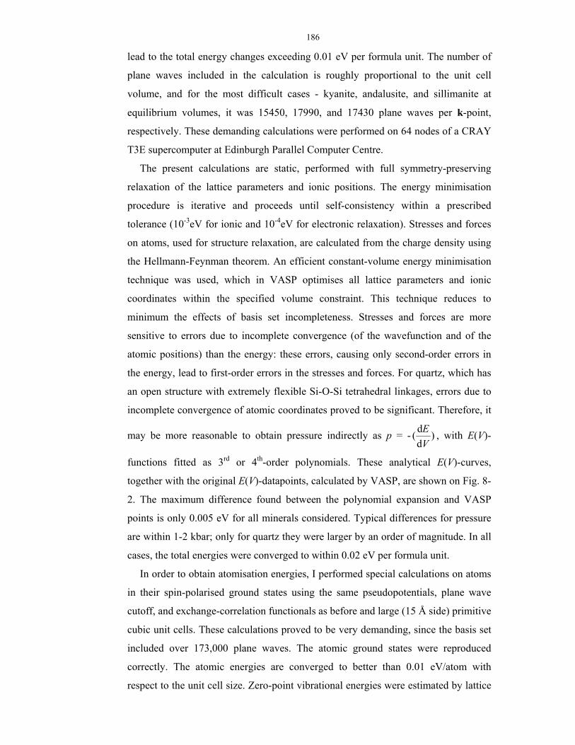
186
lead to the total energy changes exceeding 0.01 eV per formula unit. The number of
plane waves included in the calculation is roughly proportional to the unit cell
volume, and for the most difficult cases - kyanite, andalusite, and sillimanite at
equilibrium volumes, it was 15450, 17990, and 17430 plane waves per k-point,
respectively. These demanding calculations were performed on 64 nodes of a CRAY
T3E supercomputer at Edinburgh Parallel Computer Centre.
The present calculations are static, performed with full symmetry-preserving
relaxation of the lattice parameters and ionic positions. The energy minimisation
procedure is iterative and proceeds until self-consistency within a prescribed
tolerance (10-3eV for ionic and 10-4eV for electronic relaxation). Stresses and forces
on atoms, used for structure relaxation, are calculated from the charge density using
the Hellmann-Feynman theorem. An efficient constant-volume energy minimisation
technique was used, which in VASP optimises all lattice parameters and ionic
coordinates within the specified volume constraint. This technique reduces to
minimum the effects of basis set incompleteness. Stresses and forces are more
sensitive to errors due to incomplete convergence (of the wavefunction and of the
atomic positions) than the energy: these errors, causing only second-order errors in
the energy, lead to first-order errors in the stresses and forces. For quartz, which has
an open structure with extremely flexible Si-O-Si tetrahedral linkages, errors due to
incomplete convergence of atomic coordinates proved to be significant. Therefore, it
may be more reasonable to obtain pressure indirectly as p = - )dd(VE , with E(V)-
functions fitted as 3rd or 4th-order polynomials. These analytical E(V)-curves,
together with the original E(V)-datapoints, calculated by VASP, are shown on Fig. 8-
2. The maximum difference found between the polynomial expansion and VASP
points is only 0.005 eV for all minerals considered. Typical differences for pressure
are within 1-2 kbar; only for quartz they were larger by an order of magnitude. In all
cases, the total energies were converged to within 0.02 eV per formula unit.
In order to obtain atomisation energies, I performed special calculations on atoms
in their spin-polarised ground states using the same pseudopotentials, plane wave
cutoff, and exchange-correlation functionals as before and large (15 Å side) primitive
cubic unit cells. These calculations proved to be very demanding, since the basis set
included over 173,000 plane waves. The atomic ground states were reproduced
correctly. The atomic energies are converged to better than 0.01 eV/atom with
respect to the unit cell size. Zero-point vibrational energies were estimated by lattice
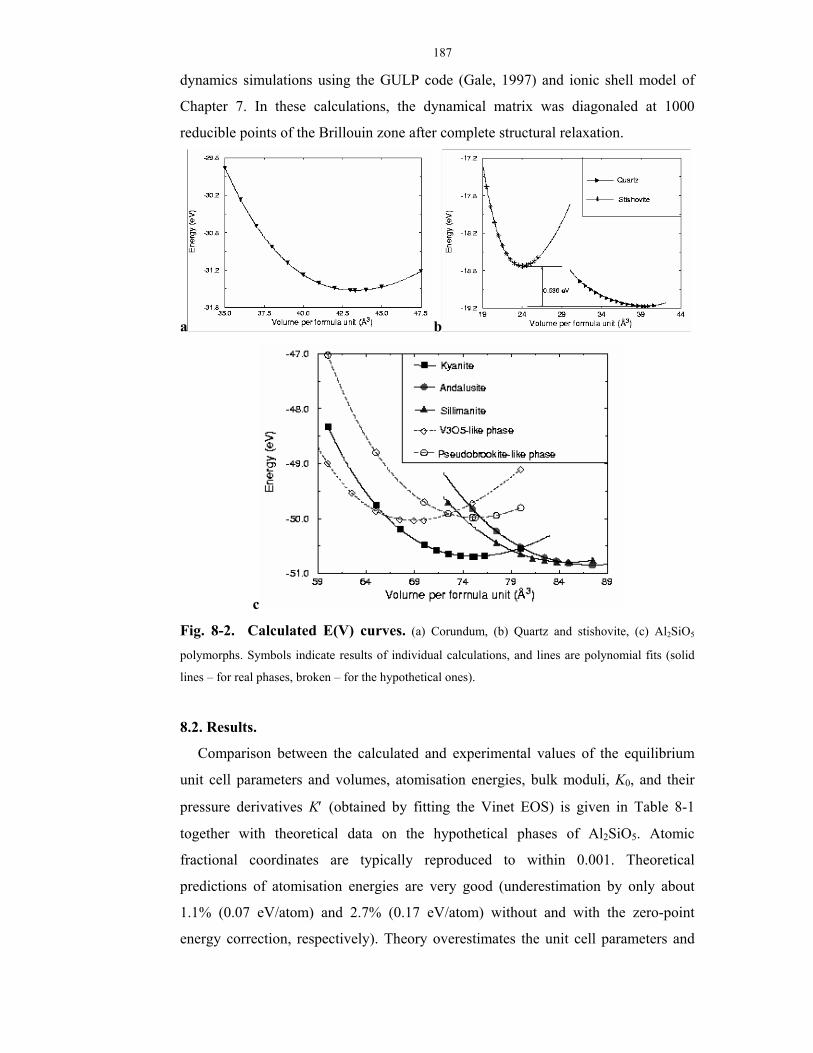
187
dynamics simulations using the GULP code (Gale, 1997) and ionic shell model of
Chapter 7. In these calculations, the dynamical matrix was diagonaled at 1000
reducible points of the Brillouin zone after complete structural relaxation.
a b
c
Fig. 8-2. Calculated E(V) curves. (a) Corundum, (b) Quartz and stishovite, (c) Al2SiO5
polymorphs. Symbols indicate results of individual calculations, and lines are polynomial fits (solid
lines – for real phases, broken – for the hypothetical ones).
8.2. Results.
Comparison between the calculated and experimental values of the equilibrium
unit cell parameters and volumes, atomisation energies, bulk moduli, K0, and their
pressure derivatives K′ (obtained by fitting the Vinet EOS) is given in Table 8-1
together with theoretical data on the hypothetical phases of Al2SiO5. Atomic
fractional coordinates are typically reproduced to within 0.001. Theoretical
predictions of atomisation energies are very good (underestimation by only about
1.1% (0.07 eV/atom) and 2.7% (0.17 eV/atom) without and with the zero-point
energy correction, respectively). Theory overestimates the unit cell parameters and
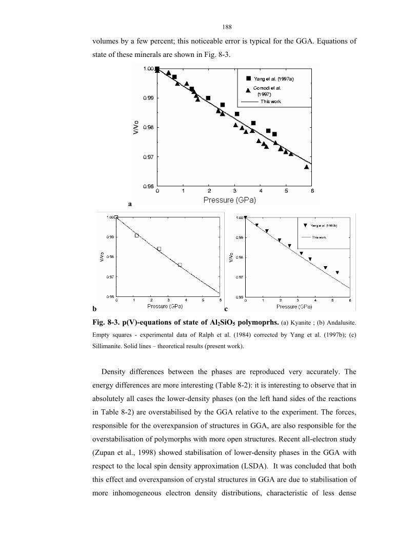
188
volumes by a few percent; this noticeable error is typical for the GGA. Equations of
state of these minerals are shown in Fig. 8-3.
a
b c
Fig. 8-3. p(V)-equations of state of Al2SiO5 polymoprhs. (a) Kyanite ; (b) Andalusite.
Empty squares - experimental data of Ralph et al. (1984) corrected by Yang et al. (1997b); (c)
Sillimanite. Solid lines – theoretical results (present work).
Density differences between the phases are reproduced very accurately. The
energy differences are more interesting (Table 8-2): it is interesting to observe that in
absolutely all cases the lower-density phases (on the left hand sides of the reactions
in Table 8-2) are overstabilised by the GGA relative to the experiment. The forces,
responsible for the overexpansion of structures in GGA, are also responsible for the
overstabilisation of polymorphs with more open structures. Recent all-electron study
(Zupan et al., 1998) showed stabilisation of lower-density phases in the GGA with
respect to the local spin density approximation (LSDA). It was concluded that both
this effect and overexpansion of crystal structures in GGA are due to stabilisation of
more inhomogeneous electron density distributions, characteristic of less dense
189
structures, by gradient corrections (see equation (5.3.4.11) and discussion there).
Results of all-electron calculations of Zupan et al. (1998) on quartz and stishovite
(structural parameters, K0 and K’) are in excellent agreement with our
pseudopotential study, highlighting very high quality of the pseudopotentials used in
our work.
As a consequence of the above discussed GGA error, in our calculations (as well
as in subsequent GGA calculations of Iglesias et al. (2001), but in contrast to
experiment) kyanite is not the thermodynamically stable phase at p=0 and T=0 K.
The application of pressure corrects this situation, increasing the relative stability of
the denser polymorphs. As a result, the phase diagram of Al2SiO5 (Fig. 8-4) is
reproduced very well, all the calculated transition pressures being only ~2 GPa
higher than the corresponding experimental values.
Figure 8-4. Phase diagram of Al2SiO5. Solid lines – experimental data, filled circles –
calculated transition pressures at T= 0 K, dashed lines were drawn through these points with
experimental p(T)-slopes of equilibria kyanite-(corundum+stishovite), kyanite-andalusite, and
kyanite-sillimanite. These data are suffiient to determine the p(T)-slope of andalusite-sillimanite
equilibrium.
Enthalpy vs pressure curves H(p) are represented in Fig. 8-5. From Fig. 8-2 and
Fig. 8-5 it is obvious that the pseudobrookite structure cannot be thermodynamically
stable for Al2SiO5 and becomes increasingly less stable at high pressures. It can also
be seen that kyanite, which in GGA simulations becomes the most stable phase at 1.9
GPa, transforms into the mixture of corundum and stishovite at 11 GPa (compare
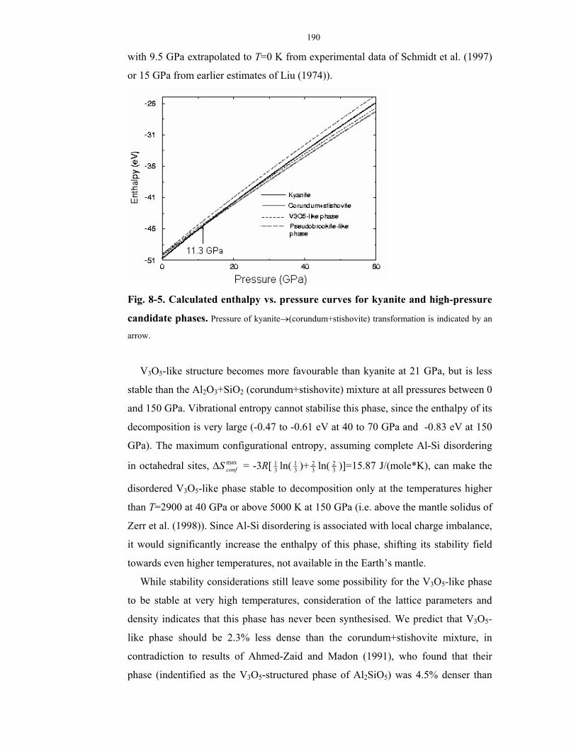
190
with 9.5 GPa extrapolated to T=0 K from experimental data of Schmidt et al. (1997)
or 15 GPa from earlier estimates of Liu (1974)).
Fig. 8-5. Calculated enthalpy vs. pressure curves for kyanite and high-pressure
candidate phases. Pressure of kyanite→(corundum+stishovite) transformation is indicated by an
arrow.
V3O5-like structure becomes more favourable than kyanite at 21 GPa, but is less
stable than the Al2O3+SiO2 (corundum+stishovite) mixture at all pressures between 0
and 150 GPa. Vibrational entropy cannot stabilise this phase, since the enthalpy of its
decomposition is very large (-0.47 to -0.61 eV at 40 to 70 GPa and -0.83 eV at 150
GPa). The maximum configurational entropy, assuming complete Al-Si disordering
in octahedral sites, ∆S maxconf
= -3R[ 31 ln( 3
1 )+ 32 ln( 3
2 )]=15.87 J/(mole*K), can make the
disordered V3O5-like phase stable to decomposition only at the temperatures higher
than T=2900 at 40 GPa or above 5000 K at 150 GPa (i.e. above the mantle solidus of
Zerr et al. (1998)). Since Al-Si disordering is associated with local charge imbalance,
it would significantly increase the enthalpy of this phase, shifting its stability field
towards even higher temperatures, not available in the Earth’s mantle.
While stability considerations still leave some possibility for the V3O5-like phase
to be stable at very high temperatures, consideration of the lattice parameters and
density indicates that this phase has never been synthesised. We predict that V3O5-
like phase should be 2.3% less dense than the corundum+stishovite mixture, in
contradiction to results of Ahmed-Zaid and Madon (1991), who found that their
phase (indentified as the V3O5-structured phase of Al2SiO5) was 4.5% denser than
191
the oxide mixture. The difference in the unit cell volume of the V3O5-like phase
between our calculations and results of Ahmed-Zaid and Madon (1991) is 11%,
which is well beyond the errors of the calculation. Lattice parameters, obtained in the
latter experiment, differ strikingly from ours (Table 8-1); however, care must be
taken since for monoclinic crystals (e.g., V3O5) three alternative settings of the
coordinate system - “cell choices” (International Tables for Crystallography, 1994))
- are possible. Simple matrix transformations allow one to change the cell choice. All
these cell choices are listed in Table 8-1. Cell choice 2 resembles results of Ahmed-
Zaid and Madon (1991) (a0 = 8.478 Å, b0 = 4.471 Å, c0 = 6.782 Å, β = 104.25°; V0 =
249.08 Å3) more than the others, however, the differences, especially in the a0-
parameter, are irreconciliable. Therefore, the phase synthesised by Ahmed-Zaid and
Madon (1991) is unlikely to be a V3O5-like polymorph of Al2SiO5.
I have also studied a variant of the V3O5-like structure with the space group P2/c,
differing in the distribution of Al and Si in octahedral sites. This structure, due to the
lower symmetry, has four (rather than two) non-equivalent cationic positions. This
variant can be produced from the C2/c–variant by exchanging positions of Si and one
half of Al atoms. This structure is much higher in energy than the C2/c-variant
(∆E=0.23 eV per formula unit) and somewhat less dense (∆V=0.30 cm3/mole).
Therefore, it should not be expected as a candidate high-pressure phase. Its
equilibrium lattice parameters are in a similarly striking disagreement with data of
Ahmed-Zaid and Madon (1991). The large value of ∆E=0.23 eV shows that the
energy cost of Al-Si disordering in this structure is high.
Based on the data from the paper by Ahmed-Zaid and Madon (1991) and on the
present results, we doubt that the Ahmed-Zaid and Madon’s phase is at all a
polymorph of Al2SiO5. A possibility, more consistent with the experimental unit cell
volume, is Al8Si3O8 (isochemical mixture of corundum and stishovite at ambient
pressure would have the molecular volume of 239.6 Å3). It should be possible to
determine, which structure and composition match the experimental lattice
parameters, using the newly developed genetic algorithms technique (Bush et al.,
1995).
8.3. Discussion.
Using ab initio calculations, we have demonstrated that kyanite, V3O5–like and
pseudobrookite-like phases of Al2SiO5 are unstable with respect to decomposition
192
into simple oxides, corundum (Al2O3) and stishovite (SiO2). It was recently
discovered that both corundum and stishovite are not the most stable phases of the
corresponding oxides at high pressures and should undergo phase transitions.
Corundum transforms into a phase with the Rh2O3(II)-type structure at 80-100 GPa
(experiment: Funamori & Jeanloz, 1997; theory: Marton & Cohen, 1994; Duan et al.,
1998), and stishovite transforms into a phase with the CaCl2-type structure at ca 50
GPa (experiment: Kingma et al., 1995; theory: Karki et al., 1997); there are also
theoretical predictions of further phase transitions for both minerals at higher
pressures. All these phase transitions occur at much higher pressures than the
decomposition of kyanite into corundum and stishovite (11 GPa) and, therefore, do
not change the calculated phase diagram, but only enhance our conclusion at very
high pressures, where even more stable oxide phases appear.
The results, concerning the hypothetical phases, can be rationalised in terms of
classical crystal chemistry. It turns out that the V3O5–like phase does not satisfy
Pauling’s second rule (sum of the electrostatic bond valences on the anion should be
equal to the anion’s valence). It is easy to check that this rule cannot be satisfied by
any composite phase in the Al2O3-SiO2 system with octahedrally coordinated Al and
Si. As has been shown by Brown (1992), structures that do not satisfy the second
Pauling’s rule must undergo distortions, quantified by the modified Pauling’s rule,
proposed by Brown (1992). Apart from such electronic effects as Jahn-Teller effect,
these distortions are usually destabilising. The distortion also results in an increase of
the average bond lengths (the “distortion theorem” (Brown, 1992) implied by
Brown’s rule), which may decrease the density of the structure. In contrast to V3O5–
like and pseudobrookite-like phases, corundum and stishovite satisfy Pauling’s rule
exactly. This partly explains the higher energy and lower density of the hypothetical
Al2SiO5-phases with respect to the mixture of corundum and stishovite.
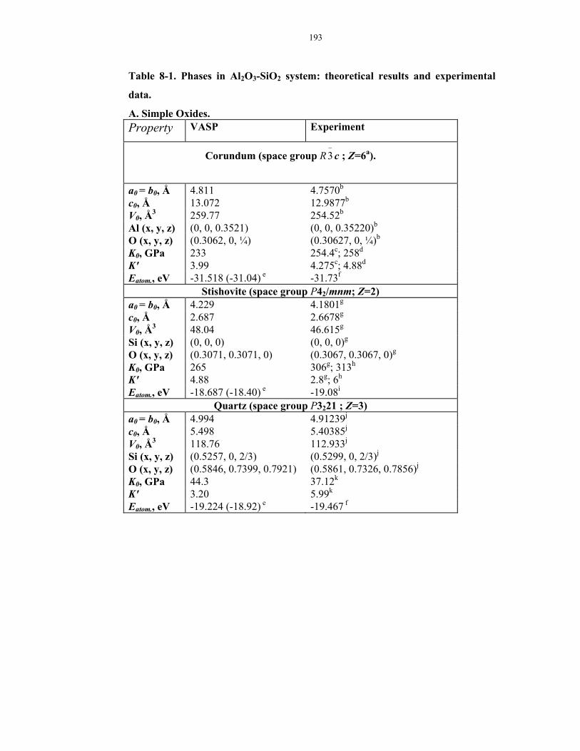
193
Table 8-1. Phases in Al2O3-SiO2 system: theoretical results and experimental
data.
A. Simple Oxides. Property VASP Experiment
Corundum (space group R−
3 c ; Z=6a).
a0 = b0, Å 4.811 4.7570b
c0, Å 13.072 12.9877b V0, Å3 259.77 254.52b Al (x, y, z) (0, 0, 0.3521) (0, 0, 0.35220)b O (x, y, z) (0.3062, 0, ¼) (0.30627, 0, ¼)b K0, GPa 233 254.4c; 258d K' 3.99 4.275c; 4.88d Eatom., eV -31.518 (-31.04) e -31.73f
Stishovite (space group P42/mnm; Z=2) a0 = b0, Å 4.229 4.1801g c0, Å 2.687 2.6678g V0, Å3 48.04 46.615g Si (x, y, z) (0, 0, 0) (0, 0, 0)g O (x, y, z) (0.3071, 0.3071, 0) (0.3067, 0.3067, 0)g K0, GPa 265 306g; 313h K' 4.88 2.8g; 6h Eatom., eV -18.687 (-18.40) e -19.08i
Quartz (space group P3221 ; Z=3) a0 = b0, Å 4.994 4.91239j c0, Å 5.498 5.40385j V0, Å3 118.76 112.933j Si (x, y, z) (0.5257, 0, 2/3) (0.5299, 0, 2/3)j O (x, y, z) (0.5846, 0.7399, 0.7921) (0.5861, 0.7326, 0.7856)j K0, GPa 44.3 37.12k K' 3.20 5.99k Eatom., eV -19.224 (-18.92) e -19.467 f

194
B. Known Al2SiO5 polymorphs. Property VASP Experiment
Kyanite (space group P1 ; Z=4).
a0 , Å 7.185 7.1262l b0, Å 7.916 7.8520l c0, Å 5.613 5.5724l α , ° 89.9 89.99l β , ° 101.1 101.11l γ , ° 106.0 106.03l V0, Å3 300.64 293.60l Al1 (x, y, z) (0.3247, 0.7039, 0.4581) (0.3254, 0.7040, 0.4582)l Al2 (x, y, z) (0.2966, 0.6986, 0.9502) (0.2974, 0.6989, 0.9505)l Al3 (x, y, z) (0.0994, 0.3864, 0.6407) (0.0998, 0.3862, 0.6403)l Al4 (x, y, z) (0.1116, 0.9170, 0.1645) (0.1120, 0.9175, 0.1649)l Si1 (x, y, z) (0.2961, 0.0650, 0.7066) (0.2962, 0.0649, 0.7066)l Si2 (x, y, z) (0.2909, 0.3315, 0.1896) (0.2910, 0.3317, 0.1892)l Oa (x, y, z) (0.1105, 0.1461, 0.1284) (0.1095, 0.1468, 0.1288)l Ob (x, y, z) (0.1230, 0.6858, 0.1816) (0.1230, 0.6856, 0.1812)l Oc (x, y, z) (0.2735, 0.4550, 0.9556) (0.2747, 0.4545, 0.9547)l Od (x, y, z) (0.2816, 0.9341, 0.9338) (0.2831, 0.9354, 0.9353)l Oe (x, y, z) (0.1218, 0.6300, 0.6389) (0.1219, 0.6307, 0.6389)l Of (x, y, z) (0.2810, 0.4447, 0.4289) (0.2822, 0.4453, 0.4288)l Og (x, y, z) (0.2901, 0.9465, 0.4658) (0.2915, 0.9467, 0.4659)l Oh (x, y, z) (0.5018, 0.2770, 0.2449) (0.5008, 0.2749, 0.2440)l Ok (x, y, z) (0.1091, 0.1532, 0.6682) (0.1084, 0.1520, 0.6669)l Om (x, y, z) (0.5024, 0.2298, 0.7560) (0.5015, 0.2312, 0.7553)l K0, GPa 172 156m ; 193n K' 4.01 5.6m ; [4]n Eatom., eV -50.692 (-49.91) e -51.27 f
Andalusite (space group Pnnm ; Z=4) a0 , Å 7.860 7.7980l b0, Å 7.956 7.9031l c0, Å 5.592 5.5566l V0, Å3 349.68 342.45l Al1 (x, y, z) (0, 0, 0.2419) (0, 0, 0.2419)l Al2 (x, y, z) (0.3709, 0.1389, ½) (0.3705, 0.1391, ½)l Si (x, y, z) (0.2458, 0.2522, 0) (0.2460, 0.2520, 0)l Oa (x, y, z) (0.4243, 0.3627, ½) (0.4233, 0.3629, ½)l Ob (x, y, z) (0.4238, 0.3640, 0) (0.4246, 0.3629, 0)l Oc (x, y, z) (0.1025, 0.4006, 0) (0.1030, 0.4003, 0)l Od (x, y, z) (0.2311, 0.1341, 0.2401) (0.2305, 0.1339, 0.2394)l K0, GPa 142 135o ; 151p K' 4.18 [4] o ; [4] p Eatom., eV -50.844 (-50.07) e -51.23 f
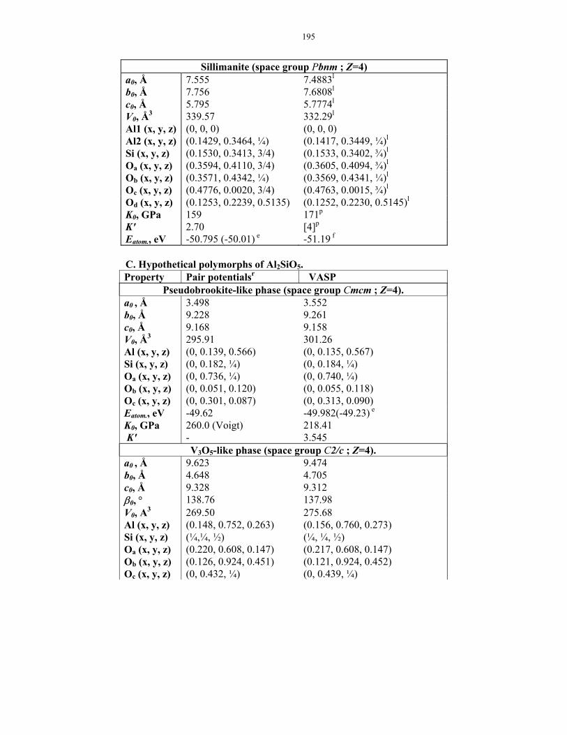
195
Sillimanite (space group Pbnm ; Z=4)
a0, Å 7.555 7.4883l b0, Å 7.756 7.6808l c0, Å 5.795 5.7774l V0, Å3 339.57 332.29l Al1 (x, y, z) (0, 0, 0) (0, 0, 0) Al2 (x, y, z) (0.1429, 0.3464, ¼) (0.1417, 0.3449, ¼)l Si (x, y, z) (0.1530, 0.3413, 3/4) (0.1533, 0.3402, ¾)l Oa (x, y, z) (0.3594, 0.4110, 3/4) (0.3605, 0.4094, ¾)l Ob (x, y, z) (0.3571, 0.4342, ¼) (0.3569, 0.4341, ¼)l Oc (x, y, z) (0.4776, 0.0020, 3/4) (0.4763, 0.0015, ¾)l Od (x, y, z) (0.1253, 0.2239, 0.5135) (0.1252, 0.2230, 0.5145)l K0, GPa 159 171p K' 2.70 [4]p Eatom., eV -50.795 (-50.01) e -51.19 f C. Hypothetical polymorphs of Al2SiO5. Property Pair potentialsr VASP
Pseudobrookite-like phase (space group Cmcm ; Z=4). a0 , Å 3.498 3.552 b0, Å 9.228 9.261 c0, Å 9.168 9.158 V0, Å3 295.91 301.26 Al (x, y, z) (0, 0.139, 0.566) (0, 0.135, 0.567) Si (x, y, z) (0, 0.182, ¼) (0, 0.184, ¼) Oa (x, y, z) (0, 0.736, ¼) (0, 0.740, ¼) Ob (x, y, z) (0, 0.051, 0.120) (0, 0.055, 0.118) Oc (x, y, z) (0, 0.301, 0.087) (0, 0.313, 0.090) Eatom., eV -49.62 -49.982(-49.23) e K0, GPa 260.0 (Voigt) 218.41 K' - 3.545
V3O5-like phase (space group C2/c ; Z=4). a0 , Å 9.623 9.474 b0, Å 4.648 4.705 c0, Å 9.328 9.312 β0, ° 138.76 137.98 V0, A3 269.50 275.68 Al (x, y, z) (0.148, 0.752, 0.263) (0.156, 0.760, 0.273) Si (x, y, z) (¼,¼, ½) (¼, ¼, ½) Oa (x, y, z) (0.220, 0.608, 0.147) (0.217, 0.608, 0.147) Ob (x, y, z) (0.126, 0.924, 0.451) (0.121, 0.924, 0.452) Oc (x, y, z) (0, 0.432, ¼) (0, 0.439, ¼)
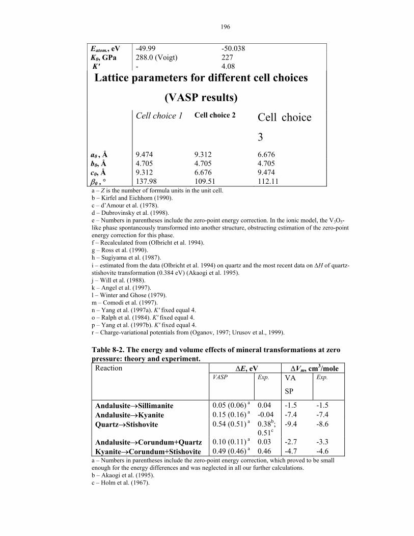
196
Eatom., eV -49.99 -50.038 K0, GPa 288.0 (Voigt) 227 K' - 4.08 Lattice parameters for different cell choices
(VASP results) Cell choice 1 Cell choice 2 Cell choice
3 a0 , Å 9.474 9.312 6.676 b0, Å 4.705 4.705 4.705 c0, Å 9.312 6.676 9.474 β0 , ° 137.98 109.51 112.11 a – Z is the number of formula units in the unit cell. b – Kirfel and Eichhorn (1990). c – d’Amour et al. (1978). d – Dubrovinsky et al. (1998). e – Numbers in parentheses include the zero-point energy correction. In the ionic model, the V3O5-like phase spontaneously transformed into another structure, obstructing estimation of the zero-point energy correction for this phase. f – Recalculated from (Olbricht et al. 1994). g – Ross et al. (1990). h – Sugiyama et al. (1987). i – estimated from the data (Olbricht et al. 1994) on quartz and the most recent data on ∆H of quartz-stishovite transformation (0.384 eV) (Akaogi et al. 1995). j – Will et al. (1988). k – Angel et al. (1997). l – Winter and Ghose (1979). m – Comodi et al. (1997). n – Yang et al. (1997a). K' fixed equal 4. o – Ralph et al. (1984). K' fixed equal 4. p – Yang et al. (1997b). K' fixed equal 4. r – Charge-variational potentials from (Oganov, 1997; Urusov et al., 1999). Table 8-2. The energy and volume effects of mineral transformations at zero pressure: theory and experiment.
∆E, eV ∆Vm, cm3/mole Reaction VASP Exp. VA
SP
Exp.
Andalusite→Sillimanite 0.05 (0.06) a 0.04 -1.5 -1.5 Andalusite→Kyanite 0.15 (0.16) a -0.04 -7.4 -7.4 Quartz→Stishovite 0.54 (0.51) a 0.38b;
0.51c -9.4 -8.6
Andalusite→Corundum+Quartz 0.10 (0.11) a 0.03 -2.7 -3.3 Kyanite→Corundum+Stishovite 0.49 (0.46) a 0.46 -4.7 -4.6
a – Numbers in parentheses include the zero-point energy correction, which proved to be small enough for the energy differences and was neglected in all our further calculations. b – Akaogi et al. (1995). c – Holm et al. (1967).
197
On the other hand, it is well known that the formation of complex oxides and
silicates from the constituent oxides is favoured when cations differ significantly in
the electronegativities (Urusov, 1993) and ionic radii (e.g., MgO+SiO2→ MgSiO3
due to significant differences in the electronegativities and ionic radii of Mg and Si).
In other terms, the formation of the complex compounds is strongly favoured if the
constituent components have different acid-base properties and can play different
crystal-chemical roles. At high pressures, both Si4+ and Al3+ adopt octahedral
coordination and cannot play significantly different structural roles anymore. As a
result, pure Al-silicates are likely to break down, as in the case considered here. In
contrast, aluminosilicates of large and electropositive cations (Ca, Mg, Na, K), e.g.
the hollandite-like phase of (Ca,Mg)Al2Si2O8, or the high-pressure modifications of
MgAl2O4, could be stable in the lower mantle and be major hosts of Al in the lower
mantle, unless Al prefers to form (Mg,Fe)(Si,Al)O3-perovskite solid solutions46.
In the next chapter I discuss the compression behaviour of the Al2SiO5
polymorphs simulated by ab initio and semiclassical methods. Their anomalous
behaviour at high pressures gives much insight into the nature of pressure-induced
phase transitions and metastability.
46 Note, however, that both arguments (Pauling’s second rule and acid-base properties of cations) are
purely energetical and do not apply to the entropy. Although the octahedral Al-silicates are
unfavoured energetically, they may be stabilised by the configurational entropy of Al-Si disorder at
high temperatures. In the particular case of the V3O5–like modification of Al2SiO5 we have shown
that the lower mantle temperatures are insufficient to stabilise it. One can expect that Al-Si
disordering in (Mg,Fe)(Si,Al)O3-perovskite, where Al is a minor element, would produce a greater net
entropical effect than in any phase with both Al and Si as major components.
198
Chapter 9. Metastable Al2SiO5
polymorphs.
The previous chapter demonstrated the high accuracy and reliability of DFT
simulations. These simulations showed that all Al2SiO5 polymorphs become
thermodynamically unstable with respect to decomposition into the mixture of
constituent oxides above 11 GPa. Here I investigate the compression behaviour of
the Al2SiO5 polymorphs in the pressure regime where they are metastable. Static
DFT simulations are used in parallel with lattice dynamics simulations based on the
ionic shell model. The results presented here are from the paper by Oganov et al.
(2001d).
I predict a series of metastable phase transitions occurring in low-pressure
Al2SiO5 polymorphs (andalusite and sillimanite); similar results were obtained using
DFT simulations and semiclassical calculations using the ionic shell model. Soft
lattice modes as well as related structural changes are analysed. For sillimanite, I
predict an isosymmetric phase transition at ca 35 GPa; an incommensurately
modulated form of sillimanite can also be obtained at low temperatures and high
pressures. The high-pressure isosymmetric phase contains five-coordinate Si and Al
atoms. The origin of this peculiar fivefold coordination is discussed in detail.
Andalusite was found to transform into an amorphous phase at ~50 GPa. This study
provides insight into the nature of metastable modifications of crystal structures and
the ways in which they are formed. Present results indicate the existence of a critical
bonding distance, above which interatomic contacts cannot be considered as bonds.
The critical distance for the Si-O bonds is 2.25 Å.
9.1. Introduction.
Metastability phenomena play an important role in many natural and
technological processes. Metastable phases are often obtained in synthesis and as
products of phase transformations. Recent discoveries, e.g. of pressure-induced
amorphisation by Mishima et al. (1984) and the memory glass effect by Kruger and
Jeanloz (1990), have boosted interest in metastability phenomena. It is possible, for
instance, that ice comets to a large extent are made of amorphous ice phases, formed
at high pressure and low temperatures. Another example is provided by isosymmetric
199
phase transitions, which can lead to both stable (e.g., KTiOPO4, see Alan & Nelmes,
1996) and metastable (e.g., SiO2, Badro et al., 1996) phases. This type of phase
transitions, until recently thought to be very unusual, is now being found in an
increasing number of systems.
Here I discuss state-of-the-art theoretical simulations of metastable phases in the
Al2SiO5 system. A variety of metastable phases predicted here make Al2SiO5 an
ideal subject for studies of metastable phenomena.
Both experiments (Schmidt et al., 1997) and theory (Oganov & Brodholt, 2000)
indicate that above ~10 GPa Al2SiO5 phases become thermodynamically unstable
and decompose into the mixture of oxides, Al2O3+SiO2. However, as metastable
phases they can exist up to much higher pressures. Kyanite, whose dense structure is
based upon cubic closest packing of oxygen atoms, can persist as a metastable phase
up to at least 80 GPa; the same is true for the hypothetical dense pseudobrookite-like
and V3O5-like phases of Al2SiO5 (Oganov & Brodholt, 2000). Using ab initio
simulations, I have found that the low-density phases, andalusite and sillimanite,
spontaneously undergo extremely interesting phase transitions in the region 35-55
GPa. These transitions will be considered below.
9.2. Computational methodology.
Two distinct computer simulation methods were employed: 1) first principles
pseudopotential calculations and 2) semiclassical calculations, based on empirically
derived interatomic potentials. Quantum-mechanical calculations are very accurate
and reliable, but computationally expensive. Their results comprise the main
quantitative basis for discussion of structural and thermodynamic aspects of the
phase transitions. More approximate semi-classical calculations, which are very
cheap in terms of CPU time (about 103 times faster than the first principles
calculations), can be used efficiently for dynamical as well as for static calculations.
This technique is employed here for studying dynamical properties at a qualitative
level.
Theoretically, a structure can be metastable at given conditions if there are no net
forces acting on atoms at rest, and there are no soft modes. As present calculations
show, andalusite and sillimanite can persist as metastable phases up to ~35-55 GPa;
at these pressures they cease to be in the local energy minima (soft modes appear),
and spontaneously transform into other metastable phases.

200
First-principles calculations were performed on the Cray T3E supercomputers at
Edinburgh Parallel Computer Centre and Manchester Computer Centre. The
computational method was described in Chapter 8. The main difference is that the
present calculations were performed using the constant-pressure enthalpy
minimisation algorithm. This was done iteratively until self-consistency to within 10-
3 eV for ionic and 10-4 eV for electronic relaxation was achieved.
Semiclassical calculations were performed with the GULP package. Lattice
dynamics is a key point in theory of phase transitions. Unfortunately, non-empirical
calculations are currently computationally too demanding to be routinely used for
lattice dynamics, especially in the case of low-symmetry ionic crystals with large
unit cells.
The performance of the ionic shell model was analysed in Chapter 7. This model
is known to have serious drawbacks, but at the same time in a large number of cases,
including the Al2SiO5 polymorphs (Winkler & Buehrer, 1990; Rao et al., 1999),
proved to be sufficiently good at describing lattice dynamics of silicate minerals
(Burnham, 1990). In my calculations the Buckingham potentials were summed over
all interatomic pairs with distances below 10 Å; three-body potentials were
calculated only between strong bonds (shorter than 1.8 Å for Si-O and 1.9 Å for Al-O
bonds). Three-body terms are important for tetrahedrally coordinated silicates. For
consistency I use the same ‘tetrahedral’ three-body terms even for non-tetrahedral
high-pressure structures, even though this can lead to some ambiguity.
9.3. Accuracy of simulations.
It is known that semiclassical calculations are unreliable in predicting phase
transformation enthalpies, when large structural changes are involved, e.g. for
transitions between kyantite, andalusite, and sillimanite (Winkler et al., 1991;
Urusov et al., 1998). Ab initio GGA calculations, on the other hand, successfully
reproduce the phase diagram (Fig. 8-4) of the Al2SiO5 system (Oganov & Brodholt,
2000). However, both methods give a very similar qualitative picture of the
metastable and largely structure-conserving pressure-induced phase transitions in
andalusite and sillimanite. Only the transition pressures predicted by semiclassical
calculations are ~2 times lower than the GGA values. Although the GGA usually
results in a shifted pressure scale (Oganov et al., 2001a) and often overestimates
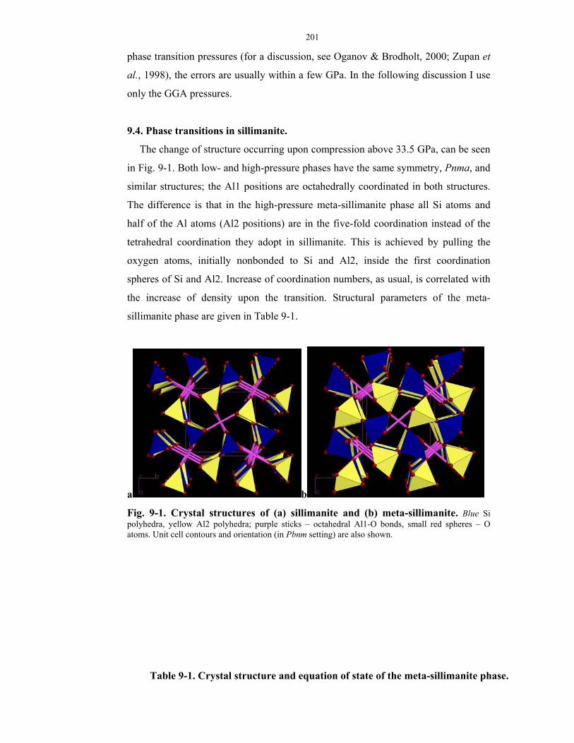
201
phase transition pressures (for a discussion, see Oganov & Brodholt, 2000; Zupan et
al., 1998), the errors are usually within a few GPa. In the following discussion I use
only the GGA pressures.
9.4. Phase transitions in sillimanite.
The change of structure occurring upon compression above 33.5 GPa, can be seen
in Fig. 9-1. Both low- and high-pressure phases have the same symmetry, Pnma, and
similar structures; the Al1 positions are octahedrally coordinated in both structures.
The difference is that in the high-pressure meta-sillimanite phase all Si atoms and
half of the Al atoms (Al2 positions) are in the five-fold coordination instead of the
tetrahedral coordination they adopt in sillimanite. This is achieved by pulling the
oxygen atoms, initially nonbonded to Si and Al2, inside the first coordination
spheres of Si and Al2. Increase of coordination numbers, as usual, is correlated with
the increase of density upon the transition. Structural parameters of the meta-
sillimanite phase are given in Table 9-1.
a b
Fig. 9-1. Crystal structures of (a) sillimanite and (b) meta-sillimanite. Blue Si polyhedra, yellow Al2 polyhedra; purple sticks – octahedral Al1-O bonds, small red spheres – O atoms. Unit cell contours and orientation (in Pbnm setting) are also shown.
Table 9-1. Crystal structure and equation of state of the meta-sillimanite phase.
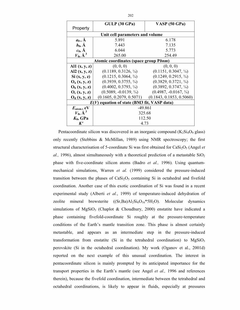
202
Pentacoordinate silicon was discovered in an inorganic compound (K2Si4O9 glass)
only recently (Stebbins & McMillan, 1989) using NMR spectroscopy; the first
structural characterisation of 5-coordinate Si was first obtained for CaSi2O5 (Angel et
al., 1996), almost simultaneously with a theoretical prediction of a metastable SiO2
phase with five-coordinate silicon atoms (Badro et al., 1996). Using quantum-
mechanical simulations, Warren et al. (1999) considered the pressure-induced
transition between the phases of CaSi2O5 containing Si in octahedral and fivefold
coordination. Another case of this exotic coordination of Si was found in a recent
experimental study (Alberti et al., 1999) of temperature-induced dehydration of
zeolite mineral brewsterite ((Sr,Ba)Al2Si6O16*5H2O). Molecular dynamics
simulations of MgSiO3 (Chaplot & Choudhury, 2000) enstatite have indicated a
phase containing fivefold-coordinate Si roughly at the pressure-temperature
conditions of the Earth’s mantle transition zone. This phase is almost certainly
metastable, and appears as an intermediate step in the pressure-induced
transformation from enstatite (Si in the tetrahedral coordination) to MgSiO3
perovskite (Si in the octahedral coordination). My work (Oganov et al., 2001d)
reported on the next example of this unusual coordination. The interest in
pentacoordinate silicon is mainly prompted by its anticipated importance for the
transport properties in the Earth’s mantle (see Angel et al., 1996 and references
therein), because the fivefold coordination, intermediate between the tetrahedral and
octahedral coordinations, is likely to appear in fluids, especially at pressures
Property GULP (30 GPa) VASP (50 GPa)
Unit cell parameters and volume a0 , Å 5.891 6.178 b0, Å 7.443 7.135 c0, Å 6.044 5.773
V0, Å 3 265.00 254.49 Atomic coordinates (space group Pbnm)
Al1 (x, y, z) (0, 0, 0) (0, 0, 0) Al2 (x, y, z) (0.1189, 0.3126, ¼) (0.1151, 0.3047, ¼) Si (x, y, z) (0.1215, 0.3064, ¾) (0.1249, 0.2915, ¾) Oa (x, y, z) (0.3939, 0.3755, ¾) (0.3829, 0.3721, ¾) Ob (x, y, z) (0.4002, 0.3793, ¼) (0.3892, 0.3747, ¼) Oc (x, y, z) (0.5089, -0.0139, ¾) (0.4987, -0.0167, ¾) Od (x, y, z) (0.1605, 0.2079, 0.5071) (0.1843, 0.1853, 0.5060)
E(V) equation of state (BM3 fit, VASP data) Eatom., eV -49.861
V0, Å 3 325.68 K0, GPa 112.50
K' 4.73
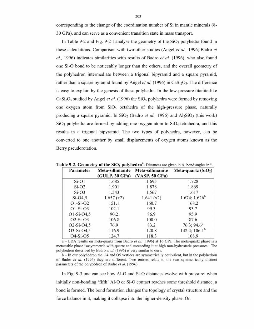
203
corresponding to the change of the coordination number of Si in mantle minerals (8-
30 GPa), and can serve as a convenient transition state in mass transport.
In Table 9-2 and Fig. 9-2 I analyse the geometry of the SiO5 polyhedra found in
these calculations. Comparison with two other studies (Angel et al., 1996; Badro et
al., 1996) indicates similarities with results of Badro et al. (1996), who also found
one Si-O bond to be noticeably longer than the others, and the overall geometry of
the polyhedron intermediate between a trigonal bipyramid and a square pyramid,
rather than a square pyramid found by Angel et al. (1996) in CaSi2O5. The difference
is easy to explain by the genesis of these polyhedra. In the low-pressure titanite-like
CaSi2O5 studied by Angel et al. (1996) the SiO5 polyhedra were formed by removing
one oxygen atom from SiO6 octahedra of the high-pressure phase, naturally
producing a square pyramid. In SiO2 (Badro et al., 1996) and Al2SiO5 (this work)
SiO5 polyhedra are formed by adding one oxygen atom to SiO4 tetrahedra, and this
results in a trigonal bipyramid. The two types of polyhedra, however, can be
converted to one another by small displacements of oxygen atoms known as the
Berry pseudorotation.
Table 9-2. Geometry of the SiO5 polyhedraa. Distances are given in Å, bond angles in °.
a – LDA results on meta-quartz from Badro et al. (1996) at 16 GPa. The meta-quartz phase is a metastable phase isosymmetric with quartz and succeeding it at high non-hydrostatic pressures. The polyhedron described by Badro et al. (1996) is very similar to ours.
b – In our polyhedron the O4 and O5 vertices are symmetrically equivalent, but in the polyhedron of Badro et al. (1996) they are different. Two entries relate to the two symmetrically distinct parameters of the polyhedron of Badro et al. (1996).
In Fig. 9-3 one can see how Al-O and Si-O distances evolve with pressure: when
initially non-bonding ‘fifth’ Al-O or Si-O contact reaches some threshold distance, a
bond is formed. The bond formation changes the topology of crystal structure and the
force balance in it, making it collapse into the higher-density phase. On
Parameter Meta-sillimanite(GULP, 30 GPa)
Meta-sillimanite (VASP, 50 GPa)
Meta-quartz (SiO2)
Si-O1 1.685 1.695 1.728 Si-O2 1.901 1.878 1.869 Si-O3 1.543 1.567 1.617
Si-O4,5 1.657 (x2) 1.641 (x2) 1.674; 1.626b O1-Si-O2 151.1 160.7 168.2 O1-Si-O3 102.1 99.3 93.7
O1-Si-O4,5 90.2 86.9 95.9 O2-Si-O3 106.8 100.0 87.6
O2-Si-O4,5 76.9 83.2 76.3; 94.6b O3-Si-O4,5 116.9 120.8 142.4; 106.1b O4-Si-O5 124.7 118.3 108.9
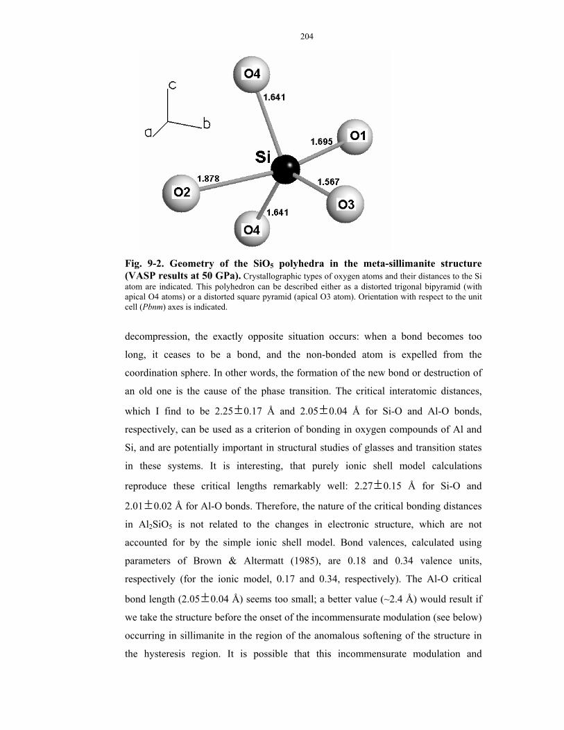
204
Fig. 9-2. Geometry of the SiO5 polyhedra in the meta-sillimanite structure (VASP results at 50 GPa). Crystallographic types of oxygen atoms and their distances to the Si atom are indicated. This polyhedron can be described either as a distorted trigonal bipyramid (with apical O4 atoms) or a distorted square pyramid (apical O3 atom). Orientation with respect to the unit cell (Pbnm) axes is indicated.
decompression, the exactly opposite situation occurs: when a bond becomes too
long, it ceases to be a bond, and the non-bonded atom is expelled from the
coordination sphere. In other words, the formation of the new bond or destruction of
an old one is the cause of the phase transition. The critical interatomic distances,
which I find to be 2.25 ±0.17 Å and 2.05 ±0.04 Å for Si-O and Al-O bonds,
respectively, can be used as a criterion of bonding in oxygen compounds of Al and
Si, and are potentially important in structural studies of glasses and transition states
in these systems. It is interesting, that purely ionic shell model calculations
reproduce these critical lengths remarkably well: 2.27±0.15 Å for Si-O and
2.01±0.02 Å for Al-O bonds. Therefore, the nature of the critical bonding distances
in Al2SiO5 is not related to the changes in electronic structure, which are not
accounted for by the simple ionic shell model. Bond valences, calculated using
parameters of Brown & Altermatt (1985), are 0.18 and 0.34 valence units,
respectively (for the ionic model, 0.17 and 0.34, respectively). The Al-O critical
bond length (2.05±0.04 Å) seems too small; a better value (~2.4 Å) would result if
we take the structure before the onset of the incommensurate modulation (see below)
occurring in sillimanite in the region of the anomalous softening of the structure in
the hysteresis region. It is possible that this incommensurate modulation and
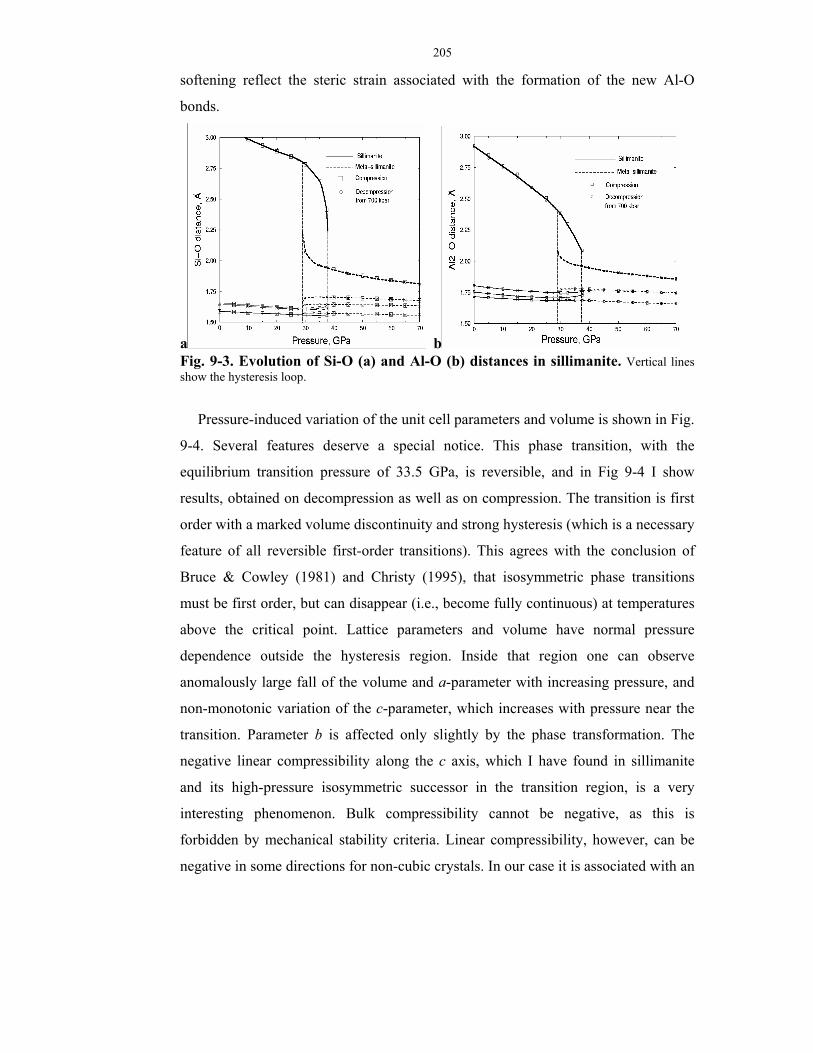
205
softening reflect the steric strain associated with the formation of the new Al-O
bonds.
a b Fig. 9-3. Evolution of Si-O (a) and Al-O (b) distances in sillimanite. Vertical lines show the hysteresis loop.
Pressure-induced variation of the unit cell parameters and volume is shown in Fig.
9-4. Several features deserve a special notice. This phase transition, with the
equilibrium transition pressure of 33.5 GPa, is reversible, and in Fig 9-4 I show
results, obtained on decompression as well as on compression. The transition is first
order with a marked volume discontinuity and strong hysteresis (which is a necessary
feature of all reversible first-order transitions). This agrees with the conclusion of
Bruce & Cowley (1981) and Christy (1995), that isosymmetric phase transitions
must be first order, but can disappear (i.e., become fully continuous) at temperatures
above the critical point. Lattice parameters and volume have normal pressure
dependence outside the hysteresis region. Inside that region one can observe
anomalously large fall of the volume and a-parameter with increasing pressure, and
non-monotonic variation of the c-parameter, which increases with pressure near the
transition. Parameter b is affected only slightly by the phase transformation. The
negative linear compressibility along the c axis, which I have found in sillimanite
and its high-pressure isosymmetric successor in the transition region, is a very
interesting phenomenon. Bulk compressibility cannot be negative, as this is
forbidden by mechanical stability criteria. Linear compressibility, however, can be
negative in some directions for non-cubic crystals. In our case it is associated with an

206
incipient phase transition and formation/breaking of new bonds in the structure47.
This isosymmetric transition is ferroelastic, because it is associated (as shown by
GULP calculations) with a complete softening of the C11 elastic constant. This
correlates with the collapse of the a axis, associated with the formation of new Si-O
and Al-O bonds directed largely along the a direction.
a b Fig. 9-4. Pressure evolution of (a) lattice parameters and (b) volume of sillimanite. Hysteresis loop is very pronounced.
Variation of the lattice parameters in the vicinity of the transition suggests that
structures of the both phases ‘prepare’ for the transition, i.e. their lattice parameters
tend to merge towards the transition. It is well known (Sirotin & Shaskolskaya, 1975)
that for structural transitions with symmetry breaking, structure of the low-symmetry
phase becomes increasingly more similar to the high-symmetry structure, whereas the
latter shows no indication of approaching the low-symmetry structure. As our example
suggests, in cases when symmetry of the phases is identical, both structures show a
tendency to approach each other in the vicinity of the transition.
Using semi-classical simulations, I considered dynamical stability criteria (Fig. 9-
5). At ambient pressure, sillimanite is dynamically stable, in agreement with
experiment. The high-pressure isosymmetric phase is also dynamically stable.
However, ca 1 GPa below the high-pressure transition sillimanite acquires a minor
47 In Pb3(PO4)2 negative linear compressibility was found along the c direction of the monoclinic cell
(Angel, 2000); it was tentatively ascribed to the stereochemical activity of lone electron pair of Pb2+
(R.J. Angel, private communication).

207
dynamical instability, which would lead to an incommensurate modulation with
k≈(0.47,0,0) (Fig. 9-5b). The imaginary frequencies are very small, suggesting that
the modulation may be anharmonically suppressed even at not very high
temperatures, and the isosymmetric phase transition would occur bypassing the
incommensurate phase.
a b
c Fig. 9-5. Phonon dispersion curves of sillimanite under pressure. (a) Sillimanite at room pressure, (b) sillimanite near the transition to the isosymmetric phase, (b)isosymmetric phase. Only several lowest-frequency phonon branches are shown. Pbnm setting is used in the notation of reciprocal space points.
Several spot-checks were performed using both VASP and GULP, in order to
make sure that the input structure did not bias the results. These spot-checks started
with a slightly deformed (by 0.01-0.02 Å and 1-2º) unit cell and displaced atoms (by
0.01-0.02 Å) picked at random, followed by static constant-pressure relaxation of the
structure. For the high-pressure meta-sillimanite modification the original structure

208
was always recovered in VASP calculations even at pressures as high as 70 GPa. At
the same time, ~10 GPa after the formation of the isosymmetric phase, GULP
calculations show soft modes and difficulties in optimising the structure and
removing the introduced strains; however, this is due to the inadequacy of the three-
body potentials, which becomes critical at these high pressures as all the five Si-O
(and Al-O) bonds become strong (i.e., shorter than 1.8 and 1.9 Å for Si-O and Al-O
bonds, respectively).
9.5. Phase transitions in andalusite.
Andalusite appears to be metastable in a much broader pressure range, up to 52
GPa. Crystal structures of andalusite and the meta-andalusite phase succeeding it are
shown in Fig. 9-6. Equations of state and pressure evolution of lattice parameters are
shown in Fig. 9-7, which shows an extremely large hysteresis region, in the range
17-52 GPa. The meta-andalusite phase, however, is dynamically unstable at all
pressures. The character of the dynamical instability (Fig. 9-8), involving softening
of almost a whole transverse acoustic branch along some directions, suggests
amorphisation of this structure (Binggeli et al., 1994; Keskar et al., 1994). The
appearance of an isosymmetric phase in this case is, therefore, nothing more than an
artifact of periodic boundary conditions. In this unstable phase all Al atoms are
octahedrally coordinated, while in andalusite the Al2 positions are penta-coordinate;
Si atoms are in the tetrahedral coordination in both structures. In order to make sure
that amorphisation does happen, I performed several static spot-checks using the
method described in the previous section. The fact that the structure of the high-
pressure successor of andalusite was not recovered is a clear evidence of its
instability. The resulting structure drastically differs from the original structure in the
unit cell volume and shape. GULP calculations still find some soft modes for this
structure, suggesting that larger supercells are necessary to describe relaxation of this
amorphous structure correctly.
The pressure evolution of lattice parameters (Fig. 9-7) and interatomic distances
show no ‘preparation’ for the transition of the kind encountered in sillimanite.
Instead, the transition is abrupt, apparently caused by cooperative rather than local
effects driving the crystal to a dynamical instability. Although crystal structures of
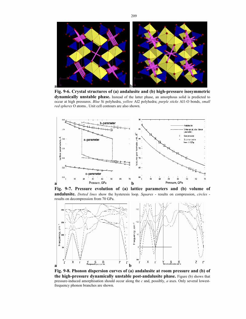
209
a b Fig. 9-6. Crystal structures of (a) andalusite and (b) high-pressure isosymmetric dynamically unstable phase. Instead of the latter phase, an amorphous solid is predicted to occur at high pressures. Blue Si polyhedra, yellow Al2 polyhedra; purple sticks Al1-O bonds, small red spheres O atoms.. Unit cell contours are also shown.
a b Fig. 9-7. Pressure evolution of (a) lattice parameters and (b) volume of andalusite. Dotted lines show the hysteresis loop. Squares - results on compression, circles - results on decompression from 70 GPa.
a b Fig. 9-8. Phonon dispersion curves of (a) andalusite at room pressure and (b) of the high-pressure dynamically unstable post-andalusite phase. Figure (b) shows that pressure-induced amorphisation should occur along the c and, possibly, a axes. Only several lowest-frequency phonon branches are shown.
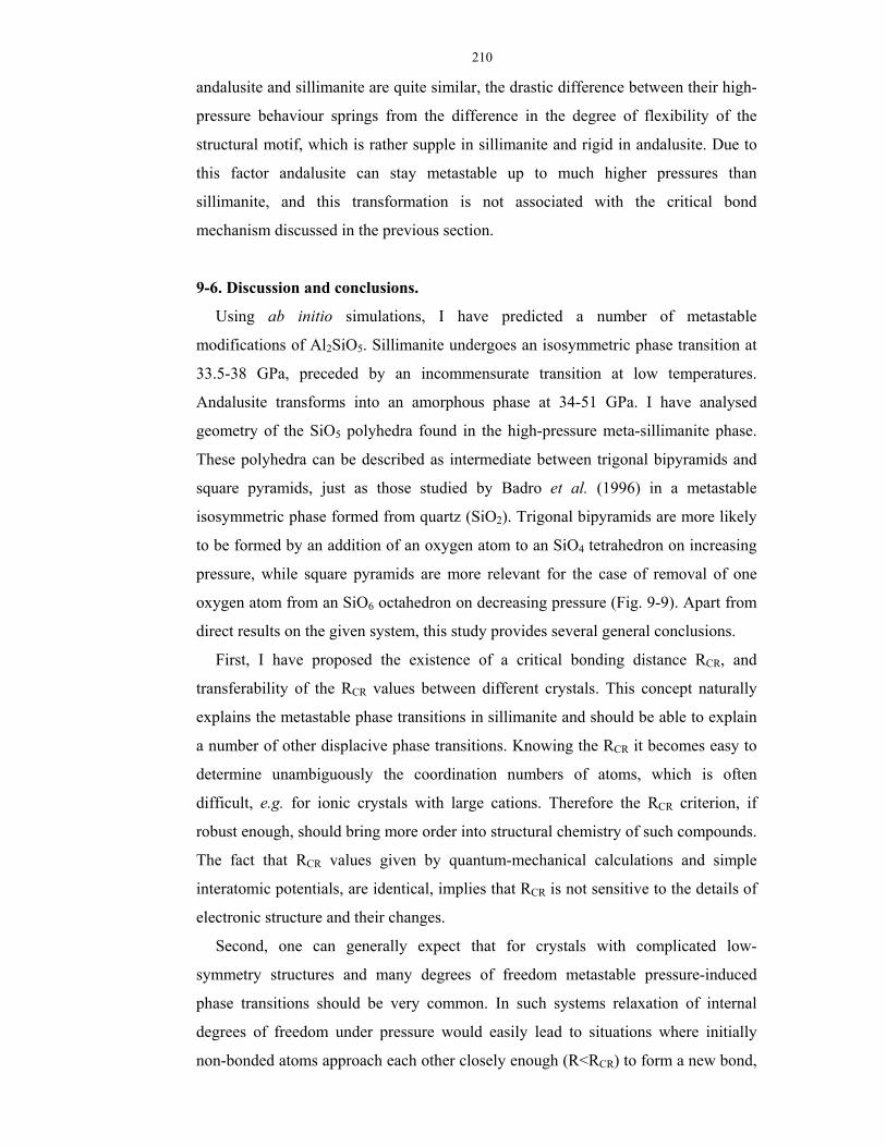
210
andalusite and sillimanite are quite similar, the drastic difference between their high-
pressure behaviour springs from the difference in the degree of flexibility of the
structural motif, which is rather supple in sillimanite and rigid in andalusite. Due to
this factor andalusite can stay metastable up to much higher pressures than
sillimanite, and this transformation is not associated with the critical bond
mechanism discussed in the previous section.
9-6. Discussion and conclusions.
Using ab initio simulations, I have predicted a number of metastable
modifications of Al2SiO5. Sillimanite undergoes an isosymmetric phase transition at
33.5-38 GPa, preceded by an incommensurate transition at low temperatures.
Andalusite transforms into an amorphous phase at 34-51 GPa. I have analysed
geometry of the SiO5 polyhedra found in the high-pressure meta-sillimanite phase.
These polyhedra can be described as intermediate between trigonal bipyramids and
square pyramids, just as those studied by Badro et al. (1996) in a metastable
isosymmetric phase formed from quartz (SiO2). Trigonal bipyramids are more likely
to be formed by an addition of an oxygen atom to an SiO4 tetrahedron on increasing
pressure, while square pyramids are more relevant for the case of removal of one
oxygen atom from an SiO6 octahedron on decreasing pressure (Fig. 9-9). Apart from
direct results on the given system, this study provides several general conclusions.
First, I have proposed the existence of a critical bonding distance RCR, and
transferability of the RCR values between different crystals. This concept naturally
explains the metastable phase transitions in sillimanite and should be able to explain
a number of other displacive phase transitions. Knowing the RCR it becomes easy to
determine unambiguously the coordination numbers of atoms, which is often
difficult, e.g. for ionic crystals with large cations. Therefore the RCR criterion, if
robust enough, should bring more order into structural chemistry of such compounds.
The fact that RCR values given by quantum-mechanical calculations and simple
interatomic potentials, are identical, implies that RCR is not sensitive to the details of
electronic structure and their changes.
Second, one can generally expect that for crystals with complicated low-
symmetry structures and many degrees of freedom metastable pressure-induced
phase transitions should be very common. In such systems relaxation of internal
degrees of freedom under pressure would easily lead to situations where initially
non-bonded atoms approach each other closely enough (R<RCR) to form a new bond,

211
which automatically triggers a phase transition. There are several systems in which
such transitions are very likely – titanite-like CaSi2O5, SiO2 (quartz and coesite),
feldspars, zeolites, berlinite AlPO4.
A B
C D
E Fig. 9-9. Genesis of the fivefold coordination of silicon. Tetrahedral Si (A) can capture a neighbouring O atom (B), becoming fivefold-coordinate (C). The coordination polyhedron is intermediate between trigonal bipyramid and square pyramid (cf. Fig. 3), into which it can easily transform by Berry pseudorotation (C→D). Capturing another O atom, a square bipyramid becomes an octahedron (D, E). The reverse transformation path is equally possible. In this study we see stages A-C; Angel et al. (1996) and Warren et al. (1999) observed stages D-E in CaSi2O5.
As structures tend to accommodate minimum changes necessary to maintain
stability, symmetry will be preserved whenever possible. The predicted transitions
are certainly local in the terminology of Chapter 4, but the cases of sillimanite and
andalusite are opposite extremes in the sense that the high-pressure transition in
sillimanite preserves all symmetry, while the transition in andalusite completely
destroys crystal symmetry.
212
Chapter 10. Thermoelasticity and phase
transitions of MgSiO3 perovskite.
MgSiO3 perovskite is the most abundant mineral in the Earth’s lower mantle and
in the Earth generally. The experimental information on many of its properties is
discrepant; some of the properties (e.g., elastic constants at high pressures and
temperatures) have not been measured at all. Ab initio simulations can resolve the
existing controversies and often give reliable predictions of the properties that cannot
currently be studied in the laboratory. Such simulations have been performed; their
results have significantly extended the current understanding of the Earth’s mantle.
The results presented in this chapter have been published in three papers (Oganov et
al., 2000; Oganov et al., 2001a,b). In the following discussion, I shall highlight such
issues relevant to the mantle as its composition, temperature distribution, mantle
convection, nature of the electrical conductivity of the lower mantle, and the
possibility of partial melting of the mantle.
10.1. Introduction.
It is established, by the analysis of phase diagrams (Ringwood, 1991) and mantle
inclusions in diamonds (Harte et al., 1999), that MgSiO3 perovskite48 (Mg-pv) is the
main mineral of the Earth’s lower mantle (at least 60 vol.%) and the most abundant
mineral in the Earth. Yet, there are major controversies in the experimental
information on many of its important properties.
The EOS of this phase at simultaneously high pressures and temperatures of the
lower mantle (pressure between 24 and 136 GPa, temperature ca 2000-3000 K) is
crucial for interpreting seismological data and constructing reliable chemical,
mineralogical, and thermal models of the lower mantle. Yet, accurate experimental
48 Of course, not pure. In the lower mantle, it is generally expected to have the composition close to
(Mg0.9Fe0.1)SiO3, probably with a few percent Al2O3. The effects of the moderate Fe content, while
potentially important for certain properties (e.g., shear modulus), are expected to be negligible for
others, especially for the thermal expansion, bulk modulus, and p-T-derivatives of the elastic moduli
and seismic wave velocities. For this reason, most experimental and theoretical studies concentrate on
the pure Mg-pv. Recent ab initio study by Brodholt (2000) showed that Al impurities would
significantly affect the EOS of Mg-pv only below ~30 GPa.

213
EOS of Mg-pv is available only at 298 K (e.g., Knittle & Jeanloz 1987; Fiquet et al.
2000). Accurate experimental measurement of the temperature effects still poses a
problem – e.g., there is a sharp conflict between different experimental data on
thermal expansion coefficient of Mg-pv. At the same time, thermal expansion of Mg-
pv, crucial for models of the lower mantle composition and dynamics, is poorly
known even at the ambient conditions (for a discussion see Anderson et al., 1995;
Ringwood, 1991). For the Grüneisen parameter γ0, the reported values at ambient
conditions are scattered between 1.2 and 2.0, and its volume dependence parameter,
q=∂lnγ/∂lnV, is uncertain roughly between 1 and 2.5. The difficulties in obtaining
accurate thermoelastic parameters of this mineral from experiment were discussed in
detail by Shim and Duffy (2000).
The highest experimentally reached hydrostatic pressure in experiments at the
lower mantle temperatures is 94 GPa (Fiquet et al., 2000), which is still well below
the core-mantle boundary pressure of 136 GPa. Moreover, experiments at such high
pressures and high temperatures can presently be performed only in laser-heated
diamond anvil cells with very large uncertainties in temperature. To reproduce the
extreme conditions of the lower mantle remains a major challenge for both
theoreticians working at the ab initio level and experimentalists.
The elastic constants have been studied experimentally only at ambient conditions
(Yeganeh-Haeri, 1994). One needs to know these constants at the lower mantle
pressures and temperatures in order to be able to interpret seismic tomography maps
in terms of the temperature distribution (see Oganov et al., 2001b and below).
These and other issues can now be addressed with accurate ab initio simulations.
A breakthrough in theoretical simulations was marked by the works of Stixrude and
Cohen (1993) and Wentzcovitch et al. (1993), who demonstrated the feasibility and
enormous potential of quantum-mechanical simulations based on density functional
theory. In parallel with these studies, D’Arco et al. (1993) performed successful
Hartree-Fock simulations of this mineral. A number of important contributions have
been made since (D’Arco et al., 1994; Wentzcovitch et al., 1995, 1998; Karki et al.,
1997, 2000, 2001; Warren et al., 1998; Brodholt, 2000; Oganov et al., 2000,
2001a,b).

214
10.2. Computational methodology.
Ab initio. All my ab initio simulations of Mg-pv (Oganov et al., 2001a,b and this
work) are based on DFT and use the PW91 GGA (Wang & Perdew, 1991; see
Chapter 5). Plane wave pseudopotential methodology as implemented in the VASP
code (Kresse & Furthmüller, 1996a,b) is used. I use very accurate non-local
pseudopotentials for all atoms; for O atoms an ultrasoft pseudopotential (Vanderbilt,
1990) was used49. The ground state was found by solving the Kohn-Sham equations
self-consistently to within 5*10-10 eV/atom; static structure was optimised to within
5*10-10 eV/atom using the conjugate gradients method. For the Brillouin zone
sampling I used 2*2*2 meshes for the orthorhombic (space group Pbnm) and
tetragonal I4/mcm-phases (each having 20 atoms in the conventional unit cell) and
4*4*4 mesh for the cubic (Pm−3m) phase. This proved to be sufficient for an accurate
determination of the equations of state, elastic constants, and the enthalpy
differences.
The use of an ultrasoft pseudopotential for oxygen allowed me to use a relatively
small basis set with the plane-wave cut-off energy of 500 eV without any loss of
accuracy and perfect convergence of all properties with respect to the basis set size
(the Pulay stress was only 0.05 GPa and was neglected). This significantly reduced
the computational cost of the simulations, allowing me to perform the largest-scale
ab initio molecular dynamics simulations of this mineral up-to-date (Oganov et al.,
2001a,b) and address such challenging issues as elasticity at high pressures and
temperatures of the lower mantle (Oganov et al., 2001b). Such issues cannot
presently be addressed by experiments.
Our work (Oganov et al., 2001b) has reported, to the best of our knowledge, the
first finite-temperature calculations of the elastic constants of any material using ab
initio molecular dynamics (MD). These dynamical simulations were performed in the
constant-temperature (NVT) ensemble (Nosé, 1984) with an 80-atom supercell
(2a*2b*1c Pbnm-supercell), Γ-point for the Brillouin-zone sampling, and a timestep
of 1 fs; for each configuration the ground state was found self-consistently to within
6.25*10-8 eV/atom. The dynamical simulations were run for at least 0.8 ps after
equilibration. The thermostat mass parameter was optimised so as to produce
49 The pseudopotentials for Mg and Si are norm-conserving (Rappe et al., 1990) with partial core
corrections (Louie et al., 1982). The core radii are 1.06 Å for Mg (valence configuration 3s23p03d0),
0.95 Å for Si (3s23p23d0), and 0.82 Å for O (2s22p43d0).
215
temperature oscillations with a period of atomic vibrations. Our ab initio MD runs,
although relatively short, proved to be sufficient for obtaining well-converged
statistical averages for the stress tensor. All calculations were performed on the
CRAY T3E supercomputer at Manchester Computer Centre.
The elastic constants were calculated, following Karki (1997) and the theory
outlined in Chapter 3, from the non-linear stress-strain relations using simulations at
a series of small strains (0, 1%, 2%, and 3%) and fitting the stress-strain functions
with 2nd order polynomials. It is essential to consider the non-linear elastic effects in
such calculations. In my ab initio MD simulations, I used +2% and –2% strains; the
use of two independent MD calculations, apart from accounting for the non-linear
effects, significantly increased the statistical significance of the results.
Most of the previous workers (Wentzcovitch et al., 1993, 1995; Karki et al., 1997,
2000, 2001; Warren et al., 1998) utilised the local density approximation (LDA) of
density functional theory and hard pseudopotentials; Stixrude and Cohen (1993) used
LDA in conjunction with all-electron LAPW method. D’Arco et al. (1993, 1994)
used Hartree-Fock method. Currently, GGA is the state-of the art in quantum-
mechanical computational studies, but an encouraging circumstance is that results of
the GGA, LDA, and Hartree-Fock calculations are in a good semiquantitative
agreement with each other for Mg-pv, as well as for many other ionic systems.
Results of different ab initio methods are compared in Table 10-1. HF calculations
are very accurate in describing its crystal structure, but not elasticity or binding
energy. LDA and GGA are capable of giving high accuracy for the prediction of the
crystal structure as well as its response to pressure and temperature.
The GGA systematically overestimates bond lengths and unit cell parameters by
~1-2%. This causes significant errors in the EOS. In a recent comparative study
(Favot & Dal Corso, 1999) of the GGA- and LDA- phonon dispersion curves in
several compounds it was suggested that the gradient corrections to the LDA act as a
negative pressure. Usually, GGA overcorrects the LDA, resulting in overexpansion
of crystal structures and lowering of the vibrational frequencies and elastic moduli50.
An important observation is that this error can be largely ascribed to an error in the 50 The nature of this effect was discussed in Chapter 5. In most cases, GGA overexpands crystal
structures because the gradient corrections favour more inhomogeneous electron density distribution
achieved in more open structures. Patton et al. (1997) arrived at the same conclusion. Oganov and
Brodholt (2000) suggested that for the same reason lower-density phases are often more energetically
favourable in the GGA than in the LDA or in experiment.

216
pressure: GGA can be imagined to contain some spurious pressure, which shifts the
whole pressure scale by a constant51, while leaving all properties as a function of
volume unchanged. Indeed, for Mg-pv, GGA calculations (see Table 10-1 and below)
at the experimental unit cell volume at ambient conditions (162.40 Å3) give all the
elastic constants coinciding with the experimental values within the experimental
errors. In these calculations, all the lattice parameters and atomic positions were fully
relaxed under the only constraint of a fixed unit cell volume. The GGA volume
dependences of the elastic constants are in excellent agreement with independent
LDA simulations of Karki et al. (1997) (see Fig. 10-1).
The systematic error of the GGA can be systematically corrected by shifting the
GGA pressures by a constant, effectively recovering the experimental unit cell
volume at ambient conditions (see Oganov et al., 2001a). A similar procedure was
used by Vanderbilt (1998) in his LDA studies of phased transitions in perovskites.
This simple procedure, although not fully ab initio, is useful because it allows one to
obtain very accurate results for the elastic constants and EOS of Mg-pv and gives
confidence in the simulated thermal properties.
The pressure correction is easy to work out. Writing the corrected pressure as
follows:
p truetotal (V,T) = p GGA
st (V) + pth(V,T) + ∆p , (10.2.1)
for the volume corresponding to the ambient conditions (where p truetotal = 0) we have
the pressure correction:
∆p = -p GGAst (V0) - pth(V0,T) (10.2.2)
The first term is just minus the GGA static pressure at the experimental volume (-8.5
GPa) and the second term is minus the thermal pressure at this volume and 298 K (-
3.58 GPa). The second term was evaluated using the Grüneisen parameter from ab
initio MD simulations (see below). Pressure-corrected GGA turns out to be far more
accurate than any other ab intio method in Table 10-1. In what follows, pressure
correction was not applied only in the calculations of the relative stability of different
Table 10-1. Ab initio simulations of MgSiO3 perovskite. HF results are from D’Arco et al. (1993, 1994); GGA results are from Oganov et al. (2001a). ‘GGA+p’ means pressure-corrected GGA. Propert HF LDA GGA GGA+p Exp.
51 Note that a constant pressure correction is equivalent to adding an energy term linear in volume. At
each volume, this leaves unchanged all properties that are second or higher derivatives of the energy.

217
y a b c V0, Å3 162.12 157.50 162.47 157.87 168.04 162.40 162.45 a0, Å 4.786 4.711 4.7891 4.7272 4.8337 4.7765 4.7747 b0, Å 4.913 4.880 4.9219 4.8889 4.9830 4.9333 4.9319 c0, Å 6.896 6.851 6.8925 6.8311 6.9767 6.8919 6.8987
Mg xyz
0.5112 0.5476 ¼
0.5174 0.5614 ¼
0.5129
0.5521
¼
0.5160 0.5576 ¼
0.5148 0.5552 ¼
0.5154 0.5570 ¼
0.5143 0.5556 ¼
Si (x; y; z) (0; ½; 0) (0; ½; 0) (0; ½; 0) (0; ½; 0) (0; ½; 0) (0; ½; 0) (0; ½; 0) O1 x
yz
0.0999 0.4643 ¼
0.1128 0.4608 ¼
0.0980 0.4686
¼
0.1044 0.4654 ¼
0.1018 0.4664 ¼
0.1030 0.4666 ¼
0.1037 0.4655 ¼
O2 xy z
0.1980 0.2029 0.5522
0.1928 0.1995 0.5582
0.1983 0.2033 0.5507
0.1969 0.2015 0.5539
0.1983 0.2031 0.5527
0.1972 0.2019 0.5530
0.1974 0.2011 0.5538
C11, GPa - 496 487 499 444 493 482 C22 - 560 524 561 489 546 537 C33 - 504 456 466 408 470 485 C12 - 132 128 123 110 142 144 C13 - 136 144 137 126 146 147 C23 - 156 156 142 136 160 146 C44 - 151 203 217 194 212 204 C55 - 198 186 186 172 186 186 C66 - 171 145 160 131 149 147 KV, GPa - 267.6 258.1 258.8 231.7 267.2 264.2 KR 309 266.5 257.5 257.8 230.9 266.2 263.7 KVRH - 267.1 257.8 258.3 231.3 266.7 264.0 GV, GPa - 179.7 176.1 187.6 164.0 180.1 178.5 GR - 177.8 173.3 185.1 160.5 177.4 176.2 GVRH - 178.7 174.7 186.3 162.3 178.7 177.4 CL, m/s - 10926 10935 10953 10620 11091 11042 CT - 6498 6524 6641 6395 6598 6574 θD, K - 1077 1069 1097 1036 1082 1078
a – Wentzcovitch et al. (1995) b – Karki et al. (1997); Karki (1997)
c – This work. The same computational parameters were used as in the GGA simulations. All pseudopotentials used in LDA-simulations were generated within the LDA. LDA-pseudopotential for Si was of the same type as the one used in GGA-simulations, with the same valence configuration, core radius, and also with partial core corrections. LDA-pseudopotential for Mg was ultrasoft with valence configuration 2p63s23d0, core radius 1.06 Å, and partial core corrections. Pseudopotential for O was ultrasoft with valence configuration 2s22p43d0 and core radius 1.01 Å. The results are much closer to those of Wentzcovitch et al. (1995) than to those of Karki et al. (1997).
d – Crystal structure from (Ross & Hazen, 1989). Elastic constants and related properties from (Yeganeh-Haeri, 1994) or calculated using data of Yeganeh-Haeri (1994).
perovskite polymorphs. The large energy differences obtained in such calculations
should be sufficiently accurate, especially because the (already small) energy terms
related to the pressure correction largely cancel in calculations of the energy
differences.
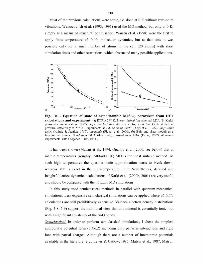
218
Most of the previous calculations were static, i.e. done at 0 K without zero-point
vibrations. Wentzcovitch et al. (1993, 1995) used the MD method, but only at 0 K,
simply as a means of structural optimisation. Warren et al. (1998) were the first to
apply finite-temperature ab initio molecular dynamics, but at that time it was
possible only for a small number of atoms in the cell (20 atoms) with short
simulation times and other restrictions, which obstructed many possible applications.
a b
Fig. 10-1. Equation of state of orthorhombic MgSiO3 perovskite from DFT calculations and experiment. (a) EOS at 298 K. Lower dashed line athermal LDA (B. Karki, personal communication, 1997), upper dashed line athermal GGA, solid line GGA shifted in pressure, effectively at 298 K. Experiments at 298 K: small circles (Yagi et al., 1982), large solid cirles (Knittle & Jeanloz, 1987), diamonds (Fiquet e al., 2000). (b) Bulk and shear moduli as a function of volume. Solid lines GGA (this study); dashed lines LDA (Karki, 1997), diamonds experimental data (Yeganeh-Haeri, 1994).
It has been shown (Matsui et al., 1994, Oganov et al., 2000, see below) that at
mantle temperatures (roughly 1500-4000 K) MD is the most suitable method. At
such high temperatures the quasiharmonic approximation starts to break down,
whereas MD is exact in the high-temperature limit. Nevertheless, detailed and
insightful lattice-dynamical calculations of Karki et al. (2000b, 2001) are very useful
and should be compared with the ab initio MD simulations.
In this study used semiclassical methods in parallel with quantum-mechanical
simulations. Less expensive semiclassical simulations can be applied where ab initio
calculations are still prohibitively expensive. Valence electron density distributions
(Fig. 5-8, 5-9) support the traditional view that this mineral is essentially ionic, but
with a significant covalency of the Si-O bonds.
Semiclassical. In order to perform semiclassical simulations, I chose the simplest
appropriate potential form (5.3.6.2) including only pairwise interactions and rigid
ions with partial charges. Although there are a number of interatomic potentials
available in the literature (e.g., Lewis & Catlow, 1985; Matsui et al., 1987; Matsui,

219
1988; Wall, 1988; Leinenweber & Navrotski, 1988; Choudhury et al., 1988; Kubicki
& Lasaga, 1991; Ghose at al., 1992; Stuart & Price, 1996), I preferred to derive my
own potential.
First of all, many previous potentials were derived from fitting calculated
structure and properties at T = 0 K to experimental data at 300 K. Recent
developments in the GULP code (Gale, 1996, 1997, 1998), which I used in my work
(Oganov et al., 2000), for the first time allowed us to include quasiharmonically all
thermal and zero-point motion effects in the fitting procedure, which itself now
involves complete structure optimisation for each set of trial potential parameters,
making the whole procedure much more rigorous. Implementation of analytical free
energy derivatives (Kantorovich, 1995; Gale, 1998) has speeded up free energy
minimisation by orders of magnitude, thus enabling finite-temperature fitting even
for relatively large systems.
Some previous potentials, e.g. purely ionic transferable potential models (Lewis &
Catlow, 1985), are known to perform poorly for Mg-pv. This can clearly be improved
by adopting partial ionic charges (e.g., Matsui, 1988).
Another problem is that none of the previous studies paid any attention to the
severe correlation problem between the potential parameters (e.g., ρij and bij in
(5.3.6.2)) in the potential, leading to poor transferability and reliability of the
potential for the prediction of properties not used in fitting. Statistical significance of
the fitted potential parameters is often poor, because the number of observables used
in fitting is usually comparable to the number of the fitted parameters. These
problems can be solved by setting some of the parameters to values, determined by
physical considerations. I fixed ρij at the values, calculated from (5.3.6.3). This
physical determination of the repulsion exponents ρij ensures the best transferability
of such a potential, and removes the problem of correlation between bij and ρij. The
O-O short-range potential (bO-O = 2023.8 eV, ρO-O = 0.2674 Å and cO-O = 13.83
eV*Å6) was taken from Gavezzotti’s works (e.g., 1994), where it was extensively
validated for organic compounds. Oxygen-oxygen short-range potential is very weak
in most existing models, and therefore its details are not very important. I preferred
Gavezzotti’s potential, because it had the closest ρij to the one given by (5.3.6.3) and
a reasonable van der Waals parameter cO-O.
I neglected weak cation-cation short-range interactions and cation-anion
dispersion interactions. As a result, only 4 independent parameters had to be fitted:
220
atomic charges ZSi and ZMg (ZO=-1/3(ZMg+ZSi)), and pre-exponential repulsive
parameters bMg-O, and bSi-O. These parameters are virtually uncorrelated with each
other and give a stable solution for the fitting problem. In this fitting procedure, I
used experimental crystal structure at 1 atm and 300 K (Ross & Hazen, 1989) and
full elastic constants tensor (Yeganeh-Haeri, 1994). Temperature was explicitly
included via quasiharmonic LD treatment with analytical free energy derivatives. A
2*2*2 grid was used for the Brillouin zone sampling in this finite-temperature fitting.
The resulting potential parameters are: ZMg = +1.9104; ZSi = +2.9043; ZO = -
1.6049; bMg-O =1007.526 eV, ρMg-O = 0.2866Å; bSi-O = 1108.983 eV, ρSi-O = 0.2827Å;
bO-O = 2023.8 eV, ρO-O = 0.2674 Å, cO-O = 13.83 eV*Å6. Note that a simple crystal
potential fitting procedure has given chemically reasonable atomic charges. Results
obtained with this potential are given in Table 10-2. One can see that apart from
describing well crystal structure and elastic properties, this potential gives very
reasonable thermal expansion coefficient, which was not used in the fitting of the
potential. The calculated shear modulus is underestimated; this is partly responsible
for the small overestimation of the entropy (Table 10-2). The calculated heat
capacity and entropy at 300 K compare well with experimental estimates and are
superior to those calculated with previous potentials (Stuart & Price, 1996). Room-
temperature Birch-Murnaghan EOS parameters are: K0=266 and 269 GPa, K’= 3.9
and 4.04 in experiment (Knittle & Jeanloz, 1987) and theory (my LD calculations),
respectively. These observations strongly support this simple potential, which
perhaps is as good as a pairwise rigid-ion model can be.
This interatomic potential has been used (Oganov et al., 2000) in a comparative
study of LD and MD simulations, as well as of the Debye model, applied to Mg-pv.
The results of that study are presented in the next section.
10.3. Comparative study of LD, MD and Debye model applied to MgSiO3
perovskite.
Debye model (DM). It has become an almost common practice (e.g., Stixrude et
al., 1992; Anderson et al., 1995; Jackson & Rigden, 1996; Yagi & Funamori, 1996;
Shim & Duffy, 2000; Stacey & Isaak, 2000; Hama et al., 2000) to use the Debye
model (DM) in geophysical studies, in fitting the experimental thermal expansion,
heat capacity data, or experimental equations of state. The DM does describe the
shape of the temperature dependences of thermodynamic functions of solids, and this

221
is the reason why it often can be used for their fitting even without Debye theory
being quantitatively accurate or even physically realistic. Anderson (1998) claimed
Table 10-2. Performance of the fitted interatomic potential: crystal structure and elastic properties of MgSiO3 perovskite. Elastic properties in GPa, α in 10-5 K-1, CV and S are in J/(mol*K).
Property Rigid-ion model (Oganov et al., 2000)
Experiment
a0, Å 4.7822 4.7747 b0, Å 4.8960 4.9319 c0, Å 6.9322 6.8987 V0, Å3 162.31 162.45
Mg (x; y; z) (0.5056; 0.5267; ¼) (0.5143; 0.5556; ¼) Si (x; y; z) (0; ½; 0) (0; ½; 0) O1 (x; y; z) (0.1026; 0.4620; ¼) (0.1037; 0.4655; ¼) O2 (x; y; z) (0.1982; 0.2014; 0.5526) (0.1974; 0.2011; 0.5538)
C11 500 482 C22 509 537 C33 398 485 C12 116 144 C13 210 147 C23 188 146 C44 174 204 C55 189 186 C66 102 147 KVRH 270.4 264.0 GVRH 146.3 177.4 θD, K 984 1078 α 2.09 1.57a; 2.2b CV 80.88 80.6c
S 61.81 57.2c a – Fiquet et al. (1998). b – Ross et al. (1989). Experimental data on the volume thermal expansion coefficient of MgSiO3
perovskite are still highly uncertain. The most plausible range is 1.5-1.9*10-5 K-1 at 300 K and 1 atm. c –Cp and S from Akaogi and Ito (1993).
that ‘MgSiO3-perovskite is one of a small, select group of Debye-like minerals, for
which thermoelastic properties and the equation of state (EOS) are calculable from
acoustic data’.
In the Mie-Grüneisen formalism (see Chapter 3), all one needs to know to
construct a high-temperature EOS is a reference isothermal (e.g., static) EOS and
functions CV(V,T) and γ(V). It is possible to obtain both CV and γ using lattice-
dynamical models, of which the DM is the simplest. This model has been considered
in Chapter 3. Here I only need to add that in this model there is a simple
quasiharmonic expression for the Grüneisen parameter:
222
γ = - Vd
d D
lnlnθ
, (10.3.1)
From the computational point of view this model is very tempting, since using
only static EOS and elastic constants this model allows one to predict all
thermoelastic properties at arbitrary p-T-conditions. Accurate ab initio static EOS
and elastic constants of Mg-pv already exist in the literature (Wentzcovitch et al
1995, 1998; Karki et al. 1997; Oganov et al., 2001a).
Thoroughly reviewed and criticised as inapplicable to most minerals (Kieffer,
1979a), the DM in application to MgSiO3 perovskite was rehabilitated by O.L.
Anderson (1998), who has shown that it yields very accurate values of CV at ambient
pressure and T>400 K.
However, it has never been demonstrated that (10.3.1) does give accurate results.
In fact, it does not, as I show below. Recently, Stacey and Isaak (2000) used acoustic
Grüneisen parameters to construct EOS of the lower mantle minerals. Hama et al.
(2000) used a self-consistent DM in order to obtain thermal EOS and seismic
velocities of the major lower mantle minerals and construct a mineralogical and
thermal model of the lower mantle. Since (10.3.1) is not accurate, such an approach
is very crude.
What is a Debye-like solid? There are no strictly Debye-like solids, i.e. solids
satisfying all the assumptions of Debye theory. With regards to geophysical
applications, high-p-T EOS, elastic properties, and thermal expansion are the key
quantities of interest, and therefore for a Debye-like solid the DM should closely
reproduce 1. heat capacity CV(T), at least at elevated temperatures, and
2. Grüneisen parameter γ(V).
Errors in any of these quantities will result in erroneous thermal EOS and,
therefore, invalidate the model. For DM to give a reasonable CV(T), Anderson (1998)
formulated the following conditions: a) no gap should be present in the phonon
spectrum, b) not many modes should have frequencies above the maximum Debye
frequency, kθD/h , c) phonon density of states should be close to (3.3.1) at least in
the limit of small ω. One can see (Fig. 10-2) that conditions a-c are met for Mg-pv.
This explains why Debye theory gives accurate predictions for CV(T). Nevertheless,
as I show below, Mg-pv is not a Debye-like solid, since DM does not give accurate
predictions for its γ(V). Part of the reason is that in structures of such level of

223
complexity, optic modes (whose behaviour is not directly linked to the elastic
constants) dominate. This and some other important conclusions have been reached
by comparing the results of the self-consistent DM (based on the calculated athermal
EOS and elastic constants) with more accurate LD and MD simulations based on the
same model interatomic potential.
Unlike the DM, the LD and MD calculations take into account all the phonons
across the Brillouin zone and not just the acoustic modes at k→0, and intrinsic
anharmonic effects are also accounted for by MD simulations. As we shall see, the
DM does not reproduce the full-phonon calculations.
a b
Fig. 10-2. Phonon density of states (DOS) of MgSiO3 perovskite. (a) Full harmonic calculation versus the Debye model. (b) Projections of the total harmonic DOS onto atomic species. Athermal calculations at 0 GPa (V0=160.46 Å3). For a Debye solid, all atoms have a constant proportion of the total DOS determined by relative masses and numbers of atoms of each sort. LD-calculations show that this is far from reality: Mg-contribution clearly tends to the low-frequency part, while Si-projection leans to the high-frequency region of the DOS, as a direct result of the different bond strengths (Si-O bonds are much stiffer than Mg-O).
Computational methodology. LD calculations were performed with GULP, using
analytical free energy derivatives and without the commonly used ‘ZSISA’ (see
Chapter 5). Free energy minimisation was performed with 6*6*6 grids for the
Brillouin zone integration. This grid showed very good convergence for all
properties. For calculations of the density of states and its projections and heat
capacity (CV) I used even denser grids – 12*12*12 and 20*20*20, respectively.
MD calculations were performed with the Moldy code (Refson 1988-2000). The
NPT-ensemble in conjunction with Nose-Hoover (Hoover, 1985) thermostat and
Parrinello-Rahman (Parrinello & Rahman, 1981) constant-pressure algorithm was
used throughout. The computational box contained 540 atoms (3*3*3 supercell),
which was sufficient to obtain highly accurate results. The system was allowed to
evolve for 10 ps, of which the first 5 ps were used for equilibration and not included
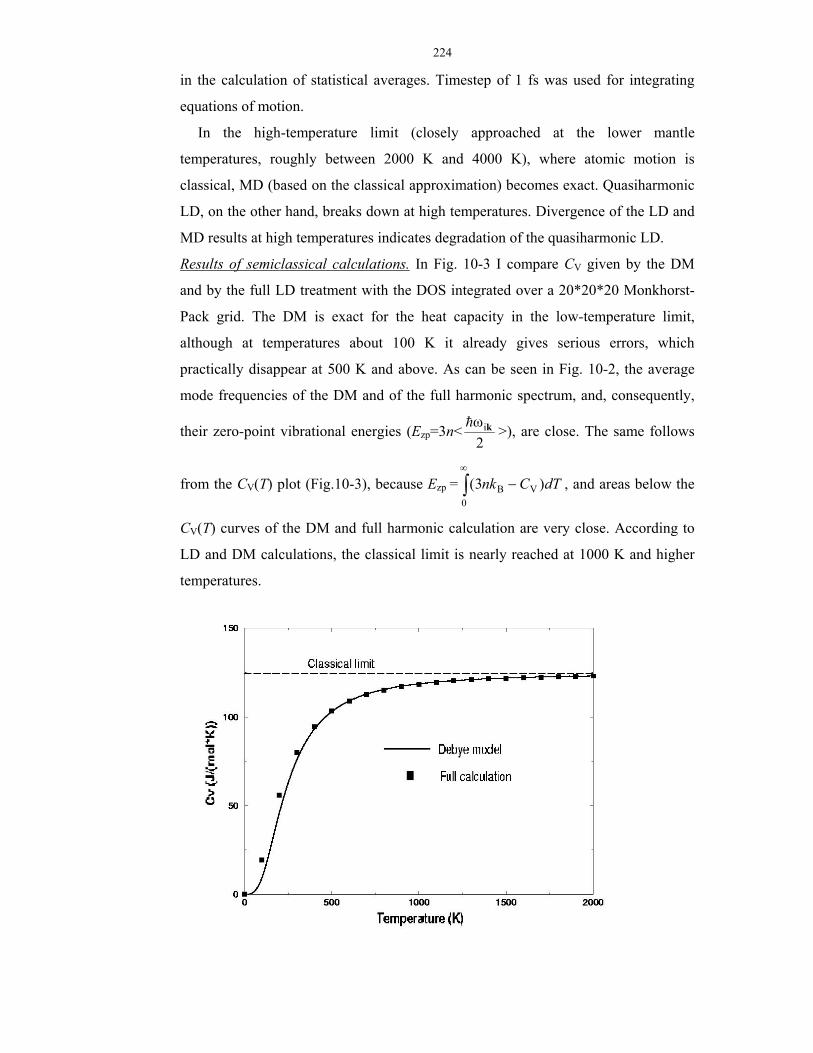
224
in the calculation of statistical averages. Timestep of 1 fs was used for integrating
equations of motion.
In the high-temperature limit (closely approached at the lower mantle
temperatures, roughly between 2000 K and 4000 K), where atomic motion is
classical, MD (based on the classical approximation) becomes exact. Quasiharmonic
LD, on the other hand, breaks down at high temperatures. Divergence of the LD and
MD results at high temperatures indicates degradation of the quasiharmonic LD.
Results of semiclassical calculations. In Fig. 10-3 I compare CV given by the DM
and by the full LD treatment with the DOS integrated over a 20*20*20 Monkhorst-
Pack grid. The DM is exact for the heat capacity in the low-temperature limit,
although at temperatures about 100 K it already gives serious errors, which
practically disappear at 500 K and above. As can be seen in Fig. 10-2, the average
mode frequencies of the DM and of the full harmonic spectrum, and, consequently,
their zero-point vibrational energies (Ezp=3n<2ωikh >), are close. The same follows
from the CV(T) plot (Fig.10-3), because Ezp = ∫∞
−0
VB )3( dTCnk , and areas below the
CV(T) curves of the DM and full harmonic calculation are very close. According to
LD and DM calculations, the classical limit is nearly reached at 1000 K and higher
temperatures.

225
Fig. 10-3. Heat capacity CV of MgSiO3 perovskite. Filled squares - harmonic calculation, solid line - Debye model. The calculations were done at the volume corresponding to 0 GPa and athermal conditions (V0=160.46 Å3).
Fig. 10-4a depicts the temperature dependence of the Grüneisen parameter at 50
GPa. In LD and MD calculations the Grüneisen parameter was calculated from the
thermal expansion coefficient via eq. (3.7.5)52. The high-temperature constant value
(<γik> - see Chapter 3) is virtually reached in LD calculations at 500 K, and a small
linear increase of γ is due to the change of volume with temperature. MD, based on
the classical approximation, always gives the high-temperature limit value. Below
500 K, LD gives a noticeable non-monotonic temperature variation of γ. A sudden
rise and anomalously high values of γ, found in LD-calculations at T>2000 K, are
artifacts of the QHA and indicate its breakdown in this temperature range, where MD
is a more justified technique. DM does not reproduce neither LD nor MD results. A
similar picture is observed for the thermal expansion (Fig. 10-4b).
Fig. 10-5 shows the results of full-phonon calculations of the high-temperature γ
in comparison with the predictions of the DM. Results of LD-calculations differ
significantly from MD-results, especially at large volumes (low pressures), in line
with the earlier work by Matsui et al. (1994). This is because of the neglect of the
intrinsic anharmonic effects in the QHA. Errors of the DM are typically about –30%
at all volumes, and reach almost -50% at the bottom of the lower mantle. This
implies an error of typically 30% in the thermal expansion coefficient.
a b
52 Since MD is based on the classical approximation, CV was assumed to be equal to (3n-3)kB (per
supercell containing n atoms). The anharmonic contribution, by eq. (3.6.2), is expected to be a few
percent of (3n-3)kB at mantle temperatures (<4000 K).
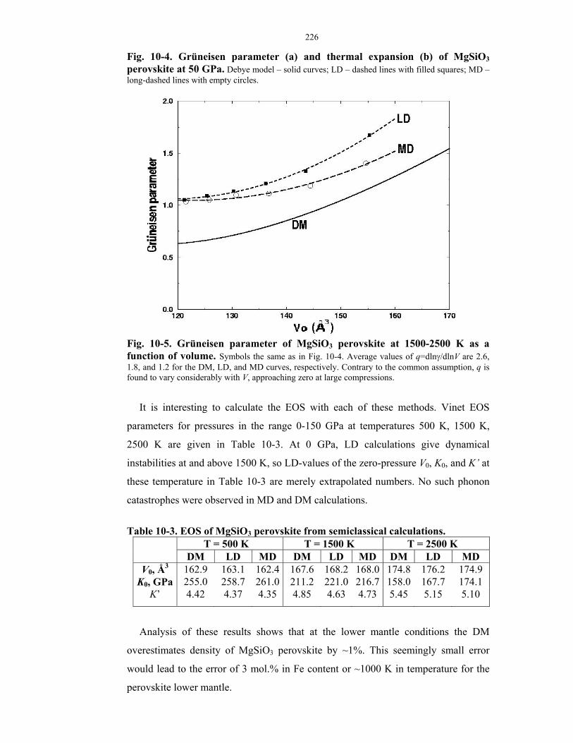
226
Fig. 10-4. Grüneisen parameter (a) and thermal expansion (b) of MgSiO3 perovskite at 50 GPa. Debye model – solid curves; LD – dashed lines with filled squares; MD – long-dashed lines with empty circles.
Fig. 10-5. Grüneisen parameter of MgSiO3 perovskite at 1500-2500 K as a function of volume. Symbols the same as in Fig. 10-4. Average values of q=dlnγ/dlnV are 2.6, 1.8, and 1.2 for the DM, LD, and MD curves, respectively. Contrary to the common assumption, q is found to vary considerably with V, approaching zero at large compressions.
It is interesting to calculate the EOS with each of these methods. Vinet EOS
parameters for pressures in the range 0-150 GPa at temperatures 500 K, 1500 K,
2500 K are given in Table 10-3. At 0 GPa, LD calculations give dynamical
instabilities at and above 1500 K, so LD-values of the zero-pressure V0, K0, and K’ at
these temperature in Table 10-3 are merely extrapolated numbers. No such phonon
catastrophes were observed in MD and DM calculations.
Table 10-3. EOS of MgSiO3 perovskite from semiclassical calculations.
T = 500 K T = 1500 K T = 2500 K DM LD MD DM LD MD DM LD MD
V0, Å3 162.9 163.1 162.4 167.6 168.2 168.0 174.8 176.2 174.9 K0, GPa 255.0 258.7 261.0 211.2 221.0 216.7 158.0 167.7 174.1
K’ 4.42 4.37 4.35 4.85 4.63 4.73 5.45 5.15 5.10
Analysis of these results shows that at the lower mantle conditions the DM
overestimates density of MgSiO3 perovskite by ~1%. This seemingly small error
would lead to the error of 3 mol.% in Fe content or ~1000 K in temperature for the
perovskite lower mantle.

227
Comparison of the experimental p(V)-isotherm at 2000 K and up to 90 GPa
(Fiquet et al., 1998, 2000) with the MD results shows the pressure difference up to 5
GPa, which is of the order of the experimental uncertainties. This again confirms the
validity of the model potential used.
Conclusions. The results just discussed indicate that Mg-pv cannot be regarded as a
good Debye-like solid, and its EOS cannot be accurately determined from acoustic
data, contrary to the conclusion of Anderson (1998). Adiabatic thermal gradient of
the lower mantle, (∂T/∂P)S=γT/KS, cannot be constructed without accurate
knowledge of the Grüneisen parameter γ. In agreement with this, Brown and
Shankland (1981) on the basis of Debye theory found an adiabatic temperature
increase of ~560 K across the lower mantle, while my ab initio adiabatic geotherm
(see below) gives much higher increase of ~800 K. When deriving the temperature
profile by matching PREM bulk modulus and density with the properties of plausible
mineral assemblages, errors of ~30% (i.e., ~1000 K) in the temperature would arise
from the use of acoustic γ.
If DM is used self-consistently (like in Hama et al. 2000), i.e. γ is related to the
volume derivatives of the acoustic velocities, significant errors are expected.
Likewise, it is not justified to extract γ from seismological profiles. On the other
hand, it should be safe to use the DM for inverting experimental data sets (e.g.,
Stixrude et al., 1992; Jackson & Rigden, 1996; Yagi & Funamori, 1996; Fiquet et al.,
2000; Shim & Duffy, 2000). However, in this case parameters of the model lose their
original meaning and become unrelated to the acoustic velocities.
It is now clear that at mantle temperatures only MD simulations can give very
accurate results. Such calculations will be discussed below, after I discuss an
important issue of the stability of Mg-pv in the lower mantle.
10.4. Stability of MgSiO3 perovskite.
If Mg-pv perovskite undergoes a phase transition within the lower mantle, it
would have dramatic consequences, at least by creating a major seismic boundary.
Indeed, there are seismic discontinuities in the lower mantle (e.g., Le Stunff et al.,
1995), but all of them are rather weak and may not be global.
Two main possibilities of a phase transition have been considered – 1)
temperature-induced transition to another perovskite phase and 2) breakdown of Mg-
pv into the mixture of oxides, MgSiO3→ MgO+SiO2. Both possibilities have been

228
reviewed in Chapter 2. There is almost no doubt that Mg-pv remains stable at mantle
conditions. The main question therefore is whether it remains in the usual
orthorhombic (Pbnm) phase or transforms into another perovskite phase at high
mantle temperatures.
The raison d’etre of any temperature-induced transition is the higher entropy of
the high-temperature phase; usually this means an increase of symmetry by means of
static or dynamic disorder. The cubic (Pm−3m) and tetragonal (I4/mcm) phases have
become the main (but not the only) candidates for the high-T phase. Together with
Pbnm, these are among the phases most commonly found in analogue perovskites.
The cubic phase should be a superionic conductor of electricity (O’Keeffe &
Bovin, 1979; Matsui & Price, 1991) due to the diffusion of O2- ions. Indeed,
geophysical observations and laboratory experiments show that the electrical
conductivity of the lower mantle is unusually high, ~1-10 S/m (for an extensive
discussion, see Xu et al., 2000), but cubic Mg-pv is not the only possible explanation.
Meade et al. (1995) observed a cubic phase preceding the breakdown of Mg-pv in
their experiments. Likewise, Saxena et al. (1998) reported a ‘pseudocubic’ phase
before the breakdown. As noted above, the very existence of this breakdown is
highly controversial. In some (but not all) of their in situ diffraction experiments at
83 GPa and 1700 K, Shim et al. (2001) found a diffraction peak that could not be
explained by the Pbnm phase, but could be indexed in any of the three space groups:
P21/m, Pmmn, or P42/nmc. Only the latter space group is higher in symmetry than
Pbnm.
Lufaso and Woodward (2001) have presented an interesting analysis of the
symmetry statistics for perovskite structures. It follows that P42/nmc is not a likely
space group for Mg-pv: none of the numerous known ABX3 perovskites have
P42/nmc symmetry; this group appears only in 1 compound with A-substitutions and
the associated cation ordering. Lufaso and Woodward found the following
distribution of the likely space groups: Pbnm (65%), R−3c (13%), Pm
−3m (11%),
I4/mcm (5%), P4/mbm (3%), Imma (3%). Low-symmetry ABX3 perovskites (space
groups C2/m, P−1 , P21/m) are very unlikely – they are known for only 6 compounds
(3% of the total).
The remaining experimental evidence in favour of a temperature-induced
transition is indirect. Wang et al. (1990, 1992) found extensive twinning in quenched
229
samples of Mg-pv synthesised at mantle conditions (e.g., 26 GPa and 1900 K). The
twinning planes found indicated that the samples could undergo the
cubic→tetragonal and then tetragonal→orthorhombic transitions on quenching. By
itself, the observation of twinning does not necessarily suggest the existence of such
transitions at mantle temperatures, but is very important in a different way. It shows
that in the mantle Mg-pv can be heavily twinned; the twin boundaries can strongly
affect the rheological and transport properties of the lower mantle, as well as
attenuation of seismic waves passing through it.
For CaTiO3 perovskite, Vogt and Schmahl (1993) claimed that the orthorhombic
phase transforms directly into the cubic one; Redfern (1996) found a narrow
temperature interval of stability of the intermediate tetragonal phase. All these
transitions are close to second order. Zhao et al. (1993) studied neighborite
(NaMgF3); they found only the orthorhombic→cubic transition, which they showed
to be tricritical, i.e. first-order transition very close to second order53. All these
transitions occur close to the melting point.
As suggested by the behaviour of the analogue compounds and by all
semiclassical MD (e.g., Matsui & Price, 1991; Chaplot et al., 1998) and hybrid
Monte Carlo (Purton et al., 1999) simulations, the Pbnm→Pm−3m is tricritical in Mg-
pv perovskite and occurs close to the melting curve. For strongly first-order
transitions (e.g., for melting) conventional MD can give large hysteresis and
overheating effects. For displacive second-order and tricritical transitions such
problems do not exist, and conventional MD can be used. Matsui and Price (1991)
found a hysteresis of only 100-200 K for the Pbnm→Pm−3m transition in Mg-pv.
Hybrid Monte Carlo simulations (Purton et al., 1999), which do not encounter
problems with overheating, gave results similar to the those of the conventional MD
simulations.
Large-scale semiclassical MD simulations found at most three perovskite phases:
orthorhombic, tetragonal, and cubic, in the order of increasing temperature. The most
accurate simulations of this kind are those of Chaplot et al. (1998), whose
53 The Pbnm→Pm−3 m transition cannot be truly second-order because it involves two order
parameters going to zero simultaneously. On the other hand, the I4/mcm→Pm−3 m transition could be
second-order.
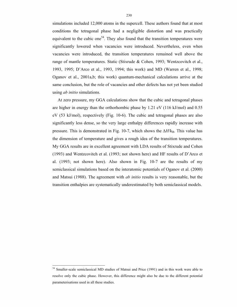
230
simulations included 12,000 atoms in the supercell. These authors found that at most
conditions the tetragonal phase had a negligible distortion and was practically
equivalent to the cubic one54. They also found that the transition temperatures were
significantly lowered when vacancies were introduced. Nevertheless, even when
vacancies were introduced, the transition temperatures remained well above the
range of mantle temperatures. Static (Stixrude & Cohen, 1993; Wentzcovitch et al.,
1993, 1995; D’Arco et al., 1993, 1994; this work) and MD (Warren et al., 1998;
Oganov et al., 2001a,b; this work) quantum-mechanical calculations arrive at the
same conclusion, but the role of vacancies and other defects has not yet been studied
using ab initio simulations.
At zero pressure, my GGA calculations show that the cubic and tetragonal phases
are higher in energy than the orthorhombic phase by 1.21 eV (116 kJ/mol) and 0.55
eV (53 kJ/mol), respectively (Fig. 10-6). The cubic and tetragonal phases are also
significantly less dense, so the very large enthalpy differences rapidly increase with
pressure. This is demonstrated in Fig. 10-7, which shows the ∆H/kB. This value has
the dimension of temperature and gives a rough idea of the transition temperatures.
My GGA results are in excellent agreement with LDA results of Stixrude and Cohen
(1993) and Wentzcovitch et al. (1993; not shown here) and HF results of D’Arco et
al. (1993; not shown here). Also shown in Fig. 10-7 are the results of my
semiclassical simulations based on the interatomic potentials of Oganov et al. (2000)
and Matsui (1988). The agreement with ab initio results is very reasonable, but the
transition enthalpies are systematically underestimated by both semiclassical models.
54 Smaller-scale semiclassical MD studies of Matsui and Price (1991) and in this work were able to
resolve only the cubic phase. However, this difference might also be due to the different potential
parameterisations used in all these studies.

231
Fig. 10-6. E(V) curves for the orthorhombic, tetragonal, and cubic phases of MgSiO3 perovskite: GGA calculations. Minimum energy of the Pbnm phase is set as the reference zero. Energies are per formula unit.
Stixrude and Cohen (1993) have shown that both cubic and tetragonal phases actually
correspond to local energy maxima. This has since been confirmed in many studies (e.g.,
Parlinsky & Kawazoe, 2000; Warren et al., 1998), which found that both tetragonal and
cubic phases are dynamically unstable. The instability is due to the relatively small size
of the Mg2+ cation, which cannot support the large cage of the ideal cubic structure –
and the cage accordingly collapses.
If the transition is purely displacive, the high-symmetry cubic and tetragonal
structures will be the transition states; the real structure will be dynamically disordered,
hopping both ways through these barriers (see a scheme shown in Fig. 4-1). The barrier
height (i.e., ∆H) will be directly related to the transition temperature, which is the
temperature of the onset of the dynamical disorder. ∆H/kB will then be a correct
semiquantitative estimate of the transition temperature, and this estimate significantly
exceeds the mantle temperatures.

232
Fig. 10-7. Enthalpy differences (∆H/kB, in units of temperature) cubic-orthorhombic and tetragonal-orthorhombic as a function of pressure. Results based on the LDA (Stixrude & Cohen, 1993) and GGA (this work) are shown along with the results based on semiclassical interatomic potentials of Oganov et al. (2000) [lines] and Matsui (1988) [solid circles].
In the other limit, the transition may be of the pure order-disorder type. In this case,
the structure is also locally distorted, but all disorder is static. In this limit, there is no
hopping over the barrier, because it is too high compared to kBTc, i.e. the transition
temperature is much lower than ∆H/kB. Computer simulations suggest that the
Pbnm→Pm−3m transition in Mg-pv is intermediate between the pure order-disorder and
displacive types. Apart from the energy of rigid rotations of the SiO6 octahedra, there
will be an important contribution from the bending of the O-Si-O angles within these
octahedra. The latter contribution arises as a consequence of any static positional
disorder of the O atoms. Keeping in mind that the first energy term is underestimated by
the model pair potentials, at least by those of Matsui (1988) and Oganov et al. (2000)
and the angle-bending terms are not present in these models at all, one expects that
semiclassical simulations will give a lower bound to the transition temperatures.
However, my semiclassical MD simulations (Fig. 10-8), as well as those of Matsui and
Price (1991) and Chaplot et al. (1998) give temperatures that are way too high for the
lower mantle.
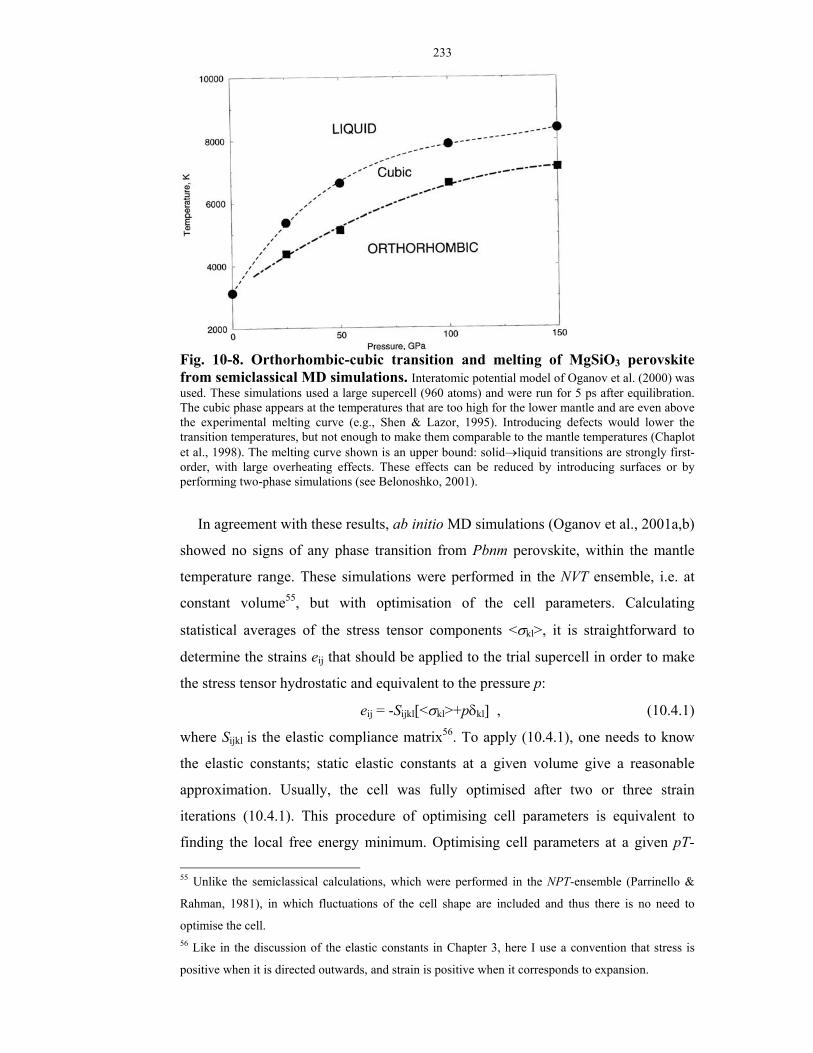
233
Fig. 10-8. Orthorhombic-cubic transition and melting of MgSiO3 perovskite from semiclassical MD simulations. Interatomic potential model of Oganov et al. (2000) was used. These simulations used a large supercell (960 atoms) and were run for 5 ps after equilibration. The cubic phase appears at the temperatures that are too high for the lower mantle and are even above the experimental melting curve (e.g., Shen & Lazor, 1995). Introducing defects would lower the transition temperatures, but not enough to make them comparable to the mantle temperatures (Chaplot et al., 1998). The melting curve shown is an upper bound: solid→liquid transitions are strongly first-order, with large overheating effects. These effects can be reduced by introducing surfaces or by performing two-phase simulations (see Belonoshko, 2001).
In agreement with these results, ab initio MD simulations (Oganov et al., 2001a,b)
showed no signs of any phase transition from Pbnm perovskite, within the mantle
temperature range. These simulations were performed in the NVT ensemble, i.e. at
constant volume55, but with optimisation of the cell parameters. Calculating
statistical averages of the stress tensor components <σkl>, it is straightforward to
determine the strains eij that should be applied to the trial supercell in order to make
the stress tensor hydrostatic and equivalent to the pressure p:
eij = -Sijkl[<σkl>+pδkl] , (10.4.1)
where Sijkl is the elastic compliance matrix56. To apply (10.4.1), one needs to know
the elastic constants; static elastic constants at a given volume give a reasonable
approximation. Usually, the cell was fully optimised after two or three strain
iterations (10.4.1). This procedure of optimising cell parameters is equivalent to
finding the local free energy minimum. Optimising cell parameters at a given pT- 55 Unlike the semiclassical calculations, which were performed in the NPT-ensemble (Parrinello &
Rahman, 1981), in which fluctuations of the cell shape are included and thus there is no need to
optimise the cell. 56 Like in the discussion of the elastic constants in Chapter 3, here I use a convention that stress is
positive when it is directed outwards, and strain is positive when it corresponds to expansion.

234
point, one can see whether the phase remains orthorhombic or has transformed, e.g.
to the cubic phase (see Fig. 10-9)57. For the optimised cell, one can also determine
the elastic constants at given p and T from stress-strain relations (Oganov et al.,
2001b). Five pT-points have been studied: (38 GPa, 1500 K), (38 GPa, 2500 K), (38
GPa, 3500 K), (88 GPa, 1500 K), and (136 GPa, 4500 K). Although the simulations
do show the orthorhombic distortion decrease with temperature, even at the highest
temperatures probed the structure remained orthorhombic. One point (38 GPa, 3500
K) is very close to melting and had very vigorous large-amplitude thermal motion of
atoms. It is remarkable that even at these conditions Mg-pv remained orthorhombic.
To summarise, our results and the general majority of evidence indicate stability
of the orthorhombic (Pbnm) Mg-pv throughout the lower mantle. Interestingly,
another group (Stixrude, 2001) recently performed ab initio MD simulations, very
similar to mine and in the same p-T range. However, that group arrived at an
opposite conclusion. Their simulations found the Pmmn phase, seemingly supporting
the experimental findings of Shim et al. (2001). Most probably, the difference is due
to less accurate pseudopotentials used by that group. This point needs further
research.
a b Fig. 10-9. Stress tensor and crystal structure of MgSiO3 perovskite at 88 GPa and 3500 K from ab initio MD simulations. (a) In the optimised cell, the stress tensor is hydrostatic. In this figure, an example from a simulation at 88 GPa and 3500 K is shown. (b) A snapshot of the structure of MgSiO3 perovskite at 88 GPa and 3500 K in the optimised cell. Such simulations show that the orthorhombic structure is stable throughout the lower mantle pressure-temperature regime. 10.5. Equation of state and mantle geotherm.
57 In this way, one could have a metastable low-symmetry phase persisting in the stability domain of
the high-symmetry phase. Such problems do not occur in Mg-pv, where the expected transitions are
tricritical or even second-order.
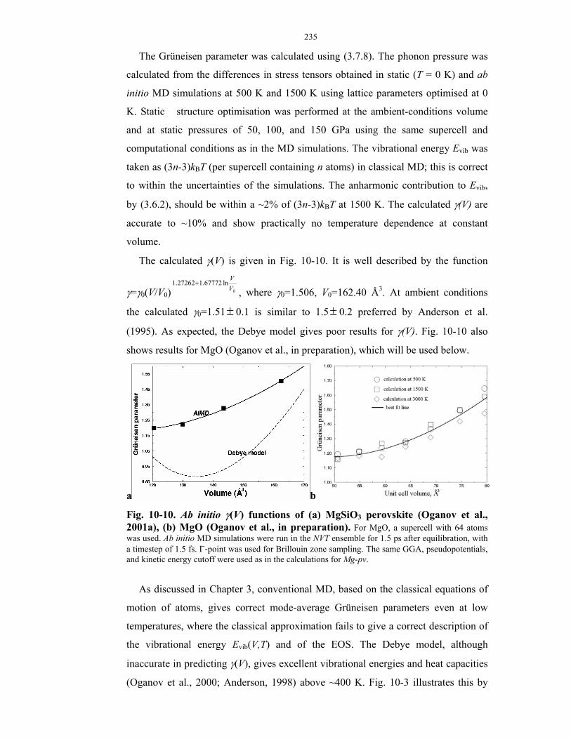
235
The Grüneisen parameter was calculated using (3.7.8). The phonon pressure was
calculated from the differences in stress tensors obtained in static (T = 0 K) and ab
initio MD simulations at 500 K and 1500 K using lattice parameters optimised at 0
K. Static structure optimisation was performed at the ambient-conditions volume
and at static pressures of 50, 100, and 150 GPa using the same supercell and
computational conditions as in the MD simulations. The vibrational energy Evib was
taken as (3n-3)kBT (per supercell containing n atoms) in classical MD; this is correct
to within the uncertainties of the simulations. The anharmonic contribution to Evib,
by (3.6.2), should be within a ~2% of (3n-3)kBT at 1500 K. The calculated γ(V) are
accurate to ~10% and show practically no temperature dependence at constant
volume.
The calculated γ(V) is given in Fig. 10-10. It is well described by the function
γ=γ0(V/V0) 0
ln67772.127262.1VV
+, where γ0=1.506, V0=162.40 Å3. At ambient conditions
the calculated γ0=1.51 ± 0.1 is similar to 1.5 ± 0.2 preferred by Anderson et al.
(1995). As expected, the Debye model gives poor results for γ(V). Fig. 10-10 also
shows results for MgO (Oganov et al., in preparation), which will be used below.
a b
Fig. 10-10. Ab initio γ(V) functions of (a) MgSiO3 perovskite (Oganov et al., 2001a), (b) MgO (Oganov et al., in preparation). For MgO, a supercell with 64 atoms was used. Ab initio MD simulations were run in the NVT ensemble for 1.5 ps after equilibration, with a timestep of 1.5 fs. Γ-point was used for Brillouin zone sampling. The same GGA, pseudopotentials, and kinetic energy cutoff were used as in the calculations for Mg-pv.
As discussed in Chapter 3, conventional MD, based on the classical equations of
motion of atoms, gives correct mode-average Grüneisen parameters even at low
temperatures, where the classical approximation fails to give a correct description of
the vibrational energy Evib(V,T) and of the EOS. The Debye model, although
inaccurate in predicting γ(V), gives excellent vibrational energies and heat capacities
(Oganov et al., 2000; Anderson, 1998) above ~400 K. Fig. 10-3 illustrates this by
236
comparing CV obtained by Debye model and full harmonic calculations, both of
which were based on the same model of interatomic interactions (Oganov et al.,
2000). Therefore, I used Debye model (based on the calculated ab initio static elastic
constants – Table 10-4 and Fig. 10-11) to determine the first approximation to
Evib(V,T).
a b
Fig. 10-11. Athermal elastic constants of MgSiO3 perovskite as a function of pressure. (a) GGA data of Oganov et al. (2001a) with shifted pressure scale, (b) LDA results of Karki et al. (1997). GGA calculations give ∂G/∂p=1.88 at 0 GPa, close to the experimental value of 1.8 (Sinelnikov et al., 1998).
Table 10-4. Elastic properties of MgSiO3 perovskite as a function of pressure (at 298 K)a
Pressure (GPa) 0 30 60 90 120 150
V0 , Å3 162.4 148.0 138.1 130.6 124.5 119.5 C11, GPa 492 629 746 851 947 1036 C22 550 727 888 1044 1196 1344
C33 472 661 833 995 1150 1298 C12 142 246 349 449 546 639
C13 148 216 287 360 433 505 C23 160 237 311 385 457 528 C44 213 264 309 351 394 433 C55 187 221 247 272 296 319 C66 154 206 249 293 338 384 K , GPa 267 379 483 583 681 775 G 180 225 261 294 325 355
a - Cij values in this table were obtained by 3rd order polynomials interpolations of Cij from Fig. 10-11a.
Isothermal Mie-Grüneisen EOSs, fitted by the Vinet function, are given for
several temperatures in Table 10-5. Table 10-6 gives a summary of thermoelastic

237
parameters of MgSiO3 perovskite. Comparing these tables, one can see that zero-
point contribution dominates the phonon pressure at ambient conditions.
Table 10-5. Ab initio thermal EOS of MgSiO3 perovskite.
T, K static 0 1500 2000 2500 3000 4000
V0, Å3 160.2 162.1 167.9 170.9 174.2 177.9 187.2
K0, GPa 279.7 269.9 228.3 210.6 192.3 173.5 134.4 K’ 4.02 4.07 4.36 4.49 4.63 4.78 5.13
Table 10-6. Thermoelastic parameters of MgSiO3 perovskite from theory and experiment. Source V0, Å3 K0, GPa K’ (∂KT/∂T)p,
10-3GPa/K TpK∂∂
∂ T2
,
10-5 K-1
γ0 q0 α0, 10-5 K-1
Ab initio simulations LDAa 160.74 266 4.2 - - - - - LDAb 157.50 259 3.9 - - - - - LDAc 162.47 257 4.02 - - - - - LDAd 164.1 247 3.97 -31 32 1.63 2.0e 2.15 GGA (162.4) 267 4.10 -21 15 1.51 1.27e 1.86
Experiment 1f 162.3 259.5 3.69 -17 - (1.4) 1.4 1.8-2.2 2f (162.3) (261) (4) -28 - 1.42 2.0 1.7 3f,g (162.2) (261) (4) -22 8 1.25 1 1.65
Exp. range
162.4±1 247-272 3.6-7 -17 to -63 - 1.3-2.2 ~1-2.5 1.4-3.3
a – LAPW results of Stixrude & Cohen (1993). b – Pseudopotential calculations of Wentzcovitch et al. (1995). c – Pseudopotential calculations of Karki (personal communication, 1997). d – Quasiharmonic simulations of Karki et al. (2001), based on the LDA and pseudopotential plane
wave method. e – Values given in this table correspond to the ambient conditions. Both my simulations (Oganov et
al., 2001a) and those of Karki et al. (2001) found that q varies very strongly with volume. f – 1: Fiquet et al. (2000), 2: Shim & Duffy (2000), 3: Gillet et al. (2000). g – Work of Gillet et al. (2000), based on Raman spectroscopic measurements combined with
experimental room-temperature EOS, resulted in several distinct models. Numbers given here correspond to their preferred model.
Thermal expansion was calculated as α=γCV/KTV. Thus calculated α is consistent
(to within a few percent) with those determined directly from the ab initio MD
optimised cell volumes at 38 GPa and 88 GPa in the temperature interval 1500-3500
K. Fig. 10-12 gives a comparison of the theoretical (Oganov et al., 2001; Karki et al.,
2001) thermal expansion coefficients as a function of pressure and temperature.
Several experimental results at 1 atm are also shown. Theoretical calculations are in
good agreement with each other, being practically indistinguishable above 50 GPa.
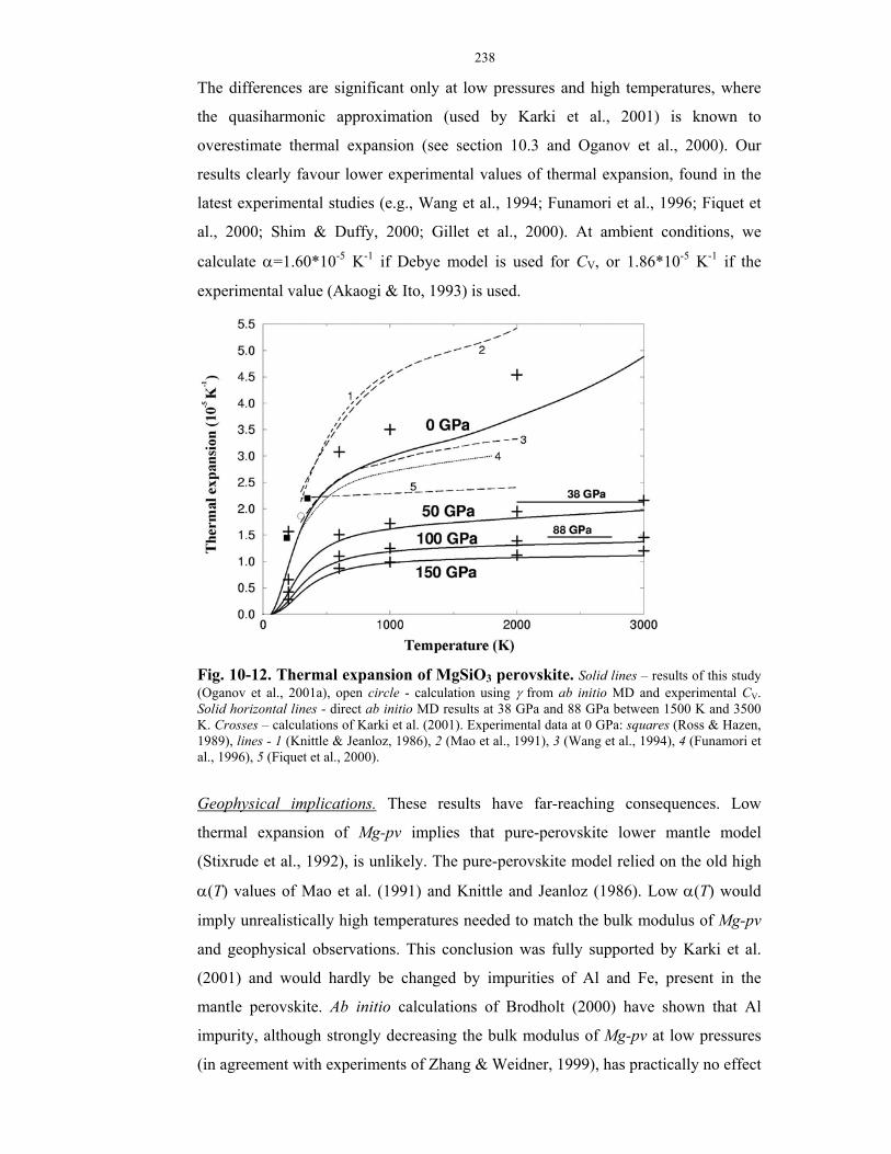
238
The differences are significant only at low pressures and high temperatures, where
the quasiharmonic approximation (used by Karki et al., 2001) is known to
overestimate thermal expansion (see section 10.3 and Oganov et al., 2000). Our
results clearly favour lower experimental values of thermal expansion, found in the
latest experimental studies (e.g., Wang et al., 1994; Funamori et al., 1996; Fiquet et
al., 2000; Shim & Duffy, 2000; Gillet et al., 2000). At ambient conditions, we
calculate α=1.60*10-5 K-1 if Debye model is used for CV, or 1.86*10-5 K-1 if the
experimental value (Akaogi & Ito, 1993) is used.
Fig. 10-12. Thermal expansion of MgSiO3 perovskite. Solid lines – results of this study (Oganov et al., 2001a), open circle - calculation using γ from ab initio MD and experimental CV. Solid horizontal lines - direct ab initio MD results at 38 GPa and 88 GPa between 1500 K and 3500 K. Crosses – calculations of Karki et al. (2001). Experimental data at 0 GPa: squares (Ross & Hazen, 1989), lines - 1 (Knittle & Jeanloz, 1986), 2 (Mao et al., 1991), 3 (Wang et al., 1994), 4 (Funamori et al., 1996), 5 (Fiquet et al., 2000).
Geophysical implications. These results have far-reaching consequences. Low
thermal expansion of Mg-pv implies that pure-perovskite lower mantle model
(Stixrude et al., 1992), is unlikely. The pure-perovskite model relied on the old high
α(T) values of Mao et al. (1991) and Knittle and Jeanloz (1986). Low α(T) would
imply unrealistically high temperatures needed to match the bulk modulus of Mg-pv
and geophysical observations. This conclusion was fully supported by Karki et al.
(2001) and would hardly be changed by impurities of Al and Fe, present in the
mantle perovskite. Ab initio calculations of Brodholt (2000) have shown that Al
impurity, although strongly decreasing the bulk modulus of Mg-pv at low pressures
(in agreement with experiments of Zhang & Weidner, 1999), has practically no effect

239
above 30 GPa. With accurate thermoelastic parameters and EOS of Mg-pv, now it
should be straightforward to determine the most likely composition of the lower
mantle; this result would be very important for understanding the dynamics of the
mantle and global chemistry of the Earth.
With the data presented here we can construct a thermal profile of the lower
mantle. For the convecting lower mantle, the average temperature as a function of
depth (geotherm) should increase at least adiabatically. As discussed by Jackson
(1998), PREM (Dziewonski & Anderson, 1981) indicates adiabatic lower mantle,
while another major global Earth’s seismological model – ak135 (Kennett et al.,
1995) – is consistent with large superadiabaticity in this region.
Here I construct a new adiabatic geotherm (Oganov et al., in preparation), which
will serve us as a useful reference. This adiabatic geotherm is constructed on the
basis of the γ(V) functions (Fig. 10-10) of Mg-pv and periclase (MgO), which
together account for ~90-95 vol. % of the lower mantle. The adiabatic temperature
profile is expressed as the following integral:
T(z) = T(670 km) + zz
VTz
kmz
ddlnd)(
6701
∫=
ργ , (10.5.1)
where I use T(670 km)=1873±100 K determined from phase equilibria (Ito &
Katsura, 1989) and geophysical (PREM) density profile ρ(z)58. Fig. 10-13 shows that
two adiabats obtained with γ(V) of MgSiO3 and MgO (thick dashed lines) are
practically indistinguishable; therefore, we have an accurately constrained adiabatic
geotherm (between these two adiabats). This adiabatic geotherm is quite similar to
the classical geotherms of Brown and Shankland (1981) and Anderson (1982), both
of which included a small superadiabatic gradient.
Later in this chapter I consider lateral temperature variations in the lower mantle.
These are extremely important for the understanding of the Earth’s dynamics, but
have been poorly understood to date. The breakthrough was achieved (Oganov et al.,
2001b) by combining the state of the art of seismic tomography and hitherto
unprecedented ab initio MD calculations of the elastic constants at mantle
temperatures and pressures.
58 PREM density profile is used instead of using theoretical equations of state of minerals. It is
preferable to use as many accurate seismological data as possible to construct a good geotherm. Using
mineral equations of state, on the other hand, would be useful in discriminating between different
compositional models of the mantle.

240
Fig. 10-13. Adiabatic geotherm (this work) in comparison with the geotherms of Brown and Shankland (1981) and Anderson (1982).
10.6. Elastic constants at mantle temperatures and pressures.
The athermal elastic constants as a function of pressure (Oganov et al., 2001a) are
shown in Fig. 10-11. My results are very similar to those of Karki et al. (1997). At 1
atm, the agreement with experimental results (Yeganeh-Haeri, 1994) is remarkably
good.
We were also able to perform ab initio MD calculations of the elastic constants of
MgSiO3 perovskite at lower mantle conditions – including temperature. We believe
that these are the first ab initio MD calculations of the elastic constants of any
material at non-zero temperatures. Such calculations are extremely computationally
demanding. The elastic constants were calculated for the optimised supercells, from
non-linear stress-strain relations with +2% and –2% strains (see Fig. 10-14).
In seismology, the relevant elastic constants are the adiabatic ones; in the NVT-
ensemble one calculates the isothermal constants. It is easy to transform the
isothermal values into adiabatic (and vice versa) using (3.10.15). The temperature
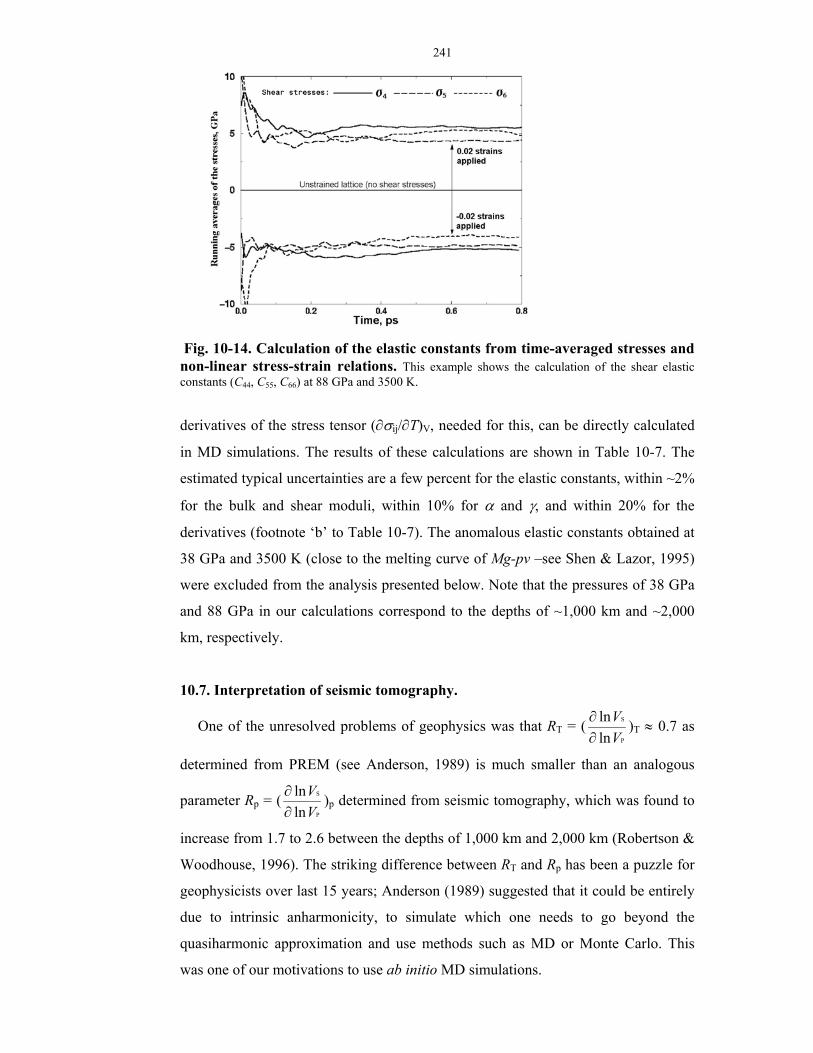
241
Fig. 10-14. Calculation of the elastic constants from time-averaged stresses and non-linear stress-strain relations. This example shows the calculation of the shear elastic constants (C44, C55, C66) at 88 GPa and 3500 K.
derivatives of the stress tensor (∂σij/∂T)V, needed for this, can be directly calculated
in MD simulations. The results of these calculations are shown in Table 10-7. The
estimated typical uncertainties are a few percent for the elastic constants, within ~2%
for the bulk and shear moduli, within 10% for α and γ, and within 20% for the
derivatives (footnote ‘b’ to Table 10-7). The anomalous elastic constants obtained at
38 GPa and 3500 K (close to the melting curve of Mg-pv –see Shen & Lazor, 1995)
were excluded from the analysis presented below. Note that the pressures of 38 GPa
and 88 GPa in our calculations correspond to the depths of ~1,000 km and ~2,000
km, respectively.
10.7. Interpretation of seismic tomography.
One of the unresolved problems of geophysics was that RT = (P
S
lnln
VV
∂∂ )T ≈ 0.7 as
determined from PREM (see Anderson, 1989) is much smaller than an analogous
parameter Rp = (P
S
lnln
VV
∂∂ )p determined from seismic tomography, which was found to
increase from 1.7 to 2.6 between the depths of 1,000 km and 2,000 km (Robertson &
Woodhouse, 1996). The striking difference between RT and Rp has been a puzzle for
geophysicists over last 15 years; Anderson (1989) suggested that it could be entirely
due to intrinsic anharmonicity, to simulate which one needs to go beyond the
quasiharmonic approximation and use methods such as MD or Monte Carlo. This
was one of our motivations to use ab initio MD simulations.
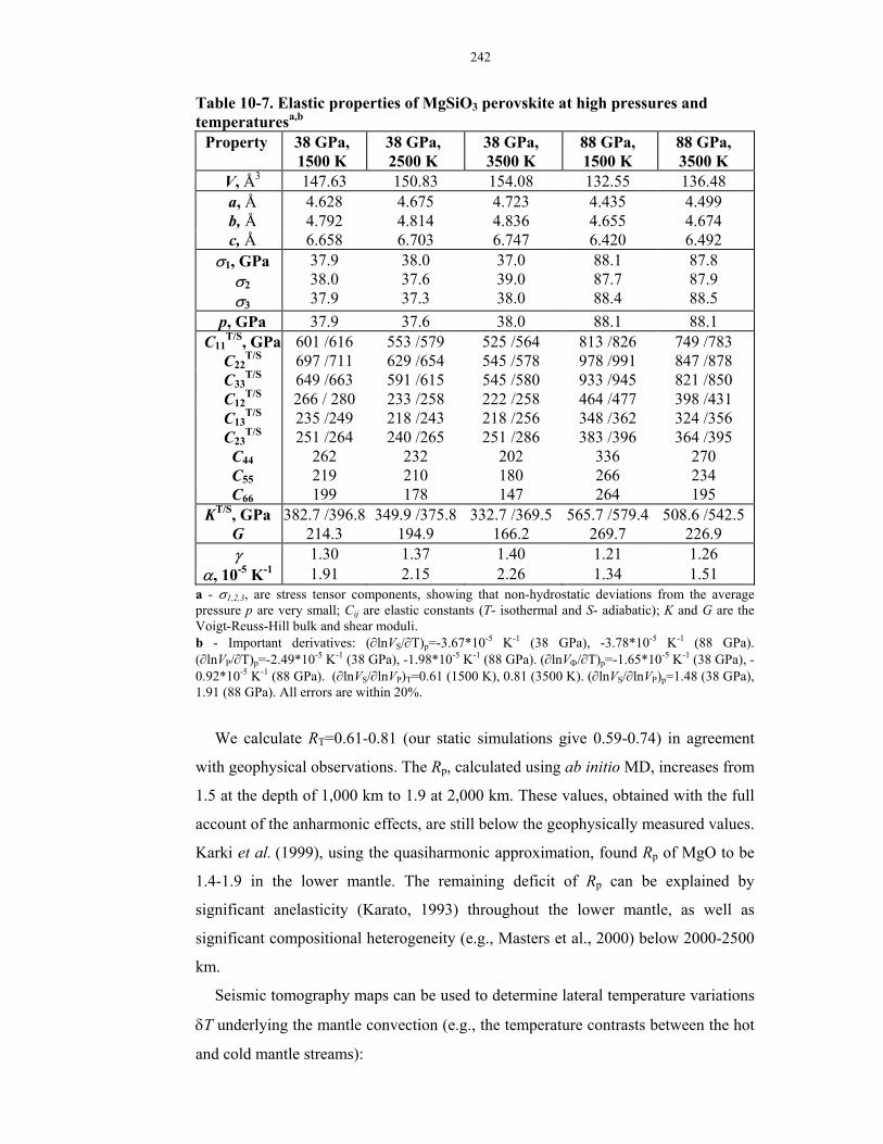
242
Table 10-7. Elastic properties of MgSiO3 perovskite at high pressures and temperaturesa,b
Property 38 GPa, 1500 K
38 GPa, 2500 K
38 GPa, 3500 K
88 GPa, 1500 K
88 GPa, 3500 K
V, Å3 147.63 150.83 154.08 132.55 136.48 a, Å 4.628 4.675 4.723 4.435 4.499 b, Å 4.792 4.814 4.836 4.655 4.674 c, Å 6.658 6.703 6.747 6.420 6.492
σ1, GPa σ2 σ3
37.9 38.0 37.9
38.0 37.6 37.3
37.0 39.0 38.0
88.1 87.7 88.4
87.8 87.9 88.5
p, GPa 37.9 37.6 38.0 88.1 88.1 C11
T/S, GPa 601 /616 553 /579 525 /564 813 /826 749 /783 C22
T/S 697 /711 629 /654 545 /578 978 /991 847 /878 C33
T/S 649 /663 591 /615 545 /580 933 /945 821 /850 C12
T/S 266 / 280 233 /258 222 /258 464 /477 398 /431 C13
T/S 235 /249 218 /243 218 /256 348 /362 324 /356 C23
T/S 251 /264 240 /265 251 /286 383 /396 364 /395 C44 262 232 202 336 270 C55 219 210 180 266 234 C66 199 178 147 264 195
KT/S, GPa 382.7 /396.8 349.9 /375.8 332.7 /369.5 565.7 /579.4 508.6 /542.5 G 214.3 194.9 166.2 269.7 226.9 γ 1.30 1.37 1.40 1.21 1.26
α, 10-5 K-1 1.91 2.15 2.26 1.34 1.51 a - σ1,2,3, are stress tensor components, showing that non-hydrostatic deviations from the average pressure p are very small; Cij are elastic constants (T- isothermal and S- adiabatic); K and G are the Voigt-Reuss-Hill bulk and shear moduli. b - Important derivatives: (∂lnVS/∂T)p=-3.67*10-5 K-1 (38 GPa), -3.78*10-5 K-1 (88 GPa). (∂lnVP/∂T)p=-2.49*10-5 K-1 (38 GPa), -1.98*10-5 K-1 (88 GPa). (∂lnVΦ/∂T)p=-1.65*10-5 K-1 (38 GPa), -0.92*10-5 K-1 (88 GPa). (∂lnVS/∂lnVP)T=0.61 (1500 K), 0.81 (3500 K). (∂lnVS/∂lnVP)p=1.48 (38 GPa), 1.91 (88 GPa). All errors are within 20%.
We calculate RT=0.61-0.81 (our static simulations give 0.59-0.74) in agreement
with geophysical observations. The Rp, calculated using ab initio MD, increases from
1.5 at the depth of 1,000 km to 1.9 at 2,000 km. These values, obtained with the full
account of the anharmonic effects, are still below the geophysically measured values.
Karki et al. (1999), using the quasiharmonic approximation, found Rp of MgO to be
1.4-1.9 in the lower mantle. The remaining deficit of Rp can be explained by
significant anelasticity (Karato, 1993) throughout the lower mantle, as well as
significant compositional heterogeneity (e.g., Masters et al., 2000) below 2000-2500
km.
Seismic tomography maps can be used to determine lateral temperature variations
δT underlying the mantle convection (e.g., the temperature contrasts between the hot
and cold mantle streams):
243
δT = VVδ /(∂lnV/∂T)p ; (10.7.1)
(∂lnV/∂T)p are given in Table 10-7 for different seismic velocities. To avoid the
poorly known attenuation effects and minimise even poorer known compositional
effects, it is better to use bulk sound velocity (VΦ) maps.
Using seismic tomography maps of Masters et al. (2000) (with maximum velocity
contrast φ
φ
VV∆
= 1.4% at 1225 km and 2195 km), one gets (Oganov et al., 2001b) the
maximum temperature contrast between the hot and cold streams increasing from
900 K to 1500 K between 1000 and 2000 km. Linear extrapolation gives ~700 K at
the top and 2100 K at the bottom of the lower mantle. The root-mean square
temperature variations are ~150-250 K across the lower mantle. These contrasts
turned out to be large; much smaller than those of Yuen et al. (1993), but larger than
those of Forte and Mitrovica (2001) or Castle et al. (2000). These values will play an
important role in the future models of the Earth’s mantle and its dynamics and can be
used as important constraints in numerical models of the mantle convection.
If we use shear velocity maps, much smaller temperature contrasts are obtained
for the 2,000 km depth and below. From the VS maps of Masters et al. (2000)
(maximum S
S
VV∆ = 3.6% at 1225 km and 2195 km) we get ~1000 K throughout.
Systematically lower temperature contrasts result from shear velocity maps at 2000
km depth and below. This systematic difference could be due to the hot masses,
rising from the core-mantle boundary, being depleted in Fe due to a reaction (Knittle
& Jeanloz, 1991) between the core and mantle, driving Fe from the silicate mantle
into the metallic core. This hypothesis, supported by an independent study of Forte
and Mitrovica (2001), implies that the core is still growing (although, most probably,
very slowly). Minor differences in the Fe content have only a reduced effect on the
bulk velocity, but are important for the shear velocities: hot Fe-depleted and cold Fe-
enriched materials can have the same shear wave velocities. Lateral variations in the
Fe content can explain the anticorrelation between the shear and bulk velocities
observed (e.g., Masters et al., 2000) near the core-mantle boundary. However, this
does not explain why the anomalies on the bulk velocity maps undergo a reversal
near the core-mantle boundary (i.e. low-velocity zones at the core-mantle boundary
underlay high-velocity zones of the rest of the lower mantle): such a reversal would

244
be more expected for the shear velocities (for which it does not happen). This puzzle
still remains to be solved; whatever is the answer, it is important that the temperature
contrasts obtained from the bulk velocities must be the most reliable, at least outside
the anomalous core-mantle boundary region.
Our temperature contrasts are ~2-4 times smaller than estimates of Yuen et al.
(1993), which were obtained using extremely uncertain extrapolations of temperature
derivatives of shear wave velocities and would suggest partial melting of the lower
mantle. Present results can support partial melting only near the core-mantle
boundary. This is clarified in Fig. 10-15.
For the core side of the core-mantle boundary experiments of Boehler (1996)
suggest T~4000 K. In good agreement with this, ab initio simulations (D. Alfé,
personal communication) give 4100-4400 K. This gives the highest temperature in
the mantle. From this and from our temperature contrasts we see that the minimum
temperature of the mantle near the core-mantle boundary is 2000-2200. Using the
starting temperature T(670 km) = 1873 K, core-mantle boundary temperature (4000-
4400 K), our mantle adiabat and temperature contrasts, one can obtain a very
interesting general picture (Fig. 10-15). Comparing this picture with experimental
solidus of pyrolite determined by Zerr et al. (1998), we expect some degree of partial
melting, restricted only to the lowermost ~300 km of the lower mantle. This would
have important implications for the anomalous properties of the core-mantle D’’
layer. The melt present in the D’’ should give rise to high electrical conductivity of
this layer, due to the diffusion of all ionic species in the melt. Fig. 10-15 suggests
that the cold streams seem to be adiabatic throughout the lower mantle, while the hot
streams are strongly superadiabatic. Below 2000 km we observe a strong asymmetry
of temperatures relative to the adiabatic geotherm. The simplest way to explain this
is to postulate that the average mantle temperatures are superadiabatic below 2000
km, due to the influence of the thermal boundary at 2890 km. Seismic tomography
maps (Masters et al., 2000) give hot and cold anomalies as roughly equal, giving
some support to this idea (in this case the superadiabatic geotherm would be ~500 K
above the adiabat near the core-mantle boundary).

245
Fig. 10-15. Schematic temperature distribution in the lower mantle. Two-headed arrows indicate the maximum temperature contrasts (the lower arrow gives the lowest possible temperature at a given depth; the upper arrow gives the maximum temperature). Thick dashed curve – lower mantle adiabatic geotherm from Fig. 10-13 (depicted as two almost coinciding adiabats).
Kesson et al. (1998) estimated that lithospheric slabs should be at least ~650 K
colder than surrounding mantle if they are to sink to the core-mantle boundary and at
least 250 K colder to reach the depth of 1,100 km. Our maximum cold temperature
anomalies suggest that most slabs should be able to reach the core-mantle boundary,
but some might stop at an intermediate depth. Neutrally buoyant slabs will be
dissolved by the convecting mantle; some tomographic maps show most slabs
disappearing in the middle of the lower mantle (Kennett et al., 1998), while others
(Masters et al., 2000) show that most slabs do reach the core-mantle boundary.
The next important step is to estimate the extent of chemical heterogeneity and
anelasticity in the lower mantle and construct a 3D- mineralogical model of the
Earth’s mantle. With improved seismic tomography models and mineral physics data
this problem can be solved in foreseeable future. I believe that computational mineral
physics will play an important role in solving this and many other geologically
important and exciting problems.

246
Chapter 11. Conclusions. In this thesis I have presented some of the fundamentals of modern computer
simulations of materials and a number of their applications to minerals. A few new
equations have been derived and a new classification of phase transitions developed.
Simulation methods used in this study ranged from semiclassical to quantum-
mechanical and from static to lattice-dynamical and molecular dynamics. With these
methods, it was possible to solve a few long-standing problems that could not be
resolved experimentally. A series of unusual metastable phase transitions have been
predicted for the Al2SiO5 polymorphs. These simulations clarified the nature of
fivefold-coordinated states of Si in high-density silicates. Such issues have been
addressed as high-pressure stability of the Al2SiO5 polymorphs, nature of anomalous
antiordering in albite (NaAlSi3O8), equation of state of MgSiO3 perovskite, its
thermal expansion, stability and elasticity at high temperatures and pressures of the
Earth’s mantle, and the temperature distribution in the mantle. As clear from this list
and from the list of the methods, such studies span a unique range of scales – from
the subatomic scale (in quantum-mechanical simulations) and the scale of atoms and
their interactions, to the scale of macroscopic crystals and their properties and,
finally, to the scale of large parts of the Earth and planetary chemistry and dynamics.
The results presented in this thesis have significantly extended our understanding
of the Earth and especially its mantle. However, a large number of problems still
remain open, and here I mention a few. E.g., there is no commonly accepted
compositional model of the lower mantle. There is no common explanation for the
mid-mantle discontinuities, e.g. those at 900 km and 1200 km. Practically nothing
certain is known about the core-mantle boundary region and the processes of
equilibration between the core and mantle that are going on there. It is of particular
importance to know whether or not large amounts of Si and K are stored in the
Earth’s core. The effects of Fe on mantle minerals and the spin state of Fe in these
minerals are also among the important problems, but present-day computational
methods cannot give a reliable description of the electronic structure of transition
metal oxides and silicates. New computational methods are needed for such
complicated problems.
247
References Adams D.M., Hatton P.D., Heath A.E., Russell D.R. (1988). X-ray diffraction
measurements on potassium nitrate under high pressure using synchrotron
radiation. J. Phys. C21, 505-515.
Agoshkov V.M. (1985). Calculation of thermodynamic properties of minerals based
on a model of the vibrational spectrum for silicates and oxides. Geokhimiya, No.
10, 1441-1454. (in Russian).
Agoshkov V.M., Kieffer S.W., McMillan P.F. (1994). Lattice dynamics and
thermodynamic properties of minerals. In: Advanced mineralogy, v. 1, 419-430.
Marfunin A.S. (editor), Springer-Verlag: Berlin.
Ahmed-Zaid I. & Madon M. (1991). A high-pressure form of Al2SiO5 as a possible
host of aluminium in the lower mantle. Nature 353, 426-428.
Ahmed-Zaid I. & Madon M. (1995). Electron microscopy of high-pressure phases
synthesized from natural garnets in a diamond anvil cell : Implications for the
mineralogy of the lower mantle. Earth Planet. Sci. Lett. 129, 233-247.
Akaogi M. & Ito E. (1993). Heat capacity of MgSiO3 perovskite. Geophys. Res. Lett.
20, 105-108.
Akaogi M., Yusa H., Shiraishi K. & Suzuki T. (1995). Thermodynamic properties of
alpha-quartz, coesite, and stishovite and equilibrium phase-relations at high
pressures and high temperatures. J. Geophys. Res. 100, 22337-22347.
Alan D.R. & Nelmes R.J. (1996). The structural pressure dependence of potassium
titanyl phosphate (KTP). to 8 GPa. J. Phys.: Condens. Matter 8, 2337-2363.
Alavi A., Lozovoi A., & Finnis M.W. (1999). Pressure-induced isostructural phase
transition in Al-rich NiAl alloys. Phys Rev. Lett. 83, 979-982.
Alberti, A., Sacerdoti, M., Quartieri, S., & Vezzalini, G. (1999). Heating-induced
phase transformation in zeolite brewsterite: new 4- and 5-coordinated (Si,Al) sites.
Phys. Chem. Minerals 26, 181-186.
Alexandrov K.S. & Prodaivoda G.T. (1993). Elastic properties of minerals.
Crystallografiya 38, 214-234. (in Russian).
Alfé D., Gillan M.J., & Price G.D. (1999). The melting curve of iron at the pressures
of the Earth’s core from ab initio calculations. Nature 401, 462-464.
Alfé D., Gillan M.J., & Price G.D. (2000). Constraints on the composition of the
Earth's core from ab initio calculations. Nature 405, 172-175.
248
Allègre C.J., Manhes G., & Göpel C. (1995a). The age of the Earth. Geochim.
Cosmochim. Acta 59, 1445-1456.
Allègre C.J., Poirier J.-P., Humler E., & Hofmann A.W. (1995b). The chemical
composition of the Earth. Earth Planet. Sci. Lett. 134, 515-526.
Allen L.C. (1989). Electronegativity is the average one-electron energy of the valence-
shell electrons in ground-state free atoms. J. Am. Chem. Soc. 111, 9003-9014.
Allen M.P. & Tildesley D.J. (1987). Computer Simulation of Liquids. Clarendon
Press: Oxford, 385 pp.
Ancilotto F., Chiarotti G.L., Scandolo S., & Tosatti E. (1997). Dissociation of methane
into hydrocarbons at extreme (planetary) pressure and temperature. Science 275,
1288-1290.
Anders E. & Ebihara M. (1982). Solar system abundances of the elements. Geochim.
Cosmochim. Acta 46, 2363-2380.
Anderson D.L. (1989). Theory of the Earth. Blackwell Scientific Publications: Boston,
366 pp.
Anderson O.L. (1982). The Earth’s core and the phase diagram of iron. Phil. Trans. R.
Soc. Lond. A306, 21-35.
Anderson O.L. (1995). Equations of state of solids for geophysics and ceramic
science. Oxford University Press: Oxford, 424 pp.
Anderson O.L. (1998). Thermoelastic properties of MgSiO3 perovskite using the
Debye approach. Am. Mineral. 83, 23-35.
Anderson O.L., Masuda K., & Guo D.W. (1995). Pure silicate perovskite and the
PREM lower mantle model: A thermodynamic analysis. Phys. Earth Planet. Inter.
89, 35-49.
Angel R.J. & Ross N.L. (1996). Compression mechanisms and equations of state.
Phil. T. Roy. Soc. A354, 1449-1459.
Angel R.J. (1996). New phenomena in minerals at high pressures. Phase Transitions
59, 105-119.
Angel R.J. (2000). High-pressure structural phase transitions. Reviews in Mineralogy
and Geochemistry 39 (‘Transformation Processes in Minerals’), 85-104.
Angel R.J. (2001). High-pressure powder diffraction. On-line document (manual to
EOSFIT program): http: www.ccp14.ac.uk/ccp/web-mirrors/ross-angel/
departments/ crystal/ EOSFIT/manual.pdf

249
Angel R.J., Allan D.R., Milletich R., & Finger L.W. (1997). The use of quartz as an
internal pressure standard in high-pressure crystallography. J. Appl. Cryst. 30, 461-
466.
Angel R.J., Price G.D., & Yeomans J. (1985). The energetics of polytypic structures –
further applications of the ANNNI model. Acta Cryst. B41, 310-319.
Angel R.J., Ross N.L., Seifert F., & Fliervoet T.F. (1996). Structural characterization
of pentacoordinate silicon in a calcium silicate. Nature 384, 441-444.
Apra E., Stefanovich E., Dovesi R., & Roetti C. (1991). An ab initio Hartree-Fock
study of silver chloride. Chem. Phys. Lett. 186, 329-335.
Arlt T. & Angel R.J. (2000). Displacive phase transitions in C-centred clinopyroxenes:
spodumene, LiScSi2O6 and ZnSiO3. Phys. Chem. Minerals 27, 719-731.
Arlt T., Angel R.J., Miletch R., Armbruster T., & Peters T. (1998). High-pressure
P21/c-C2/c phase transitions in clinopyroxenes: influence of cation size and
electronic structure. Am. Mineral. 83, 1176-1181.
Ashcroft N.W., Mermin N.D. (1976). Solid State Physics. Holt, Rinehart & Winston:
N.Y.
Bader (1990). Atoms in Molecules. A Quantum Theory. Oxford University Press:
Oxford, 438 pp.
Badro J., Barrat J.-L., & Gillet P. (1996). Numerical simulation of α-quartz under
nonhydrostatic compression: memory glass and five-coordinated crystalline
phases. Phys. Rev. Lett. 76, 772-775.
Badro J., Struzhkin V.V., Shu J., Hemley R.J., Mao H.-k., Kao C.-c., Rueff J.-P., Shen
G. (1999). Magnetism in FeO at megabar pressures from X-ray emission
spectroscopy. Phys. Rev. Lett. 83, 4101-4104.
Badro J., Teter D.M., Downs R.T., Gillet P., Hemley R., & Barrat J.-L. (1997).
Theoretical study of a five-coordinated silica polymorph. Phys. Rev. B 56, 5797-
5806.
Baekelandt B.G., Mortier W.J., Lievens J.L., & Schooheydt R.A. (1991). Probing the
reactivity of different sites within a molecule or solid by direct comparison of
molecular sensitivities via an extension of the electronegativity equalization
method. J. Am. Chem. Soc. 113, 6730-6734.
Baerends E.J., Gritsenko O.V. (1997). A quantum chemical view of density functional
theory. J. Phys. Chem. A101, 5383-5403.

250
Baroni S., de Gironcoli S., Dal Corso A., Gianozzi P. (2001). Phonons and related
crystal properties from density-functional perturbation theory. Rev. Mod. Phys. 73,
515-562.
Baroni S., Gianozzi P., & Testa A. (1987). Green-function approach to linear response
in solids. Phys. Rev. Lett. 58, 1861-1864.
Barron T.H.K. & Klein M.L. (1965). Second-order elastic constants of a solid under
stress. Proc. Phys. Soc. 85, 523-532.
Becke A.D. (1993). Density-functional thermochemistry. 3. The role of exact
exchange. J. Chem. Phys. 98, 5648-5652.
Becke A.D. (2000). Simulation of delocalised exchange by local density functionals. J.
Chem. Phys. 112, 4020-4026.
Belikov B.P., Aleksandrov K.S., & Ryzhova T.V. (1970). Elastic Constants of Rock-
Forming Minerals. Nauka: Moscow, 276 pp. (in Russian).
Belonoshko A.B. (2001). Molecular dynamics simulation of phase transitions and
melting in MgSiO3 with the perovskite structure – Comment. Am. Mineral. 86,
193-194.
Belov N.V. (1947). Structure of ionic crystals and metallic phases. Soviet Academy of
Sciences Press: Moscow, 237 pp. (in Russian).
Bina C.R., Navrotsky A. (2000). Possible presence of high-pressure ice in cold
subducting slabs. Nature 408, 844-847.
Binggeli N., Keskar N.R., & Chelikowsky J.R. (1994). Pressure-induced
amorphisation, elastic instability, and soft modes in α-quartz. Phys. Rev. B49,
3075-3081.
Birle J.D. & Ehlers E.G. (1969). High-pressure phase of Al2GeO5. J. Am. Ceram. Soc.
52, 287-288.
Birman J.L. (1966). Simplified theory of symmetry change in second-order phase
transitions: application to V3Si. Phys. Rev. Lett. 17, 1216-1219.
Blöchl P.E. (1994). Projector augmented-wave method. Phys. Rev. B50, 17953-17979.
Boehler R. (1996). Melting temperatures of the Earth’s mantle and core: Earth’s
thermal structure. Annu. Rev. Earth Planet. Sci. 24, 15-40.
Born M. & Huang K. (1954). Dynamical Theory of Crystal Lattices. Oxford
University Press: Oxford, 420 pp.
251
Bowley R. & Sánchez M. (1999). Introductory Statistical Mechanics. Second Edition.
Oxford University Press, 352 pp.
Brodholt J.P. (2000). Pressure-induced changes in the compression mechanism of
aluminous perovskite in the Earth's mantle. Nature 407, 620-622.
Brown I.D. (1992). Chemical and steric constraints in inorganic solids. Acta Cryst.
B48, 553-572.
Brown J.M. & Shankland T.J. (1981). Thermodynamic properties in the Earth as
determined from seismic profiles. Geophys. J. R. Astr. Soc. 66, 579-596.
Brown, I.D. & Altermatt, D. (1985). Bond-valence parameters obtained from a
systematic analysis of the inorganic crystal structure database. Acta Cryst. B41,
244-247.
Bruce A.D. & Cowley R.A. (1981). Structural Phase Transitions. Francis and Taylor:
London, 1981, 326 pp.
Buda F., Car R., & Parrinello M. (1990). Thermal expansion of c-Si via ab initio
molecular dynamics. Phys. Rev. B41, 1680-1683.
Buerger M.J. (1961). Polymorphism and phase transformations. Fortschr. Miner. 39,
9-24.
Bukowinski M.S.T. (1994). Quantum geophysics. Ann. Rev. Earth Planet. Sci. 22,
167-205.
Burdett J.K. & McLarnan T.J. (1984). An orbital interpretation of Pauling’s rules. Am.
Mineral. 69, 601-621.
Burdett J.K. (1988). Perspectives in structural chemistry. Chem. Rev. 88, 3-30.
Burdett J.K. (1995). Chemical Bonding in Solids. Oxford University Press: N.Y., 319
pp.
Burnham C.W. (1990). The ionic model: perceptions and realities in mineralogy. Am.
Mineral. 75, 443-463.
Bush T.S., Catlow C.R.A., & Battle P.D. (1995). Evolutionary programming
techniques for predicting inorganic crystal structures. J. Mater. Chem. 5, 1269-
1272.
Bush T.S., Gale JD, Catlow C.R.A., & Battle P.D. (1994). Self-consistent interatomic
potentials for the simulation of binary and ternary oxides. J. Mater. Chem. 4, 831-
837.

252
Car R. & Parrinello M. (1985). Unified approach for molecular dynamics and density-
functional theory. Phys. Rev. Lett. 55, 2471-2474.
Carlson S., Xu Y.Q., Halenius U., & Norrestam R. (1998). A reversble, isosymmetric,
high-pressure phase transition in Na3MnF6. Inorg. Chem. 37, 1486-1492.
Carpenter M.A. & Salje E.K.H. (1998). Elastic anomalies in minerals due to structural
phase transitions. Eur. J. Mineral. 10, 693-812.
Carpenter M.A. & Salje E.K.H. (2000). Strain and easticity at sructural phase
transitions in minerals. In: Reviews in Mineralogy and Geochemistry 39
(‘Transformation Processes in Minerals’), 35-64.
Carpenter M.A., Salje E.K.H., & Graeme-Barber A. (1998). Spontaneous strain as a
determinant of thermodynamic properties for phase transitions in minerals. Eur. J.
Mineral. 10, 621-691.
Castle J.C., Creager K.C., Winchester J.P., & van der Hilst R.D. (2000). Shear wave
speeds at the base of the mantle. J. Geophys. Res. 105, 21543-21557.
Catlow C.R.A. & Mackrodt W.C. (editors). (1982). Computer simulation of solids.
Lecture Notes in Physics 166, Berlin, Springer-Verlag, 320 pp.
Catlow C.R.A. & Price G.D. (1990). Computer modelling of solid-state inorganic
materials. Nature 347, 243-248.
Catlow C.R.A. (1977). Point defect and electronic properties of uranium dioxide.
Proc. Roy. Soc. Lond. A353, 533-561.
Catlow C.R.A., Bell R.G., & Gale J.D. (1994). Computer modelling as a technique in
materials chemistry. J. Mater. Chem. 4, 781-792.
Catlow C.R.A., Thomas J.M., Freeman C.M., Wright P.A. & Bell R.G. (1993).
Simulating and predicting crystal structures. Proc. Roy. Soc. Lond. A442, 85-96.
Catti M. (1986). Theoretical computation of physical properties of mantle minerals.
In: Advances in Physical Geochemistry. v.6: Geochemistry and physics of
terrestrial planets, 224-250. Ed. S.Saxena, Springer Verlag: N.Y.
Catti M. (1989). Crystal elasticity and inner strain – a computational model. Acta
Cryst. A45, 20-25.
Catti M. (2001). Orthorhombic intermediate state in the zinc blende to rocksalt
transformation path of SiC at high pressure. Phys. Rev. Lett. 87, paper 035504.
253
Catti M., Pavese A., Dovesi R., Roetti C., & Causa M. (1991). Quantum-mechanical
Hartree-Fock self-consistent field study of the elastic constants and chemical
bonding of MgF2 (sellaite). Phys. Rev. B44, 3509-3517.
Catti M., Valerio G., Dovesi R., & Causa M. (1994). Quantum-mechanical calculation
of solid-state equilibrium MgO + Al2O3 = MgAl2O4 (spinel) versus pressure. Phys.
Rev. B49, 14179-14187.
Cavazzoni C., Chiarotti G.L., Scandolo S., Tosatti E., Bernasconi M., & Parrinello M.
(1999). Superionic and metallic states of water and ammonia at giant planet
conditions. Science 283, 44-46.
Ceperley D.M. & Alder B.J. (1980). Ground state of the electron gas by a stochastic
method. Phys. Rev. Lett. 45, 566-569.
Chandler D. (1987). Introduction to Modern Statistical Mechanics. Oxford University
Press: N.Y., 274 pp.
Chaplot S.L. & Sikka S.K. (1993). Molecular-dynamics simulation of pressure-
induced crystalline-to-amorphous transition in some corner-linked polyhedral
compounds. Phys. Rev. B47, 5710-5714.
Chaplot S.L. & Choudhury N. (2001). Reply to comment on ‘Molecular dynamics
simulation of phase transitions and melting in MgSiO3 with the perovskite
structure’. Am. Mineral. 86, 195-196.
Chaplot S.L., Choudhury N., & Rao K.R. (1998). Molecular dynamics simulation of
phase transitions and melting in MgSiO3 with the perovskite structure. Am.
Mineral. 83, 937-941.
Chaplot, S.L. & Choudhury, N. (2000). Phase transitions of enstatite MgSiO3: a
molecular dynamics study. Solid State Comm. 116, 599-603.
Cheung P.S.Y. (1977). On the calculation of specific heats, thermal pressure
coefficients and compressibilities in molecular dynamics simulations. Mol. Phys.
33, 519-526.
Chizmeshya A.V.G., Wolf G.H., McMillan P.F. (1996). First-principles calculation of
the equation-of-state, stability, and polar optic modes of CaSiO3 perovskite.
Geophys. Res. Lett. 23, 2725-2728. (correction in: Geophys. Res. Lett. (1998) 25,
711).
Choudhury N., Chaplot S.L., Rao K.R., & Ghose S. (1988). Lattice dynamics of
MgSiO3 perovskite. Pramana Journal of Physics 30, 423-428.
254
Christy A.G. (1993). Multistage diffusionless pathways for reconstructive phase
transitions: application to binary compounds and calcium carbonate. Acta Cryst.
B49, 987-996.
Christy A.G. (1995). Isosymmetric Structural Phase Transitions: Phenomenology and
Examples. Acta Cryst. B51, 753-757.
Chudinovskikh L. & Boehler R. (2001). High-pressure polymorphs of olivine and the
660-km seismic discontinuity. Nature 411, 574-577.
Cohen R.E. (1987). Calculation of elasticity and high pressure instabilities in
corundum and stishovite with potential induced breathing model. Geophys. Res.
Lett. 14, 37-40.
Cohen R.E. (1991). Bonding and elasticity of stishovite SiO2 at high pressure:
Linearized augmented plane wave calculations. Am. Mineral. 76, 733-742.
Cohen R.E. (1994). Theory of crystalline SiO2. In: Reviews in mineralogy 29
(‘Silica’), 369-402.
Cohen R.E. (1999). Bonding and electronic structure of minerals. In: Miscroscopic
Properties and Processes in Minerals, NATO Science Series, v. C543. K. Wright
and R. Catlow (eds.), Kluwer: Dordrecht, pp. 201-264.
Cohen R.E., Gulseren O. & Hemley R.J. (2000). Accuracy of equation-of-state
formulations. Am. Mineral. 85, 338-344.
Cohen R.E., Mazin I.I., Isaak D.G. (1997). Magnetic collapse in transition metal
oxides at high pressure: implications for the Earth. Science 275, 654-657.
Comodi P., Zanazzi P.F., Poli S., & Schmidt M. (1997). High-pressure behavior of
kyanite: Compressibility and structural deformations. Am. Mineral. 82, 452-459.
Coppens P. (1992). Electron density from X-ray diffraction. Annu. Rev. Phys. Chem.
43, 663-692.
Coppens P. (1997). X-ray Charge Densities and Chemical Bonding. International
Union of Crystallography Texts, 4. Oxford University Press: Oxford, 358 pp.
Cowley R.A. (1976). Acoustic phonon instabilities and structural phase transitions.
Phys. Rev. B13, 4877-4885.
d’Amour H., Schiferl D., Denner W., Schulz H., & Holzapfel W.B. (1978). High-
pressure single-crystal structure determinations for ruby up to 90 kbar using an
automatic diffractometer. J. Appl. Phys. 49, 4411-4416.
255
D’Arco Ph., Causa M., Roetti C., & Silvi B. (1993a). Periodic Hartree-Fock study of a
weakly bonded layer structure: brucite Mg(OH)2. Phys. Rev. B47, 3522-3529.
D’Arco Ph., Freyria-Fava F., Dovesi R., & Saunders V.R. (1996). Structural and
electronic properties of pyrope garnet (Mg3Al2Si3O12): an ab initio study. J. Phys.:
Condens. Matter 8, 8815-8828.
D’Arco Ph., Sandrone G., Dovesi R., Apra E., Saunders V.R. (1994). A quantum-
mechanical study of the relative stability under pressure of MgSiO3-ilmenite,
MgSiO3-perovskite, and MgO-periclase + SiO2-stishovite assemblage. Phys.
Chem. Minerals 21, 285-293.
D’Arco Ph., Sandrone G., Dovesi R., Orlando R., & Saunders V.R. (1993b). A
quantum mechanical study of the perovskite structure type of MgSiO3. Phys.
Chem. Minerals 20, 407-414.
Dam B., Janner A., Donnay J.D.H. (1985). Incommensurate morphology of calaverite
(AuTe2) crystals. Phys. Rev. Lett. 55, 2301-2304.
de Wijs G.A., Kresse G., Vocadlo L., Dobson D., Alfe D., Gillan M.J., Price G.D.
(1998). The viscosity of liquid iron at the physical conditions of the Earth's core.
Nature 392, 805-807.
Dewaele A., Guyot F. (1998). Thermal parameters of the Earth’s lower mantle. Phys.
Earth Planet. Inter. 107, 261-267.
Dick B.G. & Overhauser A.W. (1958). Theory of the dielectric constants of alkali
halide crystals. Phys. Rev. 112, p.90-113.
Dorogokupets P. I. (2000). Self-consistent thermodynamic functions in equations of
state for minerals. Doklady Earth Sciences 375A, 1459-1462.
Dorogokupets P. I. (2001). Equation of state and internally consistent thermodynamic
functions of minerals. Petrology 9, 534-544.
Dove M. (2002). Structure and Dynamics. Oxford University Press, in press.
Dove M.T. (1988). Molecular dynamics simulations in the solid state sciences. In:
Salje E.K.H. (ed.), Physical Properties and Thermodynamic Behaviour of
Minerals. D. Reidel: Dordrecht, NATO ASI, 501-590.
Dove M.T. (1993). Introduction to Lattice Dynamics. Cambridge University Press,
1993, 258 pp.
Dove M.T. (1997). Theory of displacive phase transitions in minerals. Am. Mineral.
82, 213-244.

256
Dovesi R. (1996). Total energy and related properties. In: Quantum-mechanical ab
intio calculation of the properties of crystalline materials. Pisani C. (ed.). Lecture
Notes in Chemistry, v. 67, p.179-207. Springer-Verlag: Berlin.
Dovesi R., Roetti C., Freyria-Fava C., Apra E., Saunders V. & Harrison N.M. (1992).
Ab intio Hartree-Fock treatment of ionic and semi-ionic compounds: state of the
art. Phil. Trans. Roy. Soc. Lond. A341, 203-210.
Dovesi R., Saunders V.R., Roetti C., Causa M., Harrison N.M., Orlando R., & Apra E.
(1996). CRYSTAL95 User’s Manual. University of Torino: Torino.
Duan W., Wentzcovitch R.M., & Thomson K.T. (1998). First-principles study of
high-pressure alumina polymorphs. Phys. Rev. B57, 10363-10369.
Dubrovinsky L.S., Dubrovinskaya N.A., & Urusov V.S. (1994). The effect of the lone
electron pair on symmetry of paratellurite α-TeO2 from computer simulation.
Doklady Russian Academy of Sciences 334, 441-444. (in Russian).
Dubrovinsky L.S., Saxena S.K., & Lazor P. (1998). High-pressure and high-
temperature in situ X-ray diffraction study of iron and corundum to 68 GPa using
an internally heated diamond anvil cell. Phys. Chem. Minerals 25, 434-441.
Dubrovinsky L.S., Saxena S.K., Rekhi S. (1999). (Mg,Fe)SiO3 –perovskite stability
and lower mantle conditions. Science 285, 983a.
Dziewonski A.M. & Anderson D.L. (1981). Preliminary Reference Earth Model. Phys.
Earth Planet. Inter. 25, 297-356.
Elliott S. (1998). The Physics and Chemistry of Solids. Wiley: Chichester, 770 pp.
Fang Z., Solovyev I.V., Sawada H., Terakura K. (1999). First-principles study on
electronic structures and phase stability of MnO and FeO under high pressure.
Phys. Rev. B 59, 762-774.
Favot F. & Dal Corso A. (1999). Phonon dispersions: Performance of the generalized
gradient approximation. Phys. Rev. B60,11427-11431.
Fedorov F.I. (1968). Theory of elastic waves in crystals. Plenum Press: N.Y., 375 pp.
Fiquet G. (2001). Mineral phases of the Earth's mantle. Z. Krist. 216, 248-271.
Fiquet G., Andrault D., Dewaele A., Charpin T., Kunz M., & Haüsermann D. (1998).
P-V-T equation of state of MgSiO3 perovskite. Phys. Earth Planet. Int. 105, 21-31.
Fiquet G., Dewaele A., Andrault D., Kunz M., & Le Bihan T. (2000). Thermoelastic
properties and crystal structure of MgSiO3 perovskite at lower mantle pressure and
temperature conditions. Geophys. Res. Lett. 27, 21-24.
257
Forte A.M. & Mitrovica J.X. (2001). Deep-mantle high-viscosity flow and
thermochemical structure inferred from seismic and geodynamic data. Nature 410,
1049-1056.
Foulkes W.M.C., Mitas L., Needs R.J., & Rajagopal G. (2001). Quantum Monte Carlo
simulations of solids. Rev. Mod. Phys. 73, 33-83.
Francis G.P. & Payne M.C. (1990). Finite basis set corrections to total energy
pseudopotential calculations. J. Phys.: Condens. Matter 2, 4395-4404.
Fuchs M., Bockstedte M., Pehlke E., Scheffler M. (1998). Pseudopotential study of
binding properties of solids within generalised gradient approximations: The role
of core-valence exchange correlation. Phys. Rev. B57, 2134-2145.
Funamori N., Yagi T., Utsumi W., Kondo T., Uchida T. (1996). Thermoelastic
properties of MgSiO3 perovskite determined by in situ X ray observations up to 30
GPa and 2000 K. J. Geophys. Res. 101, 8257-8269.
Funamori N. & Jeanloz R. (1997). High-pressure transformation of Al2O3. Science
278, 1109-1111.
Funamori N., Jeanloz R., Nguyen J., Kavner A., Caldwell W.A., Fujino K., Miyajima
N., Shinmei T., & Tomioka N. (1998). High-pressure transformations in MgAl2O4.
J. Geoph. Res. 103, 20813-20818.
Gale J.D. (1996). Empirical potential derivation for ionic materials. Phil. Mag. B73, 3-
19.
Gale J.D. (1997). GULP: A computer program for the symmetry-adapted simulation of
solids. J. Chem. Soc. – Farad. Trans. 93, 629-637.
Gale J.D. (1998). Analytical free energy minimization of silica polymorphs. J. Phys.
Chem. B102, 5423-5431.
Gale J.D., Catlow C.R.A., & Mackrodt W.C. (1992). Periodic ab-initio determination
of interatomic potentials for alumina. Modell. and Simul. in Mater. Sci. and Engin.
1, 73-81.
Gallagher K., Sambridge M., & Drijkoningen G. (1991). Genetic algorithms: an
evolution from Monte Carlo methods for strongly non-linear geophysical
optimization problems. Geoph. Res. Lett. 18, 2177-2180.
Ganguly P. (1993). Simple interrelationship between crystal radii, pseudopotential
radii, and interatomic distances in elements. J. Am. Chem. Soc. 115, 9287-9288.

258
Garber J.A., Granato A.V. (1975). Theory of the temperature dependence of second-
order elastic constants in cubic materials. Phys. Rev. B11, 3990-3997.
Garland C.W. & Weiner B.B. (1971). Changes in the thermodynamic character of the
NH4Cl order-disorder transition at high pressures. Phys. Rev. B3, 1634-1637.
Gautron L., Kesson S.E., & Shelley J.M.G. (1997). Mineralogy of Al2SiO5 under the
(P,T) conditions of the lower mantle. European Union of Geoscience conference
(EUG 9), 23-27 March 1997, Strasbourg (France). Abstracts, 45/1P13.
Gavezzotti A. (1994). Are crystal structures predictable? Acc. Chem. Res. 27, 309-314.
Ghose S., Choudhury, Chaplot S.L., and Rao K.R. (1992). Phonon density of states
and thermodynamic properties of minerals. In: S.K. Saxena (ed.). Advances in
Physical Geochemistry: Thermodynamic data, p. 283-314. Springer Verlag: New
York.
Gillet P., Badro J., Varrel B., & McMillan P.F. (1995). High-pressure behaviour in α-
AlPO4 : Amorphization and the memory-glass effect. Phys. Rev. B51, 11262-
11269.
Gillet P., Daniel I., Guyot F., Matas J., & Chervin J.C. (2000). A thermodynamic
model for MgSiO3-perovskite derived from pressure, temperature and volume
dependence of the Raman mode frequencies. Phys. Earth Planet. Inter. 117, 361-
384.
Gillet P., Matas J., Guyot F., & Ricard Y. (1999). Thermodynamic properties of
minerals at high pressures and temperatures from vibrational spectroscopic data.
In: Miscroscopic Properties and Processes in Minerals, NATO Science Series, v.
C543. K. Wright and R. Catlow (eds.), Kluwer: Dordrecht, pp. 71-92.
Glasser L. & Catlow C.R.A. (1997). Modelling phase changes in the potassium titanyl
phosphate system. J. Mater. Chem. 7, 2537-2542.
Gramsch S.A., Cohen R.E., Savrasov S.Y. (2001). Metal-insulator and magnetic
collapse transitions in FeO at high pressures: predictions of LDA+U. In press.
Grobety B. H. & Veblen D. (1995). HRTEM-study of stacking-faults and polytypism
in kyanite. Eur. J. Mineral. 7, 807-818.
Hahn T. and Wondratschek H. (1994). Symmetry of crystals. Introduction to
International Tables for Crystallography Vol. A. Heron Press: Sofia, 134 pp.
259
Haines J., Leger J.M., & Schulte O. (1998). High-pressure isosymmetric phase
transition in orthorhombic lead fluoride. Phys. Rev. B57, 7551-7555.
Hama J. & Suito K. (1996). The search for a universal equation of state correct up to
very high pressures. J. Phys. Condens. Matter 8, 67-81.
Hama J., Suito K., & Anderson O.L. (2000). Thermoelasticity of silicate perovskites
and magnesiowüstite and its implications for the Earth’s lower mantle. Am.
Mineral. 85, 321-328.
Harris M.J. & Dove M.T. (1995). Lattice melting at structural phase transitions. Mod.
Physics Lett. 9, 67-85.
Harte B., Harris J.W., Hutchison M.T., Watt G.R., Wilding M.C. (1999). Lower
mantle mineral associations in diamonds from São Luiz, Brazil. In: Mantle
Petrology: Field Observations and High-Pressure Experimentation: A Tribute to
Francis R. (Joe) Boyd. The Geochemical Soc. special publication No. 6; Fei Y.,
Bertka C.M., Mysen B.O. (ed.), pp.125-153.
Hatch D.M. & Merrill L. (1981). Landau description of the calcite-CaCO3(II) phase
transition. Phys. Rev. B23, 368-374.
Heine V. & McConnell J.D.C. (1981). Origin of modulated incommensurate phases in
insulators. Phys. Rev. Lett. 46, 1092-1095.
Helffrich G. (2000). Topography of the transition zone seismic discontinuities. Rev.
Geophys. 38, 141-158.
Hemingway B.S., Robie R.A., Evans H.T.Jr., & Kerrick D.M. (1991). Heat capacities
and entropies of sillimanite, fibrolite, andalusite, kyanite, and quartz and the
Al2SiO5 phase diagram. Am. Mineral. 76, 1597-1613.
Hemley R.J. & Cohen R.E. (1996). Structure and bonding in the deep mantle and core.
Phil. Trans. Roy. Soc. Lond. A354, 1461-1479.
Hemley R.J., Jephcoat A.P., Mao H.K., Ming L.C., & Manghnani M.H. (1988).
Pressure-induced amorphization of crystalline silica. Nature 334, 52-54.
Hemmati M., Czizmeshya A., Wolf G.H., Poole P.H., Shao J., & Angell C.A. (1995).
Crystalline-amorphous transition in silicate perovskites. Phys. Rev. B51, 14841-
14848.
Hess A. & Saunders V. (1992). Periodic ab initio Hartree-Fock calculations of the
low-symmetry mineral kaolinite. J. Phys. Chem. 96, 4367-4374.

260
Hobbs D., Kresse G., Hafner J. (2000). Fully unconstrained noncollinear magnetism
within the PAW method. Psi-k Newsletter, No. 41 (October 2000), 135-146.
Hohenberg P. & Kohn W. (1964). Inhomogeneous electron gas. Phys. Rev. 136, B864-
B871.
Holland T.J.B. & Carpenter M.A. (1986). Aluminium/silicon disordering and melting
in sillimanite at high pressure. Nature 320, 151-153.
Holm J.L., Kleppa O.J., & Westrum E.F. Jr. (1967). Thermodynamics of polymorphic
transfiormations in silica. Thermal properties from 5 to 1070 K and pressure-
temperature stability fields of coesite and stishovite Geochim. Cosmochim. Acta
31, 2289-2307.
Holzapfel W.B. (1996). Physics of solids under strong compression. Rep. Prog. Phys.
59, 29-90.
Holzwarth N.A.W., Matthews G.E., Dunning R.B., Tackett A.R., Zeng Y. (1997).
Comparison of the projector augmented-wave, pseudopotential, and linearized
augmented-plane-wave formalisms for density-functional calculations of solids.
Phys. Rev. B55, 2005-2017.
Hoover W. G. (1985). Canonical dynamics: equilibrium phase-space distributions.
Phys. Rev. A31, 1695-1697.
Hostettler M., Birkedal H., Schwarzenbach D. (2001). Polymorphs and structures of
mercuric iodide. Chimia 55, 541-545.
Hugh-Jones D.A. & Angel R.J. (1994). A compressional study of MgSiO3
orthoenstatite up to 8.5 GPa. Am. Mineral. 79, 405-410.
Iglesias, M., Schwarz, K., Blaha, P., & Baldomir, D. (2001). Electronic structure and
electric field gradient calculations of Al2SiO5 polymorphs. Phys. Chem. Minerals
28, 67-75.
Iishi K., Salje E., & Werneke C. (1979). Phonon spectra and rigid-ion model
calculations of andalusite. Phys. Chem. Minerals 4,173-188.
International Tables for Crystallography. Vol. A, Space-Group Symmetry. (ed. Hahn
Th.). Kluwer Academic Publishers: Dordrecht, 1994.
Irifune T. (1994). Absence of an aluminous phase in the upper part of the Earth’s
lower mantle. Nature 370, 131-133.
Irifune T., Fujino K., & Ohtani E. (1991). A new high-pressure form of MgAl2O4.
Nature 349, 409-411.
261
Isaak D.G., Cohen R.E., Mehl M.J., Singh D.J. (1993). Phase stability of wüstite at
high pressure from first-principles linearized augmented plane-wave calculations.
Phys. Rev. B 47, 7720-7731.
Ito E., Katsura T. (1989). A temperature profile of the mantle transition zone.
Geophys. Res. Lett. 16, 425-428.
Jackson I. & Rigden S. (1996). Analysis of P-V-T data: constraints on the
thermoelastic properties of high-pressure minerals. Phys. Earth Planet. Inter. 96,
85-112.
Jackson I. (1998). Elasticity, composition and temperature of the Earth's lower mantle:
a reappraisal. Geophys. J. Int. 134, 291-311.
Jaeger G. (1998). The Ehrenfest classification of phase transitions: introduction and
evolution. Arch. Hist. Exact Sci. 53, 51-81.
James R. (1979). Disorder and non-stoichiometry in rutile and corundum structured
metal oxides. UK Atomic Energy Authority Report, AERE-TP814.
Janot C. (1994). Quasicrystals: a Primer. Oxford University Press: Oxford, 409 pp.
Jansen L. & Lombardi E. (1965). Three-atom and three-ion interactions and crystal
stability. Disc. Far. Soc., No. 40, 78-96.
Jones R.O. & Gunnarsson O. (1989). The density functional formalism, its
applications and prospects. Rev. Mod. Phys. 61, 689-746.
Kantorovich (1996-2001). User-friendly visualisation program for plane-wave ab
initio DFT codes CASTEP/CETEP/VASP. (unpublished). See
http://www.cmmp.ucl.ac.uk /~lev/codes/lev00
Kantorovich L.N. (1995). Thermoelastic properties of perfect crystals wth
nonprimitive lattices. 1. General theory. Phys. Rev. B51, 3520-3534.
Karato S-i. (1993). Importance of anelasticity in the interpretation of seismc
tomography. Geophys. Res. Lett. 20, 1623-1626.
Karki B.B. (1997). High-pressure structure and elasticity of the major silicate and
oxide minerals of the Earth’s lower mantle. PhD Thesis, University of Edinburgh,
170 pp.
Karki B.B., Stixrude L., Clark S.J., Warren M.C., Ackland G.J., & Crain J. (1997).
Elastic properties of orthorhombic MgSiO3 perovskite at lower mantle pressures.
Am. Mineral. 82, 635-638.

262
Karki B.B., Warren M.C., Stixrude L., Ackland G.J., & Crain J. (1997). Ab initio
studies of high-pressure structural transformations in silica. Phys. Rev. B55, 3465-
3471.
Karki B.B., Wentzcovitch R.M., de Gironcoli S., & Baroni S. (1999). First-principles
determination of elastic anisotropy and wave velocities of MgO at lower mantle
conditions. Science 286, 1705-1707.
Karki B.B., Wentzcovitch R.M., de Gironcoli S., & Baroni S. (2000a). High-pressure
lattice dynamics and thermoelasticity of MgO. Phys. Rev. B61, 8793-8800.
Karki B.B., Wentzcovitch R.M., de Gironcoli S., & Baroni S. (2000b). Ab initio lattice
dynamics of MgSiO3 perovskite at high pressure. Phys. Rev. B62, 14750-14756.
Karki B.B., Wentzcovitch R.M., de Gironcoli S., Baroni S. (2001). First principles
termoelasticity of MgSiO3-perovskite: consequences for the inferred properties of
the lower mantle. Geophys. Res. Lett. 28, 2699-2702.
Katsnelson M.I., Sinko G.V., Smirnov N.A., Trefilov A.V., & Khromov K. Yu.
(2000). Structure, elastic moduli, and thermodynamics of sodium and potassium at
ultrahigh pressures. Phys. Rev. B61, 14420-14424.
Kennett B.L.N., Engdahl E.R., Buland R. (1995). Constraints on seismic velocities in
the Earth from traveltimes. Geophys. J. Int. 122, 108-124.
Kennett B.L.N., Widiyantoro S., & van der Hilst R.D. (1998). Joint seismic
tomography for bulk sound and shear wave speed in the Earth’s mantle. J.
Geophys. Res. 103, 12469-12493.
Kenny S.D., McConnell J.D.C., & Refson K. (2000). The ab initio study of the
stability of low temperature Al/Si ordered albite, NaAlSi3O8. Am. Mineral. 84,
1681-1685.
Kerrick, D.M. (1990). Reviews in Mineralogy 22, (‘The Al2SiO5 Polymorphs’), 406
pp.
Keskar N.R., Chelikowsky J.R., & Wentzcovitch R.M. (1994). Mechanical
instabilities in AlPO4. Phys. Rev. B50, 9072-9078.
Kesson S.E., Fitz Gerald J.D., & Shelley J.M. (1998). Mineralogy and dynamics of a
pyrolite mantle. Nature 393, 252-255.
Kesson S.E., Fitz Gerald J.D., Shelley J.M.G. (1994). Mineral chemistry and density
of subducted basaltic crust at lower-mantle pressures. Nature 372, 767-769.

263
Kieffer S.W. (1979a). Thermodynamics and lattice vibrations of minerals: 1. Mineral
heat capacities and their relationship to simple lattice vibrational models. Rev.
Geophys. Space Phys. 17, 1-19.
Kieffer S.W. (1979b). Thermodynamics and lattice vibrations of minerals: 2.
Vibrational characteristics of silicates. Rev. Geophys. Space Phys. 17, 20-34.
Kieffer S.W. (1979c). Thermodynamics and lattice vibrations of minerals: 3. Lattice
dynamics and an approximation for minerals with application to simple substances
and framework silicates. Rev. Geophys. Space Phys. 17, 35-59.
Kieffer S.W. (1980). Thermodynamics and lattice vibrations of minerals: 4.
Application to chain and sheet silicates and orthosilicates. Rev. Geophys. Space
Phys. 18, 862-886.
Kieffer S.W. (1982). Thermodynamics and lattice vibrations of minerals: 5.
Application to phase equilibria, isotopic fractionation, and high-pressure
thermodynamic properties. Rev. Geophys. Space Phys. 20, 827-849.
Kingma K.J., Cohen R.E., Hemley R.J., & Mao H.-k. (1995). Transformations of
stishovite to a denser phase at lower-mantle pressures. Nature 374, 243-245.
Kirfel A. & Eichhorn K. (1990). Accurate structure analysis with synchrotron
radiation. The electron density in Al2O3 and Cu2O. Acta Cryst. A46, 271-284.
Kitaigorodsky A.I. (1971). Molecular Crystals. (in Russian). Nauka: Moscow, 424 pp.
Knittle E. & Jeanloz R. (1986). Thermal expansion of silicate perovskite and
stratfication of the Earth’s mantle. Nature 319, 214-216.
Knittle E. & Jeanloz R. (1987). Synthesis and equation of state of (Mg,Fe)SiO3
perovskite to over 100 gigapascals. Science 235, 668-670.
Knittle E. & Jeanloz R. (1991). Earth’s core-mantle boundary: results of experiments
at high pressure s and temperatures. Science 251, 1438-1443.
Kohn W. & Sham L.J. (1965). Self-consistent equations including exchange and
correlation effects. Phys. Rev. 140, A1133-A1138.
Kohn W. (1999a). Nobel Lecture: Electronic structure of matter – wave functions and
density functionals. Rev. Mod. Phys. 71, 1253-1266.
Kohn W. (1999b). An essay on condensed matter physics in the twentieth century.
Rev. Mod. Phys. 71, S59-S77.
Kohn W., Meir Y., Makarov D.E. (1998). Van der Waals energies in density
functional theory. Phys. Rev. Lett. 80, 4153-4156.

264
Komada N. & Westrum E.F. (1997). Modeling lattice heat-capacity contributions by a
single-parametric phonon dispersion approach. J. Chem. Thermodynamics 29, 311-
336.
Kresse G. & Furthmuller J. (1996a). Efficiency of ab initio total-energy caclulations
for metals and semiconductors using a plane-wave basis set. Comp. Mater. Sci. 6,
15-50.
Kresse G. & Furthmuller J. (1996b). Efficient iterative schemes for ab initio total-
energy calculations using a plane wave basis set. Phys. Rev. B54, 11169-11186.
Kruger M.B. & Jeanloz R. (1990). Memory glass: an amorphous material formed from
AlPO4 . Science 249, 647-649.
Kubicki J.D. & Lasaga A.C. (1991). Molecular dynamics of pressure and temperature
effects on MgSiO3 and Mg2SiO4 melts and glasses. Phys. Chem. Minerals 17, 661-
673.
Lacks D.J. & Gordon R.G. (1995). Calculations of pressure-induced phase transitions
in mantle minerals. Phys. Chem. Minerals, 22, 145-150.
Landau L.D. & Lifshitz E.M. (1980). Statistical Physics. Part I. (Theoretical Physics,
v. 5). Third edition. Moscow: Nauka, 584 pp. (in Russian).
Landau L.D. & Lifshitz E.M. (2001a). Mechanics. (Theoretical Physics, v. 1). Fourth
edition. Moscow: Nauka, 217 pp. (in Russian).
Landau L.D. & Lifshitz E.M. (2001b). Quantum Mechanics: non-relativistic theory.
(Theoretical Physics, v. 3). Fourth edition. Moscow: Nauka, 803 pp. (in Russian).
Le Stunff Y., Wicks C.W. Jr., Romanowicz B. (1995). P’P’ precursors under Africa:
evidence for mid-mantle reflectors. Science 270, 74-77.
Lee I-H. & Martin R.M. (1997). Applications of the generalised-gradient
approximation to atoms, clusters, and solids. Phys. Rev. B56, 7197-7205.
Leinenweber K. & Navrotski A. (1988). A transferable interatomic potential for
crystalline phases in the system MgO-SiO2. Phys. Chem. Minerals 15, 588-596.
Lewis G.V. & Catlow C.R.A. (1985). Potential models for ionic oxides. J. Phys. C.:
Solid State Phys. 18, 1149-1161.
Lewis G.V. (1985). Interatomic potentials: derivation of parameters for binary oxides
and their use in ternary oxides. Physica, B&C 131, 114-118.
Lichanot A. (2000). Hartree-Fock and density functional calculations of the elastic
constants of the alkaline-earth oxides: comparison with experiment. Solid State
Commun. 116, 543-546.

265
Liu L.-G. & Bassett W.A. (1986). Elements, Oxides, and Silicates. High-Pressure
Phases with Implications for the Earth’s Interior. Oxford University Press: N.Y.,
250 pp.
Liu L.-G. (1974). Disproportionation of kyanite to corundum plus stishovite at high
pressure and temperature. Earth Planet. Sci. Lett. 24, 224-228.
Liu L.-G. (1977). The system enstatite-pyrope at high pressures and temperatures and
the mineralogy of the Earth’s mantle. Earth Planet. Sci. Lett. 41, 398-404.
Loubeyre P., LeToullec R., Hausermann D., Hanfland M., Hemley R.J., Mao H.K.,
Finger L.W. (1996). X-ray diffraction and equation of state of hydrogen at
megabar pressures. Nature 383, 702-704.
Louie S.G., Froyen S., & Cohen M.L. (1982). Nonlinear ionic pseudopotentials in
spin-density functional calculations. Phys. Rev. B26, 1738-1742.
Lufaso M.W., Woodward P.M. (2001). Prediction of the crystal structures of
perovskites using the software program SPuDS. Acta Cryst. B57, 725-738.
Mackrodt W.C. (1982). Defect calculations for ionic materials. In: Computer
simulation of solids. Lecture Notes in Physics 166, Berlin, Springer-Verlag, 1982,
175-194.
Mackrodt W.C. (1988). Atomistic simulation of oxide surfaces. Phys. Chem. Minerals
15, 228-237.
Madon M., Castex J., & Peyronneau J. (1989). A new aluminocalcic high-pressure
phase as a possible host of calcium and aluminium in the lower mantle. Nature
342, 422-424.
Mao H.K., Hemley R.J., Fei Y., Shu J.F., Chen L.C., Jephcoat A.P., Wu Y. (1991).
Effect of pressure, temperature, and composition on lattice parameters and density
of (Mg,Fe)SiO3-perovskites to 30 GPa, J. Geophys. Res. 96, 8069-8079.
Marton F.C. & Cohen R.E. (1994). Prediction of a high-pressure phase transition in
Al2O3. Am. Mineral. 79, 789-792.
Masters G., Laske G., Bolton H., & Dziewonski A. (2000). The relative behaviour of
shear velocity, bulk sound velocity, bulk sound speed, and compressional velocity
in the mantle: implications for chemical and thermal structure. In: Earth’s Deep
Interior: Mineral Physics and Tomography From the Atomic to the Global Scale,
AGU Geophysical Monograph 117, pp. 63-87. S.-i. Karato et al. (editors), AGU:
Washington D.C.
266
Matsui M. & Price G.D. (1991). Simulation of the pre-melting behaviour of MgSiO3
perovskite at high pressures and temperatures. Nature 351, 735-737 (1991).
Matsui M. (1988). Molecular dynamics study of MgSiO3 perovskite. Phys. Chem.
Minerals 16, 234-238.
Matsui M. (1989). Molecular dynamics study of the structural and thermodynamic
properties of MgO crystal with quantum correction. J. Chem. Phys. 91, 489-494.
Matsui M. (1998). Breathing shell model in molecular dynamics simulation:
Application to MgO and CaO. J. Chem. Phys. 108, 3304-3309.
Matsui M., Akaogi M., & Matsumoto T. (1987). Computational model of the
structural and elastic properties of the ilmenite and perovskite phases of MgSiO3.
Phys. Chem. Minerals 14, 101-106.
Matsui M., Price G.D., & Patel A. (1994). Comparison between the lattice dynamics
and molecular dynamics methods – calculation results for MgSiO3 perovskite.
Geophys. Res. Lett. 21, 1659-1662.
McCammon C. (1997). Perovskite as a possible sink for ferric iron in the lower
mantle. Nature 387, 694-696.
McMahan A.K. (1984). Alkali-metal structures above the s-d transition. Phys. Rev.
B29, 5982-5985.
McMillan P. (2000). Jumping between liquid states. Nature 403, 151-152.
McNeil L. E. & Grimsditch M. (1991). Pressure-Amorphized SiO2 α-Quartz : An
Anisotropic Amorphous Solid. Phys. Rev. Lett. 68, 83-85.
Meade C., Mao H.K., Hu J.Z. (1995). High-temperature phase transition and
dissociation of (Mg,Fe)SiO3 perovskite at lower mantle pressures. Science 268,
1743-1745.
Mendelssohn M.J., Price G.D. (1997). Computer modelling of a pressure induced
phase change in clinoenstatite pyroxenes. Phys. Chem. Minerals 25, 55-62.
Milman V., Winkler B., White J.A., Pickard C.J., Payne M.C., Akhmatskaya E.V.,
Nobes R.H. (2000). Electronic structure, properties, and phase stability of
inorganic crystals: a pseudopotential plane wave study. Int. J. Quant. Chem. 77,
895-910.
Mishima O. (1996). Relationship between melting and amorphization of ice. Nature
384, 546-549.
267
Mishima O., Calvert L.D., & Whalley E. (1984). Melting of ice I at 77 K and 10 kbar:
a new method for making amorphous solids. Nature 310, 393-394.
Mishima O., Calvert L.D., & Whalley E. (1985). An apparently first-order transition
between two amorphous phases of ice induced by pressure. Nature 314, 76-78.
Monkhorst H.J. & Pack J.D. (1976). Special points for Brillouin-zone integrations.
Phys. Rev. B13, 5188-5192.
Nada R., Catlow C.R.A., Dovesi R., & Pisani C. (1990). An ab-initio Hartree-Fock
study of α-quartz and stishovite. Phys. Chem. Minerals 17, 353-362.
Nada R., Catlow C.R.A., Dovesi R., & Saunders V. (1992). An ab initio Hartree-Fock
study of the ilmenite-structured MgSiO3 Proc. Roy. Soc. Lond. A436, 499-509.
Naray-Szabo St., Taylor W.H., & Jackson W.W. (1929). The structure of kyanite. Z.
Kristal. 71, 117-130.
Nekovee M., Foulkes W.M.C., Needs R.J. (2001). Quantum Monte Carlo analysis of
exchange and correlation in the strongly inhomogeneous electron gas. Phys. Rev.
Lett. 87, paper 036401.
Nikoforov A.E. & Shashkin S.Yu. (1995). Computer simulation of physical properties
of crystalline K2CuF4. Solid State Phys 37, 1325-1336. (in Russian).
Nosé S. (1984). A molecular dynamics method for simulations in the canonical
ensemble. Mol. Phys. 52, 255-268.
Nye J.F. (1998). Physical Properties of Crystals. Their representation by tensors and
matrices. Oxford University Press: Oxford, 329 pp.
O’Keeffe M. & Bovin J.O. (1979). Solid electrolyte behavior of NaMgF3: geophysical
implications. Science 206, 599-600.
Oganov A. R. (1997). Energy Minimisation Modelling of Crystal Structures,
Properties, and Stability of Al2SiO5 Polymorphs and Topaz. M.Sc. Thesis, Moscow
State University, 132 pp.
Oganov A.R. & Brodholt J.P. (2000). High-pressure phases in the Al2SiO5 system and
the problem of Al-phase in Earth’s lower mantle: ab initio pseudopotential
calculations. Phys. Chem. Minerals 27, 430-439.
Oganov A.R., Brodholt J.P., & Price G.D. (2000). Comparative study of
quasiharmonic lattice dynamics, molecular dynamics and Debye model in
application to MgSiO3 perovskite. Phys. Earth Planet. Inter. 122, 277-288.
Oganov A.R., Brodholt J.P., & Price G.D. (2001a). Ab initio elasticity and thermal
equation of state of MgSiO3 perovskite, Earth Planet. Sci. Lett. 184, 555-560.

268
Oganov A.R., Brodholt J.P., & Price G.D. (2001b). High-P/T elastic constants of
MgSiO3 perovskite: towards interpreting seismic tomography. Nature 411, 934-
937.
Oganov A.R., Organova N.I., & Urusov V.S. (2001c). Nature of Al-Si anti-ordering in
a two-phase feldspar from Pektusan volcano. Geochemistry International (in
press)
Oganov A.R., Price G.D., & Brodholt J.P. (2001d). Theoretical investigation of
metastable Al2SiO5 polymorphs. Acta Cryst. A57, 548-557.
Oganov A.R., Urusov V.S., & Eremin N.N. (1997). Energy minimization modeling of
Al2SiO5 polymorphs and topaz, Al2SiO4F2. EUG 9, 23-27 March 1997, Strasbourg
(France). Abstracts, 45/1P26.
Olbricht W., Chatterjee N.D., & Miller K. (1994). Bayes estimation - a novel approach
to derivation of internally consistent thermodynamic data for minerals, their
uncertainties, and correlations. 1.Theory. Phys. Chem. Minerals 21, 36-49.
Organova N.I., Marsii I.M., Rozhdestvenskaya I.V., Ivanova T.I., Zakharov N.D.,
Nasedkin V.V., Borisovskii S.B. (1999). Structure of the K- and Na-components
of two-phase feldspar from Primorskii Krai. Crystallography Reports 44, 770-775.
Ortiz G. & Ballone P. (1994). Correlation energy, structure factor, radial distribution
function, and momentum distribution of the spin-polarised uniform electron gas.
Phys. Rev. B50, 1391-1405. (erratum: Phys. Rev. B56 (1997), p. 970).
Pannetier J., Bassasalsina J., Rodriguez-Carvajal J., Caignaert V. (1990). Prediction of
crystal structures from crystal chemistry rules by simulated annealing. Nature 346,
343-345.
Parker S.C. & Price G.D. (1989). Computer modelling of phase transitions in minerals.
Adv. Solid St. Chem. 1, 295-327.
Parker S.C. & Wall A. (1991). Calculations of the radial seismic velocity/density ratio
for MgO and MgSiO3 perovskite at high pressure. Geophys. Res. Lett. 18, 2185-
2188.
Parker S.C. (1983). Prediction of mineral crystal structure. Solid State Ionics 8, 179-
186.
Parlinski K. & Kawazoe Y. (2000). Ab initio study of phonons and structural
stabilities of the perovskite-type MgSiO3. Eur. Phys. J. B16, 49-58.
Parr R.G. & Yang W. (1989). Density-Functional Theory of Atoms and Molecules.
Oxford University Press: Oxford, 333 pp.

269
Parrinello M. & Rahman A. (1982). Strain fluctuations and elastic constants. J. Chem.
Phys. 76, 2662-2666.
Parrinello M. & Rahman A. (1981). Polymorphic transitions in single crystals: A new
molecular dynamics method. J. App. Phys. 52, 7182-7190.
Parthé (1996). Elements of Inorganic Structural Chemistry. Selected Efforts to Predict
Structural Features. A Course on Selected Topics. Second Edition. K. Sutter
Parthé: Lancy, 170 pp.
Pasternak M.P., Taylor R.D., Jeanloz R., Li X., Nguyen J.H., McCammon C.A.
(1997). High pressure collapse of magnetism in Fe0.94O: Mossbauer spectroscopy
beyond 100 GPa. Phys. Rev. Lett. 79, 5046-5049.
Patton D.C., Porezag D.V., & Pederson M.R. (1997). Simplified generalized-gradient
approximation and anharmonicity: Benchmark calculations on molecules. Phys.
Rev. B55, 7454-7459.
Pauling L. (1960). The Nature of the Chemical Bond. Ithaca, New York: Cornell
University Press, 1960, 644 pp.
Payne M.C., Teter M.P., Allan D.C., Arias T.A., Joannopoulos J.D. (1992). Iterative
minimization techniques for ab initio total energy calculations: molecular
dynamics and conjugate gradients. Rev. Mod. Phys. 64, 1045-1097.
Perdew J.P. & Burke K. (1996). Comparison shopping for a gradient-corrected density
functional. Int. J. Quant. Chem. 57, 309-319.
Perdew J.P. & Zunger A. (1981). Self-interaction correction to density-functional
approximations for many-electron systems. Phys. Rev. B23, 5048-5079.
Perdew J.P., Burke K., Ernzerhof M. (1996). Generalized gradient approximation
made simple. Phys. Rev. Lett. 77, 3865-3868.
Perdew J.P., Kurth S. (1998). Density functionals for non-relativistic Coulomb
systems. In: Joubert D.P. (ed.) Density Functionals: Theory and Applications.
Lecture Notes in Physics, v. 500, p.8-59. Springer Verlag: Berlin.
Perdew J.P., Kurth S., Zupan A., Blaha P. (1999). Accurate density functionals with
correct formal properties: a step beyond the generalized gradient approximation.
Phys. Rev. Lett. 82, 2544-2547.
Perdew J.P., Wang Y. (1992). Accurate and simple analytic representation of the
electron-gas correlation energy. Phys. Rev. B45, 13244-13249.

270
Pisani C. (1996). Ab initio approaches to the quantum-mechanical treatment of
periodic systems. In: Quantum-mechanical ab intio calculation of the properties of
crystalline materials. Pisani C. (ed.). Lecture Notes in Chemistry, v. 67, p.47-75.
Springer-Verlag: Berlin.
Poirier J.P. & Tarantola A. (1998). A logarithmic equation of state. Phys. Earth
Planet. Inter. 109, 1-8.
Poirier J.-P. (1999). Equations of state. In: Miscroscopic Properties and Processes in
Minerals, NATO Science Series, v. C543. K. Wright and R. Catlow (eds.),
Kluwer: Dordrecht, pp. 19-42.
Poirier J.-P. (2000). Introduction to the Physics of the Earth’s Interior. 2nd edition.
Cambridge University Press: Cambridge, 326 pp.
Polian A., Grimsditch M., & Phillipot E. (1993). Memory Effects in Pressure Induced
Amorphous AlPO4. Phys. Rev. Lett. 71, 3143-3145.
Post J. & Burnham C.W. (1986). Ionic modeling of mineral structures and energies in
the electron gas approximation: TiO2 polymorphs, quartz, forsterite, diopside. Am.
Mineral. 71, 142-150.
Post J.E. & Burnham C.W. (1987). Structure-energy calculation on low and high
albite. Am. Mineral. 72, 507-514.
Price G.D. & Parker S.C. (1984). Computer simulations of the structural and physical
properties of the olivine and spinel polymorphs of Mg2SiO4. Phys. Chem.
Minerals, 10, 209-216.
Price G.D. & Yeomans J. (1984). The application of the ANNNI model to polytypic
behavior. Acta Cryst. B40, 448-454.
Price G.D. (1983). Polytypism and the factors determining the stability of spinelloid
structures. Phys. Chem. Minerals 10, 77-83.
Price G.D., Parker S.C., & Yeomans J. (1985). The energetics of polytypic structures –
a computer simulation of magnesium silicate spinelloids. Acta Cryst. B41, 231-
239.
Purton J. & Catlow C.R. (1990). Computer simulation of feldspar structures. Am.
Miner. 75, 1268-1273.
Purton J.A., Allan N.L., Blundy J.D. (1999). Phase transitions in disordered solids via
hybrid Monte Carlo: the orthorhombic to cubic phase transition in (Mg,Mn)SiO3
perovskite. Chem. Commun., No. 8, 707-708.
271
Pushcharovsky Yu.M. & Pushcharovsky D.Yu. (1999). Geospheres of the Earth’s
mantle. Geotectonics, issue 1, 3-14. (in Russian).
Pyykko P. (1988). Relativistic effects in structural chemistry. Chem. Rev. 88, 563-594.
Ralph R.L., Finger L.W., Hasen R.M., & Ghose S. (1984). Compressibility and crystal
structure of andalusite at high pressure. Am. Mineral. 69, 513-519.
Rao C.N.R. & Rao K.J. (1978). Phase transitions in solids: an approach to the study
of the chemistry and physics of solids. McGraw-Hill: N.Y., 330 pp.
Rao M.N., Chaplot S.L., Choudhury N., Rao K.R., Azuah R.T., Montfrooij W.T., &
Bennington S.M. (1999). Lattice dynamics and inelastic neutron scattering from
sillimanite and kyanite Al2SiO5. Phys. Rev. B60, 12061-12068.
Rappe A.M., Rabe K.M., Kaxiras E., & Joannopoulos J.D. (1990). Optimized
pseudopotentials. Phys. Rev. B41, 1227-1230.
Redfern S.A.T. (1996). High-temperature structural phase transitions in perovskite
(CaTiO3). J. Phys.: Condens. Matter 8, 8267-8275.
Redfern S.A.T. (2000). Order-disorder phase transitions. In: Reviews in Mineralogy
and Geochemistry 39 (‘Transformation Processes in Minerals’), 105-133.
Refson K. (1988-2000). Moldy: User’s Manual. http: www.earth.ox.ac.uk/
~keith/moldy.html
Remler D.K. & Madden P.A. (1990). Molecular dynamics without effective potentials
via the Car-Parrinello approach. Mol. Phys. 70, 921-966.
Richardson M.F., Yang Q.-C., Novotny-Bregger E., J.D. Dunitz (1990).
Conformational polymorphism of dymethyl 3,6-dichloro-2,5-
dihydroxyterephthalate. II. Structural, thermodynamic, kinetic and mechanistic
aspects of phase transformations among the three crystal forms. Acta Cryst. B46,
653-660.
Richet P. & Gillet P. (1997). Pressure-induced amorphisation of minerals: a review.
Eur. J. Miner. 9, 907-933.
Ringwood A.E. & Reid A.F. (1969). High-pressure transformations of spinels (I).
Earth Planet. Sci. Lett. 5, 245-250.
Ringwood A.E. (1991). Phase transformations and their bearing on the constitution
and dynamics of the mantle. Geochim. Cosmochim. Acta 55, 2083-2110.
Robertson G.S. & Woodhouse J.H. (1996). Constraints on lower mantle properties
from seismology and mineral physics. Earth Planet. Sci. Lett. 143, 197-205.

272
Robie R.A. & Edwards J.L. (1966). Some Debye temperatures from single crystal
elastic constant data. J. Appl. Phys. 37, 2659-2663.
Robie R.A. & Hemingway B.S. (1995). Thermodynamic properties of minerals and
related substances at 289.15 K and 1 bar (105 Pascals) pressure and at higher
temperatures. U.S. Geological Survey Bulletin 2131, Washington, 1995, 461 pp.
Romanowicz B. (2001). Can we resolve 3D density heterogeneity in the lower mantle?
Geoph. Res. Lett. 28, 1107-1110.
Ross N.L. & Hazen R.M. (1989). Single crystal X-ray diffraction study of MgSiO3
perovskite from 77 to 400 K. Phys. Chem. Miner. 16, 415-420.
Ross N.L., Shu J.-F., Hazen R. & Gasparik T. (1990). High-pressure crystal chemistry
of stishovite. Am. Mineral. 75, 739-747.
Salasco L., Dovesi R., Orlando R., & Causa M. (1991). A periodic ab initio extended
basis set study of α-Al2O3. Molec. Phys. 72, 267-277.
Salje E. & Werneke Ch (1982a). How to determine phase stabilities from lattice
vibrations. In: High-pressure researches in geosciences (edited by W.Schreyer),
321-348. E. Schweizbart’sche Verlagungsbuchandlung, Stuttgart.
Salje E. & Werneke Ch. (1982b). The phase equilibrium between sillimanite and
andalusite as determined from lattice vibrations. Contrib. Miner. Petrol. 79, 56-67.
Salje E. (1986). Heat capacities and entropies of andalusite and sillimanite: The
influence of fibrolitization on the phase diagram of the Al2SiO5 polymorphs. Am.
Mineral. 71, 1366-1371.
Salje E.K. (1993). Phase Transitions in Ferroelastic and Co-elastic Crystals.
Cambridge University Press: Cambridge, 296 pp.
Sanders M.J., Leslie M., & Catlow C.R.A.(1984). Interatomic potentials for SiO2. J.
Chem. Soc., Chem. Commun. 19, 1271-1273.
Saxena S.K., Dubrovinsky L.S., Lazor P., Cerenius Y., Häggkvist P., Hanfland M., Hu
J. (1996). Stability of perovskite (MgSiO3) in the Earth’s mantle. Science 274,
1357-1359.
Saxena SK, Dubrovinsky LS, Lazor P, Hu J.Z. (1998) In situ X-ray study of
perovskite (MgSiO3): Phase transition and dissociation at mantle conditions
Eur. J. Mineral. 10, 1275-1281.
Schechtman D., Blech I., Gratias D., Cahn J.W. (1984). Metallic phase with long-
range orientational order and no translational symmetry. Phys. Rev. Lett. 53, 1951-
1953.

273
Schmidt M.W., Poli S., Comodi P., & Zanazzi P.F. (1997). High-pressure behavior of
kyanite: Decomposition of kyanite into stishovite and corundum. Am. Mineral. 82,
460-466.
Schröder U. (1966). A new model for lattice dynamics (“breathing shell model”).
Solid State Commun. 4, 347-349.
Seitz F. (1949). Modern Theory of Solids. GITTI: Moscow, 736 pp. (Russian
translation).
Serghiou G., Zerr A., Boehler R. (1998). (Mg,Fe)SiO3-perovskite stability under lower
mantle conditions. Science 280, 2093-2095.
Serghiou G., Zerr A., Boehler R. (1999). Response [to Dubrovinsky et al.(1999)].
Science 285, 983a.
Sharma S.M. & Sikka S.K. (1996). Pressure-induced amorphization of materials.
Progr. Materials Sci. 40, 1-77.
Shearer P. (1990). Seismic imaging of upper-mantle structure with new evidence for a
520-km discontinuity. Nature 344, 121-126.
Shen G. & Lazor P. (1995). Measurement of melting temperatures of some minerals
under lower-mantle pressure. J. Geophys. Res. 100, 17699-17713.
Sherman D.M. (1990). Chemical bonding and the incorporation of potassium into the
Earth’s core. Geopys. Res. Lett. 17, 693-696.
Sherman D.M. (1991). The high-pressure electronic structure of magnesiowüstite
(Mg,Fe)O – applications to the physics and chemistry of the lower mantle. J.
Geophys. Res. 96, 14299-14312.
Sherman D.M. (1992). Equation of state and high-pressure phase transitions of
stishovite (SiO2): ab initio (periodic Hartree-Fock) results. J. Geopys. Res. 98,
11865-11873.
Shim S.-H. & Duffy T.S. (2000). Constraints on the P-V-T equation of state of
MgSiO3 perovskite. Am. Mineral. 85, 354-363.
Shim S.H., Duffy T.S., Shen G.Y. (2001). Stability and structure of MgSiO3 perovskite
to 2300-kilometer depth in Earth's mantle. Science 293, 2437-2440.
Silvi B. (1991). Application of quantum chemistry to geochemistry and geophysics. J.
Molec. Struct. (Theochem) 226, 129-145.
Silvi B., D'Arco Ph., Saunders V., & Dovesi R. (1991). Periodic Hartree-Fock study of
minerals: tetracoordinated silica polymorphs. Phys. Chem. Minerals 17, 674-680.
274
Sinelnikov Y.D., Chen G., Neuville D.R., Vaughan M.T., & Liebermann R.C. (1998).
Ultrasonic shear wave velocities of MgSiO3 perovskite at 8 GPa and 800 K and
lower mantle composition. Science 281, 677-679.
Singh D.J. (1994). Planewaves, Pseudopotentials and the LAPW Method. Kluwer:
Boston, 115 pp.
Sirotin Yu. I. & Shaskolskaya M.P. (1975). Fundamentals of Crystal Physics. Nauka:
Moscow, 680 pp. (in Russian).
Smrcok L. & Benco L. (1996). Ab initio periodic Hartree-Fock study of lizardite 1T.
Am. Mineral. 81, 1405-1412.
Sowa H. (2000). A transition path from the zinc-blende to the NaCl-type. Z. Krist.
215, 335-342.
Sposito G. (1974). Landau’s choice of the critical-point exponent β. Am. J. Phys. 42,
1119-1121.
Stacey F.D. & Isaak D.G. (2000). Extrapolation of lower mantle properties to zero
pressure: Constraints on composition and temperature. Am. Mineral. 85, 345-353.
Stebbins J.F., Burnham C.W., & Bish D.L. (1993). Tetrahedral disorder in fibrolitic
sillimanite : Comparison of 29Si NMR and neutron diffraction data. Am. Mineral.
78, 461-464.
Stebbins, J.F. & McMillan, P.F. (1989). 5- and 6-coordinated Si in K2Si4O9 glass
quenched from 1.9 GPa and 1200°C. Am. Mineral. 74, 965-968.
Stewart D.B. & Wright T.L. (1974). Al/Si order order and symmetry of natural
potassium feldspars, and relationship of straines cell parameters to bulk
composition. Bull. Soc. Franc. Miner. Crist. 97, 356-377.
Stixrude L. & Cohen R.E. (1993). Stability of orthorhombic MgSiO3 perovskite in the
Earth’s lower mantle. Nature 364, 613-616.
Stixrude L. (2001). First principles theory of mantle and core phases. Rev. Mineral.
Geochem. 42 (‘Molecular Modeling Theory: Applications in Geosciences’), 319-
343.
Stixrude L., Cohen R.E., & Hemley R.J. (1998). Theory of minerals at high pressure.
Reviews in Mineralogy 37 (‘Ultrahigh-Pressure Mineralogy’), 639-671.
Stixrude L., Cohen R.E., Yu R.C., Krakauer H. (1996).
Prediction of phase transition in CaSiO3 perovskite and implications for lower
mantle structure. Am. Mineral. 81, 1293-1296.
275
Stixrude L., Hemley R.J., Fei Y., & Mao H.K. (1992). Thermoelasticity of silicate
perovskite and magnesiowüstite and stratification of the Earth’s mantle. Science
257, 1099-1101.
Stowasser R., Hoffmann R. (1999). What do the Kohn-Sham orbitals and eigenvalues
mean? J. Am. Chem. Soc. 121, 3414-3420.
Stuart J.A. & Price G.D. (1996). Atomistic potentials for MgSiO3 with the
orthorhombic perovskite structure. Phil. Mag. B73, 41-48.
Sugino O. & Car R. (1995). Ab initio molecular dynamics study of first-order phase
transitions: melting of silicon. Phys. Rev. Lett. 74, 1823-1826.
Sugiyama M., Endo S., & Koto K. (1987). The crystal structure of stishovite under
pressure up to 6 GPa. Miner. J. 13, 455-466.
Sutton A.P. (1993). Electronic Structure of Materials. Oxford University Press:
Oxford, 260 pp.
Szotek Z., Temmerman W.M. (1993). Application of self-interaction correction to
transition-metal oxides. Phys. Rev. B47, 4029-4032.
Tackley P.J. (2000). Mantle convection and plate tectonics: Toward an integrated
physical and chemical theory. Science 288, 2002-2007.
Terhune R.W., Kushida T., & Ford G.W. (1985). Soft acoustic modes in trigonal
crystals. Phys. Rev. B32, 8416-8419.
Thijssen J.M. (1999). Computational Physics. Cambridge University Press:
Cambridge, 546 pp.
Tossell J.A. & Vaughan D.J. (1992). Theoretical Geochemistry: Application of
Quantum Mechanics in the Earth and Mineral Sciences. Oxford University Press:
N.Y., 514 pp.
Tse J.S. & Klug D.D. (1992). Structural Memory in Pressure-Amorphized AlPO4 .
Science 255, 1559-1561.
Tse J.S. & Klug D.D. (1993). Anisotropy in the Structure of Pressure-Induced
Disordered Solids. Phys. Rev. Lett. 70, 174-177.
Tsirelson V.G. (1986). Electron Crystal Chemistry. Advances in Science and
Technology, Ser. Crystal Chemistry, v. 20. Russian Institute of Scientific and
Technical Information: Moscow, 261 pp. (in Russian).
276
Tsirelson V.G. (1993). Chemical Bonding and Thermal Motion of Atoms in Crystals.
Advances in Science and Technology, Ser. Crystal Chemistry, v. 27. Russian
Institute of Scientific and Technical Information: Moscow, 270 pp. (in Russian).
Tsuneyuki S., Matsui Y., Aoki H., & Tsukada M. (1989). New pressure-induced
structural transformations in silica obtained by computer simulation. Nature 339,
209-211.
Urusov V.S. & Dubrovinsky L.S. (1989). Computer modelling of structure and
properties of minerals. Moscow State University Press: Moscow, 200 pp. (in
Russian).
Urusov V.S. (1975). Energetic Crystal Chemistry. Nauka: Moscow, 335 pp. (in
Russian).
Urusov V.S. (1987). Theoretical Crystal Chemistry. Moscow State University Press:
Moscow, 275 pp. (in Russian).
Urusov V.S. (1993). Crystal-chemical nature of stability of complex minerals, in
particular ternary oxides and ternary salts. Geologiya i Geofisika 34, 92-99. (in
Russian).
Urusov V.S. (1995). Semi-empirical groundwork of the bond-valence model. Acta
Crystallographica B51, 641-649.
Urusov V.S., Dubrovinskaya N.A., Dubrovinsky L.S. (1990). Design of probable
crystal structures of minerals. Moscow State University Press: Moscow, 129 pp.
(in Russian).
Urusov V.S., Dubrovinsky L.S., Wasserman E.A., & Eremin N.N. (1994). Modelling
of the structure and elastic properties of rutile-type oxides by interatomic
interaction energy minimisation method. Crystallografiya 39, 446-456. (in
Russian).
Urusov V.S., Eremin N.N., & Oganov A.R. (1999). Modeling of structures and
properties of oxide crystals by minimization of the atomization energy.
Crystallography Reports 44, 356-365.
Urusov V.S., Oganov A.R., & Eremin N.N. (1998). Computer simulation of structure,
properties and stability of Al2SiO5 polymorphs. I.Ionic approximation.
Geochemistry International 36, 397-414.
Urusov V.S., Tauson V.L., & Akimov V.V. (1997). Solid State Geochemistry. GEOS:
Moscow, 500 pp. (in Russian).
van Smaalen S. (1995). Incommensurate Crystal Structures. Cryst. Rev. 4, 79-202.

277
Vanderbilt D. (1990). Soft self-consistent pseudopotentials in a generalized eigenvalue
problem. Phys. Rev. B41, 7892-7895.
Vanderbilt D. (1998). First-principles theory of structural phase transitions in cubic
perovskites, J. Korean Phys. Soc. 32, S103-S106.
Vaughan M.T. & Weidner D.J. (1978). The relationship of elasticity and crystal
structure of andalusite and sillimanite. Phys. Chem. Minerals 3, 133-144.
Venkataraman G., Feldkamp L.A., & Sahni V.C. (1975). Dynamics of Perfect
Crystals. The MIT Press: Cambridge, 517 pp.
Verhoogen J. (1980). Energetics of the Earth. National Academy Press: Washington,
139 pp.
Villars P., Phillips J.C., & Chen H.S. (1986). Icosahedral quasicrystals and quantum
structural diagrams. Phys. Rev. Lett. 57, 3085-3089.
Vinet P., Ferrante J., Smith J.R., & Rose J.H. (1986). A universal equation of state for
solids. J. Phys. C19, L467-L473.
Vinet P., Rose J.H., Ferrante J., & Smith J.R. (1989). Universal features of the
equation of state of solids. J. Phys.: Condens. Matter 1, 1941-1963.
Vinnik L., Niu F., Kawakatsu H. (1998). Broadband converted phases from midmantle
discontinuities. Earth Planets Space 50, 987-997.
Vočadlo L. & Price G.D. (1996). The melting of MgO - Computer calculations via
molecular dynamics. Phys. Chem. Minerals 23, 42-49.
Vočadlo L., Brodholt J., Alfé D., Gillan M.J., Price G.D. (2000).
Ab initio free energy calculations on the polymorphs of iron at core conditions.
Phys. Earth Planet. Inter. 117, 123-137.
Vočadlo L., Price G.D., & Poirier J.-P. (2000). Grüneisen parameters and isothermal
equations of state. Am. Mineral. 85, 390-395.
Vogt T. & Schmahl W.W. (1993). The high-temperature phase transition in
perovskite. Europhys. Lett. 24, 281-285.
Vosko S.H., Wilk L., Nusair M. (1980). Accurate spin-dependent electron liquid
correlation energies for local spin density calculations: a critical analysis. Can J.
Phys. 58, 1200-1211.
Wall A. (1988). Lower mantle minerals: computer simulation and analogue studies.
PhD Thesis, University of London.
Wallace D.C. (1998). Thermodynamics of Crystals. Dover Publications: N.Y., 484 pp.
278
Wang Y. & Perdew J.P. (1991). Correlation hole of the spin-polarized electron gas,
with exact small-vector and high-density scaling. Phys. Rev. B44, 13298-13307.
Wang Y., Guyot F., & Liebermann R.C. (1992). Electron microscopy of (Mg,Fe)SiO3
perovskite: evidence for structural phase transitions and implications for the lower
mantle. J. Geophys. Res. 97,12327-12347.
Wang Y., Guyot F., Yeganeh-Haeri A., Liebermann R.C. (1990). Twinning in MgSiO3
perovskite. Science 248, 468-471.
Wang Y., Li J., Yip S., Phillpot S., & Wolf D. (1995). Mechanical instabilities of
homogeneous crystals. Phys. Rev. B52, 12627-12635.
Wang Y., Yip S., Phillpot S., & Wolf D. (1993). Crystal instabilities at finite strain.
Phys. Rev. Lett. 71, 4182-4185.
Warren M.C., Ackland G.J., Karki B.B., & Clark S.J. (1998). Phase transitions in
silicate perovskites from first principles. Miner. Mag. 62, 585-598.
Warren M.C., Redfern S.A.T., & Angel R.J. (1999). Change from sixfold to fivefold
coordination of silicate polyhedra: Insights from first-priciples calculations of
CaSi2O5. Phys. Rev. B59, 9149-9154.
Watson G.W., Wall A., Parker S.C. (2000). Atomistic simulation of the effect of
temperature and pressure on point defect formation in MgSiO3 perovskite and the
stability of CaSiO3 perovskite. J. Phys. – Cond. Matter 12, 8427-8438.
Welch D.O., Dienes G.J., Paskin A. (1978). A molecular dynamical study of the
equation of state of solids at high temperature and pressure. J. Phys. Chem. Solids
39, 589-603.
Wentzcovitch R.M., Karki B.B., Karato S., & da Silva C.R.S. (1998). High pressure
elastic anisotropy of MgSiO3 perovskite and geophysical implications. Earth
Planet. Sci. Lett. 164, 371-378.
Wentzcovitch R.M., Martins J.L., Price G.D. (1993). Ab initio molecular dynamics
with variable cell shape: application to MgSiO3. Phys. Rev. Lett. 70, 3947-3950.
Wentzcovitch R.M., Ross N.L., & Price G.D. (1995). Ab initio study of MgSiO3 and
CaSiO3 perovskites at lower-mantle pressures. Phys. Earth Planet. Inter. 90, 101-
112.
White J.C. & Hess A.C. (1993). Periodic Hartree-Fock study of siliceous mordenite. J.
Phys. Chem. 97, 6398-6404.

279
Will G., Bellotto M., Parrish W., & Hart M. (1988). Crystal structures of quartz and
magnesium germanate by profile analysis of synchrotron-radiation high-resolution
powder data. J. Appl. Cryst. 21, 182-191.
Wilson K.G. (1983). The renormalization group and related phenomena. Rev. Mod.
Phys. 55, 583-600.
Winkler B. & Buehrer W. (1990). Lattice dynamics of andalusite: prediction and
experiment. Phys. Chem. Minerals 17, 453-461.
Winkler B. & Dove M.T. (1992). Thermodynamic properties of MgSiO3 perovskite
derived from large-scale molecular dynamics. Phys. Chem. Minerals 18, 407-415.
Winkler B. & Milman V. (1997). Polymorphism of CsI. J. Phys.: Condens. Matter 9,
9811-9817.
Winkler B., Dove M.T., & Leslie M. (1991). Static lattice energy minimization and
lattice dynamics calculations on aluminosilicate minerals. Am. Mineral. 76, 313-
331.
Winter J.K. & Ghose S. (1979). Thermal expansion and high-temperature crystal
chemistry of the Al2SiO5 Polymorphs. Am. Mineral. 64, 573-586.
Winters R.R., Serghiou G.C., & Hammack W.S. (1992). Observation and explanation
of the reversible pressure-induced amorphization of Ca(NO3)2/NaNO3 . Phys. Rev.
B46, 2792-2797.
Wood B.J. & Rubie D.C. (1996). The effect of alumina on the phase transformations at
the 660-kilometer discontinuity from Fe-Mg partitioning experiments. Science
273, 1522-1524.
Xu Y., Shankland T., Poe B.T. (2000). Laboratory-based electrical conductivity in the
Earth’s mantle. J. Geophys. Res. 105, 27865-27875.
Yagi T. & Funamori N. (1996). Chemical composition of the lower mantle inferred
from the equation of state of MgSiO3 perovskite. Phil. Trans. R. Soc. Lond. A354,
1371-1384.
Yagi T., Mao H.K., & Bell P.M. (1982). Hydrostatic Compression of Perovskite-Type
MgSiO3. In: Advances in Physical Geochemistry v.2, 317-325. Saxena S.K.
(editor), Springer Verlag: Berlin.
Yang H., Downs R.T., Finger L.W., Hazen R.M., & Prewitt C.T. (1997a).
Compressibility and crystal structure of kyanite, Al2SiO5, at high pressure. Am.
Mineral. 82, 467-474.
280
Yang H., Hazen R.M., Finger L.W., Prewitt C.T., & Downs R.T. (1997b).
Compressibility and crystal structure of sillimanite, Al2SiO5, at high pressure.
Phys. Chem. Minerals 25, 39-47.
Ych C.-Y., Lu Z.S., Froyen S., & Zunger A. (1992). Predictions and systematisations
of the zinc-blende-wurtzite structural energies in binary octet compounds. Phys.
Rev. B45, 12130-12133.
Yeganeh-Haeri A. (1994). Synthesis and re-investigation of the elastic properties of
single-crystal magnesium silicate perovskite. Phys. Earth Planet. Inter. 87, 111-
121.
Yeomans J.M. (1992). Statistical Mechanics of Phase Transitions. Oxford University
Press: Oxford, 168 pp.
Yuen D.A., Čadek O., Chopelas A., & Matyska C. (1993). Geophysical inferences of
thermal-chemical structures in the lower mantle. Geophys. Res. Lett. 20, 899-902.
Zen E-an. (1969). The stability relations of the polymorphs of aluminium silicate: a
survey and some comments. Am. J. Sci. 267, 297-309.
Zerr A., Diegler A., Boehler R. (1998). Solidus of Earth’s deep mantle. Science 281,
243-246.
Zhang J.Z. & Weidner D.J. (1999). Thermal equation of state of aluminum-enriched
silicate perovskite. Science 284, 782-784.
Zhang L., Ahsbahs H., Kutoglu A., & Hafner S.S. (1992). Compressibility of
grunerite. Am. Mineral. 77, 480-483.
Zhang Y., Yang W. (1998). A challenge for density functionals: self-interaction error
increases for systems with a noninteger number of electrons. J. Chem. Phys. 109,
2604-2608.
Zhao Y., Weidner D.J., Parise J.B., Cox D.E. (1993). Thermal expansion and
structural distortions of perovskite – data for NaMgF3 perovskite. Phys. Earth
Planet. Inter. 76. Part I, 1-16; part II, 17-34.
Zharkov V.N. & Kalinin V.A. (1968). Equations of State of Solids at High Pressures
and Temperatures. Nauka: Moscow, 312 pp. (in Russian).
Zunger A. (1980). Systematisation of the stable crystal structures of all AB-type
binary compounds: a pseudopotential orbital-radii approach. Phys. Rev. B22,
5839-5872.
Zupan A., Blaha P., Schwarz K., & Perdew J.P. (1998). Pressure-induced phase
transitions in solid Si, SiO2, and Fe: Performance of local-spin-density and

281
generalized-gradient-approximation density functionals. Phys. Rev. B58, 11266-
11272.
282
Appendix. List of publications. Papers: 1. Oganov A.R. (1996). A find of rhombohedral pyrite crystals. Proc. Russ. Miner.
Soc., No.1, 65-69. (in Russian) 2. Urusov V.S., Oganov A.R., Eremin N.N. (1998). Computer simulation of structure,
properties and stability of Al2SiO5 polymorphs. I.Ionic approximation. Geochem. Int. 36, 397-414.
3. Urusov V.S., Eremin N.N., Oganov A.R. (1999). Modeling of structures and properties of oxide crystals by minimization of the atomization energy. Cryst. Rep. 44, 356-365.
4. Oganov A.R., and Brodholt J.P. (2000). High-pressure phases in the Al2SiO5 system and the problem of Al-phase in Earth's lower mantle: ab initio calculations. Phys. Chem. Minerals 27, 430-439.
5. Oganov A.R., Brodholt J.P., Price G.D. (2000). Comparative study of quasiharmonic lattice dynamics, molecular dynamics and Debye model in application to MgSiO3 perovskite. Phys. Earth Planet. Inter. 122, 277-288.
6. Oganov A.R., Brodholt J.P., Price G.D. (2001a). Ab initio elasticity and thermal equation of state of MgSiO3 perovskite. Earth Planet. Sci. Lett. 184, 555-560.
7. Oganov A.R., Brodholt J.P., Price G.D. (2001b). The elastic constants of MgSiO3 perovskite at pressures and temperatures of the Earth's mantle. Nature 411, 934-937.
8. Oganov A.R., Organova N.I., Urusov V.S. (2001c). Nature of Al-Si anti-ordering in a two-phase feldspar from the Pektusan volcano. Geochem. Int. (in press)
9. Oganov A.R., Price G.D., Brodholt J.P. (2001d). Theoretical investigation of metastable Al2SiO5 polymorphs. Acta Cryst. A57, 548-557.
Abstracts: 1. Oganov A.R. (1996). Theoretical modelling of structure and physical properties of
minerals: Al2SiO5 polymorphs. Bull. Student Sci. Soc. (Moscow State University), p.26. (in Russian)
2. Oganov A.R., Urusov V.S., Eremin N.N. (1997). Computer simulation of structure, properties and stability of Al2SiO5 polymorphs. Ionic approximation. Spectroscopy, X-ray and Crystal Chemistry of Minerals. International Conference. 30.09-2.10.1997, Kazan, Russia. Abstracts, p.21-22 (in Russian).
3. Urusov V.S., Eremin N.N., Oganov A.R. (1997). Electronegativity equalisation method in computer modelling of crystals. Spectroscopy, X-ray and Crystal Chemistry of Minerals. International Conference. 30.09-2.10.1997, Kazan, Russia. Abstracts, p.33-34 (in Russian).
4. Oganov A.R., Urusov V.S., Eremin N.N. (1997). Energy minimisation modelling of Al2SiO5 polymorphs and topaz, Al2SiO4F. 9th European Union of Geosciences meeting (EUG-9), 23-27.03.1997, Strasbourg, France. Collected Abstracts, 45/1P26.
5. Urusov V.S., Oganov A.R. (1998). Theoretical study of crystal structure, elastic properties and alpha-beta-transformation of quartz. 1st Russian National Conference on Crystal Chemistry. 24-29.05.1998, Chernogolovka, Russia. Collected Abstracts (in Russian), No.2-40, p.140.
6. Urusov V.S., Oganov A.R. (1998). Average structure and limits of miscibility in solid solution series corundum (Al2O3)-eskolaite (Cr2O3): a computer modelling study. 1st Russian National Conference on Crystal Chemistry. 24-29.05.1998, Chernogolovka, Russia. Collected Abstracts (in Russian), No.2-41, p.141.
283
7. Oganov A.R., Urusov V.S., Eremin N.N. (1998). Theoretical study of alpha-beta-transformation of quartz. XVIII European Crystallographic Meeting (ECM-18), 16-20.08.1998, Prague, Czech Republic. Collected Abstracts, p.177-178.
8. Oganov A.R., Brodholt J.P. (1999). High-pressure phases in Al2SiO5 system and the problem of Al-phase in Earth's lower mantle : ab initio pseudopotential calculations. Journal of Conference Abstracts, v. 4, No. 1, p.655. European Union of Geosciences meeting (EUG-10), 28.03-1.04.1999, Strasbourg, France. Abstract L08:4P/01:PO.
9. Oganov A.R., Urusov V.S., Catti M. (1999). Solid solution properties from point defect energetics. Journal of Conference Abstracts, v. 4, No. 1, p.655. European Union of Geosciences meeting (EUG-10), 28.03-1.04.1999, Strasbourg, France. Abstract L08:4P/02:PO.
10. Oganov A.R., Brodholt J.P., Price G.D. (1999). High-pressure crystal chemistry of in Al2SiO5: ab initio pseudopotential calculations. International Union of Crystallography meeting (IUCr'99), 4-13.08.1999, Glasgow, UK. Collected Abstracts., abstract No. P05.OE.002, p.18.
11. Oganov A.R., Price G.D., Brodholt J.P. (1999). High-pressure phases in the Al2O3-SiO2 system and the problem of aluminous phase in the lower mantle : an ab initio study. The Deep Earth. EURESCO conference. Maratea, Italy, 11-16 September 1999. Collected Abstracts.
12. Oganov A.R., Brodholt J.P., Price G.D. (2000). Simulating Phase Transitions and Thermoelasticity of Mantle Minerals. XIX European Crystallographic Meeting (ECM-19), 25-31 August 2000, Nancy, France. Collected Abstracts, p.142.
13. Oganov A.R., Brodholt J.P., Price G.D. (2000). Ab initio thermoelasticity of MgSiO3 perovskite : towards interpreting seismic tomography. Mineralogical Society of America, Short Course ‘Transformation Processes in Minerals’, abstracts. Cambridge, U.K., 1-2 September 2000.
14. Oganov A.R., Brodholt J.P., Price G.D. (2000). Equation of state and elasticity of MgSiO3 perovskite at high temperatures from ab initio molecular dynamics: towards interpreting seismic tomography. Goldschmidt 2000 Conference, Collected Abstracts CD. Oxford, U.K., 3-8 September 2000.
15. Oganov A.R., Brodholt J.P., Price G.D. (2000). Thermoelasticity of MgSiO3 Perovskite in the Earth’s Lower Mantle from Ab Initio Molecular Dynamics. American Geophysical Union Fall 2000 meeting, San Francisco (U.S.A.), 15-19 December 2000. Collected abstracts, abstract V71B-26.
16. Oganov A.R., Brodholt J.P., Price G.D. (2000). Thermoelasticity of MgSiO3 Perovskite: from Wavefunctions to high-P/T Elasticity and Interpretation of Seismic Tomography. Mantle Materials, Processes, and Products. Winter Meeting of the Mineralogical Society of Great Britain and Ireland, Durham, 3-5 January 2001. Collected abstracts.
17. Oganov A.R., Brodholt J.P., Price G.D. (2000). Ab initio elasticity and thermal equation of state of MgSiO3 perovskite. Psi-k Newsletter, No. 43, p. 85.
18. Oganov A.R. and Brodholt J.P. (2001). High-pressure phases in the Al2SiO5 system and the problem of Al-phase in Earth's lower mantle: ab initio calculations. Psi-k Newsletter, No. 44, p. 99.
19. Oganov A.R., Brodholt J.P., Price G.D. (2001). Quantum Mechanics of the Earth's Mantle. // Density Functional Theory for the Study of Complex Oxides. School and Workshop, The Royal Institution of Great Britain, 14-18 May 2001. Collected Abstracts.
20. Oganov A.R., Brodholt J.P., Price G.D. (2001). The elastic constants of MgSiO3 perovskite at pressures and temperatures of the Earth's mantle. Psi-k Newsletter, No. 45, p. 64.
284
21. Oganov A.R., Price G.D., Brodholt J.P. (2001). Theoretical investigation of metastable Al2SiO5 polymorphs. Psi-k Newsletter, No. 45, p. 65.
22. Oganov A.R. (2001). Quantum mineralogy of the Earth's mantle. XX European Crystallographic Meeting (ECM-20), 25-31 August 2001, Cracow, Poland. Collected abstracts, abstract SIG_5-M3-O3.


