Page 1
MEE10:83
Construction and Performance Evaluation of
QC-LDPC Codes over Finite Fields
Ihsan Ullah
Sohail Noor
This thesis is presented as part of the Degree of Master of Sciences in
Electrical Engineering with emphasis on Telecommunications
Blekinge Institute of Technology
December 2010
Blekinge Institute of Technology
School of Engineering
Department of Electrical Engineering
Supervisor: Prof. Hans-Jürgen Zepernick
Examiner: Prof. Hans-Jürgen Zepernick
Page 2
Abstract
Low Density Parity Check (LDPC) codes are one of the block coding techniques that can
approach the Shannon‟s limit within a fraction of a decibel for high block lengths. In many digital
communication systems these codes have strong competitors of turbo codes for error control.
LDPC codes performance depends on the excellent design of parity check matrix and many
diverse research methods have been used by different study groups to evaluate the performance.
In this research work finite fields construction method is used and diverse techniques like
masking, dispersion and array dispersion for the construction of parity check matrix H. These
constructed codes are then simulated to make the performance evaluation. The key interest of this
research work was to inspect the performance of LDPC codes based on finite fields. A
comprehensive masking technique was also an objective of this research work. Simulation was
done for different rates using additive white Gaussian noise (AWGN) channel. In MATLAB a
library of different functions was created to perform the task for base matrix construction,
dispersion, masking, generator matrix construction etc. Results give an idea that even at BER of
10-6
these short length LDPC codes performed much better and have no error floor. BER curves
are also with 2-3dB from Shannon‟s limit at BER of 10-6
for different rates.
Page 4
ACKNOWLEDGEMENT
First of all we would like to pay thanks to Almighty ALLAH and pray that his blessing will be
with us forever, because without him nothing is complete in our life. We would like to
acknowledge the guidance and suggestion of our supervisor Prof. Hans-Jürgen Zepernick. We
thank him for his full cooperation with us. Finally we would like to thanks our parents whose
support and prayers helped us completing our thesis work.
Page 5
CONTENTS
Abstract ................................................................................................................................... iii
Acknowledgement .................................................................................................................. vii
1. Introduction ....................................................................................................................... 1
2. Background Overview ....................................................................................................... 3
2.1. Shannon‟s Coding Theorem ....................................................................................... 3
2.2. Error Coding .............................................................................................................. 5
2.3. Low Density Parity Check Codes ............................................................................... 6
2.4. Characteristics of a Channel ....................................................................................... 9
2.4.1. Types of Fading Channels ................................................................................ 10
3. LDPC Coding ................................................................................................................... 11
3.1. Encoding .................................................................................................................. 11
3.2. Decoding ................................................................................................................. 14
3.2.1. Iterative Decoding ........................................................................................... 15
3.2.2. Sum-Product Decoding Algorithm .................................................................. 19
4. Construction of LDPC Code ................................................................................................... 23
4.1. LDPC Codes Construction Methods ........................................................................ 23
4.2. Construction of Base Matrix .................................................................................... 24
4.2.1. Finite Fields ..................................................................................................... 25
4.2.2. Additive Groups of Prime Fields ...................................................................... 29
4.2.3. Multiplicative Groups of Prime Fields ............................................................ 31
4.3. Array Dispersion of Base Matrix ............................................................................. 32
4.4. Description of Masking ............................................................................................ 37
4.5. Dispersion ............................................................................................................... 39
4.6. Encoding of LDPC .................................................................................................. 39
Page 6
4.6.1. Generator Matrix in Circulant Form ................................................................. 41
5. Simulation and Results .................................................................................................... 46
6. Conclusion ........................................................................................................................ 52
Page 7
1
1. INTRODUCTION
In 1948, Claude E. Shannon demonstrated in his paper [1] that data can be transmitted up to full
capacity of the channel and free of errors by using specific coding schemes. The engineers at that
time and today were surprised by Shannon‟s channel capacity that has become a fundamental
standard for communication engineers as it gives a determination of what a system can perform
and what a system cannot perform. Shannon‟s paper also sets a perimeter on the tradeoff between
the transmission rate and the energy required.
Many of the researchers have formed different coding techniques to rise above the space between
theoretical and practical channel capacities. Theses codes can be sorted by simple like repetition
codes to a bit multipart codes like cyclic Hamming and array codes and more compound codes
like Bose-Chaudhuri-Hocquenghem (BCH) and Reed-Solomon (RS) codes. So most of the codes
were well design and most of them make distinct from Shannon‟s theoretical channel capacity.
A new coding technique, Low Density Parity Check (LDPC) codes, were introduced by Gallager
in 1962 2 . LDPC codes were carry out to achieved near the Shannon‟s limit but at that time
almost for thirty years the work done by Gallager was ignored until D. Mackay reintroduced
these codes in 1996. LDPC codes does remarkable performance near Shannon‟s limit when
perfectly decoded. Performance of LDPC codes near Shannon‟s limit is the soft decoding of
LDPC codes. Slightly then taking a preliminary hard decision at the output of the receiver, the
information regarding the property of a channel is used by soft decision decoders as well to
decode the received bit properly.
Since at the revival of LDPC codes many of the research groups have thought of dissimilar modes
for the construct ion of these codes. The verification of some of the code s shows that these code s
approach Shannon‟s limit with the limit of tenth of a decibel. Structural and random kind of
codes have been constructed and verified to have an excellent bit error rate (BER) performance.
LDPC codes had become strong rivals of turbo codes in many aspects of useful applications.
Finite fields are the structured method for construction of LDPC codes [7-9]. Codes of any length
can be constructed using finite fields. Theses codes have a low down error rate and are tested to
Page 8
2
give an excellent performance of their BER. Different algebraic tools are used for the construction
of LDPC codes that show an efficient and admirable performance. Additive and multiplicative
code constructions are done using finite fields.
Here in this thesis, finite fields are being used for the construction of short length LDPC codes. As
these codes are short in length so they are easy to implement. The aim of this research study is
the high BER performance of the short length LDPC codes. Diverse techniques like array
dispersion and masking are applied to the base matrix 𝐖 to get the parity check matrix 𝐇. This
parity check matrix is used for the construction of Generator matrix 𝐆. Performance of the code
depends on the structure of parity check matrix 𝐇.
To decode the received code word bits, Bit Flipping (BF) algorithm and the Sum Product
Algorithm (SPA) are used. These algorithms are the soft decision decoders but the difference
between these two algorithms is that in bit flip ping algorithm initially a hard decision is taken at
the received codeword bits and the sum product algorithm is used to take information of channel
proper ties and this is used to find the probabilities of the bit received at the other end, here a t the
end of SPA a hard decision is taken and so soft information is utilized that is related to the
received bits.
In this project, MATLAB is used as a tool in which dedicated library of different functions are
created. These functions include base matrix construction, short cycle calculator, permitted
elements of a finite field calculator, dispersion, array dispersion and masking. For any arbitrary
code length in any finite field these generalized functions can be used.
AWGN channel is used as a transmission medium to simulate the constructed code. At much
lower BER, these short length LDPC codes achieve Shannon‟s limit very closely. At BER = 10−7
codes for rate 8 9 carry out within 2dB from Shannon‟s limit. Initially, when the simulation is
done, the lower and midrate codes perform much better and don‟t show any error floor.
To reiterate finite fields are the structural construction method that is used to fabricate LDPC
codes. LDPC codes, especially short length, have an excellent performance over AWGN channel.
Page 9
3
2. BACKGROUND OVERVIEW
2.1 SHANNON’S CODING THEOREM
Claude E. Shannon discussed in his paper [1] the limits for reliable data transmission over
unreliable channels and also the techniques to achieve these limits. The concept of information is
also given in this paper and the established limits for the transmission of maximum amount of
information over these unreliable channels.
This paper of Shannon‟s proved that for such a communication channel a number exist there and
efficient transmission can be done when the rate are less than this number. This number is given
the name as capacity of the channel. Reliable communication is impossible if the rate of the
transmission is above the capability of the channel. Shannon defined capacity as in terms of
information theory and also introduced the concept of codes as group of vectors that are to be
transmitted.
For the channel, it is clear that if a single input part can be receive d in two different ways then
there is no possibility of reliable communication if that one element is to be sent on the channel.
In the same way, a reliable communication is not possible if the multiple elements are not
correlated and are sent on the channel. If the data is sent in a way that there is a correlation in all
the elements than a reliable communication is possible.
Consider n be the vectors length and K is the number of vectors, so every vector is to be
described with k bits where k is derived from the relation K = 2k and n times k bits have been
transmitted. k n bits per channel are used as the code rate for this transmission.
If a code word 𝐜 is sent and at the receiver a word 𝐫 is received, than how can 𝐜 be extracted from
𝐫 if the channel can put noise into it and alter the send codeword. Now there is no common way
to find that from the list of all possible codewords which codeword was sent. As a possibility if
the probability, of all codewords are calculated and the maximum probability codeword is
supposed to be the codeword sent. That is not the exact way as it depends on the probabilities of
Page 10
4
the codewords, take lots of time and may be end up with an error if the number of codewords are
maximum.
Shannon also proved that while the block length of the code approaches to infinity there is the
possibility of codes. Theses codes consist of rates that are very close to the channel‟s capacity,
and for that the error probability of maximum likelihood decoders gets zero. So he did not give
any indication for how to find or construct these codes. By communication point of view, the
behavior of these capacity approaching codes are incredibly good.
Two communication channels to be considered as example: The binary erasure channel BEC
and the binary symmetric channel BSC . Both the inputs are in binary form and their elements
are called input bits. The output of BEC has binary bits with an additional element called erasure
and is denoted by e. That means every bit is either properly transmitted with probability 1-p or is
erased with probability p. The capacity of this channel is 1-p. Similarly, BSC has also binary
output bits. So each bit is transmitted correctly with 1-p probability or is flipped with
probability p. This is shown in the Figure 2.1.
(a) (b)
Figure 2.1: (a) BEC (erasure probability p), (b) BSC (error probability p).
Capacity of the BSC is defined as follows:
𝑪 = 1 + 𝑝 𝑙𝑜𝑔2 𝑝 + 1 − 𝑝 𝑙𝑜𝑔2 1 − 𝑝 (2.1)
Page 11
5
2.2 ERROR CODING
Recently, demand for reliable and proficient digital data transmission and storage systems has
greatly increased. High speed, large-scale networks for data exchange, processing and storing of
digital information in government, military and commercial areas has increased this demand. So
for a system designer the major task is the control of errors for efficient reproduction of data.
In 1948, Shannon described in his paper that by [1] appropriate encoding of information, error
arises due to noisy channel can be reduced to any most wanted level with no effect on
transmission, provided that the rate of information is less than the capacity of the channel. To
find efficient encoding and decoding techniques for error control in a noisy channel, huge effort
has been done.
Transmission and storage of information in digital form have much in common; both of them
move data from source to sink. Figure 2, shows a typical transmission system block diagram.
Source can either be a person or a machine like a digital computer. The encoder at source convert
information from source to series of binary digits called the information sequence u. As in case of
continuous source conversion from analog-to-digital is done by the source encoder. The source
encoder is designed in a way, that the smallest amount of bits per unit time necessary to
characterize information, and from the information series u the source production can be
reconstructed [3]. The channel encoder converts the sequence of information 𝐮 into encoded
discrete sequence v called a codeword.
The modulator converts the channel encoder output representation into a waveform of T seconds
duration which is appropriate for transmission because discrete symbols are not appropriate for
transmission over physical channel. This waveform then by entering the channel is corrupted by
the noise there in the channel called channel noise. Different forms of channel can add noise of
different types like microwave, satellites, telephone lines, fiber optic cables etc. As an example,
noise can come in a telephone line from the switching and also in the line there are thermal noise
and cross talk due to temperature and electromagnetic interference, respectively. This noise in the
transmission line corrupts the signal and sometime it is too high that there is no apparent
difference between noise and signal. The demodulator converts the noisy waveform into discrete
Page 12
6
or a continuous output. This represents the encoded sequence v and is called as received sequence
r. Figure 2.2 shows a generalized communication system block diagram.
Figure 2.2: Communication system.
The channel decoder takes to received sequence r as an input and transforms it into a binary
sequence u which is referred as the estimated information sequence. Channel decoding is done on
the base of the encoding scheme and also the noise characteristics of the channel. By designing
channel encoder and decoder a huge amount of effort has been done to decrease these errors and
to reduce the channel noise effect on the sequence of inform at ion.
2.3 Low Density Parity Check Codes
Low density parity check LDPC codes are discovered by Gallager in the year 1960 [2,4]. These
codes belong to a specific class of Shannon capacity approaching codes. Gallager‟s work was
disregarded for a period of twenty years. In 1981, another scientist named Tanner worked on
LDPC codes. Tanner uses graphs to represent LDPC codes. Later on in 1990′s, David Mackay
Information
Source
Source
Coding
Channel
Coding
Source
Coding
Channel
Coding
Modulator
Demodulator
Channel
Information
received
Page 13
7
rediscovered Tanner‟s work [5]. Long LDPC codes decoded by belief propagation are shown to
be closer to the theoretical Shannon limit [5, 6]. Due to this advantage, LDPC codes are strong
competitors of other codes used in communication system like turbo codes. Following are some
of the advantages of LDPC codes over turbo codes:
LDPC codes have error floor at very lower BER.
The LDPC codes are not trellis based.
LDPC codes can be made for any arbitrary length according to the requirements.
Rate can be changed for LDPC codes by changing different rows.
They have low decoding complexity.
LDPC codes are easily implementable.
LDPC codes have good block error performance.
If a cyclic shift of 𝑃 times in a codeword generates another codeword, this code is called cyclic
code. If 𝑃 = 1, then this is a special form of cyclic codes called quasi-cyclic codes, this means
that a single shift in the codeword will give birth to another codeword. In this project, the
generated LDPC codes have the property that when there is a single shift in a codeword, it will
generate another codeword. This is the reason why we call it quasi cyclic or QC-LDPC code.
LDPC code can be defined completely by the null space of the parity check matrix H. This
matrix is in binary form and it is very spars e, this means that there is only a small number of 1′𝑠
in this matrix and the rest of the matrix is composed of 0′𝑠. H is said to be a regular parity check
matrix if it has fix number of 1′𝑠 in every row and column, and so the code constructed by this
matrix will be regular. The H matrix will be irregular if the number of 1′𝑠 is not fixed in every
row and column and so the code generated by this parity check matrix will be irregular [11].
Regular LDPC codes are ideal when it comes to error floor, performs of regular LDPC is better
than that of irregular codes, the former demonstrates an error floor caused due to small stopping
sets in case when there is a binary era sure channel in use.
LDPC codes were proposed for error control by Gallager, and gives an idea for the construction
of pseudo random LDPC Codes. The best LDPC codes are the one that are generated by a
Page 14
8
computer. These codes have no proper structure and that is why their encoding and decoding are
a little bit complex.
First of all Lin, Kou and Fossorier [7, 8] introduced the concept for the formation of these codes
on the bases of finite geometry. This concept is based on geometric method. The performance of
these codes are excellent and the reason is that they have comparatively enough minimum
distance and the related Tanner graphs have no short cycles. Different methods may be used for
the decoding of such codes, depending on the error performance of the system and barrier of the
system. These codes may be either cyclic or quasi cyclic and therefore it can be easily
implemented by using simple shift registers.
From the parity check matrix H the generator matrix G can be constructed. If the structure of the
generator mat r ix is such that the code word made by this has split parity bits and information then
this type of generator matrix is said to be in systematic circulant form. If we put the sparse matrix
𝐇 in the form:
𝐇 = 𝐏T 𝐈 (2.2)
Then the generator mat r ix can be calculated as:
𝐆 = 𝐈 𝐏 (2.3)
If the 𝐏 matrix is not enough sparse, then the complexity of encoding will be high. Matrix 𝐏 can
be made sparser using different techniques.
The decoding techniques used in this project are sum product algorithm and bit flipping
algorithm. Sum product algorithm is also called belief propagation. This algorithm works on
probabilities, and there is no hard decision at the start of the algorithm. If there are no cycles in
the Tanner graph, then sum product algorithm will give optimal solution.
Bit flipping algorithm is also called iterative decoding. There is a hard decision taken initially for
each coming bit. Messages are passed from connected bit nodes to the check nodes in the Tanner
graph of the code. The value of those bits are either 0 or 1 as from check nodes to which bit
nodes are connected informing them about the parity. The answer will be “satisfied” or “not
satisfied” [15].
Page 15
9
2.4 Character is tics of a Channel
Channel is the medium between sender and receiver. In communication systems, the channel is
the medium for sending information from sender to receiver. There are several forms of a
communication channel some of them are given below.
A channel may be a connection between the initiator and terminator node of an electronic
circuit.
Or it may be in the form of a path which conveys electrical and electromagnetic signals.
Or it may be the part of a communication system that connects data source to the s ink.
A communication channel may be full or half duplex. There are two connecting devices in a
duplex system that switches information. Each device can send or receive information in half
duplex system. In such system, communication is done in both directions but in one direction at a
time. In a full duplex communication system, information can be sent in both directions at the
same time. Sender and receiver can exchange data simultaneously. Public switched telephone
network (PSTN) is a good example of a full duplex communication system.
When two devices are communicating with each other, it may be either in- band or out-of-band
communication. In out-of-band communication, the channel connecting the devices is not
primary, so communication is done through alternative channel. While in-band communication
use a primary channel as a communication channel between the communicating devices.
There are some properties and factors which describe the characteristics of a communication
channel. Some characteristics of a communication channel are given below.
Quality: Quality is measured in terms of BER. Quality is the measurement of the reliability of
the conveyed information across the channel. If the quality of a communication channel is poor, it
will distort the information or message send across it, where as a channel with good quality will
preserve the message integrity. If the received message is incorrect it should be retransmitted.
Bandwidth: How much information can be send at a unit time through a communication channel3
is the bandwidth of the channel. Bandwidth of a channel can be expressed as bps (Bits per
second). If the bandwidth of a communication channel is high, it may be used by more users.
Page 16
10
Dedication: This property shows if the channel is dedicated to a single user or shared by many
users. A shared communication channel is like a school classroom, where each student attempts
to catch the teacher‟s attention simultaneously by raising hands. The teacher will decide which
student to be allowed to speak at one time.
The system (channel, source, and message) must include some mechanism to overcome the errors
in case of poor quality channel if the probability of correctly receiving message across the
communication channel is low. Channels that are shared and reliable are efficient in terms of
resources than those channels which have lack of these character is tics.
2.4.1 Types of Fading Channels
AWGN is the starting point in understanding the communication system. In AWGN autonomous
Gaussian noise samples usually corrupt the primary source and data that may cause degradation
of performance and data corruption in the form of thermal noise at the receiver.
In wireless communication systems, the transmitted signal travels over multiple paths. This
phenomenon is known as multipath propagation. As a result of this phenomenon, there are
fluctuations in phase and amplitude of the received signal. This terminology is called multipath
fading. This is the most complex phenomenon and modeling and design for this channel is more
complex than AW GN channel.
Page 17
11
3. LDPC Coding
Codes are used for the representation of data opposed to errors. A code must be simple for easy
implementation and it should be enough complex for the correction of errors. Decoder
implementation is often complex but in case of LDPC codes decoders are not that much complex,
and also can be easily implemented. LDPC codes can be decoded by simple shift registers due to
the unique behavior of LDPC codes.
3.1 Encoding
LDPC codes belong to linear block codes. Defined as “if n is the length of the block code and
there is a total of 2k codewords, then this is a linear code (n, k) if its all 2k codewords form a
k −dimensional subspace of the vector space of the n − tuple over the field GF 2 ”. These codes
are defined in terms of their generator matrix and parity check matrix. A linear block code is
either the row space of generator matrix, or the null space of the parity check matrix.
Assume that the source information in binary. The total number of information digits is k. The
total number of unique messages will be 2k . An n − tuple is the codeword of the input message.
This message is transferred by the encoder into binary form with the condition of n > 𝑘. In a
block code as there are 2k messages so there will be 2
k codewords. There will be a different
codeword for each message (one to one correspondence). A block code will be linear, if the sum
of modulo− 2 codeword is another codeword. Message and parity are the two parts of a
codeword. The length of the message is k, which is the information part. The second part consists
of parity bits, the length of which is n − k.
As mentioned above, LDPC codes are defined as the null space of a parity check matrix 𝐇. This
matrix is sparse and binary; most of the entries are zero in the parity check matrix. H is called a
regular parity check matrix if it has fixed number of 1′𝑠 in each column and row. The code made
by regular parity check matrix will be regular LDPC. H is supposed to be irregular parity check
matrix if it does not have fixed number of 1′𝑠 in each column or row. Codes derived from
irregular parity check matrix will be irregular codes.
Page 18
12
A regular LDPC code defined as the null space of a parity check matrix has the following
properties:
1. Each row contains k number of 1‟s
2. Each column contains j number of 1‟s
3. The number of 1‟s common to any two rows is 0 or 1
4. Both j and k are small compared to the number of columns and row in parity check
matrix.
The first property says 𝐇 has very little number of 1‟s, which makes 𝐇 sparse. Second and third
property imply that j has fixed column and rows weight and they are equal to k and j,
respectively. Property 4 says that there is no 1 common to two rows of 𝐇 more than once. The
last property also called row-column (RC) constraint; this also implies that there will be no short
cycles of length four in the Tanner graph. The number of 1‟s in each row and column denoted by
„j‟ column weight and „k‟ row weight, respectively. The number of digits of the codewords is N,
and the total number of parity check equations is M. The code rate is given as:
R = k
N (3.1)
As defined above for regular LDPC codes, the total number of 1‟s in the parity check matrix
is jN = kM. The parity check matrix will be irregular LDPC if the column or row weight is non-
uniform.
Hamming distance is a quality measure factor; quality measure factor for a code may be defined
as “position of the number of bits wherever two or more codewords are different”. For example
1101110 and 1001010 are two codewords; differ in 2nd
and 5th position, and the Hamming
distance for the codewords are two. d_min is minimum Hamming distance. If the corrupted bits
are more than one, then more parity check bits are required to detect this code word. For example
consider a code word as given in Example 1.
Page 19
13
Example 3.1:
If
𝐂 = C0 C1C2C3C4C5 (3.2)
Where C has three parity check equations and Ci is either 0 or 1. 𝐇 is the representation for the
parity check matrix.
C0 + C2 + C3 = 0 C0 + C1 + C4 = 0 ⇛ C1 + C2 + C5 = 0
1 0 1 1 0 01 1 0 0 1 00 1 1 0 0 1
⇓𝐇
C0
C1
C2
C3
C4
C5
=
000
The vector 𝐂 = [C0 C1C2C3C4C5] is a code word, if it satisfies the following equation:
𝐇𝐂T = 0 (3.3)
Here H is the parity check matrix. The parity check matrix contains parity check equations. The
code can be defined from these equations. The code can be written as follows:
C0 + C2 = C3 C0 + C1 = C4 ⇛ C1 + C2 = C5
C0 C1C2C3C4C5 = C0 C1C2
1 0 0 1 0 10 1 0 1 1 0 0 0 1 0 1 1
⇓𝐆
(3.4)
C0 , C1 and C2 have three bits in a message. The bits C3, C4 and C5 are calculated from the
message. For example, the message 010 produces parity bits C3 = 0 + 1 + 0 = 1, C4 = 0 + 1 +
0 = 1, C5 = 0 + 0 + 0 = 0, the resulting codeword is 110110. 𝐆 is the generator matrix of this
code. As we have three bits, the total number of codewords will be 23 = 8. These eight code
words will be separate from each other.
Page 20
14
3.2 Decoding
Codes are transmitted through a channel. In communication channels, received codes are often
different from the codes that are transmitted. This means, a bit can change from 1 to 0 or from 0
to 1. For example, transmitted codeword is 101011 and the received codeword is 101010.
Example 3.2:
Reconsider the parity check matrix H from Example 3.1; the product of the transpose of 𝐂
(codeword) with the parity check matrix 𝐇 will be zero if the codeword is correct as evident from
Equation 3.2. Here, we have
𝐇𝐂T =
1 0 1 1 0 0 1 1 0 0 1 00 1 1 0 0 1
101010
=
001
(3.5)
Since the result is not zero, so 101010 is not code word.
Assume the smallest number of bits is in error, and the transmitted codeword is the closest
Hamming distance to the received codeword. Comparing the received word 101010 with all
possible codewords, then 101011 is the closest codeword. The Hamming distance is 1 in this
case. Three is the minimum distance from the codeword. When one bit is in error the resultant
codeword is closer to the codeword transmitted, as compared to any other codeword. So it can
always be corrected. Generally, given the minimum distance d_min for a code, the number E that
can be corrected is
E ≤ (𝑑_𝑚𝑖𝑛 − 1) 2 (3.6)
We can use this method when the number of code word is small. When the number of code word
is large, it becomes expensive to search and compare with all the code words. Other methods are
used to decode these codes one of them is like computer calculations.
Page 21
15
The requirement for the parity check matrix 𝐇 regarding LDPC codes is that 𝐇 will be low
density; this means that the majority of entries are zero. 𝐇 is regular if every code bit is fixed in
number. Code bit wr contained in a fixed number of parity check wc and every parity check
equation. Tanner graph is another representation for the decoding of LDPC. There are two
vertices in Tanner graphs. Bit nodes are n and check nodes are m. For every parity check
equation, parity check zenith and for each codeword bit a bit vertex. Bit vertex is connected by an
edge to the check vertex in the parity check equation. Length of a cycle is the number of edges in
a cycle and girth of the graph is the shortest of those lengths.
3.2.1 Iterative decoding
Iterative decoding is presented by a bit flipping algorithm. This is based on a hard decision in the
start for each bit received. In iterative decoding, the message is passed form the nodes of the
Tanner graph of the code. Messages are sent by each bit nodes to every check node. The message
will be either 0 or 1, and each bit node receives messages from the check node to which it is
connected. Bit flipping algorithm has three steps [10]:
Step1: Initialization
A hard value 1 or 0 is assigned to every bit node. This depends on the received bit at the receiver.
As check node and bit node is connected, this value is received at the connected check node. As
the bits in each parity check equation are fixed, therefore this message is received at each time on
fix amount of nodes.
Step2: Parity update On the basis of information received from a specific bit node, the parity as well as the parity
check equation is calculated and checked by check node. This algorithm will be terminating at
this point if all parity check equations are satisfied. If not satisfied, each connected bit node and
check node will exchange information indicating whether the parity check equation is satisfied
or not.
Page 22
16
Step3: Bit update
If more messages received from check node are “not satisfied”, the current value of the bit will be
changed from 1 to 0. The bit value will remain the same if it is satisfied. After this, each
connected check node and bit node sends new values to each other. This algorithm will terminate
if it reaches to the allowed number of maximum iterations. Otherwise the algorithm goes back to
Step 2, where messages are sent by the bit node to connected check node.
Example 3.3: For the understanding of bit flipping, let the parity check be given as follows:
H =
1 1 0 1 0 0 0 1 1 0 1 0 1 0 0 0 1 1
0 0 1 1 0 1
Figure 3.1, shows this process step by step. The send codeword is 001011 and the received
code word is 101011. The three steps required to decode this code is depicted in Figure 3.1. The
three steps are explained below:
Step1: Initialization
A value is assigned to each bit. After this, all information is sent to the connected check nodes.
Check nodes 1, 2 and 4 are connected to the bit node 1; check nodes 2, 3 and 5 are connected to
bit node 2 ; check nodes 1, 5 and 6 are connected to bit node 3 ; and finally check nodes 3 , 4
and 6 are connected to bit node 4 . Check nodes receives bit values send by bit nodes.
Page 23
17
Step 2: Parity update
All the values of the bits which make the parity check equation are with check nodes. The parity
is calculated from this parity check equation and if the parity check equation has even number of
1′𝑠, the parity will be satisfied. Check nodes 2 and 4 satisfies the parity check equation but
check nodes 1 and 3 does not satisfy the parity check equation. Now the wrong check nodes
sends bit inform back to the bit related to them. Maxi mum number of iterations is checked on this
point in the process. The algorithm will terminate if the maximum is reached else it will continue.
In this step, the bit check will indicates “satisfied” or “not”. The bit will flip its value if more
received messages indicate “not satisfied”. For example, bit 1 will change its value from 1 to 0 if
more number of received mess ages indicates “not satisfied” and the update information will be
send to the check node.
Step 3: Bit update
Step number two will be repeated again and again this time until all the parity check equations
are satisfied. When all the parity check equations are satisfied, the algorithm will terminate and
the final value of the decoded word will be 001011. Short cycles are one of the demerits of
Tanner graphs. Using this method, sometimes it is very difficult to de code a codeword.
Page 24
18
Figure 3.1: Bit flip ping algorithm.
Page 25
19
3.2.2 Sum-product decoding algorithm
The difference between sum-product decoding algorithm and bit flipping algorithm is that in
sum-product decoding algorithm the values of the messages sent to each node are probabilistic
denoted by log likelihood ratios. On the other hand, a hard decision is taken in the start in bit
flipping algorithm and the information about the assurance of the bit acknowledged is lost. First
introduced by Gallager in 1962 [2], sum-product decoding algorithm is also known as belief
decoding. What we receive are positive and negative values of a sequence. The signs of these
values show the value of the bit supposed to be sent by the sender and the confidence in this
decision is represented by a real value. For a positive sign it will send a 0 and for a negative sign
it will represent a 1. Sum-product decoding algorithm use soft information and the nature of the
channel to obtain the information about the transmitted signal.
If p is the probability of 1 in a binary signal, then the probability of 0 will be 1 − p.
The log-likelihood ratio for this probability is defined as
LLR p = loge
1 − p
p (3.7)
The probability of the result is the amount of LLR(p) , and the negative or positive sign of the
LLR(p) represents the transmitted bit is 0 or 1. The complexity of the decoder is reduced by Log-
likelihood ratios. To find the upcoming probability for every bit of the received code word is the
responsibility of sum-product decoding algorithm. Condition for the satisfaction of the parity
check equations is that the probability for the i-th codeword bit is 1. The probability achieved
from event N is called extrinsic probability, and the original probability of the bit free from the
code constraint is called intrinsic probability. If i bit is assumed to be 1, this condition will satisfy
the parity check equation then computed codeword i bit from the j-th parity check equation is
extrinsic probability. Also the codeword bits are 1 with probability
p𝑖,𝑗 =1
2+
1
2 1 − 2p𝑖
int (3.8)
𝑖 ′∈B𝑗 ,𝑖 ′≠𝑖
Page 26
20
Where 𝐵𝑗 represents the bits of the column locations of the j-th parity check equation of the
considered codeword. i-th bit of code is checked by the parity check equation is the set of row
location of the parity check equation 𝐴𝑖 . Putting the above equation in the notation of log
likelihood, the result is as follows [26]:
tanh 1
2 loge
1 − p
p = 1 − 2p (3.9)
To give
LLR P𝑖 ,𝑗ext = loge
1+ tanh LLR P 𝑖 ,int 2 𝑖′ ∈B 𝑗 ,𝑖′ ≠𝑖
1− tanh LLR P𝑖int 2 𝑖′ ∈B 𝑗 ,𝑖′ ≠𝑖
(3.10)
and
LLR p𝑖 = LLR p𝑖int + LLR p𝑖,𝑗
ext
𝑗 ∈A𝑖
(3.11)
There are three steps in sum-product algorithm explained below [12]:
1. Initialization
Communication to every check node 𝑗 from every bit node 𝑖 is called LLR of the received
signal i.e. "𝑦𝑖". The properties of the communication channel are hidden in this signal. If
the channel is AWGN with signal to noise ratio Eb N0 , this message will be like below.
L𝑖,𝑗 = R𝑖 = 4y𝑖 Eb
N0 (3.12)
2. Check-to-bit
The communication of the check node with the bit node is the possibility for satisfaction
of the parity check equation if we assume that bit 𝑖 = 1 expressed in the following
equation as LLR.
Page 27
21
E𝑖 ,𝑗 = log𝑒 1 + tanh L𝑖 ′ ,j 2 𝑖 ′∈B j ,𝑖 ′≠𝑖
1 − tanh L𝑖 ′ ,j 2 𝑖 ′∈B j ,𝑖′≠𝑖
(3.13)
3. Code word Test
The combination of LLR′s obtained from the addition of step one plus the LLR obtained in
step two, i.e. the summation of Equation 3.9 and 3.10, is the resultant LLR given as:
L𝑖 = E𝑖,𝑗 + R𝑖
𝑗 ∈𝐴𝑖
(3.14)
To find out the value of L𝑖 , a hard decision is made. If its value is less or equal to zero,
then we assume that Z𝑖 is equal to 0 . If the value of L𝑖 is greater than 0 then we assume
that Z𝑖 will be 0. The bit decoded hard value is represented by Z𝑖 for the bit that is
received. In mathematical form this is shown as:
Z𝒾 =
1, 𝐿𝒾 ≤ 0 0, 𝐿𝒾 > 0
(3.15)
This algorithm will terminate if for a valid code i.e. 𝐙 =
Z1 , Z2 , . . . , Zn after a hard
decision on total bits for 𝐇𝐙T = 0 , or if the maximum number of iterations is reached.
4. Bit-to-check
The communication of each bit node 𝑖 to the entire connected check node is the calculated
LLR:
L𝑖 ,𝑗 = E𝑖,𝑗
𝑗 ′∈𝐴𝑖 ,𝑗 ′≠𝑗
+ R𝑖 (3.16)
The message is send back to second step after this step, i.e. the control goes back to the
second step where the bit node receives the messages from check node. Sum-product
algorithm is shown as a flow chart in Figure 3.2.
Page 29
23
4. Construction of LDPC Codes
4.1 LDPC code construction methods
LDPC codes can be constructed by two methods. Those methods are random methods and
structured method.
Random methods
Random LDPC codes are computer generated and perform well in the waterfall region i.e. closer
to the Shannon limit. As the code length increases, the minimum size and minimum distance of
their stopping set increases. However, the encoding of random generated LDPC codes are
complex due to their structure. There are some popular types of random LDPC codes. These
codes are as follows:
Gallager construction [3]
Ma ckay constru ction [5]
Comp uter generated
Structured methods
In terms of hardware implementation structure, these codes have advantage over random codes
when it comes to coding and decoding of these codes. Structured codes like quasi-cyclic LDPC
codes can be decoded using simple shift registers with low complexity. These codes can be
constructed by algebraic methods. Structure codes are specified by a generator matrix G. Below are
some widely used structured methods:
Construction based on superposition [25]
Array code method (Vandermonde matrix) [15]
Balanced incomplete block designs (BIBD) [15, 17]
Finite geometry [7, 8]
Construction based on graphs [19]
Construction based on RS codes [18]
Depending upon the requirements of the system, any method can be used for construction of
LDPC codes. The performance of the constructed LDPC codes depends upon the method of
Page 30
24
construction. Method of construction varies for these codes different methods are used by
different research groups. In this research work short length LDPC codes are constructed by
using finite geometry. Using finite geometry any length of code can be constructed by changing
the value of q. q is power of a prime that selects the field in which work is to be done. Two
values of q have been taken in this work, i.e q = 17 and q = 37. Mostly GF(17) is used,
multiplicative and additive method is used to construct LDPC codes.
4.2 Construction of Base Matrix
Definition of LDPC codes is that LDPC codes are the null space of a parity check matrix H.
From H matrix the, G matrix can be constructed. We start form the base matrix W. Parity check
matrix H is derived from this mother matrix (base matrix) W. First of all, in the construction of
LDPC codes, base matrix is defined. Length of LDPC codes depends on the base matrix. Base
matrix is used to construct parity check matrix using different methods of construction and after
different operations. Parity check matrix is mainly responsible for the performance of LDPC
codes.
The null space of an M × N matrix defines a regular LDPC (j, k) code. With no cycle of length 4,
have the following properties:
Each row has k number of 1‟s
Each column has j number of 1s
The common number of 1s in any two rows is 0 or 1
Number of rows and columns in the H matrix are larger than both j and k [12]
From first two properties it is clear that row and column weight of the parity check matrix is
fixed. From third property, it is clear that no two rows of H have more than a single 1 in
common. It is also called the row-column (RC) constraint. This property ensures that there is no
short cycle of length 4 in the corresponding Tanner graph. Therefore, the density of 1‟s in the
parity check matrix is small.
This is the reason why H is called a low density parity check matrix and code constructed called
LDPC code. The total number of 1‟s ratio is called the density of H denoted by r.
Page 31
25
r =k
n=
j
m (4.1)
Here n is the length of the code and m denotes the number of rows in the parity check matrix H.
This low density party check matrix H is also called a sparse matrix. Since this parity check
matrix is a regular matrix, thus codes defined by this parity matrix will be regular LDPC codes.
Besides the minimum distance the performance of iterative decoded LDPC codes depends on the
properties of the code structure. One such property is the girth of the code, the time-span of the
shortest cycle in the Tanner graph is called the girth of the code. The cycle which affects the
performance of the code is cycle of length four. That kind of cycle must be prevented when
constructing the code, because they produce correlation in iterative decoding when the message
exchanges this correlation has bad consequences on the decoding.
4.2.1 Finite Fields
If a set G on which binary multiplication (*) can be performed is called a group if it satisfies the
following four conditions [3]:
It will satisfy the associative property of multiplication, for any three elements a, b and c
in G, we have
a ∗ b ∗ c = a ∗ b ∗ c
There will be an identity element d in G, such that for any element in G, we have
a ∗ d = d ∗ a = a
For any element “a” in G, there will be a unique element a‟ in G called the inverse of “a”,
such that
a ∗ a′ = a′ ∗ a = d
Page 32
26
For any two elements a and b a group will be commutative if it satisfies the following
condition:
a ∗ b = b ∗ a
where a , b belongs to set G.
A field is just like a group of elements, in a group there are distinct objects in case of numbers a
group is a collection of numbers which satisfies addition, subtraction, multiplication and division.
Distributive and Commutative laws with respect to addition and multiplication respectively must
be satisfied. A field can be defined as; let Z be a set of elements in which addition and
multiplication are possible. Then set Z is a field if it satisfies the following conditions [3]:
Z satisfies commutative law with respect to addition, the additive identity is an element
when added to any element result is the same. 0 is the additive identity of Z.
Z is commutative with respect of multiplication. The identity element is 1, the
multiplicative identity of Z is 1.
For any three elements in Z, multiplication is distributive over addition i.e.
a ∗ b + c = a ∗ b + a ∗ c
where(−𝐚) is the additive inverse of 𝐚 and 𝐚−1is the multiplicative inverse of 𝐚 of a field if 𝐚 is
a nonzero element. Subtraction of an element from another element is equivalent to
multiplication of -1 to the 2nd
element and then add both of them, i.e. 𝐚 and −𝐛 are to be added
then a − b = a + (−b). In the same way division of 𝐚 and 𝐛 is equivalent to multiplying 𝐚 by
the multiplicative inverse of 𝐛 if 𝐛 is a nonzero element.
A field must have the following properties:
For any element in the field:
a .0 = 0 . a
For any two nonzero elements of a field, multiplication of those two will be nonzero:
a ≠ 0 and b ≠ 0 then a . b ≠ 0
For any two elements if :
Page 33
27
a . b = 0 then either a = 0 or b = 0
For a nonzero element in a field:
a . b = a . c then b = c
If 𝛼 and 𝑏 are any two elements then;
− a . b = −a . b = a . (−b)
Number of elements represents the order of the field. A field that has a finite order is called a
finite field or Galois field (GF). For a prime number 𝑝 and positive integer 𝑛 the size of the finite
field is 𝑝𝑛 .
The notation used for Galois field here is GF(𝑞), where 𝑞 = 𝑝𝑛 . When the number of elements of
two fields is the same, they are called isomorphic fields. Number of elements of the fields are the
characteristics of the Galois field GF(𝑞). Codes can be constructed with symbol from any Galois
field GF(q), however codes with symbols from binary field are most widely used in digital data
transmission.
Modulo 2 addition and multiplication is used in binary arithmetic. Table 1 and Table 2 define
modulo 2 addition and multiplication.
Tab le 1: Mo d ulo-2 addition
+ 0 1
0 0 1
1 1 0
Page 34
28
Table 2: Mod ulo-2 Multiplication
∙ 0 1
0 0 0
1 0 1
A function 𝑓 of one variable is called a polynomial function if for all values of 𝑥 it satisfies the
following:
𝑓 𝑥 = 𝛼𝑛𝑥𝑛 + 𝛼𝑛−1𝑥
𝑛−1 + ∙ ∙ ∙ + 𝛼2𝑥2 + 𝛼1𝑥
+ 𝛼0 (4.2)
where 𝛼0 𝛼1 𝛼2 ∙ ∙ ∙ 𝛼𝑛 are constant coefficients, and 𝑛 ≠ 0 is the largest degree of 𝑥 called the
degree of the polynomial. From GF 2 there will be two polynomials with degree 1, i.e. 𝑥 +
1 and 𝑥. There will be four polynomials for degree two; 𝑥2 + 𝑥 + 1 ,𝑥2 + 𝑥 , 𝑥2 +
1 and 𝑥2. Generally, there will be 2𝑛 polynomials with degree 𝑛 in GF 2 .
A polynomial f(x) over GF 2 is divisible by x +1, if it has even number of terms. If a polynomial
p(x) over GF 2 is not divisible by any polynomial over GF 2 , it is said to be irreducible
polynomial. If an irreducible polynomial p(x) of degree m has the smallest positive integer n for
which p(x) divides xn + 1 is n = 2
m – 1 is called a primitive polynomial. A primitive polynomial is
not easy to identify, however there are tables of irreducible polynomials in which primitive
polynomials are indicated [23, 24]. Table 3 shows a list of the primitive polynomials.
Page 35
29
Table 3: List of primitive polynomials
m primitive polynomial
4 𝑥4 + 𝑥 + 1
5 𝑥5 + 𝑥2 + 1
6 𝑥6 + 𝑥 + 1
7 𝑥7 + 𝑥3 + 1
8 𝑥8 + 𝑥4 + 𝑥3 + 𝑥2 + 1
9 𝑥9 + 𝑥4 + 1
10 𝑥10 + 𝑥3 + 1
11 𝑥11 + 𝑥2 + 1
12 𝑥12 + 𝑥6 + 𝑥4 + 𝑥 + 1
13 𝑥13 + 𝑥4 + 𝑥3 + 𝑥 + 1
4.2.2 Additive Groups of Prime Fields
In this section, will present the location vector of binary QC-LDPC codes with respect to additive
group of finite fields.
Let GF 𝑞 be a prime field; 𝑞 be a prime number and a member of the set { 0 , 1 , ∙ ∙ ∙ 𝑞 − 1 }.
This set is the set of integers. Every element in this set of integers has its location vector in the
additive group of this prime field, it is a single q − tuple in the field G F (2). Let 𝑖 ∈ GF 𝑞 . Then
each element in GF 𝑞 belongs to 𝑧 𝑖 = (𝑧0, 𝑧1 ∙ ∙ ∙ 𝑧𝑞−1) and the i-th element 𝑧𝑖 = 1 and all
other components are zeros. This location vector of element i is called the A-location vector of i,
where A stands for additive.
Page 36
30
Location vector A of 𝑘 in GF 𝑞 is 𝑧(𝑘 + 1) of 𝑘 + 1 and the location vector 𝑧(𝑘) is the right
cycle shift. The (𝑞 × 𝑞) matrix is circular permutation matrix over GF(2), because location vector
A of 𝑘 + 0 , 𝑘 + 1 ∙ ∙ ∙ 𝑘 𝑞 − 1 is a row modulo- 𝑞 matrix.
In the field GF 𝑞 , modulo- 𝑞 matrix multiplication is carried as a result of the multiplication of 𝑖
and 𝑗.
Adding elements from { 0 , 1 , ∙ ∙ ∙, 𝑞 − 1 } and replacing each component of w𝑖 by this set of
integers over the field GF 𝑞 a (𝑞 × 𝑞) matrix with vertically expended i-th row will be formed.
Modulo- 𝑞 addition and multiplication exists for each 𝑖 ∙ 𝑗 + 𝑘 . It is worth mentioning that the
𝑞 entries are distinct in a column.
We get the following base (𝑞 × 𝑞) matrix over GF 𝑞 :
𝐖 =
𝐰𝟎
𝐰𝟏
∙∙∙𝐰𝐢
∙∙∙
𝐰𝐪−𝟏
=
0 ∙ 0 0 . 1 0 ∙ 2 ∙ ∙ ∙ 0 ∙ 𝑞 − 1
1 . 0 1 . 1 1 . 2 ∙ ∙ ∙ 1 . 𝑞 − 1
∙ ∙ ∙ ⋱ ∙ ∙ ∙ ∙ ⋱ ∙ ∙ ∙ ∙ ⋱ ∙
𝑞 − 1 ∙ 0 𝑞 − 1 . 1 𝑞 − 1 ∙ 2 ∙ ∙ ∙ 𝑞 − 1 ∙ 𝑞 − 1
(4.3)
Page 37
31
4.2.3 Multiplicative Groups of Prime Fields
In Section 4.2.1, prime numbers are define. 𝑞 is the power of a prime i.e. 𝑝𝑛 = 𝑞. Consider the
finite field GF 𝑞 . Let us take a primitive element from this field, 𝛼 𝜖 GF 𝑞 . Then, under the
multiplication operation, all the elements of GF 𝑞 form the multiplicative group, i.e. 𝛼0 =
1 ,𝛼 , . . .𝛼𝑞−2 and 𝛼𝑞−1 = 1 are the elements of GF 𝑞 . All these 𝑞 − 1 elements are nonzero
and they form the multiplicative group of G F (𝑞). A 𝑞 − 1 − tuple in the field GF 𝑞 is formed
for nonzero elements 𝛼𝑖 when 𝑞 − 2 ≥ 𝑖 ≥ 0, represented by 𝑧(𝛼𝑖) and having the form 𝑧 𝛼𝑖 =
(𝑧0, 𝑧1, ∙ ∙ ∙ , 𝑧𝑞−2). The components of 𝑧(𝛼𝑖) are the nonzero elements of G F (𝑞). Here, all the
components are 0, with the exception of 𝑧𝑖 which is the i-th component being equal to 1. 𝑧 𝛼𝑖
has single one element and this 𝑞 − 1 − tuple is the location vector of 𝛼𝑖 in the multiplicative
group of GF 𝑞 . This is the Μ location vector where Μ stands for multiplicative.
Consider the Μ location vector in the field GF 𝑞 denoted by 𝒵(𝛼𝛽) is the right cycle shift of the
Μ location vector of 𝒵(𝛽). Here 𝛽 is a nonzero element. This forms a matrix of order 𝑞 − 1 ×
(𝑞 − 1) over GF 𝑞 . This matrix is a circular permutation matrix, as mentioned above in a
circular permutation matrix one row is the right cycle shift of the above and the last row is the
right cycle shift of the first row. This matrix forms a (𝑞 − 1) fold dispersion of the matrix in the
𝛽 field element. In the finite fields, the back bone of our constructed code is the dispersion of the
matrix and representation of the location vector.
Our construction of LDPC codes begins with finite field GF 𝑞 . We take 𝑞 = 17 and 37. 𝑞 is
taken 17 in this report for simplicity. Let in the finite fields GF 𝑞 "𝛼" be a primitive element. A
matrix of order 𝑚 × 𝑛 is formed over GF 𝑞 denoted as 𝐖.
Page 38
32
𝐖 =
w0
w1
∙∙∙
wm−1
=
w0,0
w1,0
∙ ∙∙
w𝑚−1,0
w0,1
w1,1
∙ ∙∙
w𝑚−1,1
∙ ∙ ∙ w0,𝑛−1
∙ ∙ ∙ w1,𝑛−1
⋱ ⋱ ⋱
∙ ∙ ∙ w𝑚−1,𝑛−1
(4.4)
This matrix has the following properties:
𝑚 > 𝑗 , 𝑖 ≥ 0 𝑎𝑛𝑑 𝑗 ≠ 𝑖 and 𝛼𝑙w𝑖 differ (𝑛 − 1) positions from 𝛼𝑘w𝑖 . When any two
symbols from G F (𝑞) is multiplied with two different 𝑛 −tuple, the resulting tuple has
only one position where both of them have the same symbol.
𝑚 ≥ 𝑖 ≥ 0 , 𝑞 − 1 > 𝑙 and 𝑘 ≠ 𝑙, 𝛼𝑙w𝑖 differ ( 𝑛 − 1) positions from 𝛼𝑘w𝑖 . When
two different elements from GF(𝑞) are multiplied with an 𝑛 −tuple the, resulting product
have two 𝑛 −tuple which has only one place in common and both of them have the same
symbol.
First property implies that 𝑛 − 1 position differ in any two rows of 𝐖. The second property
implies that there is one 0 component in each row of 𝐖 in GF(𝑞). These are called 𝛼 multiplied
row constraints 1 and 2.
4.3 Array Dispersion of Base Matrix
In Section 4.2, we learnt how to construct base matrix 𝐖 by additive and multiplicative methods.
In this section, the parity check matrix has to be made using the base matrix 𝐖. LDPC codes
depend on parity check matrix therefore special care has to be taken in the construction of parity
check matrix H and different techniques are used to construct matrix H from the base 𝐖 matrix.
Array dispersion of base matrix is the method used in this research work for the construction of
parity check matrix. In this method the base matrix is spread widely to get the maximum output.
Array dispersion for multiplicative group is performed as shown in the Figure 4.1.
Page 39
33
Figure 4.1: Array dispersion of base matrix.
Page 40
34
The 16 × 16 base matrix 𝐖 is divided into two halves. For further operation 8 × 16 matrix is
considered as the upper half of the base matrix. This rectangular matrix is considered to reduce
the code rate to a half. Further this 8 × 16 matrix is divided in two as 𝐖𝟏 and 𝐖𝟐, both
𝐖𝟏 and 𝐖𝟐 are square matrices. Now each of 𝐖𝟏 and 𝐖𝟐 are divided into two parts, the lower
part and the upper part. The lower matrix is denoted by 𝐋. Lower matrix has all zero entries
above the diagonal of the matrix. The upper matrix is denoted by 𝐔. Upper matrix has all the
entries below the diagonal and on the diagonal equal to zero. The entries that are above the
diagonal are unchanged. From the 8 × 16 rectangular matrix the diagonal entries and entries
above the diagonal are all zero, and there is no change in the entries that lies below the line of
diagonal. This division of the matrices 𝐖𝟏 and 𝐖𝟐 is called dispersion.
This dispersion produces four matrices two lower and two upper matrices i.e. 𝐋𝟏 , 𝐋𝟐 and
𝐔𝟏 , 𝐔𝟐 respectively. 𝐋𝟏 , 𝐋𝟐 and 𝐔𝟏 , 𝐔𝟐 are array dispersed matrices if 𝐋𝟏 , 𝐔𝟏 are added
the result will be the original matrix 𝐖𝟏 form which 𝐋𝟏 , 𝐔𝟏 were constructed. The same result
for 𝐋𝟐 , 𝐔𝟐 is added.
There are four matrices of order 8 × 8. Now these four array-dispersed matrices are arranged in
different combinations from a simulation point of view. There are some simple combinations
followed by some complex combinations. The four array-dispersed matrices are tested in those
combinations and the combination showing the best results are considered for further
implementation and simulation. Here is a simple arrangement where the resultant matrix is a
16 × 32 matrix.
𝐖𝑎𝑟𝑟𝑎𝑦𝑑𝑖𝑠𝑝 1 =
𝑈1
𝐿1
𝑈2
𝐿2
𝐿1
𝑈1
𝐿2
𝑈2
(4.5)
Page 41
35
The matrices 𝐋𝟐𝐔𝟐 and 𝐋𝟏 𝐔𝟏 are arranged and the resultant matrix is 𝐖arraydisp 1. This code
is used for a channel where the error comes as a burst. The zero entries in this matrix are like a
burst form.
There is special arrangement in this matrix, a burst of zeros then a burst of nonzero entries. The
number of nonzero entries and the number of zero entries in this matrix is the same. The code
constructed using this arrangement will be good for channel in which errors come as a burst and
then shows no error for some time.
This arrangement does not fulfill the requirement of sparser matrix, as the number of zero and
nonzero entries is the same. So there is another arrangement.
𝐖arraydisp 2 =
L1
0
0
U1
L2
0 0 U2
U1
L1
0 0
U2
L2
0 0
0 U1
L1
0 0
U2 L2
0
0 0 U1
L1
0 0 U2
L2
(4.6)
The matrix 0 is a null matrix of order 8 × 8 . This matrix is sparser than the first one. The
dimensions of 𝐖𝑎𝑟𝑟𝑎𝑦𝑑𝑖𝑠𝑝 2 is 32 × 64. This is sparser than the first matrix, as it has larger
sequence of zeros. The following figures show that code constructed using 𝐖arraydisp 2 is better
as compared to the codes constructed from 𝐖arraydisp 1 , the comparison is done as a length of the
sequence of zeros in each row as shown in Figure 4.2 .
Page 42
36
Figure 4.2: Plots show positions of the nonzero entries of (a) 𝐖arraydisp 1 , (b) 𝐖𝑎𝑟𝑟𝑎𝑦𝑑𝑖𝑠𝑝 2 .
The above figure shows
𝐖arraydisp 1 shows that there are 8 nonzero entries after each 9 zero entries.
𝐖arraydisp 2 there are 8 nonzero entries after each 25 zero entries.
Page 43
37
4.4 Description of Masking
Masking is another method for the construction of LDPC codes [22]. By Masking the density of
nonzero entries can be reduced in the parity check matrix by replacing some of the nonzero
entries of a matrix with zeros. Masking is a regular method in which the wanted entries in the
desired matrix are chosen in a sequence for masking.
Suppose the 8 × 8 matrix has to be masked as shown in Figure 4.3. Here rows 3 and 5 are
selected for masking. The following matrix shows making phenomenon. The colored entries are
linked with the rows that are masked.
1.1 1.2 1.3 1.4 𝟏.𝟓 1.6 𝟏.𝟕 1.8 2.1 2.2 2.3 2.4 2.5 𝟐.𝟔 2.7 𝟐.𝟖 𝟑.𝟏 3.2 3.3 3.4 3.5 3.6 𝟑.𝟕 3.8 4.1 𝟒.𝟐 4.3 4.4 4.5 4.6 4.7 𝟒.𝟖 𝟓.𝟏 5.2 𝟓.𝟑 5.4 5.5 5.6 5.7 5.8 6.1 𝟔.𝟐 6.3 𝟔.𝟒 6.5 6.6 6.7 6.8 7.1 7.2 𝟕.𝟑 7.4 𝟕.𝟓 7.6 7.7 7.8 8.1 8.2 8.3 𝟖.𝟒 8.5 𝟖.𝟔 8.7 8.8
Figure 4.3: Masking of 8 × 8 matrix.
Masking starts form row number 3, say 𝑖 and 1𝑠𝑡 column (𝑖 , 1) . The next step is (𝑖 + 1)𝑡
row and 𝑖 + 1 , 2 column. In this way, the next row and column are masked, when the
control reaches to the last of the row then the next number is next column and first row.
There are two ways for masking; Specified row numbers may be deleted or maybe not. This
point must be noted when specifying a row number. 𝑚𝑎𝑠𝑘0 and 𝑚𝑎𝑠𝑘1 are two special
functions made for this purpose. The specific row number in 𝑚𝑎𝑠𝑘0 is conserved and the rest
of all rows are replaced with 0. 𝑚𝑎𝑠𝑘1 works opposite to 𝑚𝑎𝑠𝑘0. Here the specific rows are
masked and the rest of the elements are conserved.
Masking affects many factors of a code including:
Rate.
Short cycles in the Tanner graph.
Sparsity.
Unnecessary rows or columns.
Page 44
38
For masking 𝐖arraydisp 2 is separated in two square matrices. Now, these two sub matrices
are masked. After masking, the two submatrices are combined again the resultant matrix
is 𝐖mask . This matrix is sparser as depicted in Figure 4.4.
Figure 4.4: Plot shows the effect of masking of (a) before masking, (b) after masking.
In Figure 4.4, there are eight desired elements on row 64 length. We took start from 16 × 16 matrix. But
now after masking and dispersion the matrix is 32 × 64 and the number of nonzero elements is still
the same. So, by those two techniques matrix is made for such a channel where the error comes as a burst.
Page 45
39
4.5 Dispersion
In Section 4.4, masking is done. But in this stage, the matrix is not in binary form so this matrix
must be converted to the binary form. The method of dispersion is used for this purpose of
conversion from decimal to binary. When converting to binary, each element of the masked
matrix is replaced by a relative circular permutation matrix (CPM).
𝐇 = Disperse w𝑚𝑎𝑠𝑘 =
A0,0 A0 ,1 . . . A0,n−1
A1,0 A1 ,1 . . . A1,n−1
. . .
Am−1,0 Am−1 ,1 . . . Am−1,n−1
(4.7)
Every element of this matrix is a square matrix of order 16 × 16 where 𝑞 = 17. There is a
separate CPM for every entry of the w𝑚𝑎𝑠𝑘 . Where 𝜅𝑡 position in the first row is taken by an
element 𝜅. If there is a zero in the w𝑚𝑎𝑠𝑘 matrix, it will be replaced by null matrix of order
16 × 16. This matrix will meet the RC−constraint if the matrix from which this matrix is derived
meets RC− constraint. The dimensions of the final parity check matrix will be 521× 1024 as
every element is replaced by 16 × 16 matrix.
4.6 Encoding of LDPC
As discussed earlier, parity check matrix H specifies LDPC codes. For QC-LDPC codes the
parity check matrix will be in circulant form. It will be like as an array of sparse circulates. A
square matrix is a circulant where each row in the circulant matrix is rotated one element
relative to the preceding row in the right direction, i.e. each row is the circular shift of the above
row and the 1st row is the circular shift of the bottom row. For such a cyclic matrix, every
column is the downstairs circular shift of the left column, and 1st column is circular shift of the
last column. In a circular matrix the weight of row and column are the same, suppose ω. If
ω = 1, the circulant is a permutation matrix and it is called circulant permutation matrix. A
Page 46
40
circulant permtation matrix is known by its 1st row or 1st column, which is also called the
generator of the matrix.
For a 𝑏 × 𝑏 circular matrix in the field GF(2), the rows of this matrix will be independent if the
rank 𝑟 of the matrix is 𝑏. If 𝑏 > 𝑟, then there will be 𝑏 − 𝑟 rows or columns linearly dependent.
All the remaining rows or columns are independent. This is so, because this is a circular matrix.
Let H be the parity check matrix of a QC − LDPC code. For any two integers 𝓍 and 𝓎 such that
𝓍 ≥ 𝓎 , H will be a 𝓍 × 𝓎 matrix of 𝑏 × 𝑏 circulants in GF(2):
𝐇qc =
A1,1 A1,2 . . . A1,𝓎
A2,1 A2,2 . . . A2,𝓎
. . . . . . . . . . . .
A𝓍,1 A𝓍,2 . . . A𝓍,𝓎
(4.8)
This matrix has two structural properties:
The size of each circulant A𝑖,𝑗 is larger as compared to its weight.
There is one place where there is one component common in any two rows or columns of
this matrix.
This implies that each circulant is sparse so that the parity check matrix 𝐇qc will be sparser. The
2nd property, also called the RC− constraint, implies that the girth is at least 6 as there is no
cycles of length 4 in the corresponding Tanner graph. If all circulants of 𝐇qc have same weight
ω, then 𝐇qc has constant row weight tω and column weight tω.
Code generated by this matrix is a regular QC − LDPC code. If the weight of the row and column
of 𝐇qc are not the same, then the matrix will be an irregular parity check matrix and consequently
the code generated is an irregular QC − LDPC code.
Page 47
41
4.6.1 Generator Matrix in Circulant Form
As mentioned above, LDPC codes are defined by parity check matrix. From the parity check
matrix 𝚮q𝒸 , generator matrix 𝐆q𝒸 can be constructed. Generator matrix can be constructed from
parity check matrix by two ways in this section [20].
First case:
Let 𝑟 be the rank of the parity check matrix. The rank of the matrix is equal to the rows of 𝚮q𝒸 ,
i.e. rank 𝑟 = 𝑐𝑏 and there is a subarray of order 𝑐 × 𝑐 of the same rank 𝑟 in parity check matrix
𝚮q𝒸 . Parity check matrix 𝚮q𝒸 and its submatrix both are full rank matrices. This submatrix has
the rank equal to 𝚮q𝒸 which is 𝑟 , and denoted by 𝐷 it has the form given below:
𝐃 =
A1,t−c+1 A1,t−c+ 2 . . . A1,t
A2,t−c+1 A2,t−c+ 2 . . . A2,t
. . . . . . . .
. . . . Ac,t−c+ 1 Ac,t−c+ 2 . . . Ac,t
(4.9)
The first b t− c columns are assumed for the corresponding bits. For this QC − LDPC code 𝐂q𝒸 ,
the generator matrix 𝐆q𝒸 has the form given below:
𝐆qc =
G1
G2
⋮ Gt−c
=
I O ⋯ O G1,1 G1,2 . . . G1,c
O I ⋯ O G2,1 G2,2 . . . G2 c
⋮ ⋮ ⋱ ⋮ ⋮ ⋮ ⋱ ⋮ O O ⋯ I Gt−c,1 Gt−c,2 . . . Gt−c,c
=
𝐈(t−c)b 𝐏
(4.10)
Here, 𝐎 is a 𝑏 × 𝑏 null matrix and 𝐈 is a 𝑏 × 𝑏 identity matrix. Each element of this matrix is a
circular matrix of order 𝑏 × 𝑏 with the property that 𝑡 − 𝑐 ≥ 𝑖 ≥ 1 and 𝑐 ≥ 𝑗 ≥ 1 . There are
two parts in the above matrix 𝐏 and 𝐈(t−c)b . The first part 𝐏 is an 𝑡 − 𝑐 𝑐 array with order
𝑏 × 𝑏 and this part is the parity of the generator matrix 𝐆qc . The second part is 𝐈(t−c)b and this is
Page 48
42
an identity matrix of order 𝑡 − 𝑐 𝑏 × (𝑡 − 𝑐)𝑏. If the information bits and parity bits are separate
in a generator matrix, then this generator matrix is called systematic matrix and the matrix above
fulfill this definition so this generator matrix 𝐆qc is a systematic matrix.
𝐆qc can only be a generator matrix if 𝐇qc𝐆qcT = O where O is a null matrix of order 𝑐𝑏(𝑡 − 𝑐)𝑏
[14]. Let 𝑔𝑖 ,𝑗 be the generator of the circulant 𝐆𝑖 ,𝑗
for 𝑡 − 𝑐 ≥ 𝑖 ≥ 1 and 𝑐 ≥ 𝑗 ≥ 1 . Here, if this
matrix 𝑔𝑖 ,𝑗 is known, then all the circulants for the generator matrix are formed and 𝐆𝑞𝑐 can be
constructed. Also if 𝒖 = 1,0,… . .0 is the b-th tuple and have a 1 at the top first position and
O = 0,0,… . .0 are all zero b-th tuple for 𝑡 − 𝑐 ≥ 𝑖 ≥ 1 , the contents of the top row of 𝐆𝑖 are:
𝑔𝑖 = 0,0… .0 𝑢 0… .0𝑔𝑖
… .𝑔𝑖 ,𝑐 (4.11)
At the i-th position in 𝑔𝑖 comes 𝒖 which is the b-th tuple. Therefore, if 𝐆qc is the generator
matrix, then the condition 𝐇qc𝐆qcT = O is satisfied for 𝑡 − 𝑐 ≥ 𝑖 ≥ 1 . Consider 𝑦𝑖 being an array
of the last sections of 𝑔𝑖 i.e. 𝑦𝑖 = (𝑔𝑖 ,1,𝑔𝑖 ,2 … 𝑔𝑖,2) and i-th column of the circulants of parity
check matrix 𝐇𝑞 ,𝑐 is 𝐁𝑖 = 𝐴1,𝑖𝑇 , 𝐴1,𝑖
𝑇 , 𝐴1,𝑖𝑇 ,… , 𝐴1,𝑖
𝑇
𝑇.
From the condition of equality 𝐇qc𝐆qcT = O. These equation are obtained as:
𝐁𝑖𝒖 T + 𝐃𝑦𝑖
T = 0 (4.12)
As we know that the D matrix is a square matrix and also a full rank matrix, and nonsingular, so
its inverse exists, denoted by 𝐃 −1. Equation 4.12 takes the form:
𝑦𝑖T = 𝐃
−1𝐁𝑖𝒖 T ( 4.13)
Solving the above two equations for 𝑡 − 𝑐 ≥ 𝑖 ≥ 1, we obtain 𝑦1 , 𝑦2 ,… 𝑦𝑡−𝑐 . Generator matrix
of circulants is obtained from these 𝑦1 , 𝑦2 ,… 𝑦𝑡−𝑐 . 𝐆qc can be made from the generators, i.e.
𝐆𝑖𝑗 ′𝑠 [20].
Second case:
First case was a little bit simple where a submatrix exists whose rank was equal to the rank of
𝐇qc ; both the matrices are full ranked. In this case, parity check matrix whose rank 𝑟 is equal to
or less than 𝑐𝑏 i.e. 𝑐𝑏 = 𝑟 𝑜𝑟 𝑐𝑏 > 𝑟 . In this case, there is no submatrix D. First of all least
amount of columns in the parity check matrix are to be found i.e. in 𝐇qc , let the least amount of
Page 49
43
columns are 𝑙 with 𝑡 ≥ 𝑙 ≥ 𝑐 , those 𝑙 circulant columns form a subarray of order 𝑐 × 𝑙 denoted
by D′. The rank of this matrix is equal to the rank of 𝐇qc . Now we want to form a new array H′qc.
For this purpose, the circulant columns of 𝐇qc are permuted. The order of the new array is 𝑐 × 𝑡.
There are circulants in this matrix and the array formed is given below:
𝐃′ =
A1,t−𝑙 +1 A1,t−𝑙 + 2 . . . A1,t
A2,t−𝑙 +1 A2,t−𝑙 + 2 . . . A2,t
. . . . . . . .
. . . . Ac,t−𝑙 + 1 Ac,t−𝑙 + 2 . . . Ac,t
(4.14)
The desired matrix has the form given below and the order of this matrix is 𝑡𝑏 − 𝑟 × 𝑡𝑏:
𝐆′qc =
𝐆
𝐐 (4.15)
There are two matrices i.e. 𝐆 and 𝐐 . These are submatrices. The submatrix G has the following
form:
𝐆 =
1 0 ⋯ 0 G1,1 ⋯ G1,𝑙
0 1 ⋯ 0 G2,1 ⋯ G2,𝑙
⋮ ⋮ ⋮ ⋮ ⋮ ⋮ ⋮
0 0 ⋯ 1 Gt−𝑙 ,1 ⋯ Gt−𝑙 ,t
(4.16)
This is a (𝑡 − 𝑙) × 𝑡 array. Here 𝐎 is a 𝑏 × 𝑏 null matrix and 𝐈 is a 𝑏 × 𝑏 identity matrix. Each
entry in this matrix is circulant of order 𝑏 × 𝑏 . 𝐆 is obtained in the same manner as obtained in
𝐆qc , and it is called 𝑠𝑐 form.
Page 50
44
The second submatrix is 𝐐. This is a 𝑙𝑏 − 𝑟 × 𝑡𝑏 matrix with linearly independent rows. If
𝐆′qc is a generator matrix, then 𝐇′qc matrix and submatrix 𝐐 has to satisfy the condition
𝐇′qc𝐐T = 𝐎. Here is the procedure for obtaining 𝐐 of 𝐆′qc , if 𝐶1 ,𝐶2 …𝐶𝑙 is the number of
dependent columns in 1𝑠𝑡 2𝑛𝑑 … . 𝑙 − th columns in 𝐃′. Then, Q has the following form.
𝐐 =
O1,1
O1,2 ⋯
O1,t−𝑙
Q1,1
Q1,2 ⋯
Q1,𝑙
⋮ ⋮ ⋱ ⋮ ⋮ ⋮ ⋱ ⋮ O𝑙 ,1
O𝑙 ,2 ⋯
O𝑙 ,t−𝑙
Q𝑙 ,1
Q𝑙 ,2
⋯
Q𝑙,𝑙
(4.17)
Here 𝐐𝑖,𝑗 is a matrix in the Galois field GF(2) and 𝐎𝑖 ,𝑗 is zero matrix. Both of these matrices
are column𝑖 × 𝑏 matrices. Each element in 𝐐 is partial circulant, this means that each row is
obtained by changing cyclically to one position to right to the above row. And the first row is the
right cycle shift of the last row. As we know, 𝐐𝑖,𝑗 is in circular form. So the submatrix 𝐐 is also
circular matrix.
Let for 𝑙 ≥ 𝑖 ≥ 1 𝑞𝑖 = ( 0,0,0…𝑞𝑖,1 𝑞𝑖,2 … . 𝑞𝑖,𝑙𝑏 ) be the top first row of i-th row of the
submatrix (O𝑖 ,1 ,…O𝑖 ,𝑡−𝑙 , O𝑖 ,𝑙 ,… . , O𝑖 ,𝑙 ) of the submatrix 𝐐 and such that first part (𝑡 − 𝑙)𝑏 is
equal to zeros, and (𝑙𝑏 − 𝑟) bits of 𝐖𝑖 = (𝑞𝑖,1 ,𝑞𝑖 ,2 …𝑞𝑖 ,𝑙𝑏 ) corresponds to linearly dependent
columns of 𝐃′ . The following are derived from 𝐇′qc𝐐T = 𝐎 [20]:
𝐃′.𝐖𝑖𝑇 =
𝐴1,𝑡−𝑙 +1 𝐴1,𝑡−𝑙 + 2 . . . 𝐴1,𝑡
𝐴2,𝑡−𝑙 +1 𝐴2,𝑡−𝑙 + 2 . . . 𝐴2,𝑡
. . . . . . . .
. . . . 𝐴𝑐 ,𝑡−𝑙 + 1 𝐴𝑐 ,𝑡−𝑙 + 2 . . . 𝐴𝑐 ,𝑡
.
𝑞𝑖 ,1𝑞𝑖 ,1
.
.
.𝑞𝑖,𝑏𝑙
= 𝟎
(4.18)
𝐖𝑖 is found by solving this equation. Then 𝐖𝑖
is separated in 𝑙 parts denoted as
𝐖𝑖,1 ,𝐖𝑖,1
,…. 𝐖𝑖,1 . There are 𝑏
repeated components of 𝐖𝑖 . Now by using 𝐖𝑖
as top row and
then cyclically shifting this row to one position right, 𝐐𝑖,𝑗 is obtained. By replacing 𝐐𝑖,𝑗 the
submatrix in formed. Now we have both the matrices, i.e. Q and G. So 𝐆′qc can easily be formed
Page 51
45
by substituting both of the submatrices, in such a manner that last row of G matrix comes at the
top row of Q.
Page 52
46
5. Simulation and Results
To determine the BER against different values of signal-to-noise ratio (SNR), computer
simulation is done. For various SNR, bit error rate is calculated. Codes constructed by various
methods were simulated. The modulation scheme used is binary phase shift keying (BPSK) and
computer simulation was done for various rates. The code length was fixed to 1024 bits. Here,
two types of the base matrices are used for the effectiveness of the method presented in this work.
One structure is based on multiplicative groups and the other one is based on additive groups.
Results shown in Figure 5.1, 5.2 and 5.3 are for additive groups as discussed in Section 4.2.3.
Three simulation results are carried out for this with three different code rates. Figure 5.1 is for
8 9 (high rate). Figure 5.2 and 5.3 are for low and mid code rates, respectively. The performance
of all these three rates is consistent in the waterfall region.
Figure 5.4 and 5.5 show the performance of the parity check matrix that is constructed on the
method of multiplicative groups, presented in Section 4.2.2.
Both multiplicative and additive groups are based on finite fields that are why the overall
structure is regarded as finite field construction.
Page 53
47
Figure 5.1: Performance of high rate co des based on additive groups.
In Figure 5.1, we have magenta line which is showing the block error rate abbreviated as BLER,
black line is for uncoded BPSK, BER is shown through red line and the blue line shows
Shannon‟s limit for the rate 8/9. The performance of this high rate code is very well even below
BER = 10-7
. The BER curve is very close to the Shannon‟s limit. At BER = 10-7
, the curve is
within 2dB from the Shannon‟s limit. Simulation is performed for SNR = 3dB to SNR = 5.3dB.
At SNR = 5.3dB, bit error rate is approximately 2.4 x 10⁸, that shows no sign of error floor.
Page 54
48
Figure 5.2 is showing the performance of midrate LDPC code. The Shannon‟s limit for this code
is approximately 0.18dB. The performance of this midrate LDPC code is very well and shows no
sign of error floor. At BER = 10-5
, the curve is within 2-3dB from the Shannon‟s limit, which is
quite good for 1024bits code.
Figure 5.2: Performance of midrate codes based on additive groups.
The performance of LDPC co de for the low rate is shown in Figure 5.3. Rate is set to 1/4 and the
performance is studied for the short length LDPC code. Now the simulation shows that the
performance for the low rate is excellent, BER curve has cross the line of 10-6
and shows no error
Page 55
49
for the rate of ¼. This shows that the code can perform under any code rate and the performance
is not followed by the choice of rate of co de. BER curve for limit of 10-6
is within 3-4 dB curves.
Figure 5.3: Performance of low rate co des based on additive groups.
Now the performance of LDPC code is shown by the Figure 5.4 and as discussed in Section 4.2.2
by the multiplicative groups. The rate is selected as 1/2 and the length is 1024bits. The code is
performing outstanding until BER = 10-5
, and the BER curve is within 3-3.5dB range at BER =
10-5
.
Page 56
50
Figure 5.4: Performance of low rate co des based on multiplicative groups.
The BER curve shows an error floor, when it crosses the range 10-5
and enters into the range 10-6
.
This error floor can be refined by changing the techniques used to construct the parity check
matrix from the base matrix. One technique is to change the masking variables as discuss in
Section 4.4. Different rows can be masked for different parity check matrices to observe whether,
masking can affect the performance of an LDPC code.
In Figure 5.5, it shows that masking has an effect on the performance of short length LDPC
codes. This is because masking disrupts on some important factors of parity check matrix, like
sparsity, short cycles and number of redundant rows.
Page 57
51
Figure 5.5: Performance of low rate co des based on multiplicative groups for
different masking.
Page 58
52
6. CONCLUSION
The encoder and decoders are discussed with LPDC coding. The LDPC decoding may be best
understood by the sum product algorithm and bit flip ping algorithm showing the LDPC code can
be implemented easily.
Now the construction of LPDC by different research groups can be best understood by following
the brief discussion of an overview method of constructions at different times. Basically, the
selection depends upon the requirement s and applications of the code. Finite field methods for
the constructions are followed to construct short length LDPC codes. Now the parity check
matrix was used to get the different techniques like masking and dispersion.
The simulation done for different rates are showing that the short length LDPC codes are
performing excellent, and the code perform better for all rates either low or high. Further, the
additive and multiplicative methods are showing a good performance in the waterfall region. The
additive group, when the simulation is done, shows no error floor. The multiplicative group
shows some sort of error floor, which was eliminated by changing the masking variables. Now
the rows were masked for the parity check matrix H after that the results indicate that the LDPC
code can be improved by following an appropriate masking.
Page 59
53
References
[1] C.E. Shannon, “A Mathematical Theory of Communication,” Bell System Technical
journal, July 1948.
[2] R. G. Gallager, “Low Density Parity Check Codes”, IEEE Transactions on Information
Theory, vol. 10, pp. 172-172, January 1964
[3] S. Lin, and D. J. Costello, Jr., Error Control Coding, 2nd Edition, Prentice Hall, 2004.
[4] R. G. Gallager, Low Density Parity Check Codes. M.I.T Press: Cambridge, U.K. 1963
[5] D. J. C. MacKay, and R. M. Neal, “Near Shannon Limit Performance of Low Density
Parity Check Codes,” Electron. Lett., 32(18): 1645-46, 1996.
[6] D. J. C. MacKay, “Gallager Codes That Are Better Than Turbo Codes,” Proc. 36th
Allerton Conf. Communication, control and Computing, Monticello, Sept. 1998.
[7] Y. Kou, S. Lin, and M. Fossorier, ”Low Density Parity Check Codes Based of Finite
Geometries,” IEEE International Symposium on Information theory, vol. 47, pp. 2711-
2736, Nov 2001
[8] S. Lin, Y. Kou, and M. Fossorier, “Finite Geometry Low Density Parity Check Codes:
Construction, Structure and Decoding,” Proc. of the Forney Fest, Boston 2000.
[9] S. Lin, Y. Kou, and M. Fossorier, “Low Density Parity Check Codes Construction Based
of Finite Geometries,” IEEE Global Telecommunication Conference, pp. 825-9, vol.2,
San Francisco, Nov-Dec 2000.
[10] S. J. Johnson, S. R. Weller, “Low-density parity-check codes: Design and De-coding”
June 27, 2002.
[11] Richardson T, “Error floors of LDPC codes”, 41st Allerton Conference on
Communication, Control and Computing, Allerton, UK. 2003.
[12] L. Lan, L. Zeng, Y. Y. Tai, L. Chen, S. Lin, and K. A. Ghaffar, ”Construction of QC
LDPC Codes for AWGN and Binary Erasure Channels: A Finite Field Approach”, IEEE
Transactions on information theory, Vol. 53, No. 7, July 2007.
[13] Bernard Sklar, “Rayleigh Fading Channels in Mobile Digital Communication Systems
Part I: characterization”, IEEE Communications Magazine, July 1997.
[14] S. Lin, D. J. Costello, Error Control Coding: Fundamentals and Applications. 2nd Edition,
Upper Saddle River, New Jersey: Prentice-Hall, 2004.
[15] Ammar B, Honary B, Kou Y, Xu J. and Lin S, “construction of Low Density Parity Check
Codes Based on Balanced Incomplete Block Designs”, IEEE Transactions on Information
Theory, Vol. 50, No. 6. June 2004.
[16] T. S. Rappaport, Wireless Communications: Principles and Practice, Prentice Hall PTR,
Upper Saddle River, NJ, USA, 2nd edition, 2002.
[17] Hamada N, On the rank of the incidence matrix of a balance or partial balanced
incomplete block designs and its application to error correcting codes, J. Hiroshima Math:
1(3): pp. 153-226, 1973.
[18] Chen L, Djurdjevic I, Xu J, Lin S, K. A. Ghaffar, “Construction of quasi-cyclic LDPC
codes based on the minimum weight code words of Reed-Solomon Codes”, Proceeding
for the IEEE International Syposium on Information Theory, Chicago, USA, Jun-Jul
2004.
Page 60
54
[19] Rosenthal J, Vontobel P. O, “Construction of LDPC codes using Ramanujan graphs and
ideas from Margulis”, Proceedings of the 38th Allerton Conference on Communications,
Control and Computing, Monticello, IL, USA, Oct. 2001.
[20] Z. Li, L. Chen, L. Zeng, S. Lin, and W. H. Fong “Efficient Encoding of Quasi-Cyclic
Low-Density Parity-Check Codes”, IEEE Transactions On Communications, VOL. 54,
NO. 1, Jan. 2006.
[21] Y. Y. Tai,L. Lan, L. Zeng, S. Lin, and K. A. Ghaffar, “Algebraic Construction of Quasi-
Cyclic LDPC Codes for the AWGN and Erasure Channels”, IEEE Transactions On
Communications, Vol. 54, No. 10, Oct. 2006.
[22] J. Xu, L. Chen, I. Djurdjevic, S. Lin, and K. A. Ghaffar, “Construction of Regular and
Irregular LDPC Codes: Geometry Decomposition and Masking”, IEEE Transactions on
Information Theory, Vol. 53, No. 1, Jan. 2007.
[23] R. E. Blahut, Algebraic Codes for Data Transmission. Cambridge University Press:
Cambridge, U.K. 2003.
[24] T. R. N. Rao, and E. Fujiwara, Error-Correcting Codes for Computer Systems. Prentice
Hall: Englewood Cliffs, 1989.
[25] J. Xu, Chen L., Djurdjevic I., Zeng L. Q., “Construction of low density parity check codes
by superposition”, IEEE Transactions on Communications, pp. 243-251, 2005.
[26] J. Sun, “An introduction to low density parity check (LDPC) codes,” preprint,
Jun. 2003.


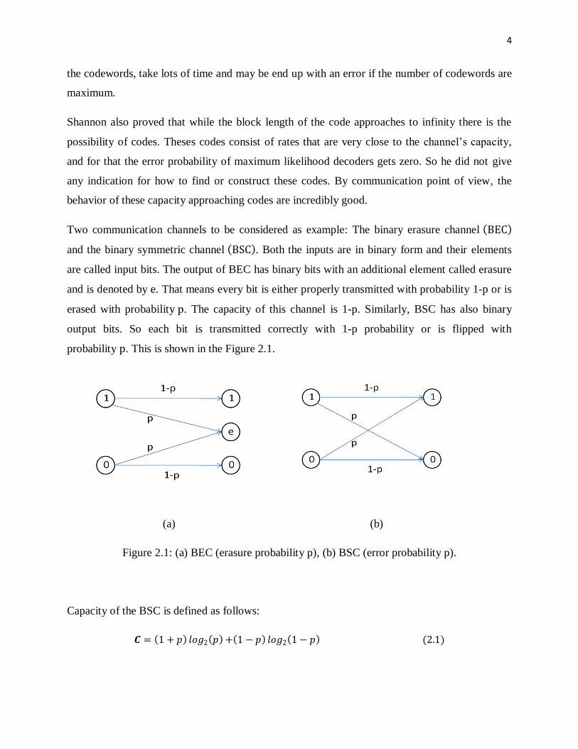
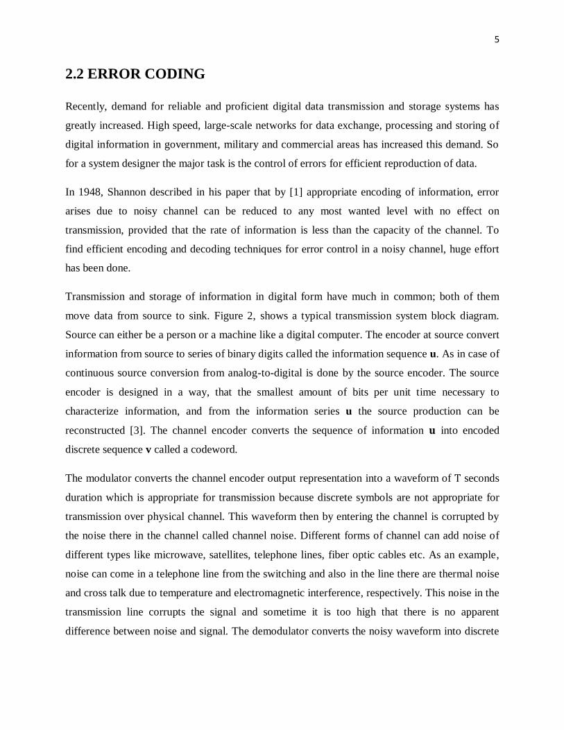
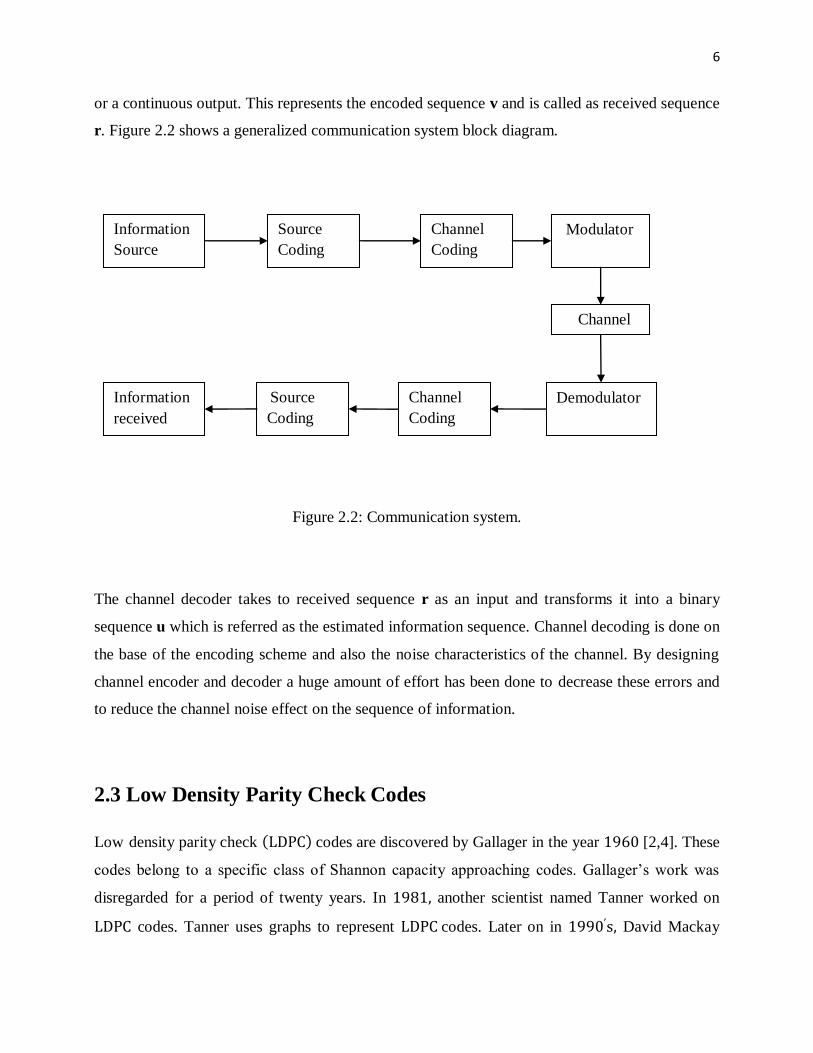


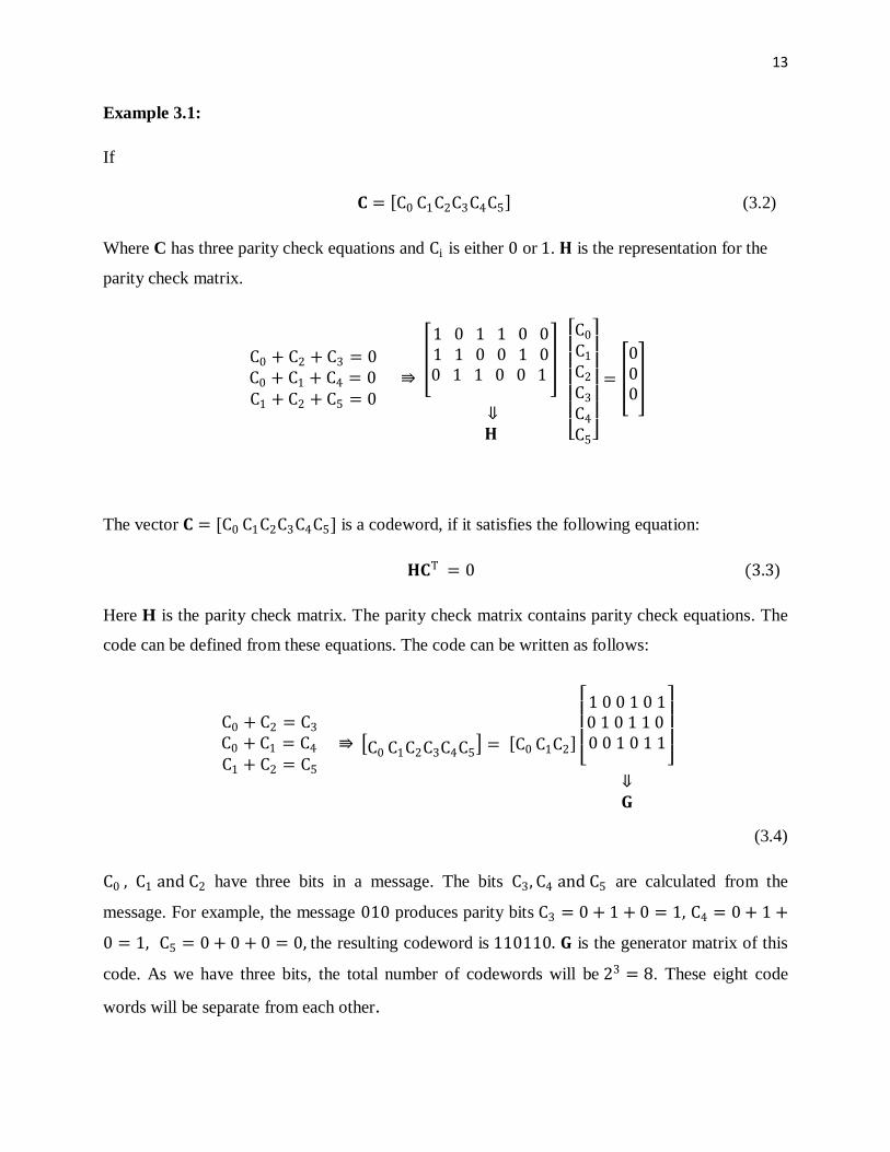

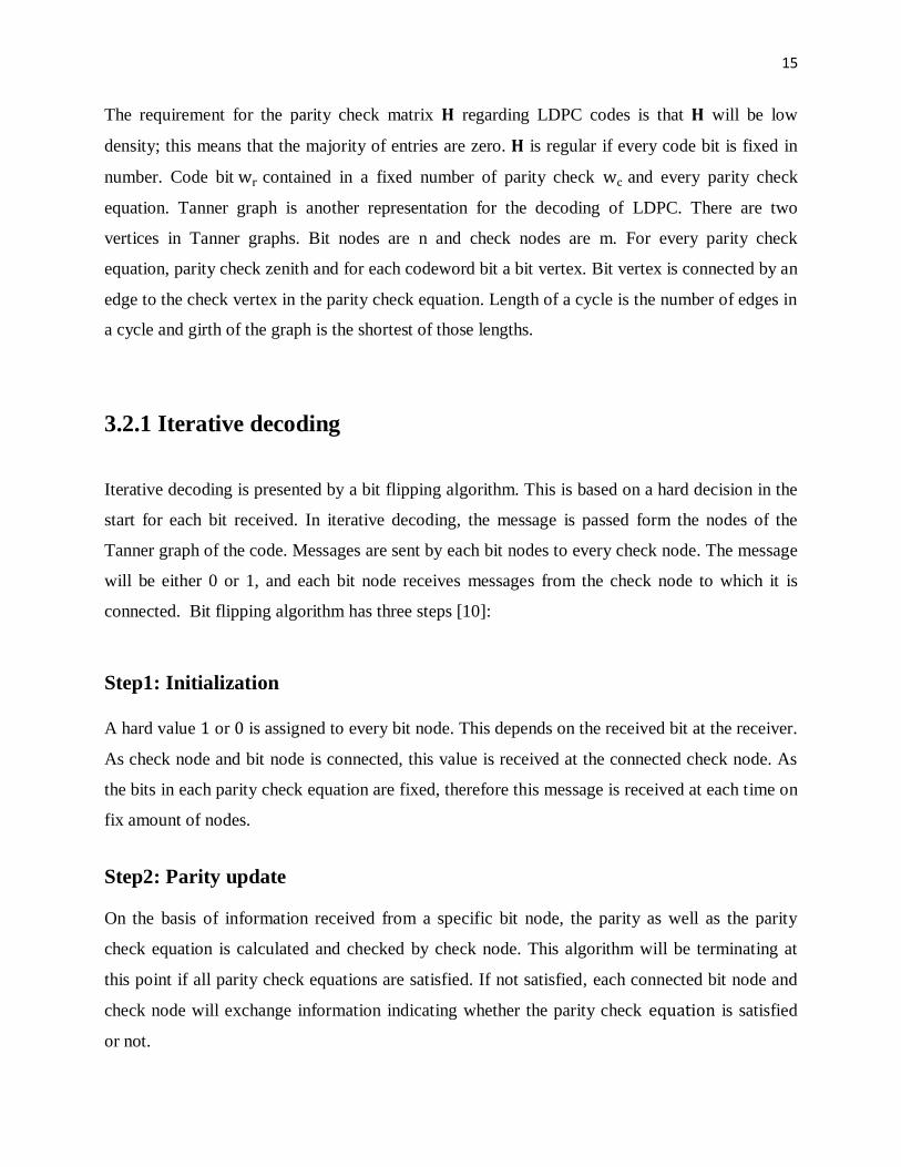
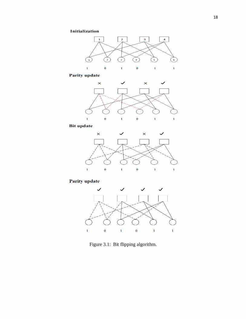

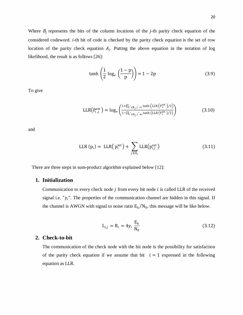
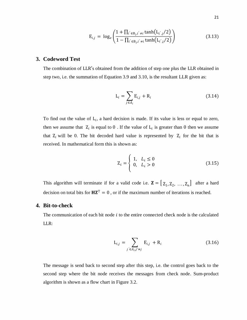


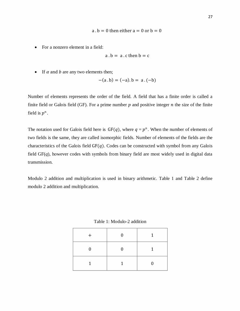
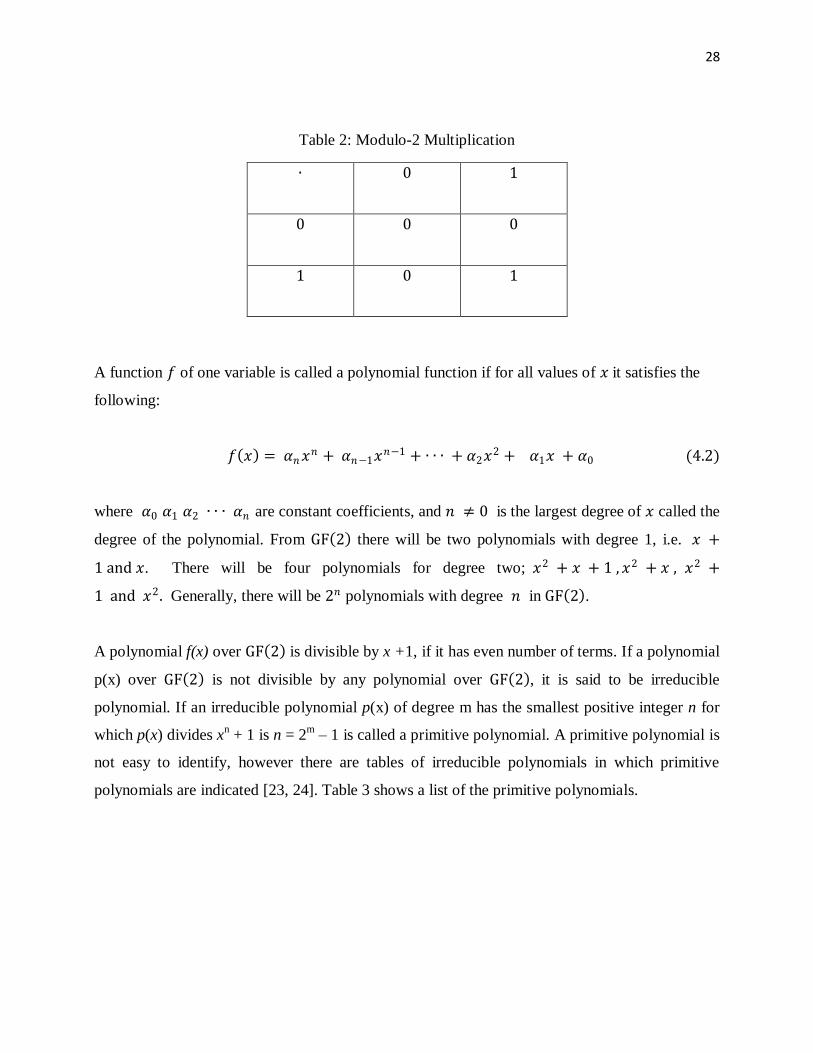
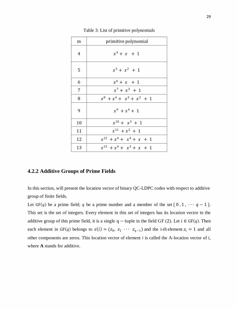
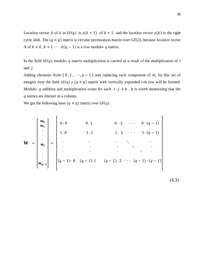
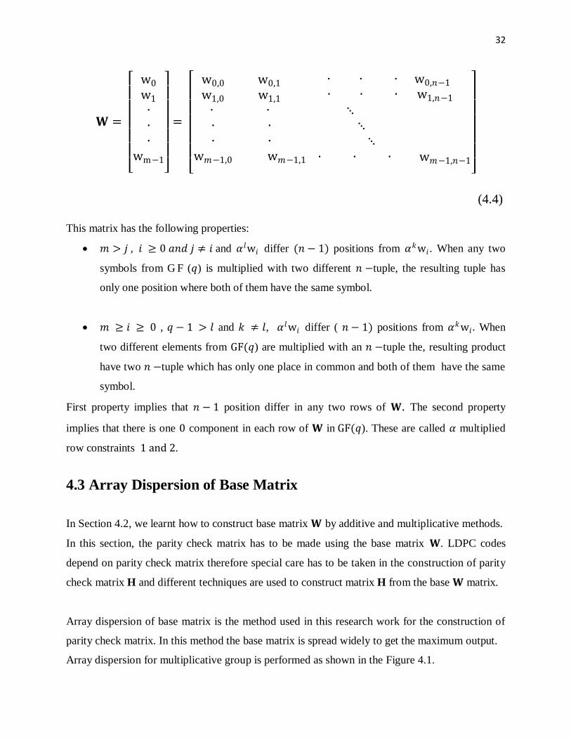
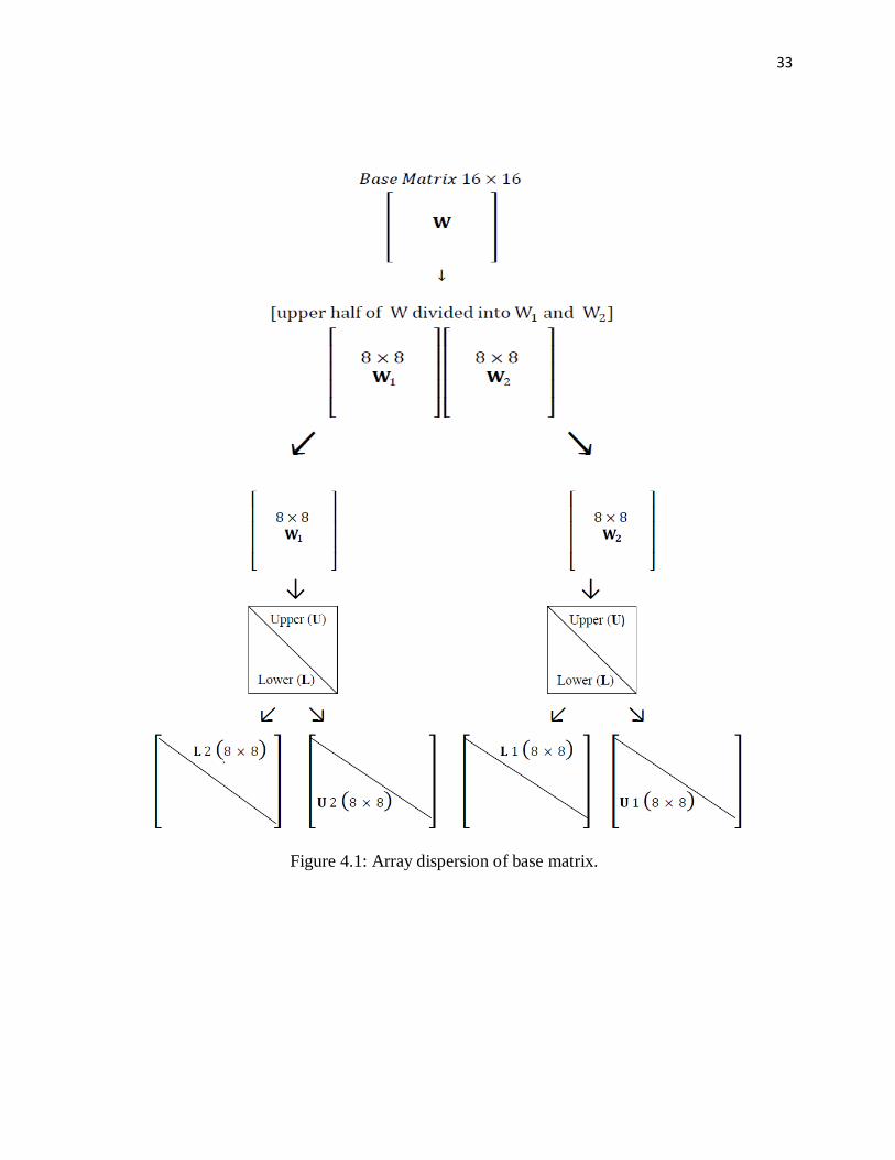
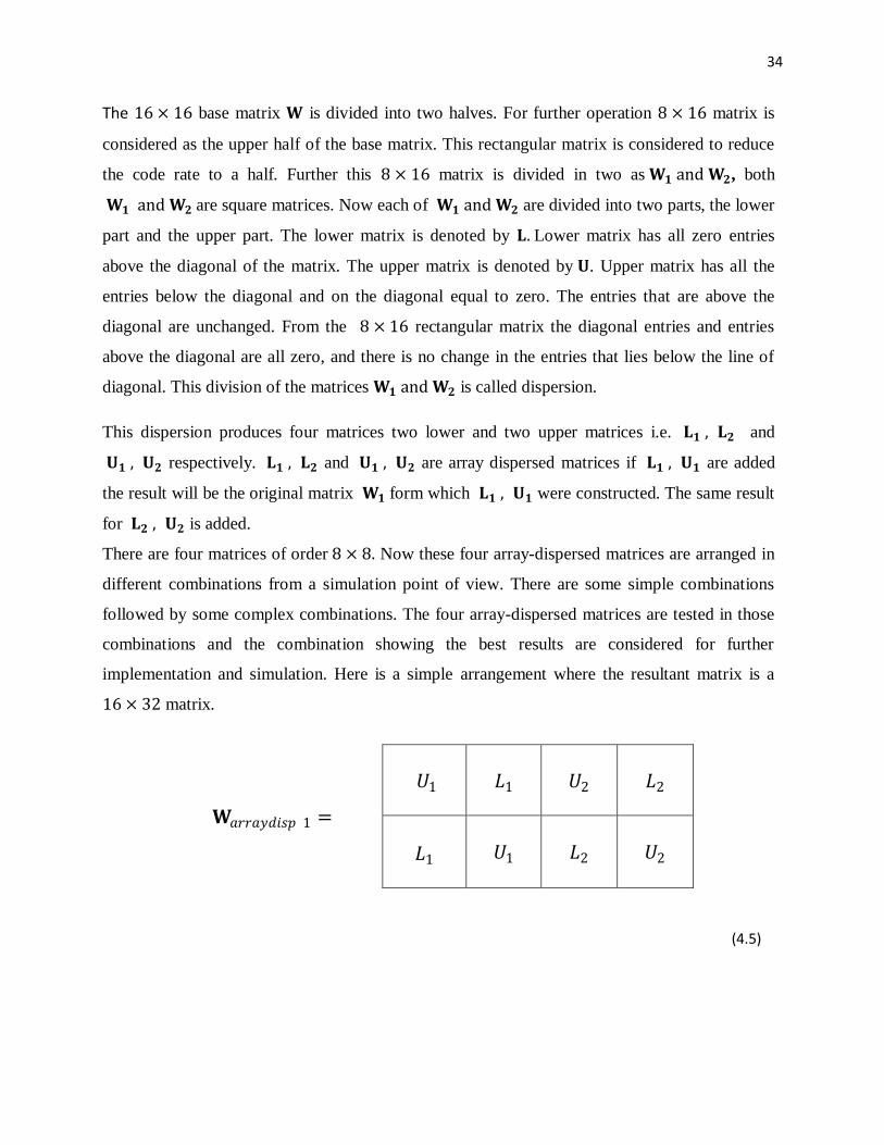
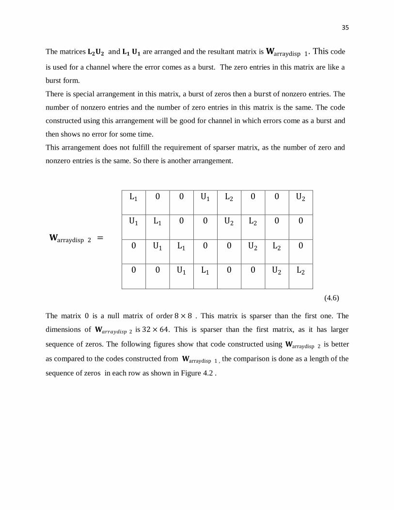
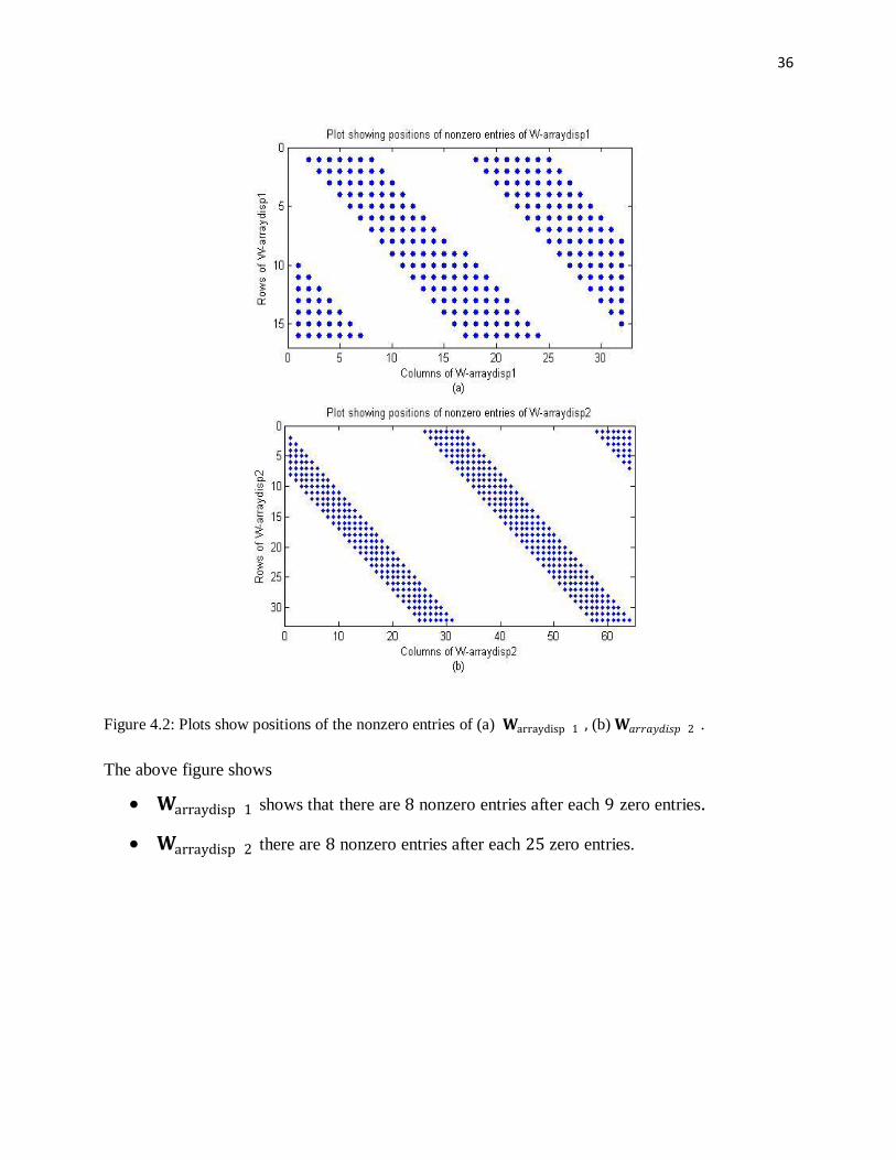

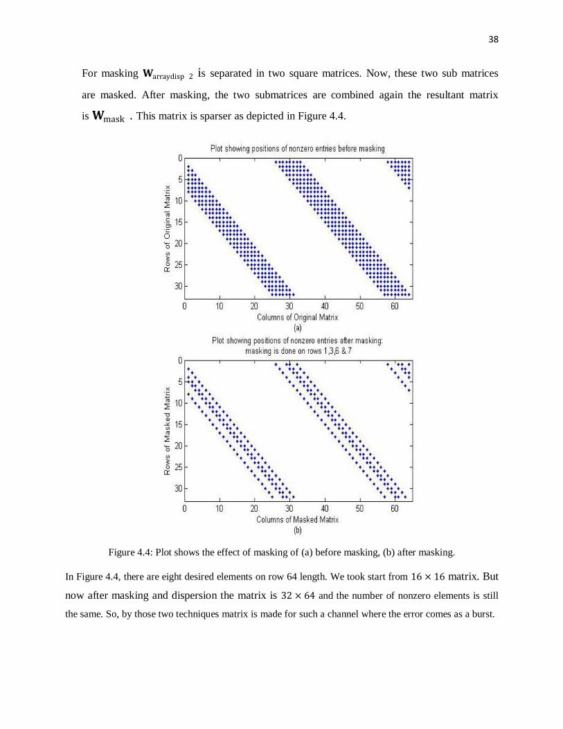
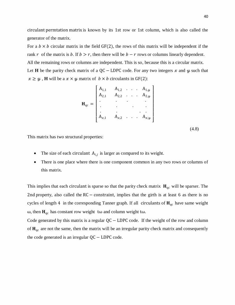
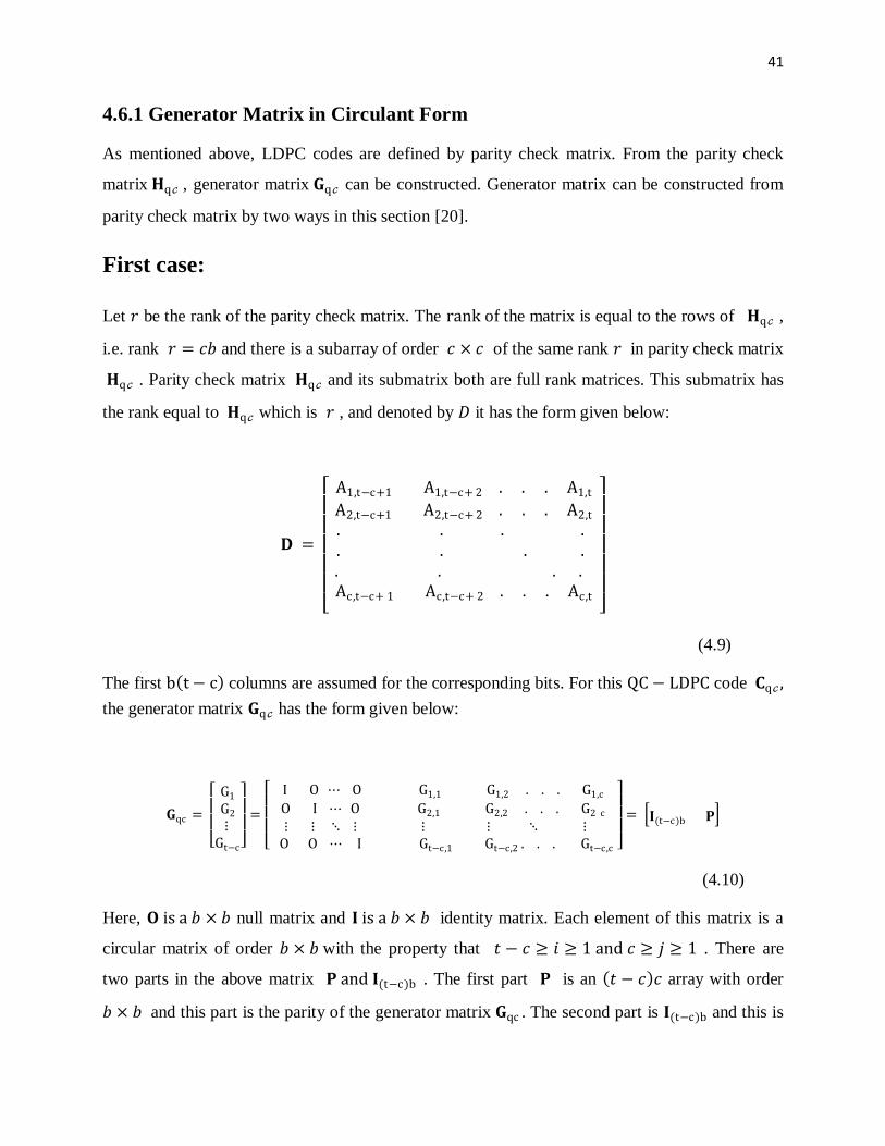
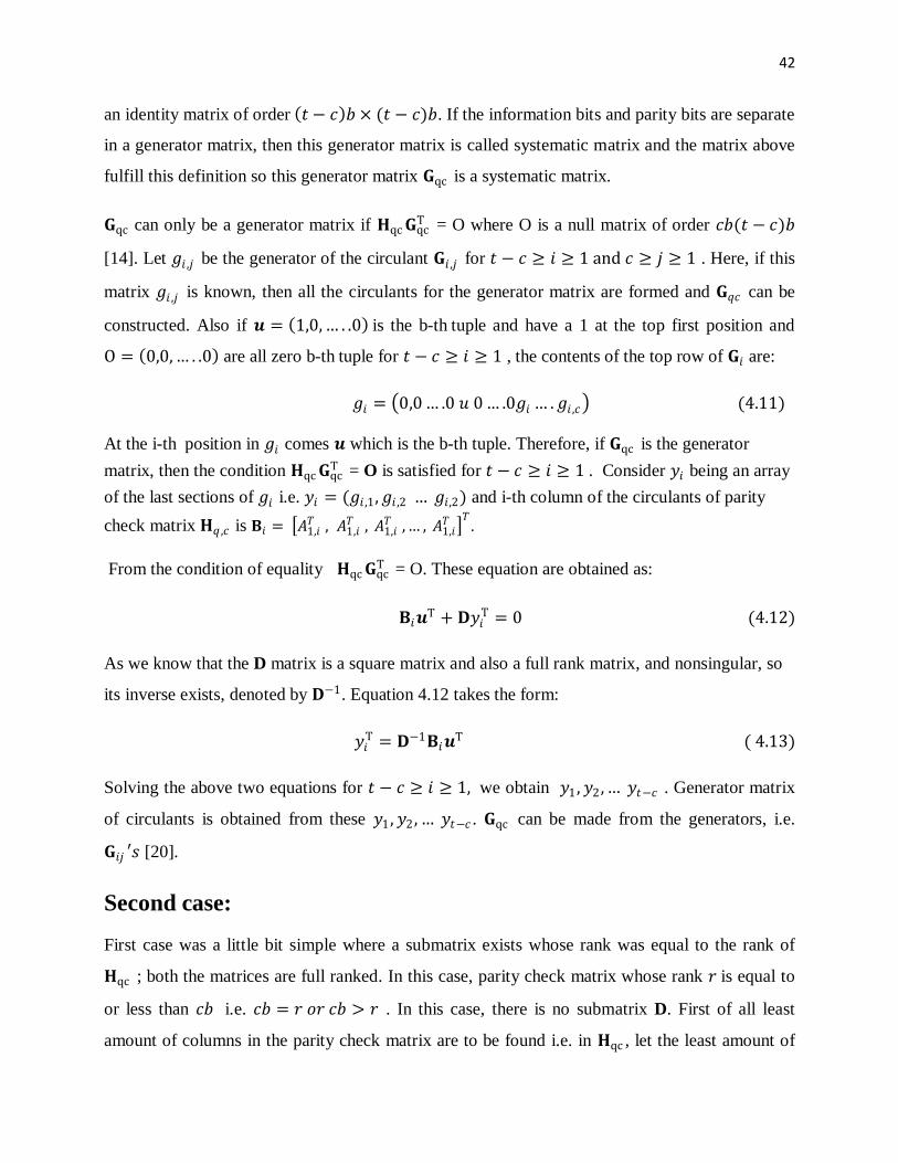

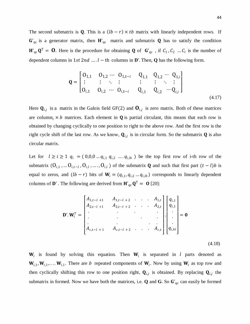
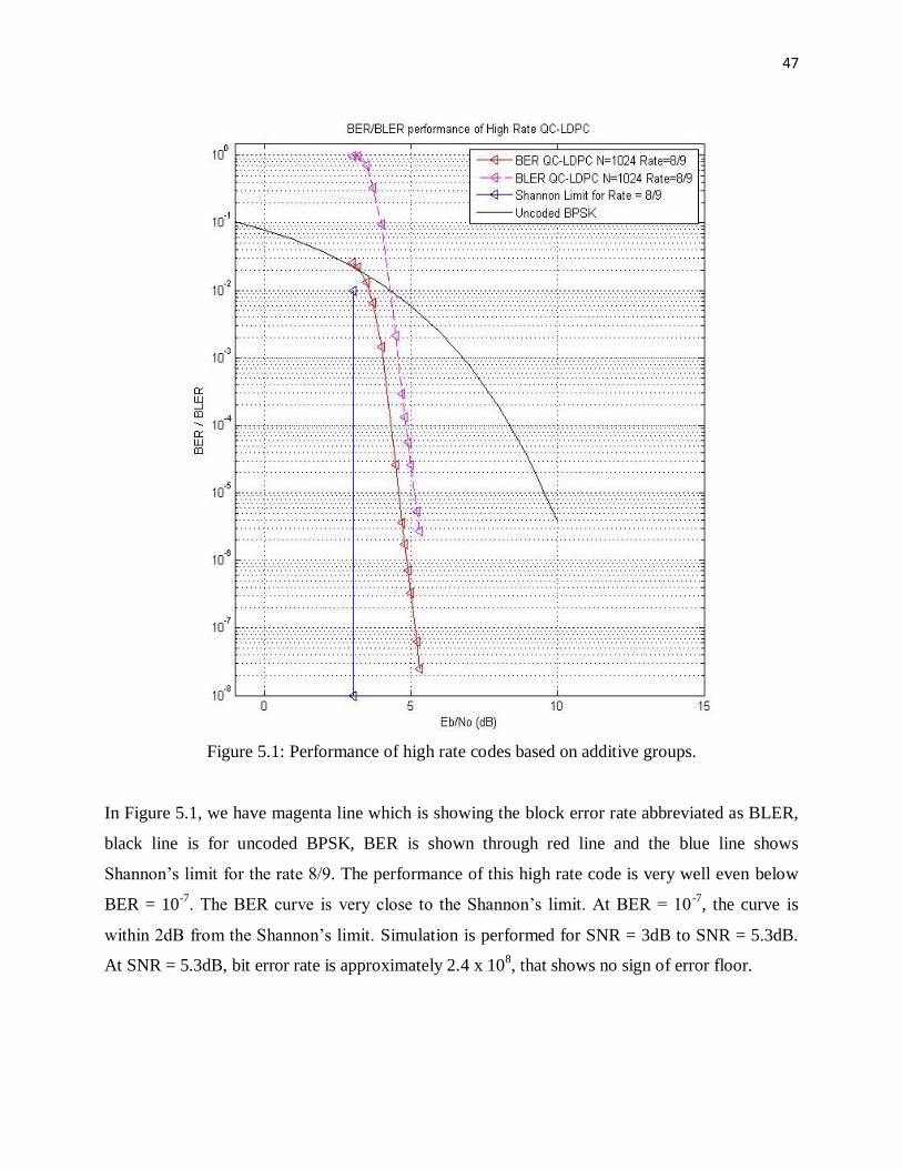
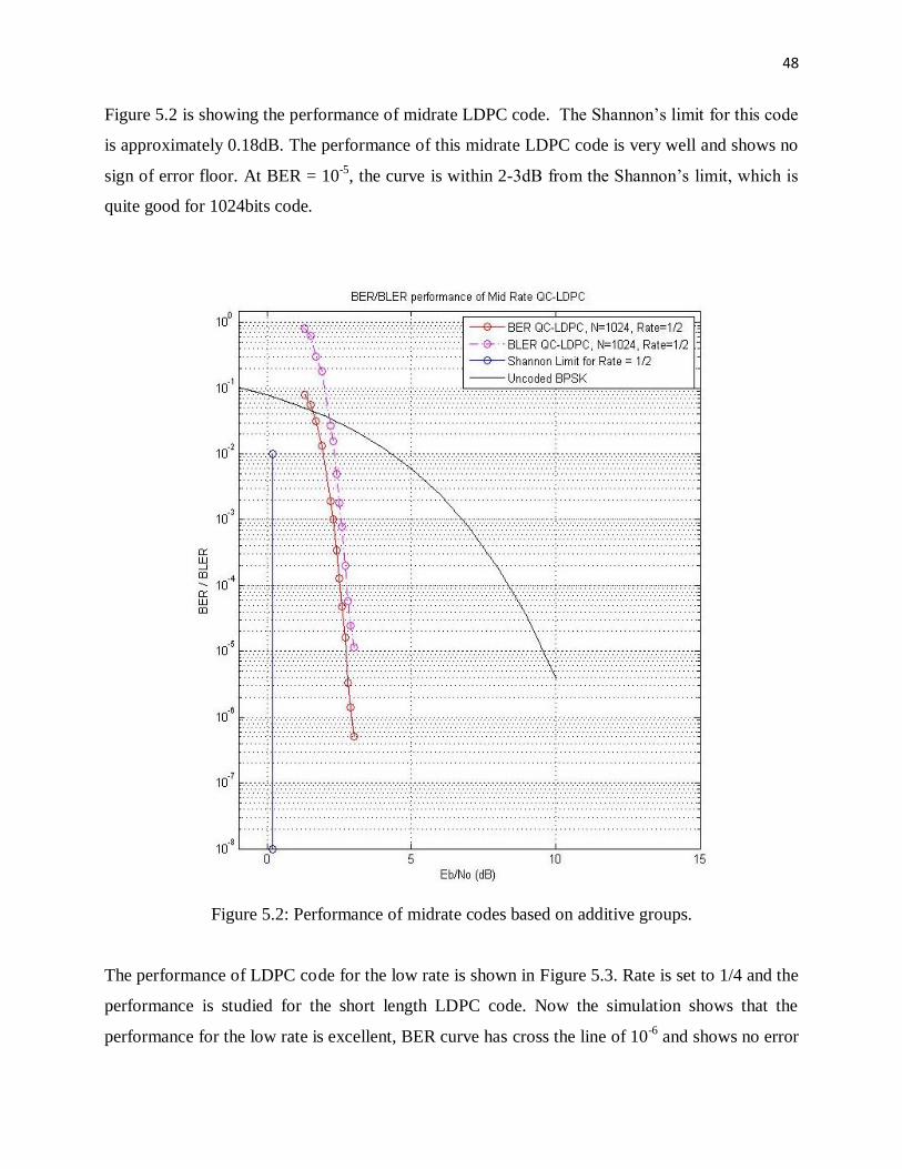
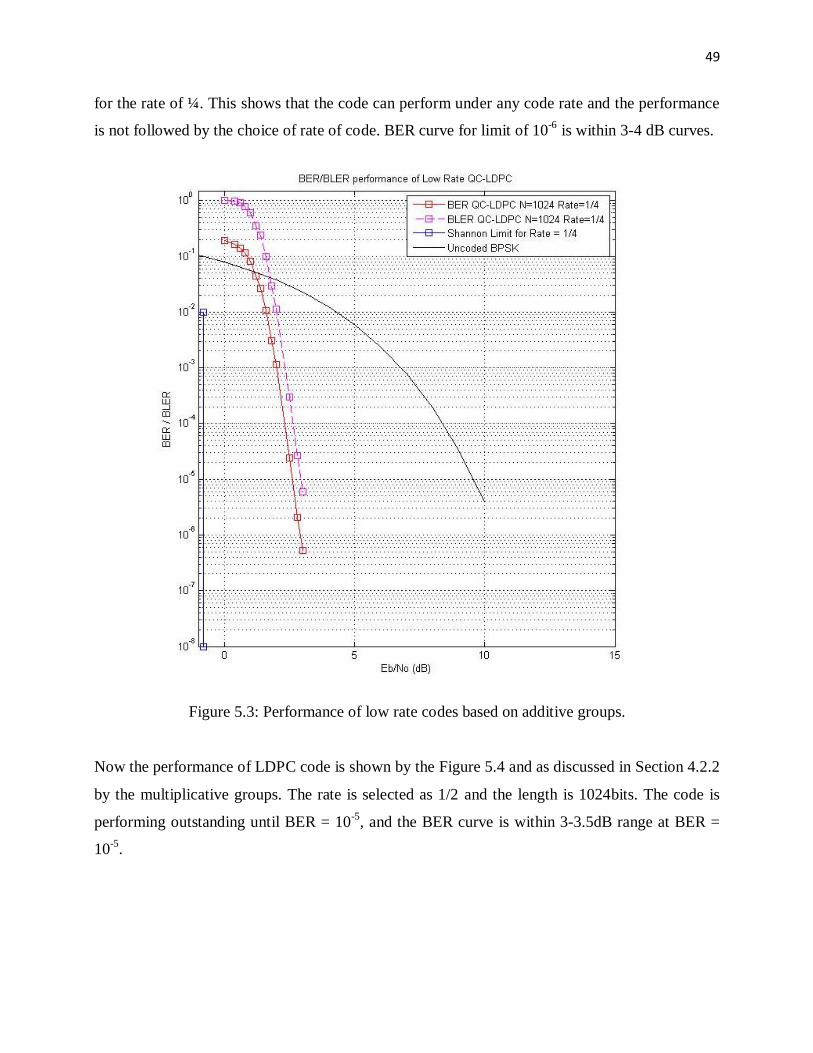
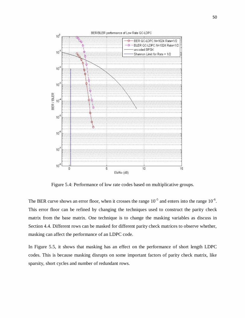


![Error Floor Approximation for LDPC Codes in the AWGN Channel · parity-check (LDPC) codes, was first published by Gal-lager in 1962 [1], [2]. LDPC codes are linear block codes de-scribed](https://static.documents.pub/doc/80x56/5e6fbd2513db9b54e934d6e6/error-floor-approximation-for-ldpc-codes-in-the-awgn-channel-parity-check-ldpc.jpg)
![Non-Binary Protograph-Based LDPC Codes: Analysis ...1.2 LDPC codes LDPC codes are a class of linear block codes invented by Gallager in his 1960 PhD the-sis [8]. Gallager noticed the](https://static.documents.pub/doc/80x56/6121a8a11cb8ce31dd153553/non-binary-protograph-based-ldpc-codes-analysis-12-ldpc-codes-ldpc-codes-are.jpg)


