65
CS 554m controlled experiments I Joanna McGrenere
CS 554m controlled experiments I
Joanna McGrenere
2
learning goals
be able to answer the following: what is the experimental method? what is an experimental hypothesis? how do I plan an experiment? why are statistics used? within- & between-subject comparisons: how do they differ? how do I compute a t-test? what are the different types of t-tests?
Acknowledgement: Some of the material in this lecture is based on material prepared for similar courses by Saul Greenberg (University of Calgary)

3
a good portion of the material in these lectures on experimental design should be familiar from ugrad stats class, although perhaps presented here from a slightly different perspective
also, most of this material is well covered in today’s readings:
Newman & Lamming, Ch 10
Lazar, Feng, & Hochheiser, Ch 2 - 4
Who has run an experiment?
4
5
material I assume you already know and will not be covered
(some additional slides at end) types of variables samples & populations normal distribution variance and standard deviation
6
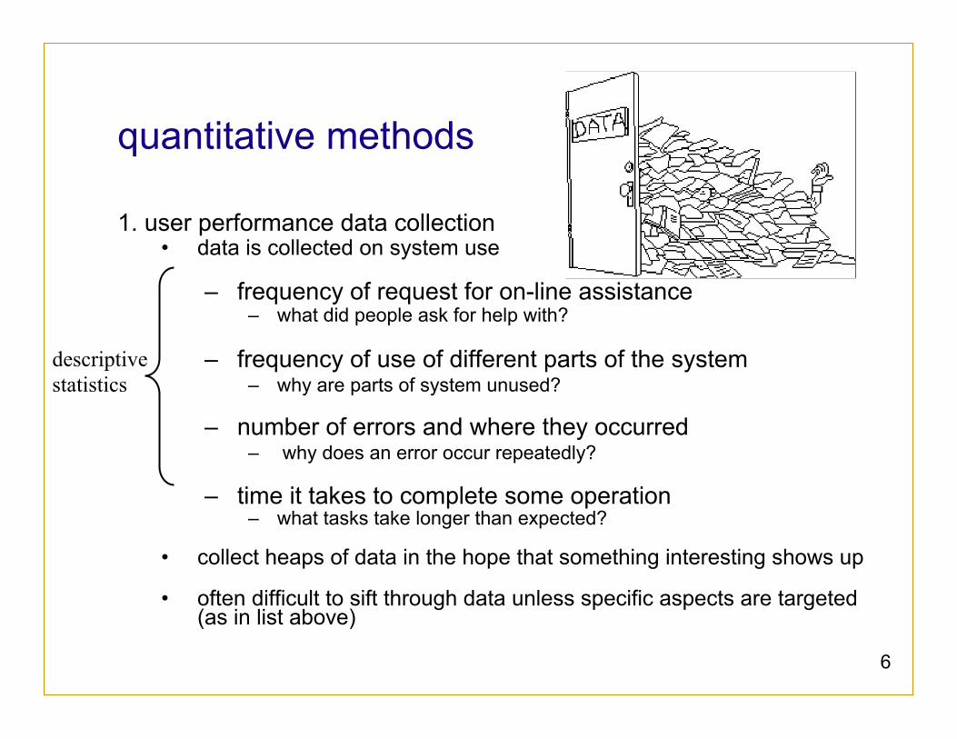
quantitative methods
1. user performance data collection • data is collected on system use
– frequency of request for on-line assistance
– what did people ask for help with?
– frequency of use of different parts of the system – why are parts of system unused?
– number of errors and where they occurred
– why does an error occur repeatedly?
– time it takes to complete some operation – what tasks take longer than expected?
• collect heaps of data in the hope that something interesting shows up
• often difficult to sift through data unless specific aspects are targeted
(as in list above)
descriptive statistics
7
quantitative methods
2. controlled experiments
the traditional scientific method • reductionist
– clear convincing result on specific issues • in HCI
– insights into cognitive process, human performance limitations, ... – allows comparison of systems, fine-tuning of details ...
strives for • lucid and testable hypothesis (usually a causal inference) • quantitative measurement • measure of confidence in results obtained (inferencial statistics) • replicability of experiment • control of variables and conditions • removal of experimenter bias
8
desired outcome of a controlled experiment
statistical inference of an event or situation’s probability:
“Design A is better <in some specific sense> than Design B”
or, Design A meets a target: “90% of incoming students who have web experience can
complete course registration within 30 minutes”
steps in the experimental method
10
step 1: begin with a lucid, testable hypothesis
Example 1: H0: there is no difference in the number of cavities in children and
teenagers using crest and no-teeth toothpaste H1: children and teenagers using crest toothpaste have fewer
cavities than those who use no-teeth toothpaste
11
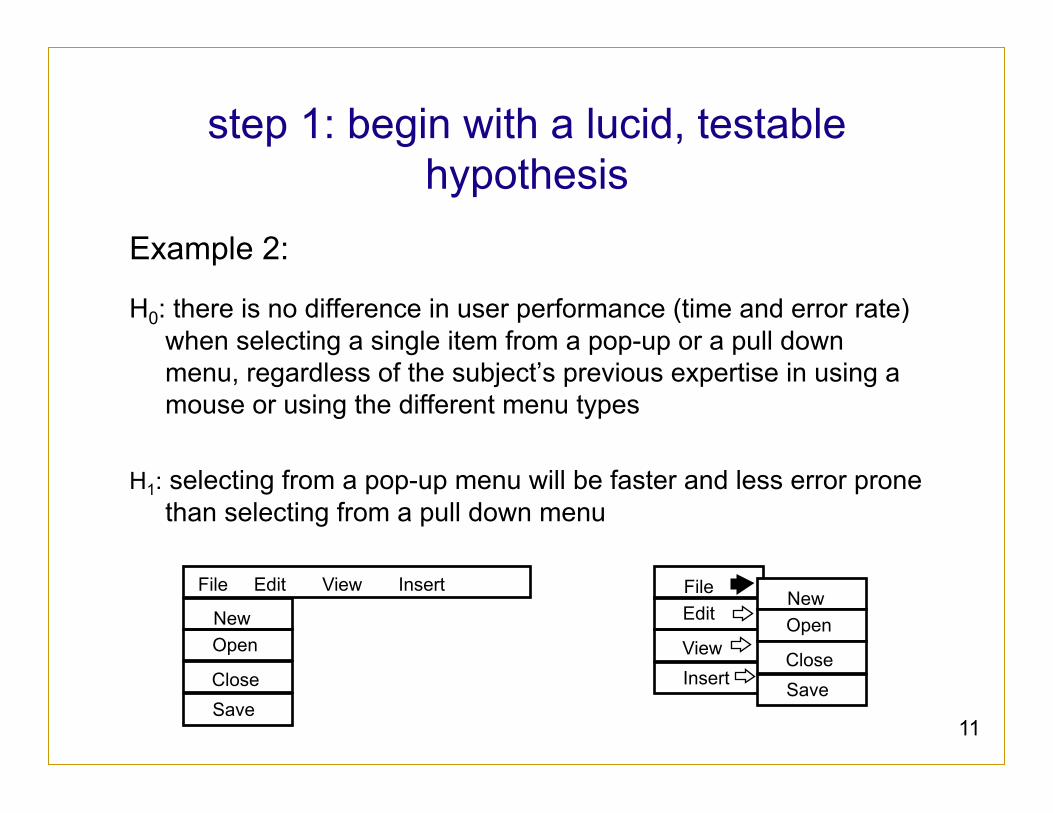
step 1: begin with a lucid, testable hypothesis
Example 2:
H0: there is no difference in user performance (time and error rate) when selecting a single item from a pop-up or a pull down menu, regardless of the subject’s previous expertise in using a mouse or using the different menu types
H1: selecting from a pop-up menu will be faster and less error prone
than selecting from a pull down menu
File Edit View Insert
New Open
Close Save
File Edit
View Insert
New Open
Close Save
12
general: hypothesis testing
hypothesis = prediction of the outcome of an experiment.
framed in terms of independent and dependent variables: a variation in the independent variable will cause a difference in the dependent variable.
aim of the experiment: prove this prediction do by: disproving the “null hypothesis”
H0: experimental conditions have no effect on performance (to some degree of significance) à null hypothesis
H1: experimental conditions have an effect on performance (to some degree of significance) à alternate hypothesis
13
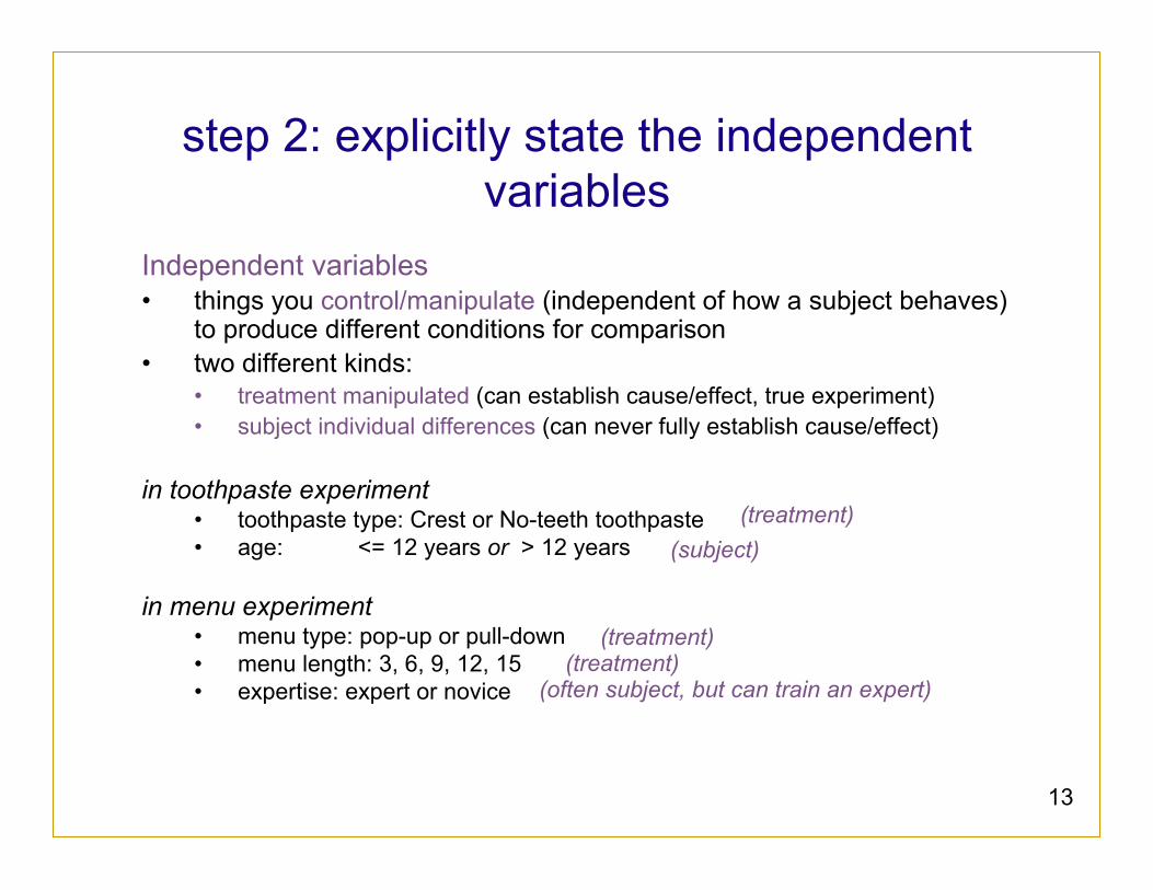
step 2: explicitly state the independent variables
Independent variables • things you control/manipulate (independent of how a subject behaves)
to produce different conditions for comparison • two different kinds:
• treatment manipulated (can establish cause/effect, true experiment) • subject individual differences (can never fully establish cause/effect)
in toothpaste experiment
• toothpaste type: Crest or No-teeth toothpaste • age: <= 12 years or > 12 years
in menu experiment
• menu type: pop-up or pull-down • menu length: 3, 6, 9, 12, 15 • expertise: expert or novice
(treatment)
(treatment) (treatment)
(subject)
(often subject, but can train an expert)
14
step 3: carefully choose the dependent variables
Dependent variables • things that are measured • expectation that they depend on the subject’s behaviour / reaction to
the independent variable (but unaffected by other factors)
in toothpaste experiment:
in menu experiment:
15
step 4: consider possible nuisance variables & determine mitigation approach • undesired variations in experiment conditions which cannot be
eliminated, but which may affect dependent variable – critical to know about them
• experiment design & analysis must generally accommodate them: – treat as an additional experiment independent variable (if they can
be controlled) – randomization (if they cannot be controlled)
• common nuisance variable: subject (individual differences) in toothpaste experiment:
in menu experiment:
how to manage?
16
step 5: design the task to be performed tasks must: be externally valid
external validity = do the results generalize? … will they be an accurate predictor of how well users can perform tasks as they would in real life? for a large interactive system, can probably only test a small subset of all possible tasks.
exercise the designs, bringing out any differences in their support for the task
e.g., if a design supports website navigation, test task should not require subject to work within a single page
be feasible - supported by the design/prototype, and executable within experiment time scale
17
step 5: design the task to be performed in toothpaste experiment:
in menu experiment:
18
step 6: design experiment protocol
• steps for executing experiment are prepared well ahead of time • includes unbiased instructions + instruments (questionnaire,
interview script, observation sheet) • double-blind experiments, ...
Now you get to do the pop-up menus. I think you will really like them... I designed them myself!
19
step 7: make formal experiment design explicit
simplest: 2-sample (2-condition) experiment based on comparison of two sample means: • performance data from using Design A & Design B
– e.g., new design & status quo design – e.g., 2 new designs
or, comparison of one sample mean with a constant: • performance data from using Design A, compared to
performance requirement – determine whether single new design meets key design
requirement
20
step 7: make formal experiment design explicit
more complex: factorial design in toothpaste experiment:
2 toothpaste types (crest, no-teeth) x 2 age groups (<= 12 years or > 12 years)
in menu experiment:
2 menu types (pop-up, pull down) x 5 menu lengths (3, 6, 9, 12, 15) x 2 levels of expertise (novice, expert)
21
step 8: judiciously select/recruit and assign subjects to groups
subject pool: similar issues as for informal studies • match expected user population as closely as possible • age, physical attributes, level of education • general experience with systems similar to those being tested • experience and knowledge of task domain
sample size: more critical in experiments than informal studies • going for “statistical significance” • should be large enough to be “representative” of population • guidelines exist based on statistical methods used & required
significance of results • pragmatic concerns may dictate actual numbers • “10” is often a good place to start
22
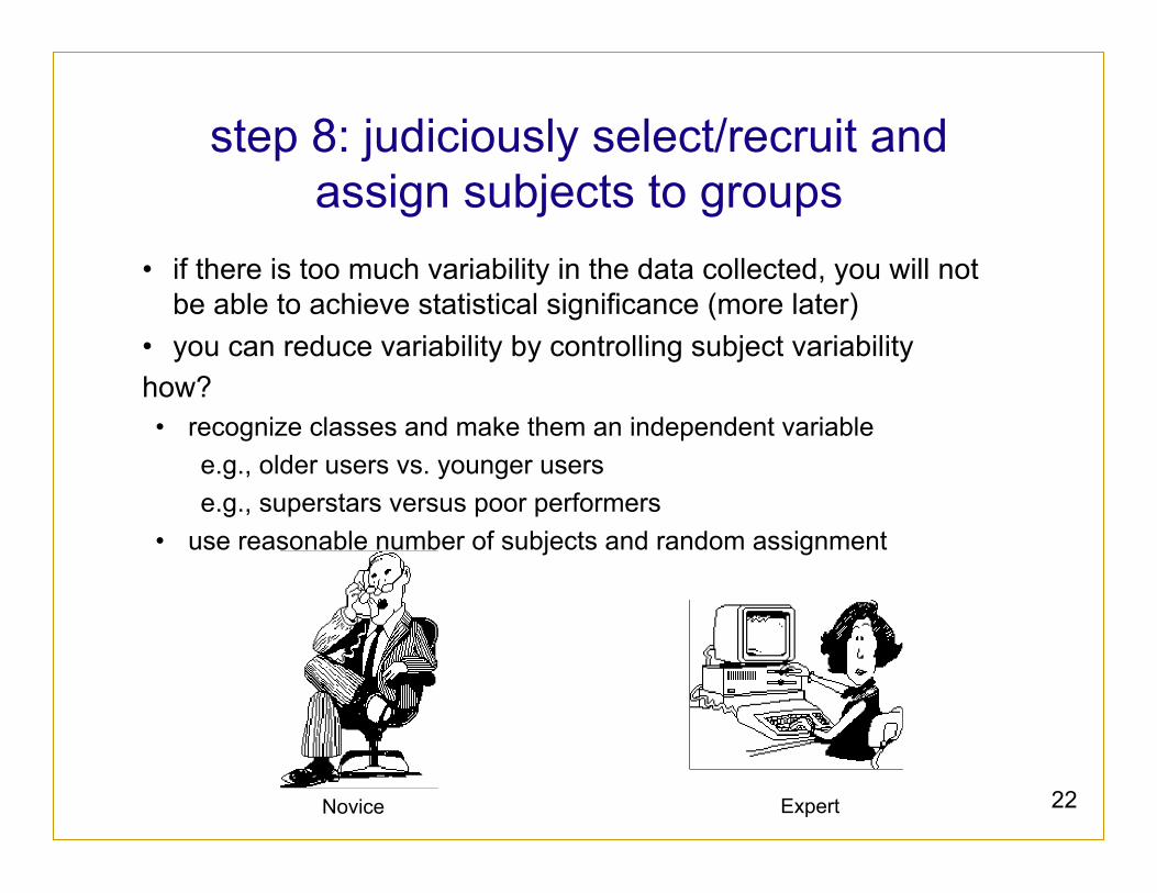
step 8: judiciously select/recruit and assign subjects to groups
• if there is too much variability in the data collected, you will not be able to achieve statistical significance (more later)
• you can reduce variability by controlling subject variability how? • recognize classes and make them an independent variable
e.g., older users vs. younger users e.g., superstars versus poor performers
• use reasonable number of subjects and random assignment
Novice Expert
23
step 9: apply statistical methods to data analysis
examples: t-tests, ANOVA, correlation, regression (more on these later) confidence limits: the confidence that your conclusion is correct
– “The hypothesis that mouse experience makes no difference is rejected at the .05 level” (i.e., null hypothesis rejected)
– this means: – a 95% chance that your finding is correct – a 5% chance you are wrong
24
step 10: interpret your results
what you believe the results mean, and their implications yes, there can be a subjective component to quantitative analysis
25
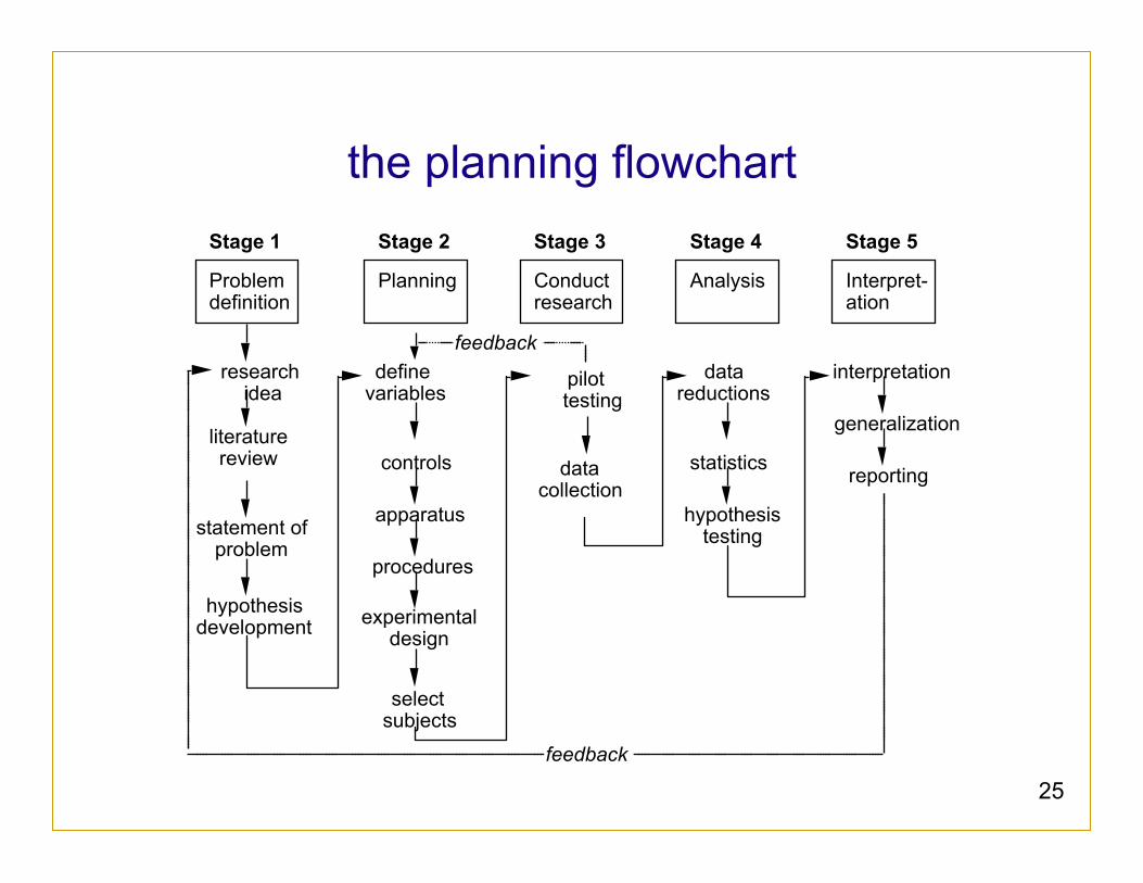
the planning flowchart Stage 1
Problem definition
research idea
literature review
statement of problem
hypothesis development
Stage 2
Planning
define variables
controls
apparatus
procedures
Stage 3
Conduct research
data collection
Stage 4
Analysis
data reductions
statistics
hypothesis testing
Stage 5
Interpret- ation
interpretation
generalization
reporting
select subjects
experimental design
pilot testing
feedback
feedback
26
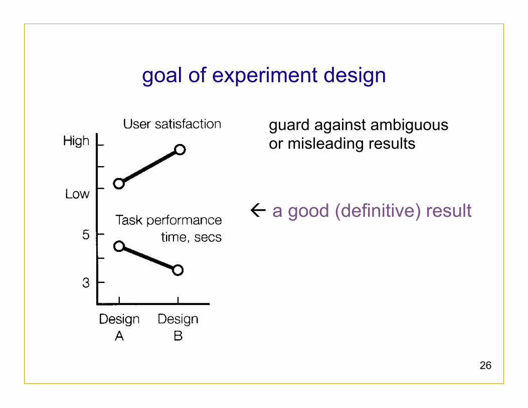
goal of experiment design
guard against ambiguous or misleading results
ß a good (definitive) result
27
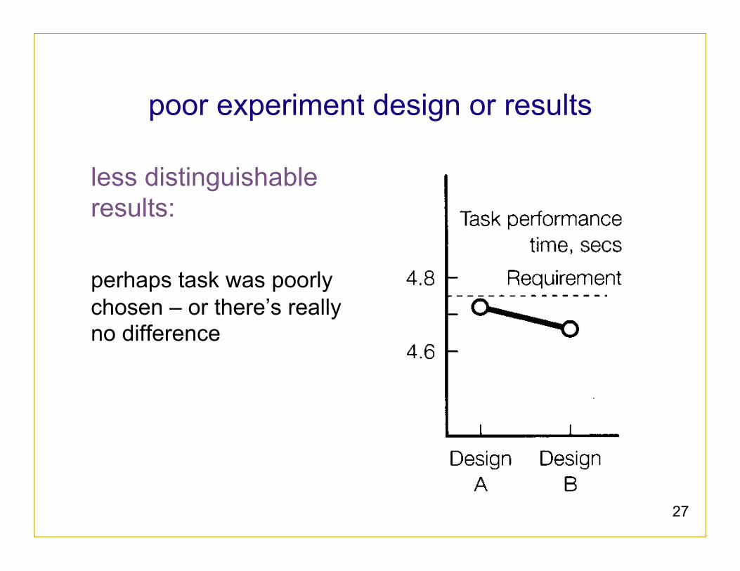
poor experiment design or results
less distinguishable results: perhaps task was poorly chosen – or there’s really no difference
28
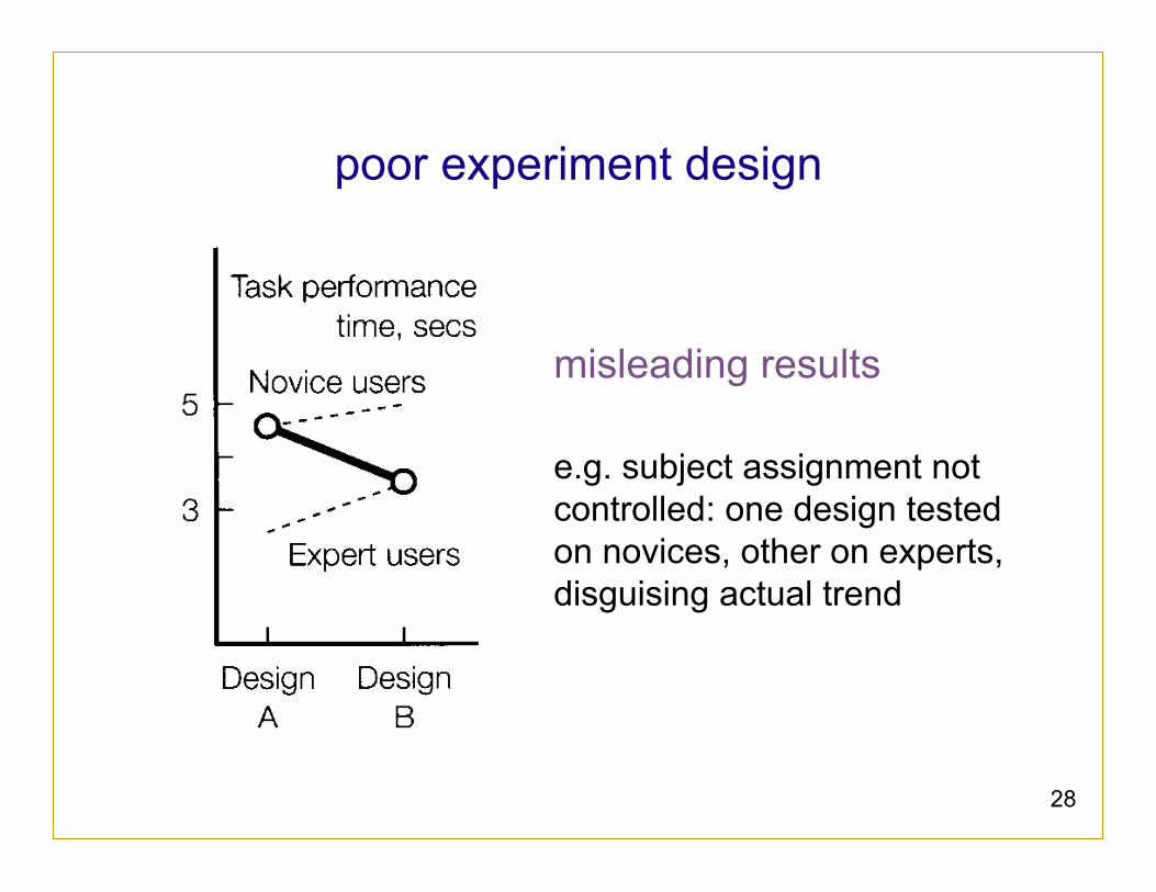
poor experiment design
misleading results e.g. subject assignment not controlled: one design tested on novices, other on experts, disguising actual trend
29
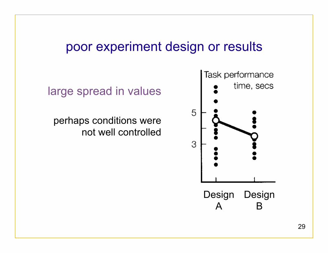
poor experiment design or results
large spread in values
perhaps conditions were not well controlled
Design A
Design B
30
as we have seen
individual (subject) differences may pose a nuisance variable:
variation in individual abilities can mask real differences in test conditions, if not analyzed properly
31
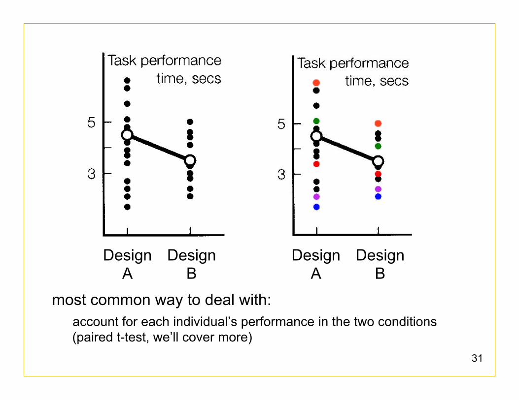
most common way to deal with: account for each individual’s performance in the two conditions (paired t-test, we’ll cover more)
Design A
Design B
Design A
Design B
32
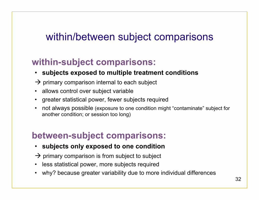
within/between subject comparisons
within-subject comparisons: • subjects exposed to multiple treatment conditions à primary comparison internal to each subject • allows control over subject variable • greater statistical power, fewer subjects required • not always possible (exposure to one condition might “contaminate” subject for
another condition; or session too long)
between-subject comparisons: • subjects only exposed to one condition à primary comparison is from subject to subject • less statistical power, more subjects required • why? because greater variability due to more individual differences
in toothpaste experiment 2 toothpaste types (crest, no-teeth) x 2 age groups (<= 12 years or > 12 years)
in menu experiment :
2 menu types (pop-up, pull down) x 5 menu lengths (3, 6, 9, 12, 15) x 2 levels of expertise (novice, expert)
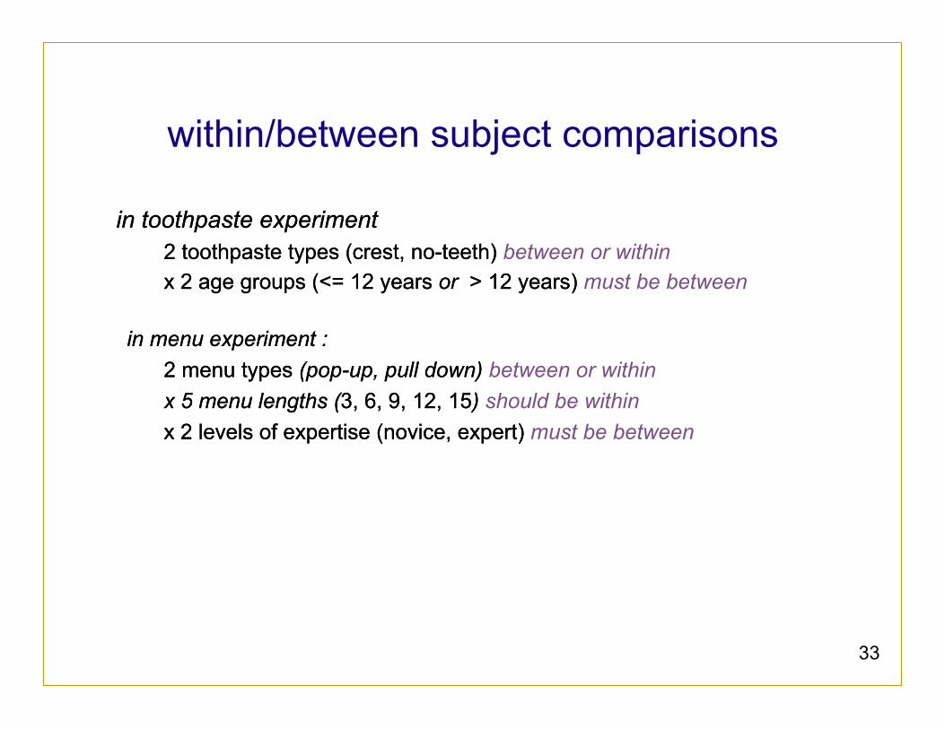
in toothpaste experiment 2 toothpaste types (crest, no-teeth) between or within x 2 age groups (<= 12 years or > 12 years) must be between
in menu experiment :
2 menu types (pop-up, pull down) between or within x 5 menu lengths (3, 6, 9, 12, 15) should be within x 2 levels of expertise (novice, expert) must be between
33
within/between subject comparisons
34
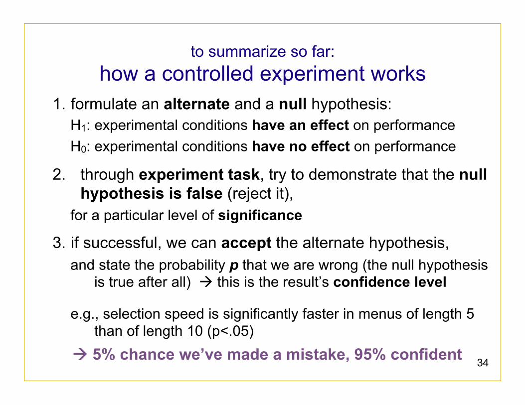
to summarize so far: how a controlled experiment works
1. formulate an alternate and a null hypothesis: H1: experimental conditions have an effect on performance H0: experimental conditions have no effect on performance
2. through experiment task, try to demonstrate that the null hypothesis is false (reject it),
for a particular level of significance
3. if successful, we can accept the alternate hypothesis, and state the probability p that we are wrong (the null hypothesis
is true after all) à this is the result’s confidence level
e.g., selection speed is significantly faster in menus of length 5 than of length 10 (p<.05)
à 5% chance we’ve made a mistake, 95% confident
35
statistical analysis what is a statistic? • a number that describes a sample • sample is a subset (hopefully representative) of the population we are
interested in understanding
statistics are calculations that tell us • mathematical attributes about our data sets (sample)
– mean, amount of variance, ...
• how data sets relate to each other – whether we are “sampling” from the same or different populations
• the probability that our claims are correct
– “statistical significance”
36
example: differences between means
given: two data sets measuring a condition • e.g., height difference of males and females,
time to select an item from different menu styles ... question: • is the difference between the means of the data statistically
significant?
null hypothesis: • there is no difference between the two means • statistical analysis can only reject the hypothesis at a certain
level of confidence • note: we never actually prove the null hypothesis true
37
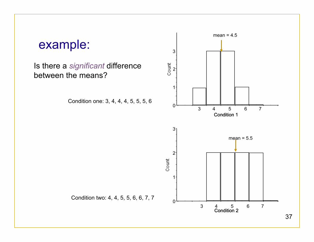
example: Is there a significant difference between the means?
Condition one: 3, 4, 4, 4, 5, 5, 5, 6
Condition two: 4, 4, 5, 5, 6, 6, 7, 7
0
1
2
3
Condition 1 Condition 1
0
1
2
3
Condition 2 Condition 2
3 4 5 6 7
mean = 4.5
mean = 5.5
3 4 5 6 7
38
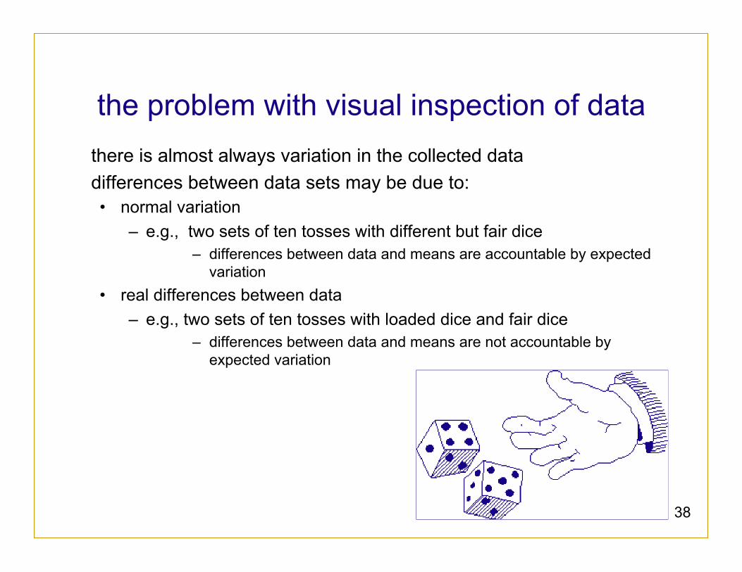
the problem with visual inspection of data there is almost always variation in the collected data differences between data sets may be due to: • normal variation
– e.g., two sets of ten tosses with different but fair dice – differences between data and means are accountable by expected
variation • real differences between data
– e.g., two sets of ten tosses with loaded dice and fair dice – differences between data and means are not accountable by
expected variation
39
t-test
a statistical test allows one to say something about differences between two means at a certain confidence level null hypothesis of the t-test:
no difference exists between the means possible results: • I am 95% sure that null hypothesis is rejected
– there is probably a true difference between the means
• I cannot reject the null hypothesis – the means are likely the same
40
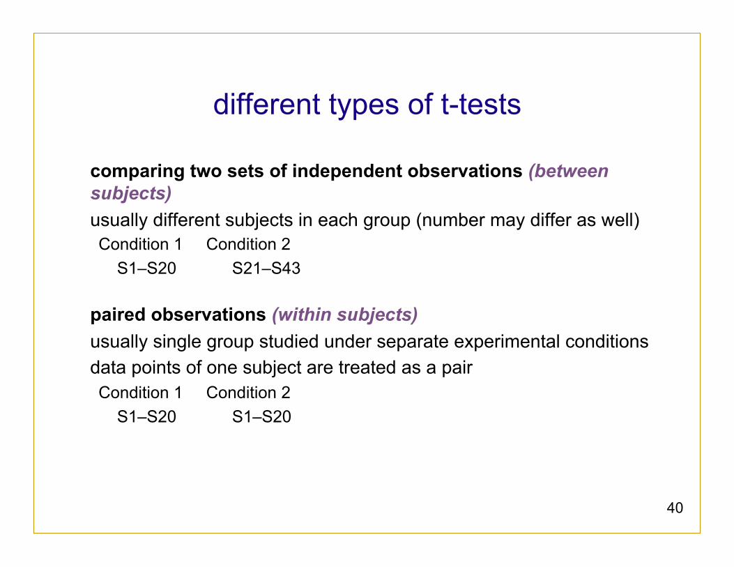
different types of t-tests
comparing two sets of independent observations (between subjects) usually different subjects in each group (number may differ as well) Condition 1 Condition 2 S1–S20 S21–S43
paired observations (within subjects) usually single group studied under separate experimental conditions data points of one subject are treated as a pair Condition 1 Condition 2 S1–S20 S1–S20
41
different types of t-tests
non-directional vs directional alternatives non-directional (two-tailed) • no expectation that the direction of difference matters
directional (one-tailed) • only interested if the mean of a given condition is greater than the
other
42
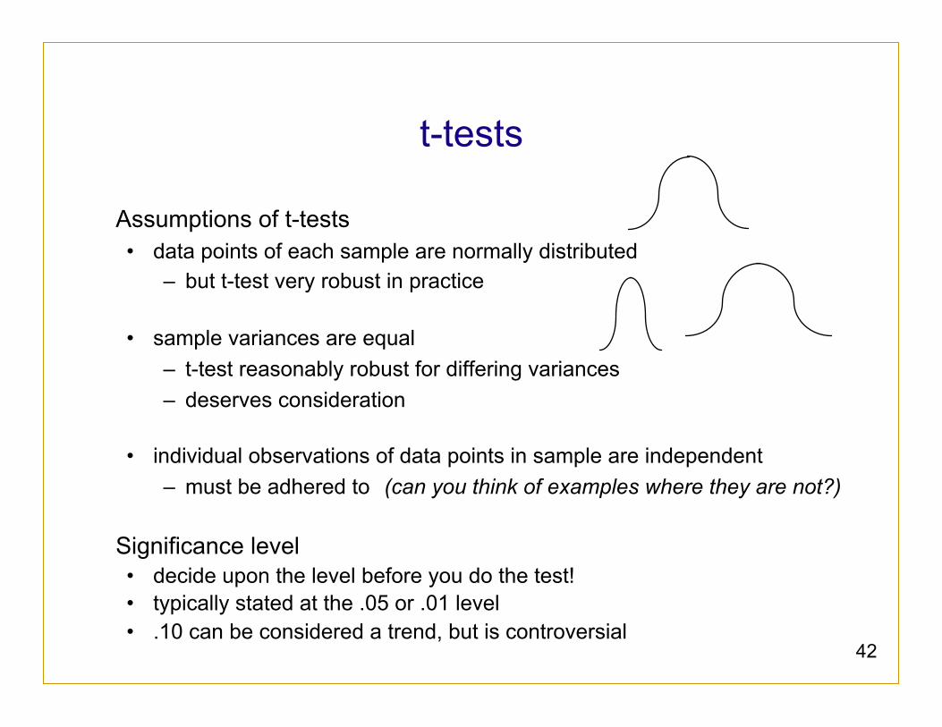
t-tests
Assumptions of t-tests • data points of each sample are normally distributed
– but t-test very robust in practice
• sample variances are equal – t-test reasonably robust for differing variances – deserves consideration
• individual observations of data points in sample are independent
– must be adhered to (can you think of examples where they are not?)
Significance level • decide upon the level before you do the test! • typically stated at the .05 or .01 level • .10 can be considered a trend, but is controversial
43
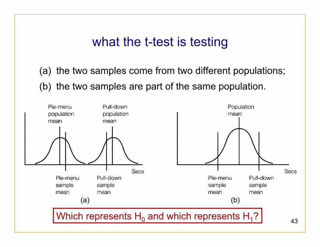
what the t-test is testing
(a) the two samples come from two different populations; (b) the two samples are part of the same population.
(a) (b)
Which represents H0 and which represents H1?
44
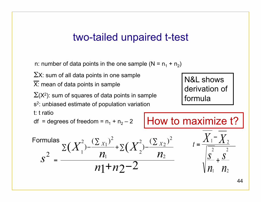
two-tailed unpaired t-test
n: number of data points in the one sample (N = n1 + n2)
ΣX: sum of all data points in one sample X: mean of data points in sample
Σ(X2): sum of squares of data points in sample s2: unbiased estimate of population variation t: t ratio df = degrees of freedom = n1 + n2 – 2 Formulas
221
((2
222
21
212
1
)()
)()
2
−+
∑−∑+
∑−∑
=nn
nXnXs
XX
ns
nsXXt
2
2
1
221
+
−=
N&L shows derivation of formula
How to maximize t?
45
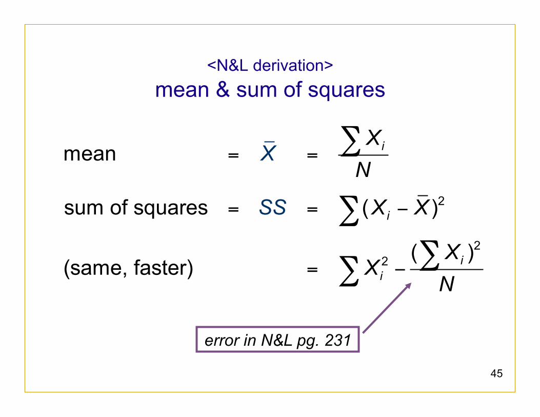
<N&L derivation> mean & sum of squares
= =
= = −
= −
∑
∑
∑∑
2
22
mean
sum of squares ( )
( )(same, faster)
i
i
ii
XN
X X
XX
X
S
N
S
error in N&L pg. 231
46
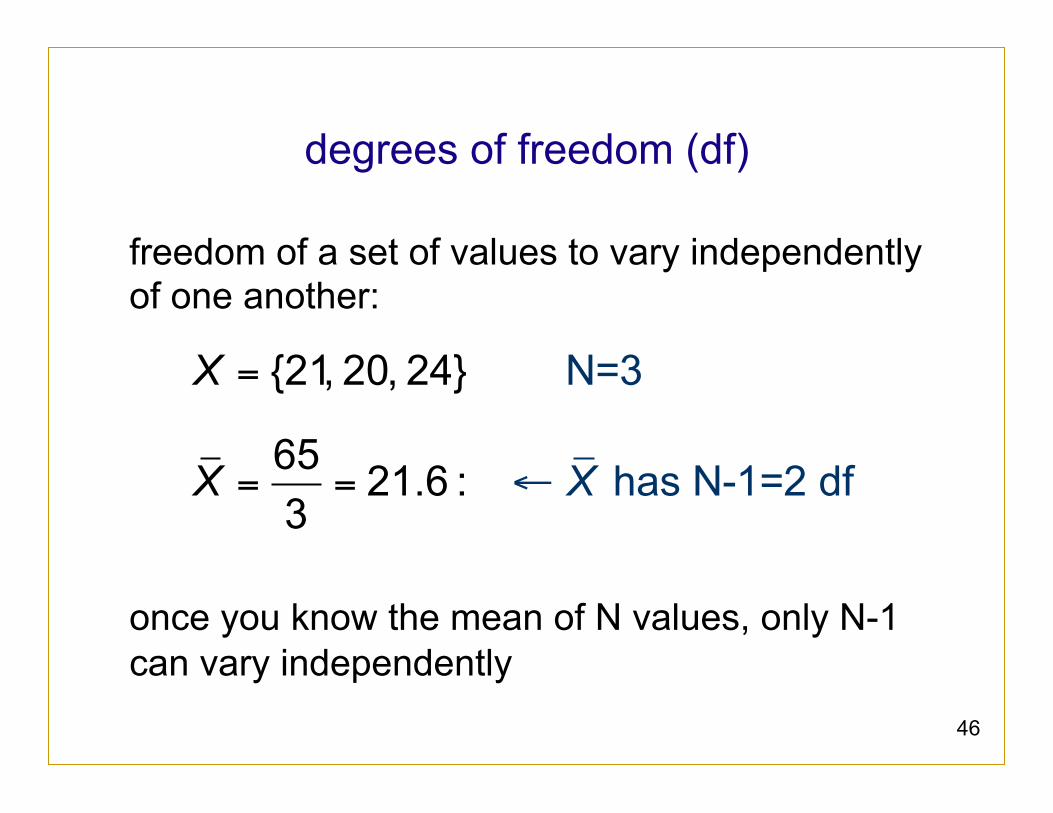
degrees of freedom (df)
freedom of a set of values to vary independently of one another: once you know the mean of N values, only N-1 can vary independently
=
= = ←
{21, 20, 24}
65 2
N=3
has1. N6 : -1=3
2 df
X
X X
47
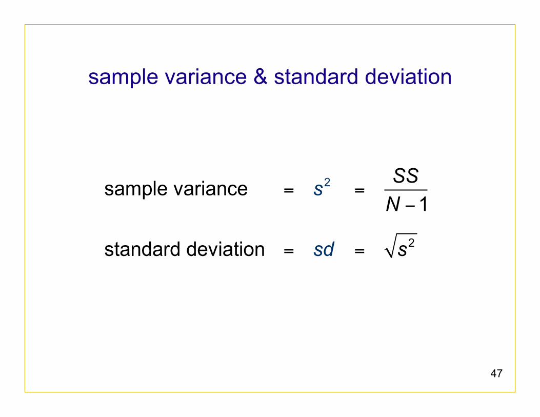
sample variance & standard deviation
= =−
= =
2
2
sample variance1
standard deviation
SS
sd
N
s
s
48
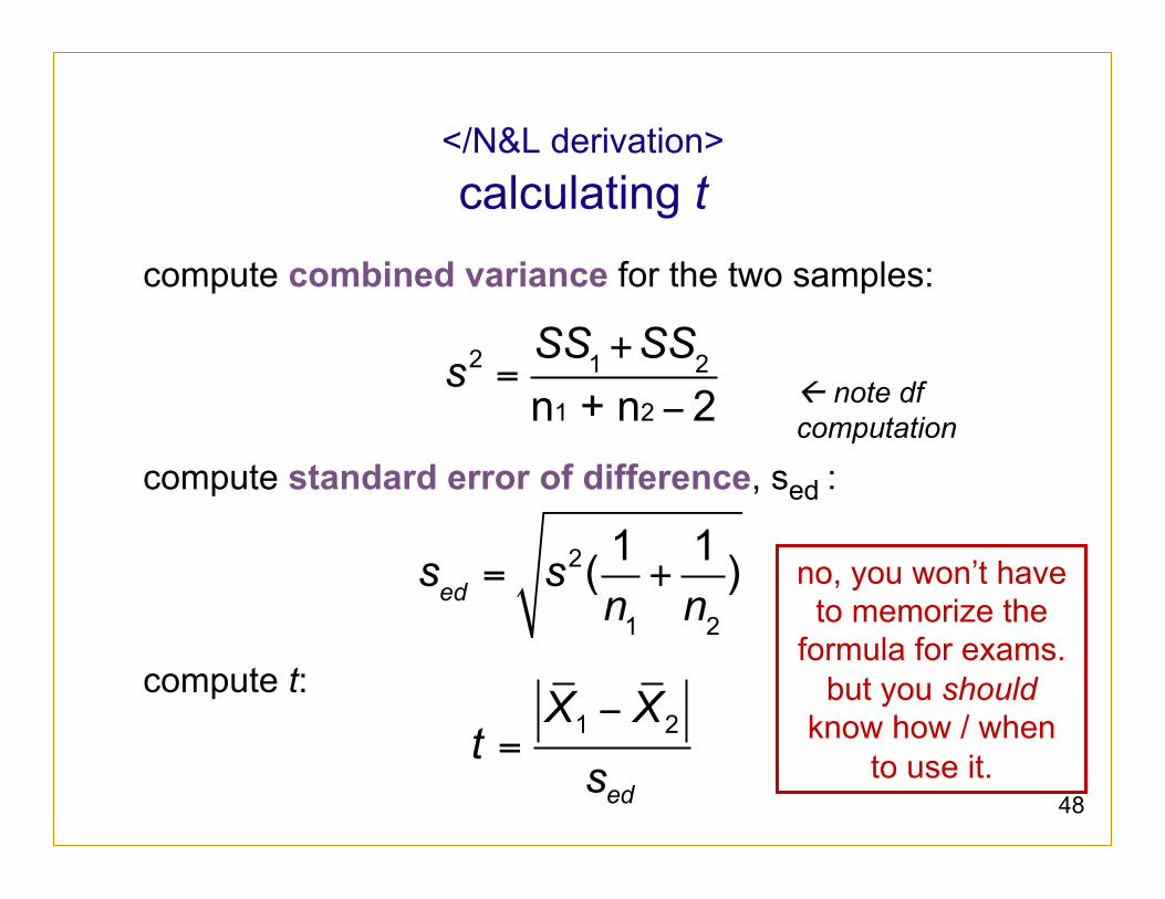
</N&L derivation> calculating t
compute combined variance for the two samples: compute standard error of difference, sed : compute t:
s2 =SS1 +SS2
n1 + n2 − 2
sed = s2( 1n1+1n2)
−=
1 2
ed
X Xt
s
ß note df computation
no, you won’t have to memorize the
formula for exams. but you should
know how / when to use it.
49
df .05 .011 12.706 63.6572 4.303 9.9253 3.182 5.8414 2.776 4.6045 2.571 4.032
6 2.447 3.7077 2.365 3.4998 2.306 3.3559 2.262 3.25010 2.228 3.169
11 2.201 3.10612 2.179 3.05513 2.160 3.01214 2.145 2.97715 2.131 2.947
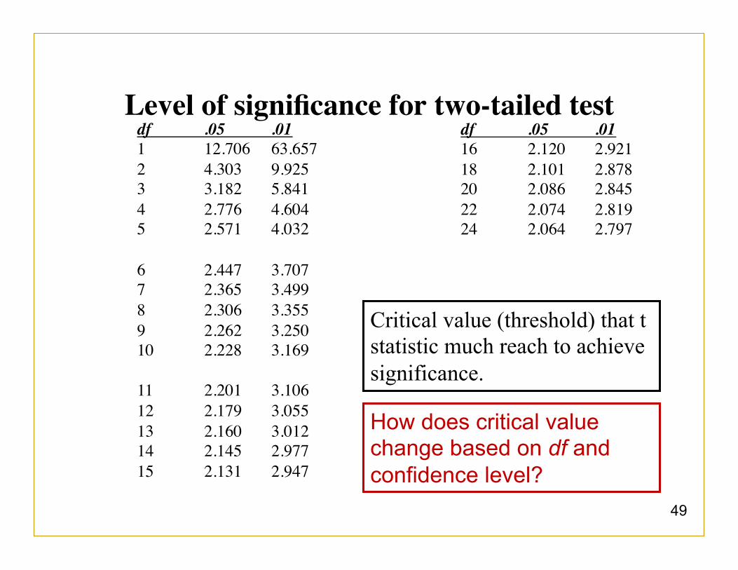
Level of significance for two-tailed testdf .05 .0116 2.120 2.92118 2.101 2.87820 2.086 2.84522 2.074 2.81924 2.064 2.797
Critical value (threshold) that t statistic much reach to achieve significance.
How does critical value change based on df and confidence level?
50
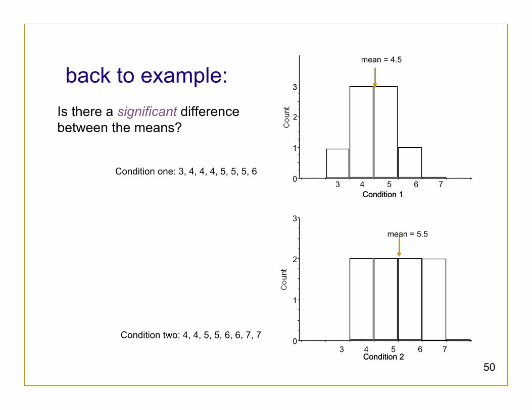
back to example: Is there a significant difference between the means?
Condition one: 3, 4, 4, 4, 5, 5, 5, 6
Condition two: 4, 4, 5, 5, 6, 6, 7, 7
0
1
2
3
Condition 1 Condition 1
0
1
2
3
Condition 2 Condition 2
3 4 5 6 7
mean = 4.5
mean = 5.5
3 4 5 6 7
51
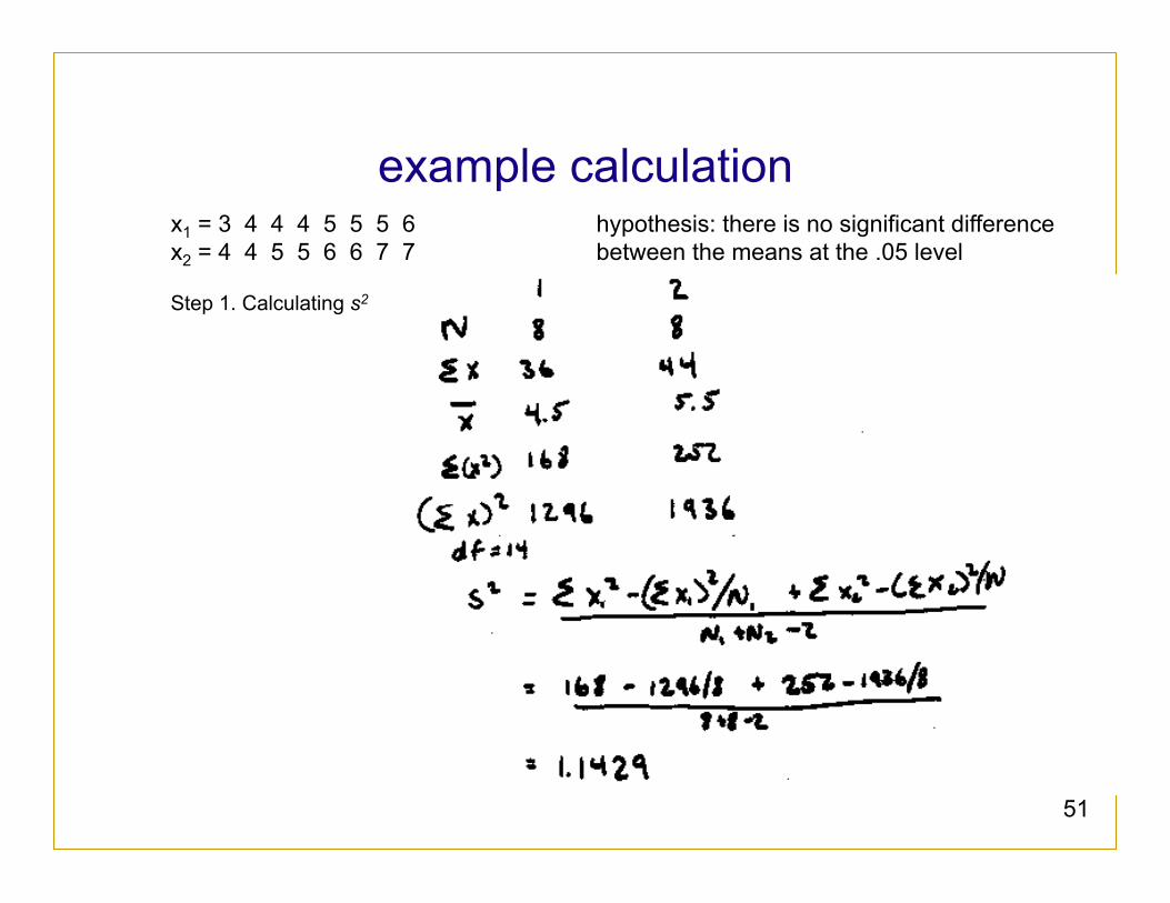
example calculation x1 = 3 4 4 4 5 5 5 6 hypothesis: there is no significant difference x2 = 4 4 5 5 6 6 7 7 between the means at the .05 level Step 1. Calculating s2
52
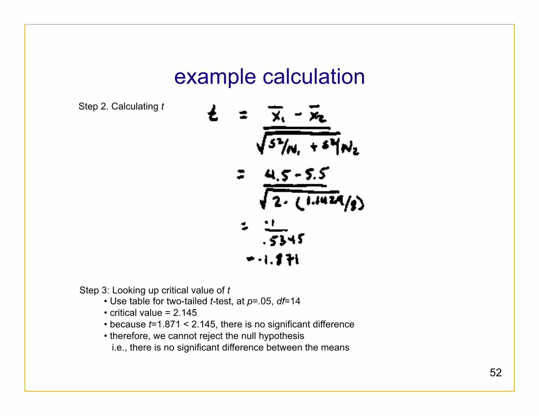
example calculation Step 2. Calculating t
Step 3: Looking up critical value of t • Use table for two-tailed t-test, at p=.05, df=14 • critical value = 2.145 • because t=1.871 < 2.145, there is no significant difference • therefore, we cannot reject the null hypothesis i.e., there is no significant difference between the means
53
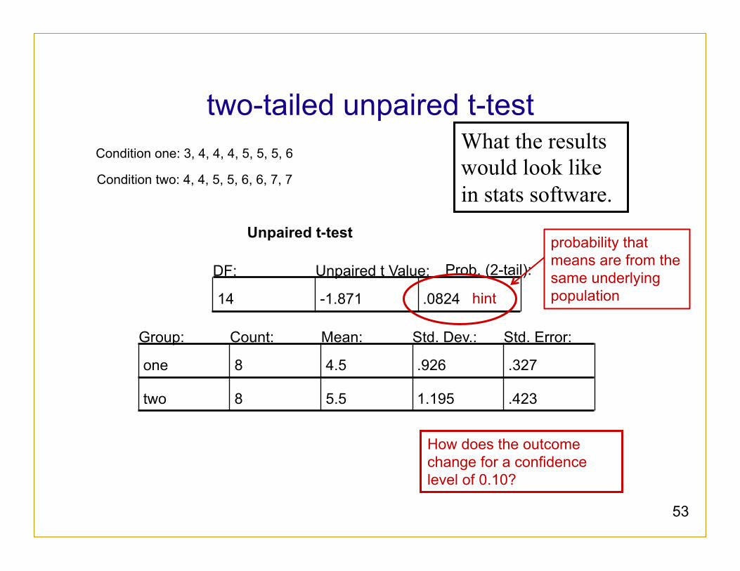
two-tailed unpaired t-test
Unpaired t-test
DF:
14
Unpaired t Value:
-1.871
Prob. (2-tail):
.0824
Group: Count: Mean: Std. Dev.: Std. Error:
one 8 4.5 .926 .327
two 8 5.5 1.195 .423
Condition one: 3, 4, 4, 4, 5, 5, 5, 6
Condition two: 4, 4, 5, 5, 6, 6, 7, 7
What the results would look like in stats software.
How does the outcome change for a confidence level of 0.10?
hint
probability that means are from the same underlying population
54
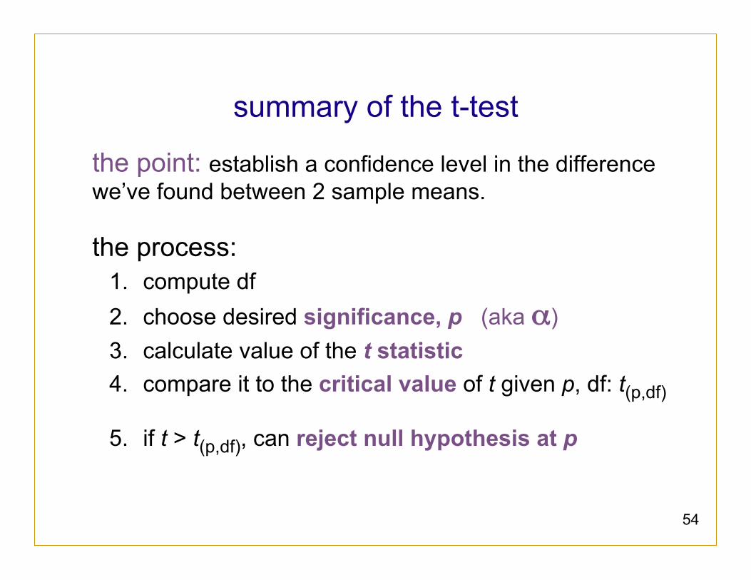
summary of the t-test
the point: establish a confidence level in the difference we’ve found between 2 sample means.
the process: 1. compute df 2. choose desired significance, p (aka α) 3. calculate value of the t statistic 4. compare it to the critical value of t given p, df: t(p,df)
5. if t > t(p,df), can reject null hypothesis at p
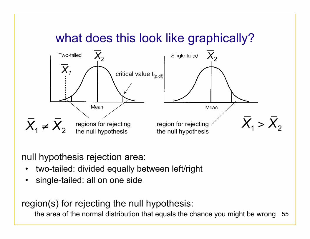
null hypothesis rejection area: • two-tailed: divided equally between left/right • single-tailed: all on one side
region(s) for rejecting the null hypothesis: the area of the normal distribution that equals the chance you might be wrong 55
what does this look like graphically?
≠1 2X X >1 2X Xregions for rejecting the null hypothesis
region for rejecting the null hypothesis
X2 X2
critical value t(p,df) X1
56
you now know
How to answer the following: what is the experimental method? what is an experimental hypothesis? how do I plan an experiment? why are statistics used? within- & between-subject comparisons: how do they differ? how do I compute a t-test? what are the different types of t-tests?
57
additional slides: material I assume you know
types of variables samples & populations normal distribution variance and standard deviation
58
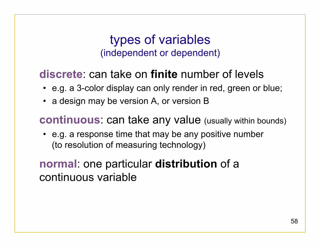
types of variables (independent or dependent)
discrete: can take on finite number of levels • e.g. a 3-color display can only render in red, green or blue; • a design may be version A, or version B
continuous: can take any value (usually within bounds)
• e.g. a response time that may be any positive number (to resolution of measuring technology)
normal: one particular distribution of a continuous variable
59
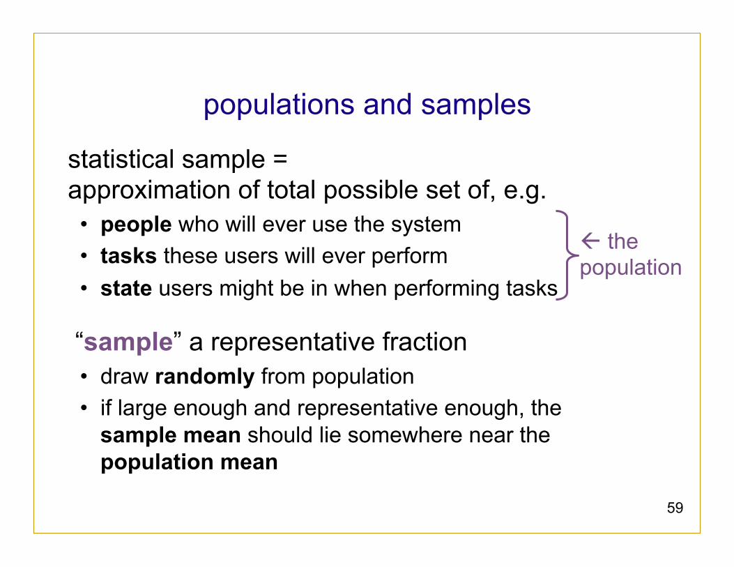
populations and samples
statistical sample = approximation of total possible set of, e.g. • people who will ever use the system • tasks these users will ever perform • state users might be in when performing tasks
“sample” a representative fraction • draw randomly from population • if large enough and representative enough, the
sample mean should lie somewhere near the population mean
ß the population
60
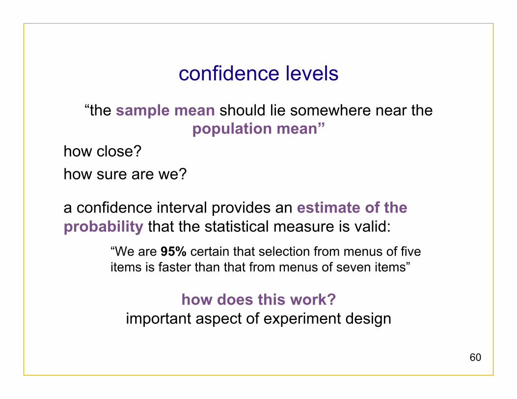
confidence levels
“the sample mean should lie somewhere near the population mean”
how close? how sure are we?
a confidence interval provides an estimate of the probability that the statistical measure is valid:
“We are 95% certain that selection from menus of five items is faster than that from menus of seven items”
how does this work? important aspect of experiment design
61
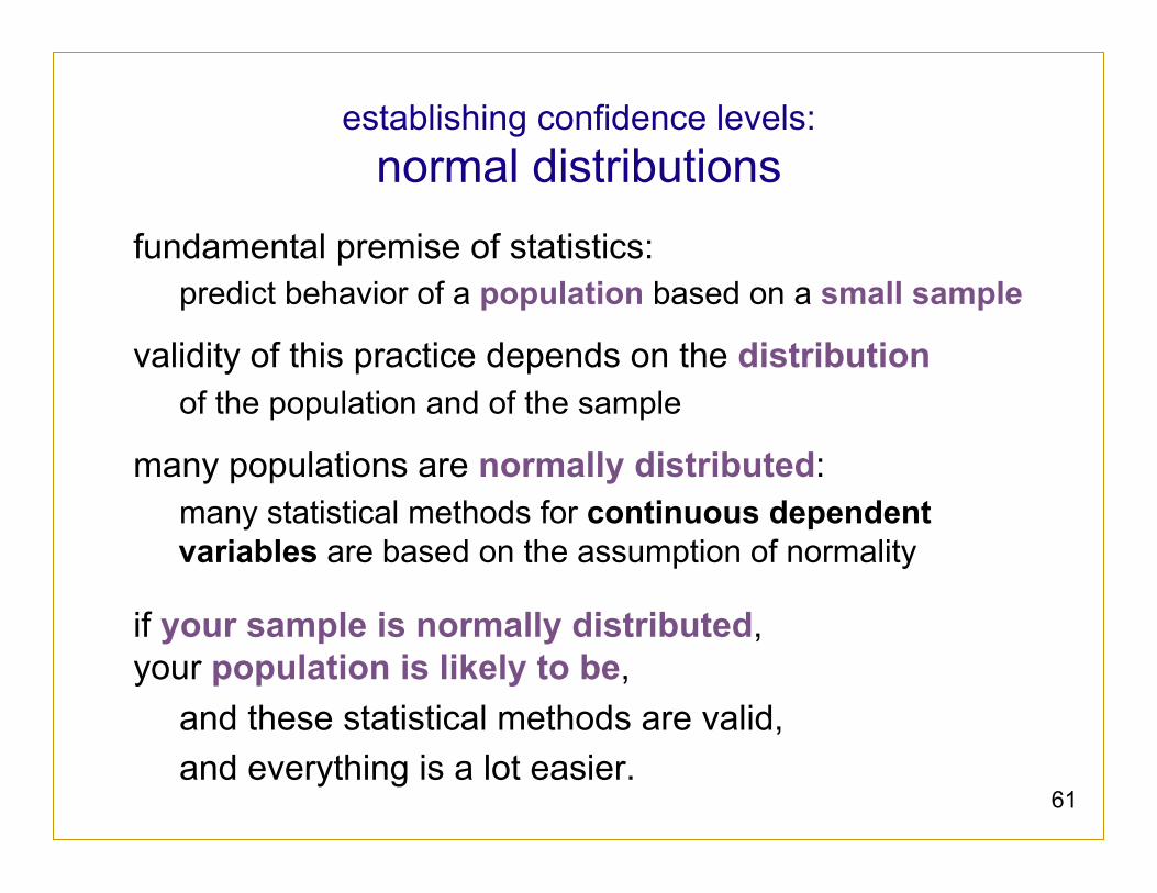
establishing confidence levels: normal distributions
fundamental premise of statistics: predict behavior of a population based on a small sample
validity of this practice depends on the distribution of the population and of the sample
many populations are normally distributed: many statistical methods for continuous dependent variables are based on the assumption of normality
if your sample is normally distributed, your population is likely to be,
and these statistical methods are valid, and everything is a lot easier.
62
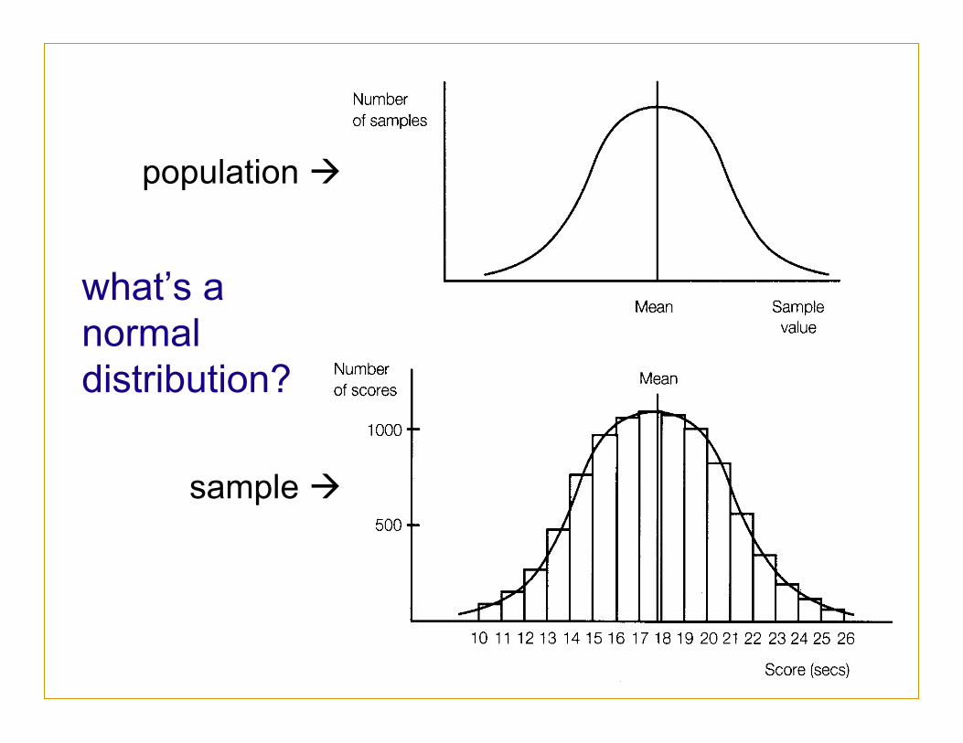
what’s a normal distribution?
population à
sample à
63
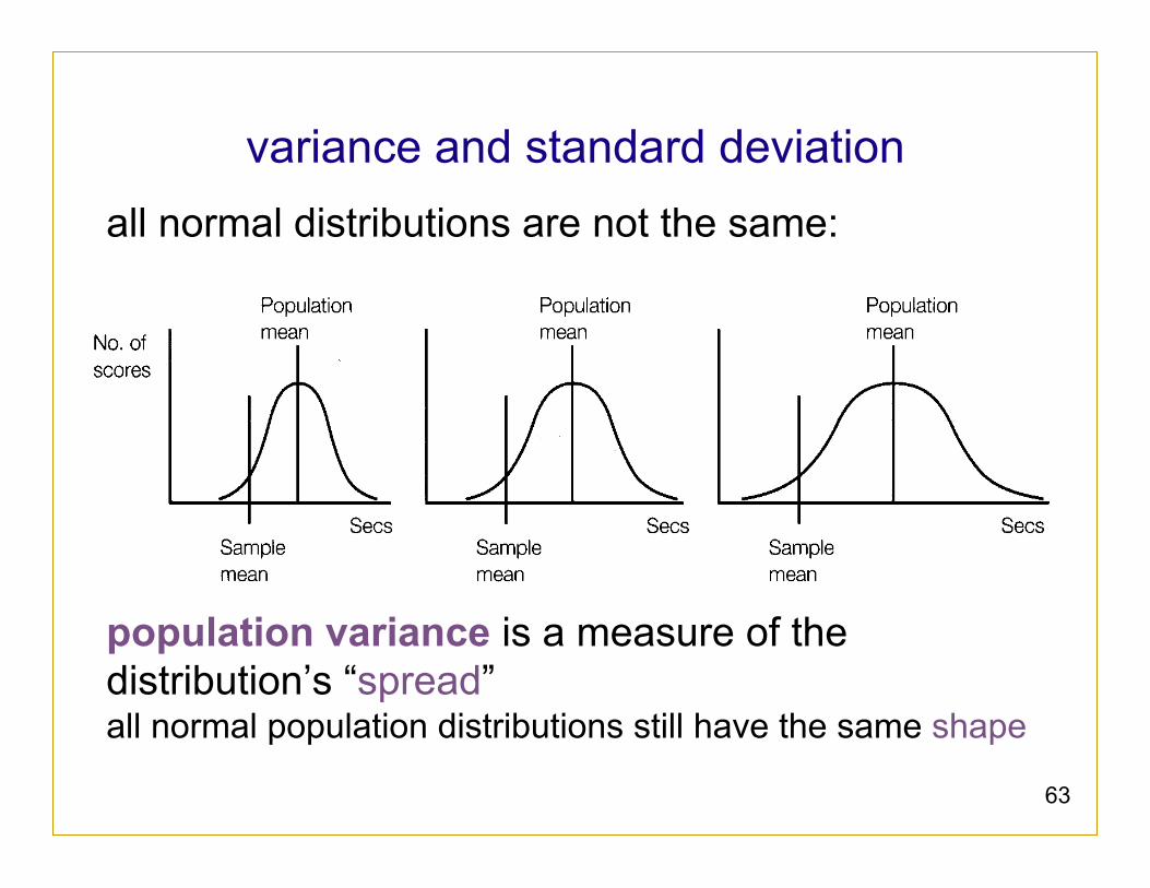
variance and standard deviation all normal distributions are not the same: population variance is a measure of the distribution’s “spread” all normal population distributions still have the same shape
64
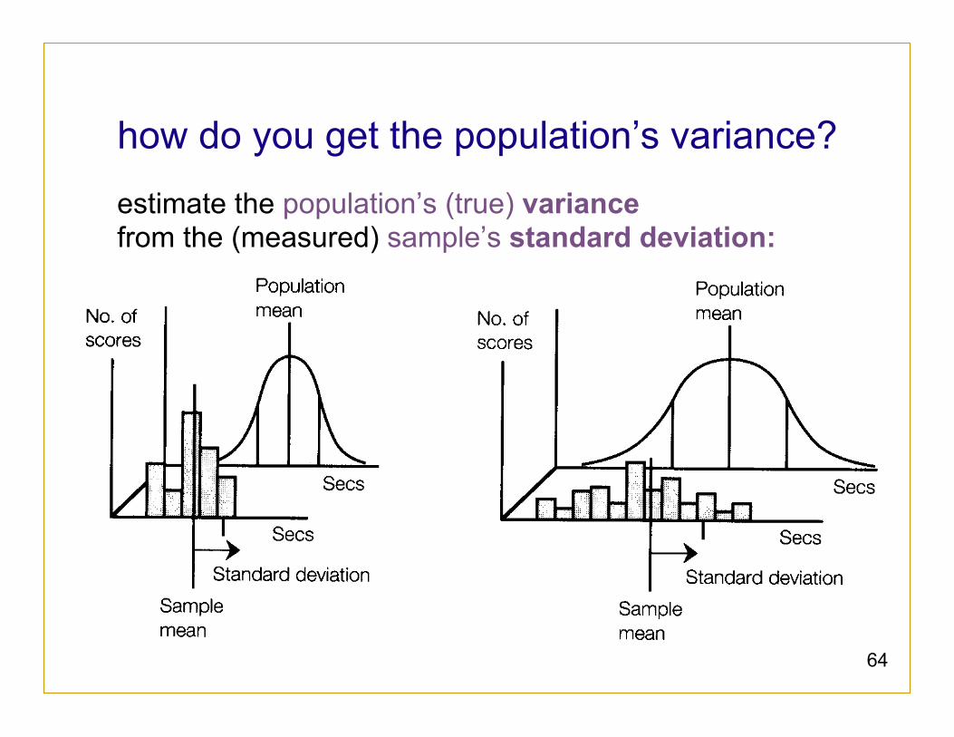
how do you get the population’s variance?
estimate the population’s (true) variance from the (measured) sample’s standard deviation:
65
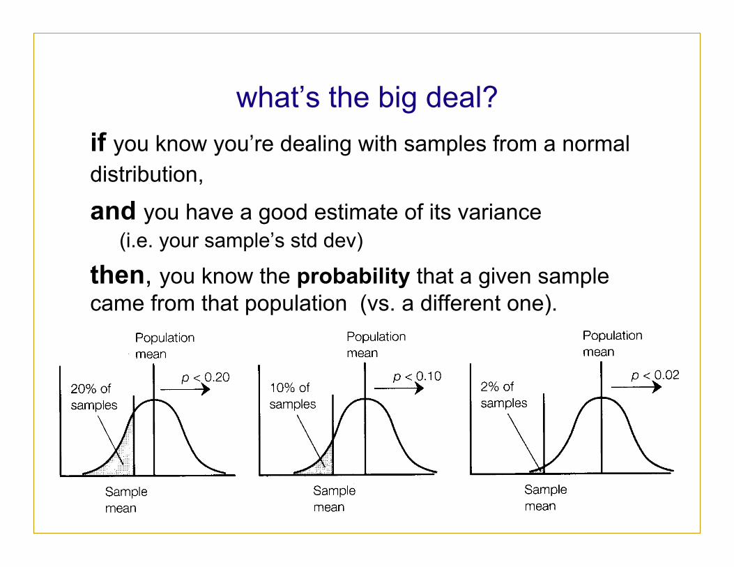
what’s the big deal? if you know you’re dealing with samples from a normal distribution, and you have a good estimate of its variance
(i.e. your sample’s std dev)
then, you know the probability that a given sample came from that population (vs. a different one).


