Photos placed in horizontal position

with even amount of white space

between photos and header

Sandia National Laboratories is a multi-program laboratory managed and operated by Sandia Corporation, a wholly owned subsidiary of Lockheed Martin

Corporation, for the U.S. Department of Energy’s National Nuclear Security Administration under contract DE-AC04-94AL85000. SAND NO. 2011-XXXXP

Unifying the mechanics of continua, cracks, and particles

Stewart Silling Sandia National Laboratories

Albuquerque, New Mexico

MAE Seminar, New Mexico State University, April 11, 2014

SAND2014-2998C

1

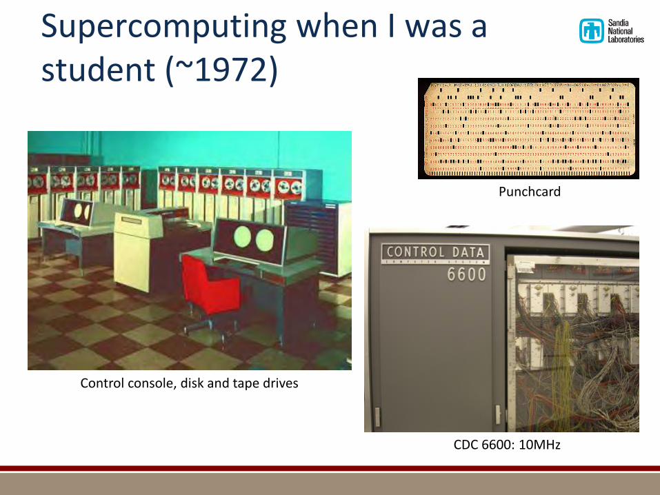
Supercomputing when I was a student (~1972)

CDC 6600: 10MHz

Control console, disk and tape drives

Punchcard

Outline

• Purpose of peridynamics

• Basic equations

• Dynamic fracture examples

• Continuum-particle connection: self-assembly

• Nonlocality in heterogeneous media: composites

• Multiscale peridynamics

3

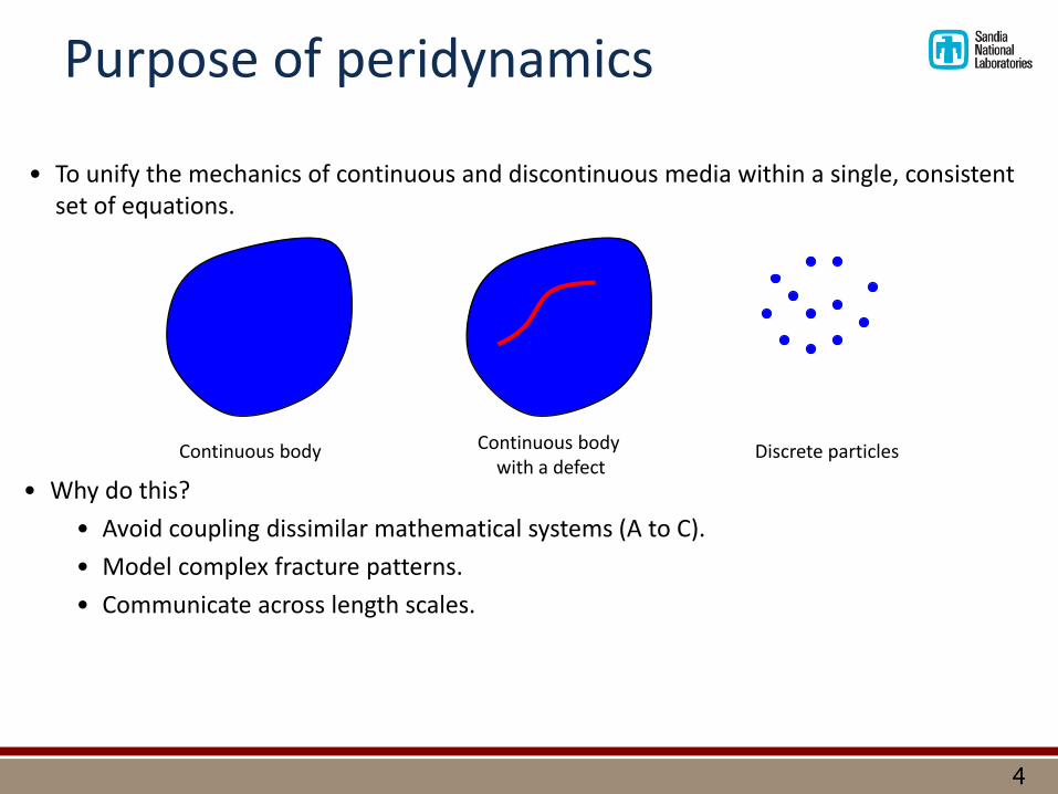
Purpose of peridynamics

• To unify the mechanics of continuous and discontinuous media within a single, consistent set of equations.

Continuous body Continuous body with a defect

Discrete particles

• Why do this?

• Avoid coupling dissimilar mathematical systems (A to C).

• Model complex fracture patterns.

• Communicate across length scales.

4

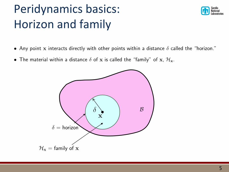
Peridynamics basics: Horizon and family

5

Strain energy at a point

6

Continuum Discrete particles Discrete structures

Deformation

• Key assumption: the strain energy density at 𝐱 is determined by the deformation of its family.

Potential energy minimization yields the peridynamic equilibrium equation

7

Peridynamics basics: Bonds and bond force density

8

Peridynamics basics: The nature of internal forces

𝜎11

𝜎22

𝜎12

𝜌𝑢 𝑥, 𝑡 = 𝛻 ∙ 𝜎 𝑥, 𝑡 + 𝑏 𝑥, 𝑡 𝜌𝑢 𝑥, 𝑡 = 𝑓 𝑞, 𝑥 𝑑𝑉𝑞𝐻𝑥

+ 𝑏 𝑥, 𝑡

Standard theory Stress tensor field

(assumes continuity of forces)

Peridynamics Bond forces between neighboring points

(allowing discontinuity)

Summation over bond forces Differentiation of surface forces

𝑞

𝑓 𝑞, 𝑥

𝜎𝑛

𝑛

𝑥

9

Force state maps bonds onto bond forces Stress tensor maps surface

normal vectors onto surface forces

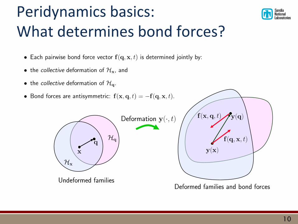
Peridynamics basics: What determines bond forces?

10

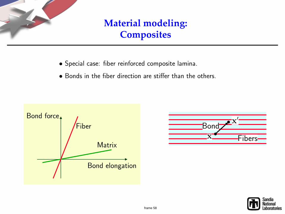
Bond based materials

• If each bond response is independent of the others, the resulting material model is called bond-based.

• The material model is then simply a graph of bond force density vs. bond strain. • Main advantage: simplicity. • Main disadvantage: restricts the material response.

• Poisson ratio always = 1/4.

Bond force density

Bond strain

11

Damage due to bond breakage • Recall: each bond carries a force. • Damage is implemented at the bond level.

• Bonds break irreversibly according to some criterion. • Broken bonds carry no force.

• Examples of criteria: • Critical bond strain (brittle). • Hashin failure criterion (composites). • Gurson (ductile metals).

Bond strain

Bond force density Bond breakage

Critical bond strain damage model

12

Autonomous crack growth

Broken bond

Crack path

• When a bond breaks, its load is shifted to its neighbors, leading to progressive failure.

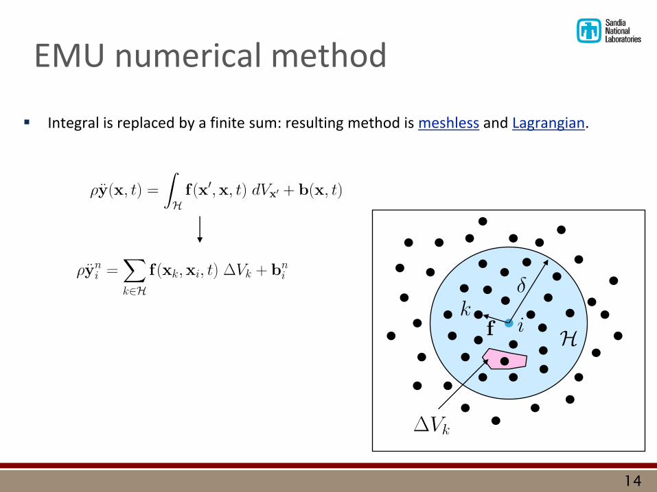
EMU numerical method

14

Integral is replaced by a finite sum: resulting method is meshless and Lagrangian.

Energy balance for a crack: validation

• This confirms that the energy consumed per unit crack growth area equals the expected value from bond breakage properties.

From bond

properties, energy

release rate

should be

G = 0.013

W = External work

E = Strain energy

W-E = Consumed energy

Crack tip position

Energ

y

Slope = 0.013

15

Dynamic fracture in a hard steel plate

16

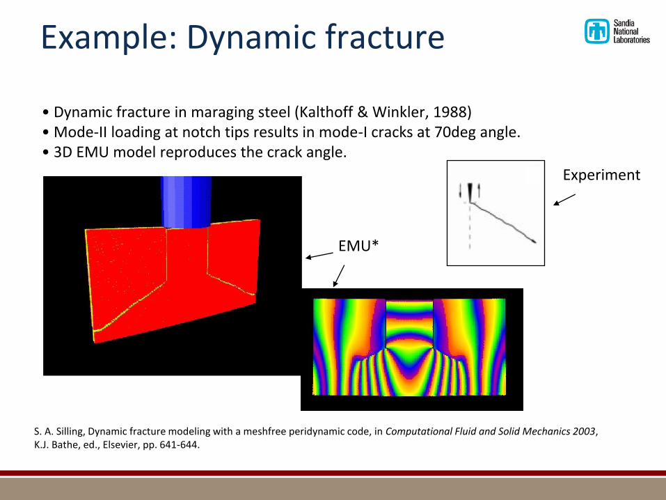
• Dynamic fracture in maraging steel (Kalthoff & Winkler, 1988) • Mode-II loading at notch tips results in mode-I cracks at 70deg angle. • 3D EMU model reproduces the crack angle.

EMU*

Experiment

S. A. Silling, Dynamic fracture modeling with a meshfree peridynamic code, in Computational Fluid and Solid Mechanics 2003, K.J. Bathe, ed., Elsevier, pp. 641-644.

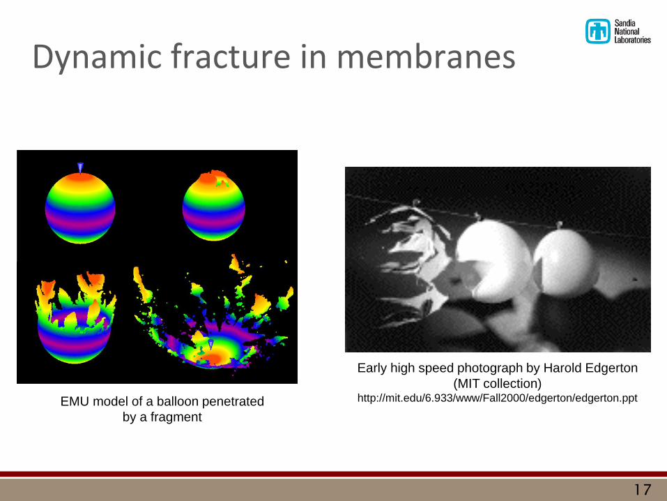
Dynamic fracture in membranes

17

Early high speed photograph by Harold Edgerton

(MIT collection) http://mit.edu/6.933/www/Fall2000/edgerton/edgerton.ppt EMU model of a balloon penetrated

by a fragment

Pressurized shell struck by a fragment

Video

Examples: Membranes and thin films

Oscillatory crack path Crack interaction in a sheet Aging of a film

Videos

19

Dynamic fracture in PMMA: Damage features

Microbranching

Mirror-mist-hackle transition*

* J. Fineberg & M. Marder, Physics Reports 313 (1999) 1-108

EMU crack surfaces EMU damage

Smooth

Initial defect

Microcracks

Surface roughness

20

Dynamic fracture in PMMA: Crack tip velocity

• Crack velocity increases to a critical value, then oscillates.

Time (ms)

Cra

ck tip

ve

locity (

m/s

)

EMU Experiment*

* J. Fineberg & M. Marder, Physics Reports 313 (1999) 1-108

21

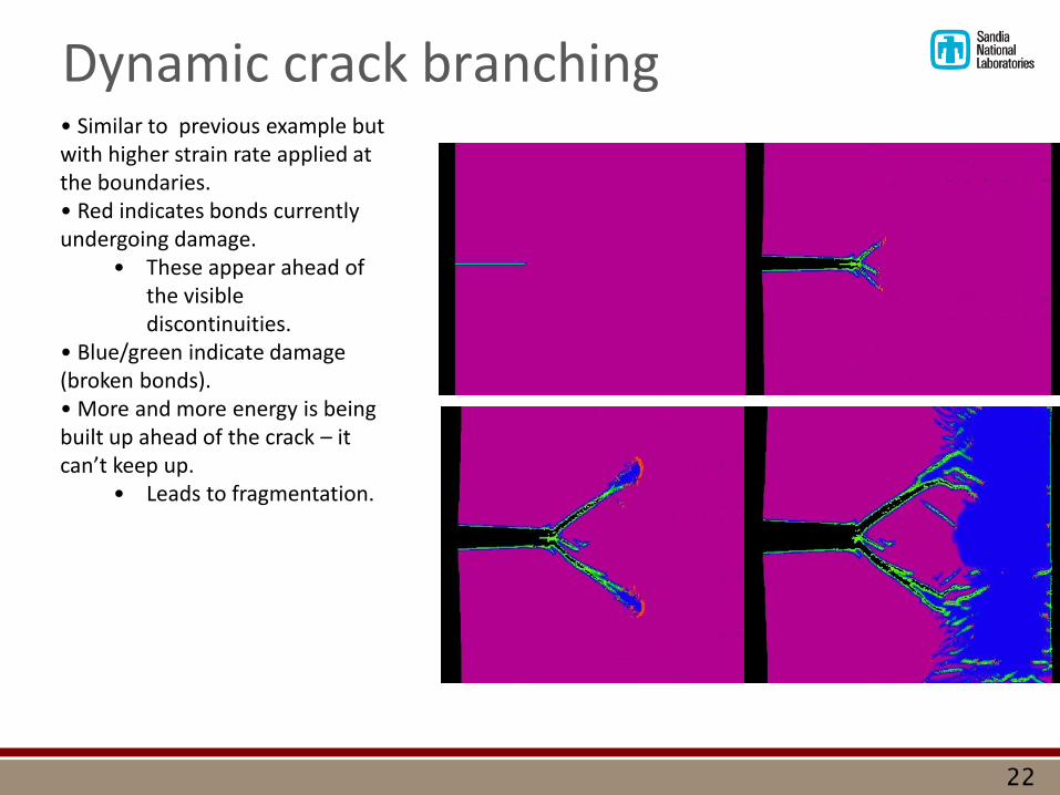
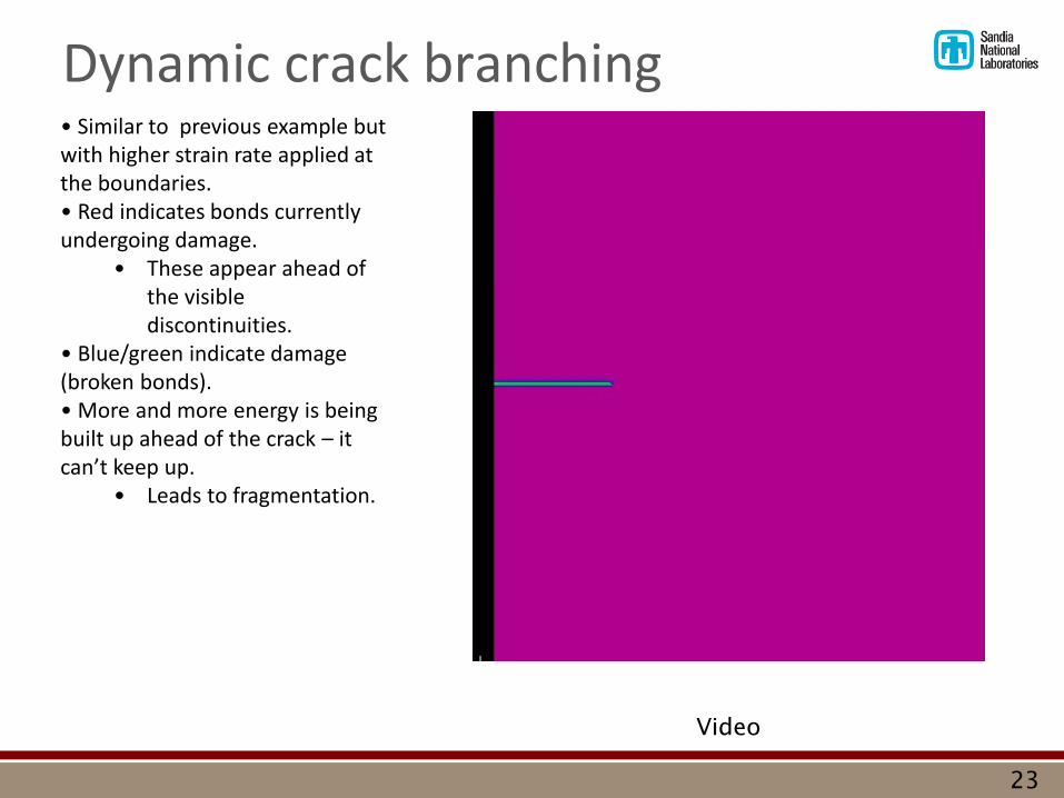
Dynamic crack branching • Similar to previous example but with higher strain rate applied at the boundaries. • Red indicates bonds currently undergoing damage.

• These appear ahead of the visible discontinuities.

• Blue/green indicate damage (broken bonds). • More and more energy is being built up ahead of the crack – it can’t keep up.

• Leads to fragmentation.

22

Dynamic crack branching • Similar to previous example but with higher strain rate applied at the boundaries. • Red indicates bonds currently undergoing damage.

• These appear ahead of the visible discontinuities.

• Blue/green indicate damage (broken bonds). • More and more energy is being built up ahead of the crack – it can’t keep up.

• Leads to fragmentation.

23

Video

Example: Impact on reinforced concrete

Video

Nonlocality – is it real?

25

• It is commonly assumed that the local model (PDE-based) is an excellent approximation for continuous media, due to the small size of interatomic distances.

• This is true if we model the system in sufficient detail. • When we use a “smoothed out” displacement field, nonlocality appears in the

equations. Example…

Compliant

Stiff

Layered composite (1D)

𝑢𝑠 𝑥

𝑢𝑐 𝑥, 𝑦

Nonlocality in a homogenized model

26

• Choose to model the composite as a single mass-weighted average displacement field 𝑢 𝑥 .

𝑢 𝑥

𝑥

𝑢 𝑢

𝑢𝑠𝑡𝑖𝑓𝑓

𝑢𝑐𝑜𝑚𝑝𝑙𝑖𝑎𝑛𝑡

Nonlocality in a homogenized model

27

• After computing the force transfer between the phases, the equation of motion turns out to be

Strain

𝑥

Homogenized strain 𝑢 ′(𝑥)

Stiff strain

Compliant strain

Strain in each phase if the homogenized strain follows a step function

Are composites nonlocal? Peridynamic model is more accurate than the local model for predicting stress

concentration in a laminate.

ℎ𝑠 = ℎ𝑐 =0.4mm, 𝐸𝑠 = 150GPa, 𝜇𝑐 =4GPa.

⇒ 1 𝜆 = 1.41mm.

28

Emu 𝛿=2mm

Data of Toubal, Karama, and Lorrain, Composite Structures 68 (2005) 31-36

EMU: contours of longitudinal stress Horizon = 2mm

Splitting and fracture mode change in composites

29

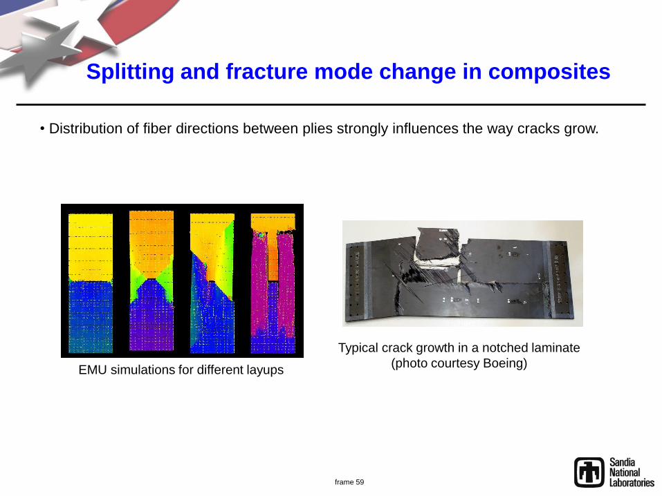
• Distribution of fiber directions between plies strongly influences the way cracks grow.

Typical crack growth in a notched laminate (photo courtesy Boeing)

EMU simulations for different layups

Self-assembly and long-range forces

30

• Potential importance for self-assembled nanostructures. • All forces are treated as long-range.

Nanofiber self-shaping Carbon nanotube

Failure in a nanofiber membrane (F. Bobaru, Univ. of Nebraska)

Dislocation

Self-assembly is driven by long-range forces Image: Brinker, Lu, & Sellinger, Advanced Materials (1999)

Self-assembly example

31

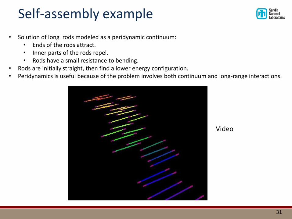
• Solution of long rods modeled as a peridynamic continuum: • Ends of the rods attract. • Inner parts of the rods repel. • Rods have a small resistance to bending.

• Rods are initially straight, then find a lower energy configuration. • Peridynamics is useful because of the problem involves both continuum and long-range interactions.

Video

Self-assembly example

32

Bone: A composite material with many length scales

33

Bone contains a heirarchy of structures at many

length scales. Image: Wang and Gupta, Ann. Rev.

Mat. Sci. 41 (2011) 41-73

Bone structure helps delay, deflect crack growth. Image:

Chan, Chan, and Nicolella, Bone 45 (2009) 427–434

Multiple length scales

Each successive level has a larger length scale (horizon).

Crack process zone

The details of damage evolution are always modeled at level 0.

• Objective: apply a suitable microscale model for processes near a crack tip at whatever length scale is dictated by physics.

• Method: hierarchy of models at different length scales. • Level 0: smallest. • Level > 0: coarsened.

34

Concurrent solution strategy

The equation of motion is applied only within each level.

Higher levels provide boundary conditions (really volume constraints) on lower levels.

Lower levels provide coarsened material properties (including damage) to higher levels.

Level

x

y

Crack

Schematic of communication between levels in a 2D body

2

1

0

35

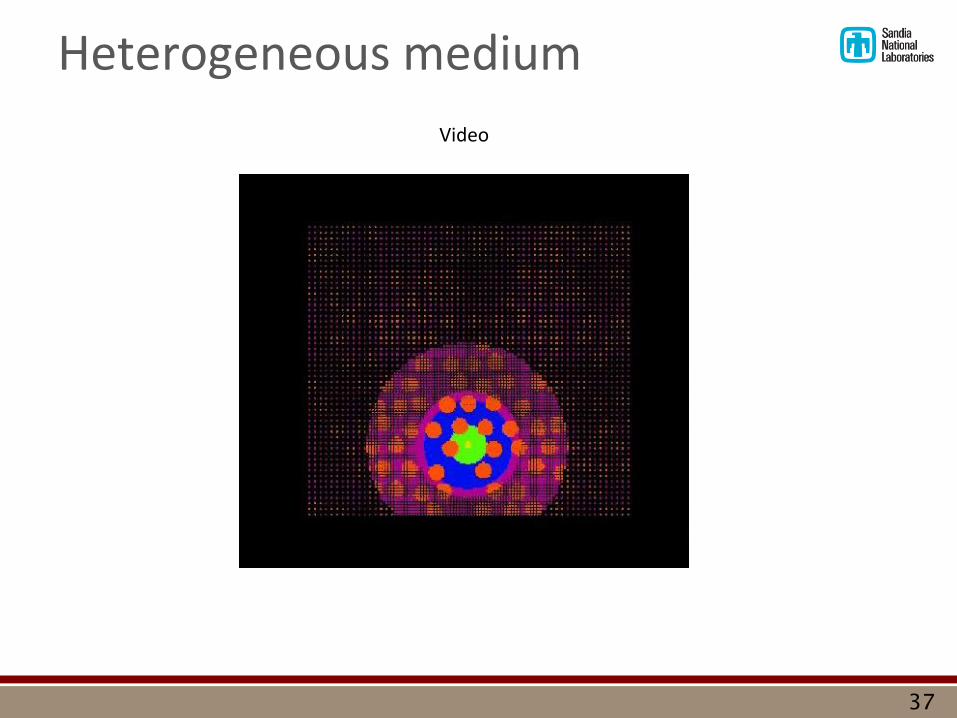
Branching in a heterogeneous medium

• Crack grows between randomly placed hard inclusions.

36

Heterogeneous medium

Video

37

Discussion

38

• All forces are treated as long-range forces. • The basic equations allow discontinuities – compatible with cracks. • Cracks do whatever they want – no need for supplemental equations. • Some practical difficulties:

• Slower than standard finite elements. • Boundary conditions are different than in the standard theory.

frame 39

Extra slides

Critical bond strain: Relation to critical energy release rate

• Can then get the critical strain for bond breakage 𝑠∗ in terms of G.

• Could also use the peridynamic J-integral as a bond breakage criterion.

Crack

Bond strain 𝑠∗

40

Dependencies between levels

Level n problem

Momentum balance

Define boundary conditions

Coarse grain material properties

Deformation Boundary condition

Material properties

Level

41

Flow of information in a time step

= computed deformation

Time step m

Leve

l n

Momentum balance

Define boundary conditions

Coarse grain material properties

42

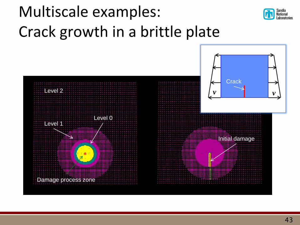
Multiscale examples: Crack growth in a brittle plate

Level 2

Level 1 Level 0

Damage process zone

Initial damage

v v

Crack

43

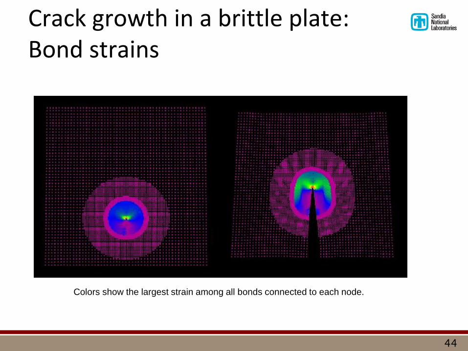
Crack growth in a brittle plate: Bond strains

Colors show the largest strain among all bonds connected to each node.

44

Levels move as the crack grows

Damage process zone

v1 velocity

45

Results with and without multiscale • All three levels give essentially the

same answer. • Higher levels substantially reduce

the computational cost.

0 Levels

1 Level 2 Levels

Bo

un

dar

y lo

ad

Boundary displacement

Level Wall clock time (min) with

28K nodes in coarse grid

Wall clock time (min) with

110K nodes in coarse grid

0 30 168

2 8 16

46

Contact mechanics: Rigid spherical indenter

Level 2 Level 0

Rigid sliding boundary

47

Spherical indenter, ctd.

Hertz cone crack

Radial cracks

Fragmentation pattern

48

Multiscale method discussion

• Advantages • Avoids need for strong coupling (forces acting between different levels). • Combines multiscale with adaptive refinement. • Provides damaged material properties to higher levels.

• Disadvantages

• Difficult to know where to unrefine. • Pervasive fracture leads to a large number of level 0 DOFs. • Don’t yet have a general coarse graining method for heterogenous media.

49

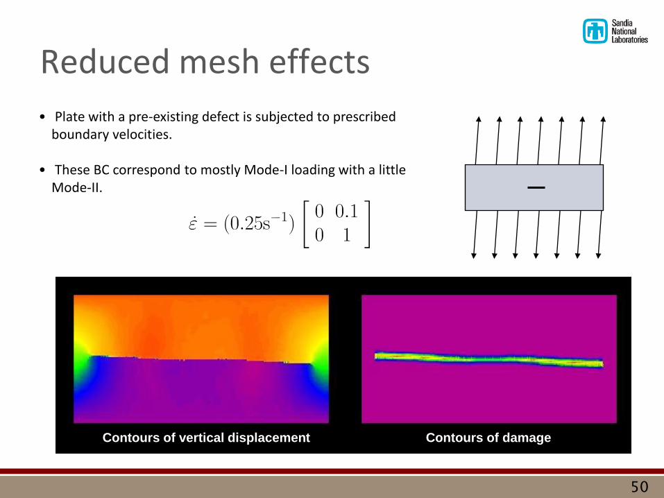
Reduced mesh effects

• Plate with a pre-existing defect is subjected to prescribed boundary velocities.

• These BC correspond to mostly Mode-I loading with a little Mode-II.

Contours of vertical displacement Contours of damage

50

Effect of rotating the grid

Damage Damage, rotated grid

Damage Displacement

Network of identical bonds in many

directions allows cracks to grow in

any direction.

Original grid direction

30deg

Rotated grid direction

51

Convergence in a fragmentation problem

Dx = 3.33 mm

Dx = 2.00 mm

Dx = 1.43 mm

Dx = 1.00 mm

Brittle ring with

initial radial velocity

52

Convergence in a fragmentation problem

Dx (mm) Mean

fragment

mass (g)

3.33 27.1

2.00 37.8

1.43 35.9

1.00 33.5

Cumulative distribution function for 4 grid spacings

1.00mm

1.43mm

2.00mm

3.33mm

Solution appears essentially converged

53

Dynamic fracture

54

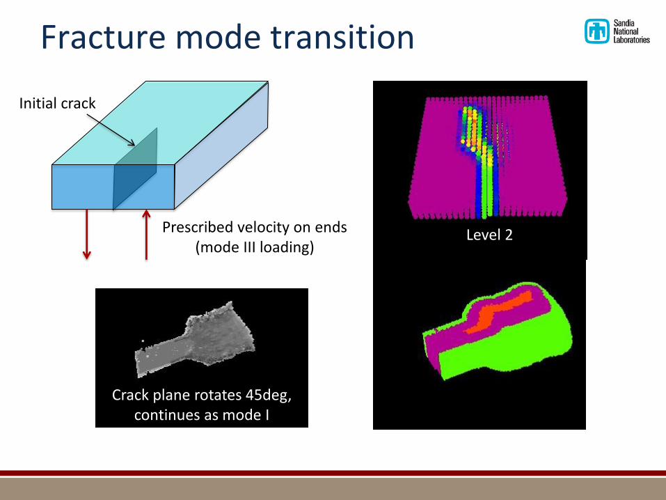
Fracture mode transition

Initial crack

Prescribed velocity on ends (mode III loading)

Level 2

Crack plane rotates 45deg, continues as mode I

frame 56

Nonlocality as a result of homogenization

• Homogenization, neglecting the natural length scales of a system, often doesn’t give good answers.

Indentor Real

Homogenized, local Stress

Claim: Nonlocality is an essential feature of a realistic homogenized model of a heterogeneous material.

frame 57

Proposed experimental method for measuring the peridynamic horizon

• Measure how much a step wave spreads as it goes through a sample.

• Fit the horizon in a 1D peridynamic model to match the observed spread.

Time

Free surface velocity

Peridynamic 1D

Visar

Spread

Projectile Sample

Visar

Laser

Local model would predict zero spread.

frame 58

Material modeling: Composites

frame 59

Splitting and fracture mode change in composites

• Distribution of fiber directions between plies strongly influences the way cracks grow.

Typical crack growth in a notched laminate

(photo courtesy Boeing) EMU simulations for different layups

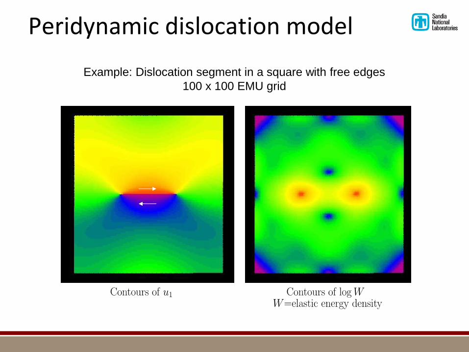
Peridynamic dislocation model

Example: Dislocation segment in a square with free edges

100 x 100 EMU grid

Example of long-range forces: Nanofiber network

Nanofiber membrane (F. Bobaru, Univ. of Nebraska)

Nanofiber interactions due to van der Waals forces

• Peridynamics treats all internal forces as long-range. • This makes it a natural way to treat van der Waals and

surface forces.

Concurrent solution strategy

Crack

Level n

Level 2

Level 1

Level 0:

Within distance d of ongoing damage

Level 0

Level 1

Level 2

Level n

Time R

efin

e

Coa

rsen

Solve (fine)

Solve (coarse)

Refin

e

Coa

rsen

Concurrent solution strategy Level 0 region follows the crack tip

• Refinement:

• Level 1 acts as a boundary condition on level 0.

• Coarsening:

• Level 0 supplies material properties (e.g., damage) to higher levels.

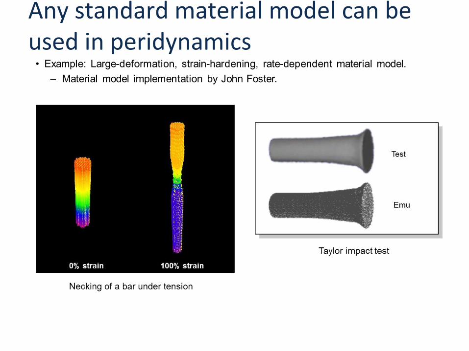
Any standard material model can be used in peridynamics

Rescaling an elastic material model

Comparison with XFEM, interface elements

0

2

4

6

8

10

12

14

16

18

20

22

24

0 0.004 0.008 0.012 0.016 0.02

interface element model (=1/3)XFEM model (=0.22)Pd run 9e5 (=1/3, 3 pt BC)Pd run 9e5 (=1/3, 6 pt BC)

Fy (

N)

DUy (mm)

mesh: ds=0.05 mm, horizon = 6 ds

Peridynamics basics: The nature of internal forces

𝜌𝑢 𝑥, 𝑡 = 𝛻 ∙ 𝜎 𝑥, 𝑡 + 𝑏 𝑥, 𝑡 𝜌𝑢 𝑥, 𝑡 = 𝑓 𝑞, 𝑥 𝑑𝑉𝑞𝐻𝑥

+ 𝑏 𝑥, 𝑡

Standard theory Stress tensor field

(assumes contact forces and smooth deformation)

Peridynamics Bond forces within small neighborhoods

(allow discontinuity)

𝑓 𝑞, 𝑥 𝑥

𝑞

Body

𝜎𝑛

𝑛

Internal surface

Summation over bond forces

Differentiation of contact forces

Family of 𝑥

Horizon 𝛿

Peridynamics basics: States

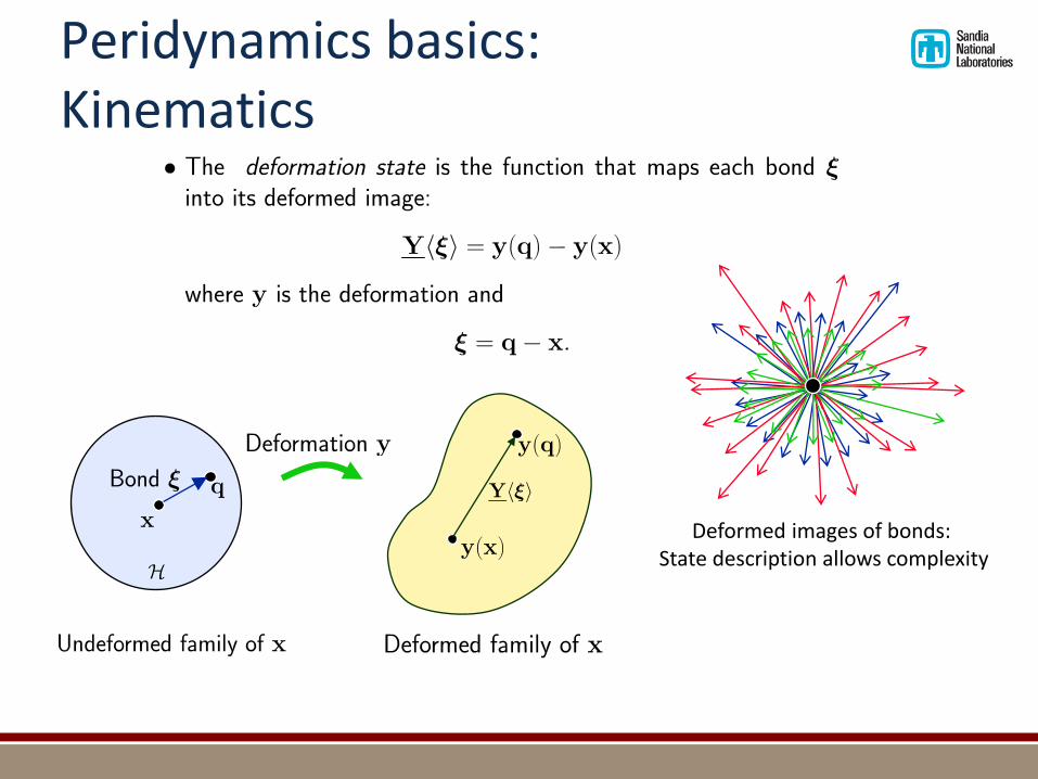
Peridynamics basics: Kinematics

Deformed images of bonds: State description allows complexity

Peridynamics basics: Force state

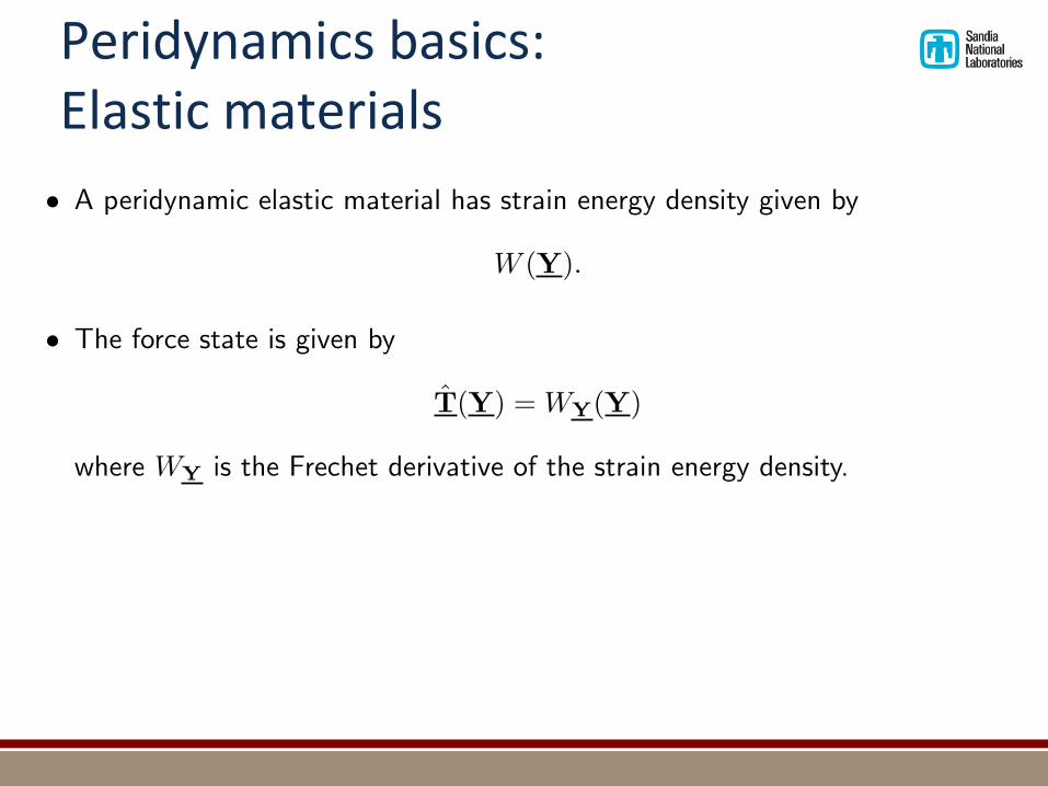
Peridynamics basics: Elastic materials

Peridynamics converges to the local theory

In this sense, the standard theory is a subset of peridynamics.

*Joint work with R. Lehoucq

Some results about peridynamics

• For any choice of horizon, we can fit material model parameters to match the bulk properties and energy release rate.

• Using nonlocality, can obtain material model parameters from wave dispersion curves (Weckner).

• Coupled coarse scale and fine scale evolution equations can be derived for composites (Lipton and Alali).

• A set of discrete particles interacting through any multibody potential can be represented exactly as a peridynamic body.

• Well posedness has been established under certain conditions (Mangesha, Du, Gunzburger, Lehoucq).

EMU numerical method

• Integral is replaced by a finite sum: resulting method is meshless and Lagrangian.

Discretized model in the reference configuration

• Looks a lot like MD.

• Unrelated to Smoothed Particle Hydrodynamics

• SPH solves the local equations by fitting spatial derivatives to the current node values.

Example: Dynamic fracture

• Dynamic fracture in maraging steel (Kalthoff & Winkler, 1988) • Mode-II loading at notch tips results in mode-I cracks at 70deg angle. • 3D EMU model reproduces the crack angle.

EMU*

Experiment

S. A. Silling, Dynamic fracture modeling with a meshfree peridynamic code, in Computational Fluid and Solid Mechanics 2003, K.J. Bathe, ed., Elsevier, pp. 641-644.

Shear loading

Bond strain Damage process zone

Polycrystals: Mesoscale model*

Large favors trans-granular fracture.

*

*

g

i

s

sβ

= 1 = 4 = 0.25

• What is the effect of grain boundaries on the fracture of a polycrystal?

Bond strain

Bond force

*is

*gs

Bond within a grain

Interface bond

* Work by F. Bobaru & students

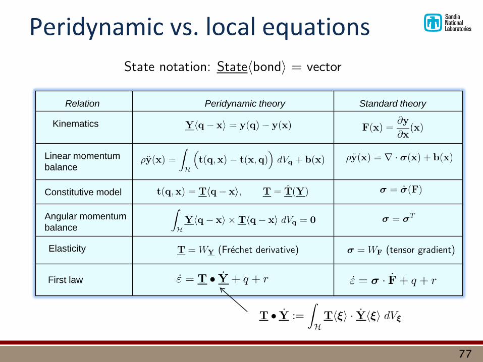
Peridynamic vs. local equations

Kinematics

Constitutive model

Linear momentum

balance

Angular momentum

balance

Peridynamic theory Standard theory Relation

Elasticity

First law

77

frame 78

Discrete particles and PD states

frame 79

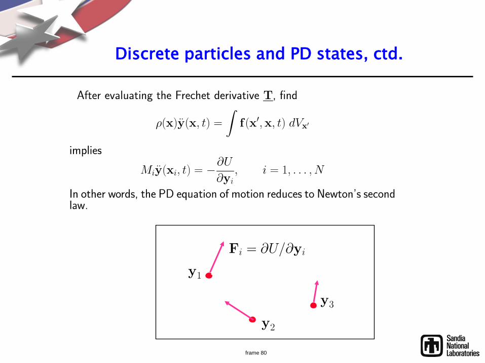
Discrete particles and PD states, ctd.

frame 80

Discrete particles and PD states, ctd.

Why this is important

• The standard PDEs are incompatible with the essential physical nature of cracks.

• Can’t apply PDEs on a discontinuity.

• Typical FE approaches implement a fracture model after numerical discretization.

• Need supplemental kinetic relations that are understood only in idealized cases.

?

Real crack FE

Complex crack path in a composite

81