Credit Rationing in DevelopingCountries : An Overview of the

Theory

Parikshit Ghosh, Dilip Mookherjee, Debraj Ray

February 24, 2013

Introduction to Credit Market

• Demand for Credit -

1. Fixed Capital - Capital required for a new start up or

expansion of existing production lines.

2. Working Capital - Capital Required for ongoing production

activity.

3. Consumption Credit - Demanded by poor individuals who

have suffered an income shock.

• Supply of Credit

1. Institutional Lenders - Commercial or cooperative banks.

2. Informal Sector - Village money lenders.

• In an ideal world of perfect competition, the demand for

credit would have been supplied by the institutional lenders at

the going interest rate. The informal sector would not have

existed.

• Why does credit market fail -

1. Informational Problems - Lack of information regarding

the characteristics of the borrower, difficulty of monitoring

what is done with the loan (which may give rise to the

problem of involuntary default).

2. Strategic Default - Contract enforcement problems (due

to weak legal institutions). Particularly applicable for

developing countries.

1

Credit Market

• Rural Credit Market

1. Institutional Lenders :

(a) The problem is such lenders do not have much knowledge

about characteristics or activities of their clientele.

(b) In presence of uncertainty about project returns and

limited liability there would be too much risk taken by

the borrowers which the bank dose not want.

Even without limited liability, the borrowers who would

be able to pay under all contingencies would be the rich

(higher collateral). Thus there is discrimination against

poor borrowers who turn to the informal sector for loans.

2. Informal Lenders :

(a) Better information regarding characteristics and

activities of clientele.

(b) Collateral unacceptable to banks (working to pay off

loan) may be acceptable to informal lenders.

2

Credit Market

• Features of Informal Credit Market :

1. Loans are often advanced on the basis of oral agreements,

with little or no collateral, making default a seemingly

attractive option.

2. The credit market is usually highly segmented, marked by

long term exclusive relationship and repeat lending.

3. Interest rates are much higher on average than bank interest

rates.

4. Significant credit rationing, whereby borrowers are unable

to borrow all they want, or some loan applicants are unable

to borrow at all.

5. Inter linkage of markets.

• The common theme of the different theories which try to

explain these features is that the world of informal credit is

one of missing markets, asymmetric information and incentive

problems.

• This study focuses on two different aspects of the above

mentioned literature -

1. Moral hazard and limited liability, which give rise to the

possibility of involuntary default.

2. Contract enforcement problem, which give rise to the

possibility of strategic (voluntary) default.

3

Moral Hazard and Limited Liability

• Moral Hazard and Limited Liability

– Indivisible projects requires funds of amount L to be viable

– Output is binary; either Q or 0

– Probability of getting Q is p(e), where e is the effort level

of the agent. Assume p′(.) > 0 and p′′(.) < 0.

– Effort cost is e.

– Agents are risk neutral

• The Benchmark (First Best)

– Self Financed Farmer - The optimal effort choice problem

of the self financed farmer is to (if investment takes place

at all)

maxe

[p(e)Q− e− L] (1)

The optimal choice e∗ solves the F.O.C. -

p′(e∗) =

1

Q(2)

e∗ is the efficient first best level of effort. Subsequent

results will be compared against this benchmark.

4

Debt Financed Farmer

• Total debt is R = (1 + i)L, where i is the interest rate.

• Effort choice e is not verifiable by a third party, hence not

contractible (leads to moral hazard).

• There is limited liability : the borrower faces no obligation in

case of outcome failure beyond the amount of wealth he has

put up as collateral (w, assumption - w < L).

• The effort choice problem of a borrower facing a total debt R

is -

maxe

[p(e)(Q− R) + [1− p(e)](−w)− e] (3)

The optimal choice e(R,w) solves the F.O.C. -

p′(e(R,w)) =

1

Q+ w − R(4)

• R ↑⇒ e(R,w) ↓As R goes up, RHS of (4) goes up. Therefore p′(e(R,w))

goes up, which means (p′′(.) < 0) e(R,w) goes down.

Higher debt burden R reduces the borrower’s payoff in the

good state, but not in the bad state (in which case he always

loses w). Thus dampening the incentive to apply effort.

5

Debt Financed Farmer (Continued)

• w ↑⇒ e(R,w) ↑As w goes up, RHS of (4) goes down. Therefore p′(e(R,w))

goes down, which means (p′′(.) < 0) e(R,w) goes up. In

this case nothing changes when the state is good, but when

the state is bad, the borrower has much more to lose. Thereby

prompting more effort so that the good state is realised with

a higher probability.

• Lender’s Profit Function -

π = p(e)R + [1− p(e)]w − L (5)

We can assume that π ≥ 0, because, lender’s can always

choose not to lend. π = 0 is the case of perfect competition.

• π ≥ 0⇒ R > w -

π ≥ 0

⇒ p(e)R + [1− p(e)]w − L ≥ 0

⇒ p(e)[R− w] ≥ L− w > 0

⇒ R > w

(6)

6

Debt Financed Farmer (Continued)

• As R > w, comparing equations (2) and (4), we see that

p′(e∗) < p′(e(R,w)). From concavity of p(.), we conclude

that e∗ > e(R,w). This brings us to our first proposition.

• Proposition 1 - As long as the borrower does not have

enough wealth to guarantee the full value of the loan, the

effort choice will be less than first best.

• This called the debt overhang problem - An indebted farmer

will always put less effort on a debt financed than a self

financed project. This is because he has more to gain in the

good state and also more to lose in the bad state in a self

financed project.

7

Equilibrium Determination of Debt (R)and Effort Choice (e)

• We will fix the lender’s profit at a given level (π). Then we will

look at combinations of e and R which solves the incentive

constraint given by equation (4) and the lender’s profit given

by equation (5).

• Pareto Efficient Equilibrium - One of the solutions above (if

there are more than one) will solve the borrower’s utility

maximisation problem.

• Let us take a look at equations (4) and (5). First equation (4).

It is the incentive constraint of the borrower. The slope of it

in e − R space is p′′(e)(p′(e))2 , which is negative. Now equation

(5), which is the lender’s profit function, will be fixed at some

level. The slope of the iso profit curve in the e − R space is

given by −p′(e)[R−w]p(e) , which is also negative.

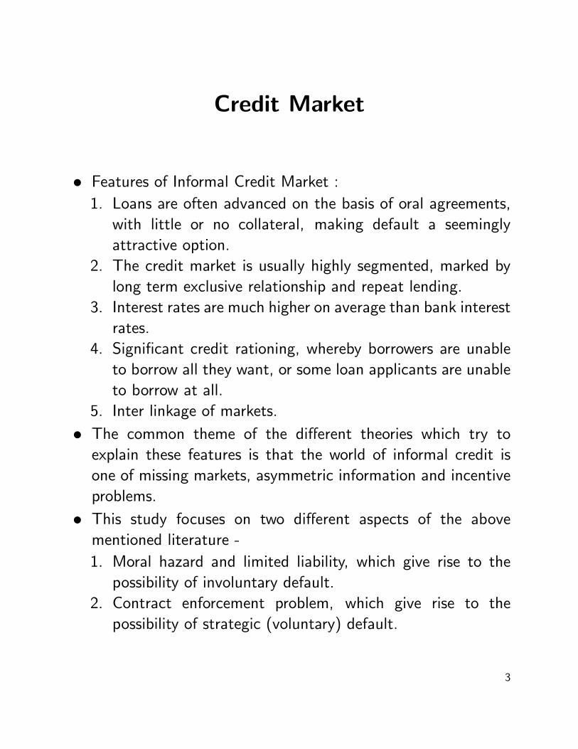
• Consider Figure 1 in the next page

8

Equilibrium Determination of Debt (R)and Effort Choice (e) (Continued)

Figure 1:

• Firstly, as we move down the incentive curve, the borrower’s

payoff increases. Lower debt R increases borrower’s payoff

for any given choice of effort, hence also after adjusting for

optimal choice. So if there are multiple intersections, the one

associated with lowest R is compatible with Pareto efficiency

(when π is kept fixed at the given level).

• Secondly, at the optimum, the incentive curve should be

steeper than the iso profit line. Otherwise a small decrease in

R will increase both lender’s profit and borrower’s utility.

• Thus e in Figure 1 represents the equilibrium.

9

Comparative Statics : Increasing Profitof Lender

Figure 2:

• If we increase lender’s profit, the iso profit curve shifts outwards

as in Figure 2, and in the new Pareto efficient equilibrium, R

is higher, i is higher and e is lower. This brings us to our

second proposition.

• Proposition 2 - (Pareto efficient) equilibria in which lenders

obtain higher profits involve higher debt and interest rates,

but lower levels of effort. Hence this equilibria produce lower

social surplus.

10

Few Observations

• Why dose higher rent extraction (higher π) reduce social

surplus ?

– Higher i is a pure transfer between lender and borrower,

but the greater associated debt burden reduces effort, thus

p(e) increasing chance of failure thus creating a dead-

weight loss.

• Two Extreme Cases -

– Perfect Competition (No Rent Extraction) -

∗ π = 0

∗ By Proposition 2, effort choice would be highest in this

case. But even then, it would be less than first best. So

the problem in choice of effort dose not have much to

do with monopolistic power (even though it aggravates

the problem) but with incentive distortions created by

limited liability.

– Monopoly (Maximum Rent Extraction) -

∗ Iso profit line will be pushed up to the point where it is

tangent to the incentive curve. Let the corresponding

level of R be R. R fixes the interest rate at some i

which provides a ceiling on the interest rate. Even in

more competitive condition ceiling will apply. At this i

if there is excess demand for credit interest rate will not

11

rise to clear the market. We have macro credit rationing.

• We observed that the borrower friendly equilibrium generate

more social surplus. This has implications for social policies.

Policies which reduces interest rate or improve bargaining

power of a borrower will increase effort and productivity.

• However such policy intervention cannot result in improvement

in Pareto efficiency since equilibrium contracts are by definition

are constrained Pareto efficient.

• Can this model generate micro-rationing? Answer is generally

yes.

12

Role of collateral

• Proposition 3: An increase in the size of collateral, w,

leads to a fall in the equilibrium interest rate and debt,

and an increase in the effort level. For a fixed π, the

borrower’s expected income increases; hence, the utility

possibility frontier shift outwards.

• Larger collateral increases the incentive to put in more effort.

Borrower has more to lose in case of failure. If lender’s profit is

held constant then the interest rate should fall because given

higher effort there is now lower default. There is less debt

overhang further increasing incentive is to put in effort.

• Higher effort means higher total surplus. But as lenders’

profits are held fixed the borrowers must get more.

Figure 3:

13

• These result illustrate how interest rate dispersion may arise

even within competitive markets. Amount of collateral affects

the interest rate one has to pay. Rich borrowers are less risky

in two counts -

1. Better collateral in case of default.

2. Because of higher collateral, greater incentives on effort.

Hence less default risk

Hence rich borrowers have access to cheaper credits.

• The second issue of interest is that the way the credit market

functions may aggravate existing inequalities. In some sense,

the poor people are doubly cursed. Neither can they liquidate

their assets to enhance their consumption (because they have

very less assets), nor can they enhance their consumption by

taking credit (because they cannot credibly commit to refrain

from morally hazardous behaviour as effectively as the rich).

14

Repeated Borrowing and Enforcement

In the previous class, we saw how moral hazard problem,

coupled with limited liability gave rise to scenarios where

involuntary default on the part of the borrowers could be

a possibility. Now we focus on the problem of Contract

Enforcement. Here the principal problem faced by the lender

is how to prevent wilful default (i.e. voluntary default) ex-post by

borrowers, who do in fact possess the means to repay their loans.

Assume that the usual enforcement mechanism, i.e., courts,

collateral etc. are absent. Then compliance must be met

through the threat of losing access to credit in the future. Here

a simple infinite horizon repeated lending borrowing game is

used to illustrate such a mechanism, and derive its implications

for rationing and efficiency in credit market. Since involuntary

default is not the focus of this section, so any source of production

uncertainty has been removed.

15

The Model

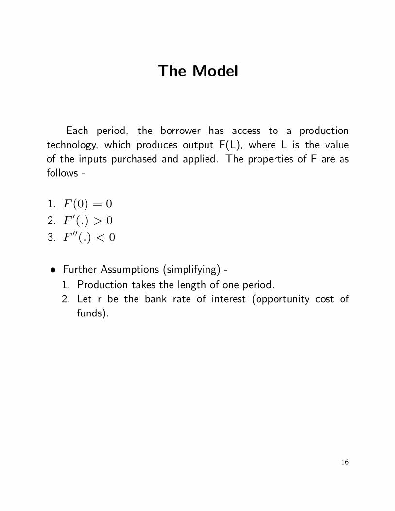
Each period, the borrower has access to a production

technology, which produces output F(L), where L is the value

of the inputs purchased and applied. The properties of F are as

follows -

1. F (0) = 0

2. F ′(.) > 0

3. F ′′(.) < 0

• Further Assumptions (simplifying) -

1. Production takes the length of one period.

2. Let r be the bank rate of interest (opportunity cost of

funds).

16

Benchmark

Now, consider the case of a self financed farmer. His problem

is -

maxL

[F (L)− (1 + r)L] (7)

The F.O.C. is -

F′(L∗) = 1 + r (8)

Where L∗ is the optimal choice of fund that a self financed

farmer wants in this model.

17

Single Lender, Single Borrower - PartialEquilibrium

Now consider the case of a debt-financed farmer.

• Assumptions :

1. Borrower does not accumulate any saving.

2. Borrower lives for an infinite number of periods.

3. Future discount rate δ.

• The Game :

1. Lender can offer a loan contract (L,R = (1 + i)L) or

he can choose not to offer any loan.

2. If the lender offers a contract (L, R), then the borrower

can choose either to comply and repay the lender R, or he

can choose to default and do not repay the lender. If the

lender offers no contract, then the borrower has an outside

option that yields a payoff v.

3. This game is repeated infinite times.

18

For the time t = 0, the extensive form representation of the

game is given below -

We restrict our attention to the class of stationary SPNE,

where the lender offers (L,R) in every period, and follows the

trigger strategy of never offering a loan if the borrower has

defaulted in the immediate past.

19

Pareto Efficient Stationary SPNE

Now the goal is to characterise the Pareto set of all such

stationary SPNE. Consider any period t.

• Long run payoff of the borrower -

– If he defaults in that period -

F (L) +δv

1− δ(9)

– If he complies from then on -

F (L)− R1− δ

(10)

20

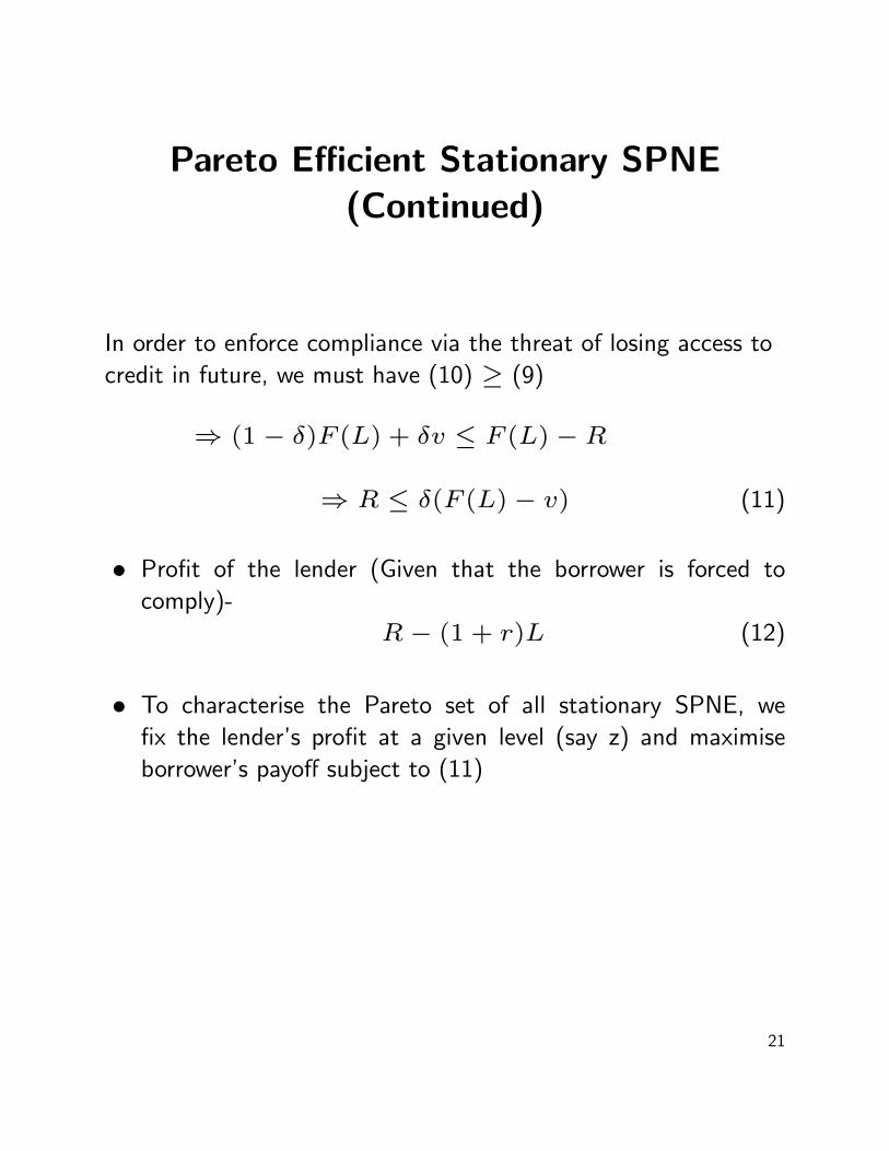
Pareto Efficient Stationary SPNE(Continued)

In order to enforce compliance via the threat of losing access to

credit in future, we must have (10) ≥ (9)

⇒ (1− δ)F (L) + δv ≤ F (L)− R

⇒ R ≤ δ(F (L)− v) (11)

• Profit of the lender (Given that the borrower is forced to

comply)-

R− (1 + r)L (12)

• To characterise the Pareto set of all stationary SPNE, we

fix the lender’s profit at a given level (say z) and maximise

borrower’s payoff subject to (11)

21

Pareto Efficient Stationary SPNE(Continued)

• The Pareto frontier will be the solution of the following

problem -

maxL,R

F (L)− R

subject to R ≤ δ(F (L)− v) (Incentive Constraint).

and R− (1 + r)L = z (Iso Profit Line).(13)

• which is equivalant to -

maxL

F (L)− (1 + r)L− z

subject to z + (1 + r)L ≤ δ(F (L)− v)(14)

22

Solution

We will solve problem (14). Let us denote

g(L) = F (L)−(1+r)L−z+λ[δ(F (L)−v)−z−(1+r)L]

(15)

F.O.C. -

L : F′(L)− (1 + r) + λ[δF

′(L)− (1 + r)] = 0 (16)

Complementary Slackness Conditions -

λ[δ(F (L)− v)− z − (1 + r)L] = 0

λ ≥ 0 ; [δ(F (L)− v)− z − (1 + r)L] ≥ 0

• Case 1 : The Constraint does not bind

[z + (1 + r)L < δ(F (L)− v)] -

⇒ λ = 0 (17)

⇒ F′(L) = 1 + r (18)

So, in this case, the optimal demand of credit by the borrower

coincides with the optimal choice in the benchmark case.

Optimal R will be given by R = (1 + r)L∗ + z.

23

• Case 2 : The Constraint binds [z+(1+r)L = δ(F (L)−v)]

-

⇒ λ ≥ 0

Now, from the F.O.C. we get -

F′(L) =

(1 + r)(1 + λ)

1 + δλ> 1 + r [Since δ < 1 and λ ≥ 0]

⇒ F′(L) > (1 + r)

⇒ L < L∗

[As F′′(.) < 0]

Where L∗ is that value of L which satisfies F ′(L) = 1 + r

[The benchmark case].

• Now we represent the solution graphically by charecterising

the boundary.

24

Charecterising the Boundary

• When Incentive Constraint holds with equality -

1. It is positively sloped (slope = δF ′(L)).

2. It is a concave curve.

• Iso Profit Line -

1. Is positively sloped straight line (slope = (1 + r)).

• Borrower’s Indifference Curve -

1. Is positively sloped (Slope = F ′(L)), and concave.

2. follows the property that lower IC⇒ higher payoff.

From the plots of these curves, optimal solution can be obtained.

25

Optimal Solution to the EnforcementProblem in the Partial Equilibrium

Setting

This figure plots the three curves described previously on the R-L

plane. The line segment AB is the feasible set for this problem.

If the borrower’s IC is tangent at any point within AB, then we

get an interior solution, which coincides with the benchmark.

Otherwise, if the IC becomes tangent to the Iso Profit line at a

point on the right of B, then the optimal choice would be B. Let

L(v, z) be the value of L at B. So the solution in this case is

given by L(v, z) = min{L∗, L(v, z)}. Optimal R will be

given by R = (1 + r)L(v, z) + z.

26

Effect of an Increase in Lender’sEquilibrium Profit (z)

• z ↑⇒ Iso Profit line shifts upwards.

• If the solution was L∗ :

– Increase in z do not affect L, but i increases.

• If the solution was L(v, z) :

– z ↑⇒ L(v, z) ↓– z ↑⇒ i ↑– A change in z move us along the Pareto frontier.

27

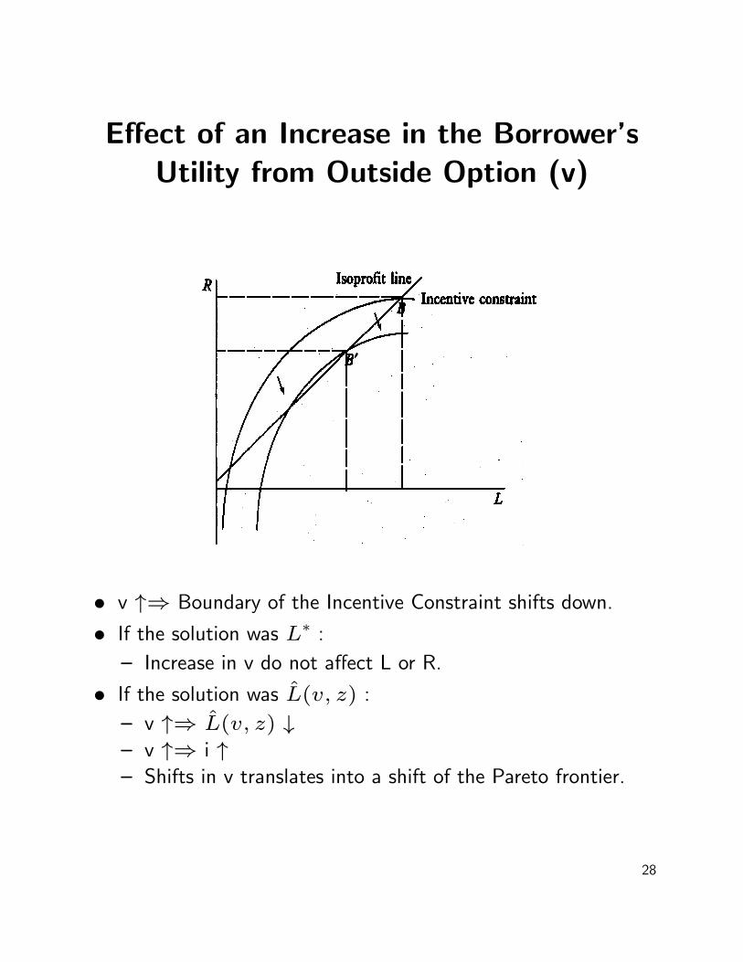
Effect of an Increase in the Borrower’sUtility from Outside Option (v)

• v ↑⇒ Boundary of the Incentive Constraint shifts down.

• If the solution was L∗ :

– Increase in v do not affect L or R.

• If the solution was L(v, z) :

– v ↑⇒ L(v, z) ↓– v ↑⇒ i ↑– Shifts in v translates into a shift of the Pareto frontier.

28

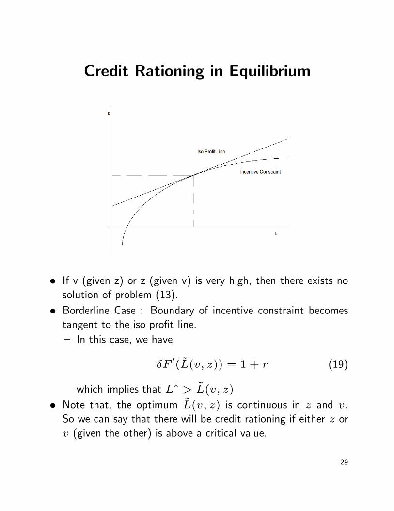
Credit Rationing in Equilibrium

• If v (given z) or z (given v) is very high, then there exists no

solution of problem (13).

• Borderline Case : Boundary of incentive constraint becomes

tangent to the iso profit line.

– In this case, we have

δF′(L(v, z)) = 1 + r (19)

which implies that L∗ > L(v, z)

• Note that, the optimum L(v, z) is continuous in z and v.

So we can say that there will be credit rationing if either z or

v (given the other) is above a critical value.

29

Summary

Equilibria which give more profit to the lender involve lower

overall efficiency, because credit rationing is more severe in such

equilibria as compared to the benchmark. Increased bargaining

power of lender thus reduce productivity. The reason is :

marginal rents accruing to the lender fall below social returns

from increased lending, the difference accounted for by the

incentive rents that accrue to the borrower.

The discussion can be summarised into the following proposition-

Proposition 4: There is credit rationing if z, the lender’s profit

(given v), or v, the borrower’s outside option (given z), is

above some threshold value. If rationing is present, a further

increase in the lender’s profit, or the borrower’s outside

option, leads to further rationing (i.e., a reduction in the

volume of credit) as well as a rise in the interest rate.

30

Social Surplus

• The social surplus is

g(L) = F (L)− (1 + r)L (20)

⇒ g′(L) = F

′(L)− (1 + r) (21)

• Note that F ′(L∗) = 1 + r and F ′′(.) < 0. So if L < L∗,

then F ′(L) > F ′(L∗). So we get g′(L) > 0∀L < L∗

• So we can say that if there is credit rationing, then social

surplus is less than the benchmark. As the rationing

increases, the social surplus decreases.

31

Endogenising the Borrower’s Utility fromthe Outside Option (v) : One Borrower,

Many Lender

• A drawback of partial equilibrium - The borrower’s utility from

the outside option (v) was taken to be exogenous.

• Now we describe the outside option which is available to a

defaulting borrower.

– In this case, we assume that there are more than one lender.

– Suppose the borrower got an offer (L,R) from a lender

L1, and the borrower defaulted. From that period on

wards, L1 will not offer him any loan, but the borrower can

ask for a loan to any other lender (say L2).

– We assume that the lender L2 screens the borrower and

offers another contract (L,R) with probability (1−p) and

offers nothing with probability p. p denotes the probability

that L2 will uncover the default commited by the borrower.

∗ The probability p will depend on the social network

structure of the lending community. Here, such network

structures is not analysed. We assume that p does not

change from one lender to another, and it is iid across

periods.

– If the borrower do not get a loan from L2, then he can

32

again ask for a loan to another lender (say L3), and the

story repeats.

• We confine our attention to the class of symmetric, stationary

SPNE, where each lender follows the trigger strategy of offering

the same contract (L,R) at all periods, if he fails to uncovers

that the the borrower has defaulted in the immediate past.

• Let v be the (ex-ante) expected utility the borrower gets from

the outside option.

• Let w be the payoff of the borrower in the one shot game, who

receives a contract (L,R) and complies. So, if he defaults,

he expects to attain a utility given by

pδv + (1− p)w• So, we must have

v = pδv + (1− p)w (22)

⇒ v =(1− p)w1− pδ

(23)

⇒ v = (1− ρ)w (24)

where ρ := p(1−δ)1−pδ is the scarring factor.Note that -

– limp→1

ρ = 1

– limδ→1

ρ = 0 if p ∈ (0, 1)

– limp→0

ρ = 0

33

Calculating v

• To determine v endogenously, we will use Proposition 4.

• Consider a given value of the lender’s profit (z) and any

arbitrary value of v for which the problem (13) has a solution.

• Now our objective is to force credit rationing in the model,

and then analyse the effect of an increase in the lenders’ profit

in such case. For this, we assume that the incentive constraint

of the borrower [equation (11)] holds with equality.

• Borrower’s utility in the one-shot game, given that he complies,

is given by -

F (L)− R= F (L)− δ[F (L)− v] [From equation (10)]

= (1− δ)F (L) + δv

• So, the borrower’s maximum utility, given that he complies,

will be given by

(1− δ)F (L(v, z)) + δv

• Let w(v; z) = (1− δ)F (L(v, z)) + δv

• So, we can say that v should satisfy

v = (1− ρ)w(v; z) (25)

Let φ(v; z) = (1 − ρ)w(v; z). Clearly, the optimal v will

be the fixed point of φ(.; z).

34

Equilibrium

• Once optimal v is obtained, then we can calculate equilibrium

offer L(v, z) for a fixed z. Hence we can use v to characterise

an equilibrium.

• Note that, as z is fixed, if v is above some threshold value

(say v), then there exists no solution. So we assume

φ(v; z) = 0 ∀ v ≥ v• φ(v; z) is decreasing in v -

– v ↑⇒ L(v, z) ↓.

– In this case L(v, z) < L∗ ∀v– So we can say, social surplus will decrease as v increases.

– As, we fixed z, so borrower’s utility will fall. As a

consequence, φ(.; z) will decrease.

• There is an unique fixed point - v∗ in the diagram if there is

an intersection with 45◦ line before the point of discontinuity.

Otherwise, no symmetric equilibrium exists.

35

Effect of Change in Scarring Factor (ρ)in the Equilibrium

• Let z be an upper bound of z, for which the problem has a

solution.

• ρ ↑⇒ φ(v; z) ↓, but the discontinuity point of φ(v; z) will

not change (since w(v, z) is independent of ρ).

• So we get the following proposition -

Proposition 5: Suppose z ≤ z. There is a unique

equilibrium in the credit market provided ρ is greater than

some threshold value ρ∗, i.e., either the borrowers are

sufficiently patient, or the probability of detection is high

enough.

• Note that ρ∗ will depend on z.

36

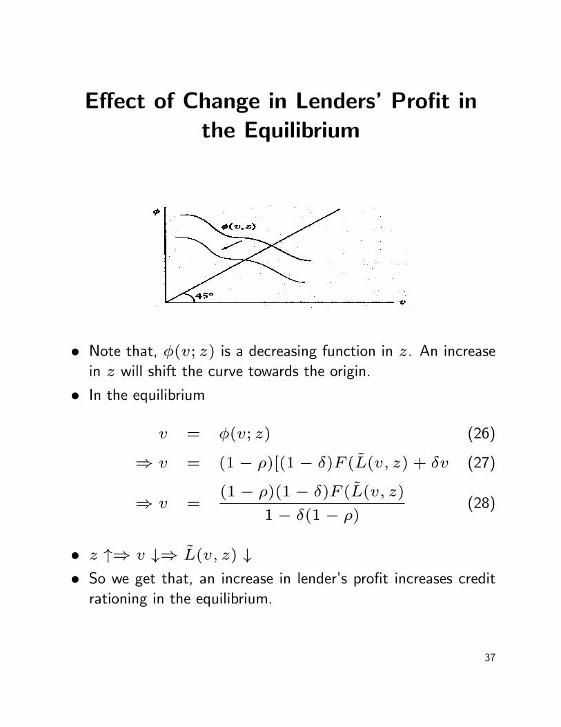
Effect of Change in Lenders’ Profit inthe Equilibrium

• Note that, φ(v; z) is a decreasing function in z. An increase

in z will shift the curve towards the origin.

• In the equilibrium

v = φ(v; z) (26)

⇒ v = (1− ρ)[(1− δ)F (L(v, z) + δv (27)

⇒ v =(1− ρ)(1− δ)F (L(v, z)

1− δ(1− ρ)(28)

• z ↑⇒ v ↓⇒ L(v, z) ↓• So we get that, an increase in lender’s profit increases credit

rationing in the equilibrium.

37