ABSTRACTPrototyping and design of hydro turbines can be expensive and time consuming. Developing accurate theoretical
analysis of a hydro turbine is essential to reducing time and money spent in design. In this report we discuss themethods and results of analyzing a small cross flow hydro turbine. This analysis is used to accurately estimatethe torque and power output of the turbine. We accomplished this by using an iterative process of comparing thetheoretical results to the experimental results. We identified several sources of error in our first correlation thatneeded to be corrected. These included using a much larger minor loss coefficient than previously anticipatedand assuming that only 75% of the water jet stream actually enters the turbine. After applying these discoveredfactors we were able to accurately predict the performance of the hydro turbine. We found that our theoretical datamainly aligned with our experimental data within the error of systematic uncertainty. These results show that theperformance of a cross flow turbine can be accurately predicted but that experimental data might be necessary toidentify unanticipated error factors.
Nomenclature
T TorqueW Relative velocityP PressureV Absolute velocityQ Volumetric flowrateF ForceK Minor loss coefficientWt WeightU Reference frame velocityN Number of vanesE Power
d Diameterr Radiusm Mass flow rateg Gravitational constanta Acceleration constants Kinematic position of a particle
v Kinematic velocity of a particlet Timef Coefficient of frictionz Height
f Subscript. refers to frictionspool Subscript, refers pulleytur Subscript, refers to turbine
1 IntroductionTurbines are used throughout the world but are costly to prototype at a large scale. The turbine in question is a Cross
Flow or Banki-Mitchell Turbine. The Cross Flow Turbine was originally designed by an Australian engineer named A.G.MMitchell in 1903. It was later developed upon by Donat Banki through series of publications between the years of 1917 and1919 [1]. Then in the year 1922 a German entrepreneur named Fitz Ossberger contacted Mitchell. During that year theydesigned and patented the Ossberger Turbine wheel. It was refined over the next decade with numerous refinements and theOssberger turbine went into production in 1933 [2]. Ossberger today is the leading manufacture for Cross Flow Turbines.
A Cross Flow turbine is different than other Turbines available today. The water enters the turbine making contact witha blade on the turbine and then continues though to exit hitting another blade as the fluid exits the turbine. With the design ofthe turbine it has some advantages over the other readily available turbines in today’s market. One of the major advantagesis the wide variety of operating conditions in which it can perform and maintain the same efficiency. This allows places withlow head differences and slow flow rates to be able to create energy where other turbines cannot. They typically can operateon head differences of 5.75 feet H20 all the way up to 675 feet H20 of head difference. This is the same for flow rate a CrossFlow Turbine can operate on flows between 10.5 gallons per second up to 1320 gallons per Second [3]. Another advantage tothe turbines is the amount of maintenance required. The Cross Flow Turbine has very little maintenance required to keep itoperational. For example is that it has low maintenance bearings, very little moving parts and theoretically self cleaning [2].The only disadvantage of this style of turbine is when the flow rate and the head difference are higher than stated there aremore beneficial choices.
1.1 ObjectivesFor this project we were trying to accurately estimate the torque and power output of a crossflow hydro turbine. This is
accomplished by theoretically analyzing the turbine and comparing our theoretical results to results gathered experimentally.
3
(a) Piping schematic (b) A cross flow turbine with impinging jet
Fig. 1: Cross-flow urbine testing schematics showing the pulley and turbine with impinging jet, and the piping systemlocations and fittings used in estimating the jet
This is useful because designing and testing a full size turbine can have extremely high costs involved depending on the sizeof turbine being designed. Being able to scale the design down to an economical size will be beneficial. We also applied ourknowledge of writing technical reports to clearly communicate the methods and results of the project.
2 Hydro Turbine TheoryHydroturbines are used to generate power through deflection of water on vanes which does mechanical work on a shaft.
The fluid mechanic theory that governs this process is the conservation of angular momentum. When momentum is changed,a force or torque is produced. This stems from Newton’s Second Law, F = dmV
dt , where force is equal to the change inmomentum with respect to time. To analyse a turbine, the test setup shown schematically in Fig.1 will be referenced. Inorder to calculate the torque and power the turbine is capable of producing, we must first estimate the velocity of the jet as itexits the nozzle.
2.1 Pipe Loss AnalysisThe general 1-D energy equation for pipe flow between two points is
P1
ρ+
12
V 21 +ρgz1−
12
f`
D1V 2
1 −12 ∑KV 2
1 =P2
ρ+
12
V 22 +ρgz2 (1)
and the application of conservation of mass yields
A1V1 = A2V2 (2)
D21V1 = D2
2V2 (3)
Which may be used in combination to solve for the velocity at the nozzle exit. Picking z2 as a datum and working in gagepressure, the equation for the jet velocity becomes
4
V2 =
√√√√√√ 2(
P1ρ+ρgz1
)1+(
D2D1
)4 [f `
D +∑K−1] (4)
This equation contains the friction factor f and the minor loss coefficients ∑K. The latter of which may be estimatedusing tabulated values. To find the friction factor if we assume the flow is turbulent, we may make use of the Haaland formulawhich represents the turbulent portion of the Moody Chart [4].
1√f=−1.8log
[(ε/D3.7
)1.11
+6.9ReD
](5)
The Haaland formula requires knowledge of the Reynold’s number, which depends on the velocity of the fluid in the pipe.As such a guess for the pipe velocity must be made, and the friction factor solved iteratively. This is done easily withnumerical iteration and may be checked against the measured pressure in the pipe. The estimated velocity of the jet will beused to estimate the theoretical torque and power curves for the specific turbine.
2.2 Theoretical Torque and Power AnalysisThe hydro turbine converts the kinetic energy of an impinging water jet into mechanical work which is used to turn a
shaft, thereby producing power. In analyzing this conversion of energy, the following assumptions must be made
1. The water behaves as an incompressible fluid2. The fluid properties remain constant3. The difference in elevation across the turbine is negligible4. The turbine operates in steady state5. The effects of viscosity are neglected6. All of the water enters and exits the turbine
To find the torque and power produced by the turbine, the absolute velocity of the water entering and leaving the turbineis required, which requires knowledge of the water velocities relative to the wheel itself. We will have to solve for thevelocities, the entrance angle, and the exit angles of the water jet.
We begin with relative velocities, using the non-deforming control volume in Fig. 2a. The control volume is allowed torotate at the same rate as the wheel, and as such, sees no work done on the wheel and no power produced.
To find relative velocities W1 and W2, the Bernoulli equation [4] may be used
P+12
V 2 +gz = constant (6)
Inserting the relative velocities and utilizing assumption 3 to neglect the potential energy terms
P1 +12
W 21 = P2 +
12
W 22 (7)
and recognizing that the pressure of a free jet is atmospheric, such that P1 = P2 we find that W1 =W2, and the relativevelocities are equal.
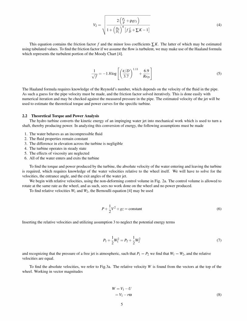
To find the absolute velocities, we refer to Fig.3a. The relative velocity W is found from the vectors at the top of thewheel. Working in vector magnitudes
W =V1−U
=V1− rω (8)
5
(a) Rotating (b) Fixed
Fig. 2: Fixed and rotating control volumes used in torque and power analysis. Both are non-deforming, but only CV2 isacted on by a torque. Notice that the jet exit angle is different for each situation
Again working in magnitudes and performing component-wise vector addition
V2 =
√(U−W cosβ)2 +(−W sinβ)2
=
√(rω−W cosβ)2 +(−W sinβ)2 (9)
To solve for the dynamic angle θ, we reference Fig.3b and make use of the law of cosines
α = cos−1(
U2−W 2−V 22
−2WV2
)(10)
Where α = θ−β
θ = β+ cos−1(
U2−W 2−V 22
−2WV2
)(11)
With the velocities and angles known we may turn our attention towards finding the torque. Referring to the fixed,non-deforming control volume seen in Fig. 2b, the Reynold’s Transport Theorem [4] is used to solve for the torque
∑T =∂
∂t
∫cv
ρ(~r×~v)dV– +∫
csρ(~r×~v)(~V · n)dA (12)
6
(a) The velocity vectors relevant to the cross flow (b) The vector triangle used to solve for the dynamic angle θ
Fig. 3: Velocity vector diagrams used to solve the kinematics of the turbine flow
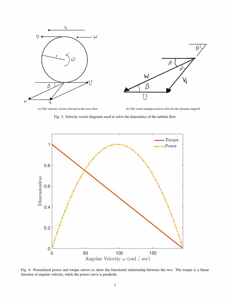
Fig. 4: Normalized power and torque curves to show the functional relationship between the two. The torque is a linearfunction of angular velocity, while the power curve is parabolic
7
Which simplifies to
∑T = ∑out
m Vθ−∑in
m Vθ (13)
Recognizing that the mass flowing into the CV must equal the mass leaving the CV, the general torque equation becomes
T =−mr (V2 cosθ−V1) (14)
The direction of the torque was assumed to match that of the angular velocity of the wheel, and as such the negative in Eqn.(14) tells us that the device operates as a turbine, extracting work from the fluid.
To get an idea of the functional relationship between angular velocity ant torque, T = f (ω), we substitute the make useof the Pythagorean identity
T =−mr[cosθ
(rω
2−2rωW cosβ+W 2)1/2+W + rω
](15)
Which shows that torque is a linear function of angular velocity.
To find the power, we simply multiply the torque by angular velocity which means that power is proportional to thesquare of velocity, E ∝ ω2. The power equation used in generating the theoretical curve in this article is
E =−mrω(V2 cosθ−V1) (16)
The preceding discussion showed the derivation of functional relationships for torque and power as functions of wheelangular velocity. The assumptions made in the derivations mean that the relationships actually describe the maximumtheoretical values extracted from the fluid, while the potential to extract work and power from the turbine will be considerablylower. To compare our resulting equations, we will solve for the torque and power experimentally as well.
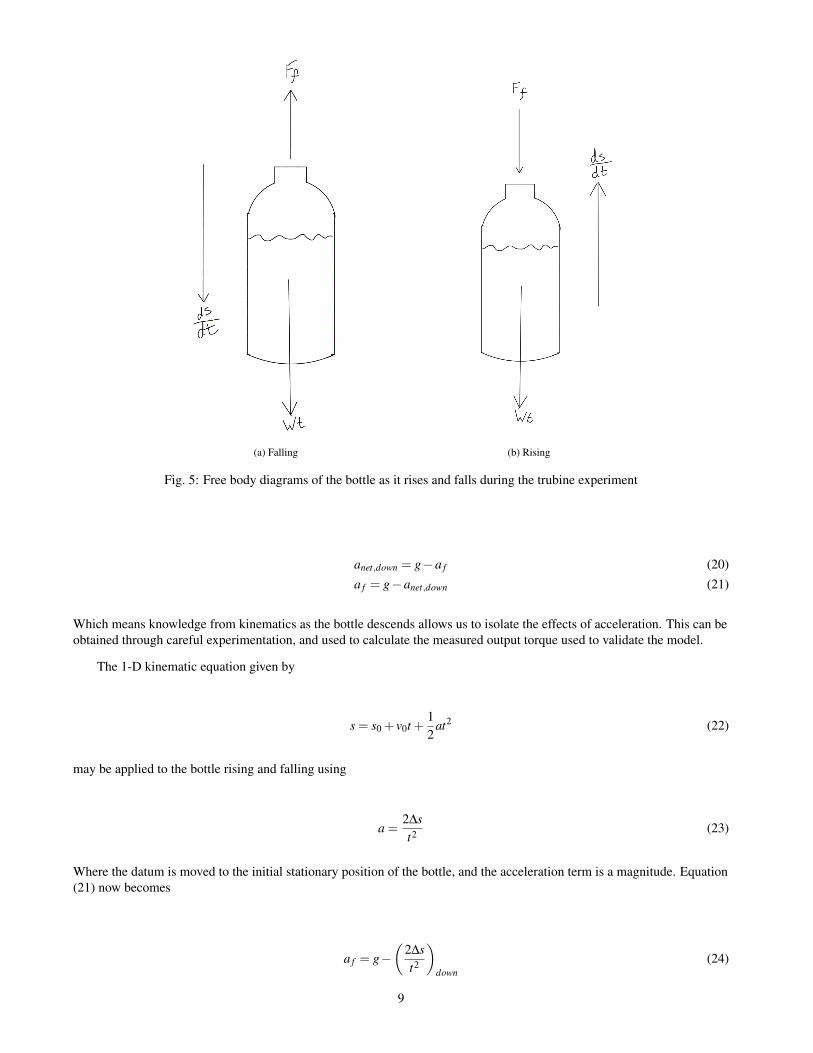
2.3 Experimental Torque and Power AnalysisThe losses associated with friction can be found from the free-body-diagram in Fig.5a.
∑~F = m~a
Ff −Wt = m~a (17)
This equation may be solved for the frictional force to find that
Ff =Wt−manet,down (18)
Or, alternatively noting that the two forces acting on the bottle are in opposite directions and F = ma, we split theacceleration term into two components.
Ff −Wt = m(a f −g) (19)
Which means that the acceleration terms are related by the equations
8
(a) Falling (b) Rising
Fig. 5: Free body diagrams of the bottle as it rises and falls during the trubine experiment
anet,down = g−a f (20)a f = g−anet,down (21)
Which means knowledge from kinematics as the bottle descends allows us to isolate the effects of acceleration. This can beobtained through careful experimentation, and used to calculate the measured output torque used to validate the model.
The 1-D kinematic equation given by
s = s0 + v0t +12
at2 (22)
may be applied to the bottle rising and falling using
a =2∆st2 (23)
Where the datum is moved to the initial stationary position of the bottle, and the acceleration term is a magnitude. Equation(21) now becomes
a f = g−(
2∆st2
)down
(24)
9
(a) A plot of the dynamic angle of the jet exiting the turbine when observedfrom a fixed frame of reference was generated using Eqtn. (11). Noticethe plot ends at 180, which seems physically unlikely to happen in theexperiment.
(b) A plot of the relationship between the wheel tangential velocity, therelative fluid velocity, and the absolute exit velocity. See Eqtns. (8-9) forthe relative and exit velocities.
Fig. 6: Kinematic Plots
Having the acceleration of friction in hand, we may calculate the measured torque from Torque = Force×Distance
T = rspool m(g+a f ) (25)
The angular velocity can be related to the linear velocity of the string through
dzdt
= rspoolω (26)
The power may be calculated using
P = T ω (27)
10
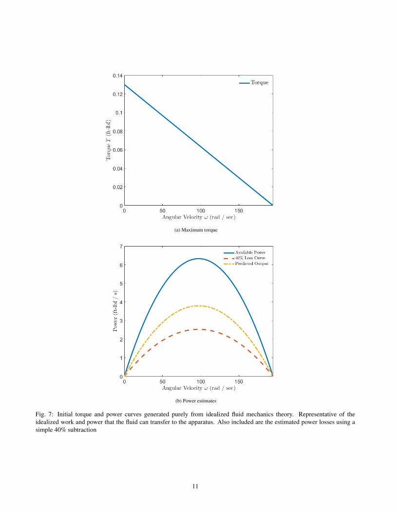
(a) Maximum torque
(b) Power estimates
Fig. 7: Initial torque and power curves generated purely from idealized fluid mechanics theory. Representative of theidealized work and power that the fluid can transfer to the apparatus. Also included are the estimated power losses using asimple 40% subtraction
11
Table 1: Predicted maximum turbine power output and total power available from the change in fluid momentum
Power E ft-lbf/s
Available Fluid Power 6.327
1st Estimated Output 3.797
2nd Estimated Output 1.918
Table 2: Mean weight and friction forces for the experiment
Weight (lbf) 0.568
Friction Force(lbf) 0.531
Ratio 0.948
Table 3: Estimated values between iterations. These were the three values that adjusted the theory curves in line with theexperimental results
Jet Velocity (ft/s) Minor Loss Coefficient ∑K Modifying Factor γ
1st Estimate 27.88 30.3 1
2nd Estimate 20.52 27.75 .76
Ratio 0.74 9.16 0.76
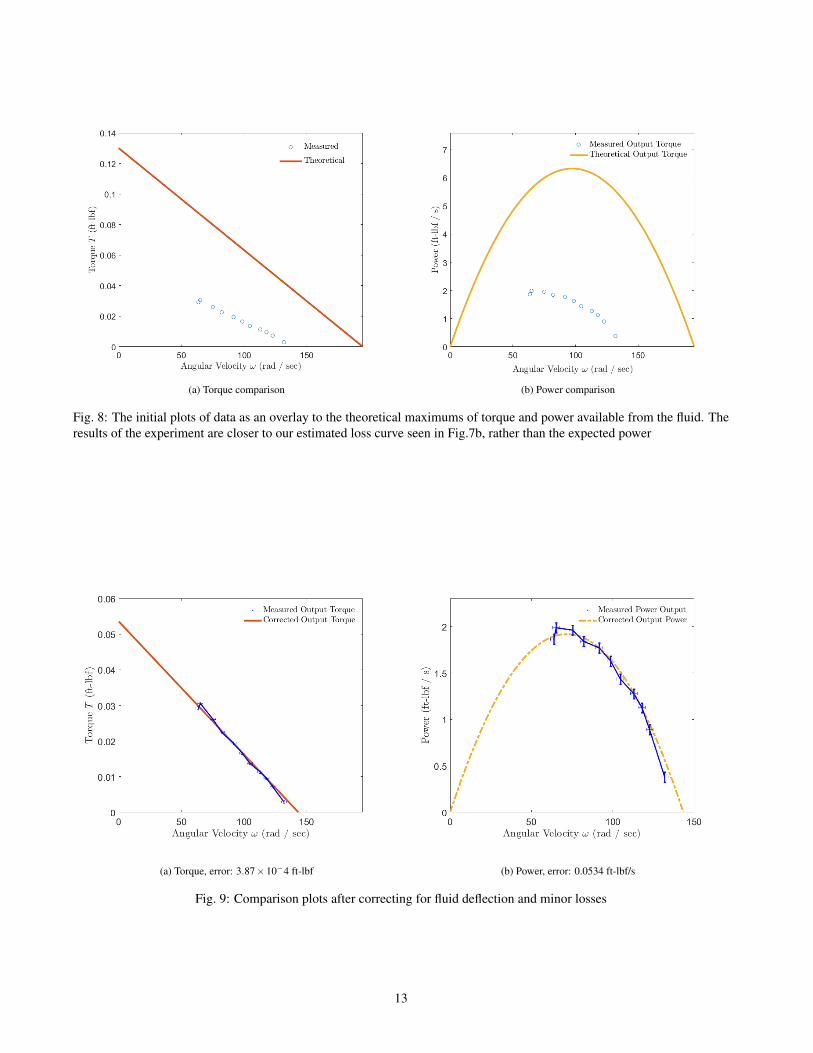
3 ResultsThe results of the experiment are shown in Fig.8, where it can be seen that the assumptions made in the analysis were
insufficient to predict the power output of a turbine. It was noted during the experiment that not all of the water went into theturbine, making assumption 6 invalid. In actually a percentage of the fluid enters the turbine which may be estimated by theopen surface area of the turbine circumference. The ratio of open surface to vane surface over the circumference is
λ = 1− bNπDtur
(28)
The value of λ is approximately 75%, and it can be used as a corrective factor with Eqtns. (14) and (16) to account for thisdifference. They become
T =−λmr (V2 cosθ−V1) (29)E =−λmrω(V2 cosθ−V1) (30)
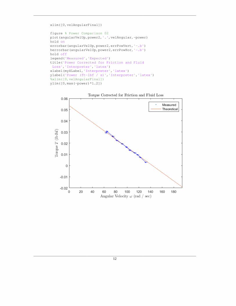
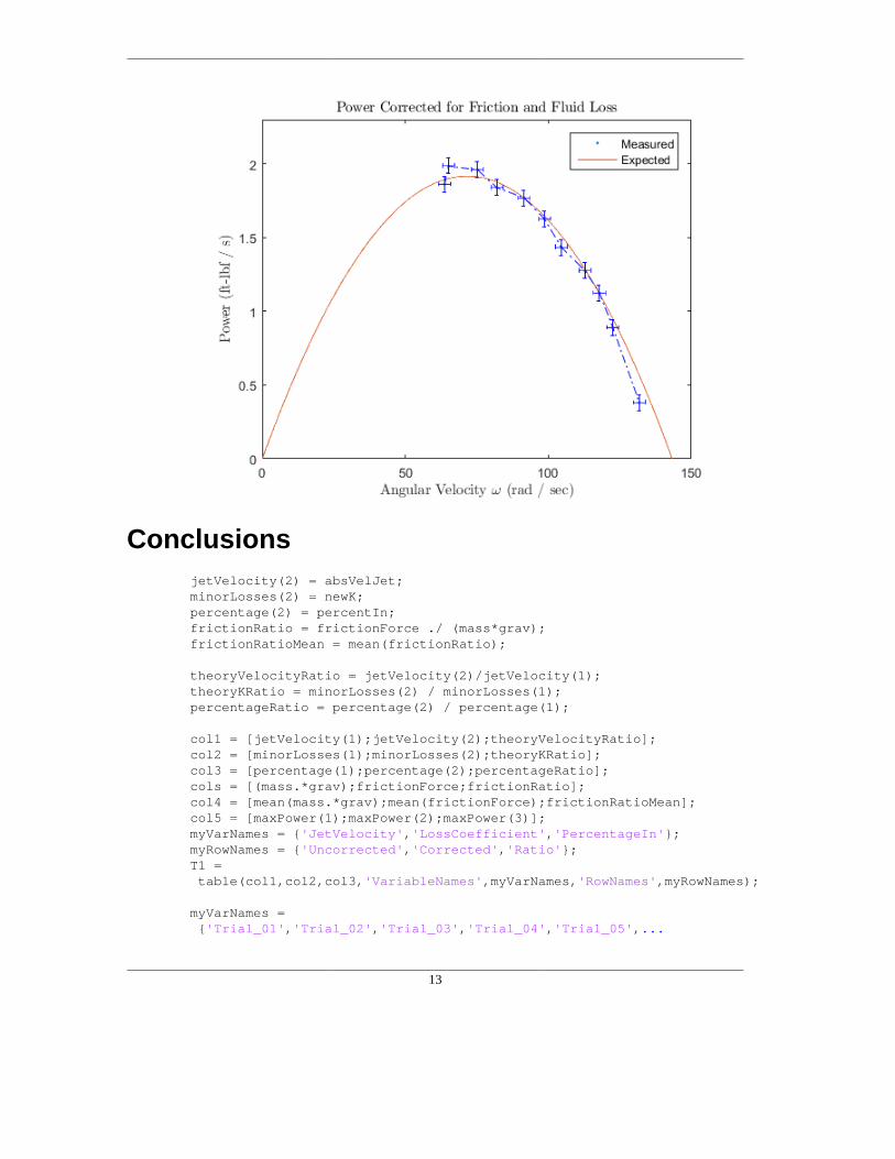
While this corrective factor will bring the theoretical solution more in line with the measured results, our initial estimatesfor exit velocity are of concern also. The experimentally derived jet velocity was 20.66 ft/s which was only 74% of our firstestimated value. Equation 1 can be solved for the minor loss coefficient ∑K to feed back into the theoretical calculations.This was done using Matlab computation software, which resulted in the minor loss coefficient increasing by a factor of 9.Re-evaluating the code used to generate the theoretical curves results in the plots shown in Fig.9.
12
(a) Torque comparison (b) Power comparison
Fig. 8: The initial plots of data as an overlay to the theoretical maximums of torque and power available from the fluid. Theresults of the experiment are closer to our estimated loss curve seen in Fig.7b, rather than the expected power
Fig. 9: Comparison plots after correcting for fluid deflection and minor losses
13
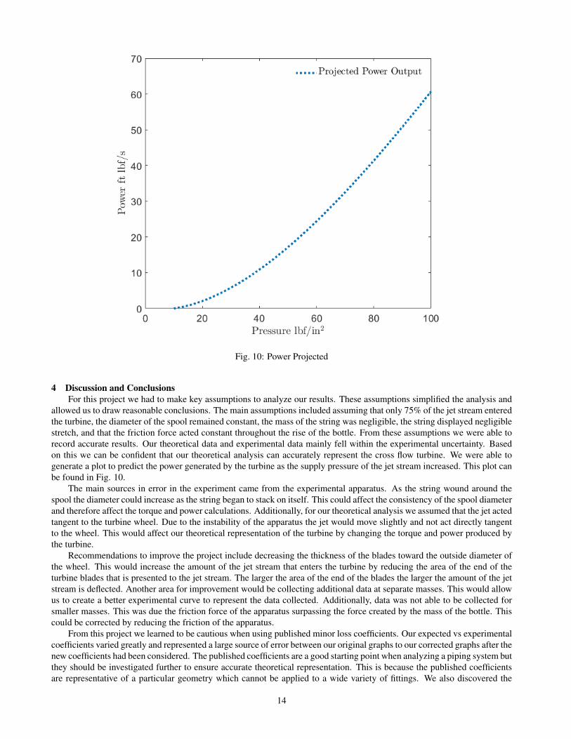
Fig. 10: Power Projected
4 Discussion and ConclusionsFor this project we had to make key assumptions to analyze our results. These assumptions simplified the analysis and
allowed us to draw reasonable conclusions. The main assumptions included assuming that only 75% of the jet stream enteredthe turbine, the diameter of the spool remained constant, the mass of the string was negligible, the string displayed negligiblestretch, and that the friction force acted constant throughout the rise of the bottle. From these assumptions we were able torecord accurate results. Our theoretical data and experimental data mainly fell within the experimental uncertainty. Basedon this we can be confident that our theoretical analysis can accurately represent the cross flow turbine. We were able togenerate a plot to predict the power generated by the turbine as the supply pressure of the jet stream increased. This plot canbe found in Fig. 10.
The main sources in error in the experiment came from the experimental apparatus. As the string wound around thespool the diameter could increase as the string began to stack on itself. This could affect the consistency of the spool diameterand therefore affect the torque and power calculations. Additionally, for our theoretical analysis we assumed that the jet actedtangent to the turbine wheel. Due to the instability of the apparatus the jet would move slightly and not act directly tangentto the wheel. This would affect our theoretical representation of the turbine by changing the torque and power produced bythe turbine.
Recommendations to improve the project include decreasing the thickness of the blades toward the outside diameter ofthe wheel. This would increase the amount of the jet stream that enters the turbine by reducing the area of the end of theturbine blades that is presented to the jet stream. The larger the area of the end of the blades the larger the amount of the jetstream is deflected. Another area for improvement would be collecting additional data at separate masses. This would allowus to create a better experimental curve to represent the data collected. Additionally, data was not able to be collected forsmaller masses. This was due the friction force of the apparatus surpassing the force created by the mass of the bottle. Thiscould be corrected by reducing the friction of the apparatus.
From this project we learned to be cautious when using published minor loss coefficients. Our expected vs experimentalcoefficients varied greatly and represented a large source of error between our original graphs to our corrected graphs after thenew coefficients had been considered. The published coefficients are a good starting point when analyzing a piping system butthey should be investigated further to ensure accurate theoretical representation. This is because the published coefficientsare representative of a particular geometry which cannot be applied to a wide variety of fittings. We also discovered the
14
importance of iterative calculations. We found it necessary to use multiple iterations to calculate our minor loss coefficientand our jet velocities as well as using multiple iterations when adjusting our theoretical data to our experimental data. Wewere able to decrease the time to perform these calculations by using mathematical software but these calculations wouldprove very time consuming otherwise.
Overall we were able to accurately match our theoretical analysis of the turbine to our experimental results. Thisprocess helped us to understand the importance of theoretical analysis and confirm that experimental results cannot replacetheoretical analysis. The project also helped us to understand the complexities that are present in actual applications thatmay be overshadowed in general theoretical analysis.
References[1] Walseth, E. C., 2009. Investigation of the flow through the runner of a cross-flow turbine. Web. PDF, Accessed 2016.[2] Ossberger, 2015. The original ossberger turbine. Web. PDF, Accessed 2016.[3] Renewable First. Crossflow turbines. Web. Accessed 2016.[4] Munson, B. R., 2012. Fluid Mechanics 7e. Wiley Higher Ed.
15
Table 4: Measurement uncertainty associated with the experimental torque and power calculations
Measurement Uncertainty Ω Units
Mass ±3.426×10⁻⁶ slug
Gravity ±0.3281 ft/s2
String Length ±5.208×10⁻³ ft
Time ±1.00×10⁻⁴ sec
Length ±6.562×10⁻⁴ ft
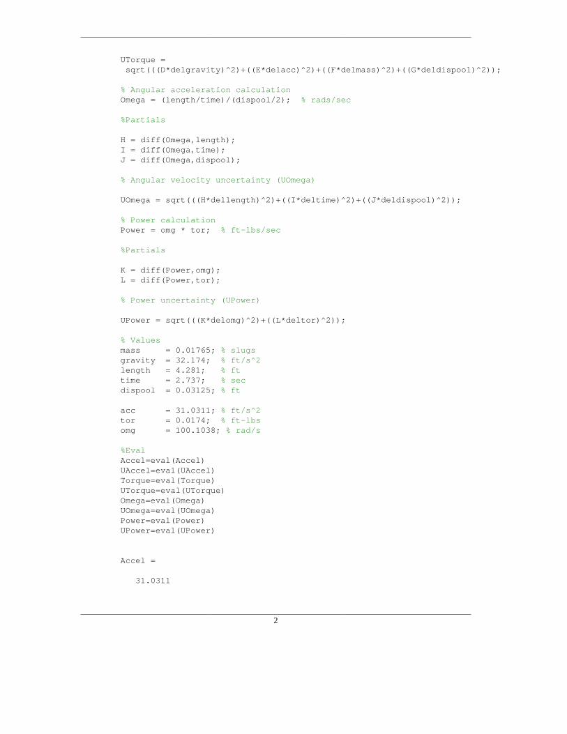
A UncertaintyThe systematic uncertainty in this experiment was introduced by the bottle mass, gravity, string length, time, and spool
diameter measurements. The values used in the calculations are shown in Tab.4.We used the partial differentiation method of finding uncertainty using the following equation.
Ωy =
√n
∑i=1
(∂y
∂xiΩi
)2
(31)
Uncertainty calculations were performed on the experimental Eqtns. (21) and (25-27). The calculations were done in thefollowing manner, first deriving the relevant equation with respect to the appropriate elements.
A.1 Acceleration Partials
∂a∂g
= 1 (32)
∂a∂∆z
=− 2∆t2 (33)
∂a∂∆t
=4∆z∆t3 (34)
A.2 Torque Partials
∂T∂m
= (a f +g)Dspool
2(35)
∂T∂g
=Dspoolm
2(36)
∂T∂a f
=Dspoolm
2(37)
∂T∂Dspool
=(a f +g)m
2(38)
16
A.3 Angular Partials
∂ω
∂∆z=
2∆tDspool
(39)
∂ω
∂∆t=−2∆z
∆t2Dspool(40)
∂ω
∂Dspool=−2∆z
D2spool∆t
(41)
A.4 Power Partials
∂E∂T
= ωup (42)
∂E∂ωup
= T (43)
Ωa f =
√(∂a f
∂g×Ωg
)2
+
(∂a f
∂∆z×Ω∆z
)2
+
(∂a f
∂∆t×Ω∆t
)2
(44)
ΩT =
√(∂T∂m×Ωm
)2
+
(∂T∂g×Ωg
)2
+
(∂T
∂Dspool×ΩDspool
)2
+
(∂T∂a f×Ωa f
)2
(45)
Ωω =
√(∂ω
∂ω×Ωω
)2
+
(∂ω
∂∆t×Ω∆t
)2
+
(∂ω
∂Dspool×ΩDspool
)2
(46)
ΩE =
√(∂E∂T×ΩT
)2
+
(∂E
∂∆ω×Ω∆ω
)2
(47)
17
Table 5: Uncertainty results
Measurement Uncertainty Ω Units
Acceleration ±0.3281 ft/s2
Torque ±3.8774×10−04 ft-lbf
Angular Velocity ±2.1054 rad/s
Power 0.0534 ft-lbf/s
18
1
Table of ContentsHydro Turbine Project - Theoretical ....................................................................................... 1Store the nominal variables ................................................................................................... 1Store the estimated variables ................................................................................................. 1Preliminary Calculations ....................................................................................................... 1Part 2 of the analysis is all about torque and momentum ............................................................ 2Produce the initial plots before carrying out the experiment ........................................................ 3Store the collected data ........................................................................................................ 7Post Experiment Calculations ................................................................................................ 81st Post-Experiment Plots ..................................................................................................... 8Begin the Refinement Process ............................................................................................. 102nd Post-Experiment Plots .................................................................................................. 11Conclusions ...................................................................................................................... 13
Store the estimated variablesK = [ 1.5, 1.5, 0.03 ]; % ignores the regulatorsumK = sum(K);rough = 0.06e-3; %[in]vel1 = 5.1; % guessed economic velocity[ft/s]percentIn = 1;diamPipe = 0.5 / 12; %[ft] Just ran in and looked at itpipeLength = 224/12; %[ft] " "deltaZ = 4/12; %[ft] " "
Preliminary CalculationsNeed to estimate the absolute velocity of the jet.
B Matlab Code
19
2
relativeRough = rough / diamPipe; % for getting on the moody chartscheck = 1e6; % for the while loopsyms frictionwhile abs(check) > (.01*144) % 1 percent of the 10 psi vel2 = (diamPipe / diamJet)^2 * vel1; % conservation of mass Re = densityH20 * vel1 * diamPipe / viscH20; eqtn = 1/sqrt(friction) == -1.8 * ... % correlation from munson (turb) log10( ( relativeRough/3.7 )^1.11 + 6.9/Re ); fric = vpasolve(eqtn,friction,.002); fric = double(fric); deltaP = densityH20 * ( 0.5 * ( vel2^2 - vel1^2 + fric * pipeLength... * vel1^2 / diamPipe + sumK * vel1^2 ) ) + densityH20 * grav * deltaZ; check = deltaP - pressSupp; vel1 = vel1+.01;endvel1 = vel1 - .01;absVelJet = vel2; % Here's are calculated velocity from theoryjetVelocity(1) = absVelJet;minorLosses(1) = sumK;frictionFactor(1) = fric;percentage(1) = percentIn;
Part 2 of the analysis is all about torque andmomentum
% fill an array for our domain of plotsvelAngularFinal = absVelJet / radiWheel; % Torque and power should zero herevelAngular = linspace(0,velAngularFinal,1000); %[rad/sec]
% use the law of cosines to find the angle from the "dynamic angle" C = radiWheel .* velAngular; B = absVelJet - C; A = absVelExit; myLength = ( C.^2 - A.^2 - B.^2 ) ./ ( -2 .* A .* B ); angleDynamic = angleBlade + acos( myLength );
3
% Here are the torque and power calculations. Only some of the water enters% the wheel.
% The plot of torque (need the ordinate to be flipped for work out)figureplot(velAngular,-torque)title('Torque','Interpreter','latex')xlabel(myXLabel,'Interpreter','latex')ylabel('Torque $T$ (ft-lbf)','Interpreter','latex')xlim([0,velAngularFinal])
% The expected max, loss, and net power we expectfigureplot(velAngular,-power,velAngular,loss,velAngular,powerExpected)
% Normalized Torque and Power Plots to check the theoryfigureplot(velAngular,-torqueNorm, velAngular, -powerNorm)xlabel(myXLabel,'Interpreter','latex')ylabel('Dimensionless')legend('Torque','Power')title('Normalized Power and Torque','Interpreter','latex')xlim([0,velAngularFinal])ylim([0,1.1])
5
6
7
Grab the critical values from the power curve
fprintf('The maximum power output is expected to be %.2f ft-lbf.\n',maxPower(2))fprintf('The optimal angular speed is %.2f rads/sec.\n',velAngular(optVelAngular(2)))
The maximum power output is expected to be 3.80 ft-lbf.The optimal angular speed is 97.23 rads/sec.
Store the collected datalengthString = 51.375/12; % [ft]mass = 6.85218e-5 * [ 445.4,... %[slugs]462.2,...394.5,...337.6,...289.4,...245.8,...203.1,...166.9,...140.5,...106.4,...42.1 ];
figure % Power Comparison 01plot(angularVelUp,power2,'o',velAngular,-power)legend('Measured','Expected')title('Uncorrected Power Comparison','Interpreter','latex')xlabel(myXLabel,'Interpreter','latex')ylabel('Power (ft-lbf / s)','Interpreter','latex')xlim([0,velAngularFinal])ylim([0,max(-power)*1.2])
10
Begin the Refinement ProcessSome of the code here is a copy-paste from up above. Start by finding the experimental minor loss coef-ficients.
syms sumK2vel2 = absVelJet2; % Set this to the experimental valuevel1 = (diamJet / diamPipe)^2 * vel2;
% Set up the old deltaP equation to be solved for K this timeeqtn = pressSupp == densityH20 * ( 0.5 * ... ( vel2^2 - vel1^2 + fric * pipeLength * vel1^2 ... / diamPipe + sumK2 * vel1^2 ) ) + densityH20 * grav * deltaZ;newK = vpasolve(eqtn,sumK2);newK = double(newK);
Now re-solve the friction factor and jet velocity estimate
% use the law of cosines to find the the "dynamic angle" C = radiWheel .* velAngular; B = absVelJet - C; A = absVelExit; myLength = ( C.^2 - A.^2 - B.^2 ) ./ ( -2 .* A .* B ); angleDynamic = angleBlade + acos( myLength );
% Recalculate the torque and power, use the better ratio of what's going inpercentOut = thick * numVanes / ( pi * diamWheel );percentIn = 1 - percentOut;
% use the law of cosines to find the the "dynamic angle" C = radiWheel .* velAngular; B = velProjected - C; A = absVelExit; myLength = ( C.^2 - A.^2 - B.^2 ) ./ ( -2 .* A .* B ); angleDynamic = angleBlade + acos( myLength );
figureplot(P1/144,maxPowerProjected)title('Projected Power Based on Inlet Pressure','Interpreter','Latex')xlabel('Pressure lbf/in$^2$','Interpreter','latex')ylabel('Power ft lbf/s','Interpreter','latex')
16
Published with MATLAB® R2015b
1
clear allclose allclc
% Northrop% Thermal Fluids Project Uncertainty
syms mass gravity length time dispool acc omg tor pow
Table 1: Testing plan for the Pelton wheel water turbine
Objective Determine the performance of a small water turbine (Pelton wheel).
Power as a function of angular velocity
Torque as a function of angular velocity
Assumptions
Fluid is incompressible fluid
Constant Fluid Properties
Difference in elevation across the wheel is negligible
Turbine operates steadily
Water behaves as an inviscid fluid within the wheel
Frictional power losses are linearly related to angular speed
Torque caused by friction is a constant
Hazards and PPE PPE
Everyday clothing
Place to warm up
Optional eyewear
Flip-flops suggested
Tools required
Test stand
Smart phone with video capability
Some kind of Tri-Pod (optional)
Timer
Calipers
Sharpie
Rule
Weight scale
Fluid container (bucket)
Thermometer or access to local temperature data
Test Setup, Required
Environment
Environment must be outdoors with a common garden hose faucet. Preferably on a hot day
Testing apparatus has been built by previous classes of engineers and is photographed below
C Testing Plan
38
1. Attach end of hose to faucet 2. Ensure that the bottle is full of liquid with known density
Procedure (Execution
and Data Collection)
1. Take caliper measurements of:
a. Turbine diameter
b. Turbine bearing diameter
c. Jet diameter (if possible)
d. Spool diameter
e. Pulley bearing diameter
2. Mark a long length on the string using the sharpie with a mark just
above the bottle cap
a. Measure the length between the marks
3. Cover jet outlet and position bucket to collect the flow.
4. Start the timer and flow simultaneously. Measuring the time it takes to
fill the bucket and record for mass flowrate calculations. Record the
time and the volume collected. Turn flow off.
5. Remove the cover and bucket. Reset the apparatus.
6. Fill the water bottle with water. 7. Test the turbine. Empty incremental amounts of water until the water
jet is just able to raise the bottle. 8. Weigh the water bottle 9. Set the smartphone camera up on the tri-pod pointed at the full
apparatus. Ensure that the bottle is in the frame.
a. Begin recording low resolution video.
10. Turn on the flow. Start timer.
11. When the low mark reaches the pulley, turn the flow off.
a. Record time
12. Let the bottle fall
a. Record time
13. Stop and save the trial video to keep file size low
14. Repeat steps 8a-11 a total of 4 trials at each weight
15. Remove ~10mL from the bottle 16. Return to step 8 a total of 10 times
Data Analysis &
Conclusion Need:
1. Flowrate from volume filled / time to fill 2. Jet velocity from flowrate * jet area 3. Work from bottle weight * distance traveled 4. Power from weight * distance traveled / elapsed time
a. Frictional losses found from when bottle drops by gravity b. Power produced is calculation on rise – calculation on fall