B IVARIATE G ENERALIZED E XPONENTIAL D ISTRIBUTION Debasis Kundu Department of Mathematics and Statistics Indian Institute of Technology Kanpur Part of this work is going to appear in J. Mult. Anal. . – p.1/25
Transcript
BIVARIATE GENERALIZED EXPONENTIAL
DISTRIBUTION
Debasis KunduDepartment of Mathematics and Statistics
Indian Institute of Technology Kanpur
Part of this work is going to appear in J. Mult. Anal.
. – p.1/25
OUTLINE OF THE TALK
Univariate Generalized Exponential Distribution
Basic Properties
Bivariate Generalized Exponential Distribution
Properties
Estimation
Generalizations
. – p.2/25
OUTLINE OF THE TALK
Univariate Generalized Exponential Distribution
Basic Properties
Bivariate Generalized Exponential Distribution
Properties
Estimation
Generalizations
. – p.2/25
OUTLINE OF THE TALK
Univariate Generalized Exponential Distribution
Basic Properties
Bivariate Generalized Exponential Distribution
Properties
Estimation
Generalizations
. – p.2/25
OUTLINE OF THE TALK
Univariate Generalized Exponential Distribution
Basic Properties
Bivariate Generalized Exponential Distribution
Properties
Estimation
Generalizations
. – p.2/25
OUTLINE OF THE TALK
Univariate Generalized Exponential Distribution
Basic Properties
Bivariate Generalized Exponential Distribution
Properties
Estimation
Generalizations
. – p.2/25
OUTLINE OF THE TALK
Univariate Generalized Exponential Distribution
Basic Properties
Bivariate Generalized Exponential Distribution
Properties
Estimation
Generalizations
. – p.2/25
OUTLINE OF THE TALK
Univariate Generalized Exponential Distribution
Basic Properties
Bivariate Generalized Exponential Distribution
Properties
Estimation
Generalizations
. – p.2/25
UNIVARIATE GE DISTRIBUTION
The random variable X ∼ GE(α, λ) if it has thefollowing CDF;
FGE(x;α, λ) =
{(
1− e−λx)α
if x ≥ 0
0 if x < 0
The corresponding PDF becomes;
fGE(x;α, λ) =
{
αλe−λx(
1− e−λx)α−1
if x ≥ 0
0 if x < 0
. – p.3/25
PDF’s of GE distribution for different α
α = 0.50
α = 1.0
α = 2.0 α = 10.0
α = 50.0
0
0.2
0.4
0.6
0.8
1
1.2
1.4
1.6
0 2 4 6 8 10
. – p.4/25
PROPERTIES
It is a generalization of exponential distribution
PDFs are very similar to Weibull and gamma PDFs
Hazard function can be increasing, decreasing orconstant
It enjoys several ordering properties
It is a member of the proportional reversed hazardmodel
It is closer to gamma distribution than Weibulldistribution
. – p.5/25
APPLICATIONS
It can be used for analyzing skewed data
It can be used for analyzing censored data
It can be used for generating gamma random deviate
It can be used for approximating normal CDF
. – p.6/25
APPLICATIONS
It can be used for analyzing skewed data
It can be used for analyzing censored data
It can be used for generating gamma random deviate
It can be used for approximating normal CDF
. – p.6/25
APPLICATIONS
It can be used for analyzing skewed data
It can be used for analyzing censored data
It can be used for generating gamma random deviate
It can be used for approximating normal CDF
. – p.6/25
APPLICATIONS
It can be used for analyzing skewed data
It can be used for analyzing censored data
It can be used for generating gamma random deviate
It can be used for approximating normal CDF
. – p.6/25
APPLICATIONS
It can be used for analyzing skewed data
It can be used for analyzing censored data
It can be used for generating gamma random deviate
It can be used for approximating normal CDF
. – p.6/25
BIVARIATE SINGULAR DATA
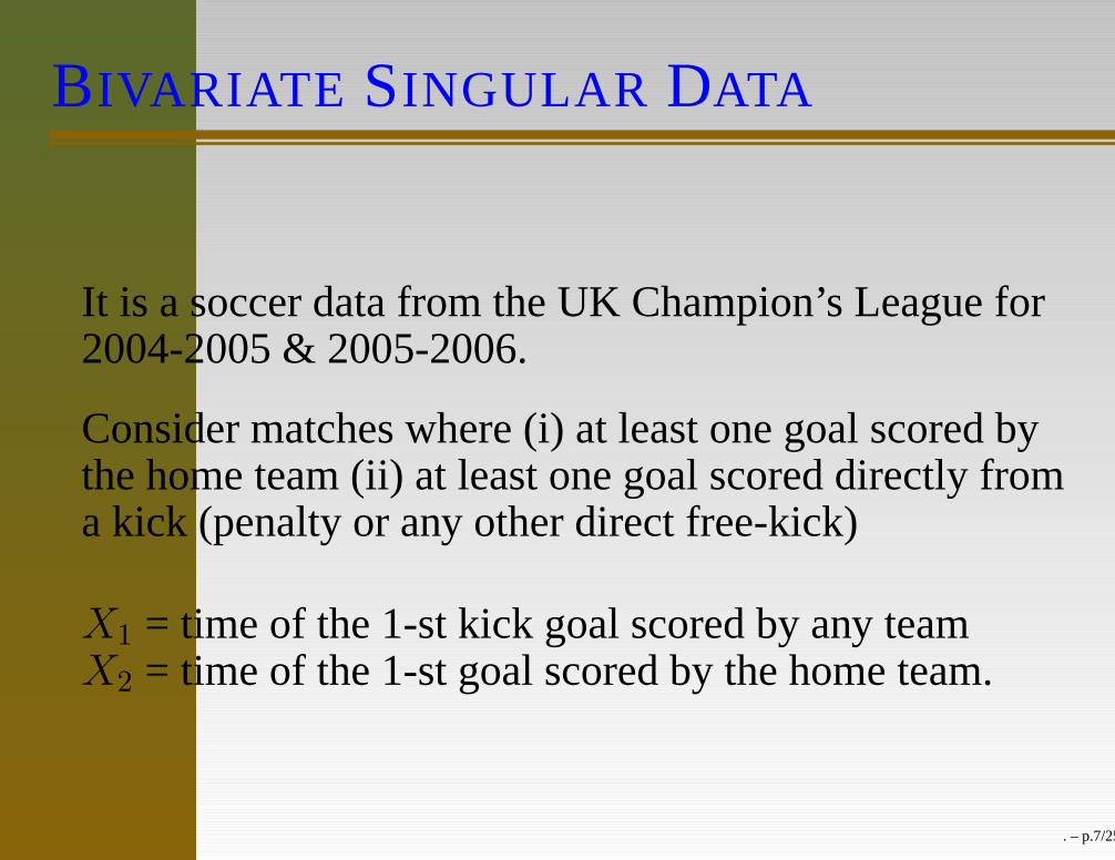
It is a soccer data from the UK Champion’s League for2004-2005 & 2005-2006.
Consider matches where (i) at least one goal scored bythe home team (ii) at least one goal scored directly froma kick (penalty or any other direct free-kick)
X1 = time of the 1-st kick goal scored by any teamX2 = time of the 1-st goal scored by the home team.
. – p.7/25
BIVARIATE SINGULAR DATA
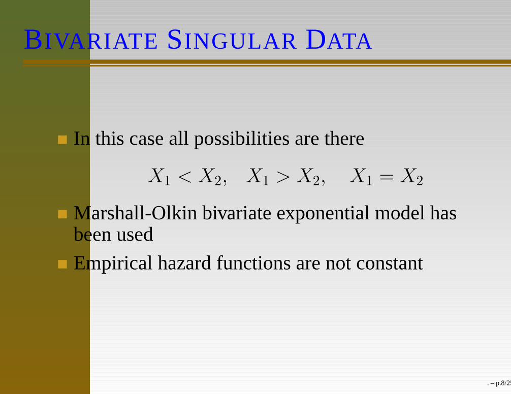
In this case all possibilities are there
X1 < X2, X1 > X2, X1 = X2
Marshall-Olkin bivariate exponential model hasbeen used
Empirical hazard functions are not constant
Empirical hazard function of X2 is an increasingfunction.
GE can be used quite effectively for fitting themarginals
. – p.8/25
BIVARIATE SINGULAR DATA
In this case all possibilities are there
X1 < X2, X1 > X2, X1 = X2
Marshall-Olkin bivariate exponential model hasbeen used
Empirical hazard functions are not constant
Empirical hazard function of X2 is an increasingfunction.
GE can be used quite effectively for fitting themarginals
. – p.8/25
BIVARIATE GE
Aim: We want a bivariate distribution whosemarginals are univariate GE distribution.
Idea: Came from the formulation of theMarshall-Olkin bivariate exponential model
Formulation:
U1 ∼ GE(α1, λ), U2 ∼ GE(α2, λ), U3 ∼ GE(α2, λ)
X1 = max{U1, U3}, X2 = max{U2, U3}
(X1, X2) ∼ BVGE(α1, α2, α3, λ)
. – p.9/25
INTERPRETATIONS
It may be observed as a
(a) Stress Model
(b) Maintenance Model
. – p.10/25
INTERPRETATIONS
It may be observed as a
(a) Stress Model
(b) Maintenance Model
. – p.10/25
INTERPRETATIONS
It may be observed as a
(a) Stress Model
(b) Maintenance Model
. – p.10/25
JOINT CDF
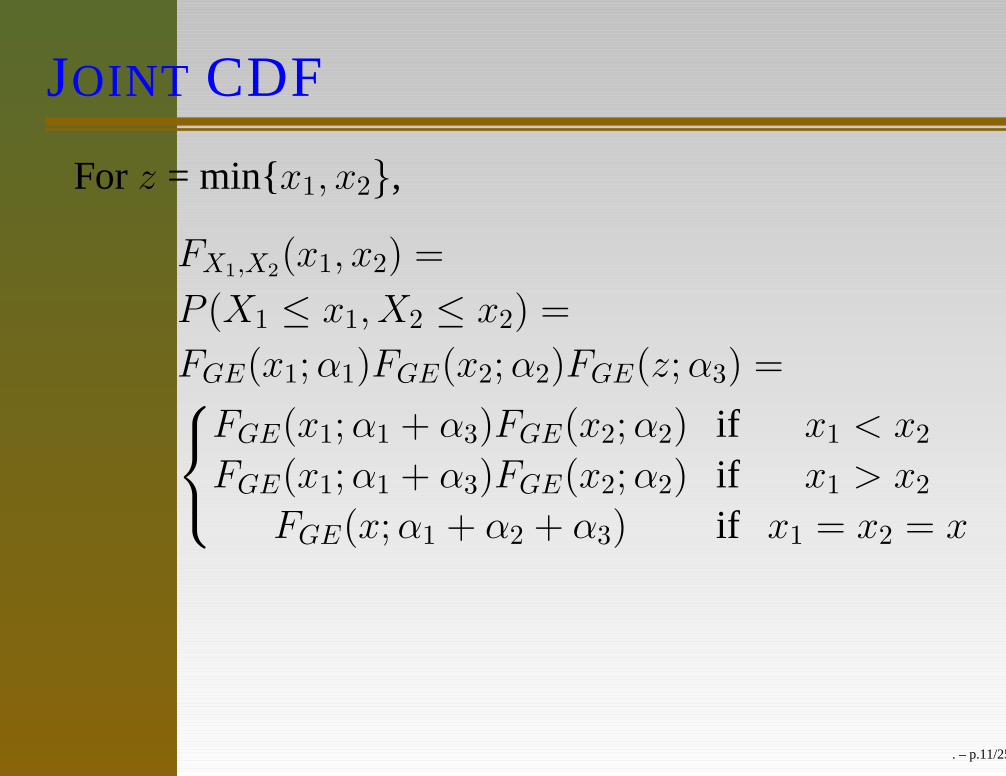
For z = min{x1, x2},
FX1,X2(x1, x2) =
P (X1 ≤ x1, X2 ≤ x2) =
FGE(x1;α1)FGE(x2;α2)FGE(z;α3) =
FGE(x1;α1 + α3)FGE(x2;α2) if x1 < x2
FGE(x1;α1 + α3)FGE(x2;α2) if x1 > x2
FGE(x;α1 + α2 + α3) if x1 = x2 = x
. – p.11/25
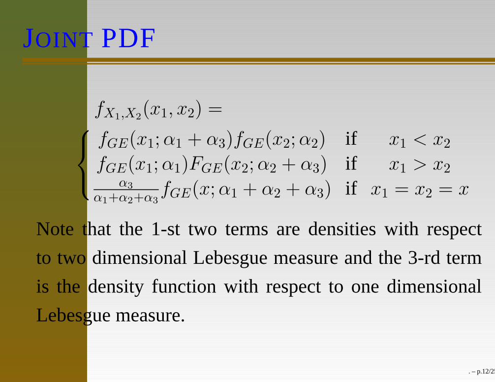
JOINT PDF
fX1,X2(x1, x2) =
fGE(x1;α1 + α3)fGE(x2;α2) if x1 < x2
fGE(x1;α1)FGE(x2;α2 + α3) if x1 > x2
α3
α1+α2+α3
fGE(x;α1 + α2 + α3) if x1 = x2 = x
Note that the 1-st two terms are densities with respect
to two dimensional Lebesgue measure and the 3-rd term
is the density function with respect to one dimensional
Lebesgue measure.
. – p.12/25
DECOMPOSITION OF CDF
The joint CDF can be written as
FX1,X2(x1, x2) = p Fa(x1, x2) + (1− p)Fs(x1, x2)
where
p =α1 + α2
α1 + α2 + α3
and for z = min{x1, x2}
Fs(x1, x2) = (1− e−z)α1+α2+α3.
Fa(x1, x2) can be obtained by subtraction.
. – p.13/25
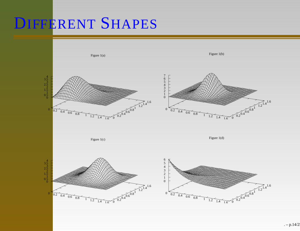
DIFFERENT SHAPES
Figure 1(a)
0 0.2 0.4 0.6 0.8 1 1.2 1.4 1.6 0 0.2
0.4 0.6
0.8 1
1.2 1.4
1.6 0
0.5 1
1.5 2
2.5 3
3.5 4
Figure 1(b)
0 0.2 0.4 0.6 0.8 1 1.2 1.4 1.6 0 0.2
0.4 0.6
0.8 1
1.2 1.4
1.6 0 1 2 3 4 5 6 7
Figure 1(c)
0 0.2 0.4 0.6 0.8 1 1.2 1.4 1.6 0 0.2
0.4 0.6
0.8 1
1.2 1.4
1.6 0
0.5 1
1.5 2
2.5 3
3.5 4
Figure 1(d)
0 0.2 0.4 0.6 0.8 1 1.2 1.4 1.6 0 0.2
0.4 0.6
0.8 1
1.2 1.4
1.6 0 1 2 3 4 5 6
. – p.14/25
MAXIMUM LIKELIHOOD ESTIMATES:
Without a proper estimation technique any modelmay not be useful in practice
Problems associated with the MLEs?
MLEs may not always exist.
Even if they exist they have to be obtained bysolving a four dimensional optimization problem.
. – p.15/25
MAXIMUM LIKELIHOOD ESTIMATES:
Without a proper estimation technique any modelmay not be useful in practice
Problems associated with the MLEs?
MLEs may not always exist.
Even if they exist they have to be obtained bysolving a four dimensional optimization problem.
. – p.15/25
MAXIMUM LIKELIHOOD ESTIMATES:
Without a proper estimation technique any modelmay not be useful in practice
Problems associated with the MLEs?
MLEs may not always exist.
Even if they exist they have to be obtained bysolving a four dimensional optimization problem.
. – p.15/25
MAXIMUM LIKELIHOOD ESTIMATES:
Without a proper estimation technique any modelmay not be useful in practice
Problems associated with the MLEs?
MLEs may not always exist.
Even if they exist they have to be obtained bysolving a four dimensional optimization problem.
. – p.15/25
MAXIMUM LIKELIHOOD ESTIMATES:
Without a proper estimation technique any modelmay not be useful in practice
Problems associated with the MLEs?
MLEs may not always exist.
Even if they exist they have to be obtained bysolving a four dimensional optimization problem.
. – p.15/25
EM ALGORITHM
We want to treat this problem as a missing valueproblem.
E-Step: Replace the missing observations by theirconditional expectation to form the pseudolikelihood function
M-Step: Maximize the pseudo likelihood function
. – p.16/25
EM ALGORITHM
We want to treat this problem as a missing valueproblem.
E-Step: Replace the missing observations by theirconditional expectation to form the pseudolikelihood function
M-Step: Maximize the pseudo likelihood function
. – p.16/25
EM ALGORITHM
We want to treat this problem as a missing valueproblem.
E-Step: Replace the missing observations by theirconditional expectation to form the pseudolikelihood function
M-Step: Maximize the pseudo likelihood function
. – p.16/25
EM ALGORITHM
We want to treat this problem as a missing valueproblem.
E-Step: Replace the missing observations by theirconditional expectation to form the pseudolikelihood function
M-Step: Maximize the pseudo likelihood function
. – p.16/25
EM ALGORITHM (CONT.)
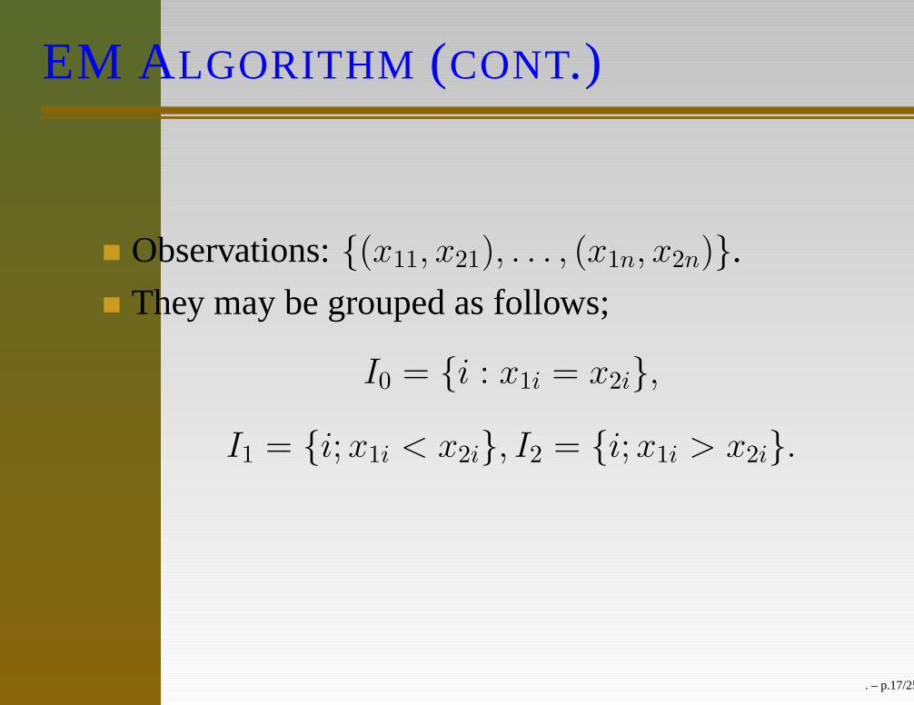
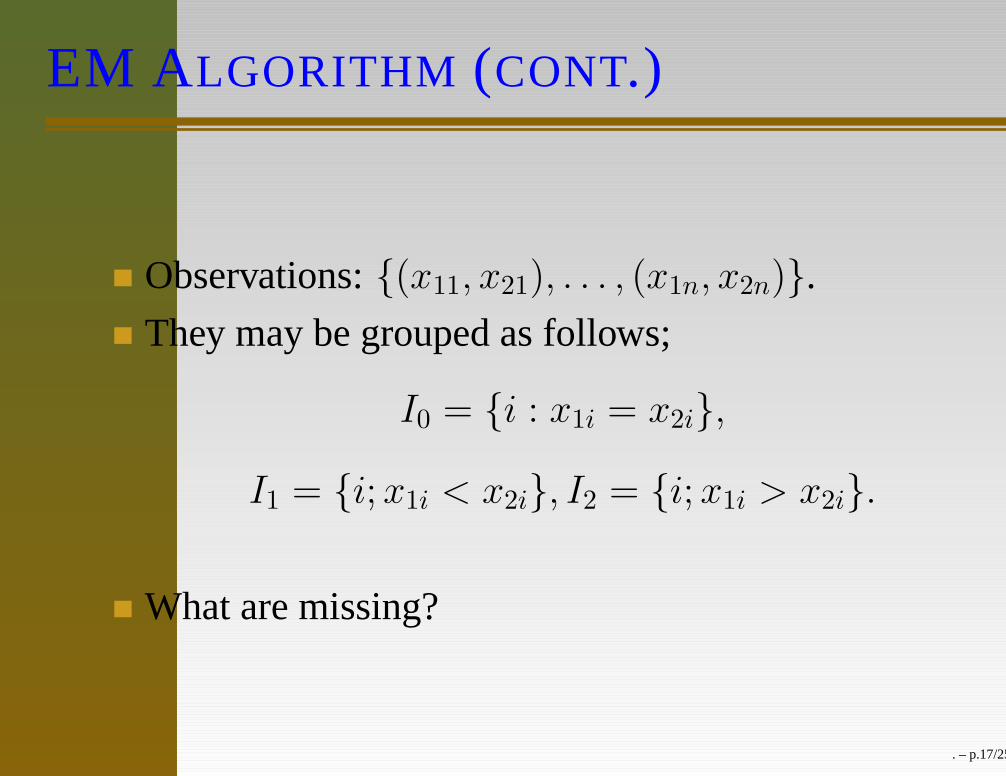
Observations: {(x11, x21), . . . , (x1n, x2n)}.
They may be grouped as follows;
I0 = {i : x1i = x2i},
I1 = {i;x1i < x2i}, I2 = {i;x1i > x2i}.
What are missing?
. – p.17/25
EM ALGORITHM (CONT.)
Observations: {(x11, x21), . . . , (x1n, x2n)}.
They may be grouped as follows;
I0 = {i : x1i = x2i},
I1 = {i;x1i < x2i}, I2 = {i;x1i > x2i}.
What are missing?
. – p.17/25
EM ALGORITHM (CONT.)
Observations: {(x11, x21), . . . , (x1n, x2n)}.
They may be grouped as follows;
I0 = {i : x1i = x2i},
I1 = {i;x1i < x2i}, I2 = {i;x1i > x2i}.
What are missing?
. – p.17/25
EM ALGORITHM (CONT.)
Observations: {(x11, x21), . . . , (x1n, x2n)}.
They may be grouped as follows;
I0 = {i : x1i = x2i},
I1 = {i;x1i < x2i}, I2 = {i;x1i > x2i}.
What are missing?
. – p.17/25
EM ALGORITHM (CONT.)
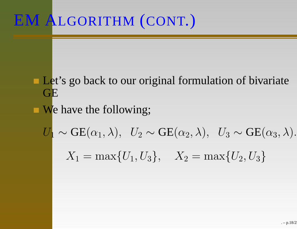
Let’s go back to our original formulation of bivariateGE
We have the following;
U1 ∼ GE(α1, λ), U2 ∼ GE(α2, λ), U3 ∼ GE(α3, λ).
X1 = max{U1, U3}, X2 = max{U2, U3}
. – p.18/25
EM ALGORITHM (CONT.)
Let’s go back to our original formulation of bivariateGE
We have the following;
U1 ∼ GE(α1, λ), U2 ∼ GE(α2, λ), U3 ∼ GE(α3, λ).
X1 = max{U1, U3}, X2 = max{U2, U3}
. – p.18/25
EM ALGORITHM (CONT.)
Let’s go back to our original formulation of bivariateGE
We have the following;
U1 ∼ GE(α1, λ), U2 ∼ GE(α2, λ), U3 ∼ GE(α3, λ).
X1 = max{U1, U3}, X2 = max{U2, U3}
. – p.18/25
EM ALGORITHM (CONT.)
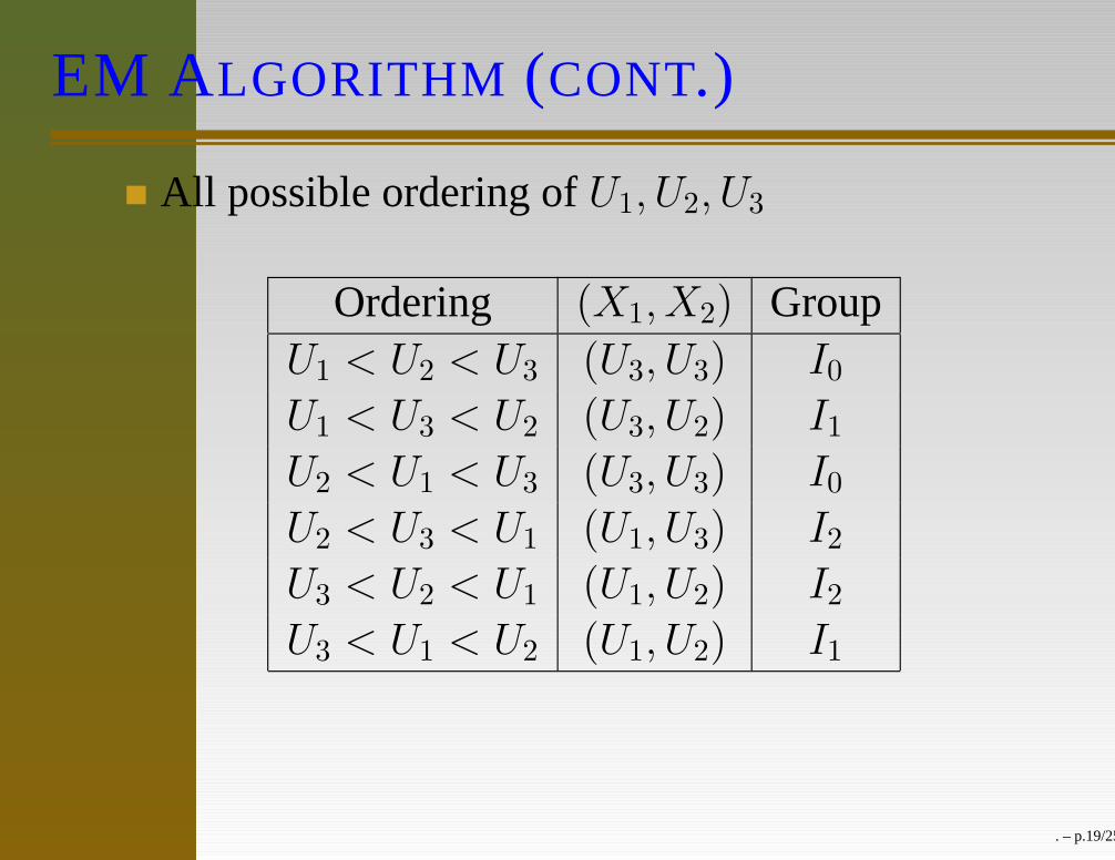
All possible ordering of U1, U2, U3
Ordering (X1, X2) GroupU1 < U2 < U3 (U3, U3) I0
U1 < U3 < U2 (U3, U2) I1
U2 < U1 < U3 (U3, U3) I0
U2 < U3 < U1 (U1, U3) I2
U3 < U2 < U1 (U1, U2) I2
U3 < U1 < U2 (U1, U2) I1
Suppose we know U1, U2, U3 along with X1, X2
. – p.19/25
EM ALGORITHM (CONT.)
All possible ordering of U1, U2, U3
Ordering (X1, X2) GroupU1 < U2 < U3 (U3, U3) I0
U1 < U3 < U2 (U3, U2) I1
U2 < U1 < U3 (U3, U3) I0
U2 < U3 < U1 (U1, U3) I2
U3 < U2 < U1 (U1, U2) I2
U3 < U1 < U2 (U1, U2) I1
Suppose we know U1, U2, U3 along with X1, X2
. – p.19/25
EM ALGORITHM (CONT.)
All possible ordering of U1, U2, U3
Ordering (X1, X2) GroupU1 < U2 < U3 (U3, U3) I0
U1 < U3 < U2 (U3, U2) I1
U2 < U1 < U3 (U3, U3) I0
U2 < U3 < U1 (U1, U3) I2
U3 < U2 < U1 (U1, U2) I2
U3 < U1 < U2 (U1, U2) I1
Suppose we know U1, U2, U3 along with X1, X2
. – p.19/25
EM ALGORITHM (CONT.)
The likelihood contribution of any observation from I0
fGE(x;α3, λ)FGE(x;α1 + α2, λ)
The likelihood contribution of any observation from I1
fGE(x1;α3, λ)fGE(x2;α2, λ)FGE(x1;α1, λ) or
fGE(x1;α1, λ)fGE(x2;α2, λ)FGE(x1;α3, λ).
The likelihood contribution of any observation from I2
Therefore in this case the complete observation is of thefollowing type
(X1, X2,Λ1,Λ2)
Here Λ1 and Λ2 are as follows;
Λ1 =
{
1 if X1 = U1
3 if X1 = U3
Λ2 =
{
2 if X2 = U2
3 if X2 = U3
. – p.21/25
EM ALGORITHM (CONT.); E-STEP
Therefore for the Group I0 both Λ1 and Λ2 are known.
Λ1 = Λ2 = 3
For Group I1 Λ2 is known and Λ1 is unknown.
Λ1 = 1 or 3, Λ2 = 2
For Group I2 Λ1 is known and Λ2 is unknown.
Λ1 = 1, Λ2 = 2 or 3.
Moreover
P (Λ1 = 1|I1) =α1
α1 + α3
, P (Λ2 = 2|I2) =α2
α2 + α3
,
. – p.22/25
EM ALGORITHM (CONT.); M-STEP
With the above information the pseudo log-likelihoodfunction can be written. For M-step we need to maximizethe pseudo log-likelihood function with respect to theunknown parameters. The pseudo log-likelihoodfunction can be written as a profile log-likelihoodfunction of λ only and the maximization can be carriedout as a one dimensional optimization method.
. – p.23/25
GENERALIZATIONS
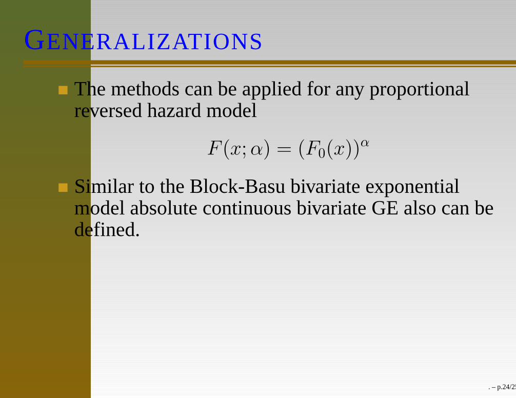
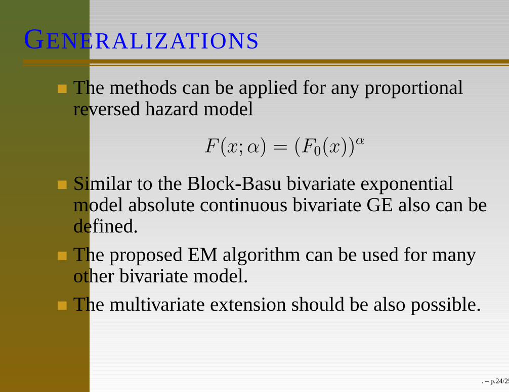
The methods can be applied for any proportionalreversed hazard model
F (x;α) = (F0(x))α
Similar to the Block-Basu bivariate exponentialmodel absolute continuous bivariate GE also can bedefined.
The proposed EM algorithm can be used for manyother bivariate model.
The multivariate extension should be also possible.
Bayesian inference
. – p.24/25
GENERALIZATIONS
The methods can be applied for any proportionalreversed hazard model
F (x;α) = (F0(x))α
Similar to the Block-Basu bivariate exponentialmodel absolute continuous bivariate GE also can bedefined.
The proposed EM algorithm can be used for manyother bivariate model.
The multivariate extension should be also possible.