Macalester College Macalester College DigitalCommons@Macalester College DigitalCommons@Macalester College Economics Honors Projects Economics Department Summer 5-1-2021 Demand Shock along the Supply Chain: The Bullwhip Effect of Demand Shock along the Supply Chain: The Bullwhip Effect of Covid-19 in Chinese Exports Covid-19 in Chinese Exports Kaichong Zhang Macalester College, [email protected]Follow this and additional works at: https://digitalcommons.macalester.edu/economics_honors_projects Part of the Economics Commons Recommended Citation Recommended Citation Zhang, Kaichong, "Demand Shock along the Supply Chain: The Bullwhip Effect of Covid-19 in Chinese Exports" (2021). Economics Honors Projects. 108. https://digitalcommons.macalester.edu/economics_honors_projects/108 This Honors Project - Open Access is brought to you for free and open access by the Economics Department at DigitalCommons@Macalester College. It has been accepted for inclusion in Economics Honors Projects by an authorized administrator of DigitalCommons@Macalester College. For more information, please contact [email protected].
Transcript
Macalester College Macalester College
DigitalCommons@Macalester College DigitalCommons@Macalester College
Economics Honors Projects Economics Department
Summer 5-1-2021
Demand Shock along the Supply Chain: The Bullwhip Effect of Demand Shock along the Supply Chain: The Bullwhip Effect of
Covid-19 in Chinese Exports Covid-19 in Chinese Exports
Follow this and additional works at: https://digitalcommons.macalester.edu/economics_honors_projects
Part of the Economics Commons
Recommended Citation Recommended Citation Zhang, Kaichong, "Demand Shock along the Supply Chain: The Bullwhip Effect of Covid-19 in Chinese Exports" (2021). Economics Honors Projects. 108. https://digitalcommons.macalester.edu/economics_honors_projects/108
This Honors Project - Open Access is brought to you for free and open access by the Economics Department at DigitalCommons@Macalester College. It has been accepted for inclusion in Economics Honors Projects by an authorized administrator of DigitalCommons@Macalester College. For more information, please contact [email protected].
I would like to express my special gratitude to my advisors, Professor Felix L Friedt and Professor AmyDamon, my Economics Honors Thesis committee members, Professor Liang Ding and Professor DavidShuman, as well as my Honors Thesis classmates who gave me excellent supports and illuminatingcomments to my research project.
THE BULLWHIP EFFECT OF COVID-19 IN CHINESE EXPORTS 2
Abstract
This study investigates the bullwhip effect of Covid-19 on global supply chains from the
Chinese perspective. The bullwhip effect refers to the amplification of demand shock along
the supply chain, and my baseline estimates show that a 1% increase in foreign new cases
(a proxy for foreign demand shock) reduces exports of downstream products and that of
upstream industries by 2.1% and 4.5% respectively. The estimates also suggest that
whether industries are concentrated or not generates ambiguous effects on exports that
vary from different empirical specifications. In addition, a heterogeneity analysis suggests
that the bullwhip effect is stronger in regional supply chains among geographically
proximate countries and countries that are closely connected in terms of the trade volume.
Furthermore, a dynamic analysis shows that the outbreak of Covid-19 in foreign countries
causes a lagged import substitution towards Chinese products that reverses the initially
negative demand shock. Unlike the initial adverse effect, I find that the lagged import
substitution does not amplify along the supply chain, but mostly affects downstream
industries.
Keywords: Global Pandemic, Covid-19, International Trade, Bullwhip Effect, Supply
Chains, Demand Shock
THE BULLWHIP EFFECT OF COVID-19 IN CHINESE EXPORTS 3
1 Introduction
The Covid-19 crisis began in December 2019 and has already infected more than 115
million people and caused more than 2 million deaths around the world. The public health
crisis was accompanied by the global economic recession and the pandemic shock is as
contagious economically as it is medically in the increasingly interconnected world
(R. Baldwin, di Mauro, & Tomiura, 2020). A report from World Trade Organization
predicted that the global trade in merchandise will decrease 9.2% in 2020 and the trade
volume will remain below the pre-crisis level in 2021 (World Trade Organization, 2020).
More importantly, the major trading nations, including US, China, Japan, Germany,
Britain, France, and Italy, that account for 60% of world GDP, 65% of world
manufacturing, and 41% of global manufacturing exports, are also the hardest-hit nations
(R. Baldwin et al., 2020). As a result of the contagion of international production
networks, the Covid shock leads to drastic welfare losses. China, for example, is expected
to experience a welfare loss of about 30%, and such loss will spill over around the world
through Global Value Chains (GVCs) (Eppinger, Felbermayr, Krebs, & Kukharskyy, 2020;
Friedt & Zhang, 2020).
Many scholars explore the general mechanism of the Covid shock from either the
demand side (the drop in aggregate demand and the "wait-and-see" purchase/investment
delays) or the supply side (factory closures and supply-chain contagions) (see Balleer, Link,
Menkhoff, and Zorn (2020); Bekaert, Engstrom, and Ermolov (2020); Hyun, Kim, and Shin
(2020); Meier and Pinto (2020)). However, while previous works have shown that sudden
shocks in demand can create a ‘bullwhip effect’ along the supply chain (Altomonte,
Di Mauro, Ottaviano, Rungi, & Vicard, 2012; Zavacka, 2012), none of the Covid studies
focus on this particular area.3 This effect refers to the amplification of order volatility
along the supply chain (Wang & Disney, 2016). It has been well studied by Altomonte et
3 Although the bullwhip effect is briefly mentioned by some scholars like R. Baldwin et al. (2020) andPatrinley et al. (2020), they only suggest the possibility that the effect exists and can negatively affect themanufacturing sectors without delving into the details of the bullwhip effect.
THE BULLWHIP EFFECT OF COVID-19 IN CHINESE EXPORTS 4
al. (2012) and Zavacka (2012) in the context of the demand-driven 2008 Global Trade
Collapse (GTC). They demonstrate the impact of the bullwhip effect along the supply
chains and argue that the effect was mainly caused by the adjustment of production and
inventory to new expectation. More specifically, the volatility of sales would increase from
downstream to upstream industries, making upstream producers more likely to drop out of
trade shortly after the GTC.
In this paper, I analyze the bullwhip effect of Covid-19 on global supply chains from
the Chinese perspective. I first develop a simple theoretical framework to motivate my
empirical analysis. The model demonstrates the mechanisms underlying the theorized
bullwhip effect and explores how this effect is shaped by the degree of industry
concentration. My primary empirical model uses Chinese new cases as a proxy for the
Chinese domestic supply shock and uses foreign new cases to measure the foreign demand
shock. The initial analysis provides baseline estimates showing that upstream industries
tend to suffer more from an amplified demand shock compared to downstream ones.
Moreover, concentrated industries tend to experience a weaker demand shock compared to
non-concentrated ones. Statistically, a 1% increase in foreign new cases leads to 2.6%
reduction in exports of downstream and non-concentrated industries, 4.7% reduction in
exports if the industries are upstream, and only 0.2% reduction in exports if the industries
are concentrated. The estimates are significant at 0.01 level and are robust against
different fixed effects specifications, alternative measurements of the severity of the
pandemic, and various sample restrictions.
Building on these baseline results, I conduct heterogeneity analyses that test the
sensitivity of the estimated bullwhip effect along several dimensions. Restricting the
sample to Asian countries, I find that the bullwhip effect is stronger among the regional
supply chain network. Further restricting the sample to include only the top 30 Chinese
trading partners according to trade data in 2019, I find that the demand shock upstream
industries suffer is even stronger. Specifically, the estimates reveal that 1% increase in
THE BULLWHIP EFFECT OF COVID-19 IN CHINESE EXPORTS 5
foreign new cases amplifies the reduction of upstream exports from 4.7% to 5.0% for Asian
supply chains and to 5.7% for supply chains among Chinese major trading partners. These
regression results suggest that the bullwhip effect is more prominent in supply chains in
which countries are geographically proximate and are economically closely connected.
Lastly, as the conceptual model suggests that the bullwhip effect is dynamic in nature
and upstream industries tend to suffer from a delayed instead of immediate demand shock
that transmits along the supply chains, I examine the time lagged bullwhip effect by
exploring the nuance of the demand shock month by month after the outbreak of Covid-19.
The analysis, however, raises two important issues that are at odds with the stylized
model: (1) the demand shock hits upstream and downstream industries at the same time
within the first month after the outbreak of Covid-19; (2) while the lagged effects
demonstrate a quick recovery in exports of Chinese downstream products and a reversal of
the initial adverse demand shock, exports of upstream products are slower to recover and
do not experience an amplified lagged positive demand shock.
The first deviation can be explained by the frequency of the observed trade data.
Although the theorized bullwhip effect suggests the delayed demand shock on upstream
industries, it does not specify the lag length. Given the advanced communication
technology nowadays, it is possible that the amplified demand shock hits the most
upstream industry within a month of the initial shock. In this case, such short
postponement is unobservable in monthly trade data.
The second deviation is harder to reconcile with the theorized bullwhip effect. One
potential explanation is that the lagged positive demand shock on exports of downstream
industries represents the significant import substitution from heavily affected foreign
countries, where factory closures stagnate the foreign production process and foreign raw
material imports from Chinese upstream industries. In this case, foreign consumers’
demand for final goods can only be fulfilled by Chinese downstream producers. As a result,
the positive demand shock that hits downstream industries does not amplify along the
THE BULLWHIP EFFECT OF COVID-19 IN CHINESE EXPORTS 6
proportion of the supply chains that involve foreign producers, which remain shut down,
and leads to weak recovery of upstream exports 2 to 5 months after the initial outbreak.
This study contributes to several strands of the economic literature. My findings offer
new insights on the pandemic effects on international trade and therefore advance the
rapidly growing research on Covid-19. Bonadio, Huo, Levchenko, and Pandalai-Nayar
(2020) and Antras, Redding, and Rossi-Hansberg (2020), for example, show that the
lockdown of the major trading nations and the disruption of global trade can explain one
third of the downturn of the global economy. Theoretically, the lockdown affects
international trade through three channels: the demand shock, the supply shock, and the
THE BULLWHIP EFFECT OF COVID-19 IN CHINESE EXPORTS 7
attitude strongly hurt the "postponeable goods4" that comprised a major portion of the
global trade (R. Baldwin & Taglioni, 2009). Firms engaged in global manufacturing in
2008 had difficulty managing their inventory and therefore were at risk of the bullwhip
effect (Altomonte et al., 2012; Leckcivilize, 2012). But both SARS and GTC are still
different from the current Covid-19 crisis as there was no severe and widespread supply
chain disruptions and GVC contagions in 2003 and 2008 and the impacted area of the
SARS did not cover the major trading nations, like the United States and the European
Union (Fernandes & Tang, 2020).
The rest of the paper is structured as follows. Section 2 presents a theoretical model
building on the works by Altomonte et al. (2012) and Zavacka (2012). Section 3 introduces
the data and discusses the relevant summary statistics. Section 4 provides the baseline
estimates with robustness checks and geographic heterogeneity analysis. I also incorporate
a dynamic analysis to explore the nuance of the lagged bullwhip effect and make a
comparison between the theory and the empirical results. Section 6 concludes the paper
and sheds lights upon the policy implications and the directions of future studies.
2 Theoretical Model
The bullwhip effect refers to the amplification of demand shock along the supply
chain. The following theoretical model demonstrates two key features of the bullwhip effect.
First, the more upstream the producers are, the greater the demand shock they suffer. The
demand shock that hits the most downstream producers amplifies as it transmits along the
supply chain to the most upstream ones. Second, diversification of output (or downstream
industries) matters. Depending on the relationships among downstream products,
upstream producers who have various downstream recipients can either reduce or further
exacerbate their order volatility. The following model is built on the studies by Altomonte
et al. (2012) and Zavacka (2012) who analyze the bullwhip effect resulting from 2008 GTC.
4 This phrase is introduced by Richard Baldwin and Daria Taglioni and refers to products like new andupdated equipment that are durable and that consumers don’t have to buy immediately.
THE BULLWHIP EFFECT OF COVID-19 IN CHINESE EXPORTS 8
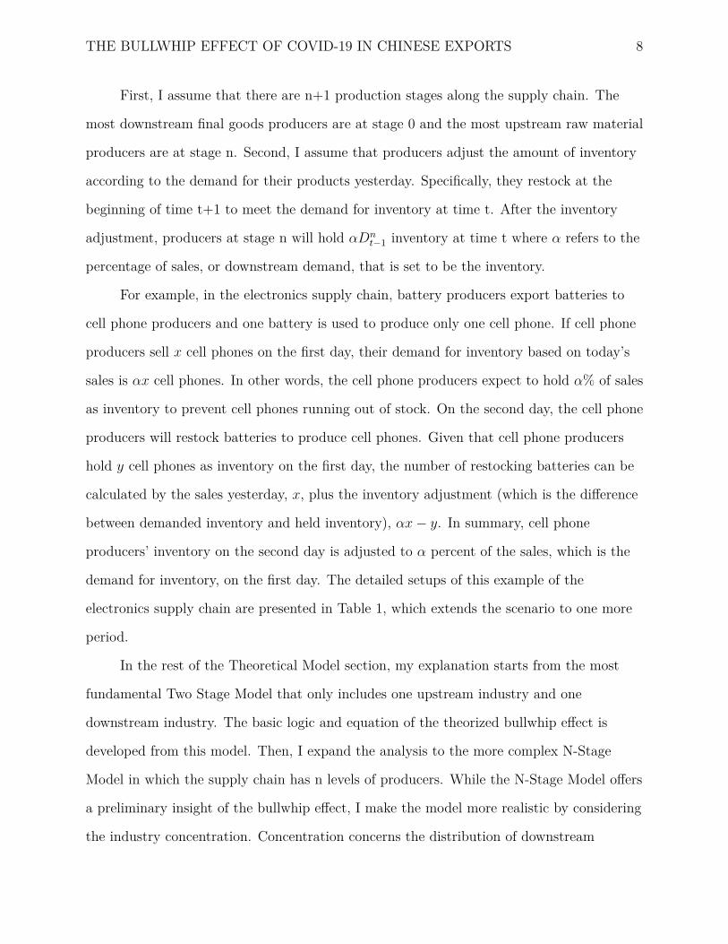
First, I assume that there are n+1 production stages along the supply chain. The
most downstream final goods producers are at stage 0 and the most upstream raw material
producers are at stage n. Second, I assume that producers adjust the amount of inventory
according to the demand for their products yesterday. Specifically, they restock at the
beginning of time t+1 to meet the demand for inventory at time t. After the inventory
adjustment, producers at stage n will hold αDnt−1 inventory at time t where α refers to the
percentage of sales, or downstream demand, that is set to be the inventory.
For example, in the electronics supply chain, battery producers export batteries to
cell phone producers and one battery is used to produce only one cell phone. If cell phone
producers sell x cell phones on the first day, their demand for inventory based on today’s
sales is αx cell phones. In other words, the cell phone producers expect to hold α% of sales
as inventory to prevent cell phones running out of stock. On the second day, the cell phone
producers will restock batteries to produce cell phones. Given that cell phone producers
hold y cell phones as inventory on the first day, the number of restocking batteries can be
calculated by the sales yesterday, x, plus the inventory adjustment (which is the difference
between demanded inventory and held inventory), αx− y. In summary, cell phone
producers’ inventory on the second day is adjusted to α percent of the sales, which is the
demand for inventory, on the first day. The detailed setups of this example of the
electronics supply chain are presented in Table 1, which extends the scenario to one more
period.
In the rest of the Theoretical Model section, my explanation starts from the most
fundamental Two Stage Model that only includes one upstream industry and one
downstream industry. The basic logic and equation of the theorized bullwhip effect is
developed from this model. Then, I expand the analysis to the more complex N-Stage
Model in which the supply chain has n levels of producers. While the N-Stage Model offers
a preliminary insight of the bullwhip effect, I make the model more realistic by considering
the industry concentration. Concentration concerns the distribution of downstream
THE BULLWHIP EFFECT OF COVID-19 IN CHINESE EXPORTS 9
recipients; if an industry is highly concentrated, it sells its products to only one
downstream industry; if an industry is not concentrated, it exports its products to many
downstream industries.
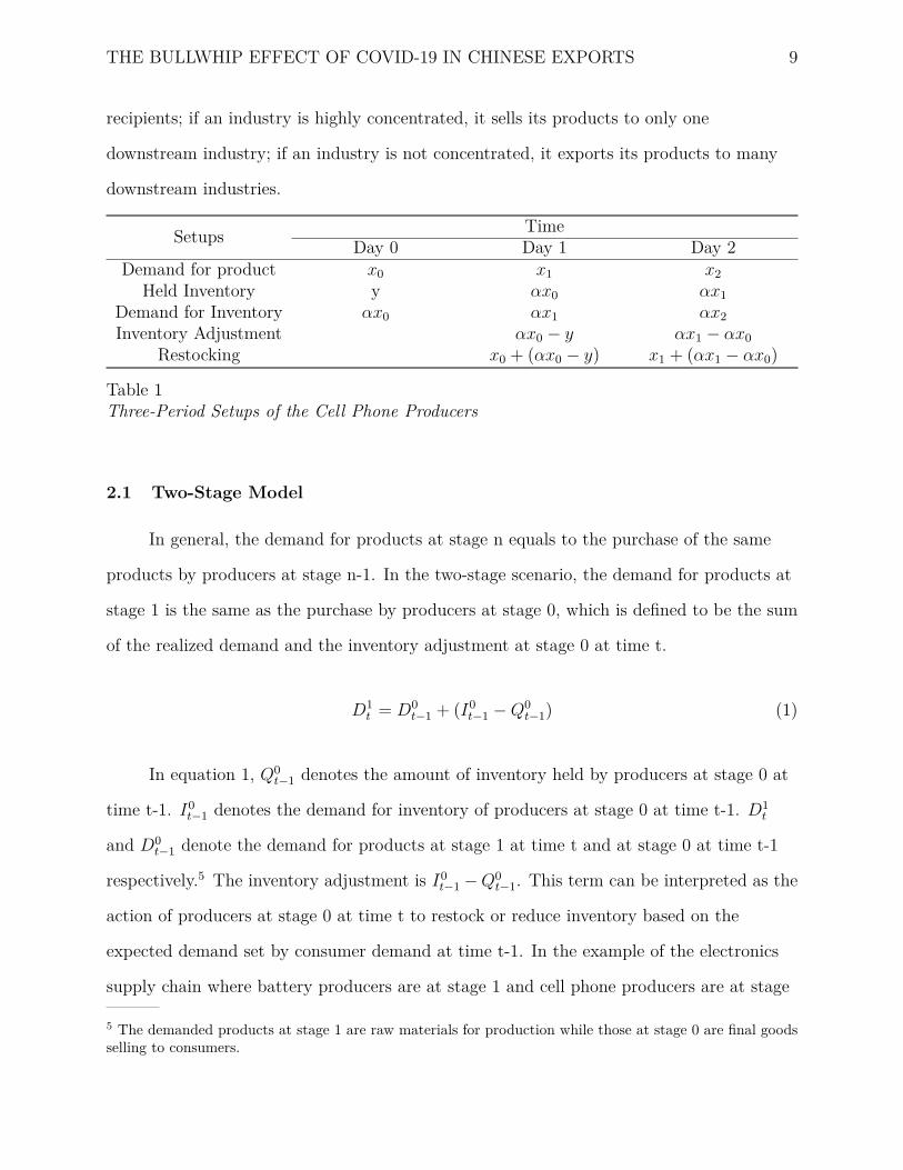
Setups TimeDay 0 Day 1 Day 2
Demand for product x0 x1 x2Held Inventory y αx0 αx1
Demand for Inventory αx0 αx1 αx2Inventory Adjustment αx0 − y αx1 − αx0
Restocking x0 + (αx0 − y) x1 + (αx1 − αx0)
Table 1Three-Period Setups of the Cell Phone Producers
2.1 Two-Stage Model
In general, the demand for products at stage n equals to the purchase of the same
products by producers at stage n-1. In the two-stage scenario, the demand for products at
stage 1 is the same as the purchase by producers at stage 0, which is defined to be the sum
of the realized demand and the inventory adjustment at stage 0 at time t.
D1t = D0
t−1 + (I0t−1 −Q0
t−1) (1)
In equation 1, Q0t−1 denotes the amount of inventory held by producers at stage 0 at
time t-1. I0t−1 denotes the demand for inventory of producers at stage 0 at time t-1. D1
t
and D0t−1 denote the demand for products at stage 1 at time t and at stage 0 at time t-1
respectively.5 The inventory adjustment is I0t−1 −Q0
t−1. This term can be interpreted as the
action of producers at stage 0 at time t to restock or reduce inventory based on the
expected demand set by consumer demand at time t-1. In the example of the electronics
supply chain where battery producers are at stage 1 and cell phone producers are at stage
5 The demanded products at stage 1 are raw materials for production while those at stage 0 are final goodsselling to consumers.
THE BULLWHIP EFFECT OF COVID-19 IN CHINESE EXPORTS 10
0, if nothing happens, cell phone producers will demand the same amount of inventory and
I0t−1 −Q0
t−1 = 0 (there is no inventory adjustment). If cell phone producers have more
inventory than they needed, that is if I0t−1 < Q0
t−1, they will decrease their order for
products at stage 1. But if cell phone producers demand more inventory as their products
are popular in the market, that is if I0t−1 > Q0
t−1, they will increase their order for products
at stage 1.
Based on the second assumption that producers will set their inventory to α percent
of the sales, the demand for inventory can be written as I0t−1 = αD0
t−1. Building on the
same assumption that the demand for inventory today is equal to the amount of inventory
tomorrow, the inventory at time t-1 equals to the demand for inventory at time t-2
(Q0t−1 = I0
t−2 = αD0t−2. Then, we can rewrite equation 1 to:
D1t = D0
t−1 + (I0t−1 −Q0
t−1)
= D0t−1 + αD0
t−1 − αD0t−2
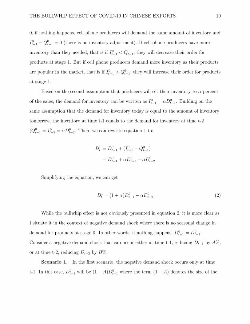
Simplifying the equation, we can get
D1t = (1 + α)D0
t−1 − αD0t−2 (2)
While the bullwhip effect is not obviously presented in equation 2, it is more clear as
I situate it in the context of negative demand shock where there is no seasonal change in
demand for products at stage 0. In other words, if nothing happens, D0t−1 = D0
t−2.
Consider a negative demand shock that can occur either at time t-1, reducing Dt−1 by A%,
or at time t-2, reducing Dt−2 by B%.
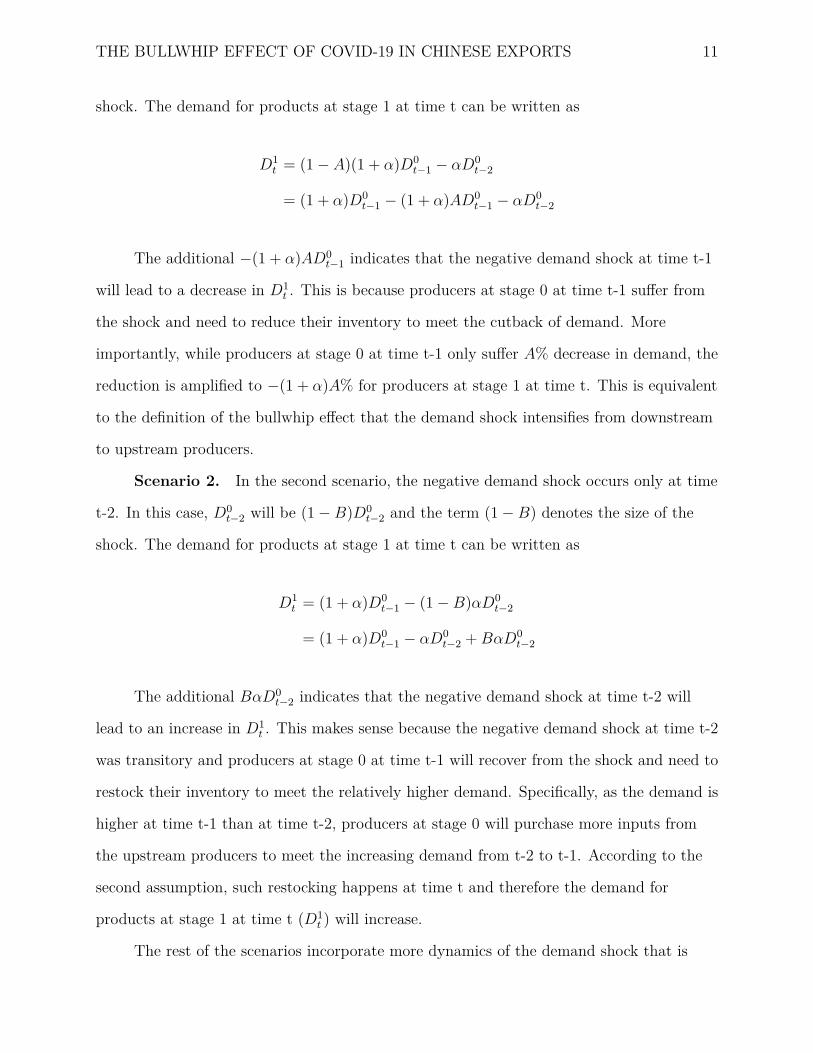
Scenario 1. In the first scenario, the negative demand shock occurs only at time
t-1. In this case, D0t−1 will be (1 − A)D0
t−1 where the term (1 − A) denotes the size of the
THE BULLWHIP EFFECT OF COVID-19 IN CHINESE EXPORTS 11
shock. The demand for products at stage 1 at time t can be written as
D1t = (1 − A)(1 + α)D0
t−1 − αD0t−2
= (1 + α)D0t−1 − (1 + α)AD0
t−1 − αD0t−2
The additional −(1 + α)AD0t−1 indicates that the negative demand shock at time t-1
will lead to a decrease in D1t . This is because producers at stage 0 at time t-1 suffer from
the shock and need to reduce their inventory to meet the cutback of demand. More
importantly, while producers at stage 0 at time t-1 only suffer A% decrease in demand, the
reduction is amplified to −(1 + α)A% for producers at stage 1 at time t. This is equivalent
to the definition of the bullwhip effect that the demand shock intensifies from downstream
to upstream producers.
Scenario 2. In the second scenario, the negative demand shock occurs only at time
t-2. In this case, D0t−2 will be (1 −B)D0
t−2 and the term (1 −B) denotes the size of the
shock. The demand for products at stage 1 at time t can be written as
D1t = (1 + α)D0
t−1 − (1 −B)αD0t−2
= (1 + α)D0t−1 − αD0
t−2 +BαD0t−2
The additional BαD0t−2 indicates that the negative demand shock at time t-2 will
lead to an increase in D1t . This makes sense because the negative demand shock at time t-2
was transitory and producers at stage 0 at time t-1 will recover from the shock and need to
restock their inventory to meet the relatively higher demand. Specifically, as the demand is
higher at time t-1 than at time t-2, producers at stage 0 will purchase more inputs from
the upstream producers to meet the increasing demand from t-2 to t-1. According to the
second assumption, such restocking happens at time t and therefore the demand for
products at stage 1 at time t (D1t ) will increase.
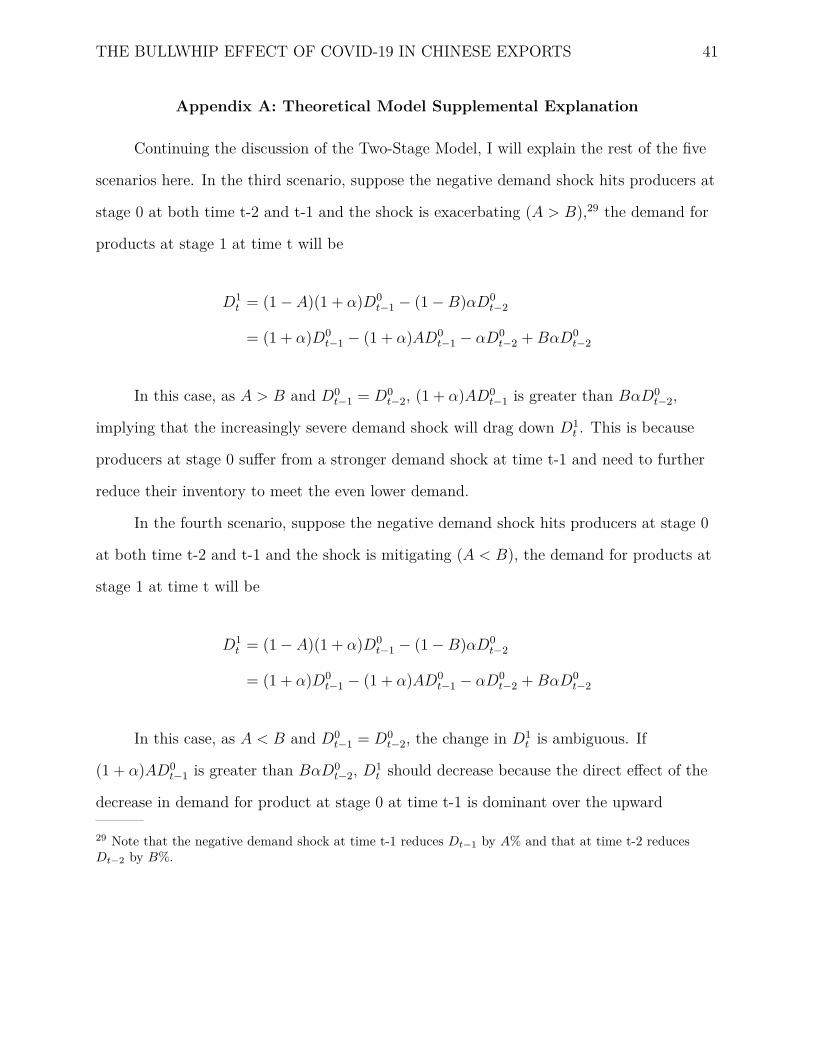
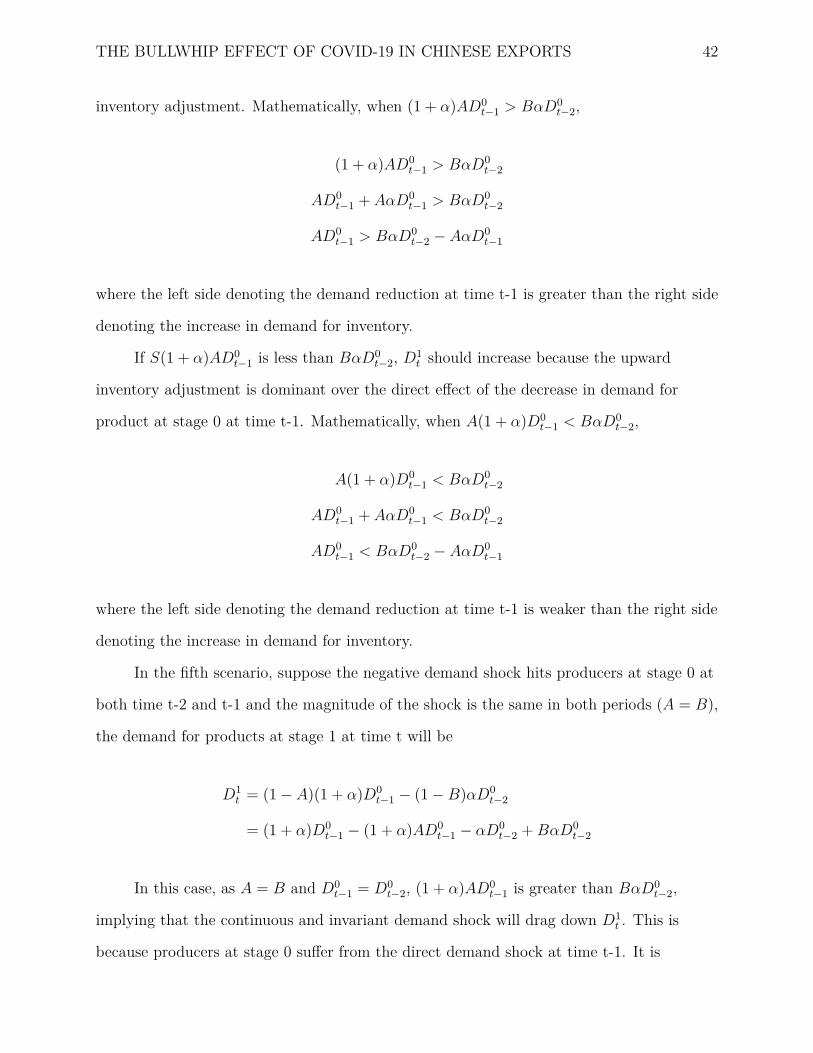
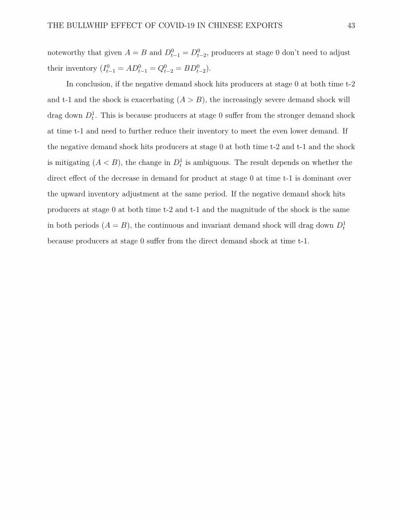
The rest of the scenarios incorporate more dynamics of the demand shock that is
THE BULLWHIP EFFECT OF COVID-19 IN CHINESE EXPORTS 12
persistent at both time t-1 and t-2. Specifically, the shock can be exacerbating, mitigating,
and stationary6 in both periods. The detailed mathematical proofs are shown in the
Appendix A. In short, in the context of negative demand shock, equation 2 can effectively
demonstrate the bullwhip effect.
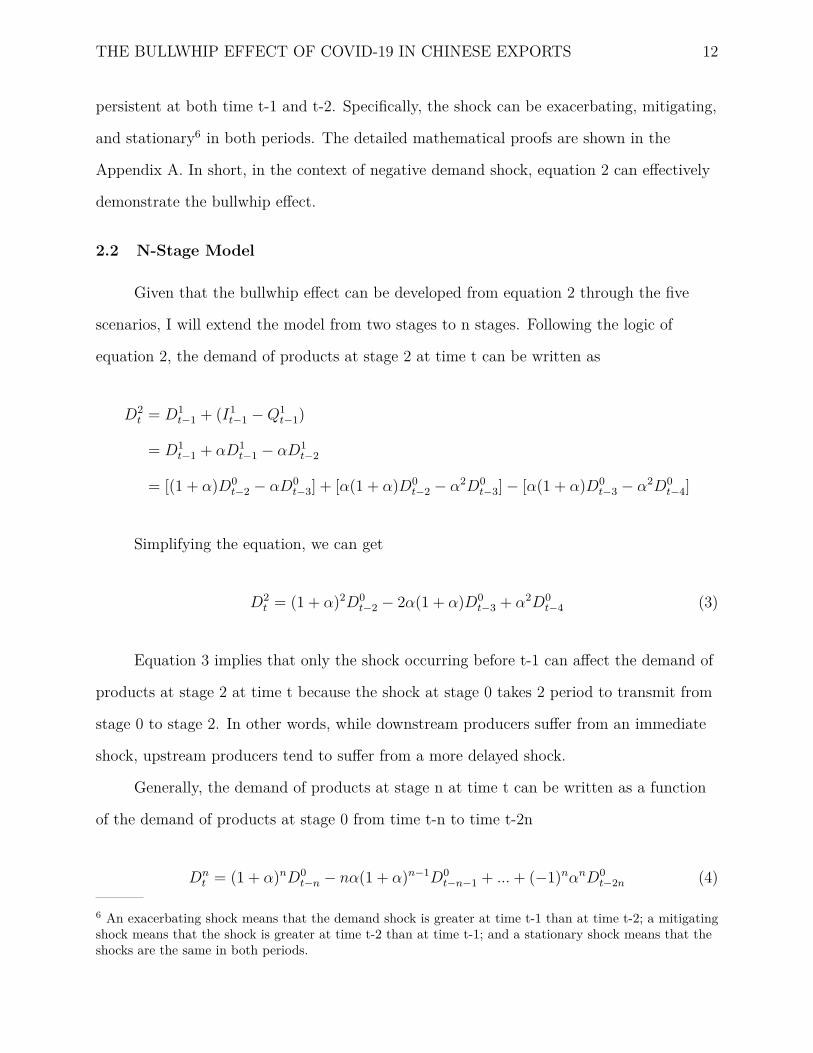
2.2 N-Stage Model
Given that the bullwhip effect can be developed from equation 2 through the five
scenarios, I will extend the model from two stages to n stages. Following the logic of
equation 2, the demand of products at stage 2 at time t can be written as
D2t = D1
t−1 + (I1t−1 −Q1
t−1)
= D1t−1 + αD1
t−1 − αD1t−2
= [(1 + α)D0t−2 − αD0
t−3] + [α(1 + α)D0t−2 − α2D0
t−3] − [α(1 + α)D0t−3 − α2D0
t−4]
Simplifying the equation, we can get
D2t = (1 + α)2D0
t−2 − 2α(1 + α)D0t−3 + α2D0
t−4 (3)
Equation 3 implies that only the shock occurring before t-1 can affect the demand of
products at stage 2 at time t because the shock at stage 0 takes 2 period to transmit from
stage 0 to stage 2. In other words, while downstream producers suffer from an immediate
shock, upstream producers tend to suffer from a more delayed shock.
Generally, the demand of products at stage n at time t can be written as a function
of the demand of products at stage 0 from time t-n to time t-2n
Dnt = (1 + α)nD0
t−n − nα(1 + α)n−1D0t−n−1 + ...+ (−1)nαnD0
t−2n (4)
6 An exacerbating shock means that the demand shock is greater at time t-1 than at time t-2; a mitigatingshock means that the shock is greater at time t-2 than at time t-1; and a stationary shock means that theshocks are the same in both periods.
THE BULLWHIP EFFECT OF COVID-19 IN CHINESE EXPORTS 13
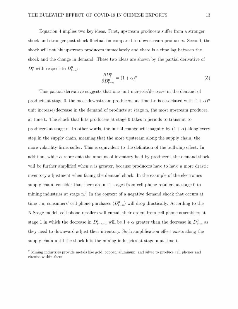
Equation 4 implies two key ideas. First, upstream producers suffer from a stronger
shock and stronger post-shock fluctuation compared to downstream producers. Second, the
shock will not hit upstream producers immediately and there is a time lag between the
shock and the change in demand. These two ideas are shown by the partial derivative of
Dnt with respect to D0
t−n:∂Dn
t
∂D0t−n
= (1 + α)n (5)
This partial derivative suggests that one unit increase/decrease in the demand of
products at stage 0, the most downstream producers, at time t-n is associated with (1 +α)n
unit increase/decrease in the demand of products at stage n, the most upstream producer,
at time t. The shock that hits producers at stage 0 takes n periods to transmit to
producers at stage n. In other words, the initial change will magnify by (1 + α) along every
step in the supply chain, meaning that the more upstream along the supply chain, the
more volatility firms suffer. This is equivalent to the definition of the bullwhip effect. In
addition, while α represents the amount of inventory held by producers, the demand shock
will be further amplified when α is greater, because producers have to have a more drastic
inventory adjustment when facing the demand shock. In the example of the electronics
supply chain, consider that there are n+1 stages from cell phone retailers at stage 0 to
mining industries at stage n.7 In the context of a negative demand shock that occurs at
time t-n, consumers’ cell phone purchases (D0t−n) will drop drastically. According to the
N-Stage model, cell phone retailers will curtail their orders from cell phone assemblers at
stage 1 in which the decrease in D1t−n+1 will be 1 + α greater than the decrease in D0
t−n as
they need to downward adjust their inventory. Such amplification effect exists along the
supply chain until the shock hits the mining industries at stage n at time t.
7 Mining industries provide metals like gold, copper, aluminum, and silver to produce cell phones andcircuits within them.
THE BULLWHIP EFFECT OF COVID-19 IN CHINESE EXPORTS 14
2.3 N-Stage Model with Concentration
While equation 5 explains the bullwhip effect in terms of the relationship between the
upstreamness and the demand volatility, it does not fit well to the reality as it assumes
that the supply chain does not bifurcate and each stage has a one to one relationship with
its direct upstream producer and downstream consumer. For example, battery producers
export batteries to both cell phones and camera producers. When an economic shock
reduces consumers’ real income, their demand for cameras might be lower but that for cell
phones might be relatively higher because cell phones can take quality photos and can to
some extent replace cameras.8 In this case, the diversification of downstream industries
mitigates the economic shock on battery producers as the higher purchases from cell phone
producers can offset at least part of the decreasing purchase from camera producers. That
is, an industry with less concentrated output is less likely to be fully exposed to the
economic shock.
Mathematically, I assume that producers at stage n now export their product to two
sub-supply chains9 with exactly the same share of demand as inventory, α. I also assume
that producers at stage n export the same share of products to the two supply chains (50%
of products at stage n will go to producers on either supply chain at stage n-1). The most
downstream final goods producers in the two supply chain are now denoted x0 and y0. The
relationship between Dx0t and Dy0
t are simple linear, meaning that Dx0t = kDy0
t +m. The
coefficient k indicates the relationship between the two downstream final products. If k is
greater than 0, they are complements. If k is less than 0, they are substitutes. The demand
8 Here, I assume that cell phones and cameras are substitute goods.9 Note that these two sub-supply chains do not bifurcate, meaning that the only bifurcation in the supplychain presents between producers at stage n and producers at stage n-1.
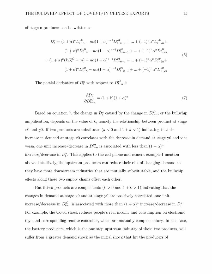
THE BULLWHIP EFFECT OF COVID-19 IN CHINESE EXPORTS 15
of stage n producer can be written as
Dnt = (1 + α)nDx0
t−n − nα(1 + α)n−1Dx0t−n−1 + ...+ (−1)nαnDx0
t−2n+
(1 + α)nDy0t−n − nα(1 + α)n−1Dy0
t−n−1 + ...+ (−1)nαnDy0t−2n
= (1 + α)n(kDy0t +m) − nα(1 + α)n−1Dx0
t−n−1 + ...+ (−1)nαnDx0t−2n+
(1 + α)nDy0t−n − nα(1 + α)n−1Dy0
t−n−1 + ...+ (−1)nαnDy0t−2n
(6)
The partial derivative of Dnt with respect to Dy0
t−n is
∂Dnt
∂Dy0t−n
= (1 + k)(1 + α)n (7)
Based on equation 7, the change in Dnt caused by the change in Dy0
t−n, or the bullwhip
amplification, depends on the value of k, namely the relationship between product at stage
x0 and y0. If two products are substitutes (k < 0 and 1 + k < 1) indicating that the
increase in demand at stage x0 correlates with the decrease in demand at stage y0 and vice
versa, one unit increase/decrease in Dy0t−n is associated with less than (1 + α)n
increase/decrease in Dnt . This applies to the cell phone and camera example I mention
above. Intuitively, the upstream producers can reduce their risk of changing demand as
they have more downstream industries that are mutually substitutable, and the bullwhip
effects along these two supply chains offset each other.
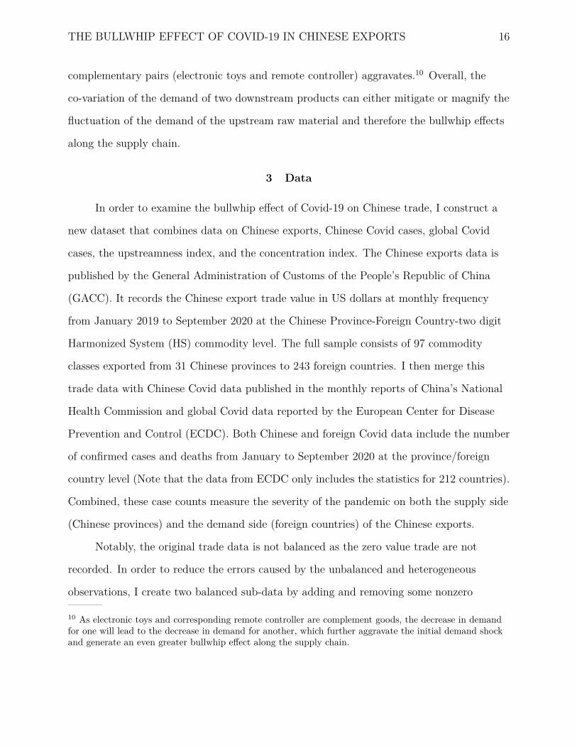
But if two products are complements (k > 0 and 1 + k > 1) indicating that the
changes in demand at stage x0 and at stage y0 are positively correlated, one unit
increase/decrease in Dy0t−n is associated with more than (1 + α)n increase/decrease in Dn
t .
For example, the Covid shock reduces people’s real income and consumption on electronic
toys and corresponding remote controller, which are mutually complementary. In this case,
the battery producers, which is the one step upstream industry of these two products, will
suffer from a greater demand shock as the initial shock that hit the producers of
THE BULLWHIP EFFECT OF COVID-19 IN CHINESE EXPORTS 16
complementary pairs (electronic toys and remote controller) aggravates.10 Overall, the
co-variation of the demand of two downstream products can either mitigate or magnify the
fluctuation of the demand of the upstream raw material and therefore the bullwhip effects
along the supply chain.
3 Data
In order to examine the bullwhip effect of Covid-19 on Chinese trade, I construct a
new dataset that combines data on Chinese exports, Chinese Covid cases, global Covid
cases, the upstreamness index, and the concentration index. The Chinese exports data is
published by the General Administration of Customs of the People’s Republic of China
(GACC). It records the Chinese export trade value in US dollars at monthly frequency
from January 2019 to September 2020 at the Chinese Province-Foreign Country-two digit
Harmonized System (HS) commodity level. The full sample consists of 97 commodity
classes exported from 31 Chinese provinces to 243 foreign countries. I then merge this
trade data with Chinese Covid data published in the monthly reports of China’s National
Health Commission and global Covid data reported by the European Center for Disease
Prevention and Control (ECDC). Both Chinese and foreign Covid data include the number
of confirmed cases and deaths from January to September 2020 at the province/foreign
country level (Note that the data from ECDC only includes the statistics for 212 countries).
Combined, these case counts measure the severity of the pandemic on both the supply side
(Chinese provinces) and the demand side (foreign countries) of the Chinese exports.
Notably, the original trade data is not balanced as the zero value trade are not
recorded. In order to reduce the errors caused by the unbalanced and heterogeneous
observations, I create two balanced sub-data by adding and removing some nonzero
10 As electronic toys and corresponding remote controller are complement goods, the decrease in demandfor one will lead to the decrease in demand for another, which further aggravate the initial demand shockand generate an even greater bullwhip effect along the supply chain.
THE BULLWHIP EFFECT OF COVID-19 IN CHINESE EXPORTS 17
trades.11 The first one has 5 million observations and includes all the zero value trades of
commodity k exporting from province p to foreign country j from 2019 to 2020 as long as
at least one nonzero value trade exists.12 The second one focuses on
province-country-commodity pairs for which I observe positive Chinese exports in every
sample period. This reduces the number of observations to 0.9 million. In this paper, I
primarily focus on the second trade data and my baseline estimates are proved to be robust
using the first trade data that includes more nonzero trades.13
The upstreamness index data comes from Antràs, Chor, Fally, and Hillberry (2012)
who measure the upstreamness index of different industries in the United States and
examine the applicability of the index to other countries. Due to the unavailability of
Chinese upstreamness data, I assume that the inter-industrial connections are similar in
different countries (i.e. the battery producers always export to the electronics producers
and the tire producers always export to car makers) and therefore the upstreamness index
from Antràs et al. (2012) can be applied to Chinese manufacturing sectors. The
concentration index is derived from the Input-Output table published by the Eora Global
Supply Chain Database in 2015 through the normalised Hirschman Herfindahl
concentration index calculation provided by Zavacka (2012).14 To merge the trade data
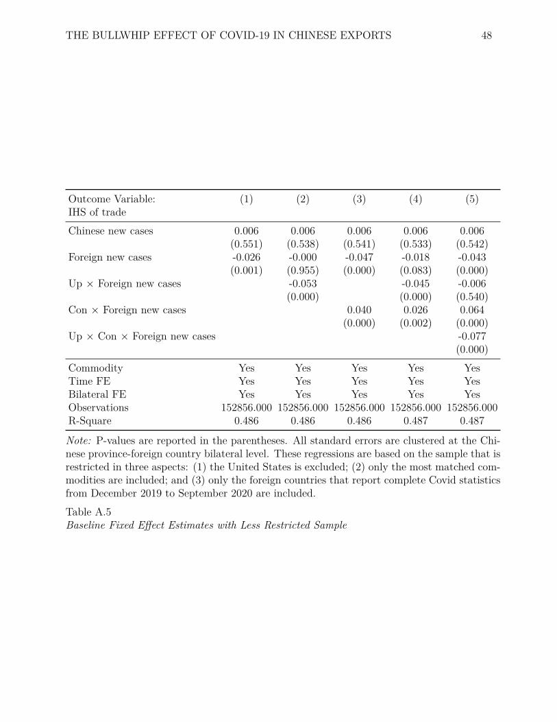
with the upstreamness index and concentration index, I build two crosswalks between the
industries and traded commodities. There are 57 matched commodities and 16 perfect
11 In order to construct a balanced panel data, I create a template at the Chinese Province-ForeignCountry-two digit Harmonized System (HS) commodity level that includes all the possible trades andmerge it to the trade data to create zero trades.12 For example, if Beijing exports $694, 156 of article of iron or steel to Bahrian in July 2019 and there isno trades of article of iron or steel from Beijing to Bahrian in the rest of the months from 2019 to 2020, Iwill still incorporate the zero value trades in these months.13 The coefficients of interest (the foreign new cases, the interaction term between upstreamness binary andforeign new cases, and the interaction term between concentration binary and foreign new cases) inTable A.5 are generally consistent with my baseline estimates in Table 4.14 The equation provided by Zavacka (2012) is Ci =
∑N
j=1s2
ij− 1N
1− 1N
where sij denotes the production share ofindustry i contributes to industry j relative to total production of industry i. The final normalizationconcentration index will vary between zero and one, with one indicating that the products of certainindustry are only targeting one downstream industry.
THE BULLWHIP EFFECT OF COVID-19 IN CHINESE EXPORTS 18
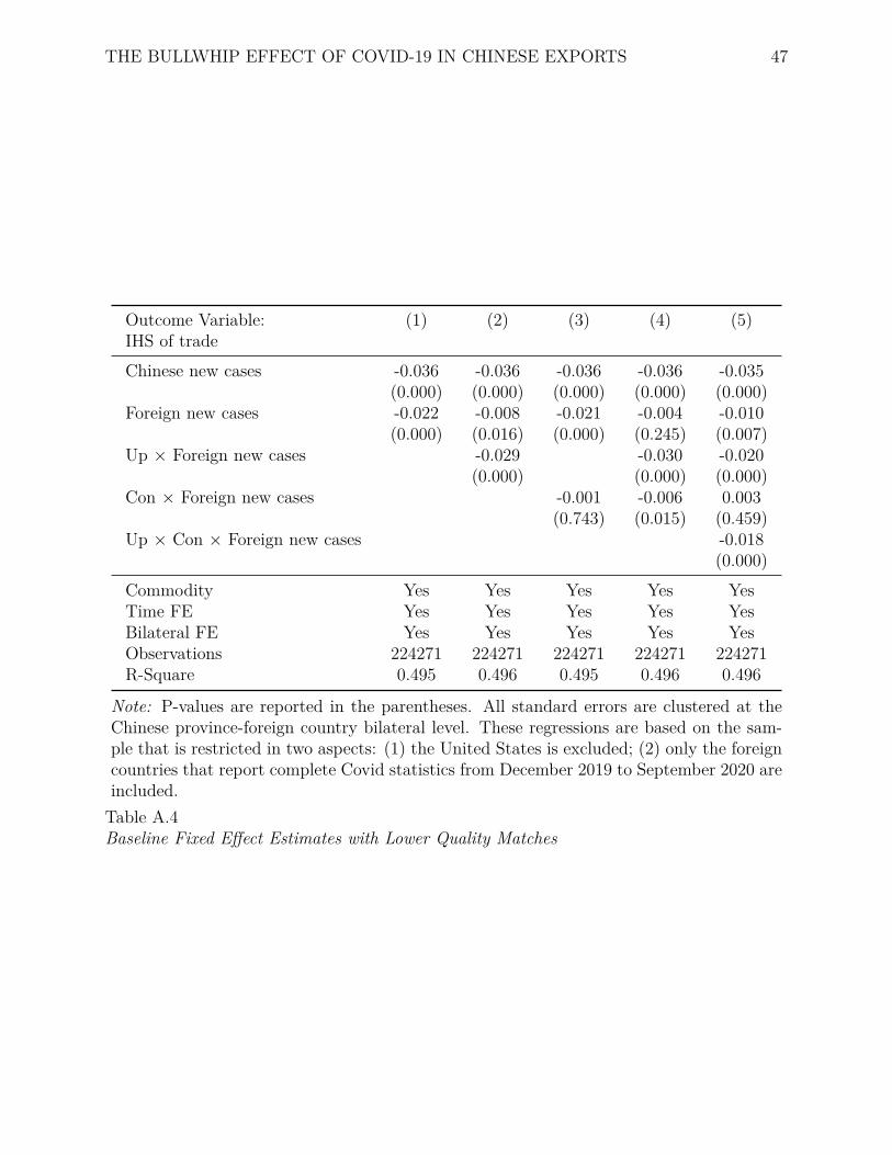
matches. While the primary analyses are based on the data with only the 16 perfect
matches, the empirical results with all 57 matched commodities15 shown in Table A.4 are
generally consistent with my baseline estimates presented in Table 4.
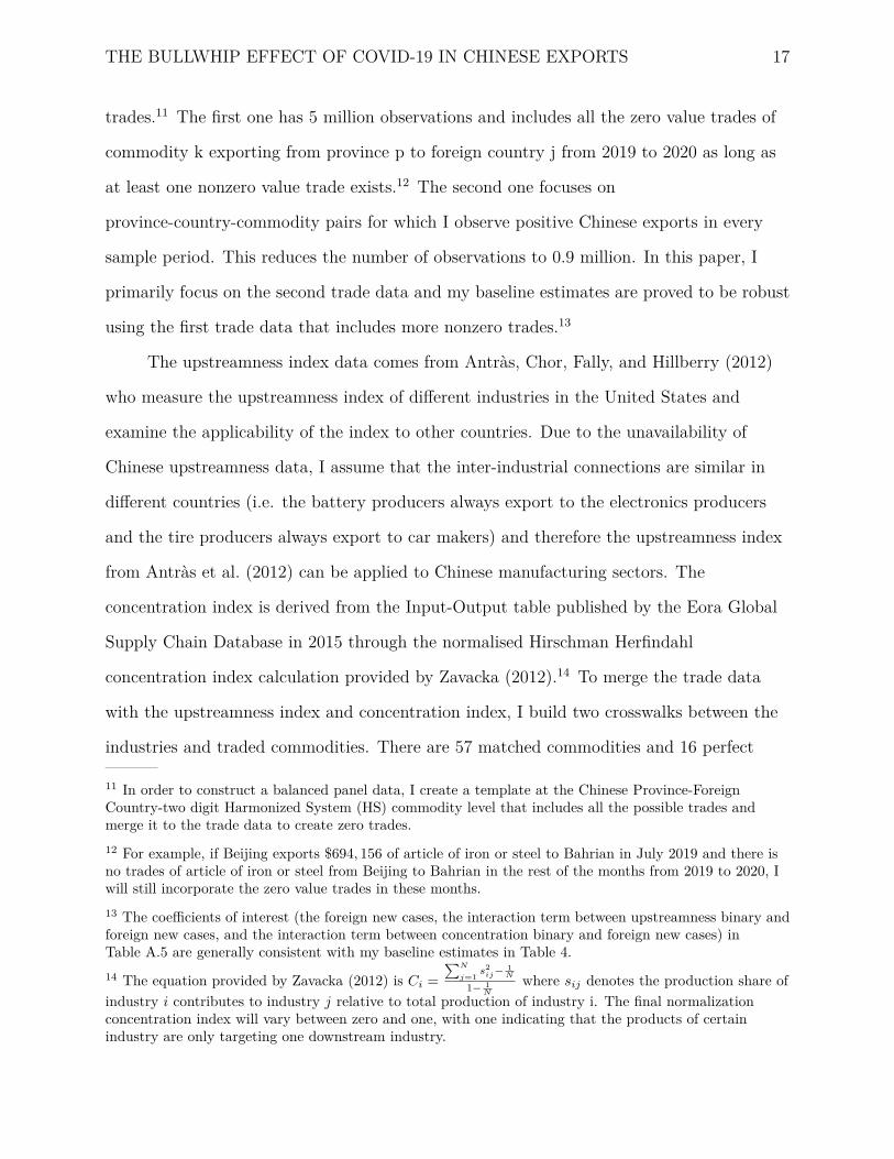
Variables Mean Median Std Deviation Min Max NTrade(2019)(mil) 3.04 0.63 8.74 0.00 436 42381Trade(2020)(mil) 2.98 0.57 9.18 0.00 558 42381Chinese new Covid cases 338.40 11.00 3617.82 0.00 59754.00 42381Foreign new Covid cases 52095.01 2975.00 224834.21 0.00 2604518.00 42381Upstreamness index 2.46 2.49 0.89 1.06 3.96 16Concentration index 0.27 0.26 0.15 0.03 0.53 16
Table 2Summary Statistics: Trade Value, New Covid Cases, and Upstreamness and ConcentrationIndex
3.1 Trade Value and Covid Cases
The outcome variable of interest is represented by the volume of Chinese exports,
which measures the demand of foreign countries. Table 2 shows the summary statistics of
the trade volume in 2019 and 2020, Chinese and foreign new Covid cases, and
upstreamness and concentration index. Note that the statistics include 29 provinces and 62
foreign countries that have complete trade and Covid data and 16 commodities that have
quality upstreamness and concentration index.
The mean and median trade value in 2019 are 2.01% and 10.53% higher than those in
2020, indicating the trade disruption generated by Covid-19. The standard deviation of
Chinese new cases is significantly greater than the mean and the median. Combined with
the fact that Hubei had approximately sixty thousands maximum monthly cases in
February 2020, it is inferable that Chinese monthly new cases vary a lot by time and
province and the pandemic is concentrated in several provinces like Hubei, Guangdong,
and Heilongjiang in certain months. Also, the mean of Chinese new cases is much greater
than the median, suggesting that the distribution of new cases is strongly right skewed.
15 Two concordance tables are available upon request (email: [email protected]).
THE BULLWHIP EFFECT OF COVID-19 IN CHINESE EXPORTS 19
The statistics of foreign new cases present the same patterns, that the standard deviation
and the maximum value are far higher than the mean and the median, and the mean
foreign new cases is also greater than the median ones. These imply that a small group of
countries are hit harder by Covid-19 than others in certain months (the foreign new cases
vary a lot by country overtime).
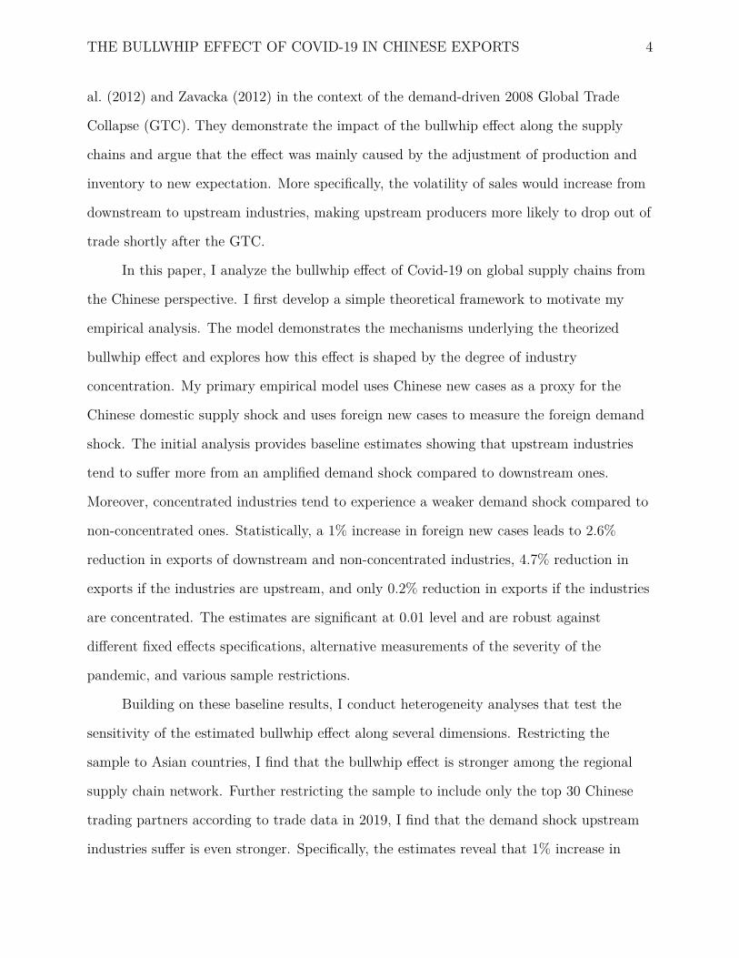
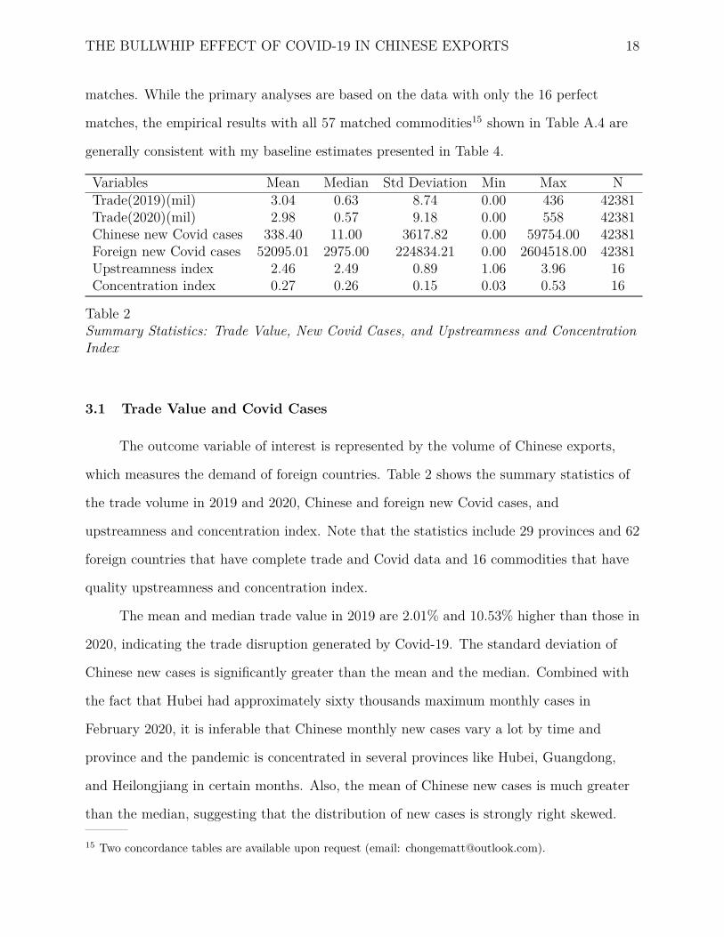
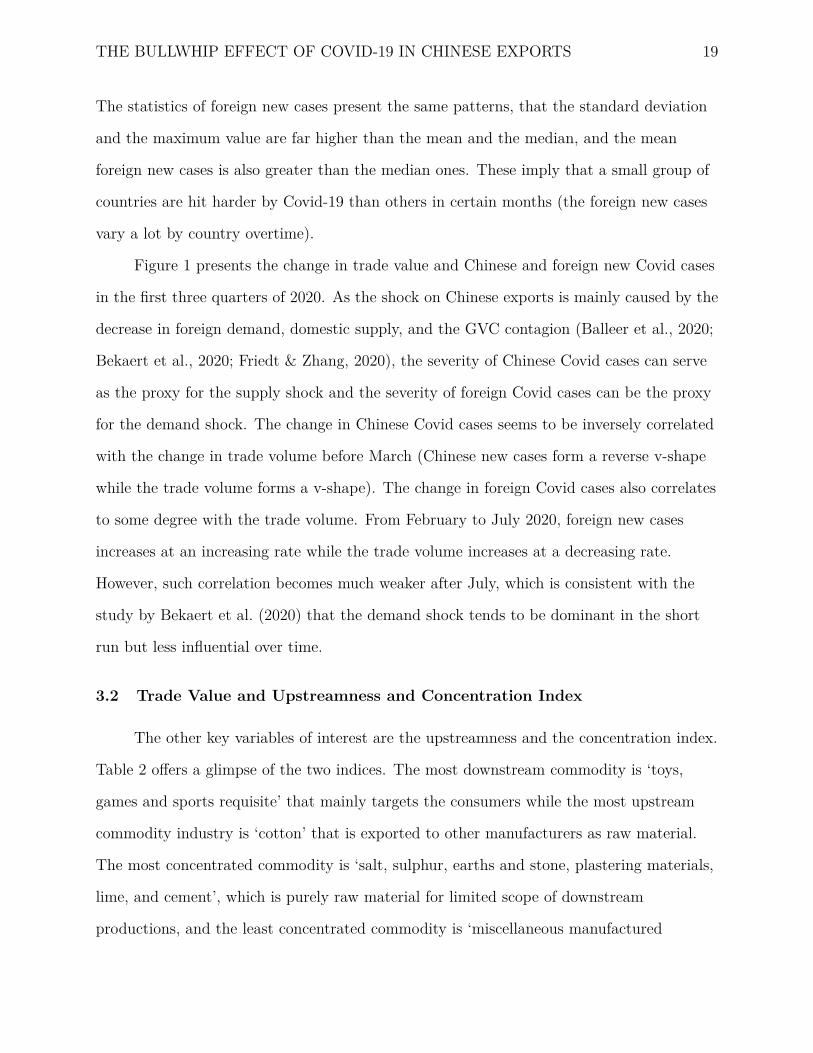
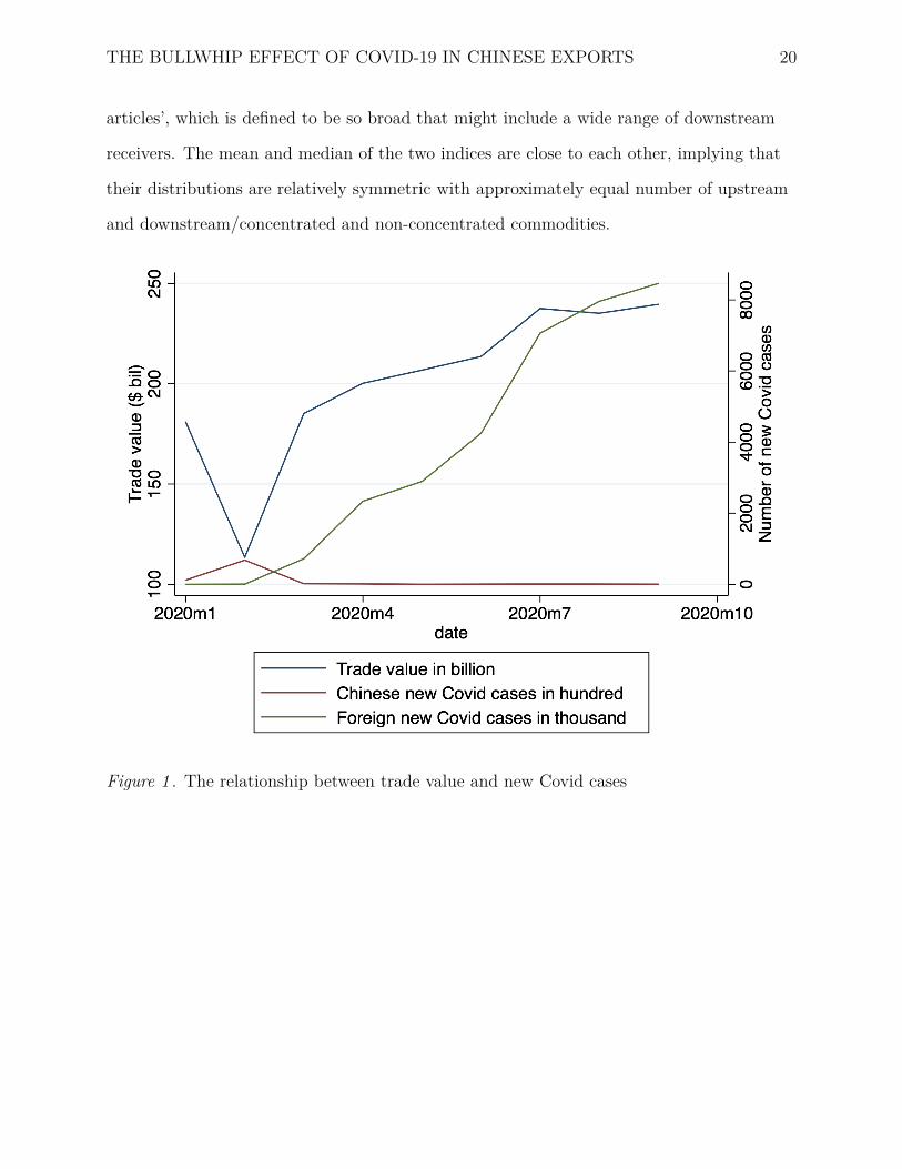
Figure 1 presents the change in trade value and Chinese and foreign new Covid cases
in the first three quarters of 2020. As the shock on Chinese exports is mainly caused by the
decrease in foreign demand, domestic supply, and the GVC contagion (Balleer et al., 2020;
Bekaert et al., 2020; Friedt & Zhang, 2020), the severity of Chinese Covid cases can serve
as the proxy for the supply shock and the severity of foreign Covid cases can be the proxy
for the demand shock. The change in Chinese Covid cases seems to be inversely correlated
with the change in trade volume before March (Chinese new cases form a reverse v-shape
while the trade volume forms a v-shape). The change in foreign Covid cases also correlates
to some degree with the trade volume. From February to July 2020, foreign new cases
increases at an increasing rate while the trade volume increases at a decreasing rate.
However, such correlation becomes much weaker after July, which is consistent with the
study by Bekaert et al. (2020) that the demand shock tends to be dominant in the short
run but less influential over time.
3.2 Trade Value and Upstreamness and Concentration Index
The other key variables of interest are the upstreamness and the concentration index.
Table 2 offers a glimpse of the two indices. The most downstream commodity is ‘toys,
games and sports requisite’ that mainly targets the consumers while the most upstream
commodity industry is ‘cotton’ that is exported to other manufacturers as raw material.
The most concentrated commodity is ‘salt, sulphur, earths and stone, plastering materials,
lime, and cement’, which is purely raw material for limited scope of downstream
productions, and the least concentrated commodity is ‘miscellaneous manufactured
THE BULLWHIP EFFECT OF COVID-19 IN CHINESE EXPORTS 20
articles’, which is defined to be so broad that might include a wide range of downstream
receivers. The mean and median of the two indices are close to each other, implying that
their distributions are relatively symmetric with approximately equal number of upstream
and downstream/concentrated and non-concentrated commodities.
Figure 1 . The relationship between trade value and new Covid cases
THE BULLWHIP EFFECT OF COVID-19 IN CHINESE EXPORTS 21
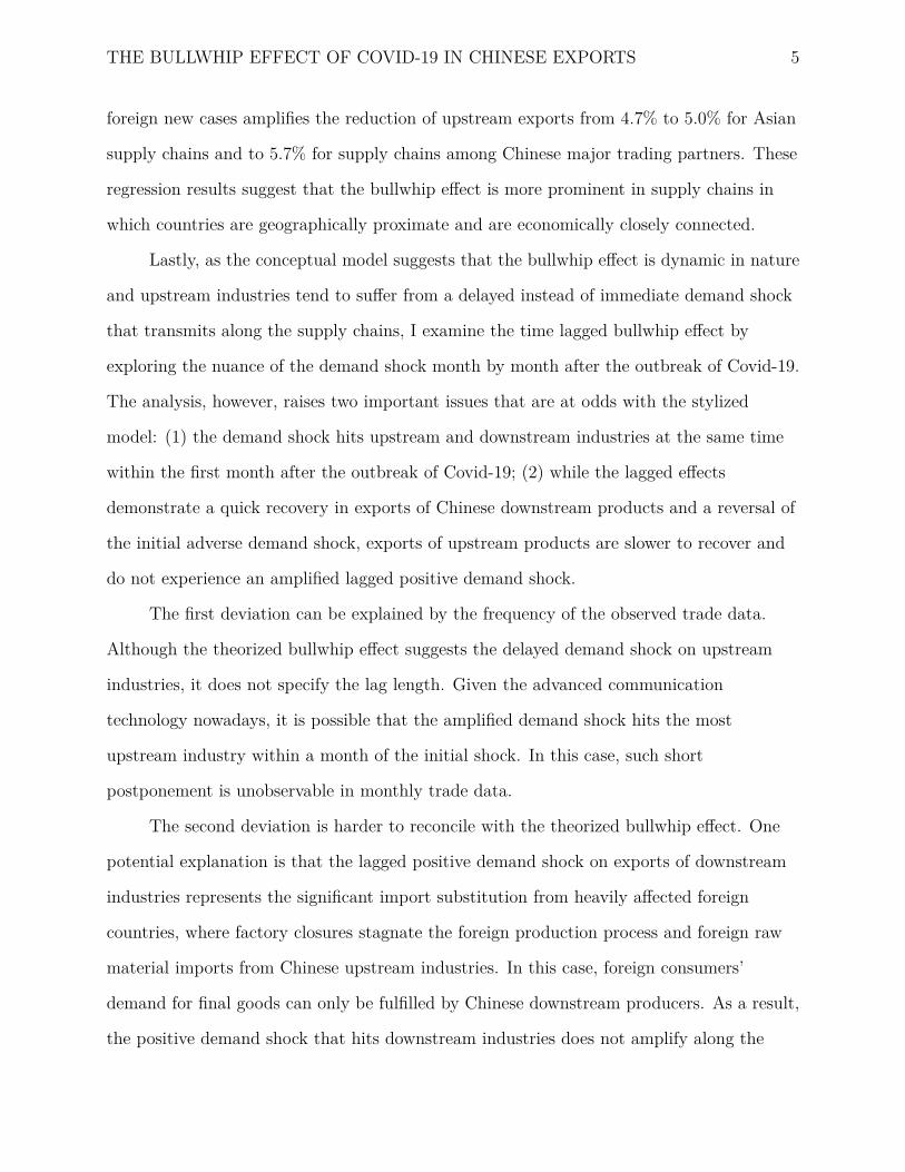
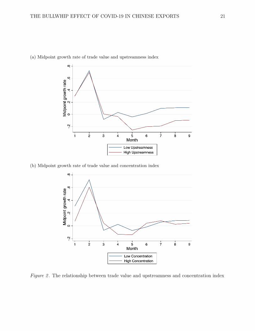
(a) Midpoint growth rate of trade value and upstreamness index
(b) Midpoint growth rate of trade value and concentration index
Figure 2 . The relationship between trade value and upstreamness and concentration index
THE BULLWHIP EFFECT OF COVID-19 IN CHINESE EXPORTS 22
Com
mod
ityUpstreamne
ssCon
centratio
nEx
posure
toEx
posure
toinde
xinde
xChine
seCovid
infection
foreignCovid
infection
Toys,g
ames
andsports
requ
isites;
partsan
daccessoriesthereof
1.058
0.451
11777
6489197
Beverages,s
pirit
san
dvine
gar
1.266
0.242
70.55
7590
Toba
ccoan
dman
ufacturedtoba
ccosubstit
utes
1.581
0.276
50.45
6477
Ceram
ic1.727
0.503
4194
1660892
Ships,
boatsan
dflo
atingstructures
1.818
0.226
144.4
126718
Pharmaceu
tical
prod
ucts
1.982
0.311
8928
1625681
Railway
ortram
way
locomotives,r
ollin
gstock,
fixturesan
dfittin
gs,a
ndpa
rtsthereof;
2.234
0.336
2425
449402
mecha
nicaltrafficsig
nalin
gequipm
entof
allk
inds
Glass
andglassw
are
2.476
0.109
4038
1783320
Sugars
andsugarconfectio
nery
2.506
0.197
113.7
65900
Dairy
prod
uct;eggs;n
atural
hone
y;ed
ible
prod
ucts
ofan
imal
2.554
0.262
460.4
4687
Rub
beran
dartic
lesthereof
2.741
0.0308
3833
2066729
Plastic
san
dartic
lesthereof
2.801
0.0390
24820
9262688
Cereals
3.109
0.157
3.049
76.74
Fertilizers
3.762
0.533
9614
468034
Iron
andsteel
3.854
0.346
14859
2493056
Cotton
3.964
0.261
600.8
389959
Upstream
commod
ities
6788.046
1843891
Dow
nstream
commod
ities
3953.329
1518660
Con
centratedcommod
ities
6538.436
1649678
Non
-con
centratedcommod
ities
4202.939
1712873
Not
e:The
names
ofthecommod
ityareab
breviatedan
dtheorde
ris
sorted
bytheup
stream
ness
inde
x.The
expo
sure
iscalculated
byΣ
(Per
cen
tEx
por
ts∗
New
Case
s)whe
reP
erce
ntE
xpor
tsde
notesthepe
rcentage
ofexpo
rtsof
thecommod
ityby
each
Chine
seprovin-
cial/foreign
coun
tryan
dN
ewC
ase
sde
notesthenu
mbe
rof
new
casesof
theChine
seprovince/foreign
coun
try.
The
benchm
arkto
split
upstream
anddo
wnstream,c
oncentratedan
dno
n-conc
entrated
indu
strie
sis
themedianof
thetw
oindices.
Highexpo
sure
means
that
the
commod
ityis
potentially
moreaff
ectedby
theCovid-19infection.
Table3
Trad
eexposure
toChine
sean
dforeignCovid
infectionof
theperfectly
matched
commodities
THE BULLWHIP EFFECT OF COVID-19 IN CHINESE EXPORTS 23
Figure 2 presents the relationships between the midpoint growth rate16 of trade value
and the two indices. Both relationships are consistent with the theoretical model in Section
2. Note that I use the midpoint growth rate instead of the trade volume because the
midpoint growth rate that uses the trade volumes last year as benchmarks provides a
better visualization of Covid shock compared to the seasonally fluctuated absolute value of
trade volume. In Figure 2a, commodities from upstream industries (labeled as high
upstreamness) tend to be more volatile than those from downstream industries (labeled as
low upstreamness) as the drop of midpoint growth rate is more drastic since April 2020.17
In Figure 2b, the changes in midpoint growth rate are similar for commodities from
concentrated and non-concentrated industries, meaning that the effect of industry
concentration on trade is ambiguous.18 These two visualizations support the conclusions
drawn from the conceptual bullwhip effect.
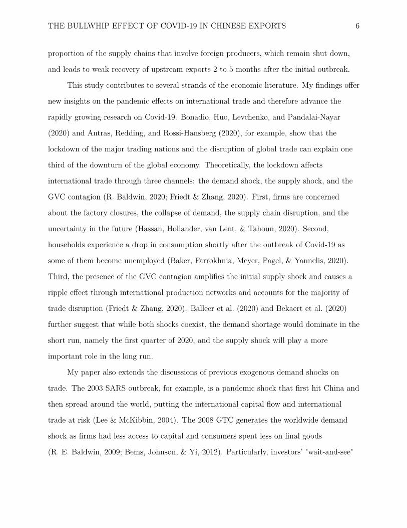
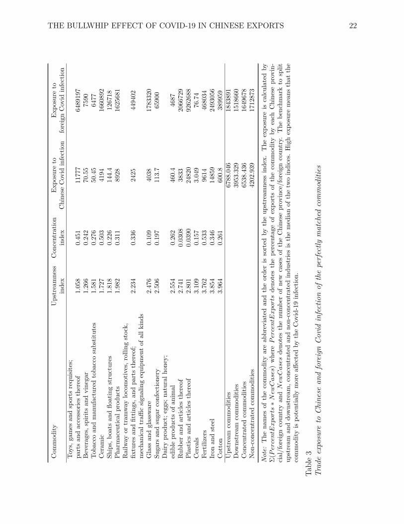
Table 3 further reveals the Covid shock on the final 16 Chinese export commodities.19
from the perspective of trade exposure to Chinese domestic and foreign Covid infection.
The trade exposures are calculated as the weighted sum of new cases in Chinese
provinces/foreign countries where the weights are given by the share of exports from each
province/share of imports to each country in 2020. It measures the extent to which a
particular commodity is exposed to Chinese domestic and foreign Covid-19 pandemic.
Suppose, for instance, the United States imports all Chinese iron and steel but only 50% of
16 The midpoint growth rate is calculated by T radepjkt−T radepjkt−120.5∗(T radepjkt+T radepjkt−12) where Tradepjkt denotes the trade
volume of commodity k from province p to foreign country j at time t. t − 12 denotes the time one yearbefore. The midpoint growth rate of trade value is developed by Bricongne, Fontagné, Gaulier, Taglioni,and Vicard (2010) and can correctly approximate the aggregate growth rate of exports and overcome theseasonality bias.17 I categorize commodities with upstreamness index smaller than the median to be low upstreamness andthat greater than the median to be high upstreamness.18 I categorize commodities with concentration index smaller than 0.5 to be low concentration and thatgreater than 0.5 to be high concentration. 0.5 is calculated by the median of the two possible extremes,zero and one.19 These 16 commodities have perfectly matched upstreamness and concentration index and will be themain focus of my following empirical section.
THE BULLWHIP EFFECT OF COVID-19 IN CHINESE EXPORTS 24
fertilizers. If all the foreign new cases are in the United States, the iron and steel industry
faces a stronger foreign demand shock than the fertilizers industry.
By splitting upstream and downstream, concentrated and non-concentrated
industries based on the median of the two indices, I find that upstream industries tend to
have more exposures to Covid infections both domestically and internationally while
concentrated industries tend to expose more to domestic but less to foreign infections. In
other words, the export provinces and import foreign countries of upstream commodities
are hit harder by Covid-19, and the export provinces of concentrated commodities and the
import foreign countries of non-concentrated commodities have relatively more severe
pandemic. Although the results cannot apply universally to every commodity, the general
trend they reflect is consistent with the results from Figure 2. Note that the higher trade
exposure of upstream industries does not directly indicate the bullwhip effect but just shed
light upon the potential Covid impact on different commodities. The bullwhip effect is
demonstrated in the following Section 4 using a fixed effects model to control for province,
foreign country, commodity, and time unobservables.
4 Empirical Result
In order to empirically test the bullwhip effect along the global supply chains from
the Chinese perspective, I choose to use a fixed effect model to soak up the average
difference across province-foreign country bilateral relations, commodity, and time. The
sample of my baseline estimates is restricted in three ways: (1) the United States is
excluded because the ongoing trade war might affect the empirical result;20 (2) only the
perfectly matched commodities in the data concordance are included; and (3) only the
foreign countries that report complete Covid statistics from December 2019 to September
20 For example, the Phase One trade deal in January 15th, 2020, right after the outbreak of Covid-19 inChina and right before the global outbreak, reduces duties from 15% to 7.5% on $120 billion Chinesecommodities. China also agrees to purchase at least an additional $200 billion worth of US commoditiesaccording to the trade deal. In this case, the deal will affect the import and export of Chinese productsand therefore the trade volume within the supply chain.
THE BULLWHIP EFFECT OF COVID-19 IN CHINESE EXPORTS 25
2020 are included. My baseline results demonstrate the significance of the bullwhip effect,
suggesting that upstream industries tend to suffer from a greater demand shock measured
by the volume of exports compared to the downstream industries. I then test the
sensitivity of my baseline results against alternative measures of the Covid shock, different
fixed effect specifications, and various sample restrictions. Following the baseline analyses,
I explore the dynamics of the hypothesized bullwhip effect on Chinese exports and estimate
the time lagged effects of COVID-19 along the supply chain, which points to some
discrepancies between the theory and the data.
4.1 Baseline Estimates
The baseline estimates are based on a fixed effects specification that models Chinese
Exports (X) as a function of domestic Covid case counts (DC) and foreign case counts
(FC) while controlling for bilateral province-foreign country pairs (αpj) as well as
time-invariant differences across commodities (ρk) and common time trends and seasonal
variation (µt). To investigate the potential bullwhip effect along the supply chain and shed
light on the influence of industry concentration, I interact foreign country cases with
indicator variables that differentiate industries with below and above median upstreamness
(UP ) or concentration (CON). The standard errors are clustered at the province-foreign
country bilateral level. The resulting specification can be described as follows:
Xpjkt = β0 + β1DCpt + β2FCjt + β3FCjt ∗ UPk+
β4FCjt ∗ CONk + αpj + ρk + µt + εpjkt (8)
where Xpjkt is the inverse hyperbolic sine (IHS) transformation of the volume of
export of commodity k from province p to foreign country j at time t.21 DCpt measured by
21 While the frequently used logarithm transformation can cluster the extreme values to the middle andreduce their unnecessarily large effects on the empirical results, such transformation does not apply well ontrade data because it cannot deal with zero value trade. In short, ln(0) is undefined. Therefore, I choose touse the IHS to transform my data as zero can be defined.
THE BULLWHIP EFFECT OF COVID-19 IN CHINESE EXPORTS 26
the IHS of Chinese domestic confirmed and death Covid cases at the province level
indicates the severity of Covid-19 in China and serves as a proxy for Chinese domestic
supply shock. FCjt, on the other hand, measured by the IHS of foreign confirmed and
death Covid cases at the foreign country level represent the international demand shock.
Both DCpt and FCjt are good proxies because the number of Covid cases is closely related
to the factory closures (R. Baldwin et al., 2020) and negatively correlated with consumers’
income and expenditure (Coibion, Gorodnichenko, & Weber, 2020). UPk and CONk are
binary variables that denote whether the commodity is upstream or concentrated
respectively and the benchmark of separation is their median value. I use the binary
instead of the continuous variables because one unit change in either index does not
necessarily generate a linear effect on exports. For example, the difference in Covid shock
between upstream and midstream industries is not necessarily the same as the difference in
Covid shock between midstream and downstream industries.
While β1 indicates the effect of Chinese domestic Covid-led supply shock, the primary
coefficients of interest in equation 8 are β2, β3, and β4, which reflect the direction and
magnitude of foreign Covid-led demand shock on different industries. Specifically, β2
measures the demand shock on non-concentrated, downstream industries; β3 measures the
additional demand shock for exports of upstream industries; and β4 measures the
additional demand shock for exports of concentrated industries. Based on the bullwhip
effect N-stage model in Section 2, I expect β2 and β3 to be negative and significant while β4
is ambiguous. In other words, upstream industries suffer from a greater demand shock than
downstream industries do, and the role concentration plays varies by industries.
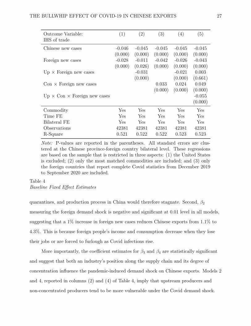
Table 4 shows the baseline coefficient estimates of equation 8. First, β1 measuring the
Chinese domestic supply shock is negative and significant at 0.01 level in all models,
indicating that a 1% increase in Chinese new cases reduces Chinese exports by
approximately 4.5%. This matches with my expectation and the estimates from Friedt and
Zhang (2020) as the spread of Covid-19 would lead to factory closures and workers’
THE BULLWHIP EFFECT OF COVID-19 IN CHINESE EXPORTS 27
Outcome Variable: (1) (2) (3) (4) (5)IHS of tradeChinese new cases -0.046 -0.045 -0.045 -0.045 -0.045
Note: P-values are reported in the parentheses. All standard errors are clus-tered at the Chinese province-foreign country bilateral level. These regressionsare based on the sample that is restricted in three aspects: (1) the United Statesis excluded; (2) only the most matched commodities are included; and (3) onlythe foreign countries that report complete Covid statistics from December 2019to September 2020 are included.
Table 4Baseline Fixed Effect Estimates
quarantines, and production process in China would therefore stagnate. Second, β2
measuring the foreign demand shock is negative and significant at 0.01 level in all models,
suggesting that a 1% increase in foreign new cases reduces Chinese exports from 1.1% to
4.3%. This is because foreign people’s income and consumption decrease when they lose
their jobs or are forced to furlough as Covid infections rise.
More importantly, the coefficient estimates for β3 and β4 are statistically significant
and suggest that both an industry’s position along the supply chain and its degree of
concentration influence the pandemic-induced demand shock on Chinese exports. Models 2
and 4, reported in columns (2) and (4) of Table 4, imply that upstream producers and
non-concentrated producers tend to be more vulnerable under the Covid demand shock.
THE BULLWHIP EFFECT OF COVID-19 IN CHINESE EXPORTS 28
Specifically, a 1% increase in foreign new cases reduces Chinese exports of downstream
industries by 2.6% and those of upstream industries by 4.7%, suggesting that the bullwhip
effect almost doubles the demand shock along the supply chain. The same unit of change in
foreign new cases rises Chinese concentrated exports by 0.2% and drops non-concentrated
ones by 2.6%, indicating that the Covid shock on non-concentrated industries is more
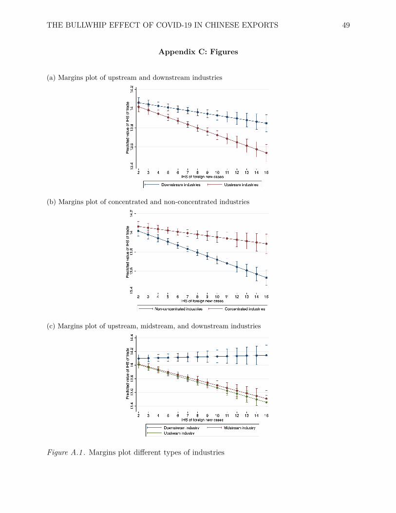
severe. These can also be visualized via the Figure A.1a and Figure A.1b in the Appendix
C that show the predicted value of trade of different types of industries over foreign new
cases, the proxy for foreign demand shock. While the predicted value of trade decreases as
the Covid shock becomes more severe, upstream industries in Figure A.1a and
non-concentrated industries in Figure A.1b apparently experience a steeper drop in trade.
The story becomes more complicated when I add in the triple interaction term
FCjt ∗ UPk ∗ CONk that indicates the joint effect of upstreamness and concentration.
Model 5 in Table 4 shows that in the best case, a 1% increase in foreign new cases does not
really affect Chinese exports of a downstream industry that is concentrated (like
pharmaceutical and signalling equipment producers).22 In the worst case, the same change
in foreign new cases will drop Chinese exports by almost 10% for an upstream industry
that is concentrated (like fertilizers and iron and steel producers).23
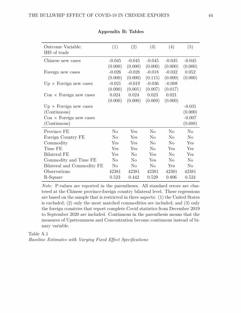
4.2 Robustness Checks and Heterogeneous Analysis
Table A.1 in Appendix B shows the empirical result with different fixed effect
specifications. By controlling for province, foreign country, commodity, and time fixed
effects individually or with some of them interacted with each other, the baseline results
still hold. Model 2 through 4 show that upstream industries still suffer from an amplified
negative shock compared to downstream industries (indicated by the negative sign of the
interaction term between upstreamness and foreign new cases) and the size of amplification
22 The effect is calculated by −0.043 + 0.049 = 0.006.23 The effect is calculated by −0.043 − 0.055 = −0.098.
THE BULLWHIP EFFECT OF COVID-19 IN CHINESE EXPORTS 29
depends on the fixed effect specifications. Concentrated industries also experience a weaker
demand shock provided by the positive coefficient of the interaction between concentration
binary and foreign new cases.
In order to visualize more nuances between industries, I split the upstreamness index
into terciles.24 Figure A.1c in Appendix C presents the predicted value of trade of
downstream, midstream, and upstream industries over foreign new cases. The trend-line
shows clearly that the Covid shock is greater on upstream and midstream industries
compared to the downstream ones while the gap between upstream and midstream
industries is not significant, which is consistent with my baseline results. Model 5 in
Table A.1 further shows the coefficients when upstreamness and concentration index are
continuous. While upstream industries still experience an amplified demand shock, the
shock on concentrated and non-concentrated industries is numerically similar given that
the coefficient of the interaction term between concentration index and foreign new cases
approaches zero and the p-value exceeds 0.05. However, as I mention above that the
continuous upstreamness and concentration index cannot generate a reliable result, model
9 only serves as a robustness check for my baseline estimates.
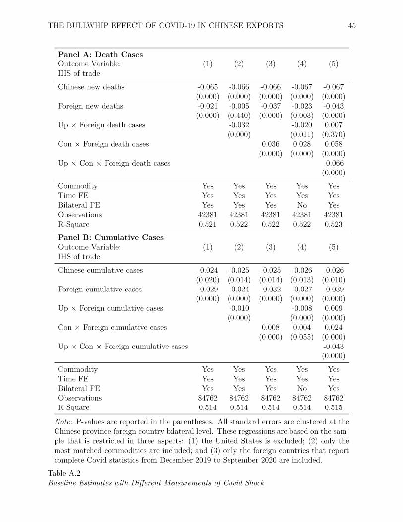
Table A.2 in Appendix B presents the estimates when I change the measurement of
the Covid shock from new cases to death cases (see Panel A) and cumulative cases (see
Panel B). While all three measurements represent slightly different aspects of the severity
of Covid-19 (new and cumulative cases indicate the spread while death cases reveal the
fatality of the pandemic), the signs of coefficients are consistent with my baseline estimates.
Additionally, I test the sensitivity of my estimates against alternative sample
restrictions by, for example, including the United States or expanding the set of exported
commodities to include less well matched commodities. Panel A in Table A.3, Table A.5,
Table A.4 in Appendix B show the estimates under these relaxed sample restrictions. The
magnitudes and signs of the three coefficients of interest (β2, β3, and β4) are consistent
24 The benchmark of the split is based on the 33 and 66 percentile of the upstreamness index.
THE BULLWHIP EFFECT OF COVID-19 IN CHINESE EXPORTS 30
with my baseline estimates.25
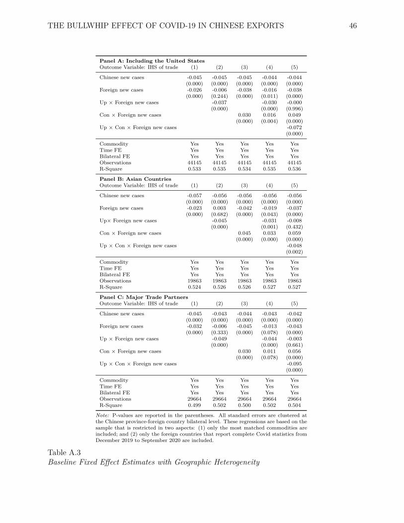
Finally, I explore the heterogeneity of my baseline findings by restricting the sample
to include only Asian countries and only the top 30 Chinese major trading partners.26
While the signs are consistent with my baseline estimates, the coefficients of the interaction
between upstreamness binary and foreign new cases in Panel B and Panel C in Table A.3
in Appendix B are numerically 1% greater than that in my baseline result. Specifically, for
a 1% increase in foreign new cases, the additional shock on upstream industries is 50%
greater for trade among Asian countries and 100% greater for trade among the top trading
partners, suggesting that the bullwhip effect tends to be stronger in regional supply chains
and supply chains in which countries are closely connected.27 Intuitively, this is because
when upstream and downstream producers are closely connected geographically and/or
economically, upstream industries tend to hold more inventory to prevent supply shortages.
In this case, the same unit of change in downstream demand will lead to a greater
fluctuation in inventory adjustment and therefore more volatility in demand for upstream
industries.
4.3 Time Lagged Effect
While the baseline estimates are robust across a number of sensitivity analyses, they
only reveal the the immediate impact of Covid-19 and fail to capture the nuance of the
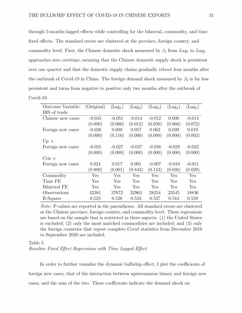
demand shock month by month after the outbreak of Covid-19. Table 5 shows the 1-month
25 The coefficient of the interaction between concentration binary and foreign new cases in Table A.4 thatincludes the less well matched commodities is numerically smaller than my baseline estimates. But becausethe theory suggests that the effect of concentration on trade is ambiguous depending on the type ofindustries, mutually substitute or complement, the numerically smaller coefficients are acceptable.26 These 30 major trading partners occupy almost 70% of Chinese exports and each of them import a hugeamount of industrial goods from China each year. Therefore, their industrial producers should be closelyconnected with Chinese industries.27 Note that numerically (in terms of percentage point) the coefficient of the interaction term betweenupstreamness and foreign new cases increases from 2.1% in the baseline estimates to 3.1% for trade amongAsian countries and 4.4% for trade among Chinese major trading partners. But in terms of the tradevolume, the increase becomes 50% and 100% respectively.
THE BULLWHIP EFFECT OF COVID-19 IN CHINESE EXPORTS 31
through 5-months lagged effects while controlling for the bilateral, commodity, and time
fixed effects. The standard errors are clustered at the province, foreign country, and
commodity level. First, the Chinese domestic shock measured by β1 from Lag1 to Lag5
approaches zero overtime, meaning that the Chinese domestic supply shock is persistent
over one quarter and that the domestic supply chains gradually reboot four months after
the outbreak of Covid-19 in China. The foreign demand shock measured by β2 is far less
persistent and turns from negative to positive only two months after the outbreak of
Covid-19.
Outcome Variable: (Original) (Lag1) (Lag2) (Lag3) (Lag4) (Lag5)IHS of tradeChinese new cases -0.045 -0.051 -0.014 -0.012 0.000 -0.014
(0.000) (0.001) (0.843) (0.143) (0.046) (0.029)Commodity Yes Yes Yes Yes Yes YesTime FE Yes Yes Yes Yes Yes YesBilateral FE Yes Yes Yes Yes Yes YesObservations 42381 37672 32963 28254 23545 18836R-Square 0.523 0.526 0.533 0.537 0.544 0.559Note: P-values are reported in the parentheses. All standard errors are clusteredat the Chinese province, foreign country, and commodity level. These regressionsare based on the sample that is restricted in three aspects: (1) the United Statesis excluded; (2) only the most matched commodities are included; and (3) onlythe foreign countries that report complete Covid statistics from December 2019to September 2020 are included.
Table 5Baseline Fixed Effect Regressions with Time Lagged Effect
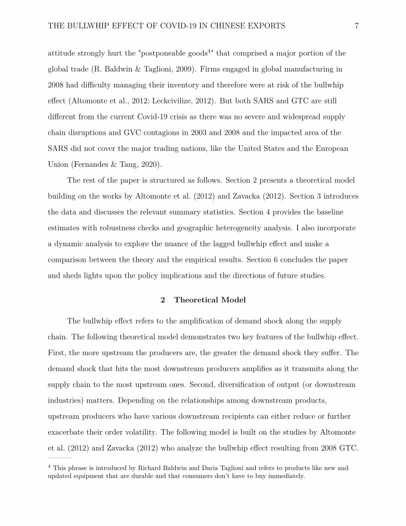
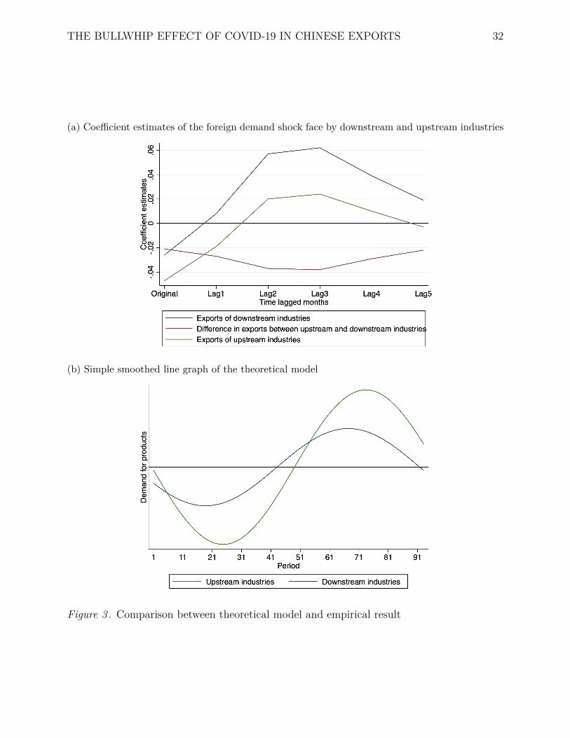
In order to further visualize the dynamic bullwhip effect, I plot the coefficients of
foreign new cases, that of the interaction between upstreamness binary and foreign new
cases, and the sum of the two. These coefficients indicate the demand shock on
THE BULLWHIP EFFECT OF COVID-19 IN CHINESE EXPORTS 32
(a) Coefficient estimates of the foreign demand shock face by downstream and upstream industries
(b) Simple smoothed line graph of the theoretical model
Figure 3 . Comparison between theoretical model and empirical result
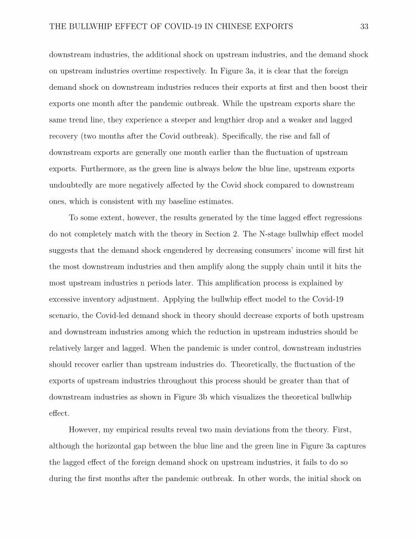
THE BULLWHIP EFFECT OF COVID-19 IN CHINESE EXPORTS 33
downstream industries, the additional shock on upstream industries, and the demand shock
on upstream industries overtime respectively. In Figure 3a, it is clear that the foreign
demand shock on downstream industries reduces their exports at first and then boost their
exports one month after the pandemic outbreak. While the upstream exports share the
same trend line, they experience a steeper and lengthier drop and a weaker and lagged
recovery (two months after the Covid outbreak). Specifically, the rise and fall of
downstream exports are generally one month earlier than the fluctuation of upstream
exports. Furthermore, as the green line is always below the blue line, upstream exports
undoubtedly are more negatively affected by the Covid shock compared to downstream
ones, which is consistent with my baseline estimates.
To some extent, however, the results generated by the time lagged effect regressions
do not completely match with the theory in Section 2. The N-stage bullwhip effect model
suggests that the demand shock engendered by decreasing consumers’ income will first hit
the most downstream industries and then amplify along the supply chain until it hits the
most upstream industries n periods later. This amplification process is explained by
excessive inventory adjustment. Applying the bullwhip effect model to the Covid-19
scenario, the Covid-led demand shock in theory should decrease exports of both upstream
and downstream industries among which the reduction in upstream industries should be
relatively larger and lagged. When the pandemic is under control, downstream industries
should recover earlier than upstream industries do. Theoretically, the fluctuation of the
exports of upstream industries throughout this process should be greater than that of
downstream industries as shown in Figure 3b which visualizes the theoretical bullwhip
effect.
However, my empirical results reveal two main deviations from the theory. First,
although the horizontal gap between the blue line and the green line in Figure 3a captures
the lagged effect of the foreign demand shock on upstream industries, it fails to do so
during the first months after the pandemic outbreak. In other words, the initial shock on
THE BULLWHIP EFFECT OF COVID-19 IN CHINESE EXPORTS 34
upstream industries might be simultaneous with, instead of lagged behind, the shock on
downstream industries. Second, the exports of Chinese upstream and downstream
industries first decrease up to 2.6% (downstream industries) and 4.7% (upstream
industries) and then start to increase to at most 6.2% (downstream industries) and 2.5%
(upstream industries) for every 1% change in foreign new cases, meaning that the growing
foreign new cases reverses the initial Covid-led export reduction. Also, when downstream
industries recover and their exports increase one month after the outbreak of Covid-19, the
fluctuation of the upstream exports is not as large as the model in Figure 3b predicts.
That is, the green line doesn’t surpass the blue line due to excessive inventory adjustment.
The first deviation can be explained by the rapid information flow along the supply
chain given the advanced communication technology nowadays. Because bilateral trades
are recorded at the monthly frequency, it is possible that upstream industries have already
adjusted their inventory within the first month after the pandemic outbreak. In other
words, although the shock in theory takes n period to transmit from the most downstream
to the most upstream industry, in practice n periods might be shorter than a month.
The second deviation can be attributed to the import substitution. In detail, the
theory, although it explains the bullwhip effect on supply chains, does not capture factors
like foreign factory, especially upstream factory, closures that generate the import
substitution, which boosts Chinese downstream exports and drags down upstream exports.
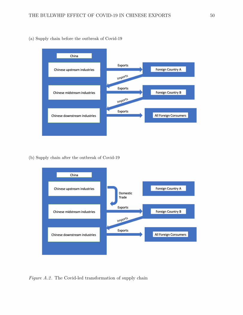
Figure A.2 in Appendix C shows a simple example of the transformation of supply chain
due to the Covid-led import substitution. Before the pandemic outbreak, the whole supply
chain lies across China and Foreign Country A and B and eventually fulfill all foreign
demand by Chinese downstream final goods producers. The global pandemic outbreak
reduces foreign consumers’ income and therefore Chinese downstream exports to all foreign
consumers, which, according to the bullwhip effect theory, also reduces Chinese upstream
exports due to inventory adjustments.
However, shortly after the outbreak, as industrial production in Foreign Country A is
THE BULLWHIP EFFECT OF COVID-19 IN CHINESE EXPORTS 35
stagnating while the production in China is resuming, consumers in Foreign Country A
have to purchase final goods from Chinese downstream industries for their basic needs.
This import substitution then serves as a positive demand shock at the consumer end of
the supply chain, which increases the exports of both downstream and upstream industries
successively due to the upward inventory adjustment. But note that the stagnating foreign
industrial production also cease the Chinese upstream exports to Foreign Country A as the
pandemic shuts down factories there. The upstream production in Foreign Country A is
temporarily replaced by producers from other countries. The integration of these two
effects therefore explains why the Covid-led demand shock does not reduce Chinese exports
persistently and why the recovery is more prominent in downstream than in upstream
industries.
5 Conclusion
In this paper, I study the bullwhip effect of Covid-19 along the global supply chain
from the Chinese perspective. My baseline estimates suggest that upstream industries tend
to suffer from a stronger negative demand shock compared to downstream industries while
concentrated industries in vast majority of the cases tend to have a weaker demand shock,
which is consistent with the bullwhip effect theory. Specifically, a 1% increase in foreign
new cases reduces Chinese exports by 2.6% for downstream industries, 4.7% for upstream
industries, and 5.5% for both upstream and concentrated industries. These results are
robust across different fixed effect specifications, measurements of Covid severity, and
sample restrictions. A heterogeneity analysis indicates that the bullwhip effect tends to be
stronger in the supply chains in which countries are geographically proximate and are more
closely connected in terms of the trade volume.
A dynamic analysis of the bullwhip effect, however, indicates some deviations from
the theory. On one hand, the bullwhip effect model mathematically suggests that upstream
industries tend to face a stronger demand shock at a later time as the inventory
THE BULLWHIP EFFECT OF COVID-19 IN CHINESE EXPORTS 36
adjustments can amplify the shock that takes n period to transmit through the supply
chain. On the other hand, my estimates show that (1) the initial Covid-led demand shock
hits downstream and upstream industries in the same month; (2) the change in exports of
downstream and upstream industries turns from negative to positive, and the fluctuation of
upstream exports is weaker than that of downstream exports, which is at odds with the
bullwhip effect model. While the first deviations can be explained by the frequency of my
trade data and the rapid information transmission given the high-tech communication
technology nowadays, the second one cannot be fully explicated without the supplemental
import substitutions theory. In short, it is the shut-down of foreign industrial production
and the corresponding import substitution that leads to increasing demand for Chinese
downstream final goods and decreasing demand for Chinese upstream raw or intermediate
goods.
My study also sheds light upon the current Covid policies across different countries,
suggesting that the global industrial recovery needs the combination of both demand and
supply side supports from better control of the pandemic. Blindly reopening the economy
is theoretically ineffective. In detail, countries like the United States, India, Brazil, France,
and Italy need to strengthen their Covid-19 prevention measures to handle their over ten
thousand daily new cases in February 2021. When the pandemic is to some extent under
control, industrial production can be normalized (supply side) and consumers’ income can
be recuperated (demand side). In this case, a gradual Covid-prevention accompanying with
economic reopening can not only effectively smooth out the fluctuation generated by the
bullwhip effect but also reduce the inefficiency caused by the import substitution.28
From the global perspective, the regional and international corporation in Covid-19
prevention is also crucial in today’s interconnected world. On one hand, regional trade is
proved to be more volatile based on my heterogeneity analysis of the bullwhip effect, so
28 The import substitution will expose producers to a less internationally competitive environment. Asthey are less likely to select trading partners, the production, communication and transportation might beinefficient.
THE BULLWHIP EFFECT OF COVID-19 IN CHINESE EXPORTS 37
cooperation among East Asian countries, for example, can theoretically promote their
trade recoveries. On the other hand, as international trade accounts for 60.27% of the
world GDP in 2019 according to the World Bank data, world economy and global supply
chains are easily affected by the pandemic as long as it hits at least one country that
engages in the trade. Therefore international cooperation is the only way to mitigate the
potential damage of the pandemic.
While the bullwhip effect plus the import substitution theory provide some insights
of the Covid-led demand shock across Chinese industries, future studies can conduct a
more comprehensive analysis by including the complete 2020 and 2021 trade data, the
inventory data, the import data, and more accurate upstream and concentration index. In
addition, as my study mainly focuses on the global supply chains from the Chinese
perspective, it is also worth examining the ones from the perspectives of the United States
and the European Union and check if the bullwhip effect and the import substitution can
be generalized to the foreign trade of these countries. Lastly, future analysis of the Covid
impacts on Chinese exports can test whether the bullwhip effect and the import
substitution is long-lasting. Politically, the pandemic-induced restructuring and reshaping
of global trade and GVCs will promote the change of trade policies in many countries.
Economically, although the bullwhip effect plus the import substitution that fluctuate
Chinese exports may not be persistent, it is possible that certain micro adjustments in
global and/or regional supply chains can be enduring as some producers have the chance to
explore other possible trading partners and ways of trading. Covid-19 is drastically
reshaping the world not only medically but also economically.
THE BULLWHIP EFFECT OF COVID-19 IN CHINESE EXPORTS 38
References
Altomonte, C., Di Mauro, F., Ottaviano, G., Rungi, A., & Vicard, V. (2012). Global value
chains during the great trade collapse: a bullwhip effect? Firms in the international
economy: Firm heterogeneity meets international business, 277–308.
Antràs, P., Chor, D., Fally, T., & Hillberry, R. (2012). Measuring the upstreamness of
production and trade flows. American Economic Review, 102 (3), 412–16.
Antras, P., Redding, S. J., & Rossi-Hansberg, E. (2020). Globalization and pandemics
(Tech. Rep.). National Bureau of Economic Research.
Baker, S. R., Farrokhnia, R. A., Meyer, S., Pagel, M., & Yannelis, C. (2020). How does
household spending respond to an epidemic? consumption during the 2020 covid-19
pandemic (Tech. Rep.). National Bureau of Economic Research.
Baldwin, R. (2020). To treat covid-19’s economic impact, start by keeping the lights on.
Chicago Booth Review.
Baldwin, R., di Mauro, B. W., & Tomiura, E. (2020). Economics in the time of covid-19
(Vol. 59). Center for Economic and Policy Research Press.
Baldwin, R., & Taglioni, D. (2009). The great trade collapse and trade imbalances. Centre
for Economic Policy Research, 6 , 47–58.
Baldwin, R. E. (2009). The great trade collapse: Causes, consequences and prospects.
Center for Economic and Policy Research.
Balleer, A., Link, S., Menkhoff, M., & Zorn, P. (2020). Demand or supply? price
adjustment during the covid-19 pandemic. Center for Economic Studies and Ifo
Institute for Economic Research Working Paper .
Bekaert, G., Engstrom, E., & Ermolov, A. (2020). Aggregate demand and aggregate
supply effects of covid-19: A real-time analysis. Finance and Economics Discussion
Series 2020-049 .
Bems, R., Johnson, R. C., & Yi, K.-M. (2012). The great trade collapse (Tech. Rep.).
National Bureau of Economic Research.
THE BULLWHIP EFFECT OF COVID-19 IN CHINESE EXPORTS 39
Bonadio, B., Huo, Z., Levchenko, A. A., & Pandalai-Nayar, N. (2020). Global supply chains
in the pandemic (Tech. Rep.). National Bureau of Economic Research.
Bricongne, J. C., Fontagné, L., Gaulier, G., Taglioni, D., & Vicard, V. (2010). Exports and
sectoral financial dependence: evidence on french firms during the great global crisis.
European Central Bank Working Paper .
Coibion, O., Gorodnichenko, Y., & Weber, M. (2020). The cost of the covid-19 crisis:
Lockdowns, macroeconomic expectations, and consumer spending (Tech. Rep.).
(0.000) (0.000) (0.069) (0.000)Up × Foreign new cases -0.031(Continuous) (0.000)Con × Foreign new cases -0.007(Continuous) (0.688)Province FE No Yes No No NoForeign Country FE No Yes No No NoCommodity Yes Yes No No YesTime FE Yes Yes No Yes YesBilateral FE Yes No Yes No YesCommodity and Time FE No No Yes No NoBilateral and Commodity FE No No No Yes NoObservations 42381 42381 42381 42381 42381R-Square 0.523 0.442 0.529 0.806 0.524
Note: P-values are reported in the parentheses. All standard errors are clus-tered at the Chinese province-foreign country bilateral level. These regressionsare based on the sample that is restricted in three aspects: (1) the United Statesis excluded; (2) only the most matched commodities are included; and (3) onlythe foreign countries that report complete Covid statistics from December 2019to September 2020 are included. Continuous in the parenthesis means that themeasures of Upstreamness and Concentration become continuous instead of bi-nary variable.
Table A.1Baseline Estimates with Varying Fixed Effect Specifications
THE BULLWHIP EFFECT OF COVID-19 IN CHINESE EXPORTS 45
Panel A: Death CasesOutcome Variable: (1) (2) (3) (4) (5)IHS of tradeChinese new deaths -0.065 -0.066 -0.066 -0.067 -0.067
(0.000) (0.055) (0.000)Up × Con × Foreign cumulative cases -0.043
(0.000)Commodity Yes Yes Yes Yes YesTime FE Yes Yes Yes Yes YesBilateral FE Yes Yes Yes No YesObservations 84762 84762 84762 84762 84762R-Square 0.514 0.514 0.514 0.514 0.515
Note: P-values are reported in the parentheses. All standard errors are clustered at theChinese province-foreign country bilateral level. These regressions are based on the sam-ple that is restricted in three aspects: (1) the United States is excluded; (2) only themost matched commodities are included; and (3) only the foreign countries that reportcomplete Covid statistics from December 2019 to September 2020 are included.
Table A.2Baseline Estimates with Different Measurements of Covid Shock
THE BULLWHIP EFFECT OF COVID-19 IN CHINESE EXPORTS 46
Panel A: Including the United StatesOutcome Variable: IHS of trade (1) (2) (3) (4) (5)
Chinese new cases -0.045 -0.045 -0.045 -0.044 -0.044(0.000) (0.000) (0.000) (0.000) (0.000)
Note: P-values are reported in the parentheses. All standard errors are clustered atthe Chinese province-foreign country bilateral level. These regressions are based on thesample that is restricted in two aspects: (1) only the most matched commodities areincluded; and (2) only the foreign countries that report complete Covid statistics fromDecember 2019 to September 2020 are included.
Table A.3Baseline Fixed Effect Estimates with Geographic Heterogeneity
THE BULLWHIP EFFECT OF COVID-19 IN CHINESE EXPORTS 47
Outcome Variable: (1) (2) (3) (4) (5)IHS of tradeChinese new cases -0.036 -0.036 -0.036 -0.036 -0.035
Note: P-values are reported in the parentheses. All standard errors are clustered at theChinese province-foreign country bilateral level. These regressions are based on the sam-ple that is restricted in two aspects: (1) the United States is excluded; (2) only the foreigncountries that report complete Covid statistics from December 2019 to September 2020 areincluded.Table A.4Baseline Fixed Effect Estimates with Lower Quality Matches
THE BULLWHIP EFFECT OF COVID-19 IN CHINESE EXPORTS 48
Outcome Variable: (1) (2) (3) (4) (5)IHS of tradeChinese new cases 0.006 0.006 0.006 0.006 0.006
Note: P-values are reported in the parentheses. All standard errors are clustered at the Chi-nese province-foreign country bilateral level. These regressions are based on the sample that isrestricted in three aspects: (1) the United States is excluded; (2) only the most matched com-modities are included; and (3) only the foreign countries that report complete Covid statisticsfrom December 2019 to September 2020 are included.Table A.5Baseline Fixed Effect Estimates with Less Restricted Sample
THE BULLWHIP EFFECT OF COVID-19 IN CHINESE EXPORTS 49
Appendix C: Figures
(a) Margins plot of upstream and downstream industries
(b) Margins plot of concentrated and non-concentrated industries
(c) Margins plot of upstream, midstream, and downstream industries
Figure A.1 . Margins plot different types of industries
THE BULLWHIP EFFECT OF COVID-19 IN CHINESE EXPORTS 50
(a) Supply chain before the outbreak of Covid-19
(b) Supply chain after the outbreak of Covid-19
Figure A.2 . The Covid-led transformation of supply chain