Page 1
1
Demographic Change and Economic Growth in India
Neha Jain1, Srinivas Goli2 and Anu Rammohan3
1. Research Scholar in Centre for the Study of Regional Development (CSRD), School
of Social Sciences, Jawaharlal Nehru University (JNU), New Delhi, India.
Email: [email protected] .
Postal address: D-40 Laxmi Nagar, Delhi - 110092
2. Australia India Institute NGN Research Fellow, UWA Public Policy Institute, The
University of Western Australia (UWA)
& Assistant Professor, Population Studies in Centre for the Study of Regional
Development (CSRD), School of Social Sciences (SSS), and Jawaharlal Nehru
University (JNU), India, T +61 8 6488 2914, M +61 41`6271232.
Email: [email protected] ; [email protected] .
3. Professor of Economics, UWA Business School, The University of Western Australia
(UWA), Perth WA 6009 Australia, T +61 8 6488 5656 • M +61 409 874 902, Email:
[email protected]
Declarations of Interest: None
This research did not receive any specific grant from funding agencies in the public, commercial,
or not-for-profit sectors. The paper has not been published/ sent for publication/ accepted for
publication anywhere.
Page 2
2
Demographic Change and Economic Growth in India
Abstract
This paper assesses the economic benefits of demographic changes in India by using panel data and
employing robust econometric models. The analysis highlights three key points: First, the dividend effect
is estimated to be around one percentage points per annum for the period 1981 – 2015 after controlling for
core policy variables. Second, the significance of interaction effects and instrumental variable results
strengthen the argument that the working age population can promote economic growth only if they are
equipped with good health, quality education, and decent employment opportunities. And third, the working
age population explains the maximum portion of the inequality in per capita income across states. Thus,
India needs to work towards enhancing the quality of education and health care along with employment
opportunities for the growing working age population. Job generation and spending on health and education
is the key for reaping maximum dividend from demographic windows of opportunity.
Keywords: Demographic Dividend, Economic Growth, Population Growth, Working Age Population,
Health, Education, Employment
JEL Classification Numbers: J10, J11
Page 3
3
1. Introduction
The impact of demographic factors, mainly population size and its growth, on economic
development has long been represented by three major contesting views in the literature – the
pessimistic theory, the optimistic theory and the neutralist theory (Coale & Hoover, 1958; Birdsall,
Kelly, & Sinding, 2003). But these growth debates have ignored the effect of changes in age
structure (due to variable population growth) on economic performance. It is only after the late
eighties and particularly the late nineties, the significance of age structure and the resulting
emergence of “Demographic Dividend” got acknowledged in the growth literature (Bloom &
Freeman, 1988; Bloom & Sachs, 1998; Bloom & Williamson, 1998; Bloom, Canning & Sevilla,
2001; Higgins & Williamson, 1997; Mason, 2001).
The concept of ‘Demographic Dividend’1 emanates when an economy moves from the second
stage to the third stage of demographic transition process in which the birth rates begin to fall,
coupled with a falling death rate and leads to subsequent shift in the age structure of the population
towards working age group (15-59) relative to the population of dependents (0-14 and 60+).
Among the dependents, the child population falls dramatically while that of the old age population
grows only moderately thereby creating opportunities for growth (Bloom, 2011).
The rising share of working age population creates a potential for many benefits: first, an increase
in the labor force who produce more than they consume. Second, lower fertility rate induces greater
participation of females in the labor market. Third, greater investment in health, education, and
skills of the population as lower resources are needed to be diverted for child caring and rearing.
Fourth, household savings increase as working age people are more capable of saving than the
dependents and accord capital for investment purposes. The fifth argument follows from the Life-
Cycle Hypothesis which states that people in the working age save more for their retirement due
to improvements in life expectancy (Bloom, Canning, & Sevilla, 2003; Bloom, 2011; James, 2008;
Kumar, 2013). However, the realization of DD is conditional on the existing policy environment
such as better education, skills, and health, and disability outcomes, growing employment
1 From now onwards, Demographic Dividend is abbreviated as DD throughout the paper.
Page 4
4
opportunities for a rapidly growing young population, trade openness, etc. Also, this dividend is
transitory in nature and vanishes over time with further demographic changes.
It is in this context, the focus of this paper is to estimate the impact of demographic factors on
economic growth in India, which has emerged as both a demographic and an economic giant in
the world. Its population is around 18 percent of the world’s population and its Gross Domestic
Product (GDP) growth at about 6.8 percent in 2018-19 makes it the world's fastest-growing major
economy (Economic Survey, 2019). It is found that India is on the edge of the ‘demographic
revolution’ with the rapidly rising share of the working-age population from approximately 58
percent in 2000 to nearly 64 percent in 2040. Furthermore, the population estimates suggest that
the average age of the population in India by 2020 will be 29 years while in other countries such
as USA, Europe, and Japan, it will be 40 years, 46 years and 47 years respectively (National policy
for skill development and entrepreneurship report, 2015). This indicates that India is one of the
‘youngest large nations’ in the world which is expected to have a potential growth-inducing impact
on the economy (Chandrasekhar, Ghosh, & Roychwdhury, 2006; James, 2008; Lee & Mason,
2006; Mason, 2005).
This paper is timely and relevant as India has just entered the 37 years of the window of DD
opportunity beginning from 2018 to 2055. Also, there is huge inter-state variations in the
availability of this window with some states like southern and western states have seen the closing
of their DD phase while the window of opportunity has just begun in states like Bihar, Jharkhand,
Madhya Pradesh, Rajasthan, and Uttar Pradesh (UNFPA, 2019).
Akin to global literature, the present empirical analyses in India comprises of both optimistic and
pessimistic views on India’s potential of realizing DD. Therefore, this paper endeavors to do a
better assessment of demographic change and economic implications in India through the
following ways: First, it comprehensively assesses the DD for twenty-five states of India for the
time period 1981 – 2015. Secondly, it employs robust econometric models such as Pooled OLS
Model, Panel Data Regression Model, Barro Conditional Regression Model, Instrumental Variable
Model, and Regression-Based Inequality Decomposition Model under which a range of core policy
variables are controlled to have a real demographic effect (explained in detail in data and methods
Page 5
5
section). Third, though the existing literature on this issue has theoretically argued that working
age population can have a significant impact on per capita income only if it is equipped with good
health, quality education, and decent employment opportunities (Chandrasekhar et al. (2006);
Desai (2010); Goli and Pandey (2010); James (2011) and James and Goli (2016); Joe et al. (2018)).
This dominant view has been examined empirically through the use of interaction effects and
instrumental variable model (Two-Stage Least Square 2SLS). Lastly, this paper makes a
significant contribution to the existing literature on this issue by exploring a new dimension in
which the role of working age population in the growing income inequality across Indian states
have been checked by using Regression-Based Inequality Decomposition Model which in our
knowledge has not been attempted by any other study.
The rest of this paper is organized as: Section 2 discusses stylized facts on India’s changing
demographic profile. Section 3 provides a literature review on DD (both global and Indian
experience). Section 4 deals with methods and data. Section 5 estimates the DD by using various
models for the period 1981-2015. Section 6 focuses on challenges in the way of realizing DD and
Section 7 concludes.
2. Stylized Facts on India’s Changing Demographic Profile
An analysis of India’s population since 1856 reveals that there has been a marginal increase in the
population before independence but it rises tremendously thereafter to 1.2 billion in 2011. Its size
is estimated to rise further to reach 1.7 billion people by 2060 but after this, a downfall in
population size is projected (Fig. 1). The trends in the exponential growth rate of the population at
all India level displays an inverted U-shaped pattern with continuously falling population growth
rate recorded since 1990-91 (Fig. 2). This pattern of decreasing exponential growth rate of
population is also discernible in all the states of India, except for Tamil Nadu where the growth
rate of population is small and the present increase in its population growth is mainly attributed to
its inward migration (Fig. 3). Therefore, to comprehend this eccentric pattern of demographic
change in India, one has to delve into the underlying forces of fertility and mortality (James and
Goli, 2016).
Page 6
6
Source: World Population Prospects (19th Revision), United Nations 2019.
Fig. 1. Trends in Population Size (in millions) in India (1856 – 2100)
Source: World Population Prospects (19th Revision), United Nations 2019.
Fig. 2. Trends in Exponential Growth Rate of Population in India (in percentage)
0
200
400
600
800
1000
1200
1400
1600
1800
18
56
#
18
65
#
18
75
#
18
85
#
18
95
#
19
05
#
19
15
#
19
25
#
19
35
#
19
45
#
19
55
-56
19
65
-66
19
75
-76
19
85
-86
19
95
-96
20
05
-06
20
15
20
25
20
35
20
45
20
55
20
65
20
75
20
85
20
95
Po
pu
lati
on
in M
illio
ns
0
0.50
1.00
1.50
2.00
2.50
Exp
on
en
tial
gro
wth
rat
e o
f p
op
ula
tio
n
Years
Page 7
7
Source: Census of India, Office of the Register General, India.
Fig. 3. Trends in Exponential Growth Rate (in percentage) across major States of India
The trends in population health parameters such as mortality rate, fertility rate, life expectancy at
birth, and child birth rate and death rate (Fig. 4 to 7) reveal that there is advancement in nation’s
health, with analogous results at state level also, particularly in demographically laggard states
(James & Goli, 2016). The mortality rate captured by Infant mortality rate (IMR) has gone down
from 129 per 1,000 live births in 1971 to 33 per 1,000 live births in 2017. The Total Fertility Rate
(TFR) has fallen from 5.2 children per woman in 1971 to 2.2 children per woman in 2017, almost
touching the replacement fertility level of 2.1 children per woman. India’s average life expectancy
at birth (LEB) has risen from just 39 years in the post-independence period to 68.7 years in 2016.
The trends in child birth rate (CBR) and Child death rate (CDR) show that there is a fine movement
in the demographic transition process of India. All these population parameters have important
implications for the age structure transition of India’s population.
-1
0
1
2
3
4
5
Exp
on
en
tial
Gro
wth
rat
e (
% )
1981-2001 2001-2011
Page 8
8
Source: Authors’ estimates from various rounds of Sample Registration System
Fig. 4. Trends in Infant Mortality Rate (IMR) in India
Source: Authors’ estimates from various rounds of Sample Registration System
Fig. 5. Trends in Total Fertility Rate (TFR) in India
0
50
100
150
200
250
300
350
19
01
-10
#
19
41
-50
#
19
61
-70
#
19
72
19
74
19
76
19
78
19
80
19
82
19
84
19
86
19
88
19
90
19
92
*
19
94
*
19
96
*
19
98
20
00
20
02
20
04
20
06
20
08
20
10
20
12
20
14
20
16
IMR
Years
0
1
2
3
4
5
6
7
19
51
-56
#
19
61
-66
#
19
71
19
73
19
75
19
77
19
79
19
81
19
83
19
85
19
87
19
89
19
91
*
19
93
*
19
95
*
19
97
*
19
99
20
01
20
03
20
05
20
07
20
09
20
12
20
14
20
17
TFR
Years
Page 9
9
Source: Authors’ estimates from various rounds of Sample Registration System
Fig. 6. Trends in Life Expectancy at Birth (LEB) in India
Source: Authors’ estimates from various rounds of Sample Registration System
Fig. 7. Trends in Child Birth Rate and Child Death Rate (CBR & CDR) in India
The age structure transition of the Indian population (1951 – 2100) reveals that the size of the child
population (0-14 years) is continuously falling whereas the share of the older-age population
0
10
20
30
40
50
60
70
80
18
72
-18
81
#
18
81
-18
91
#
18
91
-19
01
#
19
01
-19
11
#
19
11
#
19
21
#
19
31
#
19
41
#
19
51
-56
**
19
56
-61
**
19
61
-66
**
19
66
-71
**
19
70
-76
19
76
-80
19
81
-85
19
86
-90
19
91
-95
19
96
-20
00
20
01
-05
20
02
-06
20
09
-13
20
10
-14
20
12
-16
LEB
in Y
ear
s
Years
0.0
5.0
10.0
15.0
20.0
25.0
30.0
35.0
40.0
CB
R &
CD
R
Years
CBR CDR
Page 10
10
(above 60 years) is rising due to improvement in life expectancy. It is estimated that the percentage
of the old age population will go up from 5.7 percent in 2000 to 33.2 percent in 2100, surpassing
the estimated child population. Even the working age population will continue to increase till 2035
and experience a downfall thereafter (Fig. 8). Further, the trends in the share of the working-age
population across different states of India (Fig. 9) highlight that the share of the working age
population is rising across all the states of India (except for Meghalaya). But there is heterogeneity
in its share with the proportion ranging between 55 percent for Bihar to 69.5 percent for Manipur
in 2011. There is phenomenal increase in the working age share in the Manipur (around 19 percent)
followed by around 10 percent rise in the Southern states (except Tamil Nadu), Haryana, Himachal
Pradesh, Punjab, Tripura, Sikkim, Maharashtra, and West Bengal over the last three decades while
northern and central India states like Bihar, Madhya Pradesh, Rajasthan, and Uttar Pradesh have
seen smaller rise in its share. This implies that these states where the fertility rate is still moderately
high will have a huge working age share in the coming years.
Source: World Population Prospects (19th Revision), United Nations 2019.
Fig. 8. Age – Composition of India’s Population (1951-2100)
0.0
10.0
20.0
30.0
40.0
50.0
60.0
70.0
19
51
19
55
19
60
19
65
19
70
19
75
19
80
19
85
19
90
19
95
20
00
20
05
20
10
20
15
20
20
20
25
20
30
20
35
20
40
20
45
20
50
20
55
20
60
20
65
20
70
20
75
20
80
20
85
20
90
20
95
21
00
Pe
rce
nta
ge
Child population Working age population Old age population
Page 11
11
Source: Census of India, Office of the Register General, India.
Fig. 9. Trends in Working Age Population Share across Indian States
3. Literature review
Demographic Dividend: Global and Indian Experience
The interest in DD began with the developing countries - especially the Asian countries - as they
were having a relatively higher population and started experiencing a fertility decline. The
transition occurred first in Japan among all the Asian countries, starting around 1964 and lasting
till 2004. Then subsequently East and Southeast Asian countries began to reap the advantages of
DD. It was estimated that nearly one-third of the economic growth (i.e. per capita GDP growth)
between 1960 and 2010 of East Asian countries could be due to DD (Bloom & Williamson, 1998;
Bloom, Canning, & Malaney, 2000; Mason, 2001). However, the study by Navaneetham (2002)
failed to obtain similar results in the case of Latin American countries. It is due to differences in
the policies related to public health, education, flexible labor market, good governance, family
planning, trade openness adopted by different countries (Bloom et al., 2003).
0.0
10.0
20.0
30.0
40.0
50.0
60.0
70.0
80.0
An
dh
ra P
rad
esh
Ass
am
Bih
ar
Gu
jara
t
Har
yan
a
Him
ach
al P
rad
esh
Jam
mu
an
d K
ash
mir
Kar
nat
aka
Ke
rala
Mad
hya
Pra
des
h
Mah
aras
htr
a
Od
ish
a
Pu
nja
b
Raj
asth
an
Tam
il N
adu
Utt
ar P
rad
esh
We
st B
enga
l
Aru
nac
hal
Pra
des
h
Man
ipu
r
Meg
hal
aya
Nag
ala
nd
Trip
ura
Sikk
im
Go
a
De
lhi
Wo
rkin
g ag
e s
har
e (
% )
1981 2011
Page 12
12
In the Indian context, a few studies present pessimistic viewpoints on the issue of India’s potential
in reaping the DD. The studies by Acharya (2004); Chandrasekhar et al. (2006); Mitra and
Nagarajan (2005); Desai (2010); Goli and Pandey (2010); James (2011) and James and Goli (2016)
have theoretically argued that DD alone cannot bring about an impetus to growth in the country.
The DD just creates a supply-side potential and cannot be realized unless the growing working age
population’s skills have been enhanced and accommodated in employment.
While Indian studies having empirical estimation (James, 2008; Aiyar & Mody, 2011; Bloom,
2011; Ladusingh & Narayana, 2011; Kumar, 2013; Joe, Kumar, & Rajpal, 2018) have rather found
a favourable impact of working-age population on economic growth. The study by James (2008)
undertook the analysis for the period 1971-2001 by using two-stage least square (2SLS) method,
however, it failed to check the impact of growth in the share of the working age population, the
most important component of DD. Kumar (2013) study removed this deficiency but remained
skeptical about future growth prospects for India due to the major share of the rise in the working
age population in the economically weaker states which have poor infrastructure and a dearth of
proper policies to absorb the growing workforce. Another study by Aiyar and Mody (2011) found
around 40 to 50 percent of the per capita income growth in India since the 1970s is due to DD after
correcting for inter-state migration and using a two-stage procedure to check for endogeneity issue.
But unlike Bloom and Canning (2004), this study did not find DD to be dependent on the policy
environment which seems to be impractical in the Indian context. A recent study by Joe et al.
(2018) findings and analytical approach is inconclusive as it did not find a significant impact of
growth in the share of the working-age population on the per capita income growth and failed to
control for key policy variables.
4. Data and Methods
4.1 . Data source and Variables
This study compiles data from widely acceptable and reliable sources for 25 states of India
(Andhra Pradesh, Assam, Bihar, Gujarat, Haryana, Himachal Pradesh, Jammu and Kashmir,
Karnataka, Kerala, Madhya Pradesh, Maharashtra, Odisha, Punjab, Rajasthan, Tamil Nadu, Uttar
Pradesh, West Bengal, Delhi, Arunachal Pradesh, Manipur, Meghalaya, Nagaland, Tripura,
Page 13
13
Sikkim, and Goa) during 1981 to 2015. A stacked time-series panel data is constructed for 25
states * 2 time periods having a total 50 cases. The study variables are grouped into outcome
variable, predictor variables, and covariates. The per capita Net State Domestic Product (NSDP)
(1981 to 2015) obtained from the Central Statistics Organization (indexed to 2011-12 constant
prices) is the outcome variable. The working age population ratio (15 – 59 years) both level and
growth (1981 – 2011) in percentage terms is considered as the main predictor variable of economic
growth. Besides, other covariates of economic growth are taken to check for the robustness of the
demographic factor (see appendix Table A1 for details).
4.2 Methods
The empirical analysis is done in five parts.
I. Pooled OLS Model
This model is run to check for per capita income level correlates. The statistical expression for this
model is as follows:
𝐿𝑜𝑔 𝑝𝑒𝑟 𝑐𝑎𝑝𝑖𝑡𝑎 𝑁𝑆𝐷𝑃𝑖𝑡 = α + 𝛽0 𝐿𝑜𝑔 𝑤𝑜𝑟𝑘𝑖𝑛𝑔 𝑎𝑔𝑒 𝑟𝑎𝑡𝑖𝑜𝑖𝑡+ 𝛽1𝐿𝑖𝑓𝑒 𝑒𝑥𝑝𝑒𝑐𝑡𝑎𝑛𝑐𝑦𝑖𝑡 +
𝛽2𝑌𝑒𝑎𝑟𝑠 𝑜𝑓 𝑠𝑐ℎ𝑜𝑜𝑙𝑖𝑛𝑔𝑖𝑡 + 𝛽3𝑊𝑜𝑟𝑘𝑓𝑜𝑟𝑐𝑒 𝑝𝑎𝑟𝑡𝑖𝑐𝑖𝑝𝑎𝑡𝑖𝑜𝑛 𝑟𝑎𝑡𝑒𝑖𝑡 +𝑢𝑖𝑡.
This model is extended to include interactions between working age ratio and health, education,
and employment factors. The statistical expression is given below:
𝐿𝑜𝑔 𝑝𝑒𝑟 𝑐𝑎𝑝𝑖𝑡𝑎 𝑁𝑆𝐷𝑃𝑖𝑡 = α + 𝛽0 𝐿𝑜𝑔 𝑤𝑜𝑟𝑘𝑖𝑛𝑔 𝑎𝑔𝑒 𝑟𝑎𝑡𝑖𝑜𝑖𝑡 + 𝛽1 𝐿𝑜𝑔 𝑤𝑜𝑟𝑘𝑖𝑛𝑔 𝑎𝑔𝑒 𝑟𝑎𝑡𝑖𝑜𝑖𝑡 ∗
𝐻𝑒𝑎𝑙𝑡ℎ𝑙𝑜𝑠𝑠 𝑖𝑛𝑑𝑒𝑥 + 𝛽2 𝐿𝑜𝑔 𝑤𝑜𝑟𝑘𝑖𝑛𝑔 𝑎𝑔𝑒 𝑟𝑎𝑡𝑖𝑜𝑖𝑡 ∗ 𝑌𝑒𝑎𝑟𝑠 𝑜𝑓 𝑠𝑐ℎ𝑜𝑜𝑙𝑖𝑛𝑔 +
𝛽3 𝐿𝑜𝑔 𝑤𝑜𝑟𝑘𝑖𝑛𝑔 𝑎𝑔𝑒 𝑟𝑎𝑡𝑖𝑜𝑖𝑡 ∗ 𝑊𝑜𝑟𝑘𝑓𝑜𝑟𝑐𝑒 𝑝𝑎𝑟𝑡𝑖𝑐𝑝𝑖𝑎𝑡𝑖𝑜𝑛 𝑟𝑎𝑡𝑒 + 𝛽4 𝑈𝑟𝑏𝑎𝑛𝑖𝑧𝑎𝑡𝑖𝑜𝑛 𝑟𝑎𝑡𝑒𝑖𝑡
+ 𝛽5 𝐿𝑜𝑔 𝑔𝑟𝑜𝑠𝑠 𝑓𝑖𝑥𝑒𝑑 𝑐𝑎𝑝𝑖𝑡𝑎𝑙 𝑓𝑜𝑟𝑚𝑎𝑡𝑖𝑜𝑛 𝑖𝑡+ 𝛽6 𝐼𝑛𝑓𝑟𝑎𝑠𝑡𝑟𝑢𝑐𝑡𝑢𝑟𝑒 𝑖𝑛𝑑𝑒𝑥𝑖𝑡 +
𝛽7 𝑆𝑜𝑐𝑖𝑎𝑙 𝑠𝑒𝑐𝑡𝑜𝑟 𝑒𝑥𝑝𝑒𝑛𝑑𝑖𝑡𝑢𝑟𝑒 + 𝛽8 𝐿𝑜𝑔 𝑛𝑒𝑡 𝑠𝑜𝑤𝑛 𝑎𝑟𝑒𝑎𝑖𝑡 + 𝑢𝑖𝑡.
Where, 𝐿𝑜𝑔 𝑝𝑒𝑟 𝑐𝑎𝑝𝑖𝑡𝑎 𝑁𝑆𝐷𝑃𝑖𝑡 is the dependent variable. 𝐿𝑜𝑔 𝑤𝑜𝑟𝑘𝑖𝑛𝑔 𝑎𝑔𝑒 𝑟𝑎𝑡𝑖𝑜𝑖𝑡 is the
main predictor variable. Rest other variables on the right-hand side are covariates. α is the
constant term. β is the coefficient for independent variables. 𝑢𝑖𝑡 is the error term.
Page 14
14
II. Panel Data Regression Model
This model is employed as it controls for variables that are not directly observable or measurable
across states like cultural factors or variables that change over time but not across entities. To
decide between which panel data regression model to be used: fixed or random effects, the
Hausman test is used with the null hypothesis that the preferred model is random effects and the
alternative hypothesis is that the fixed effects model should be used. The statistical expression for
the Panel data regression model is as follows:
𝐿𝑜𝑔 𝑝𝑒𝑟 𝑐𝑎𝑝𝑖𝑡𝑎 𝑁𝑆𝐷𝑃𝑖𝑡 = α + 𝛽0 𝑙𝑜𝑔 𝑤𝑜𝑟𝑘𝑖𝑛𝑔 𝑎𝑔𝑒 𝑟𝑎𝑡𝑖𝑜𝑖𝑡 +
𝛽1 𝐿𝑜𝑔 𝑤𝑜𝑟𝑘𝑖𝑛𝑔 𝑎𝑔𝑒 𝑟𝑎𝑡𝑖𝑜𝑖𝑡 ∗ 𝐻𝑒𝑎𝑙𝑡ℎ 𝑙𝑜𝑠𝑠 𝑖𝑛𝑑𝑒𝑥 + 𝛽2 𝐿𝑜𝑔 𝑤𝑜𝑟𝑘𝑖𝑛𝑔 𝑎𝑔𝑒 𝑟𝑎𝑡𝑖𝑜𝑖𝑡 ∗
𝑦𝑒𝑎𝑟𝑠 𝑜𝑓 𝑠𝑐ℎ𝑜𝑜𝑙𝑖𝑛𝑔 + 𝛽3 𝐿𝑜𝑔 𝑤𝑜𝑟𝑘𝑖𝑛𝑔 𝑎𝑔𝑒 𝑟𝑎𝑡𝑖𝑜𝑖𝑡 ∗ 𝑊𝑜𝑟𝑘𝑓𝑜𝑟𝑐𝑒 𝑝𝑎𝑟𝑡𝑖𝑐𝑖𝑝𝑎𝑡𝑖𝑜𝑛 𝑟𝑎𝑡𝑒
+ 𝛽4 𝐻𝑒𝑎𝑙𝑡ℎ 𝑙𝑜𝑠𝑠 𝑖𝑛𝑑𝑒𝑥𝑖𝑡+ 𝛽5 𝑈𝑟𝑏𝑎𝑛𝑖𝑧𝑎𝑡𝑖𝑜𝑛 𝑟𝑎𝑡𝑒𝑖𝑡+
𝛽6 log 𝑔𝑟𝑜𝑠𝑠 𝑓𝑖𝑥𝑒𝑑 𝑐𝑎𝑝𝑖𝑡𝑎𝑙 𝑓𝑜𝑟𝑚𝑎𝑡𝑖𝑜𝑛𝑖𝑡+ 𝛽7 𝐼𝑛𝑓𝑟𝑎𝑠𝑡𝑟𝑢𝑐𝑡𝑢𝑟𝑒 𝑖𝑛𝑑𝑒𝑥𝑖𝑡 + 𝛽8 𝐶𝑟𝑒𝑑𝑖𝑡
𝑑𝑒𝑝𝑜𝑠𝑖𝑡 𝑖𝑡
+ 𝛽9𝑆𝑜𝑐𝑖𝑎𝑙 𝑠𝑒𝑐𝑡𝑜𝑟 𝑒𝑥𝑝𝑒𝑛𝑑𝑖𝑡𝑢𝑟𝑒𝑖𝑡 + 𝛽10 𝐿𝑜𝑔 𝑛𝑒𝑡 𝑠𝑜𝑤𝑛 𝑎𝑟𝑒𝑎𝑖𝑡 + 𝑢𝑖 + 𝑣𝑖𝑡.
Where, 𝐿𝑜𝑔 𝑝𝑒𝑟 𝑐𝑎𝑝𝑖𝑡𝑎 𝑁𝑆𝐷𝑃𝑖𝑡 is the dependent variable. 𝐿𝑜𝑔 𝑊𝑜𝑟𝑘𝑖𝑛𝑔 𝑎𝑔𝑒 𝑟𝑎𝑡𝑖𝑜𝑖𝑡 is the main
predictor variable. Rest other variables on the right-hand side are covariates. β is the coefficient
for independent variables. 𝑢𝑖 (i=1….n) is a fixed or random effect specific to individual state or
time period that is not included in the regression. 𝑣𝑖𝑡 is the error term.
III. Conditional Barro Regression Model
The general equation of conditional barro regression model is as follows:
𝑔𝑦 = λ (Xβ + p + 𝑤𝑜 − 𝑦𝑜) + 𝑔𝑤)
The above equation links growth in income per capita (𝑔𝑦) to a range of explanatory variable X
that determine steady-state labor productivity, the initial level of income per capita 𝑦𝑜, and the
ratio of working age to the total population 𝑤𝑜 and its growth rate 𝑔𝑤. The constant term captures
the participation rate p. The statistical expression used in this paper is as follows:
Page 15
15
𝐺𝑟𝑜𝑤𝑡ℎ 𝑝𝑒𝑟 𝑐𝑎𝑝𝑖𝑡𝑎 𝑁𝑆𝐷𝑃𝑖𝑡 = α + 𝛽0 𝐿𝑜𝑔 𝑖𝑛𝑖𝑡𝑖𝑎𝑙 𝑤𝑜𝑟𝑘𝑖𝑛𝑔 𝑎𝑔𝑒 𝑟𝑎𝑡𝑖𝑜 𝑖𝑡 +
𝛽1 𝐺𝑟𝑜𝑤𝑡ℎ 𝑜𝑓 𝑤𝑜𝑟𝑘𝑖𝑛𝑔 𝑎𝑔𝑒 𝑟𝑎𝑡𝑖𝑜 𝑖𝑡 + 𝛽2 𝐿𝑜𝑔 𝑖𝑛𝑖𝑡𝑖𝑎𝑙 𝑖𝑛𝑐𝑜𝑚𝑒 𝑝𝑒𝑟 𝑐𝑎𝑝𝑖𝑡𝑎𝑖𝑡+
𝛽3 𝐷𝑖𝑠𝑎𝑏𝑖𝑙𝑖𝑡𝑦 𝑠ℎ𝑎𝑟𝑒𝑖𝑡 + 𝛽4 𝐺𝑟𝑎𝑑𝑢𝑎𝑡𝑒 𝑠ℎ𝑎𝑟𝑒𝑖𝑡 + 𝛽5 𝑈𝑟𝑏𝑎𝑛𝑖𝑧𝑎𝑡𝑖𝑜𝑛 𝑟𝑎𝑡𝑒𝑖𝑡
+ 𝛽6 𝐺𝑜𝑣𝑒𝑟𝑛𝑎𝑛𝑐𝑒 𝑖𝑛𝑑𝑒𝑥 𝑖𝑡 + 𝛽7 𝐶𝑟𝑒𝑖𝑑𝑡
𝑑𝑒𝑝𝑜𝑠𝑖𝑡𝑖𝑡+ 𝛽8 𝐼𝑛𝑓𝑟𝑎𝑠𝑡𝑟𝑢𝑐𝑡𝑢𝑟𝑒 𝑖𝑛𝑑𝑒𝑥𝑖𝑡 + 𝑢𝑖𝑡.
Where, Growth 𝑝𝑒𝑟 𝑐𝑎𝑝𝑖𝑡𝑎 𝑁𝑆𝐷𝑃𝑖𝑡 is the annual average growth of per capita net state domestic
product in state i for the period 1981 to 2015. Rest other explanatory variables have usual
interpretation. The Barro Conditional Convergence Regression model is extended to include
significant interactions of Growth in working age ratio with health, education and employment
factor. The statistical expression for this model is as follows:
𝐺𝑟𝑜𝑤𝑡ℎ 𝑝𝑒𝑟 𝑐𝑎𝑝𝑖𝑡𝑎 𝑁𝑆𝐷𝑃𝑖𝑡 = α + 𝛽0 𝐺𝑟𝑜𝑤𝑡ℎ 𝑤𝑜𝑟𝑘𝑖𝑛𝑔 𝑎𝑔𝑒 𝑟𝑎𝑡𝑖𝑜 𝑖𝑡 ∗ 𝐻𝑒𝑎𝑙𝑡ℎ 𝑙𝑜𝑠𝑠 𝑖𝑛𝑑𝑒𝑥 +
𝛽1 𝐺𝑟𝑜𝑤𝑡ℎ 𝑤𝑜𝑟𝑘𝑖𝑛𝑔 𝑎𝑔𝑒 𝑟𝑎𝑡𝑖𝑜 𝑖𝑡 ∗ 𝐿𝑖𝑡𝑒𝑟𝑎𝑐𝑦 𝑟𝑎𝑡𝑒 +
𝛽2 𝐺𝑟𝑜𝑤𝑡ℎ 𝑤𝑜𝑟𝑘𝑖𝑛𝑔 𝑎𝑔𝑒 𝑟𝑎𝑡𝑖𝑜 𝑖𝑡 ∗ 𝑊𝑜𝑟𝑘 𝑓𝑜𝑟𝑐𝑒 𝑝𝑎𝑟𝑡𝑖𝑐𝑖𝑝𝑎𝑡𝑖𝑜𝑛 𝑟𝑎𝑡𝑒 + 𝛽3
𝐿𝑜𝑔 𝑖𝑛𝑖𝑡𝑖𝑎𝑙 𝑤𝑜𝑟𝑘𝑖𝑛𝑔 𝑎𝑔𝑒 𝑟𝑎𝑡𝑖𝑜𝑖𝑡+ 𝛽4 𝐿𝑜𝑔 𝑖𝑛𝑖𝑡𝑖𝑎𝑙 𝑝𝑒𝑟 𝑐𝑎𝑝𝑖𝑡𝑎 𝑖𝑛𝑐𝑜𝑚𝑒𝑖𝑡
+ 𝛽5 𝐻𝑒𝑎𝑙𝑡ℎ 𝑙𝑜𝑠𝑠 𝑖𝑛𝑑𝑒𝑥𝑖𝑡 + 𝛽6 log 𝐺𝑟𝑜𝑠𝑠 𝑓𝑖𝑥𝑒𝑑 𝑐𝑎𝑝𝑖𝑡𝑎𝑙 𝑓𝑜𝑟𝑚𝑎𝑡𝑖𝑜𝑛𝑖𝑡 +
𝛽7 𝐼𝑛𝑓𝑟𝑎𝑠𝑡𝑟𝑢𝑐𝑡𝑢𝑟𝑒 𝑖𝑛𝑑𝑒𝑥𝑖𝑡 + 𝛽8 𝑆𝑜𝑐𝑖𝑎𝑙 𝑠𝑒𝑐𝑡𝑜𝑟 𝑒𝑥𝑝𝑒𝑛𝑑𝑖𝑡𝑢𝑟𝑒𝑖𝑡 + 𝑢𝑖𝑡.
Where, Growth 𝑝𝑒𝑟 𝑐𝑎𝑝𝑖𝑡𝑎 𝑁𝑆𝐷𝑃𝑖𝑡 is the annual average growth of per capita net state domestic
product in state i for the period 1981 to 2015. Rest other explanatory variables have usual
interpretation.
IV. Instrumental Variable Model
In this model, the impact of working age share on per capita income is assessed by instrumenting
it with health loss index, years of schooling, and workforce participation rate. The statistical
expression for the model is as follows:
𝐿𝑜𝑔 𝑝𝑒𝑟 𝑐𝑎𝑝𝑖𝑡𝑎 𝑁𝑆𝐷𝑃𝑖𝑡 = α + 𝛽0 ( 𝐿𝑜𝑔 𝑤𝑜𝑟𝑘𝑖𝑛𝑔 𝑎𝑔𝑒 𝑟𝑎𝑡𝑖𝑜𝑖𝑡 =
𝐻𝑒𝑎𝑙𝑡ℎ 𝑙𝑜𝑠𝑠 𝑖𝑛𝑑𝑒𝑥𝑖𝑡, 𝑌𝑒𝑎𝑟𝑠 𝑜𝑓 𝑠𝑐ℎ𝑜𝑜𝑙𝑖𝑛𝑔𝑖𝑡, 𝑊𝑜𝑟𝑘 𝑓𝑜𝑟𝑐𝑒 𝑝𝑎𝑟𝑡𝑖𝑐𝑖𝑝𝑎𝑡𝑖𝑜𝑛 𝑟𝑎𝑡𝑒𝑖𝑡) +
Page 16
16
𝛽1 𝑈𝑟𝑏𝑎𝑛𝑖𝑧𝑎𝑡𝑖𝑜𝑛 𝑟𝑎𝑡𝑒𝑖𝑡 + 𝛽2 log 𝑔𝑟𝑜𝑠𝑠 𝑓𝑖𝑥𝑒𝑑 𝑐𝑎𝑝𝑖𝑡𝑎𝑙 𝑓𝑜𝑟𝑚𝑎𝑡𝑖𝑜𝑛 + 𝛽3
𝑆𝑜𝑐𝑖𝑎𝑙 𝑠𝑒𝑐𝑡𝑜𝑟 𝑒𝑥𝑝𝑒𝑛𝑑𝑖𝑡𝑢𝑟𝑒 +𝑢𝑖𝑡.
Where, 𝐿𝑜𝑔 𝑝𝑒𝑟 𝑐𝑎𝑝𝑖𝑡𝑎 𝑁𝑆𝐷𝑃𝑖𝑡 is the dependent variable. 𝐿𝑜𝑔 𝑤𝑜𝑟𝑘𝑖𝑛𝑔 𝑎𝑔𝑒 𝑟𝑎𝑡𝑖𝑜𝑖𝑡 is the
main predictor variable and it is instrumented by Health loss index, Years of schooling, and
Workforce participation rate. Rest other explanatory variables have usual interpretation.
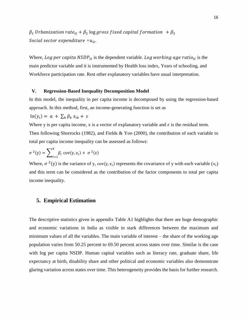
V. Regression-Based Inequality Decomposition Model
In this model, the inequality in per capita income is decomposed by using the regression-based
approach. In this method, first, an income-generating function is set as
ln(𝑦𝑖) = α + ∑ 𝛽𝑘 𝑥𝑖𝑘 + 𝜀𝑘
Where y is per capita income, x is a vector of explanatory variable and 𝜀 is the residual term.
Then following Shorrocks (1982), and Fields & Yoo (2000), the contribution of each variable to
total per capita income inequality can be assessed as follows:
𝜎 2(y) = ∑ 𝛽𝑖
𝑘
𝑖=1cov(y, 𝑥𝑖) + 𝜎 2(ε)
Where, 𝜎 2(y) is the variance of y, cov(y, 𝑥𝑖) represents the covariance of y with each variable (𝑥𝑖)
and this term can be considered as the contribution of the factor components to total per capita
income inequality.
5. Empirical Estimation
The descriptive statistics given in appendix Table A1 highlights that there are huge demographic
and economic variations in India as visible in stark differences between the maximum and
minimum values of all the variables. The main variable of interest – the share of the working age
population varies from 50.25 percent to 69.50 percent across states over time. Similar is the case
with log per capita NSDP. Human capital variables such as literacy rate, graduate share, life
expectancy at birth, disability share and other political and economic variables also demonstrate
glaring variation across states over time. This heterogeneity provides the basis for further research.
Page 17
17
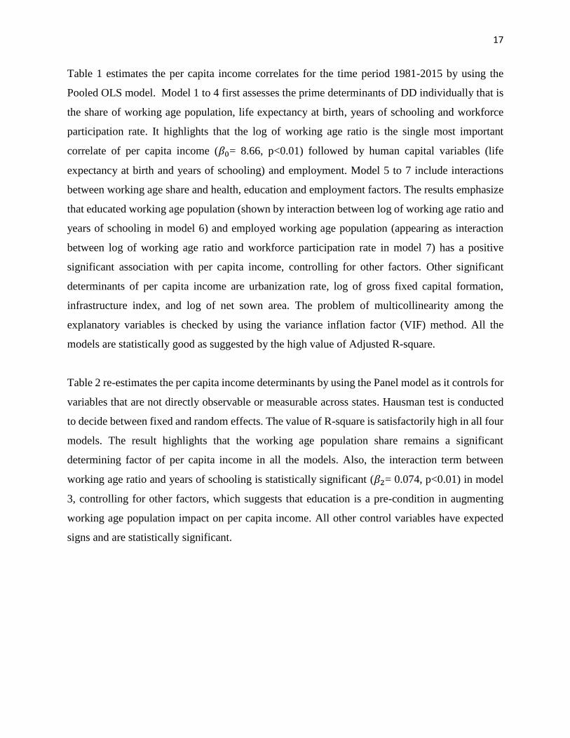
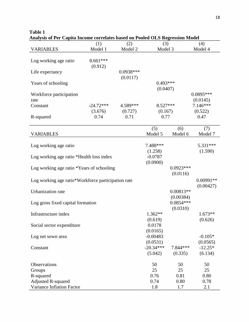
Table 1 estimates the per capita income correlates for the time period 1981-2015 by using the
Pooled OLS model. Model 1 to 4 first assesses the prime determinants of DD individually that is
the share of working age population, life expectancy at birth, years of schooling and workforce
participation rate. It highlights that the log of working age ratio is the single most important
correlate of per capita income (𝛽0= 8.66, p<0.01) followed by human capital variables (life
expectancy at birth and years of schooling) and employment. Model 5 to 7 include interactions
between working age share and health, education and employment factors. The results emphasize
that educated working age population (shown by interaction between log of working age ratio and
years of schooling in model 6) and employed working age population (appearing as interaction
between log of working age ratio and workforce participation rate in model 7) has a positive
significant association with per capita income, controlling for other factors. Other significant
determinants of per capita income are urbanization rate, log of gross fixed capital formation,
infrastructure index, and log of net sown area. The problem of multicollinearity among the
explanatory variables is checked by using the variance inflation factor (VIF) method. All the
models are statistically good as suggested by the high value of Adjusted R-square.
Table 2 re-estimates the per capita income determinants by using the Panel model as it controls for
variables that are not directly observable or measurable across states. Hausman test is conducted
to decide between fixed and random effects. The value of R-square is satisfactorily high in all four
models. The result highlights that the working age population share remains a significant
determining factor of per capita income in all the models. Also, the interaction term between
working age ratio and years of schooling is statistically significant (𝛽2= 0.074, p<0.01) in model
3, controlling for other factors, which suggests that education is a pre-condition in augmenting
working age population impact on per capita income. All other control variables have expected
signs and are statistically significant.
Page 18
18
Table 1
Analysis of Per Capita Income correlates based on Pooled OLS Regression Model
(1) (2) (3) (4)
VARIABLES Model 1 Model 2 Model 3 Model 4
Log working age ratio 8.661***
(0.912)
Life expectancy 0.0938***
(0.0117)
Years of schooling 0.493***
(0.0407)
Workforce participation
rate
0.0895***
(0.0145)
Constant -24.72*** 4.589*** 8.527*** 7.146***
(3.676) (0.727) (0.167) (0.522)
R-squared 0.74 0.71 0.77 0.47
(5) (6) (7)
VARIABLES Model 5 Model 6 Model 7
Log working age ratio 7.488*** 5.331***
(1.258) (1.590)
Log working age ratio *Health loss index -0.0787
(0.0900)
Log working age ratio *Years of schooling 0.0923***
(0.0116)
Log working age ratio*Workforce participation rate 0.00991**
(0.00427)
Urbanization rate 0.00813**
(0.00384)
Log gross fixed capital formation 0.0854***
(0.0310)
Infrastructure index 1.362** 1.673**
(0.619) (0.626)
Social sector expenditure 0.0178
(0.0165)
Log net sown area -0.00483 -0.105*
(0.0531) (0.0565)
Constant -20.34*** 7.844*** -12.25*
(5.042) (0.335) (6.134)
Observations 50 50 50
Groups 25 25 25
R-squared 0.76 0.81 0.80
Adjusted R-squared 0.74 0.80 0.78
Variance Inflation Factor 1.8 1.7 2.1
Page 19
19
Dependent variable is log per capita Net State Domestic Product. Robust standard errors in parentheses.
*** p<0.01, ** p<0.05, * p<0.1. Population adjusted weighted regression. In model 6, the individual
impact of log of working age ratio is not considered due to high pair wise correlation between log of
working age ratio and years of schooling.
Table 2
The Impact of Demography on Per Capita Income based on Panel Data Regression Model
(1) (2) (3) (4)
VARIABLES Random Effects
Model
Random Effects
Model
Fixed Effects
Model
Random Effects
Model
Log working age ratio 5.169*** 6.851*** 5.260***
(1.382) (1.202) (1.555)
Log working age
ratio*Health loss index
-0.109
(0.0904)
Log working age
ratio*Years of schooling
0.0743***
(0.0111)
Log working age
ratio*Work force
participation rate
0.00287
(0.00281)
Health loss index -1.409***
(0.467)
Urbanization rate 0.0176*** 0.0316** 0.00776*
(0.00646) (0.0134) (0.00434)
Log gross fixed capital
formation
0.119**
(0.0546)
Infrastructure index 1.570***
(0.588)
Credit/deposit ratio 0.00508 0.00305
(0.00465) (0.00582)
Social sector expenditure 0.0290*** 0.0210** 0.0291***
(0.00806) (0.00852) (0.00766)
Log net sown area -0.00488 -0.0302 -0.284* -0.164**
(0.0539) (0.0464) (0.138) (0.0741)
Constant -11.52** -17.45*** 10.66*** -11.27*
(5.380) (4.820) (1.074) (6.086)
Observations 50 50 50 50
Groups 25 25 25 25
R-square 0.75 0.72 0.77 0.75 Dependent variable is log per capita Net State Domestic Product. Robust standard errors in parentheses
*** p<0.01, ** p<0.05, * p<0.1. In model 3, the individual impact of log of working age ratio is not
considered due to high pair wise correlation between log of working age ratio and years of schooling
Page 20
20
Next, the results from the Conditional Barro Convergence model (Table 3) bring out the positive,
statistically significant and large impact of demographic factor - the initial share of working age
population and its growth over the period (1981-2011) on the per capita income growth (1981 –
2015). In model 1, an increase of one percent in the growth rate of working age ratio is associated
with an increase of 1.63 percent in average annual per capita income growth (𝛽1= 1.63, p<0.05)
and a one percent rise in the initial working age ratio leads to around seventeen percent rise in per
capita income growth over the period (𝛽0= 17.88, p<0.01). The sign of log of initial per capita
income is negative but not significant, suggesting weak convergence across states. Then in models
2 to 5, the robustness of demographic factors is checked by controlling core policy variables. The
model's explanatory power improve significantly with adjusted R-square reaching 65 percent. In
model 5, when all socio-economic factors are controlled, the point estimate of the growth rate of
the working age ratio is still quantitatively stable and has a significant impact on per capita income
growth (𝛽1 = 1.05, p<0.05). The coefficient of the initial working age ratio reduces substantially
in magnitude (𝛽0= 9.54, p<0.05) after controlling other factors. Further, among the core policy
variables, only the credit – deposit ratio is having a significantly positive impact on per capita
income growth.2
In Table 4 the estimates of the Conditional Barro regression model are extended to include the
interaction effect of age structure variable with initial health factor, initial education factor, and
initial workforce participation rate. The models are a good fit as suggested by the high value of
Adjusted R-square. The results bring to notice the importance of health and employment in
realizing DD. It indicates that the impact of the increase in working age share on per capita growth
is reduced significantly (𝛽0 = - 0.69, p<0.01) when the working age suffers from health burden
(captured by the interaction between growth in working age share and health loss index in model
1), controlling for other factors. Similarly, in model 3 the impact of the increase in working age
2 The existing literature argues that there is a contemporaneous relation between per capita income growth and working age population growth due to the migration effect. People of working age tend to migrate to regions experiencing better economic development and thereby leading to higher growth in the working age population in that region. However, the inter-state migration in India has been found to be less responsive to per capita income differences due to the presence of resistance from local labour unions, strong linguistic and cultural barriers and paucity of urban shelter for migrants (Cashin & Sahay, 1996; Datta, 1985; Skeldon, 1986; Aiyar & Mody, 2011). Also, the data on migration for the period 2011 from the Census of India was not available at the time of writing this paper. So the growth rate in the working age population could not be adjusted for migration effect.
Page 21
21
share gets enhanced when working age people are employed (𝛽2 = 0.015, p<0.05), controlling for
other factors.
Table 3
Estimates of Demographic Dividend from Conditional Barro Convergence Regression
Model
(1) (2) (3) (4) (5)
VARIABLES Model 1 Model 2 Model 3 Model 4 Model 5
Log initial working
age ratio
17.88*** 17.99*** 13.95*** 9.357** 9.537**
(3.826) (3.936) (4.668) (4.295) (4.485)
Growth in working
age ratio
1.630** 1.402** 2.290** 1.210** 1.054**
(0.773) (0.603) (0.804) (0.465) (0.445)
Log initial per capita
income
-0.195 -0.0781 -0.0370 -0.257 -0.215
(0.493) (0.398) (0.383) (0.283) (0.253)
Disability share -3.930* -2.024
(1.967) (1.478)
Graduate share -0.187 -0.00213
(0.109) (0.115)
Urbanization rate 0.0169
(0.0230)
Governance index 0.124*
(0.0703)
Infrastructure index 0.645
(1.504)
Credit/deposit ratio 0.0341*** 0.0307**
(0.0114) (0.0116)
Constant -71.89*** -71.60*** -61.54*** -37.85** -37.62*
(13.82) (15.95) (19.26) (17.43) (18.18)
Observations 50 50 50 50 50
Groups 25 25 25 25 25
R-squared 0.55 0.63 0.64 0.72 0.74
Adjusted R-squared 0.48 0.53 0.54 0.64 0.65
Variance inflation
factor
1.2 1.3 1.6 1.5 1.7
Dependent variable is growth in per capita net state domestic product (1981 – 2015). Robust standard errors
in parentheses. *** p<0.01, ** p<0.05, * p<0.1. Population adjusted weighted regression. All control
variables are measured at initial time period (1981).
Page 22
22
Table 4
Impact of the Interaction of Demography with the Key Policy Variables on Per Capita
Growth in Conditional Barro Convergence Regression Model
(1) (2) (3)
VARIABLES Model 1 Model 2 Model 3
Growth in working age ratio*Health-loss
index
-0.699***
(0.243)
Growth in working age ratio*Literacy rate 0.00520
(0.00368)
Growth in working age ratio*Workforce
participation rate
0.0152**
(0.00611)
Log initial working age ratio 7.234* 10.74*** 10.10**
(3.531) (3.694) (4.270)
Log initial per capita income 0.295 0.422 -0.498
(0.280) (0.284) (0.403)
Health-loss index -2.324**
(0.887)
Log gross fixed capital formation 0.481*** 0.489***
(0.121) (0.155)
Infrastructure index 0.892
(1.516)
Social sector expenditure 0.155** 0.195**
(0.0709) (0.0806)
Constant -32.15** -49.80*** -32.67*
(14.89) (14.08) (17.82)
Observations 50 50 50
Groups 25 25 25
R-squared 0.70 0.62 0.66
Adjusted R-squared 0.62 0.52 0.57
Variance inflation factor 1.8 1.9 1.5
Dependent variable is growth in per capita net state domestic product (1981 – 2015). Robust standard errors
in parentheses. *** p<0.01, ** p<0.05, * p<0.1. Population adjusted weighted regression. All control
variables are measured at initial time period (1981)
Page 23
23
Table 5 presents an alternative approach of figuring out the influence of working age share on per
capita income by using health loss index, years of schooling and workforce participation rate as
instruments for the working age share. The Two-Stage Least Square (2SLS) estimates highlight
the statistical significant bearing of working age share on per capita income (𝛽0 = 7.99 p<0.01),
controlling for other factors. The instruments used are valid as per the test of over-identifying
restrictions and the value of F-statistic shows that instruments are not weekly correlated with the
endogenous regressors. Also, under the endogeneity test, the null hypothesis of the exogeneity of
the working age share is rejected at a conventional level of significance. Therefore, this model
reassures that the working age population works through the channels of quality education, good
health, and decent employment opportunities to promote economic growth.
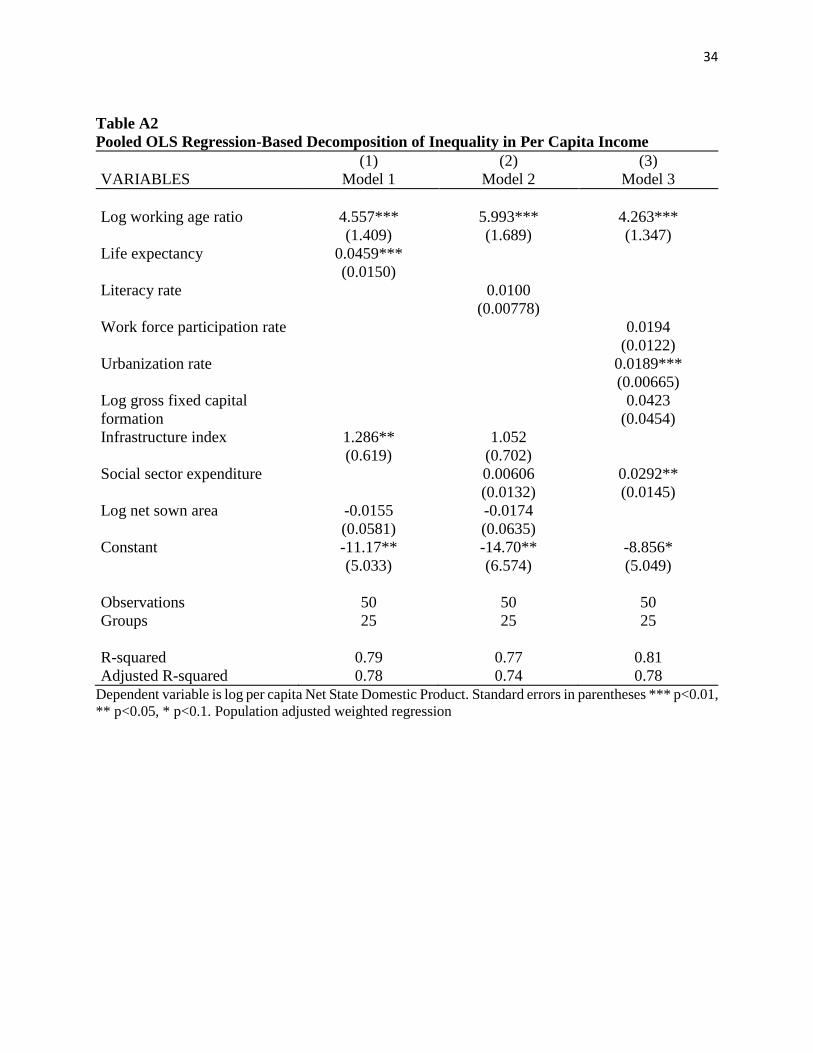
Next, the relative contribution of the working age population in explaining per capita income
inequality across states over the period (1981 – 2015) is computed based on the Regression-Based
Inequality Decomposition Model. In this method, three different models of pooled OLS regression
are run based on the correlation among the explanatory variables (given in Appendix Table A2).
Based on these regression results, Table 6 highlights that the maximum portion of per capita
income inequality is attributable to divergent share of the working age population across states.
Around 37 percent to 52 percent of income inequality is contributed by working age share across
states, once we control for other core economic variables. The next important variable significantly
contributing to inequality is the health factor captured by the life expectancy rate (around 35
percent). Besides this, the varying rate of urbanization across states also significantly causes
income inequality (around 20 percent), followed by social sector expenditure (around 9 percent)
and availability of infrastructure (6 percent). Surprisingly, the relative contribution of literacy rate
and employment to explain income inequality do not turn out to be significant, possibly pointing
towards their poor quality. Around 20 percent of the income inequality is still unexplained as
suggested by the residual term.
Page 24
24
Table 5
Impact of Demography on Per Capita Income through Instrumental Variables Model
VARIABLES 2SLS
Log working age ratio 7.992***
(1.735)
Urbanization rate 0.00889
(0.00627)
Log gross fixed capital formation 0.0244
(0.0305)
Social sector expenditure 0.00918
(0.0142)
Constant -22.60***
(6.659)
Observations 50
Groups 25
R-squared 0.77
Dependent variable is log per capita NSDP
Robust Standard errors in parentheses. *** p<0.01, ** p<0.05, * p<0.1.
Population adjusted weighted regression
Instrumented: Log working age ratio
Instruments: Health loss index, Years of schooling, Workforce participation rate
First stage F statistic 23.38
Over-identifying Restrictions
Ho: zero correlation between instruments and the error term
Sargan chi2(2) = 2.05555 (p = 0.3578)
Basmann chi2(2) = 1.84357 (p = 0.3978)
Score chi2(2) = 2.13991 (p = 0.3430)
Exogeneity of instrumented explanatory variable H0: Variable is exogenous
Robust score chi2(1) = 8.60546 (p = 0.0034)
Robust regression F(1,44) = 8.66364 (p = 0.0052)
Page 25
25
Table 6
Contribution of Demography to Inter-State Inequality in Per Capita Income
(1) (2) (3)
VARIABLES Model 1 Model 2 Model 3
Log working age ratio 39.01*** 51.29*** 36.48***
Life expectancy 34.77***
Literacy rate 18.60
Work force participation rate 10.21
Urbanization rate 19.58***
Log gross fixed capital formation 5.28
Infrastructure index 5.70** 4.66
Social sector expenditure 1.92 9.22**
Log net sown area 0.41 0.45
Residual 20.10 23.05 19.19
Total 100 100 100
Dependent variable is log per capita Net State Domestic Product. Standard errors in parentheses *** p<0.01,
** p<0.05, * p<0.1. Population adjusted weighted regression. The Pooled OLS Regression of
Decomposition model is given in Appendix Table A2.
6. Challenges in the way of realizing Demographic Dividend
Given the fact that the window of DD has just started in 2018 and will continue till 2055, the
current demographic transition has not been accompanied by requisite socio-economic changes
which pose some of the serious growth constraints mentioned below:
First, the public investments in social infrastructure in India are abysmal. The total expenditure on
health as a percentage of GDP is scarcely 1.5 percent while the global average is around 6 percent.
This meager budgetary allocation on health has resulted in escalating out-of-pocket expenditure of
people. Although there is tremendous improvement in health indicators like Maternal Mortality
Rate, Infant Mortality Rate, Under-five Mortality Rate, Life Expectancy at Birth over the past few
years, yet due to prevalence of chronic illnesses and disabilities, the diseases adjusted life
expectancy in India is only 53.5 years (Goli & Pandey, 2010; James & Goli, 2016). Further, there
is a disparity in health infrastructure in rural areas which has led to inter-state variations in health
indicators. For instance, as per the Economic Survey (2018 – 19), states with shortfalls of doctors
and specialists have higher rural IMR and MMR as compared to other states. Thus, the goals of
Page 26
26
accessible, affordable and quality health care require adequate infrastructure facilities, proper
monitoring of the staff, and provision of essential supplies. On the education front, the government
spending on education as a percent of GDP is merely 3 percent in 2018 – 19 (Economic Survey
2018 – 19). Though there is remarkable progress in India’s Gross Enrolment Ratio (GER) in the
primary and secondary level, it is significantly lower in higher education (25.8 percent in 2017-18
as per MHRD provisional data). Also, there is a disparity in higher education levels across gender
and backward social groups (Educational Statistics at a Glance 2018 cited in Economic Survey
2018 – 19). The literacy rate has touched 77 percent mark in 2017 – 18 (PLFS Annual report 2017-
18), but the learning outcomes are still miserable. The Annual Status of Education Report (2018)
cited in Economic Survey (2018 – 19) highlights that 1 out of 4 children leaving class VIII lack
basic reading skills. The quality of the workforce depicted by its skill profile is also gloomy. As
per the Periodic Labour Force Survey (PLFS) Annual Report (2017 – 18), the proportion of urban
youth who received formal vocational training was only 4.4 percent in 2017 – 18. It seems to be a
formidable task of training 400 million people by 2022 as per the target of the Ministry of Skill
Development and Entrepreneurship.
Second, the generation of gainful and quality employment opportunities at a fast pace is essential
in India provided the fact that 63 percent of the population is in the working age group. However,
as per the PLFS Annual Report (2017 – 18), around half of the working age population in India is
out of the labor market. The Labour Force Participation Rate (LFPR) in usual status has declined
from 55.9 percent in 2011 – 12 to 49.8 percent in 2017 – 18. Further, there is a worsening of the
quality of employment due to the growing informalization and casualization of jobs. One cannot
ignore the other half of DD that is the status of women in the sphere of education, health, and labor
market. The LFPR of women has declined twice as compared to their counterparts from 2011 – 12
to 2017 – 18 and less than a quarter of them are active in the labor market in 2017 – 18. Though
urban women LFPR has remained stagnant at 20.4 percent from 2011 – 12 to 2017 – 18, it has
declined sharply by 11 percentage points for rural females during the same period. Thus, the female
LFPR in India is one of the lowest in the world. Further, it is found that there exist huge gender
disparities in education, health, marriage, and the overall sex ratio which if removed could
contribute an additional $2.9 trillion in real terms by 2025 (Dobbs et al., 2015). Also, there is a
huge prevalence of child marriages in India. According to Goli (2016) estimates, the number of
Page 27
27
child marriage in India (103 million) is greater than the population of the Philippines and out of
28 child marriages taking place per minute across the world, more than two of them are held in
India. This has a significant negative effect on health and needs to be controlled to prevent its
adverse effects on the economy.
The next upcoming issue emerging from the age structure transition of the population is the rapidly
growing old-age dependency ratio in the future. According to Goli and Pandey (2010) estimates
from UN projections, there will be only a 2 percent increase in the working age population between
2005 – 2050 whereas the older population will go up by 13 percent during the same period. Also,
in India, it takes only 25 years to double its older population as compared to the US where it takes
around 70 years for the same. Thus, India will prematurely develop into aging societies which will
have serious economic and health burdens. But this may provide the possibility of the ‘Second
Demographic Dividend’ as the older population aids in capital accumulation from the savings done
during their working years and thereby leading to economic growth. However, it hinges on the
availability of developed financial markets, healthy older population, provision of income security
and social security, which at present seems to be an arduous task in India. Therefore, India should
start preparing for this future challenge otherwise it may get old before getting rich.
The fourth constraint is the negative trend in household savings rate which is a principal source of
capital accumulation and an important parameter of DD. It has fallen from 23.6 percent in 2011 –
12 to 17.2 percent in 2017 – 18 which has put a drag on investment rate by almost 10 percentage
points during this period. Besides this, according to Oxfam India Report (2018), India has the
highest disparity among all the nations the world on all the parameters of income, wealth and
consumption. This rising income disparity may further dampen the savings rate in the future.
Lastly, the level of urbanization in India is around 34 percent in 2018 as per the report of U.N.
World Urbanization Prospects (2018). But there is a vast interstate disparity in its level ranging
from 10 percent in Himachal Pradesh to 48.5 percent in Tamil Nadu. As cities attract working age
people in search of better employment opportunities and livelihood, this promotes inter-state
migration and accentuate already existing economic inequalities in India. As per Census 2011, the
population growth in urban areas has been contributed more by migration than the natural
Page 28
28
population growth. Also, this rapid pace of urbanization without advancement in rural areas has
put excessive population pressure in cities and simultaneously leading to urbanization of rural
poverty. In such a scenario, it is essential to co-develop both urban and rural areas to maintain
balance and equip the youth with quality education, skills and decent employment opportunities
(James & Goli, 2016).
7. Conclusion
The analysis based on the panel of 25 states of India has reckoned DD to be about one percentage
points per annum for the period 1981 – 2015, after controlling core policy variables. The results
suggest that the economic convergence of states could be achieved if the working age population
is healthy, educated, and employed. Also, the working age population has emerged out as a major
factor contributing to per capita income inequality across states. But this common conclusion about
India needs to be qualified in the light of the fact of huge inter-state variations in socio-economic
and demographic profiles. The realization of DD is conditional on the performance of northern
states where the population bulge or the window of opportunity has just begun but these states
typically underperform as compared to other Indian states. Some other major lacunas in reaping
the desired benefits of demographic change is dwindling spending on education and health sector;
low adult literacy rate; skill mismatches; presence of chronic illnesses and disabilities; falling
employment rates; gender disparities in education, health, labor market, and overall sex ratio; child
marriage; falling household savings rate; urbanization of rural poverty; and rapidly rising aging
population in future. Therefore, given India’s high levels of internal heterogeneity, prompt policy
action to ameliorate these challenges is crucial to prevent DD to turn in to a demographic burden.
Page 29
29
References
Acharya, S. (2004). India’s Growth Prospects Revisited. Economic and Political Weekly, 39(41),
1515–1538
Aiyar, S. & Modi, A. (2011). The Demographic Dividend: Evidence from Indian States. IMF
Working Paper 11/38. Retrieved from https://www.imf.org/external/pubs/ft/wp/2011/wp1138.pdf.
Birdsall, N., Kelley, A. C., & Sinding, S. (2003). Population Matters: Demographic Change,
Economic Growth, and Poverty in the Developing World. Oxford Scholarship Online. ISBN-13:
9780199244072. DOI:10.1093/0199244073.001.0001
Bloom, D.E. & Freeman, R.B. (1988). Economic development and the timing and components of
population growth. Journal of Policy Modeling, 10(1), 57-81.
Bloom, D.E. & Sachs, J.D. (1998). Geography, demography, and economic growth in Africa, In
Brainard, W.C. and Perry, G.L. (Eds.), Brookings Papers on Economic Activity, 2, 207-295.
Bloom, D. E. & Williamson, J. G. (1998). Demographic Transitions an Economic Miracles in
Emerging Asia. World Bank Economic Review, 12(3), 419-56.
Bloom, D. E., Canning, D., & Malaney, P., (2000). Population dynamics and economic growth in
Asia. Population and Development Review, 26, 257–290.
Bloom, D.E., Canning, D., & Sevilla, J. (2001). Economic growth and the demographic transition,
NBER Working Papers 8714, National Bureau of Economic Research, Inc.
Bloom, D. E., Canning, D. & Sevilla, J. (2003). The demographic dividend: A new perspective on
the economic consequences of population change. Santa Monica, CA: Rand.
Bloom, D. E. & Canning, D. (2004). Global Demographic Change: Dimensions and Economic
Significance. NBER Working Paper 10817, NBER.
Bloom, D. E. & Finlay, J. E. (2008). Demographic Change and Economic Growth in Asia. Program
on the Global Demography of Aging Working Paper 41, PGDA Retrieved from: http://www.hsph.harvard.edu/pgda/working.htm
Bloom, D. E. (2011). Population Dynamics in India and Implications for Economic Growth.
PGDA Working Paper No.65. Retrieved from http://www.hsph.harvard.edu/program-on-the-global-
demography-of-aging/WorkingPapers/2011/PGDA_WP_65.pdf.
Cashin, P. & Sahay, R. (1996). Internal Migration, Center-State Grants and Economic Growth in
the States of India. IMF Staff Papers, 43(1).
Census. (1981, 2011). Office of Registrar General, Ministry of Home Affairs, Government of
India.
Page 30
30
Chandrasekhar, C.P., Ghosh, J., & Roychwdhury, A. (2006). The Demographic Dividend and
Young India’s Economic Future. Economic and Political Weekly, 41(49), 5055-5064.
Coale, Ashley J. & Hoover, E. (1958). Population growth and Economic Development in low
Income Countries – A Case Study of India’s Prospects. Princeton: Princeton University Press.
Datta, P. (1985). Inter State Migration in India. Margin, 18(1), 69-82.
Desai, S. (2010). The Other Half of the Demographic Dividend. Economic & Political Weekly,
14(40), 12–14.
Dobbs, R., Manyikaet, J., & Woetzel, J. (2015). The Power of Parity: Advancing Women’s
Equality in India. McKinsey Global Institute.
Fields, G., & Yoo, G. (2000). Falling labour income inequality in Korea’s economic growth:
patterns and underlying causes. Review of Income Wealth, 46(2), 139–159.
Goli, S. & Pandey, A. (2010). Is India ‘getting older before getting rich’? Beyond demographic
assessment. Research Gate, Retrieved from: https://www.researchgate.net/publication/234040176
Goswami, B. & Bezbaruah, M. P. (2011). Social Sector Expenditures and Their Impact on Human
Development: The Indian Experience. Indian Journal of Human Development, 5(2).
Higgins, M. & Williamson, J.G. (1997). Age structure dynamics in Asia and dependence of foreign
capital. Population and Development Review, 23(2), 261-293.
James, K. S. (2008). Glorifying Malthus: Current Debate on ‘Demographic Dividend’ in India.
Economic & Political Weekly, 43(25), 63-69.
James, K. S. (2011). India's Demographic Change: Opportunities and Challenge. Science, 333,
576, DOI: 10.1126/science.1207969
James, K. S. & Goli, S. (2016). Demographic Changes in India: Is the Country Prepared for the
Challenge. Brown Journal of World Affairs, 23(1), 169–187.
Joe, W., Kumar, A., & Rajpal, S. (2018). Swimming against the tide: economic growth and
demographic dividend in India. Asian Population Studies, DOI: 10.1080/17441730.2018.1446379
Kumar, U. (2013). India’s Demographic Transition: Boon or Bane?. Asia and the Pacific Policy
Studies, 1(1), 186–203.
Ladusingh, L. & Narayana, M. R. (2011). Demographic Dividends for India: Evidence and
Implications Based on National Transfer Accounts. ADB Economics Working Paper Series 292.
Lee, R. & Mason, A. (2006). Back to Basics: What is the Demographic Dividend. Finance &
Development, 43(3), 16-17.
Mason, A. (2001). Population Change and Economic Development in East Asia: Challenges
Page 31
31
Met, Opportunities Seized. Stanford, Stanford University Press.
Mason, A. (2005). Demographic Transition and Demographic Dividends in Developed and
Developing Countries. United Nations Expert Group Meeting on Social and Economic
Implications of Changing Population Age Structure, Mexico City, August 31-September 2.
Ministry of Skill Development & Entrepreneurship, Government of India. (2015). National Policy
for Skill Development and Entrepreneurship Report. Retrieved from: Http://Pibphoto.Nic.In/Documents/Rlink/2015/Jul/P201571503.Pdf
Ministry of Finance, Government of India. (2019). Economic Survey 2018 – 19. Retrieved from: https://www.indiabudget.gov.in/economicsurvey/
Ministry of Statistics and Programme Implementation, Government of India. (2019). Periodic
Labour Force Survey (PLFS) Annual Report (2017 –2018). Retrieved from: http://mospi.nic.in/sites/default/files/publication_reports/Annual%20Report%2C%20PLFS%202017-
18_31052019.pdf?download=1
Mitra, S. & Nagarajan, R. (2005). Making Use of the Window of Demographic Opportunity: an
Economic Perspective. Economic and Political Weekly, 40(50), 5327–32.
Navaneetham, K. (2002). Age Structural Transition and Economic Growth: Evidence from South
and Southeast Asia. Centre for Development Studies Working Paper No 337, Retrieved from: http://unpan1.un.org/intradoc/groups/public/documents/apcity/unpan012698.pdf
Oxfam India Report. (2018). Mind the Gap - The State of Employment in India. Retrieved from: https://www.oxfamindia.org/sites/default/files/2019-03/Full%20Report%20-%20Low-
Res%20Version%20%28Single%20Pages%29.pdf
Reserve Bank of India. (2018). Handbook of Statistics on Indian States. Retrieved from: https://rbidocs.rbi.org.in/rdocs/Publications/PDFs/0HANDBOOK201819_FDF254115C6094E3CAB32A
1DCDA9ADA88.PDF
Shorrocks, A. F. (1982). Inequality decomposition by factor components. Econometrica, 50(1),
193–211.
Skeldon, R. (1986). Migration Pattern in India during the 1970s. Population and Development
Review, 12(4), 759-780
Thakur, V. (2012). The Demographic Dividend in India: Gift or curse? A State level analysis on
differing age structure and its implications for India’s economic growth prospects. International
development, London School of Economics and Political Science, Working Paper- No.12-128.
Thompson, W. S. (1929). Population. American Journal of Sociology, 34(6), 959-975.
United Nations, World Population Prospects: The 2019 Revision. Department of Economic and
Social Affairs, Population Division, New York.
Page 32
32
United Nations, World Urbanization Prospects: The 2019 Revision. Department of Economic and
Social Affairs, Population Division, New York. Retrieved from:
https://population.un.org/wup/Publications/Files/WUP2018-Report.pdf
UNFPA (2019). Demographic Dividend Opportunity in India: Evidence and Policy Imperatives.
Unpublished document.
Page 33
33
APPENDIX
Table A1
Data Source and Descriptive Statistics of the Variables
Variables Data source Mean Std.
Dev.
Min. Max.
Outcome
variable
Log net state
domestic product
Central Statistics
Organization
10.7 0.9 9.1 12.5
Predictor variable
Demographic
factor
Working age
ratio (%)
Census of India 1981 and
2011
58.9 4.99 50.25 69.50
Covariates
Social
factors
Literacy rate Census of India 60.4 19.9 24.2 94.0
Graduate share NSSO employment–
unemployment round 4.4 3.7 0.7 19.5
Years of schooling NSSO employment–
unemployment round 4.3 1.6 1.7 7.6
Disability share Census 1981 and 2011 1.2 1.0 0.1 3.0
Life expectancy at
birth
Sample Registration
System 64.0 7.4 50.0 75.0
Health loss index Constructed from
weighted average of
disability share, life loss
and infant mortality rate. 0.5 0.2 0.1 0.9
Political
factors
Urbanization rate Census of India 28.3 17.9 6.6 97.5 Governance index Basu (2002) 5.0 2.9 0.0 10.0
Economic
factors
Infrastructure
index (Based on
Road density,
Electricity
consumption, Rail
Route length, and
Post Office)
Report of Tenth Five Year
Plan and RBI handbook of
state statistics.
0.2 0.1 0.0 0.8
Credit – deposit
ratio
Statistical Tables Relating
to Banks, RBI 54.7 25.6 6.2 116.2
Log Gross fixed
capital formation
RBI handbook of state
statistics 8.8 2.8 0.3 13.5
Workforce
Participation Rate
Census of India 38.1 6.8 26.7 51.8
Log Net sown area
(thousand
hectares)
M/o agriculture and
farmer’s welfare and RBI
handbook of state statistics 7.4 1.9 3.1 9.9
Social sector
expenditure (as a
% of GSDP)
Goswami and Bezbaruah
(2011) and RBI handbook
of state statistics 13.1 9.5 1.6 52.8
Page 34
34
Table A2
Pooled OLS Regression-Based Decomposition of Inequality in Per Capita Income
(1) (2) (3)
VARIABLES Model 1 Model 2 Model 3
Log working age ratio 4.557*** 5.993*** 4.263***
(1.409) (1.689) (1.347)
Life expectancy 0.0459***
(0.0150)
Literacy rate 0.0100
(0.00778)
Work force participation rate 0.0194
(0.0122)
Urbanization rate 0.0189***
(0.00665)
Log gross fixed capital
formation
0.0423
(0.0454)
Infrastructure index 1.286** 1.052
(0.619) (0.702)
Social sector expenditure 0.00606 0.0292**
(0.0132) (0.0145)
Log net sown area -0.0155 -0.0174
(0.0581) (0.0635)
Constant -11.17** -14.70** -8.856*
(5.033) (6.574) (5.049)
Observations 50 50 50
Groups 25 25 25
R-squared 0.79 0.77 0.81
Adjusted R-squared 0.78 0.74 0.78
Dependent variable is log per capita Net State Domestic Product. Standard errors in parentheses *** p<0.01,
** p<0.05, * p<0.1. Population adjusted weighted regression