DENSE-PHASE PNEUMATIC TRANSPORT OF COHESIONLESS SOLIDS by Thomas s . Totah Thesis submitted to the Faculty of the Virginia Polytechnic Instib.Jte and state University in partial fulfillment of the requirements for the degree of MASTER OF SCIENCE in Chemical Engineering APPROVED: Dr • Kenneth Konrad, Chairman Dr. Arthur M. Sqll(Lres Dr. John c. Parker July, 1987 Blacksburg, Virginia
Transcript
DENSE-PHASE PNEUMATIC TRANSPORT OF COHESIONLESS SOLIDS
by
Thomas s . Totah
Thesis submitted to the Faculty of the
Virginia Polytechnic Instib.Jte and state University
in partial fulfillment of the requirements for the degree of
MASTER OF SCIENCE
in
Chemical Engineering
APPROVED:
Dr • Kenneth Konrad, Chairman
Dr. Arthur M. Sqll(Lres Dr. John c. Parker
July, 1987
Blacksburg, Virginia
DENSE-PHASE PNEUMATIC TRANSPORT OF COHESIONLESS SOLIDS
by
Thomas s . Totah
Committee Chairman: Dr . .Kenneth .Konrad Department of Chemical Engineering
(ABSTRACT)
An experimental program has been undertaken to gain a more fundamental
understanding of dense-phase pneumatic transport of cohesionless solids. A
50. a mm internal diameter circulating unit with both horizontal and vertical
sections has been constructed . The pipe material is transparent lexan which
allows for visual observation of the flow pattern. The particles used were a
mixture of 95'% white and 5~ black polyethylene granules (particle diameter
approximately 3 mm) . The black particles were used to aid the visual
observation of the flow pattern. The flow patterns ranged from dilute-phase
flow to dense-phase plug flow. High-speed photographic techniques have been
used to document the flow patterns in both the horizontal and vertical sections.
Pressure drop measurements across a 70 cm test section have been coordinated
with the film work.
At the higher superficial air velocities (approximately 15 m/sec), the
particles flow in a dilute suspension within the air stream . The pressure drop
across the 70 cm section fluctuates very rapidly . For the horizontal
dilute-phase flow, the mean pressure drop is approximately 0.12 kPa with
fluctuations ranging from O to o • 3 kPa. For the vertical dilute-phase flow, the
mean pressure drop is approximately o. 25 kPa with fluctuations ranging from O
to o. 5 kPa. CJpon reducing the superficial air velocity to 6. 8 m/sec, the flow
pattern in the horizontal section changes to a type of strand flow. The
particles are conveyed in a dilute phase above a stationary layer. Large peaks
in the pressure drop data (approximately 1 to 2 kPa) correspond to increases
in the dilute-phase solids concentration.
At the lower superficial air velocities (below 5 m/sec) , the solids flow
pattern changes to dense-phase flow. The particles move in the form of plugs
that occupy the entire pipe cross-section. For the horizontal flow, the plug
length ranged from o . 1 7 to o. 60 m and the pressure drop across the plugs
ranged from 1 to 5 • 2 kPa. The pressure gradient range can be predicted from
the equations of Konrad et al. ( 1980) . The analysis of the vertical
dense-phase flow films is not as straightforward as the horizontal films.
Bowever , the flow pattern resembles that described by Konrad ( 198 7 ) and there
is qualitative agreement with the concepts ouUined by Konrad (1987).
Acknowledgments
The list of people who have supported me as I worked toward the
completion of this thesis is very long indeed. First of all I thank my advisor ,
Dr . Kenneth Konrad , for his guidance and assistance in all aspects of this
work. I would also like to thank Dr. A. M • Squires and Dr. :r. c. Parker for
serving on my graduate advisory committee •
I am grateful to the National Science Foundation for their financial support
and to the Phillips 66 Company for supplying the polyethylene granules used in
the experiments •
The staff at Virginia Tech and many of my colleagues deserve recognition
for their contributions, especially:
Riley Chan for his many helpful suggestions and for his electronic wizardry.
Billy Williams and Wendell Brown for fabricating numerous items of equipment.
Mark Mason and Vance Bergeron for their assistance in assembling the circUlating unit.
The Virginia Tech film unit for their advice and the use of equipment.
Benku Thomas, Renato sprung , and c . w . Cheah for many rewarding discussions .
My fellow graduate students Greg Benge, Danny Thompson, Carl Reed, Jeff Smith, Paul Hathaway, and Alma Rodarte (among many others) for their continuous encouragement.
Finally , I thank my family for their unending love and support.
4.2 Wall Friction Shear stress Data ••.•••.••••••••.•••••.. 56
4.3 Summary of Particle Properties 60
4.4 Horizontal Conveying: operating Conditions for the Five Experimental Runs ••. 63
4.5 Horizontal Conveying: Summary of the Results Obtained from Dense-Phase Plow Film Work . . . • • . • • . • • • • • 77
4.6 Vertical Conveying: Operating Conditions for the Pour Experimental Runs ..• 83
xiii
List of Symbols
A Pipe cross -sectional area
Ast Settled streamer cross-sectional area
Be Ratio of compressive stresses in the plug (close to one for ideal plugs)
c Plug speed
c Interparticle cohesion
Cw Particle /wall cohesion
D Pipe diameter
dp Particle diameter
F Stress on plug front
Frc Froude number
g Acceleration due to gravity
Kw Coefficient of internal friction at the wall
Ip Plug length
R Radial distance from center of shear cell
Ri Inner radius of shear cell
Ro outer radius of shear cell
Sc Force due to collection of streamer
T Total shear torque
Ug Particle velocity within a plug
w An indicator of the fractional change in fluid pressure gradient with respect to the logarithm of the particulate normal stress
Wp Wave front velocity
xiv
Greek Symbols
6P Pressure drop across the plug
e Angle of pipe inclination
Ii Dimensionless measure of the plug length
11 Ratio of radial to axial compressive stress
µ. Coefficient of internal friction
µ._, Coefficient of wall friction
Pb Solids bulk density
Pb, st Solids bulk density in the settled streamer
a Normal stress
aw Normal stress for wall friction
-r Shear stress
T" w Wall shear stress
41 Angle of internal friction
41w Angle of wall friction
x Wedge number
~ Angle of wall friction
= (Note: strictly this is for cohesionless materials, but is a good approximation for cohesive materials) •
xv
1.0 INTRODUCTION
Many processes require the conveyance of bulk solids from one point to
another within the plant site. There are a variety of methods for moving solids
which can be divided into two broad categories: ( 1 ) mechanical conveying and
( 2) pneumatic conveying (refer to Figure 1. 1) . Since solid properties (bulk
density, particle size and shape, etc. ) vary greatly, each operation is unique.
Therefore, a transport system must be designed to meet a particular need,
taking into account such factors as the particle properties , conveying rates,
conveying distance and path, and the operating environment ( Reece, 1985) •
There are many different types of mechanical conveyors and elevators
( Colijn, 1981) . The movement in mechanical conveyors is horizontal or on an
incline from the horizontal ( -10 -15 °) , whereas that in elevators is vertical or
on an incline from the vertical (-15°). The most common types of conveyors
are belt, screw, chain and vibratory, and the most common elevators are
bucket, screw and vibratory • Basically , all of these devices utilize some kind
of mechanical motion (the movement of a belt, turning of a screw, raising of
buckets , etc . ) to transport the solids from one location to another •
Pneumatic conveying of solids , on the other hand , can be described as the
use of the energy of flowing air to move solids through a pipeline. The first
conveying line was set up in 1887 to transport agricultural products (Rizk,
1986). Since that time, pneumatic conveying has found applications in a wide
range of industries (cement, baking , plastics , pulp and paper , and synthetic
1
So 1 ids Hand! ing
l i
Pneumatic Conveying
i 1 ! N
1 Bell Screw Chain Vibratory Buckel• Vacuum Sy•leam Pr•••ur• Sy•l•m•
l 1
Di lute Ph••• Deu.e Pha••
Figure 1.1 Solids Handling Options Within a Plant Site
3
fuels to name a few). Pneumatic conveyors offer some advantages over
mechanical conveyors ( Stoess, 1983) . First, the straightline conveying of
mechanical conveyors is eliminated. Mechanical conveyors require transfer
points for changes in direction , therefore a series of conveyors may be
required which can add to the cost and to control problems. In pneumatic
conveying , short and long radius bends are utilized to change direction and to
bypass obstructions . Also , space and accm;ses needed for maintenance
purposes are minimized . A second advantage of pipeline conveying is
cleanliness . The solids transported by mechanical conveyors are open to the
atmosphere which can cause significant dust problems, especially at transfer
points. Since the solids are enclosed in a pipe in pneumatic conveying, the
dust problem is virtually eliminated. Also , there is little chance for
contamination of the solid product in a pneumatic conveying system. This is
important in the transport of foodstuffs , pharmaceuticals , or even plastics where
one different-colored part in 80, ooo may cause an off-color condition to the
final product ( stoess, 1983) . A third advantage of pneumatic conveyors is
greater safety over their mechanical counterparts. Fire and explosion hazards
are reduced . There is less risk of injury while conveying hazardous materials.
This enhanced safety factor can result in lower insurance rates for industries
that utilize pneumatic conveyors.
One of the prime disadvantages of pneumatic conveyors is that, even to this
day, the design of these systems is more of an art than a science. Each
year, researchers are learning more about the two-phase gas-solid flows
thereby improving the reliability, but the final design is primarily based on
4
experimental correlations, tests with the actual material to be conveyed and
past experience . Another disadvantage of pneumatic conveyors is the higher
power costs compared to other conveyors. Recent research has been aimed at
lowering this cost. A third disadvantage is the higher initial capital
investment, but this can be offset by the labor -saving quality and possible
reduction in insurance rates . A minor disadvantage is the ability of this
conveyor to convey in one direction only. There are some limitations to the
selection of pneumatic conveyors. These limiting factors are primarily based on
the characteristics of the material and the conveying distance . Reece (1985)
provides some general guidelines for deciding which type of system might be
best suited for a particular application.
Pneumatic conveyors can be divided into two main categories: (1) vacuum
and ( 2 ) pressure systems . For vacuum systems , the fan or blower is located
at the discharge end of the pipe. The solids move under the influence of
negative air pressure (i.e. , less than 14. 7 psia) . This is especially useful
when material from several different feed points must be transported to a single
discharge point. With pressure systems, the fan or blower is located at the
feed point, and the solids move under the influence of positive air pressure.
The selection of the system depends on the particular conveying requirements.
Several references describe the selection criteria between the different systems
(see for example Stoess, 1983 or .Krauss, 1986).
Depending on the flow conditions within the pipe, the pressure systems can
be further classified into two categories: ( 1 ) dilute phase and ( 2 ) dense
phase. Consider the flow patterns found in horizontal pneumatic conveying
5
(Figure 1. 2). At high air velocities, the particles are suspended in the air
stream and the solids loading is low. This is generally accepted as true
dilute -phase flow. Upon reducing the air velocity, some particles begin to
settle out of the suspension. The solids flow in strands sliding along the
bottom of the pipe and in suspended flow above the strands. Further reduction
of air velocity causes dunes or heaps of material to be formed within the pipe.
These dunes are pushed down the pipe by impinging particles. At even lower
velocities, a stationary layer is formed along the bottom of the pipe and the
solids are transported in suspended flow in the upper portion. Further
reduction of air velocity leads to·· plugs of solid material that completely fill the
pipe cross -section separated by air slugs. In the final flow condition ,
particles completely fill the entire pipe and are extruded en masse through the
pipe . Generally, some type of restriction is required at the discharge end to
ensure that the entire pipe is filled .
Similar flow patterns exist in vertical pneumatic · conveying. At high air
velocities, the particles are transported in a dilute suspension in the pipe.
Upon reducing the air velocity, the particle concentration increases across the
pipe cross -section. Clusters are seen to form.
velocity leads to the formation of discrete plugs.
Further reduction of air
Particles are seen to drop
from the back-end of one plug and "rain" down on the front of the next plug of
material.
Many definitions of dense-phase pneumatic conveying have been proposed.
Konrad ( 1981) has reviewed several of these definitions and has analyzed the
strengths and limitations of each. He has defined dense-phase transport as the
6
a -~x-- -~- .. -~ - - - -.~-.
b ~ d e c r e a s c . . -;::::::;:::::; . i -~ ~ . . -n g
a i r d ~-
v e l 0 c i
7~777~ t e y
fully suspended flow
strands s I iding along bottom of the pipe; suspended flow above
dune flow
conveying over a stationary bed
plug flow
extrusion flow
the
Figure 1.2 Flow Patterns in Horizontal Pneumatic Conveying (a through e according to Wirth and Molerus, 1984)
7
conveying of solids by air along a pipe that is filled with bulk solids at one or
more cross-sections. This definition has been adopted for use in this thesis.
Until comparatively recently, all pneumatic conveying was done in the dilute
phase. The early systems were designed to ensure that no pipe blockages
occurred. Therefore, these systems used very high air velocities and
volumetric flow rates. Consequently, these systems were not very efficient.
Within the last 30 years, considerable research has been performed on
dense-phase flow. Since the 1960's, several commercial systems have been
successfully developed, and there is growing acceptance of this form of
conveying within industry today.
Dense-phase conveying offers several advantages over dilute phase. The
lower air velocities and subsequently lower particle velocities result in less
pipe wear and particle attrition. The volume of gas is lowered which can be
important when feeding coal to a gasification reactor or solids to a
fluidized -bed reactor . The lower volume of gas is also important if an
expensive gas such as nitrogen must be used to prevent an explosive mixture of
the solids with air. Dense-phase conveying also helps in retaining the flavor of
foodstuffs such as instant coffee.
Another advantage of dense-phase over dilute-phase transport is that the
air -solids separation at the end of the pipeline is much easier. In dense
phase, the solids are not in suspension so they merely fall out the pipe end
into a storage vessel. For coarse particles, only an air filter is usually
required. Finer particles require a cyclone and filter, but these are much
smaller than would be necessary for dilute-phase conveying.
8
Some workers have claimed that dense-phase systems have a lower specific
power consumption. Using the values of Lippert ( 1966) , Konrad ( 1981, 1986)
has shown a 40~ lower specific energy consumption for dense-phase compared
to dilute-phase conveying. Therefore, this claim seems reasonable though there
could be cases where this is not so.
The primary disadvantage of dense-phase conveying compared to dilute
phase is that the hydrodynamic transport mechanism is still not very well
understood. Recently, there have been numerous studies (both experimental
and theoretical) analyzing plug conveying • However, some quarters within
industry are apprehensive of dense-phase transport believing that these systems
are on the verge of a total pipe blockage . Dilute-phase conveying has been
successful for many years and they see no need to change at this point even if
dense phase can be demonstrated as less costly . The results of this research
project should help alleviate some of these fears and provide a better basis for
design.
An experimental program has been undertaken to gain a more fundamental
understanding of the dense-phase transport of cohesionless solids. High-speed
photography has been used to document the flow patterns of polyethylene
granules in both the vertical and horizontal seetions of a so • 80 mm diameter
circulating unit. Pressure drop measurements across a 70 cm length in both the
horizontal and vertical sections have been coordinated with the film work. The
results of these experiments are compared with a theoretical model developed
by Konrad et al. ( 1980).
In the next chapter, the pertinent literature concerning dense-phase
9
conveying is reviewed . A vast amount of literature has appeared over the past
few years. With the increasing number of research efforts, there has been a
proliferation of nomenclature and terminology thereby confusing an already
complicated subject. Marcus ( 1986) has called for some international
uniformity in the literature so that all workers can communicate effectively with
one another . To illustrate this point, consider the flow pattern of Figure
1.2f. I have called this extrusion flow, but it has also been called thrust
conveying , solid dense phase , full bore , mass flow and moving bed. Some
researchers consider the latter definition to be thP. flow pattern of Figure
1.2b. This may seem trivial, but there are many even more confusing
examples. With this in mind, let us delve further into the realm of
dense -phase pneumatic transport of solids .
2. 0 LITERATURE REVIEW
There are many texts, handbooks and conference proceedings concerning
gas-solids handling. Most of these deal extensively with dilute-phase flow;
describing the flow pattern, analyzing the equations which govern the gas-solids
interaction and providing correlations and design techniques. The treatment of
dense-phase flow in these works is cursory at best. A general review of some
of the previous research is usually given with a description of the flow pattern.
Then, it is usually stated that the hydrodynamics of these two-phase flow
systems are quite complex and not very well understood.
Gradually, with the recent emphasis on dense-phase pneumatic transport, a
theoretical description is beginning to evolve. RecenUy there have been a few
reviews concerning only dense-phase conveying (see Konrad, 1986 or Klintworth
and Marcus, 1986) . This chapter is divided into four sections: ( 1) Horizontal
Conveying, ( 2) Vertical Conveying, ( 3) Theory of Konrad et al. ( 1980) , and
( 4) Stresses Within a Particulate Mass of Solids: Application of Soil
Mechanics.
2 .1 Horizontal Conveying
Albright et al. (1951), using a fluidized-bed feeder, transported coal
through horizontal copper tubes to a gasifier . The objective of their
experimental program was to measure the pressure drop as a function of tube
10
11
diameter , coal flow rates and coal/air ratio. TWo different experimental rigs
were used: (1) a small scale model 12 feet long and 3/16-inch diameter tube
and ( 2) a larger unit 58 feet long and tube diameters of 5/16-, 3/8-, and
1/2-inch. They presented the data in tabular form and provide an empirical
equation relating the pressure drop, average density of coal/air mixture and
tube diameter . They conclude that the tube diameter has a definite effect on
the pressure drop. For a particular mass velocity of the coal/air mixture, the
pressure drop is greater in the smaller tubes . Unfortunately, since copper
tubes were used, no description of the flow pattern was given. The authors
admit that the measured pressure drop data for the three larger tubes includes
any acceleration effects of the particles.
Wen and Simons (1959) conveyed various sizes of coal and glass beads
through glass and steel pipes. Data were collected for approximately 200 runs
with glass beads of o. 011-, o. 0058-, o. 0028-in. diameter and coal powder of
o. 0297-, o. 0197-, and o. 0044-in. diameter flowing through o. 5-, o. 75-, and
1.0-in. I.D. glass pipe and 1/4-in. steel pipe (0.364-in. I.D.). Four
diagrams based on visual observation Of the flow pattern were provided . They
describe the transition from suspended flow to dune flow. In dune flow, the
solids flow took place by moving from one dune to the next, undergoing
deceleration and acceleration alternatively. At higher solids loadings , small
ripples appeared on top of a thick solid layer which was practically stationary.
They also describe the intermittent flow of gas and solids in alternate slugs.
Considerable pressure drop fluctuation was observed for slug flow.
Based on their data, Wen and Simons ( 1959) present both a correlation
12
and a design method. The correlation is for the pipeline pressure gradient in
terms of the pipe and particle properties together with the mass flow rate of
solids and air . Konrad ( 1981) has analyzed the correlation and design
method. He concludes that the correlation is probably only valid at air
pressures close to ambient and that the design method is not to be
recommended.
Lippert ( 1966) recognized the economic attractiveness of dense-phase
conveying , and was one of the first workers to study all aspects of plug flow.
He made measurements of plug length, pressure drop and velocity of the solids
at various air flow rates for both horizontal and vertical conveying of alumina.
He found that the pressure required to move a plug rose progressively with the
plug length. In order to break up excessively long plugs, Lippert introduced a
by-pass pipe. In this design, an auxiliary line is connected with the main
pipe at several intervals. If a plug becomes too long (and therefore ,
according to Lippert, the pressure drop becomes too large) , or if the plug
becomes stationary, the air will enter the by-pass pipe and re-enter the main
pipe at such a point where the pressure required to move the plug in the main
pipe is equal to or less than the pressure in the auxiliary line . This will
cause the long plug to separate into two smaller plugs. Lippert claims that the
total pressure loss required to move the two smaller plugs will be less than the
pressure drop required to move the initially long plug. This design has become
the basis of several commercial systems.
The main purpose of the work presented in the P . E . c . Report ( 1966 ) was
to obtain data for gas-solid flows in larger pipes and over longer distances
13
than had been done previously. Also, clear plastic pipe was used in the
investigation in order to visually document the flow pattern. Unfortunately, the
report is poorly written; containing many errors and inconsistencies. However,
the report contains a vast amount of data on the transport of sand/air mixtures.
Three different sand sizes ( o. 034, o. 094, and o .143 inch average particle
diameter) were transported in 1- , 2 - , and 3 -inch diameter transparent plastic
tubes over distances ranging from 75 feet to 550 feet. Solid-to-air mass flow
ratios ranging from about 5 to 290 were used. Pressure taps were installed at
several locations along the pipe length .
on the basis of visual observation, the authors of the report describe
several different flow patterns in various sections of the pipe . In the early
sections of the pipe , the solids move in the form of shifting dunes above a
layer of stationary solids. Further down the pipe , the thickness of the dunes
increases and hence the depth of the stationary mass decreases. There is a
velocity gradient of solids across the pipe cross -section, the bottom layers
moving slower than the top ones . In the final region, the solids move in a
similar fashion to plug flow without any solid velocity gradients in the
cross -section. Another mode of transport was observed for the finer sized
sand in the early section of the pipe. The particles were compacted and moved
as a piston pushing the solids in front of it. In all cases, as a solid slug
passed a pressure tap , the indication of the pressure gauge showed
considerable fluctuation .
Some of the results presented in the P . E . c . Report were published in a
paper: by Ramachandran et al. ( 1970) . They analyze the data assuming that
14
the expansion of the air along the pipe length is adiabatic and reversible.
However, Konrad ( 1981) has shown that the expansion is isothermal, and
therefore concludes that the calculations of Ramachandran et al. ( 1970) are not
directly relevant.
Dickson et al. ( 1978) conveyed single plugs of solids in horizontal pipes
by applying air pressure , mechanical force and a combination of the two. The
solids were loosely confined at the ends by porous fiber slugs backed with
expanded metal discs . The discs were connected together by a length of string
passing through the plug • The solids investigated were glass beads ( 1 . s mm
and O. 07 mm diameter) and bentonite (mean particle size about o. 03 mm) •
Both transparent perspex and galvanized iron pipes ( 44 mm I. D. and 4 m long)
were used in the experiments. A plug of the desired length was formed by
turning the pipe vertically, inserting one plug end , loading the particles and
then attaching the second plug end .
For the pneumatic propulsion experiments , air was supplied to the pipe
through a regulator. The air flow was increased until a slow, continuous motion
of the plug was observed • The corresponding air pressure was recorded. The
data show that in all cases the pressure drop increased linearly with the plug
length up to the maximum plug length of 1600 mm. However, there was more
scatter for the smaller glass particles . These results conflict with Lippert's
( 1966) data that showed a square law relationship for Alumina 66.
For the mechanical propulsion experiments , the string connecting the plug
ends was continued through the pipe and over a pulley at the downstream end.
A force could be applied to the plug b~ adding weights to a bucket attached to
15
the string. The force required to maintain a slow• continuous motion of the
plug was recorded for various plug lengths. A plot of the applied force versus
the plug length shows an exponentially increasing dependence of the force on
the plug length for 1. 5 mm glass beads in the perspex pipe. They developed
a theoretical relationship that predicted the exponential dependence and
represented the data quite satisfactorily (approximately ±10~) •
Cardoso ( 1978) used the same apparatus (with slight modifications) to
r.onvey 1. 4 mm diameter glass beads in perspex and galvanized pipe. He
provided a more detailed description of the system and operating procedures.
He found similar results to those reported earlier by Dickson et al. ( 1978) •
Cardoso also describes some of the experimental difficulties. The plug ends
were susceptible to tilting and wedging in the pipe , especially for the rougher
galvinized pipe. He recommends a better design for the plug end system and a
transport pipe with a better surface finish and roundness.
Konrad et al. ( 1980) developed a method to predict the overall pipeline
pressure drop in horizontal dense -phase transport. Since one goal of the
present work iS to test the method and theory of Konrad et al. ( 1980) • a more
detailed description iS given in Section 3 of this chapter.
description will be given here.
Only a brief
Konrad observed the flow pattern of cohesionless polyethylene granules.
He concluded that the solids are conveyed in plugs of material (at about their
maximum packing density) and in the regions just in front of and behind the
plugs. A stationary layer of material rests at the bottom of the pipe between
the plugs. As a plug moves down the pipe , the stationary material in front of
16
the plug is "swept" up and becomes part of the moving plug. Simultaneously,
solids are dropped from the back of the plug , reforming the stationary layer.
sweeping up the stationary solids generates a stress on the front end of the
.Plug. This stress is transmitted through the plug by intergranular forces to the
tube wall where it generates a shear stress in addition to that due to the
weight of the particles. From these observations, · Konrad developed an
equation for the pressure drop over a single plug based on a .Janssen ( 1895)
style analysis for stresses within a granular media. A packed-bed model was
used to relate the overall pressure drop to the slip between the gas and the
solids. Konrad et al. ( 1980) also recognized the similarity between this dense
solid - gas flow and horizontal gas - liquid slug flow. Applying the gas/liquid
analogy allows a method to predict the velocity of the interface at the back of
the plug. Combining these three developments leads to a method to calculate
the overall pressure drop in a horizontal pipe •
Legel and Schwedes ( 1984) present the results of a study on plug flow
conveying of cohesionless solids in horizontal pipes. A theoretical equation for
the pressure drop is derived based on a force balance over a single plug of
solids. Experimental results were used in conjunction with the theoretical
equation to develop semi-empirical relationships for the pressure drop over a
single plug and for the total pipeline pressure drop.
Legel and Schwedes describe the flow pattern of cohesionless solids in a
horizontal pipe. Their description and subsequent analysis is very similar to
that presented by Konrad et al. ( 1980) • As a plug is transported through a
horizontal pipe , solids are continuously lost from the back which settles as a
17
streamer along the bottom of the pipe . The front of the plug collects a
streamer of bulk solids which has been lost from the preceding plug. An
equilibrium exists between the driving force originating from the gas and the
reaction forces between the plug and its bounds. The energy of the conveying
gas is divided into the pressure force acting on the solid particles and the flow
resistance through the channels of the packed bed of solids. The weight of the
particles, when multiplied by the coefficient of wall friction, gives the
frictional force in the lower half of the pipe . When the plug collects a settled
streamer , a pushing force acts on the plug front. The external forces in the
conveying direction tend to compress the particles in the axial direction
resulting in an axial compressive stress. This leads to a radial compressive
stress perpendicular to the pipe wall. Therefore an additional friction force
between the particles and the pipe wall acts along the entire circumference of
the pipe . Combining these into the force balance leads to an expression for
the pressure drop over a plug of particles:
t:.P tan 111,c = ( x>< Frc) ( 2 .1)
ip Pb g
where 6.P is the pressure drop over a plug
ip is the plug length
Pb is the bulk density of the solids
g is the acceleration due to gravity
"1x is the angle of wall friction
18
x is the wedge number
Pb,St Ast = 4"' ( tanlj/x) Be
Pb A
Frc is the Froude number
c2 = D g
Pb, st is the solids bulk density in the settled streamer
Ast is the settled streamer cross -sectional area
A is the pipe cross-sectional area
"- is the ratio of radial to axial compressive stress
Be is the ratio of compressive stresses in the plug (close to one for ideal plugs)
c is the plug speed
D is the pipe diameter
A test facility was constructed to collect data for horizontal conveying of.
a variety of materials. The solids were fed into a 22 m long pipe through a
pressure vessel. steel pipes with internal diameters of 40 mm and 65 mm and
acrylic glass pipe with an internal diameter of 40 mm were used. The test
materials included three different sized silica sand (mean sizes O. 51 mm, 1. 68
mm, amd 2. 83 mm) , polyethylene granules ( 3 .19 mm) and blue bitter lupines
(5.63 mm).
The plugs were generated by two methods: ( 1) a pulse of air was injected
into the conveying line to separate the solids into indi~dual plugs, and ( 2)
over a small range of pressure in the feed vessel, plug flow established itself.
19
The majority of the experiments were conducted using the first method. The
mass flow rate of solids, the volumetric air flow and the overall pipeline
pressure drop were measured. A measuring pipe was inserted halfway down the
pipe to determine the conveying state of individual plugs. The friction force
between the plug and pipe wall was measured by a load cell. The pressure
drop over a single plug was determined by the difference between two pressure
gauges. The bulk density of the conveyed plugs was measured by a gamma-ray
density gauge • TWo light barriers, with 8 photo-transistors on the
circumference , were fitted around the pipe in order to determine the plug
speed , plug length and settled streamer height.
Legel and Schwedes present fitted curves from the experimental data for
the plug speed as a function of the superficial air velocity, the ratio of the
streamer cross -sectional area to the pipe cross -sectional area as a function of
the Froude number , the drag coefficient as a function of Reynolds number and
the wedge number as a function of the Froude number. They found that a
minimum gas velocity (which is on the order of the minimum fluidization velocity)
was required to initiate the motion of a plug of solids. Also, a higher gas
velocity was necessary to reach the same plug velocity with increasing size of
the three silica sands. The streamer cross -sectional area decreases much more
rapidly for the coarser and lighter solids (polyethylene granules and blue bitter
lupines) than for the heavier silica sands. The density measurements indicated
that the solids bulk density is nearly equal to that of loosely packed solids at
the onset of fluidization. In general , the drag coefficients for pneumatically
conveyed plugs were larger than the drag coefficients determined from
20
fluidization experiments . The wedge number was plotted as a function of the
Froude number . From the data, average values of the fitted parameters were
used to derive a semi-empirical relationship of the pressure drop over a single
plug of solids:
(2.2).
A few comments should be made about the work of Legel and Schwedes
( 1984). First, the theoretical equation predicts a linear dependence of the
pressure drop on the plug length. This is in agreement with the theoretical
work of Konrad et al. ( 1980) and the experimental work of Dickson et al.
( 19 7 8 ) , but contradicts the work of Lippert ( 1966 ) . It should be noted that
Lippert•s work was for fine, cohesive material whereas the other workers were
dealing with cohesionless particles . Second, Legel and Schwedes calculated
the slip velocity as the difference between the gas superficial velocity and the
plug speed. However, Konrad et al. ( 1980) have shown that the true slip
velocity for plug flow conveying is the gas superficial velocity plus the solids
superficial velocity minus the mean particle velocity. Third, the force due to
the collection of a streamer according to the momentum balance of Legel and
Schwedes is:
Sc = c 2 Pb,St Ast (2.3).
However, Konrad et al. ( 1980) give the momentum balance for the force as:
Sc = c2 Pb Ast
Ast 1 A
(2.4).
Note that Konrad assumes the bulk density of the settled stationary material is
21
the same as the bulk density in the moving plug . Other than these couple of
discrepancies, the theoretical work of Legel and Schwedes is very good and the
experimental technique was excellent.
In order to reconcile the differences between the experiments that show a
linear relationship for the pressure drop as a function of the plug length and
those that show a progressively increasing variation, Wilson ( 1986) has
proposed a generalized formulation that yields both cases as particular
solutions. The analysis takes into account the variation of stress along the
plug , and the effects of interstitial fluid flow through the particulate mass. He
has shown that the effects of plug length, pipe radius, and particle and fluid
properties can be characterized by two independent dimensionless groups:
( 1) h - a dimensionless measure of the plug length,
( 2) w - an indicator of the fractional change in fluid pressure
gradient with respect to the logarithm of the particulate
normal stress .
For an incompressible material ( i . e . the bulk density does not vary with
applied stress) , w equals zero and the analysis leads to a linear solution.
For positive values of w, the linear case remains as a possible solution, but
non - linear solutions are also possible . In practice , the non - linear case leads
to a blockage in the pipeline, whereas during successful plug conveyance, the
pressure drop is linearly proportional to plug length.
Tomita et al. (1981) studied the dense-phase flow of polyethylene pellets
in a horizontal pipe . The granular solids were fed from a blow tank into the
transport pipe by compressed air introduced at the upper part of the tank. A
22
transparent plastic pipe 11 . 8 m long with an internal diameter of 42 mm was
used for the experiments. Four photocells were spaced at 2 m intervals in
order to detect the flow of individual solid plugs. The pressure in the feed
tank and at two points along the transport line were measured. The air and
solid mass flow rates were also measured. The polyethylene pellets used in the
experiments had a mean diameter of 3 . 09 mm, a particle density of 920 kg/m3
and a bulk density of 589 kg/m3.
The description of the flow pattern given by Tomita et al. ( 1981) is
similar to that of Konrad et al. ( 1980) and Legel and Schwedes ( 1984) • The
bottom section of the pipe was initially lined with a stationary layer of
particles . Once this layer was formed, the net transport of solids began. As
one plug exited the pipe , a new plug formed at the entrance . The particles in
the stationary layer are accelerated by an oncoming plug and transported over
a certain distance. By observing successive photographs of a moving plug, the
authors infer that the particles moving in the upper part is faster than those
moving in the lower part. However, Konrad et al. ( 1980) found through
high-speed cinematography that the entire plug moves as a packed bed at a
constant velocity (except for the particles just in front or behind the plug
which are either being accelerated or decelerated) .
Tomita et al. ( 1981) plot their experimental data in a variety of ways.
The solids mass flow rate was uniquely determined by the inlet superficial air
velocity for the blow tank design used in the experimental work. A minimum air
velocity of about 1 m/s was required before solids transport began. The solids
flow increased in proportion to the air velocity. The solids loading increased
23
with the air velocity, reached a maximum, then tailed off at an inlet superficial
air velocity greater than about 6 m/s. The experimental results also showed
that the height of the settled layer decreased with increasing air velocity, and
that the plug speed increased in proportion to the air velocity. A plot of the
pressure drop over a plug versus the superficial air velocity shows that for a
velocity less than 6 m/s, the pressure drop varies proportionately. The
pressure drop goes through a maximum, then tails off at a higher velocity.
For a certain range of plug flow, the total pressure drop is given by the
pressure drop over a single plug multiplied by the total number of plugs in the
pipe. At larger values of the superficial air velocity, this underestimates the
total pressure drop which suggests that the pressure drop due to air flow
between the plugs cannot be neglected. The authors plot the pressure gradient
versus the slip velocity (superficial air velocity minus average particle
velocity). Also shown on the plot are curves calculated from the Ergun (1952)
equation for two different porosity values . The authors conclude that the plug
pressure drop can be estimated by the Ergun equation although there is
considerable spread in the data. However (as noted previously), Konrad et
al. ( 1980) have shown that the slip velocity in plug flow conveying is the
superficial air velocity plus the superficial solids velocity minus the average
particle velocity. This may account for some of the spread in the data.
Finally , a plot of the plug length versus the pressure drop over a plug is
provided. The authors draw a curve through the data that shows a
progressively increasing pressure drop with increasing plug length similar to
that of Lippert ( 1966 ) . It should be noted that the authors did not always
24
observe true plug flow conveying . The wavelike slug flow sometimes occurred
without completely filling the pipe cross-section at larger values of the
superficial air velocity.
Tsuji and Morikawa ( 1982a, 1982b, 1982c) have extensively studied the
horizontal plug flow of solids. Tsuji and Morikawa ( 1982a, 1982c) present the
experimental results of dense-phase conveying with secondary air injection
through a sub-pipe inserted along the bottom of the main pipe. The internal
diameter of the transparent acrylic main pipe was 50 mm and the length was
about 6. 2 m. The sub-pipe was vinyl with a 10 mm outer and a mm inner
diameters. Solids were fed into the main pipe through two electromagnetic
feeders. Measured quantities included the air flow rates in the main and
sub-pipes, particle flow rate, passing period of plugs and the pressure drop
across a plug • Four pressure taps connected to three differential pressure
transducers were placed along the length of the pipe • Four photo-detectors to
measure the plug passage were located at the pressure taps. TSUji and
Morikawa ( 1982a) established the experimental technique for one particle type
(polyethylene spheres; dp = 1. 1 mm) and for one sub-pipe configuration (six
secondary air injection holes; 4 mm diameter) . Visual observation of the plug
motion and the effects of the main and sub-pipes air flow rates were
documented. Tsuji and Morikawa ( 1982c) extended the technique to include a
variety of particle sizes (polystyrene spheres; dp = o . 4 , 1 . 1 , and 3 . o mm)
and three different sub-pipe configurations ( 1, 6, and 15 secondary air
injection holes) .
The flow pattern description based on visual observation is slighUy
25
different than given previously. The authors indicate that a stationary layer is
alwa}'S present in the pipe and that the plug of solids moves on this layer in a
wavy motion. The effect of the sub-pipe is unknown, but this may account for
the difference in the observed flow pattern .
As a plug passes a pressure tap, the pressure increases linearly, reaches
a maximum when the plug is between the two taps, then decreases linearly as
the plug passes the downstream tap. Tsuji and Morikawa ( 1982a) found that the
pressure drop over a plug depended on the air flow rate in the sub-pipe and
not in the main pipe • The authors found that the pressure gradient in the
moving plugs was significantly lower than that in a packed bed • They concluded
that a relation such as the Er gun ( 1952) equation cannot be applied to a
moving plug with secondary air injection from a sub-pipe located at the bottom
of the main pipe . Tsuji and Morikawa ( 1982c) compared the pressure drop
from the experimental plug flow data to the Ergun equation for flow through a
packed bed by plotting the pressure gradient versus the superficial air velocity.
However, the slip velocity for plug flow conveying given by Konrad et al.
( 1980) should have been used in the calculation.
observed deviation .
This might explain the
Tsuji and Morikawa ( 1982b) investigated the relation between the pressure
fluctuations and the flow patterns for horizontal air -solid two-phase flow.
Solid particles were supplied by an electro-magnetic feeder to a transparent
acrylic pipe ( 40 mm I. D • ; 14 m long) • TWo pressure transducers and photo
detectors were placed 1 . 4 m apart along the pipe • TWO sizes ( o . 19 and 2 • 9
mm mean diameter) of spherical plastic pellets (Pp = 1000 kg/m3) were used
26
in the experiments.
The flow patterns were classified into five major types ranging from
dilute -phase flow to dense -phase plug flow. For the smaller particles, plug
flow was not steady and led immediately to a blockage. For the larger
particles, the authors did not observe either dune flow or suspended flow over
a stationary layer. The pressure signal for dilute-phase flow showed very
small fluctuations. For dune flow of smaller particles, the pressure fluctuation
had a long period component. For plug flow of large particles, large
fluctuations corresponded to a plug passing the pressure tap. The frequency
power spectrum of the pressure fluctuation was generated by the Fast Fourier
Transform ( FFT) technique. For the small pressure fluctuations of dilute-phase
flow, the higher frequency components were dominant. For the more
dense-phase flow (dune or plug), the lower frequency components were dominant
which corresponds to the longer period of the pressure fluctuations.
Kano et al. ( 1984) derived a theoretical expression for the pressure
required to move a plug of particles in a pipe inclined at an angle e from the
horizontal. The equation, based on a force balance , predicts an exponential
dependence of the pressure on the plug length. However , the analysis appears
to be flawed . For minimum fluidization in a vertical tube , the pressure drop
through the bed equals the weight of the particles . Applying this condition to
their equation ( 6 ) would lead to a pressure drop across the bed equal to zero.
Clearly, this is incorrect. In a subsequent paper, Kano ( 1986) modified the
analysis. He considered the inclined pipe case where a plug slides on a
stagnant layer of solids. The equation given for the pressure loss over a plug
27
shows a linear dependence on the plug length.
Kano et al • ( 1984) measured the air pressure required to move a single
plug of calcium carbonate packed into a transparent acrylic pipe. The pipes
were either 10 m long horizontal or 8 m long vertical with internal diameters of
66, 78 , and 98 mm. The length of the packed plug varied between o. 2 and
o. 8 m. The air pressure required to move the plug , the air flow rate and the
plug velocity were measured. The pressure required to move the plug and the
volumetric air flow were plotted versus the plug length. For the horizontal
case , the data show a progressively increasing pressure with increasing plug
length. From their experimental data, the authors conclude that the larger the
pipe diameter , the lower the power required to convey a unit mass of material,
and the shorter the plug length the greater the efficiency of transport.
Kano ( 1986) suggests that vibrating the pipe in plug conveying should
reduce the wall friction and therefore lower the power consumption in
dense-phase conveying. Preliminary experiments with calcium carbonate packed
to a plug length of 300 mm in 25 mm acrylic pipes 1 m long (both horizontal
and vertical) indicate that the air pressure required to move a plug decreases
With an increasing vibration frequency. Millet was conveyed in a s m long
horizontal pipe vibrated at different positions and in different directions. The
power requirement was reduced by about 20~ with vibration applied to the
pipeline centerpoint.
Chan et al. ( 1982) have proposed a theoretical model of plug flow
pneumatic conveying. The model takes into account the pressure and stress
distributions through a plug • The model is used to predict the time average
28
pressure distribution in a pipe of multiple plugs. A non - linear differential
equation governing the pressure gradient through a single plug as a function of
time was derived and solved numerically. A linearized version of the
differential equation was solved analytically. The authors considered the case
of a single plug of uniform initial pressure accelerating at a constant rate in a
pipeline with a linear pressure gradient. A constant pressure difference
between the upstream and downstream faces of the plug for all times greater
than zero was also assumed •
The solution was provided for conditions typical of those reported in the
PEC Report ( 1966) for coarse and fine particles. The graphical presentation
of the pressure distribution shows that the pressure goes through a maximum at
the center of the plug . This effect is more pronounced for the smaller
particles and for longer time values ( i • e . the plug further down the pipe) •
For the fine particles at time equals 18 seconds, the pressure in the center is
approximately double the pressure at either end. The authors rationalize this
by claiming that the fluid is retained inside the plug to an extent dependent
upon the permeability and therefore the particle size . The only support for
this conclusion is based on the observations in the PEC Report that the
pressure gauges became unstable as a plug passed; the pressure increasing by
21-55 kPa and then decreasing.
The pressure distributions were then used to compute the interparticle
stresses using the expression of Dickson et al. ( 1978) for the wall frictional
force due to the radial transmission of the axial stress. With a pressure drop
over the plug of 18 kPa and a zero stress on the front of the plug , the stress
29
distribution lies almost entirely in the tensile region. The authors therefore
conclude that only cohesive plugs can be sustained with a zero frontal stress.
Cohesionless materials require a positive frontal stress which is caused by
accelerating the stationary layer to the plug velocity. stress distributions
through a plug with an arbitrary frontal stress of 14 kPa and various pressure
drops over the plug are presented graphically. For certain pressure drops,
the axial stress lies entirely in the compressive region. There is a particular
pressure drop such that the axial stress goes through zero and into the tensile
region. The authors conclude that for cohesionless particles, the negative
stress region corresponds to a situation where the plug is collapsing.
For multiple plugs in a pipeline, the pressure drop in the interplug space
is minimal. Therefore, the total pipeline pressure drop is the sum of the
pressure drops over each individual plug. Chan et al. ( 1982) develop a
relationship for the time average pressure distribution in a pipeline. Their
results compared favorably to one set of flow conditions provided in the PEC
Report. Since all of the relevant parameters were not given in the PEC
Report, some of the values had to . be estimated . The authors extended the
relationship by correlating a vast amount of data found in the PEC Report.
The authors caution that the proposed method could lead to inaccuracies if
extrapolated beyond the conditions considered in its formulation .
While Chan et al . make several valid conclusions, there are some curious
results presented in the paper . The most striking is the assertion that the
pressure within the plug reaches a maximum in the middle • For fine particles,
this maximum can be significanUy greater than the pressure at either end. This
30
scenario does not seem plausible and is not supported by any experimental
work. In discussing multiple plugs in a pipeline, the authors correctly note
that the pressure drop in the interplug space is negligible. The time average
pressure gradient in the pipeline is approximately linear. However, this would
not be the case for a single plug as was assumed in solving the differential
equation for the pressure distribution in a plug • Also, the final analytical
solution to the linearized differential equation is not dimensionally consistent.
In solving the equation in their Appendix A, the authors assumed that the
equation was cast in dimensionless form. Therefore, a transformation of
variables has probably been made which has not been reflected back into the
final solution in the main body of the text. The authors do not state the value
of all parameters used in the solution, so it is difficult to determine if the
solution is correct.
Some of the conclusions that are made are worth noting • Chan et al. point
out the importance of the stationary layer for plug conveying of cohesionless
solids. Accelerating the particles in the stationary layer just ahead of the
plug causes a frontal stress which helps maintain the plug stability. In future
experiments, measurements of the porosity, friction coefficient, stress ratio,
plug length and stationary particle depth should be made .
Lilly ( 1984) performed similar experiments to those of Dickson et al.
(1978). He measured the pressure drop and air flow rate required to move a
plug of cohesionless solids in horizontal pipes. The results were compared to
the theoretical model of Konrad et al. ( 1980) • The solids were confined to a
specified length by a plug -end conveying system. TWo steel rings, with wire
31
mesh welded to it, were connected together by two radio antennae. The plug
length was changed by adjusting set-screws in the antennae. The frontal stress
could be adjusted by adding weights to a basket on the front plug end. The
solids were loaded through a hole drilled in the pipe by placing the pipe on a
45 ° from the horizontal. 'l'Wo sizes of polyethylene granules ( 4. 4 mm and 3 • 2
mm diameter) and spherical alumina ( 1 • o mm diameter) were used in the
experiments. The pipes were clear lexan (internal diameters of 25 • 4 , 50. e ,
and 95 .25 mm). The particle shear properties (particle /particle and
particle/wall) were measured with an annular ring shear cell.
The plug lengths ranged from 368. 3 to 952 • 5 mm. Lilly's results show a
linear dependence of the pressure drop as a function of the plug length. Also
a larger frontal stress causes a higher pressure drop required to move a plug.
While the results were in qualitative agreement with the theory of Konrad et al.
( 1980) , the quantitative agreement was not so good.
2 • 2 Vertical conveying
Lippert ( 1966) conveyed alumina through a 12 • 5 m long , 40 mm diameter,
vertical pipe • Unfortunately the flow pattern was not fully described or
discussed even though transparent pipes were used • The pressure drop versus
average air velocity was plotted on a phase diagram. The by-pass pipe
arrangement was used for the experiments. It is difficult to assess the impact
that this arrangement had on the flow pattern or required pressure drop.
The PEC Report ( 1966 ) contains data for the vertical transport of sand in
32
pipes 10 and 15 . feet in length, 2 - and 3 -inch in diameter. No description of
the flow pattern is given. The time and quantity of air required to completely
transport a given amount of sand to the receiver vessel as well as the pressure
at specified intervals along the pipe were recorded . The air and solids flow
rate versus the feed tank pressure are presented graphically. Data for the
pressure along the pipe , air and solids flow rate , and time required to
transport the sand are presented in tabular form.
Sandy et al. ( 1970) transported several types of particles with a variety
of gases (a total of 13 gas-solid systems) in upward moving bed flow through
stainless steel tube • However, only data for the fused alumina (70-80 U. s.
mesh) /air system is presented in the paper . The experimental apparatus
consisted of three sections increasing in cross-sectional area in the flow
direction (12 ft. of 1/2-in., 8 ft. of 5/8-in., and 4 ft. of 3/4-in. 20 BWG
stainless steel tubing) . Pressure taps were located at several locations along
the pipe. The solids flow rate was regulated so that the bulk density in the
lift-line was maintained near the bulk density of the static bed. Since the
tubing was not transparent, the authors could not be totally certain of the flow
pattern. The solids and gas flow rates were measured for each run.
Sandy et al. attempted to correlate the data with a theoretical equation
they developed for the pressure drop. However, Konrad { 1981) has pointed
out three errors that they made in the theoretical development.
( 1) They add the pressure drop due to the gas -solids friction to that due to the -work done by the gas in moving the solids whereas these terms should be equal •
33
( 2 ) They incorrectly calculate the pressure drop due to the work done in moving the solids through a specified height.
( 3) They ignore the effect of wall friction. Since the pressure gradient is always greater than that required to overcome the weight of the solids, it follows that there must be some wall friction.
In view of these errors, the procedure outlined by Sandy et al. to calculate
the pressure drop is not recommended •
Tomita et al. ( 1980) transported cement vertically through PVC pipes of
about 24 m length and inside diameters of 41 . o and 66 . 8 mm. The solids and
air mass flow rate and the pressure at several points along the pipe were
recorded With time • The authors did not describe the flow pattern, therefore
the PVC pipes were probably not transparent. The graph of pressure versus
time shows considerable pressure fluctuations typical of plug flow conveying.
Kano et al. ( 1984) transported discrete plugs of calcium carbonate
vertically through 8 m long , transparent acrylic pipes With internal diameters of
66, 78 , and 99 mm. The . air flow was gradually increased until the plug began
to move. The pressure and air velocity required to move the plug were
recorded. The data show an approximately linear dependence of the pressure
on the plug length. !Cano ( 1986) also measured the effect of vibration on the
pressure drop required to move a plug • He found that the air pressure
required to move the plug decreases With an increasing vibration frequency.
In vertical pneumatic transport of solids, the transition from dilute-phase
to dense-phase flow is usually called choking. There have been several studies
analyzing this phenomenon. However, the definition of the choking point is not
precise and there is much confusion over the use of this term. Leung ( 1980)
34
described two distinct transitions from dilute-phase to dense-phase flow. In
the first type , a sharp transition point occurs from the uniform suspension of
dilute-phase flow to dense-phase plug (slugging) flow. In general, coarse
particles in small tubes exhibit this behavior . Leung has defined the sharp
transition as the choking type system. In the second type , a fuzzy transition
occurs as the gas velocity is gradually reduced at a fixed solid rate. Clusters
and streams of particles appear and solids are then conveyed upwards With
considerable internal solid recirculation. Upon further reduction of air
velocity, the flow pattern changes to slugging dense-phase flow. This second
type of system is defined by Leung as the non -choking type. In general, fine
particles in large tubes tend to exhibit this be~vior. Leung has reviewed
several analyses from the literature for predicting whether a particular system
may be classified as the choking or non-choking type system. He has proposed
a quantitative flow regime diagram which can be used to determine the flow
pattern for a particular gas -solid system.
Satija et al. ( 1985) studied the pressure fluctuations in vertical transport
of fine particles. They developed a criterion based on the power spectral
density function and the standard deviation of the pressure fluctuations to
determine the choking transition. Four different types of fine particles were
transported through a plexi.glass tube (a . 107 m I. D . , 6 . 46 m long) • The air
velocity and solids flow rate were measured. The average pressure in the bed
was determined from several manometers. A differential pressure transducer was
used to obtain the pressure fluctuations.
Satija et al. found that coarse sand, fine sand, and spent FCC particles
35
exhibited the choking -type behavior whereas glass beads showed the non -choking
type behavior • For dilute -phase flow, the pressure fluctuations were found to
be extremely small. Transforming the data to the frequency domain by the Fast
Fourier Transform technique , some spikes in the power density spectral function
( PD s F) are observed at almost zero frequency. Upon reducing the air
velocity, the pressure fluctuations become more pronounced for the choking
systems. Higher frequencies are found to exist in the PDSF and an average
dominant frequency can be determined . There is a particular air velocity at
which the dominant frequency abruptly drops and then remains constant with
decreasing air velocity. This velocity corresponds to the choking velocity, and
is confirmed by visual observation and hold -up measurements of the fine
particles. Also , the standard deviation of the pressure fluctuation signal
increases sharply at the choking point upon reducing the air velocity. For the
non - choking system ( glass beads) , the abrupt changes are not observed. The
authors conclude that the dominant frequency and standard deviation of the
pressure fluctuation can be used to accurately determine the choking transition.
Konrad ( 19 8 7 ) has provided a description of the flow pattern and has
proposed a method to calculate the pipeline pressure drop in vertical plug
conveying of solids . The particles move as discrete plugs that fill the entire
cross -section of the pipe at several intervals . Solids are continuously dropped
from the bottom of one plug and "rain" down on the front of the next plug.
This causes a stress on the plug front which is transmitted through the plug by
inter granular forces to the tube wall where it generates a shear stress. The
resulting shear force plus the force due to the weight of the particles is
36
balanced by the pressure drop due to the percolation of air through the
particles. Konrad et al. (1980) developed an expression for the pressure
drop required to move a single plug of solids through a vertical pipe. The
theoretical expression is discussed in Section 3 of this chapter.
Borzone ( 1985) transported discrete plugs of coal particles vertically
through PVC tube ( 25. 4 mm I. D. , 3 • 05 m long) . Four different types of coal
samples ranging in particle diameter from 9. 8 µm to 38. o µm were used in the
experiments . The coal was loaded into the tube and the walls were tapped to
consolidate the sample . The air valve was opened allowing the flow rate to
reach the desired value . The air flow rate , the pressure drop and plug
velocity were measured for a variety of plug lengths. Borzone found that the
pressure drop increases linearly with the plug length and is independent of the
air velocity in the range studied. The theoretical model of Konrad et al.
( 1980) represented the data very well (approximately ±5 ~) •
2. 3 Theory of Konrad et al. ( 1980)
Konrad et al. ( 1980) have proposed a method to calculate the overall
pipeline pressure drop in dense -phase horizontal pneumatic conveying. Konrad
( 1987) extended the analysis to predict the pressure drop in vertical pipes.
The theory is based on the following :
( 1) The solids are conveyed in a series of plugs that occupy the entire
cross-section of the pipe. The solids move as "packed beds" at about
their maximum packing density. Therefore, the Ergun ( 1952) equation
37
for flow through a packed bed can be applied With the air velocity
replaced by a slip velocity.
( 2 ) For horizontal conveying , there is a stationary layer of material
between the plugs. As a plug moves down the pipe , the stationary
layer is "swept up" and accelerated to the plug velocity. In
vertical conveying , particles are continuously lost from the back of
one plug and "rain" down on the front of the next one. In both
cases, a stress is applied to the plug front which is transmitted
axially through the plug and radially to the pipe wall. The
principles of powder (soil) mechanics can be used to calculate the
pressure drop required to move a single plug •
( 3 ) For horizontal flow, the flow pattern resembles that of a gas/liquid
system . The gas/liquid analogy can be applied to predict the
velocity of the interface at the back of the plug.
2. 3 . 1 The Pressure Drop Required to Move a Single Plug of Solids
Konrad et al. ( 1980) developed a set of theoretical equations for the
pressure drop required to move a single plug of solids through both vertical
and horizontal pipes. The method assumes that the stress distribution in the
granular media can be found from a Janssen ( 1895) analysis similar to that
used in designing hoppers or found in soil mechanics. Since granular materials
are frictional , it is only possible to predict the ranges Within which the
stresses must lie • The two extremes are known as the active and passive
38
solutions. For the passive case, the principal radial stress is greater than the
principal axial stress, whereas the converse is true for the active case.
The equations developed by Konrad et al. ( 1980) are:
Vertical Plug; Passive Case
~ .Rp =Pb& + +
41Jw(Kw+1)c COS$ COS(w+<!>w)
D
Vertical Plug; Active Case
4/JY{.wF
D
4JJ.w(K.,,+1)C COS$ cos(w-41w)
D
Horizontal Plug; Passive case
+
+
4Cw
D
~ 4/JY{.wf' 41Jw( K.,,+1 )c COS$ COS(w+<!>w)
2p = 2Pb& tan41w + + D D
Horizontal Plug; Active Case
~ 4/JY{.wf' 41Jw( Kw+l )c cos$ cos(w-41w)
.Rp = 2Pb& tan41w + D D
where
~ is the pressure drop across the plug
.Rp is the plug length
Pb is the particle bulk density
4>w is the angle of wall friction
JJw is the coefficient of wall friction (JJ.w = tan~)
4Cw + --D
4Cw + --D
( 2 .5)
( 2 .6)
(2.7)
(2.8)
39
cl> is the angle of internal friction
Kw is the coefficient of internal friction at the wall
1 + sin41 cos(1at+41w) = passive case
1 - sincii cos((a).+-$w)
1 - sin$ cos( w-41w) = active case
1 + sinci» cos( w-41w)
c is the interparticle cohesion
Cw is the particle /wall cohesion
F is the stress on the plug front
D is the pipe diameter
g is the acceleration due to gravity
w = s1n-1 [ sin41w ] (Note: strictly this is for cohesionless materials, but is a good approximation for cohesive materials) • sin4I
For cohesionless particles, only the first two terms on the right hand side
are included (i.e. c=ew=o) • The theoretical analysis predicts a linear
dependence of the pressure drop on the plug length. Also, depending on
whether the failure is active or passive , the frontal stress can contribute a
significant amount to the pressure drop required to move a plug • One of the
objectives of this work is to test the theoretical equations of Konrad et al.
( 1980) as is outlined in the next chapter.
40
2. 4 Stresses Within a Particulate Mass of Solids: Application of Soil Mechanics
In the analysis of Konrad et al. ( 1980) , the frictional shear properties of
the particles are an important element. Therefore, a brief discussion on the
stresses that arise within a particulate mass of solids will be given here. Much
of the work on the flow of granular material is based upon the principles of
soil mechanics , though the stresses in the former are generally lower, being
typically 1 - 100 kPa (Bridgwater and Scott, 1983).
The mechanism of stress distribution in solid systems is by
particle-to-particle friction. The stresses, or shear forces per unit area, are
exerted by the particles on each other (local or internal stresses) and at the
boundaries of the bed (boundary or wall stresses) (Delaplaine, 1956). Lambe
and Whitman ( 1979) consider an imaginary plane passing through a particulate
mass • At each point where this plane passes through the mass of solids, the
transmitted force can be broken up into components normal and tangential to the
plane. The tangential components can further be resolved into components lying
along a pair of coordinate axes • The summation over the plane of the normal
components of all forces, divided by the area of the plane, is the normal
stress acting upon the plane . Likewise , the summation over the plane of the
tangential components in a particular direction, divided by the area of the
plane , is the shear stress in that direction •
41
If the particles are assumed to be an ideal Coulomb material , the internal
yield locus is given by:
T = µa + C (2.9)
where T is the shear stress, a is the normal stress , µ is the coefficient of
internal friction and c is the cohesion. Similarly, the wall yield locus is
Tw = llwaw + cw (2.10).
The coefficients of friction µ and llw are often written as tanci> and tanci>w where
4> and 4>w are referred .to as the angles of internal and wall friction
(Nedderman, 1982). For a cohesionless material, c and cw are zero. In
order to test the theory of Konrad et al . ( 1980) , the angles of friction, 4> and
4>w must be determined for the cohesionless solids.
3.0 EXPERIMENTAL PROGRAM
3 .1 Experimental Objectives
An experimental program has been undertaken to gain a more fundamental
understanding of dense -phase pneumatic transport of cohesionless solids. As
noted previously, the flow pattern in dense-phase pneumatic conveying is quite
complex and not very well understood. Konrad (1986) suggests further use of
high-speed photography to document all the possible flow patterns in both
horizontal and vertical pipes.
In order to design a dense-phase conveying system, the overall pipeline
pressure drop must be calculated • This pressure drop is simply the sum of the
pressure drops across all the plugs in the pipeline. since these plugs may
vary considerably in length , an understanding of the dependence of the
pressure drop on its length (and other parameters such as the frontal stress)
is important to any attempt to predict the overall pipeline pressure drop.
A circulating unit with horizontal and vertical sections has been
constructed. The pipe material is transparent lexan (polycarbonate) . This
allows for visual observation of the flow pattern and high-speed photography.
Depending on the air velocity used, the flow pattern observed in the pneumatic
sections can range from dilute-phase flow to dense-phase plug flow. Pressure
drop measurements across a 70 cm length in both the horizontal and vertical
sections have been coordinated with the photographic work.
42
43
The experimental objectives can be summarized as follows:
1) High-speed photographic documentation of the flow patterns
2 )Analysis of dense-phase films to test the theory of Konrad et al • ( 1980)
Measurements of: - Plug length -wave front and plug velocities - Pressure drop across 70 cm section
3 • 2 Choice of Material
The particles used were a mixture of 5~ black and 95~ white polyethylene
granules. Polyethylene graooles have been chosen as the solids investigated
because they are cohesionless and free flowing • The black particles were used
as tracers to aid the visual observation of the flow pattern. The particle
shape can best be described as smooth, rounded cylinders with a diameter of
approximately 3. 7 mm and a height of approximately 2. l mm. The particle
density is 900 kg/m 3 and the bulk density is 590 kg/m 3 • The bulk density and
particle size for the black and white particles were measured separately and
were found to be the same. The particle shear properties have been measured
in an annular shear cell. The angle of internal friction is 24.5° (using the
peak shear stress) and the angle of wall friction is 10. 3 • (using the ultimate
44
shear stress) • The results of the shear measurements are discussed in more
detail in the next chapter •
3 • 3 Description of the Apparab.ls
3. 3 .1 Circulating Unit
A schematic diagram of the apparatus is shown in Figure 3 .1 • The
circulating unit consists of a 7 . 6 m vertical riser section, a 90° elbow leading
to a 3 m horizontal section with a disengaging pipe at its end to separate the
air (which is vented to the atmosphere) from the solids which flow under gravity
into a standpipe returning on an angle to . the feed point. The pipe is
transparent lexan ( 50 . 8 mm internal diameter ) . The 2 . 44 m long pipe sections
are connected together with metal-supported flexible couplings. Some of the
fittings are made of PVC. The 90° elbow is a 2" Schedule 40 PVC conduit with
a 1 foot radius . The disengaging pipe is a 4"X4"X2" PVC T-fitting with 4"
Schedule 40 pipe sections attached to the top and bottom. A screen is
attached to the top to prevent solids from blowing out. This is a suitable
air /solids separator for the coarse polyethylene particles used in the
experiments. The solids feed point consists of a gate valve (to control solids
flow) and two PVC Y -fittings. A screen is also located at the base of the unit
just below the solids feed point to prevent solids from entering the air line.
The air supply is filtered to remove entrained liquid and particulate matter
from the gas. The air flow is measured by a Ramapo target flow meter. The
45
3 m
1. 4 m 1
Standpipe
_J
Sol ids Flow Control Valve
Vertical Riser
L
Pressure Gale Valve Air Tap
Fl OW - ~l'J==n===::;=r=~===Ot=~~=l ==di
Gale Globe Valve Valve
In Air Pressure Filler Regulator
Air Flow Meler
7.6 m
t 0.7 m
t 1.3 m
J_
Air Flow Control Valve
Figure 3.1 Schematic Diagram of the Circulating Unit
46
pressure in the feed line near the flow meter is measured with an MKS Baratron
differential pressure transducer ( o -1000 mm Hg ) • The air flow to the unit is
controlled by a gate valve. The air transports the solids up the riser section,
into the horizontal section and then to the disengaging point where the solids
return to the standpipe. The solids flow pattern can range from dilute-phase
flow to dense -phase plug flow.
Pressure taps have been installed 70 cm apart in both the horizontal and
vertical sections. The pressure drop across these sections were measured with
a differential pressure transducer ( o- 35 kPa) • A HYCAM - n high-speed movie
camera was used to film the flow pattern between the pressure taps. TWo
centimeter rules were attached to the pipe in order to measure distances from
the films.
The analog signals from the flow meter and pressure transducers were
collected by an IBM - PC data acquisition system using a Data Translation
DT2801-A analog and digital input/output board. Labtech Notebook , a menu
driven software package , was used to run the data acquisition. In order to
distinquish between the individual plugs on both the film and in the data file, a
plug counter system was developed, based on the pressure difference between
the taps. When only air was flowing over the stationary material between the
pressure taps, the pressure drop was negligible compared with that across a
plug. But when a plug of material arrived and started to pass the first tap,
the pressure drop rose • When the pressure difference reached a pre-set
value , a signal was generated that flashed a strobe light once , and incremented
both a binary counter , which was collected by the computer, and a mechanical
47
counter with a pointer system (similar to a clock) which was in the field of view
that was filmed. This allowed the pressure profiles of the individual plugs in
the data file to be synchronized with the plugs on the film •
3 • 3 . 2 Annular Shear Cell
The annular nhear cell used to determine the frictional properties of the
polyethylene particles is based upon the Carr and Walker ( 196 7 /68) design. A
schematic diagram of the apparatus is shown in Figure 3 • 2 • The solids are
loaded in the annular trough and the lid is placed over the sample • The
dimensions of the trough are: inner diameter 142 mm, outer diameter 264 mm;
and of the lid: inner diameter 148 mm, outer diameter 260 mm. The lid weight
is 10.56 kg. The underside of the lid has eighteen vertical radial stainless
steel vanes to grip the sample; their lower sharp edges being flush with the
base of the rims. The trough is rotated slowly, at approximately 1. 5
revolutions per hour, by a fractional horse-power motor driving through
reduction gears. The cell lid is prevented from rotating by a shear torque arm
( 203 . 2 mm in length) which pushes against a load cell. The output of the
transducer (HBM model UlT universal load cell 0-22.7 kg with model MGT 31
measuring amplifier) is interfaced with the IBM - PC data acquisition system.
The normal load on the shear plane is increased by placing weights
symmetrically on the lid, or decreased by partially counterbalancing the lid
weight. Diametrically opposite the torque arm is a similar arm to which
calibration loads can be applied horizontally via a nylon cord passing over a
48
A Powder Sample B Annular Trough C Annular Shoe D Shear Torque Arm E Load Transducer F Calibration Torque Arm G Central Spindle H Bearing J Bedplate K Reducation Gear L Drive Motor M Counterweight attach-
ment collar N Counterweight P Additional weight
E
Figure 3.2 Schematic Diagram of the Annular Shear Cell (Source: Lilly, 1994)
49
pulley to a weight hanger. wan friction measurements can be made by attaching
an annular ring of the wall material to the underside of the lid •
3 • 4 Experimental Technique
3 . 4. 1 Circulating Unit
A mixture of 5~ black and 95~ white polyethylene particles was loaded
into the standpipe. The black particles were used as tracers to aid the visual
observation of the flow pattern. The flow regime (dense , dilute , or strand)
and the pipe section (horizontal or vertical) to be filmed were decided upon.
The flow meter and pressure transducers were zeroed, the camera was focused
and the lighting was checked using an exposure meter. The camera speed was
selected by a compromise of two factors. The first factor was to choose a
sufficiently high frame rate so that the particles did not move significantly
during the exposure time • The second factor was that the maximum length of
film that the camera could hold was 122m ( 400 feet) , i.e. 16 , ooo frames.
For the dense -phase flow, a frame rate of 500 frames/sec was decided upon.
This gives an exposure time per frame of o. a milliseconds with the standard
40~ shutter • Since the maximum velocity of the particles and plugs is
approximately 3 m/sec, the maximum distance moved by a particle in O. 8
milliseconds would be 2 • 4 mm, which is less than one particle diameter. For
most cases, the velocity, and hence the distance moved was considerably less
than. this. The total time filmed was approximately 32 seconds. For the
50
dilute-phase flow, a frame rate of 1500 frames/sec was decided upon. This
gives an exposure time per frame of o. 26 7 milliseconds with the 40~ shutter.
If the particles travel at 10 m/sec in the dilute phase, a particle would move
2 • 6 mm , which is less than one particle diameter • The total time filmed was
approximately 11 seconds. For the strand flow in the horizontal section, a
frame rate of 1250 frames/sec was decided upon. This gives an exposure time
per frame of o. 32 milliseconds with the 40~ shutter. The total time filmed was
approximately 13 seconds. Black and white film ( 400 ASA) was selected for
the horizontal runs and color film ( 400 ASA) was chosen for the vertical runs.
The compliter data acquisition system was set-up to sample from each
channel at a rate of 50 Hz (total sample time: 60 seconds for the dense-phase
flow and 20 seconds for the dilute-phase and strand flows). The data
acquisition system was initialized and placed in a wait mode for a trigger to
begin data collection. The plug counter system was re -set to zero. (Note:
this system was only used for the films of the dense-phase flow). The air flow
was adjusted by the flow control valve • For all these runs, the solids flow
control valve was completely open. Therefore , the solids flow rate was
determined by the air flow rate . After a few minutes, when a steady state had
been reached in the pipeline, the solids flow rate was measured by recording
the time required for a particle to travel a distance of 92 cm in the standpipe
section near the solids feed point (just prior to the solids flow control valve) •
Since the solids move as a packed bed in the standpipe, the mass flow rate can
be calculated from the bulk density. A couple of readings were taken before
the camera was started , and several afterwards.
51
After a final check to ensure that all was ready, the camera was started.
A trigger started the data acquisition system and the plug counter. After the
run , the camera was unloaded. The procedure was repeated for different air
flow rates (and therefore , different solids flow rates) . The ambient pressure
was also recorded .
3. 4. 2 Annular Shear Cell
The general procedure followed for the tests with the annular shear cell is
outlined in Carr and Walker ( 196 7 /68) .
3 . 4 . 2 . 1 Calibration
The load cell that measures the force from the torque arm must be
calibrated . With the cell empty and the weight of the lid counterbalanced,
known loads are applied to the calibration torque arm causing the shear torque
arm to be forced against the load cell. The cell is rotated in both the
forward and reverse directions: the mean value of the two readings
corresponds to a transducer load equal to that applied to the calibration arm.
First, the amplifier for the load cell was zeroed. The computer
acquisition system was set-up to collect the load cell output at a sampling rate
of 10 Hz for two minutes with a 30 second delay after the first minute in order
to reverse the motor direction. Known weights in ascending order from O kg to
21. 72 kg were applied successively to the calibration torque arm. The
calibration curve is presented in Appendix A.
52
3 • 4. 2 • 2 Shear Test
A known weight of material was loosely packed in the trough and the lid was
set in place. The highest normal load was applied and the cell was rotated for
one full revolution to consolidate the sample . The cell was reversed to remove
the shear force . The normal load was reduced to the lowest value and the
sample was sheared . When the normal load is less than the consolidation load ,
the data obtained is for an overconsolidated sample • The computer collected
data at a rate of 10 Hz for two minutes. The cell was then reversed and the
highest normal load was again applied to reconsolidate the sample. The
procedure was repeated for ascending load values up to the consolidation
load.
Wall friction measurements were made by attaching an annular piece of
lexan to the underside of the lid. The lexan sheet and four screws weighed
o. 56 kg. A piece of velvet was fixed to the inner diameter of the lexan ring
to prevent particles from creeping up the sides and wedging . The test
procedure followed was identical to that ouilined above .
ASsuming that the shear stress, T', is developed uniformly over the annular
area, it can be calculated from the total shear torque given by the load cell
reading (Carr and Walker, 1967/68).
Ro T = J (T')(R)(2rrR)dR
Ri ( 3 .1) 2 3 3 = rr T' ( RO - Ri ) 3
where T is the torque , T' is the shear stress and R0 and Ri are the outer and
inner radii of the shear lid.
4.0 RESULTS and DISCUSSION
4 .1 Particle Shear Properties
The angles of internal friction and wall friction for the polyethylene
particles have been determined with the annular shear cell. A series of tests
with different amounts of material in the cell were made. The consolidation
normal stress was 5. 27 kPa for the internal friction measurements and 5. 42 kPa
for the wall f~iction measurements. A plot of the shear stress versus time
( i. e . strain) for an overconsolidated sample is presented in Figure 4. 1 • This
plot is a 13 -point moving average of the raw data in order to smooth out the
fluctuations due to the vibration of the cell caused by the motor. Notice that
the shear stress rises to a maximum value, then levels off to a steady value •
This is typical for an overconsolidated sample. The maximum represents the
peak stre:iu c:orrrnipnnding t.o Htatic friction ·just prior to the failure of the
sample. The steady value represents the ultimate stress condition
corresponding to kinetic friction. For a sample sheared at the consolidation
normal load , the shear stress rises smoothly to the ultimate condition, the peak
in the shear stress being virtually eliminated.
The peak and ultimate shear stress values from the internal and wall
friction experiments are summarized in Tables 4 .1 and 4 • 2 , respectively. The
values were obtained from the 13 -point moving average; the peak stress was
calculated from the maximum value over the two minute run and the ultimate
Figure 4.5 Pressure Drop Across 70 cm Section for Horizontal Dilute-Phase Flow
66
Upon reducing the air velocity, the flow pattern changes to a type of
strand flow. Many interesting phenomena are observed for this particular run.
For most of the run, there is a stationary layer of solids resting along the
bottom of the pipe . The solids are conveyed in a dilute phase above the
stationary layer (see Figure 4 . 6 for a series of photographs of the flow
pattern). There is a considerable amount of interaction between the dilute
phase and the top of the stationary layer. Particles collide With the stationary
layer resulting in a lot of tumbling and rolling . Particles in the dilute phase
also collide With each other and the pipe wall . The pressure drop across the
70 cm section is presented in Figure 4. 1·. Again, the film and pressure data
were not coordinated . The computer data acquisition was started about one
second before the camera. The total time filmed for this run was approximately
13 seconds, therefore, the data presented in the figure spans the entire run.
The pressure drop is significantly different than for the dilute -phase flow. The
pressure drop is greater and the rapid fluctuations are no longer present.
Also, notice the large pressure spikes. These correspond to an increase in
the dilute-phase concentration as observed from the film. Figure 4.6f shows
the increasing concentration just entering the field of view. The increase in
concentration causes the pressure to rise sharply. Under these conditions, it
is occasionally observed that the stationary layer slides along the bottom of the
pipe for a certain distance as if it were being dragged by the particles in the
dilute phase • Figure 4 . a shows a sequence of photographs depicting this
motion. The black particle in the stationary layer at the 42 . 5 cm mark in
Figure 4. Ba moves to the 4 7 cm mark in the next photograph, to the 53 • 25 cm
Figure 4.6 Photographs of Horizontal Strand Flow: Bottom Layer Remains Stationary. Flow from right to left. Time between each frame is o.e milliseconds for a-e. Time between frame e and f is 0.0352 seconds.
2 1.9 1.8 1.7 1.6 1.5
,...... 1.4 0 1.3 a..
.::L. ""-../ 1.2 a. 1.1 0 L...
0 1 cu 0.9 L... ~ 0.8 (/)
CJI rn CD Q) 0.7 L... a.. 0.6 0.5 0.4 0.3 0.2 0.1
0 0 2 4 6 8 10 12 14
Time (sec)
Figure 4.7 Pressure Drop Across 70 cm Section for Horizontal Strand Flow
69
(a)
(b)
(c)
(d)
Figure 4.8 Photographs of Horizontal Strand Flow: Bottom Layer Moves. Flow from right to left. Time between each frame, from top to bottom, is 0.2488, 0.3112, 0.0920 seconds.
70
mark in the next and finally to the 53. 5 cm mark where it remains. From an
industrial standpoint, this type of flow would be wtdesirable because the
particles in the stationary layer would take a very long time to be transported
out of the pipe. Also, the effective area for transport is reduced.
The main purpose of the horizontal dense-phase flow film work was to test
equations ( 2 . 7 ) and ( 2 . 8 ) for cohesionless particles, which predict a linear
dependence of the pressure gradient on the frontal stress. From a momentum
balance , Konrad et al. ( 1980) derived an expression for the frontal stress:
(4.1)
where F is the frontal stress, Pb is the bulk density, Wp is the wave front
velocity, and Us is the particle velocity Within the plug.
measured from the films were , therefore:
(i) the velocity of the front of a plug Wp,
The. quantities
(ii) the velocity of a particle within the plug us by following an
individual black particle,
(iii) the length of a plug,
and (iv) the corresponding pressure drop across the plug.
To obtain these quantities, each plug on the films had to be analyzed,
frame-by-frame as it passed the two pressure taps. The analysis had to be
coordinated With the pressure measurements stored in the computer data file.
To illustrate the procedure , consider run 2 . In Figure 4. 9 , the pressure
difference between the two taps ( 70 cm apart) is plotted as a fwtction of time,
for run 2 . Each peak in the pressure drop data represents a plug passing the
pressure taps. Note for this particular run (number 2) , the first and last
,,..-..... 0 a...
.::L ..._, a. 0 '--
0 (1) '--::J (/) (/) v '--a...
6
5 -
4 -
3 2
3 - 5
4
2 -
1 -
l
I I I I I I 0 0 4 8 12
6
.. I I I
16
Time (sec)
~ I I
20
7
8
. _.. I I I I I
24 28 32
Figure 4.9 Pressure Drop Across 70 cm Section for Horizontal Dense-Phase Flow (Run #2)
..... ...
72
plugs were right at the beginning and end of the film, so that only plugs 2
through 8 could be analyzed. The passage of a typical plug (number 5 ) is
shown in Figure 4 • 10 (where the flow is from right to left) , and the
corresponding pressure profile is given in Figure 4 .11.
First of all , the front of the plug was positioned at the first pressure tap
(Figure 4.lO{a)), and the frame count was recorded. The film was advanced
until the back of the plug reached the first pressure tap (Figure 4.lO(b)), and
the frame count was again recorded . The plug length in this position was also
recorded. The wave front velocity was then calculated by dividing the plug
length ( i . e . the distance that the wave front moved) by the time required for
the plug to pass the pressure tap (as calculated by the number of frames) •
The particle velocity within the plug was obtained by counting the number of
frames required for a particular black particle (within the plug) to travel a 5
cm distance just past the first pressure tap. With these measurements and the
bulk density, the frontal stress was calculated by equation ( 4 . 1 ) • The film was
then advanced until the front of the plug had just reached the second pressure
tap ( Figure 4 . 10 ( c) ) , at which point the length Of the plug at the second tap
was recorded . After that, the film was again advanced until the back of the
plug had just passed the second pressure tap (Figure 4. 10( d) ) , and the frame
count was again recorded • This gave the time required for the plug to pass
both pressure taps as measured from the films. The time required for the plug
to pass both pressure taps was also obtained from the individual pressure
profiles as shown in Figure 4 . 11 • The time for a plug to pass both taps as
measured from the· films corresponded very well with that measured from the
(a)
(c)
(d)
Figure 4.10
73
Photographs of Horizontal (Plug #5, Run #2). Flow from right to left. top to bottom, is 0.244,
Dense-Phase Flow
Time between eaeh frame, from 0.156, 0.252 seconds.
2.8
2.6
2.4
2.2
2 -0 a.. ~
1.8 .......... a. 1.6 0 L.
0 1.4 cu L. 1.2 :J Ul Ul 1 cu L. a..
0.8
0.6
0.4
0.2
0 11.5 11. 7 11 .9
Time (sec)
12.1
Figure 4.11 Pressure Drop Across 70 cm Section for Plug #5, Run 12
12.3
75
pressure profile: out of 25 plugs, 21 of the times were within o. 01 sec, 24
were within o. 02 sec and all 25 were within o. 04 sec. This is excellent
agreement when it is considered that the data were collected at so Hz; i.e.
one data point every o • 02 sec. The pressure drop across the plug as it had
just passed the first tap ( Figure 4. 10 ( b) ) was obtained from the pressure
profile by knowing the time required for the plug to pass the first tap (from
the frame count) •
The shape of the pressure profile shown in Figure 4 • 11 requires some
comment. For ideal plug conveying, the pressure should rise linearly as a plug
passes the first tap , reach a plateau and remain constant while the plug is
between the taps and then decrease linearly as the plug passes the second tap.
This should be the case if the thickness of the stationary layer is constant, if
the plug moves through the pipe at a constant velocity and if the amount of
material that is collected by the plug front equals the amount that is dropped
off the back. However , this was not the case for the plugs filmed, and , in
fact, there were variations in the plug velocity, the plug length, and the
amount of material that was left behind . These variations from the ideal
condition caused each plug to have a unique (and non-ideal) pressure profile
such as that shown in Figure 4 • 11 . Since the plug of Figure 4 .11 did not
change significantly in length, as it passed between the pressure taps, it
follows that some other factor must have been responsible for the change in the
pressure across the moving plug . In this case , changes in the frontal stress
would explain the profile • A careful study of Figure 4. 10( a) , reveals that
there are variations in the thickness of the stationary layer ahead of the plug.
76
The stationary layer appears to get thinner and then thicker, moving from right
to left. This would cause the plug to encounter a corresponding decrease and
increase in the frontal stress, and, hence, the pressure drop required to move
the plug would decrease and increase , which is what is observed in Figure
4.11.
Three high-speed films, spanning the dense-phase plug conveying range of
the equipment, were made. The experimental results for the pressure drop,
etc • , are given in Table 4 • s , together with the quantities measured from the
films. (Note: there is no Us value given for plug 6 of run 1, since this was a
short plug without any black particles that could be tracked. ) A plot of the
pressure gradient versus the frontal stress, for runs 2 and 3 , is presented in
Figure 4 .12. Also plotted are the active and passive cases as calculated by
equations ( 2 • 7) and ( 2 • 8 ) • It can be seen that the data generally falls
between the active and passive lines, although plug 4 of run 2 is some distance
above the passive line. Considering the difficulty in obtaining the velocity
measurements, the agreement with the theoretical equations to predict the range
of stresses is very good. Konrad et al. ( 1980) found that the data for
polyethylene granules followed the passive line.
For run 1 , the pressure gradient is plotted against the frontal stress in
Figure 4. 13 • Again, the active and passive cases, as calculated by equations
( 2 • 7 ) and ( 2 • 8 ) , are also plotted. In this case there is considerable scatter
in the data although the numbers are still in the same range as the predictions.
A change in the flow pattern is believed to be the main cause of the scatter.
77
Table 4.5 Horizontal Conveying: Sununary of the Results Obtained from the Dense-Phase Flow Film Work
Velocity Velocity of Front Plug Pressure Pressure of plug a particle Stress
Plug length drop gradient front in the plug Number Rp t::.P t::.P/Rp Wp Us F
Figure 4.12 Pressure Gradient versus Frontal stress (Runs 2 a 3)
35
,..... 30 E "-.. 0 a. 25 ~ '-' .+J c: Q) ·- 20 'U 0 L.
'-' Q) 15 L. ::J ...., (/) D D IO (/) cu D L. 10 D a.
D D D D
5 Active
0 0.2 0.4 0.6 0.8 1 1 .2
Frontal Stress (kPa) o Run 1
Figure 4.13 Pressure Gradient versus Frontal Stress (Run 1)
80
Run number one was at the highest superficial air velocity ( 3. 9 m/sec) and, at
this velocity, the flow pattern for many of the plugs was not the same as was
assumed in deriving the theoretical equations. There was a considerable amount
of "rolling" action at the downstream end of a plug. The stationary layer was
swept up by the front of a plug , but instead of joining the plug it rolled over
like a wave breaking on the sea -shore. Also, for some of the plugs a large
amount of material was thrown ahead of the plug as shown in Figure 4 • 14, which
is a photograph of plug 11 of run 1. The length of the rolling section was not
constant, but changed as the plug moved through the pipeline. Plug 4, of run
2 , also exhibited the rolling behavior which may explain why it is some
distance from the passive line. For the other plugs in runs 2 and 3 , the flow
pattern more closely resembled that observed by Konrad et al. (1980), which
is consistent with the good agreement shown by these plugs with the theory.
The superficial air velocity for the strand-flow conveying was 6. 8 m/s.
The transition velocity between the different flow patterns is not known, but
clearly the superficial air velocity employed in run 1 was closer to the
transition point than the velocities used in runs 2 and 3. The resulting change
in the flow pattern, i. e . , the rolling action at the front of a plug, changes the
frontal stress so that a new method is needed to calculate the frontal stress in
order to apply the theory to the case of a plug with the rolling action.
81
Figure 4.14 Photograph of Plug #11, Run #1 depicting the "Rolling Action". Flow from right to left.
82
4. 2 • 2 Vertical Conveying
The vertical conveying experimental runs included one dilute-phase flow and
three dense-phase plug flow films (see Table 4. 6 for the operating conditions
for each run) • At the higher air velocities, the solids are maintained in a
dilute suspension within the air stream (run #9) • The superficial air velocity
exceeds the single particle terminal velocity (which is about 6 m/sec for these
particles) . Figure 4 • 15 is a sequence of photographs showing the gas/solid
motion. There is an incredible amount of structure to the flow pattern. The
particles remain together as an aggregate or a cluster for a relatively long
period of time • Air pockets (or "bubbles") can be seen moving upward.
Notice the air bubble at the 34 cm mark on the right side of the pipe in Figure
4.15a. This bubble moves up 1 cm in each succeeding photograph. The total
time for this sequence is o. 0053 seconds. The pressure drop across the 70 cm
section fluctuates in a similar manner to the horizontal dilute-phase flow except
that the mean pressure drop is approximately o. 25 kPa (see Figure 4 .16) •
For this run, the pressure drop measurements were not coordinated with the
film. The computer acquisition system was started about one second before the
film. The total time filmed was approximately 11 seconds, therefore, the data
presented in the figure spans the entire duration of the film. The very rapid
pressure fluctuations of small amplitude are expected for the dilute -phase flow
pattern observed.
83
Table 4.6 Vertical Conveying: Operating Conditions for the Four Experimental Runs
camera Superficial Solids Mass Frame Air Velocity Flow Rate
Flow Rate Run Pattern (Frames/sec) ( m;sec) (kg/sec)
6 Dense 500 2.9 0.11 (VFILM1)
7 Dense 500 2.4 0.071 (VFILM2)
8 Dense 500 4.1 0.18 (VFILM3)
9 Dilute 1500 15.1 0.23 (VFILM4)
(Note: The ambient absolute pressure was 93 kPa for all these runs.)
84
(a) {b) {c)
Figure 4.15 Photographs of Vertical Dilute-Phase Flow. Flow from bottom to top. Time between each frame is 1.3 milliseconds.
0.6
0.5
.......... 0 0.4 n. ~ ....__, Q. 0 L..
0 0.3 Cl> L.. :J U>
Ill U> UI Cl> 0.2 L.. n.
0.1
0 2 4 6 8 10 12 14
Time (sec)
Figure 4.16 Pressure Drop Across 70 cm Section for Vertical Dilute-Phase Flow
86
For the dense-phase flow at the highest superficial air velocity (run #8),
the plug formation region extends into the field of view. The film of this flow
pattern is fascinating to observe. The solids shoot up into the field of view
like a geyser . There is a considerable amount of solids recirculation. Once
enough particles have fallen back down and have compacted together, a plug
forms. The plug shoots up through the pipe out of the field of view leaving a
trail of particles raining down. The process repeats itself in a cycle. For
runs 6 and 7 , the plug formation region is below the field of view. The
pressure drop across the 70 cm section for run #6 is presented in Figure
4 • 1 7 . Each numbered peak corresponds to a plug passing the pressure taps.
The analysis of the vertical dense-phase films is not as straightforward as
in the horizontal case . First of all , there is always material between the two
pressure taps either being suspended as in a b.lrbulent fluidized bed , being
transported up in the form of a plug or as particles falling back down from a
plug • When viewing the vertical films frame by frame , it is not always possible
to precisely dr.t.P.nnine the back of the plug. Therefore it is difficult to
measure the plug length and the time required to pass the pressure taps.
Also , in order to calculate the frontal stress according to the method of Konrad
{ 198 7) , either the particle velocity falling down in the gas slug or the volume
fraction of the solids in the gas slug must be measured . It is not possible to
obtain the latter from the films, and the former is difficult as well.
However, some of the concepts outlined by Konrad ( 1987) can be
understood by considering the sequence of photographs in Figure 4 .18 (plug
#4 , run #6 ) and the corresponding pressure profile (Figure 4 .19) •
,.-.... 0
CL ~ ~
a. 0 L-
0 cu L-:J rtl rtl cu L-
CL
10 2 8
9 -
8 -5
7 - 7
6 -4
5 -
4 - 3 9
3 -
2 - 6 ~
1 -
0 _I\~ I.A 1. Lt ltll I JA ...
I I I I I I
0 4 8 12
12
10
1 1
11 a
~ ~ I I
16
Time (sec)
'
14
13 15
I l
20
19
16 18 20
2: 17
~ 21 1:
~
f - .. . I I I
24 28 32
Figure 4.17 Pressure Drop Across 70 cm Section for Vertical Dense-Phase Flow (Run #6)
CD ....,
(a)
88
(b) (c) (d) (e)
Figure 4.18 Photographs of Vertical Dense -Phase Flow (Plug #4, Run #6). Flow from bottom to top. Time between each frame, from left to right, is 0.150, 0.318, 0.030, 0.174, 0.244 seconds.
(f)
,...... 0 4
Cl.. ::if. ...._,, a. 0 L.
0 3 Q) L. ::J Cl) Cl)
Q) Q) L. 2 ID
Cl..
3.9 4.1 4.3 4.5 4.7 4.9
Time (sec)
Figure 4.19 Pressure Drop Across 70 cm Section for Plug #4, Run #6
90
For this particular plug , it is possible to obtain some measurements. In Figure
4 .18a, the plug front has just reached the first pressure tap. The particles in
the gas slug falling down can be seen hitting the plug front. The next
photograph shows the plug just passing the first tap. Notice the particles
falling from the back. The time required for the plug to pass the first tap as
measured from the film is o .15 seconds which corresponds to the initial
pressure rise observed in Figure 4 . 19 . The plug length in this position is
approximately 20 cm. Also notice the void space near the second pressure
tap. From Figure 4. 19 , the pressure drop is observed to remain constant for
approximately o. 36 seconds. The photograph of Figure 4 .18c was taken o. 318
seconds after the photograph of 4 .18b. The plug length is still about 20
centimeters. A large amount of material raining down from the previous plug
has come into view at the second pressure tap. In the next photograph
(Figure 4. 18d) , this material is just beginning to hit the plug front. This
photograph was taken o. 348 seconds after the photograph of 4 .18b and
corresponds to the base point of the second pressure rise in Figure 4 • 19 •
The pll,lg length is still 20 cm, but by the next photograph (Figure 4 .18e) , the
plug has grown to a length of 25 cm. The plug front positioned at the second
tap (Figure 4. lee) corresponds to the peak in the pressure profile. The 20~
change in the plug length cannot account for more than doubling the pressure
drop. The change in momentum of the particles that were falling down causes a
frontal stress to be applied to the plug front which is transmitted axially
through the plug and radially to the pipe wall where it generates a shear
stress. The resulting wall shear stress must also account for some of the rise
91
in the pressure drop. The final photograph (Figure 4.18f) shows the back of
the plug passing the second tap which corresponds to the pressure drop
returning to zero. In order to be more quantitative, a method is needed to
calculate the frontal stress •
5.0 CONCLUSIONS AND SUGGESTIONS FOR FURTHER WORK
5 . 1 Conclusions
1 ) A circulating unit with both horizontal and vertical sections has been
constructed that can easily be operated with cohesionless polyethylene
granules (particle diameter ..... 3 mm) at a variety of flow conditions
ranging from dilute-phase flow to dense-phase plug flow.
2) For the dilute-phase flow in both the horizontal and vertical sections,
the solids are maintained in a suspension within the air stream
(superficial air velocity "'15 m/sec) . The pressure drop across the 70
cm test section fluctuates very rapidly around a mean value.
3) Upon reducing the superficial air velocity to 6. a m/sec, the flow
pattern in the horizontal section changes to a type of strand flow. The
particles are conveyed in a dilute phase above a stationary layer .
occasionally, the dilute-phase solids concentration increases which
drags along the particles in the stationary layer for a certain distance .
When this occurs, there is a corresponding increase in the pressure
drop across the 70 cm test section.
4) For horizontal dense -phase conveying , the solids move in plugs that
occupy the entire pipe cross -section. The flow pattern at the lower
superficial air velocities ( 2 . 3 and 1. 5 m/sec) resembles that described
by Konrad et al. ( 1980) . For the highest superficial air velocity ( ..... 4
92
93
m/sec) and for thin stationary layers, the flow pattern at the front of
the plug changes to a "rolling" behavior.
5) For each plug that passes the pressure taps in horizontal conveying,
there is a corresponding peak in the pressure profile . If no plug is
between the pressure taps, only air is flowing over the stationary layer
and the pressure drop across the 70 cm test section is effectively
zero.
6) The pressure gradient required for a plug of cohesionless material to
move through a horizontal pipeline is a linear function of the frontal
stress. The pressure gradient range can be predicted from the active
and passive equations of !Conrad et al. ( 1980) , if no "rolling" behavior
is observed at the front end of the plug.
7) For plugs exhibiting the "rolling" behavior at the front of a plug, a
new method is needed to calculate the frontal stress.
8) For vertical dense-phase conveying, the solids move in plugs that
occupy the entire pipe cross-section. Particles fall from the back of
one plug and "rain" down on the front of the next as described by
!Conrad (1987).
9) The analysis of the vertical dense-phase films is not as straightforward
as the horizontal ones. However, by observing the motion of a
particular plug and the corresponding pressure profile, some of the
concepts outlined by !Conrad ( 198 7) can be understood in a qualitative
sense. The particles "raining" down from the back of one plug results
94
in a stress on the next plug front which is transmitted axially through
the plug and radially to the pipe wall. If a large amount of material
hits the plug front, the stress increases which results in a
corresponding increase in the pressure drop required to move the plug .
5 . 2 Suggestions for Further Work
1 ) Further theoretical work is necessary to devise a method to calculate
the frontal stress in horizontal conveying for plugs exhibiting the
"rolling" behavior.
2) In order to test the method of Konrad ( 1987) to calculate the pressure
drop in vertical dense-phase transport, a method is needed to measure
the frontal stress.
3 ) The work described in this thesis was for coarse , cohesionless
particles. An experimental program with fine , cohesive powders is
necessary in order to test the theoretical equations of Konrad et al .
( 1980) . With slight modifications, it might be possible to convey finer
materials in the circulating unit.
4) The differences in the pressure fluctuations corresponding to the various
flow patterns deserves more investigation. Following the lead of Tsuji
and Morikawa ( 1982b) and Satija et al. ( 1985) , the Fast Fourier
Transform technique should be used to obtain a fingerprint of the
pressure fluctuations for the various flow patterns .
References
Albright, c.w., J.H. Holden, H.P. Simons, and L.D. Schmidt, 1951. "Pressure Drop in Flow of Dense Coal -Air Mixtures," Industrial and Engineering Chemistry, Vol. 43, No. 8, August 1951, pp. 1837-1840.
Borzone, L.S., 1985. "Dense Phase Transport: The Vertical Plug Flow, " M . s . Thesis, University of Pittsburgh, Pittsburgh, Pennsylvania, 1985 .
Bridgwater, J., and A. M. Scott, 1983. "Flow of Solids in Bunkers," in Handbook of Solids in Motion, edited by N. P. Cheremisinoff and R. Gupta, Ann Arbor Science, 1983, pp. 807 -846.
Cardoso, V. M .R., 1978. "An Investigation Into Pneumatic and Mechanical Transport of a Granular Plug in a Horizontal Straight Pipe," report submitted to the School of Mechanical Engineering, University of the Witwatersrand, Johannesburg, South Africa, November, 1978.
Carr, J. F. and D . M . Walker, 196 7 /68 . "An Annular Shear Cell for Granular Materials," Powder Technology, Vol. 1, 1967/68, pp. 369-373.
Chan, s., D. Remple, C.A. Shook, and M.N. Esmail, 1982. "A One-Dimensional Model of Plug Flow Pneumatic Conveying," The Canadian Journal of Chemical Engineering, Vol. 60, October 1982, pp. 581-588.
Colijn, H., 1981. "Mechanical conveyors and elevators," in Solids Handling, edited by Kenneth McNaughton and The Staff of Chemical Engineering, McGraw-Hill Publications Co., New York, N.Y., 1981, pp. 97-112.
Delaplaine, J. W. , 1956. "Forces Acting in Flowing Beds of Solids," A. I. Ch. E. Journal, Vol. 2, No. 1, March 1956, pp. 127-138.
Dickson, A.J., B.W. Skews, and R.D. Marcus, 1978. "Plug Phase Conveying , " Proceedings of Pneumotransport 4 , paper D6 , Organized by BHRA Fluid Engineering, Cranfield, Bedford, u. IC. , June 1978.
Ergun, s., 1952. "Fluid Flow Through Packed Columns, " Chemical Engineering Progress, Vol. 48 , 1952, pp. 89-94.
95
96
Janssen, H .A., 1895. "Versu~he uber Getreidedruck in Silozellen," z. ver. deut. Ing. , Vol. 39, 1895, pp. 1045-1049 .
.Kano, T. , F. Takeuchi, H • Sugiyama, and E. Yamazaki, 1984. "A Study of the Optimum Conditions for Plug-type Pneumatic Granular Materials," International Chemical Engineering, Vol. October 1984, pp. 702-709.
Kano, T., 1986.
Conveying of 24, No. 4,
''Reduction of Power Consumption in Pneumatic Conveying of Granular Materials," in The Best of BU.l1c Solids Handling - Pneumatic Conveying of BU.l1c & Powder, edited by R.H. Wohlbier, Trans Tech Publications, Clausthal-Zellerfeld, Federal Republic of Germany, 1986, pp. 185-191 .
.Klintworth, J. and R. D. Marcus, 1986. "A Review of Low-Velocity Pneumatic conveying Systems," in The Best of BuIJC Solids Handling - Pneumi;itlc Conveying of Bull< & Powder, edited by R. B. Wohlbier, Trans Tech Publications, Clausthal-Zellerfeld, Federal Republic of Germany, 1986, pp. 25-31 .
.Konrad, .K., D. Harrison, R.M. Nedderman, and J.F. Davidson, 1980. "Prediction of the Pressure Drop for Horizontal Dense Phase Pneumatic Conveying of Particles, " Proceedings of Pneumotransport 5 , paper El , Organized by BHRA Fluid Engineering, Cranfield, Bedford, u . .K. , April 1980.
Konrad, .K., 1981. "Dense Phase Pneumatic Conveying of Particles," PhD dissertation, University of Cambridge, U.K., 1981.
Konrad , .K . , 1986 . "Dense- Phase Pneumatic Conveying: A Review," Powder Technology, Vol. 49, 1'386, pp. 1-35.
Konrad, IC:., 1987. "An Exploratory Analysis of Dense Phase Pneumatic Conveying Through Vertical Pipelines," Journal of Pipelines, Vol. 6, 1987, pp. 99-104 .
.Krauss, M.N., 1986. "Pneumatic Conveying systems, '' Chemical Engineering, Vol. 9 3 , No. 19, October 13, 1986, pp. 50-61.
Lambe, T.W.' and R.V. Whitman, 1979. Soll Mechanics. SI Version, John Wiley a Sons, New York, N.Y., 1979.
97
Legel, D., and J. Schwedes, 1984. "Investigation of Pneumatic conveying of Plugs of Cohesionless B4lk Solids in Horizontal Pipes," BUlJc Soltds Handltng, · Vol. 4, No. 2, June 1984, pp. 399-405.
Leung, L.S., 1980. "Vertical Pneumatic conveying: A Flow Regime Diagram and a Review of Choking versus Non -Choking Systems," Powder Technology, Vol. 25, 1980, pp. 185-190.
Lilly, .K., 1984. "Horizontal Dense Phase Pneumatic Conveying of Particles, M. s . Thesis, Virginia Polytechnic Institute and State University, Blacksburg, Virginia, July 1984.
Lippert, A • , 1966 • "Pneumatic Conveyance of Solids at High Concentrations," Chemte-Ingenleur-Techn11c, Vol. 38, No. 3, 1966, pp. 350-355. ( Original in German)
Marcus, R.D., 1986. Introduction to The Best of BUlJc Soltds Handltng - Pneumattc Conveytng of BuJJc & Powder, edited by R . H . Wohlbier, Trans Tech · Publications, Clausthal -Zellerfeld, Federal Republic of Germany, 1986.
Nedderman, R. M., 1982. "The Theoretical Prediction of Stress Distributions in Hoppers," Trans IChemE, Vol. 60, 1982, pp. 259-275.
P . E . c . ( Physics Engineering Chemistry Corporation) Report, 1966 • "Characteristics of Confined Dense Phase Flow of Granular Solids Driven by Compressed Air , " u . s . Report No. A. D . 642 845 , prepared by P . E. C • Research Associates, Inc. , 1001 Mapleton Avenue, Boulder, Colorado 80302, 1966.
Ramachandran, P. s . , D. G. Burkhard, and B. E. Lauer, 1970. "Studies of Dense Phase Horizontal Flow of Solids-Gas Mixtures," Indian Journal of Technology, Vol. 8, June 1970, pp. 199-204.
Reece, E.V., 1985. "Bulk Solids Handling," Chemtcal Engtneertng, Vol. 92, No. 9, April 29, 1985, pp. 38-52.
Rizk, F., 1986. "Pneumatic Transport in Dilute and Dense Phase , " in The Best of BuDc Soltds Handling - Pneumattc Conveytng of Bu.De & Powder,· edited by R.H. Wohlbier, Trans Tech Publications, Clausthal-Zellerfeld, Federal Republic of Germany, 1986, pp. 9-15.
98
Sandy, c. W. , T. E. Daubert, and J. H • Jones, 1970. "Vertical Dense - Phase Gas - Solids Transport," Chemical Engineering Progress Symposium Series, Vol. 66, No. 105, 1970, pp. 133 -142.
satija, s., J.B. Young, and L.-s. Pan, 1985. "Pressure Fluctuations and Choking Criterion for Vertical Pneumatic Conveying of Pine Particles," Powder Technology, Vol. 43, 1985, pp. 257-271.
Stoess, H.A., 1983. Pneumatic Conveying, John Wiley & Sons, New York, N. Y. , 1983.
Tomita, Y., s. Yutani, and T. Jotaki, 1980. "Pressure Drop in Vertical Pneumatic Transport Lines of Powdery Material at High Solids Loading," Powder Technology, Vol. 25, 1980, pp. 101-107.
Tomita, Y. , T. Jotaki, and H . Hayashi, 1981. "Wavelike Motion of Particulate Slugs in a Horizontal Pneumatic Pipeline," International Journal of Multiphase Flow, Vol. 7, 1981, pp. 151-166.
Tsuji, Y. , and Y. Morikawa, 1982a. "Plug Flow of Coarse Particles in a Horizontal Pipe," ASHE Journal of Fluids Engineering, Vol. 104, June 1982, pp. 198-206.
Tsuji, Y., and Y. Morikawa, 1982b. "Flow Pattern and Pressure Fluctuation in Air - Solid TWo - Phase Flow in a Pipe at Low Air Velocities," International Journal of Multiphase Flow, Vol. 8, No. 4, 1982, pp. 329-341.
Tsuji, Y. , and Y. Morikawa, 1982c. "Plug Conveying of Coarse Particles in a Horizontal Pipe with Secondary Air Injection," International Journal of MUltiphase Flow, Vol. 8, No. 6, 1982, pp. 657-667.
Wen, C-Y, and H.P. Simons, 1959. "Flow Characteristics in Horizontal Fluidized Solids Transport," AIChE Journal, Vol. 5, No. 2, June 1959, pp. 263-267.
Wilson, K.c., 1986. "Analysis of Slip of a Particulate Mass in a Horizontal Pipe," in The Best of BulJC Solids Handling - Pneumatic Conveying of BulJC & Powder, edited by R.H. Wohlbier, Trans Tech Publications, Clausthal-Zellerfeld, Federal Republic of Germany, 1986, pp.67-71.
Wirth, K.E. and o. Molerus, 1984. "Critical Solids Transport Velocity in Horizontal Pipelines," Proceedings of Pneumatech 2 , Canterbury, u. K. , 1984, pp. 99-125 •
Appendices
99
100
Appendix A
Equipment Specifications
1) Ramapo Target Flow Meter
Model: Serial No.: Flow Range: Calibration:
Mark V-1-F01ED 9953 15 to 150 SCFM Flow Rate (SCFM) = 15*Voltage(VDC) (Calibrated with air at 70°F and 2 atm)
2) MKS Baratron Differential Pressure Transducer
Model: Type 220BH-2A1-B-1000 Serial No.: 28225-1 Pressure Range: o to 1000 nan Hg Calibration: Pressure (nan Hg) = 100*Voltage(VDC)
3) Omega Differential Pressure Transducer
Model: PX142-005D5V Pressure Range: o to 35 kPa (Oto 5 psi) Calibration:
4 ) HBM Load Ce 11
Model: Serial No.: Load Range: Calibration:
Pressure (kPa) = 4.31*Voltage(VDC) (see Figure A.1 for calibration curve)
U1T 165958 o to 22.7 kg (Oto 50 lbs) Force(Newtons) = 23.013*Voltage(VDC) + 0.421 (see Figure A.2 for calibration curve)


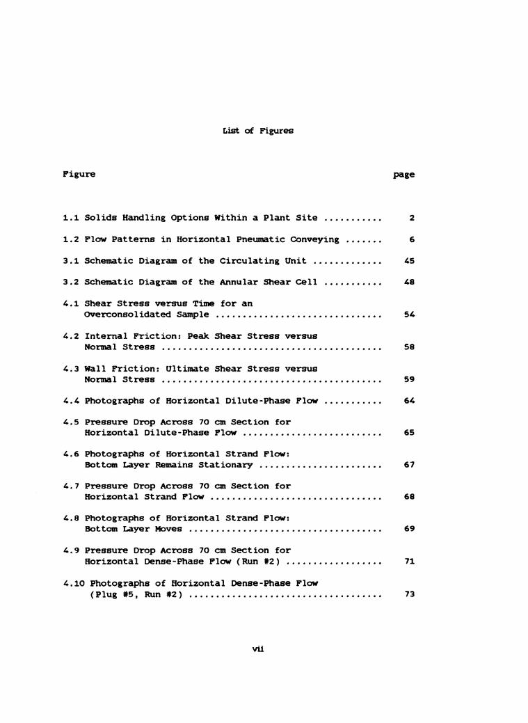


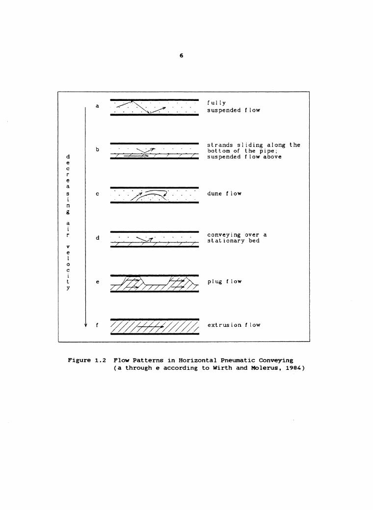


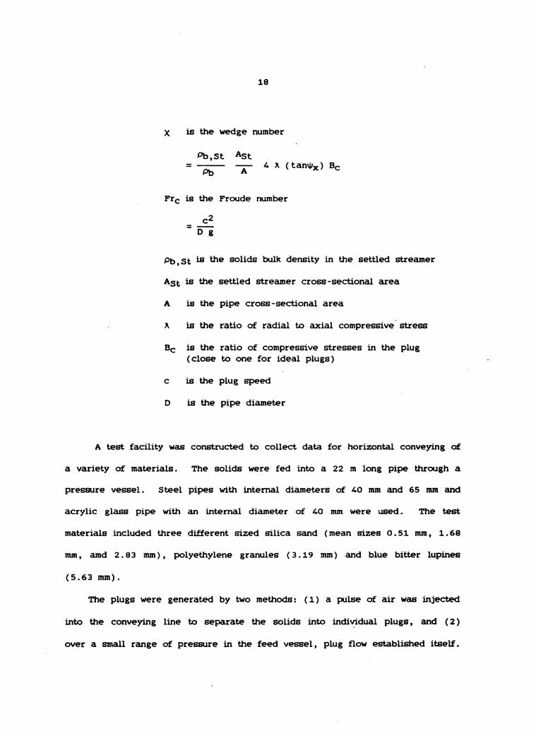


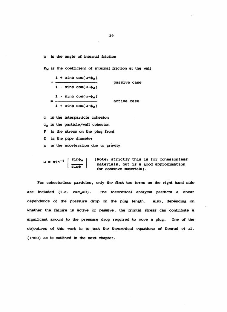

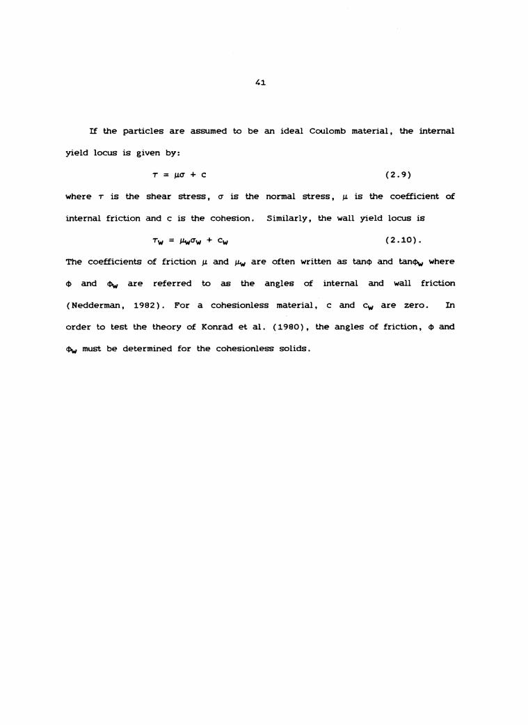
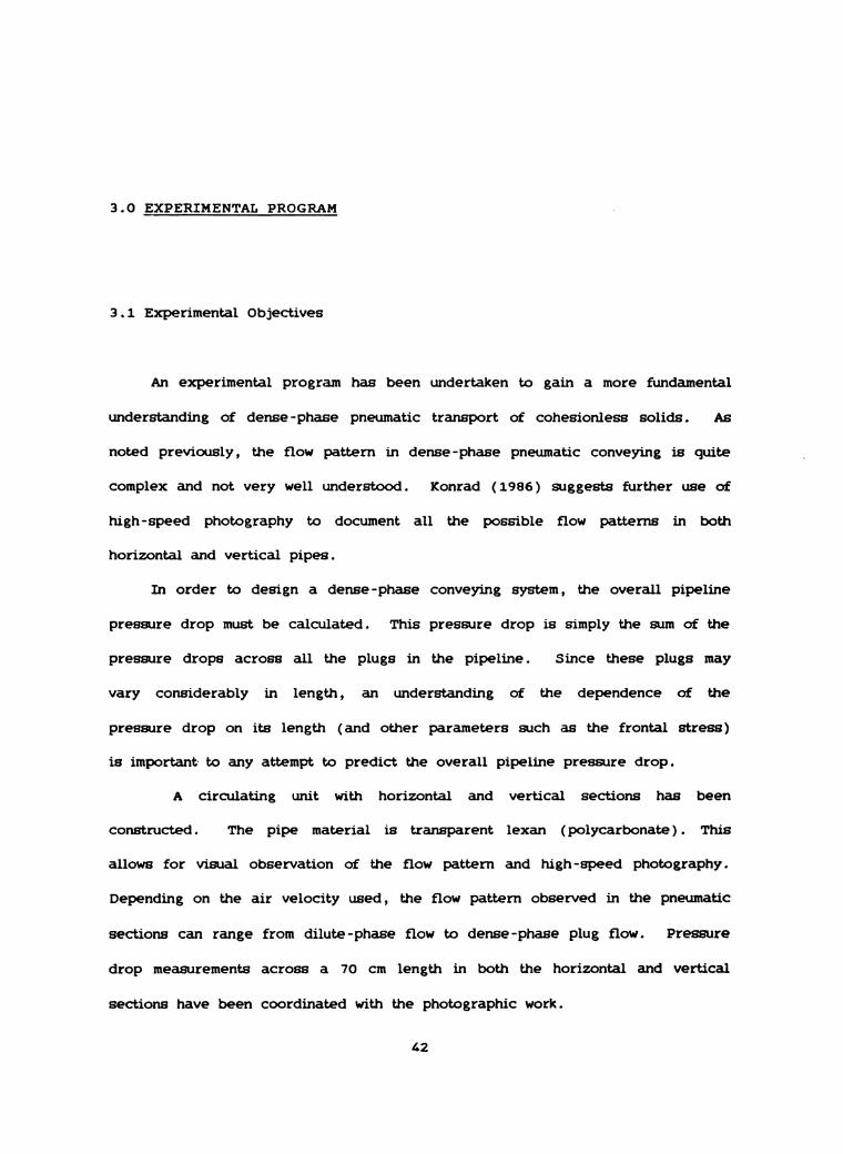
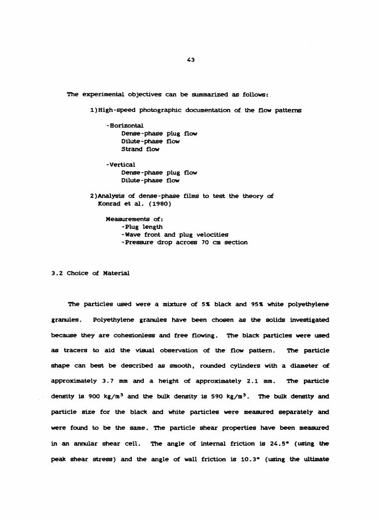

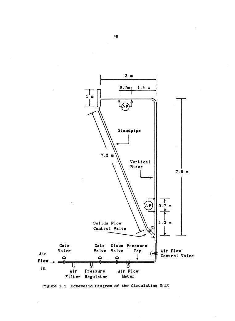


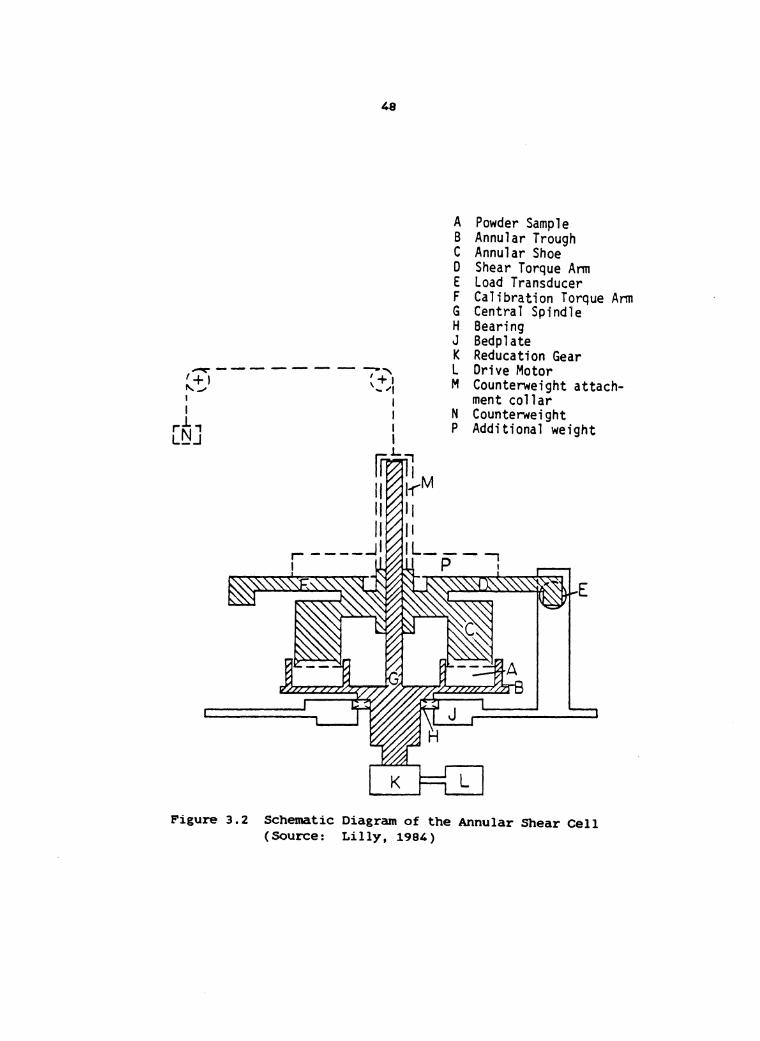


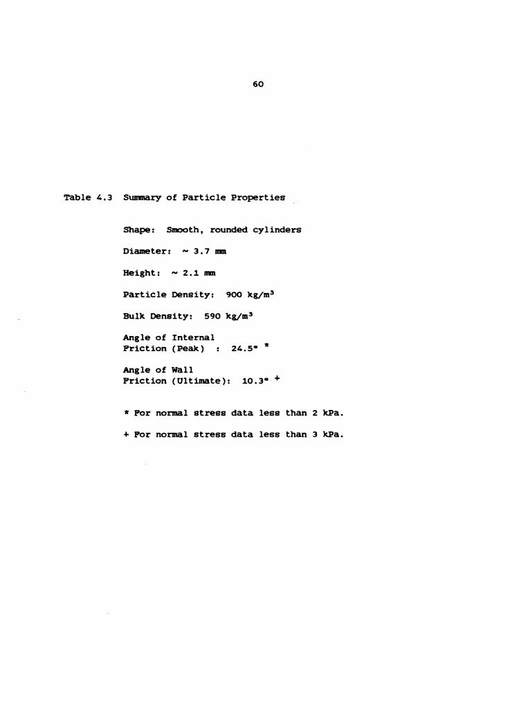


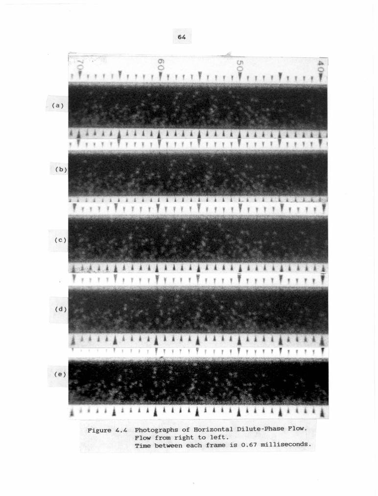
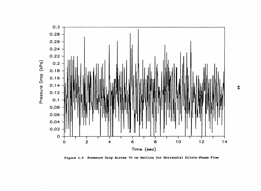


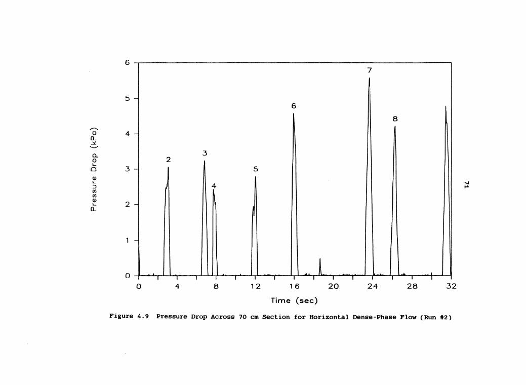


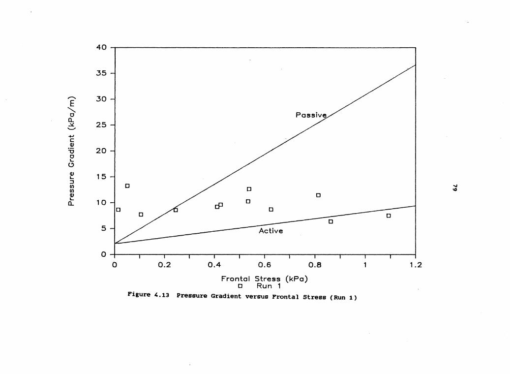


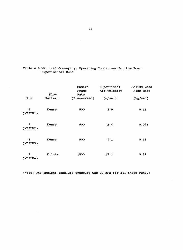


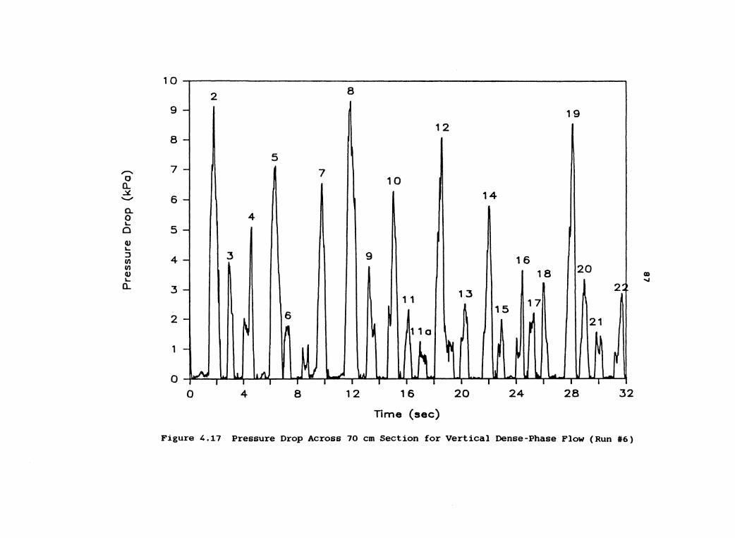
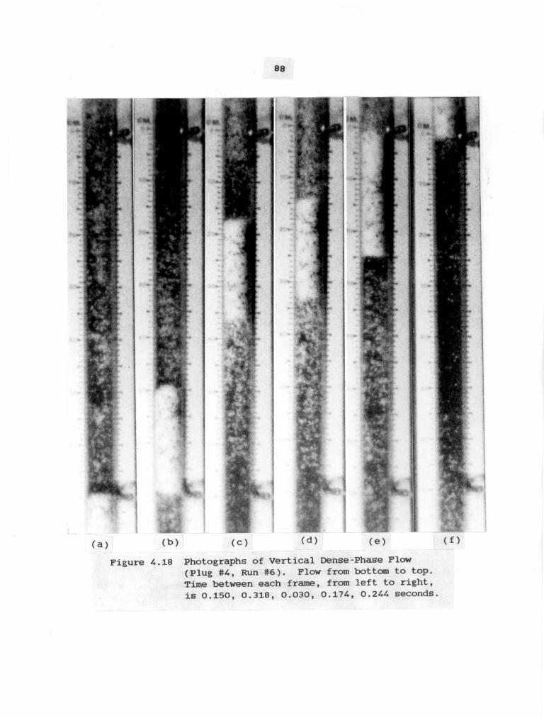


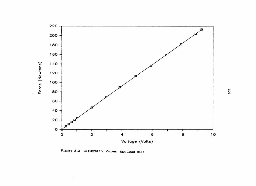


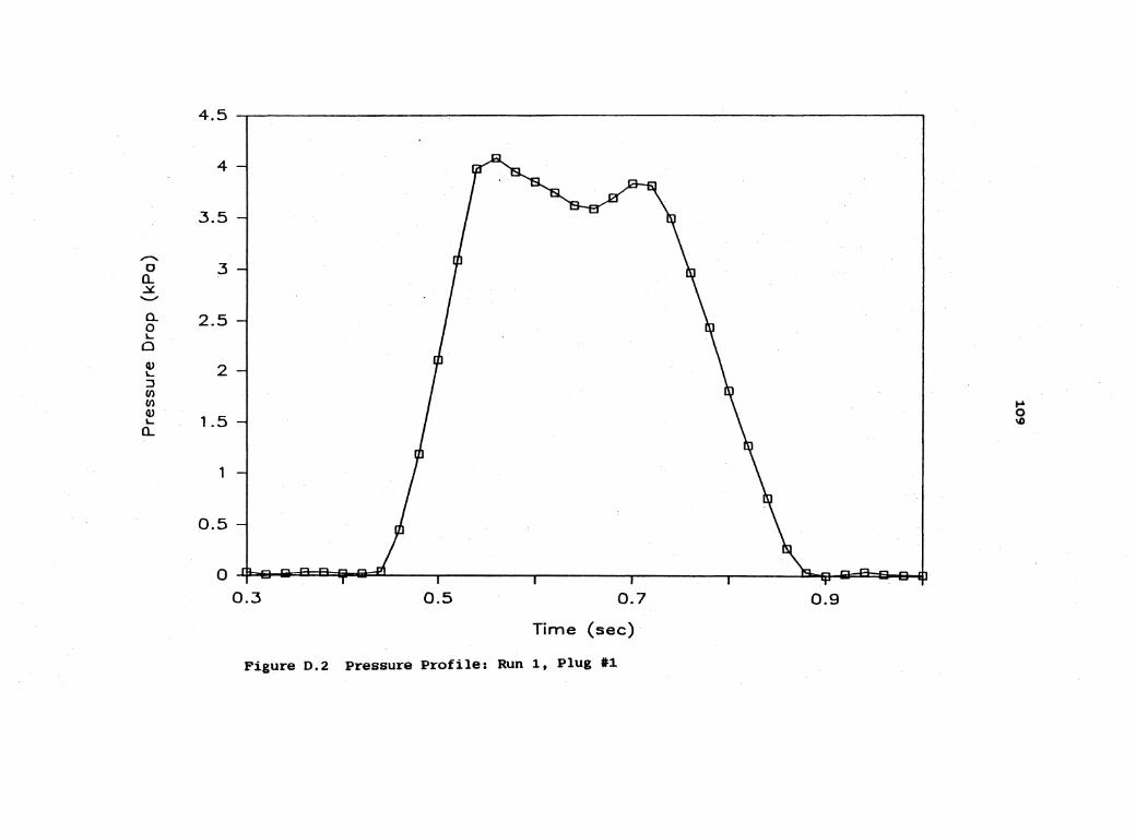
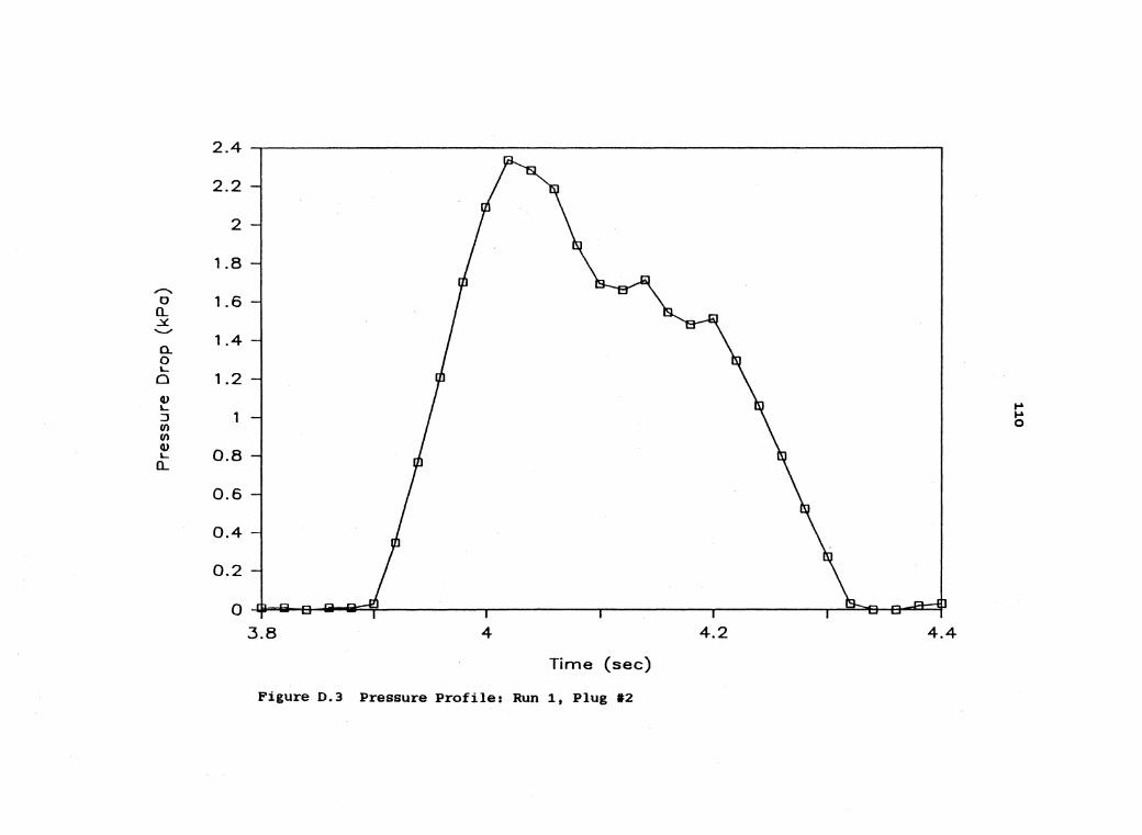

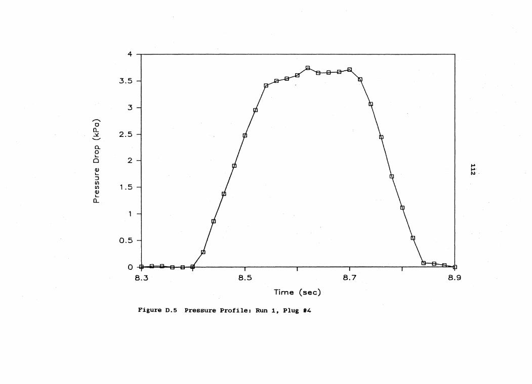
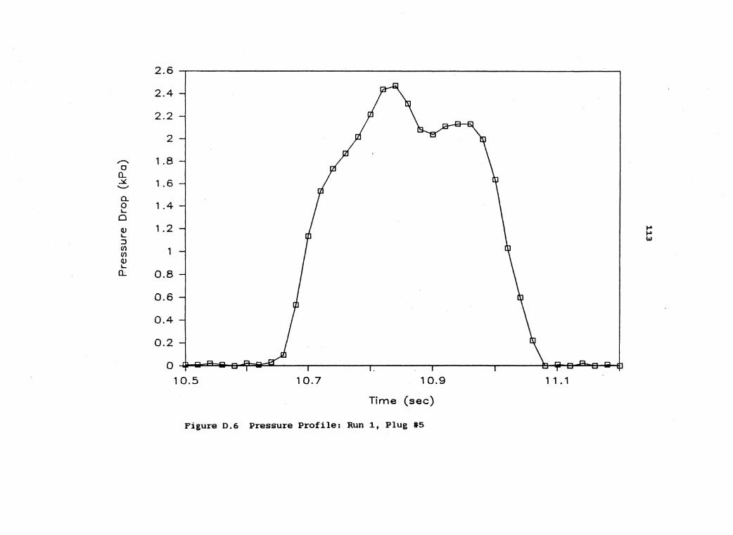

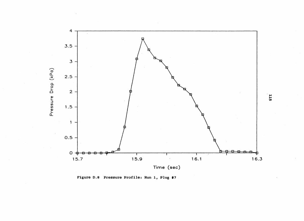

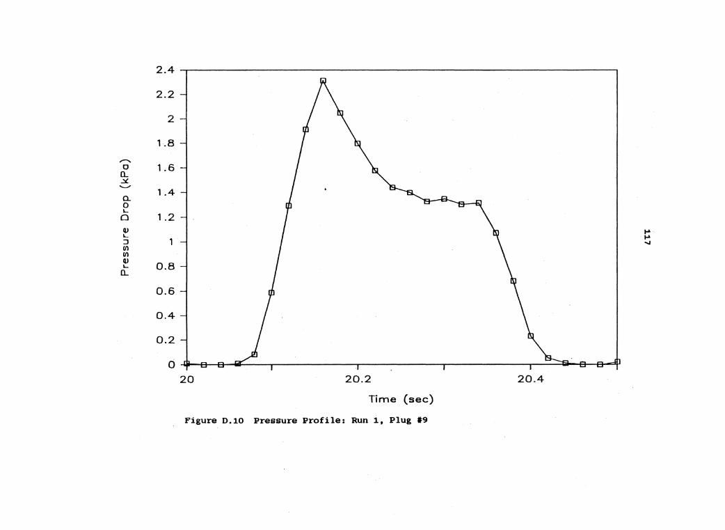
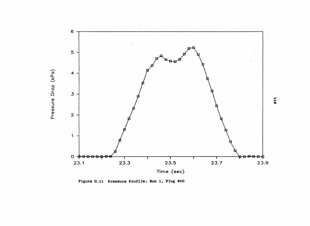

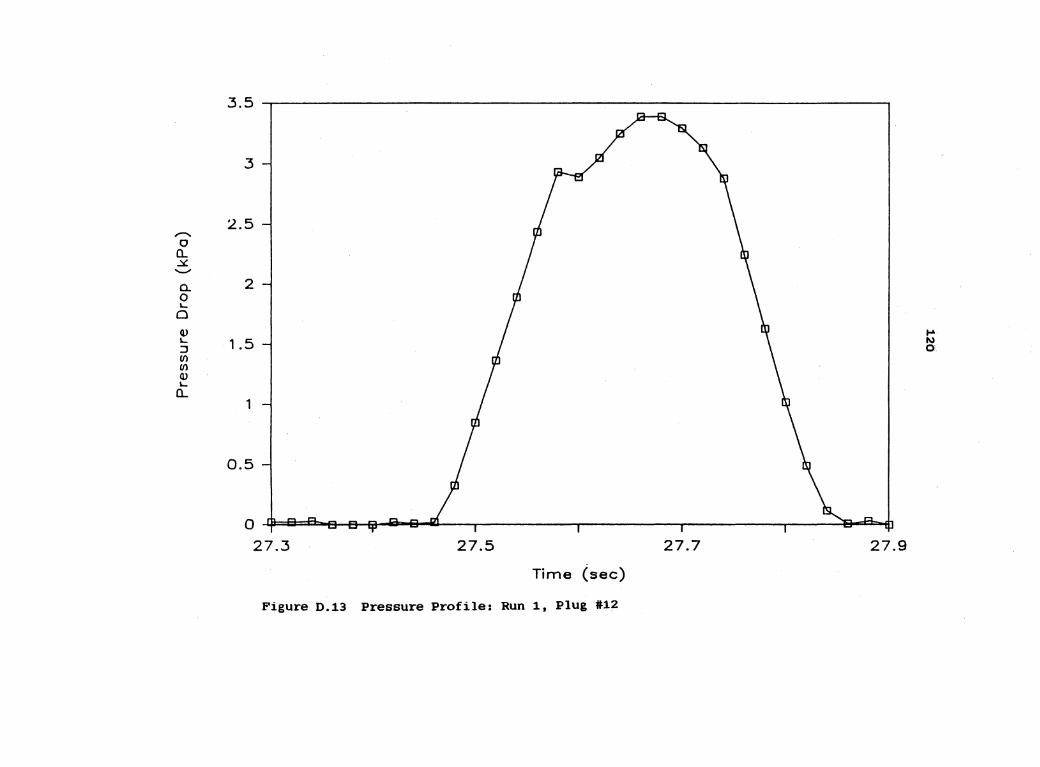


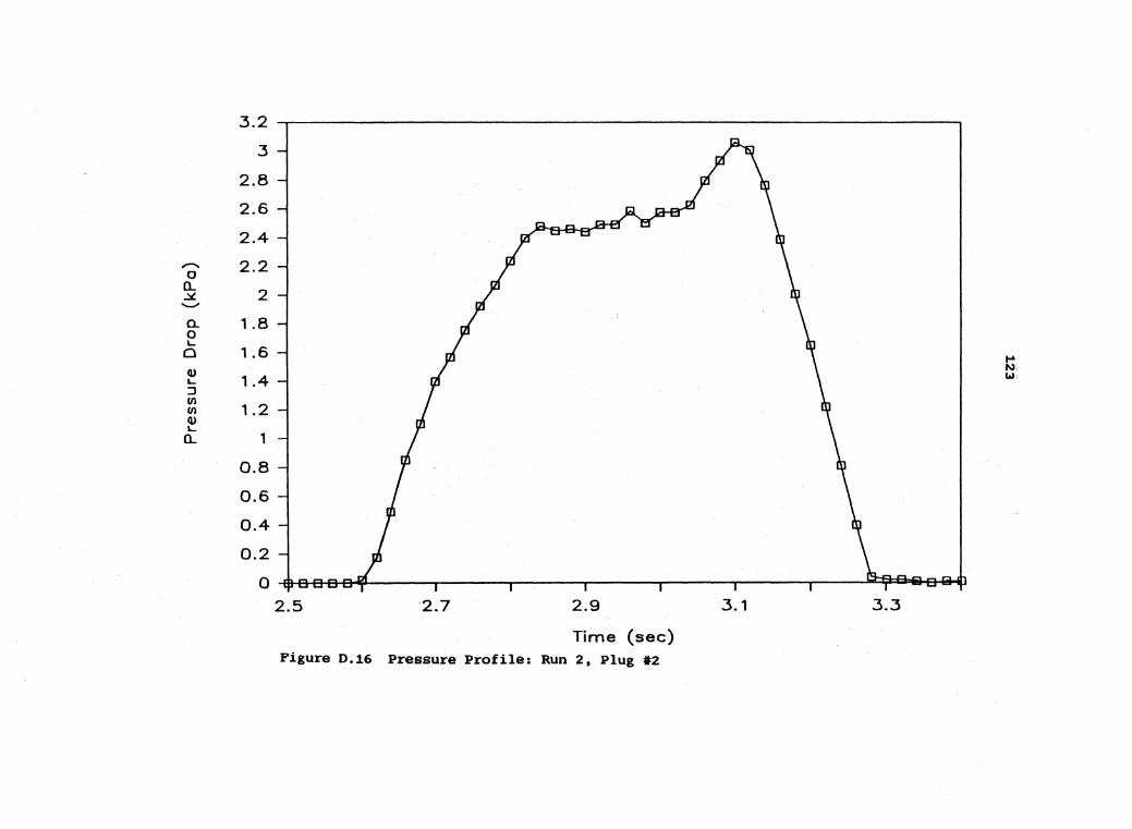

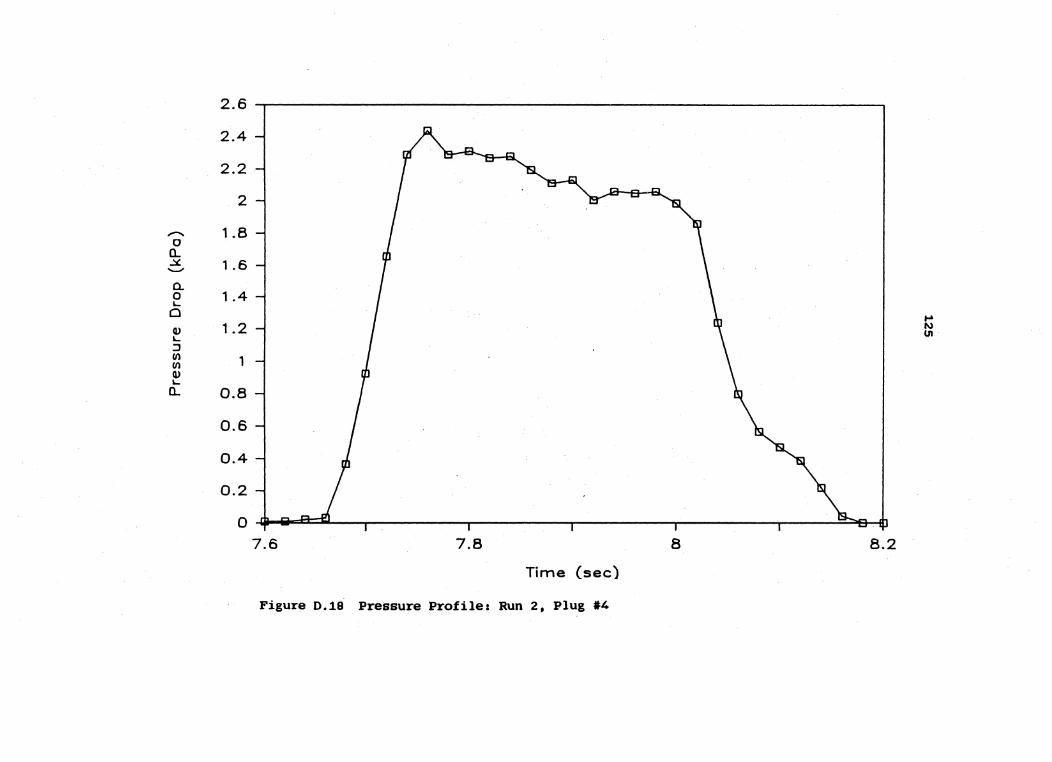


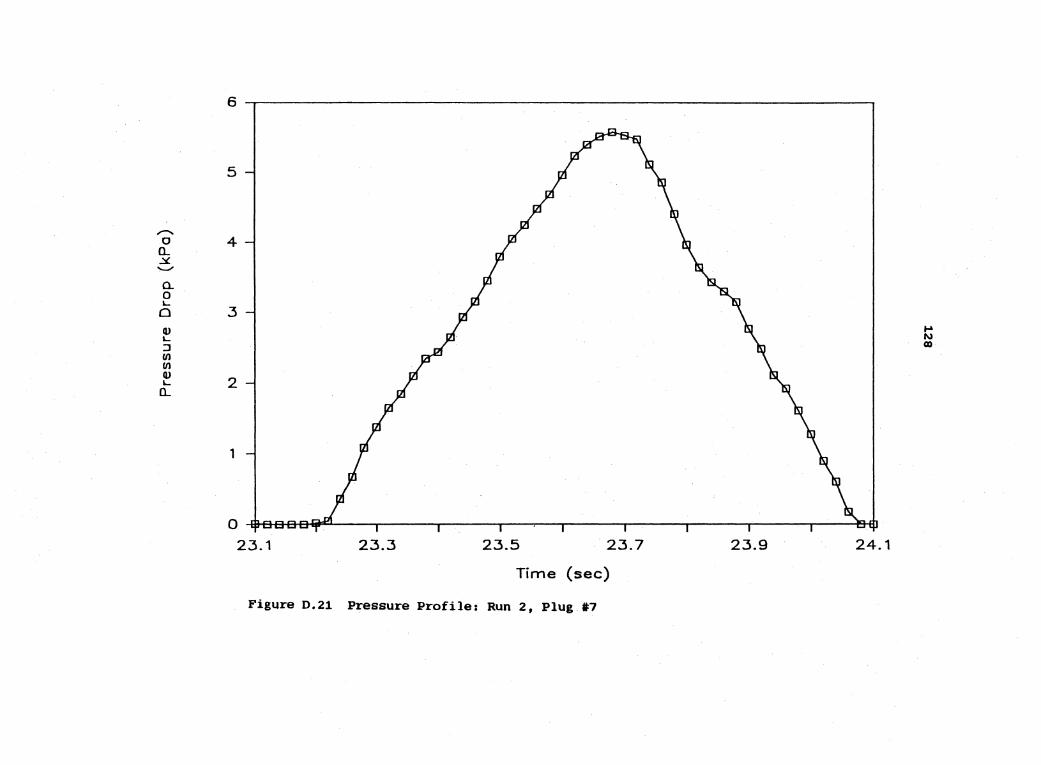
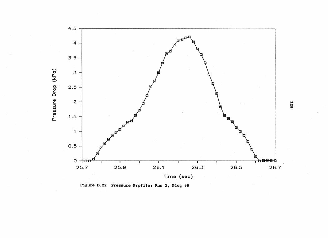
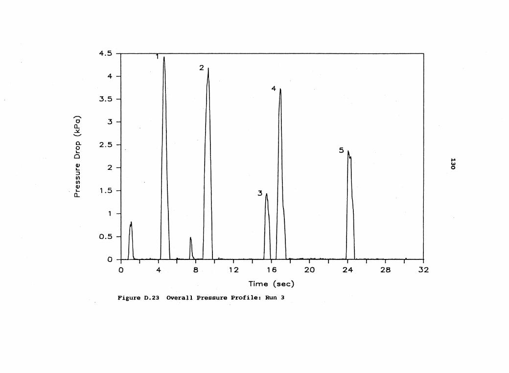


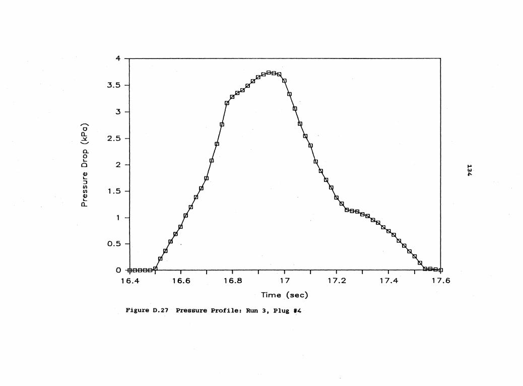


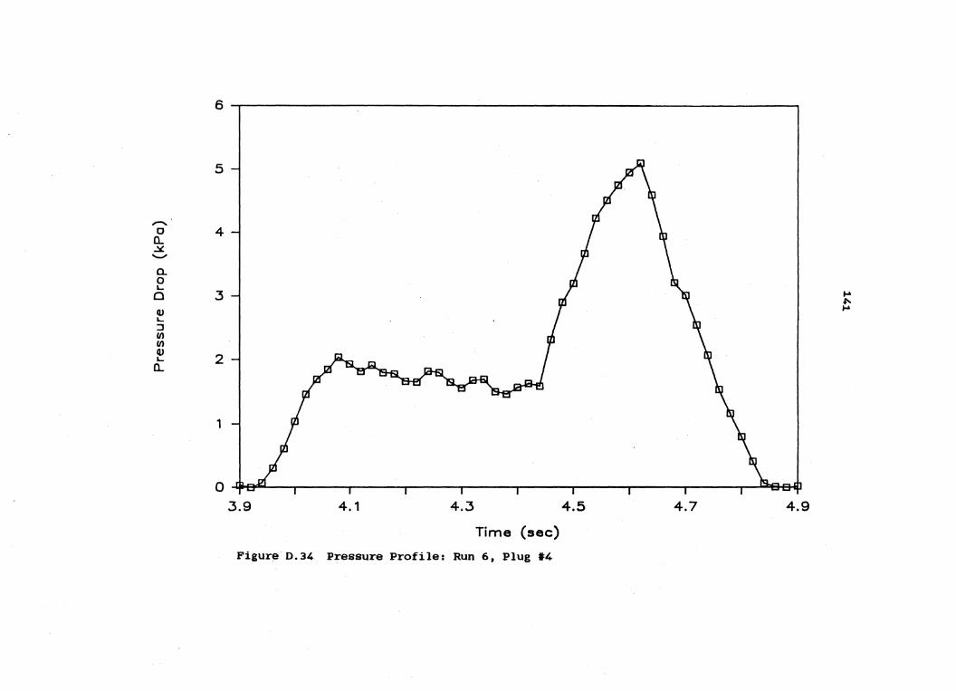


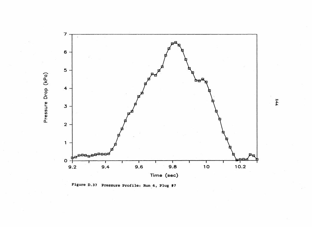


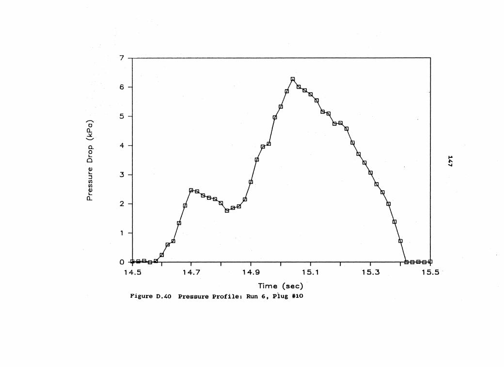
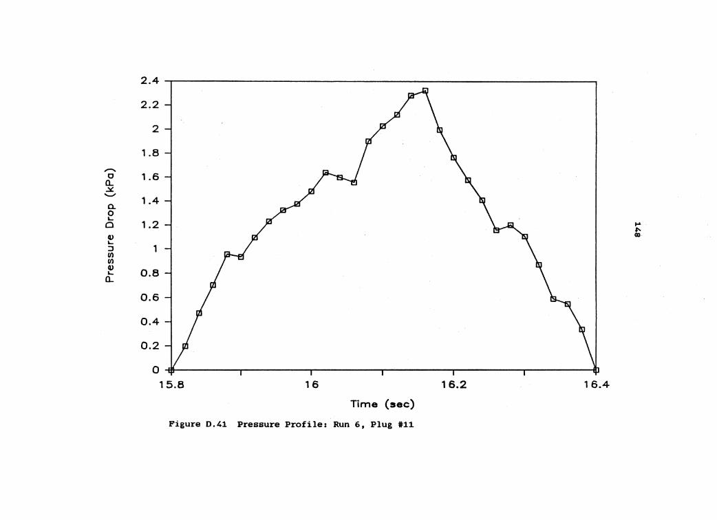


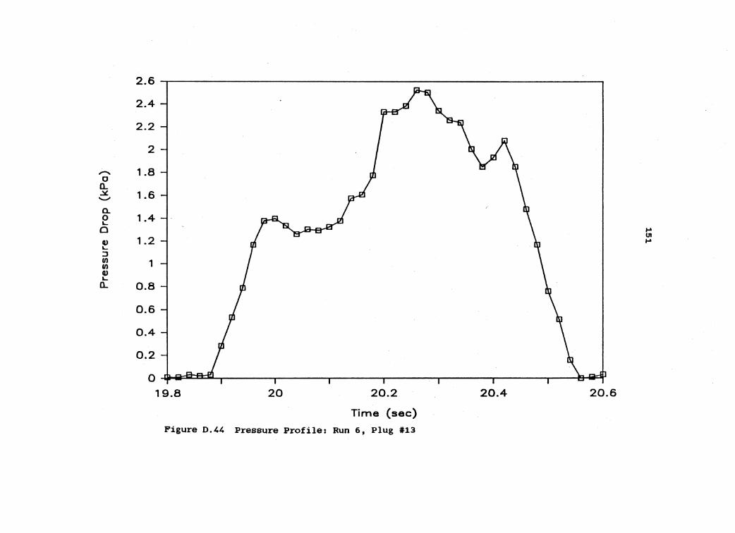
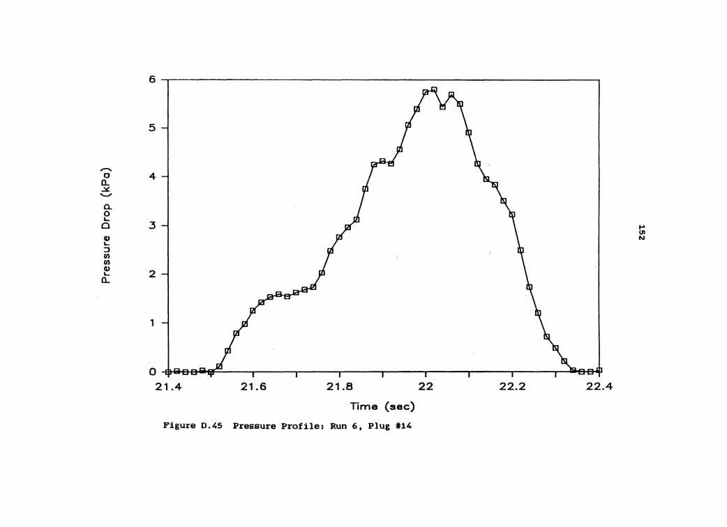


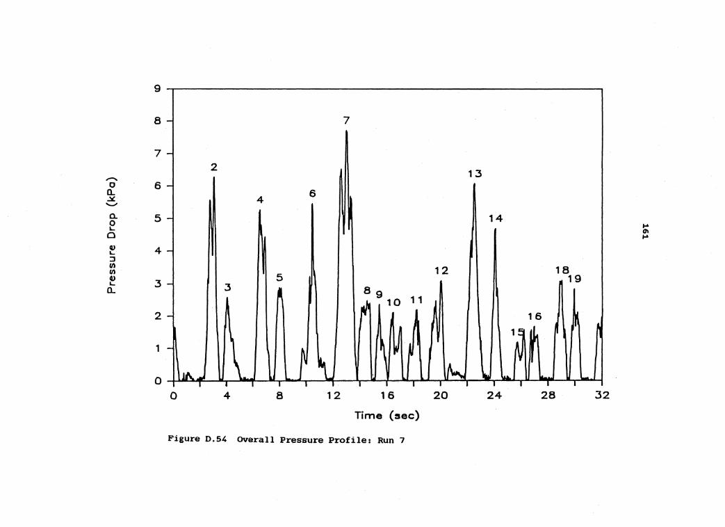
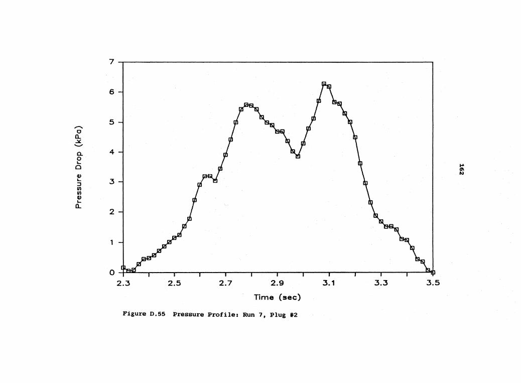

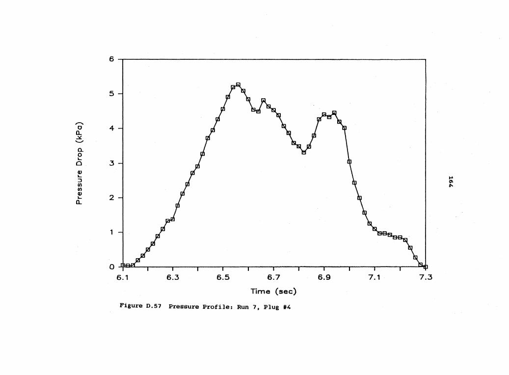


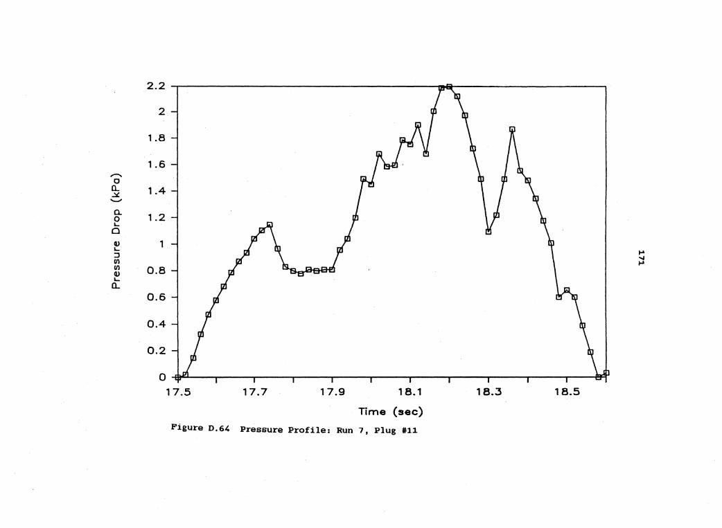

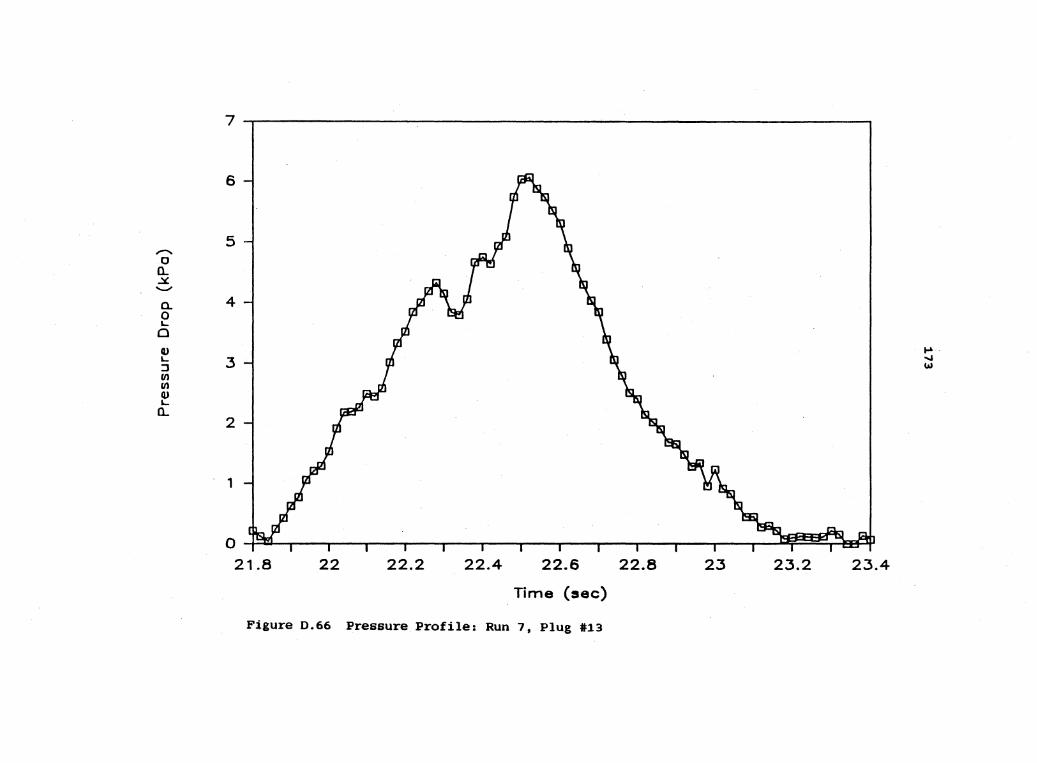

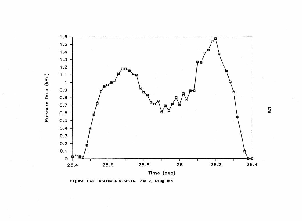


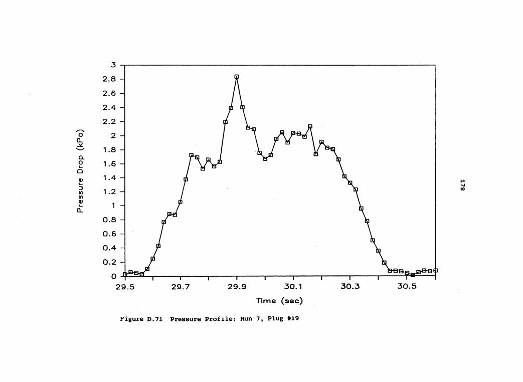
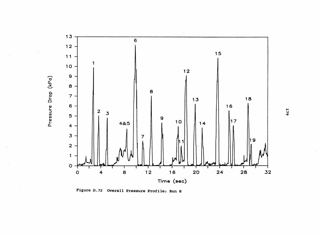

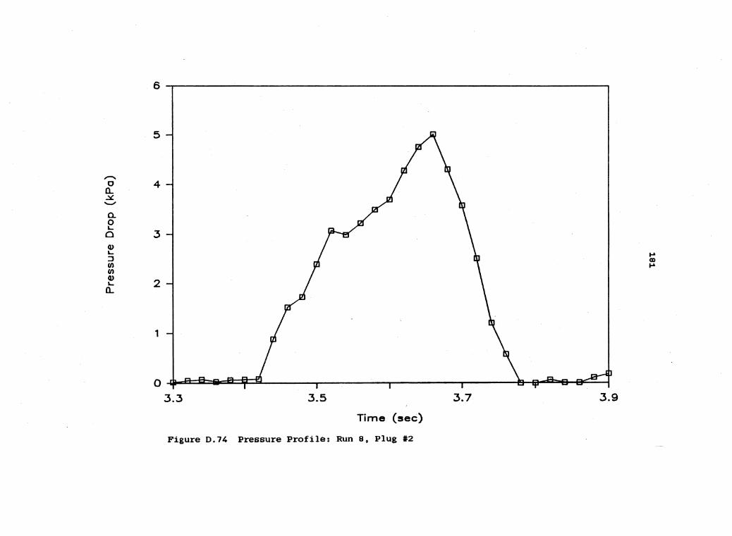
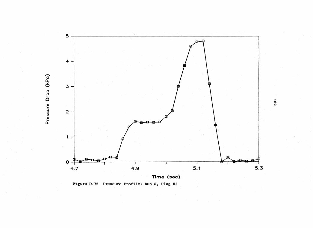


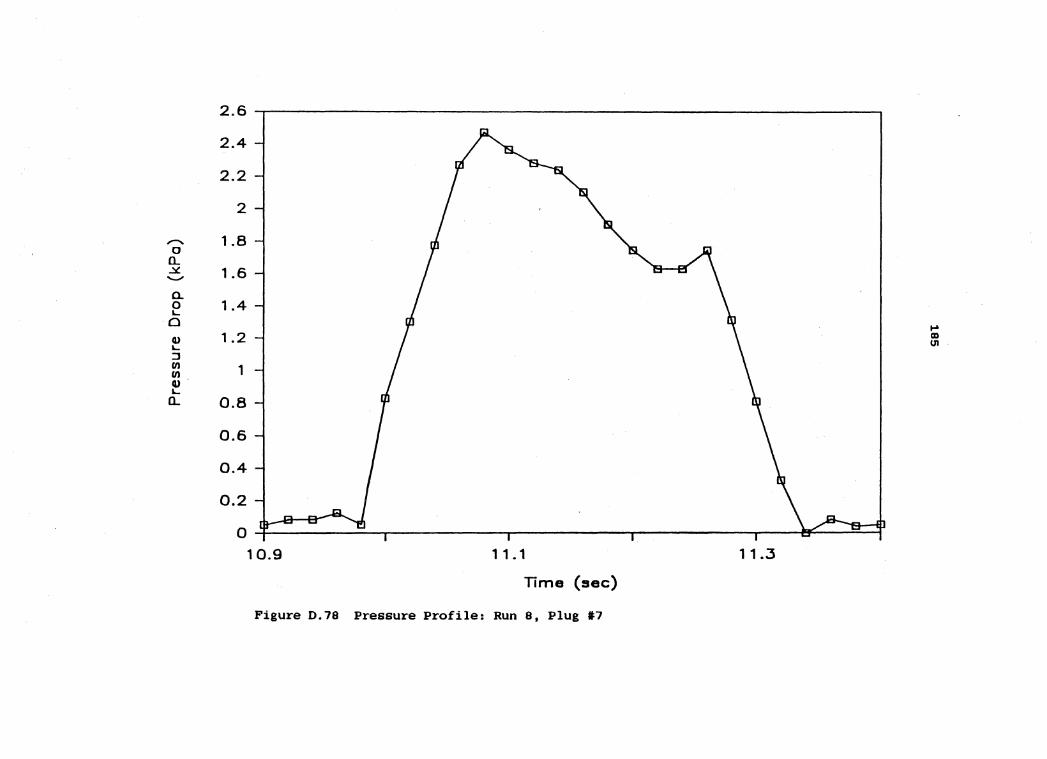


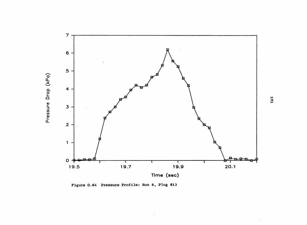


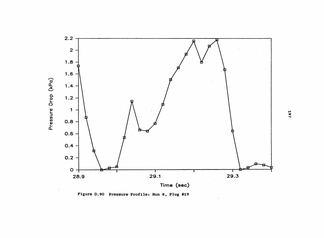


![3. Phase analysis · Web viewAs-well as inhibiting thermoelectric properties, porous solids are less mechanically robust than fully dense ones [20], which, combined with shape changes](https://static.documents.pub/doc/80x56/5fedb77a127a7e6bee7edcdd/3-phase-analysis-web-view-as-well-as-inhibiting-thermoelectric-properties-porous.jpg)