RADseq Data Analysis with Stacks in Galaxy DATE: 2017-02-01 VERSION: v0.1.2 UPDATED BY: Pip Griffin, Sonika Tyagi & Vicky Schneider Description This tutorial aims to introduce RADseq data processing from raw reads to SNP calls. The tutorial also introduces Galaxy, which is the analysis platform we will be using combined to the Stacks tools, a software pipeline for building loci from short-read sequences, such as those generated on the Illumina platform (http://catchenlab.life.illinois.edu/stacks/). We will cover a reference- genome-free approach and demonstrate the effect of some parameterization choices available. The tutorial also covers some initial approaches for downstream data exploration and analysis. It is accompanied by an introductory lecture that covers the aims, uses and limitations of the RADseq technique, and details of the molecular approach (es) to build RADseq libraries. Keywords LEVEL Beginner TOPIC DNA & RNA DURATION 2 hours
Transcript
RADseq Data Analysis with Stacks in GalaxyDATE: 2017-02-01VERSION: v0.1.2UPDATED BY: Pip Griffin, Sonika Tyagi & Vicky Schneider
Description
This tutorial aims to introduce RADseq data processing from raw reads to SNP calls. The tutorial also introduces Galaxy, which is the analysis platform we will be using combined to the Stacks tools, a software pipeline for building loci from short-read sequences, such as those generated on the Illumina platform (http://catchenlab.life.illinois.edu/stacks/). We will cover a reference-genome-free approach and demonstrate the effect of some parameterization choices available. The tutorial also covers some initial approaches for downstream data exploration and analysis. It is accompanied by an introductory lecture that covers the aims, uses and limitations of the RADseq technique, and details of the molecular approach (es) to build RADseq libraries.
Keywords
LEVEL Beginner
TOPIC DNA & RNA
DURATION 2 hours
After completing this tutorial you will be able to:
- Navigate the History and Tools panes in Galaxy, and view datasets in the viewing pane.- Read the FASTQ, bam/sam and vcf file formats.- Explore raw RADseq reads to identify the restriction enzyme overhangs.- Assess the importance of quality checking and parameters to look out for.- Run basic Stacks workflows in the Galaxy environment.- Extract sample-based and catalogue based summary statistics.- Explore VCF files
RADseq is a Restricted Representation Library technique for obtaining DNA sequence information from a replicable subset (usually ~1-5%) of a genome. This technique involves extracting total DNA and digesting it with one or more restriction enzymes. The resulting fragments can then be ‘barcoded’ by ligating a short, unique DNA tag, often joined to the adaptors needed for subsequent sequencing. ‘Selection’ of a replicable subset of fragments can be carried out by size-selection, PCR, or a variety of other approaches, depending on the exact protocol used. Multiple individuals can be pooled together and sequenced using next-generation technology (typically Illumina HiSeq or MiSeq).
RADseq is useful for population genetics, phylogenetics and plant/animal breeding studies where it is not necessary or practical to perform whole-genome sequencing. It typically generates thousands to hundreds of thousands of single nucleotide polymorphism (SNP) markers that can be used to infer population diversity and structure, individual relatedness, linkage maps, and/or evolutionary history.
Page 2
There are numerous variations on the original RADseq protocol, as described in Nature Reviews Genetics 17, 81–92 (2016) doi:10.1038/nrg.2015.28
• Single enzyme, indirect size selection. Genotyping by sequencing (GBS) uses a common-cutter enzyme, and PCR preferentially amplifies short fragments. Sequence-based genotyping (SBG)69 uses a rare cutter and one or two common cutters, and PCR preferentially amplifies short fragments.
• Double enzyme, indirect size selection. Complexity reduction of polymorphic sequences (CRoPS)70 uses two enzymes and a proprietary library preparation kit (originally developed for 454 pyrosequencing).
• Single enzyme, direct size selection. Reduced representation libraries (RRLs), are unique in using a blunt-end common-cutter enzyme, followed by a size selection step and a proprietary Illumina library preparation kit. Multiplexed shotgun genotyping (MSG) uses one common-cutter enzyme and a size selection step. ezRAD uses one or more common-cutter enzymes, and a proprietary kit for Illumina library preparation.
• Double enzyme, direct size selection. Double-digest RAD (ddRAD) uses two restriction enzymes, with adaptors specific to each enzyme, and size selection by automated gel cut.
Variations on the above techniques include using methylation-sensitive enzymes; adding more restriction enzymes to existing protocols to further reduce the set of loci; adding a second digestion to eliminate adaptor dimers; adapting RADseq techniques to other sequencing platforms such as Ion Torrent; and other minor technical modifications.
Researchers should be aware of the limitations and biases of their chosen method and tailor their downstream analysis accordingly.
What is Stacks?
Stacks is a set of software tools for processing RADseq data developed by Julien Catchen at the University of Illinois (http://catchenlab.life.illinois.edu/). It has a fairly large user base, and is in ongoing development. Stacks issues can be raised in the Stacks google group (https://groups.google.com/forum/#!forum/stacks-users).
Stacks can be used to:
generate mappable markers from RAD-seq data. identify SNPs within or among population perform phylogenetic analysis of GBS/RADseq data.
What is Galaxy?
Galaxy is a free, open-source software that acts as a user-friendly interface to tools for data processing and analysis. Users can run common bioinformatics software like Trimmomatic and bwa within Galaxy, and build their own workflows. Users can also share workflows and data processing histories. The Stacks tools have been wrapped for Galaxy and can be installed from the Galaxy Toolshed. The Galaxy Toolshed is the software repository for Galaxy.
What is the GVL?
The Genomics Virtual Laboratory is a data processing and analysis platform. It provides a cloud-based suite of genomics analysis tools (including a way to get Galaxy) that would normally require specialist assistance. The Genomics Virtual Lab (GVL) project uses computing resources from the NeCTAR Research Cloud. For more information about the GVL, see here https://www.gvl.org.au/
Relevant Concepts Restriction enzyme digestion
The process that uses restriction enzymes (enzymes isolated from bacteria that recognize specific sequences in DNA) to cut the DNA, producing fragments called restriction fragments.
Barcoding and multiplexingA barcode is a short, unique nucleotide sequence identifying reads that come from a specific individual. The most common barcoding design uses inline barcodes occurring at the start of Read 1, located after the sequencing adaptor. Read 2 in paired-end sequencing only has an inline barcode if you have used a combinatorial barcoding approach.
Multiple samples can be run as single Illumina library by using a unique in-line barcode for each sample. The process is called multiplexing. The unique barcodes can then be used to assign reads to the individual samples they came from, using a bioinformatic process called demultiplexing.
Combinatorial barcoding: Using a pair of barcodes: usually with one barcode located on each end of the sequenced fragment. Different length barcodes can also be used to increase the number of possible combinations.
Illumina sequencing:A next-generation, high-throughput sequencing-by-synthesis approach that recognises bases by their fluorescent labels as they are added to a synthesised sequence. Illumina is a company that develops sequencing technologies. Its most commonly used sequencer machines are the HiSeq (very high throughput, rather slow); MiSeq (lower throughput, fast) and the newer NextSeq (intermediate throughput and rather fast).
Paired-end sequencing A kind of next-generation sequencing approach that involves sequencing both the start and the end of a DNA template fragment. For example, a common Illumina HiSeq library design would be to sequence 100 bp from the start, and 100 bp from the end, of fragments that are ~400 bp in length. https://www.illumina.com/technology/next-generation-sequencing/paired-end-sequencing_assay.html
Single nucleotide polymorphism (SNP)SNP (pronounced ‘snips’) represent a single nucleotide difference in the DNA. In most taxa, SNPs are the most common type of genetic variant among and within individuals.
Genetic diversityVariation in genetic makeup within and among species.
Population divergenceThe level of genetic differentiation between two or more populations of an ancestral species, which can accumulate independent genetic changes (mutations) through time.
Vocabulary associated with the Stacks program Stacksa software pipeline developed by Julian Catchen et al. to process restriction enzyme based next-generation sequencing data such as RAD-seq data. stack a ‘pile’ of aligned sequence reads from one individual judged to come from the same genomic location.
Page 4
RADtag, RAD marker, tagsequence that flanks a restriction enzyme recognition site. “Restriction site associated DNA (RAD) tags are a genome-wide representation of every site of a particular restriction enzyme by short DNA tags.” (Miller et al. 2007) – but whether your RADtags really come from every site of a particular restriction enzyme will depend on the molecular approach you used. primary reads reads that are used for the first iteration of stack building in ustacks. secondary readsadditional reads added to the stack in the second iteration of stack building in ustacks. batcha set of samples processed in the same data processing run
cataloguea set of tags, and the corresponding haplotypes and genotypes, for a batch of samples. The catalogue can be generated from all samples in a batch or from a subset of samples (usually parent samples in a genetic mapping experiment).
Where does the tutorial data come from?
This dataset comes from a real experiment performed by researchers in the Hoffmann Lab, School of BioSciences, University of Melbourne. This experiment aimed to investigate the genetic population structure among Aedes aegypti populations in Australia/South-East Asia. Aedes aegypti is a widespread tropical mosquito species that can transmit the dengue, yellow fever, chikungunya and Zika viruses. Understanding its population structure is crucial for managing efforts to prevent mosquitos from transmitting viruses by infecting them with Wolbachia bacteria, an infection that can spread naturally through mosquito populations given the right evolutionary conditions.
Here we are using data from 2 individual mosquitos from just 2 populations, Kuala Lumpur (HKL) and Bangkok (BKK). The reason for using a sub-sample of the original dataset is merely to allow Stacks jobs to finish within the limited time we have today. The data has been down-sampled to include only 50% of the original sequence reads per sample.
Who is this tutorial for?
Students and researchers using or critically engaging with raw RADseq data or SNPs generated with RADseq, as beginners
Students and researchers who want an overview of the data processing involved in a typical RADseq experiment
Students and researchers new to bioinformatics who are less comfortable with command-line tools
Students and researchers who want an overview of the kinds of functionality available in Galaxy for RADseq data processing and downstream analysis
Page 5
ATTENTION BOX To access Stacks in Galaxy for use on your own data once you have completed this tutorial, there are two main options:
When to use Stacks in Galaxy
when you are learning the steps and data formats involved in RADseq data processing when you are not so comfortable with command-line programming when you don’t need the Stacks web interface when somebody has shared a Stacks Galaxy workflow or history with you
When not to use Stacks in Galaxy
when you prefer to use command-line Stacks over the GUI-based Stacks in Galaxy when your Galaxy instance has insufficient memory or compute for your data when you are running jobs on high-performance computing resources via the command line when you want to use a Stacks version that is not wrapped for Galaxy
How to access and navigate Galaxy for this tutorialThis assignment will use the program Galaxy, through a cloud-based computing platform called the Genomics Virtual Lab.
Page 6
STEPS BOX 1. To access the Galaxy instance for this assignment, open a web browser and type in
the address bar
http://game-2.genome.edu.au/galaxy
2. Register as a Galaxy user. Have a look at the tabs across the top of the screen. You should see these options:
Click on ‘User’ → ‘Register’. Enter your email address, a password you can remember and a short username. Click ‘Submit’
ATTENTION BOX To access Stacks in Galaxy for use on your own data once you have completed this tutorial, there are two main options:
HELP BOXThe Galaxy interface contains three windows: your History (on the right-hand side of the screen); a list of the available data analysis Tools (on the left-hand side); and the central display area, where you can specify analysis tool settings and visualize data
STEPS BOX 3. Get the data for this assignment.
Look at the tabs across the top of the screen again and click on the one called ‘Shared Data’ → ‘Published Histories’
This should take you to a page where you can see a history called fastq_files. Click on the name, then click on the option ‘Import History’ near the top right-hand corner of the screen.
This will make a copy of the data files for you to work on. Give the new history a name of your choosing and click ‘Import’.
Your History window should now display 9 data files that you imported from the fastq_files shared history.
HELP BOX The same login details will let
you log in to your personal Galaxy portal again, so you
can come back to your work if you need to log out part-way
through. It will save automatically.
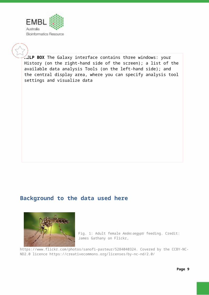
Background to the data used here
Fig. 1: Adult female Aedes aegypti feeding. Credit: James Gathany on Flickr, https://www.flickr.com/photos/sanofi-pasteur/5284040324. Covered by the CCBY-NC-ND2.0 licence https://creativecommons.org/licenses/by-nc-nd/2.0/
Fig. 2: World map showing the predicted distribution of Aedes aegypti (red: 100% occurrence probability; blue: 0% occurrence probability). From Kraemer et al. (2013) eLife http://dx.doi.org/10.7554/eLife.08347.004
Aedes aegypti is a widespread, human-associated disease vector. It spreads dengue, chikungunya, Zika and yellow fever viruses (among other things) and occurs in most tropical regions of the globe. It is well adapted to living with humans, active in
the daytime and can lay eggs in very small volumes of water like potplant saucers, buckets and old tyres.
Currently there is no vaccine for the dengue virus (which infects almost 400 million people per year, 0.5 million of whom require hospitalisation) and the main means of control is insecticide spraying. However, Aedes aegypti readily evolves resistance to insecticides. More recent control measures have involved attempts to cause population extinction (by releasing large numbers of sterile males) and attempts to infect Aedes aegypti populations with Wolbachia bacteria, which appears to block virus transmission.
Wolbachia naturally infects many insects (though not Ae. aegypti) and causes a phenomenon called cytoplasmic incompatibility, which gives infected females a selective advantage, causing the infection to spread through the population. This spread of Wolbachia infection however will only occur under certain evolutionary parameters (e.g. sufficient starting frequency, sufficient dispersal rates, well-mixing populations etc.) Therefore, to manage a Wolbachia release into a natural mosquito population, a large amount of background information is required about the size, structure and diversity of that particular population.
Aedes aegypti has a fairly large genome (~1.4 Gb) that consists of approx. 70% repetitive regions. Microsatellite genotyping provides only coarse population genetic information for this species, while whole-genome sequencing would be costly and ‘overkill’ in terms of the resulting marker numbers. By using RADseq, researchers can obtain thousands of single nucleotide polymorphism markers for an affordable per-sample cost.
RADseq requires both molecular expertise (to design and prepare libraries) and bioinformatic expertise (to process and analyse the resulting data). Each of these can be outsourced, but it is important for people at either end of the process to understand the context, research aims and limitations.
This experiment used Double Digest RADseq (ddRADseq) as outlined in Rasic et al. (2014). The samples were barcoded using combinatorial barcodes: one on Read1 and one on Read2.
Page 9
Fig. 3: A typical workflow for processing RADseq/GBS data. Taken from https://github.com/thierrygosselin/stackr, Credit: Thierry Gosselin
Page 10
Exercises
These exercises provide examples of how Stacks in Galaxy can be used and test your knowledge by asking you questions about the tasks and results. Exercise 1: Raw RADseq reads – exploration and quality checking
1.1Have a look at one of the raw FASTQ files (e.g. BKK30_downsampled_1.fq).
1.2 Click on the file name in your Galaxy history (on the right of the screen) to expand the history entry to show some basic information about this file. 1.3 Click on the eye icon: this will show the start of the file displayed in the display area in the centre of your screen.
Page 11
ATTENTION BOX Avoid clicking ‘Show All’! The file is about 700 MB in size and Galaxy may struggle to print the whole file to the screen.
SPECIAL NOTE BOX FASTQ files contain DNA sequences and quality information for each sequencing read, in FASTQ format. This text format consists of four lines per read: an identifier line (starting with ‘@’), a sequence line, a third line that can include the same identifier (starting with ‘+’), and a quality score line.
For example
@SN7001291:346:HFMF3BCXX:2:1101:1148:1934
AACCCCGTGGGAACCAAGGTGCAGTTANGGATGATT…
+
!’’*??AQRWXXYZ^^ZjklYPOLWKZ?ADFLMMOP…
Paired-end sequencing produces two reads per DNA fragment: one from the start of the fragment (called Read 1) and one from the end of the fragment (called Read 2). These are typically presented in two separate FASTQ files and can be matched by the identifier line.
1.4 Calculate some summary and quality assessment statistics.
In the tool list on the left-hand side, select ‘NGS Analysis → ‘NGS: QC and manipulation → ‘FastQC’.
The default option is to apply this tool to one dataset in your History, which you can choose using the drop-down menu. Instead, try applying this tool to all the files. Click the ‘multiple datasets’ symbol and hold down the Shift key to select all 8 FASTQ files.
Leave the other options with their default values and click ‘Execute’.
You will see some new jobs appear at the top of your history panel; they will be coloured grey while they’re waiting to run, yellow while they’re running and turn green
Page 12
HELP BOX If you are trying to execute a job in Galaxy and it’s not working, or if you want to repeat the execution with different settings (e.g. if you chose the wrong input file originally), click on the name of the job in your History to expand the view, and click the arrow icon under the file name (hover-over says ‘Run this job again’). This will allow you to adjust the execution settings and rerun the job.
HELP BOX If you are having difficulty understanding how to use Galaxy – or if you just want to know more about what you can do with Galaxy – you can consult this introductory tutorial http://vlsci.github.io/lscc_docs/tutorials/galaxy_101/galaxy_101/
when it’s finished successfully. If a job fails, it will be coloured red, and should give you an informative error message.
Q1: How many jobs are spawned for each input dataset? How can you tell which dataset a job has run on?
Once it’s ready, click on the name of one of the jobs described as a Webpage result to see some basic information. View it with the eye icon to display the html result file in the Display Area.
Q2: What do you think about the overall quality of this raw sequence data? Would you choose to do some quality trimming at this point in your workflow? If so, what parameters would be the most important to control?
We are going to skip trimming in this tutorial (though feel free to do it if you need an extra challenge) and move straight to aligning our raw reads into stacks, without a reference genome.
Page 13
Exercise 2: The Stacks workflow for reference-free alignment, catalogue-building and SNP calling
The Stacks workflow for reference-free alignment has three steps:
ustacks cstacks sstacks
Today we are going to run a single wrapper tool that executes all three steps in succession: denovo_map.pl
Q3: Can you locate the denovo_map.pl tool? Discuss with your neighbour to find a second way to locate this tool.
Click on denovo_map.pl and select the ‘Population’ usage option (our samples are from a population study, not a genetic map study).
Highlight only the Read 1 datasets to use in building stacks and specify the ‘popmap.txt’ dataset as the population map.
Then, expand the ‘Assembly Options’ tab by clicking on it. To choose your options here, visit http://tinyurl.com/stacks-settings and add your name in the ‘Name’ column. Set your Assembly Options in Galaxy as per the settings in the spreadsheet row you’ve chosen. This will allow us to assess how different denovo_map.pl settings affect the results. Leave the ‘SNP Options’ settings as the defaults.
Execute this job. It will take some time to run – at least 1 hour – so we will come back to this at the end of the session. For now, import some results that were prepared earlier. This history is called ‘denovo_map_output’. Save this as a new history.Examine the results of denovo_map.pl.
You will notice this job produced a lot of output files. There are results here for each individual at the tag, allele and SNP level that were generated by ustacks; catalogue match results that were generated by sstacks; and a useful log of steps run and results along the way.
Look at the output file that starts ‘denovo_map log with Stacks…’.
Q4: Can you identify the sections of this log that report on the running of ustacks, cstacks and sstacks?
Q5: Find the mean coverage depth per individual. Do you think these individuals were sequenced deeply enough? What would you gain by performing more sequencing?
Q6: How many loci does the final catalogue contain?
Q7: How many loci were kept after running sstacks?
Look at the dataset list that starts ‘Full output of denovo_map.pl…’ Here you can see the result files for the individual datasets: tags, alleles, and snps for each individual, and matches to the catalogue that was built from all 4 individuals. You will need to consult the Stacks manual to understand the format of each of these files: http://catchenlab.life.illinois.edu/stacks/manual/#files
Q8: Can you identify a stack that included some reads assembled as secondary reads? Why are these particular reads classified as ‘secondary’?
Q9: Looking at one of the individual ‘alleles’ files, can you identify a genotype that looks suspicious to you? Identify the same locus in the corresponding ‘tags’ file. Does this reveal any problems or issues? If so, what setting would you adjust to avoid this?
Q10: Look at one of the individual ‘matches’ files. What does this file contain? Which column tells you the catalogue locus ID? Which column tells you the individual locus ID?
Page 15
HINT BOX Look in one of the ‘tags’ files for the breakdown of reads into primary and secondary reads. Check the denovo_map settings in the spreadsheet (name: Pip) to understand how you were classifying primary (vs secondary) reads.
HINT BOX Consult the manual (http://catchenlab.life.illinois.edu/stacks/manual/#files) to see how the loci are identified in the individual ‘alleles’ and ‘tags’ files.
Select ‘Stacks 1.40’ ‘populations’. Specify the dataset that starts ‘Full output from denovo_map’ and specify ‘popmap.txt’ as the population map file.
To keep all loci that were called in any of the individuals we’re looking at, set the following parameters:
Set ‘Minimum percentage of individuals in a population required to process a locus for that population (-r)’ setting to 0
Set the ‘Minimum number of populations a locus must be present in to process a locus’ (-p) to 1
Restrict the analysis to one random SNP per locus set ‘Output results in Variant Call Format (VCF)’ to ‘Yes’ set ‘Enable SNP- and haplotype-based F-statistics’ to ‘Yes’ leave the other settings as defaults
Q11: Why might you choose to restrict the analysis to one random SNP per locus? What are the benefits and disadvantages of this choice?
Page 16
SPECIAL NOTE BOX Downstream Analysis Options
We would typically filter this vcf file further to retain the most informative loci for our experimental design. You can do this using VCF tool options in Galaxy, or using the command-line software vcftools after exporting your vcf file.
Since we are using only a subset of the data from 4 individuals here, we will not see very exciting results after performing filtering.
Further downstream analysis might involve investigating population diversity (e.g. using GENEPOP), population structure (e.g. using GENEPOP or STRUCTURE), or population clustering approaches like PCA or DAPC (e.g. using R packages). The ‘populations’ tool can produce datasets for export in the appropriate format for these programs.
We will show you some ideas for downstream analysis options in the slides.
Exercise 4: Collating denovo_map results run with different settings
Now we will see if your own denovo_map job has finished running. To change back to that history, find and click on the ‘View all Histories’ option in the top right-hand corner of the Histories pane.
Now find your old history and select ‘Switch to’. Has the denovo_map job finished running?
Go back to the shared spreadsheet at http://tinyurl.com/stacks-settings
Q12: How many loci does the catalogue contain? How many loci were retained after sstacks? Add these values to the spreadsheet in the row with your name.
Page 17
HINT BOX You did this earlier for the pre-prepared denovo_map results in Q6 and Q7.
Q13: How did your parameter settings affect the number of loci produced? Do you think they are sensible settings? Will they tend to discard real haplotype/SNP information, or retain false haplotype/SNP information?
Contributing to Galaxy
Galaxy is a community-driven, open-source project. There are lots of ways you can contribute to the Galaxy project, including:
asking and answering questions on Galaxy Biostar https://biostar.usegalaxy.org/ adding tools to the Tool Shed
https://wiki.galaxyproject.org/Admin/Tools/AddToolTutorialsharing/publishing your Galaxy histories, workflows and datasets https://wiki.galaxyproject.org/Learn/Share
contributing to the open source code https://wiki.galaxyproject.org/Develop
Here is a comprehensive list of ways to contribute: https://wiki.galaxyproject.org/GetInvolved.
Page 18
SPECIAL NOTE BOX What are the ideal parameter settings for Stacks?
There is no easy answer to this question. The appropriate parameters for your analysis will depend on the level of variation in your samples; the sequencing coverage depth per individual; how much leeway your downstream analysis has for false positive or negative SNP calls; how much missing data you can tolerate; and a range of other factors.
It is typical to run denovo_map (or the individual components of ustacks, cstacks and sstacks) several times with different settings to determine which are having the biggest impact on your results – then select your final settings accordingly.
Exploring your haplotype and SNP calls in the Stacks web interface is a great help to manually examining the validity of the results and the suitability of the different settings. Unfortunately this interface is not available in Galaxy at the moment – you will need to use command-line Stacks to access it.
If you want to learn more about the Stacks tools - see the Stacks manual. Galaxy Biostar is the forum to ask and answer questions about using Galaxy:
https://biostar.usegalaxy.org/
Recommended Courses
Detailed training materials on using Stacks tools in Galaxy by Yvan le Bras https://github.com/EnginesOn/training-material/tree/rad-seq/RAD-Seq
Here is a Youtube tutorial on RADseq data analysis for population genomics using Stacks on Galaxy
Tutorial on installing tools into Galaxy from the Galaxy Tool Shed
Following Stacks development and Help
You can follow Stacks development on the Stacks Google group,
Key references
J. Catchen, P. Hohenlohe, S. Bassham, A. Amores, and W. Cresko. Stacks: an analysis tool set for population genomics. Molecular Ecology. 2013. [reprint]
J. Catchen, A. Amores, P. Hohenlohe, W. Cresko, and J. Postlethwait. Stacks: building and genotyping loci de novo from short-read sequences. G3: Genes, Genomes, Genetics, 1:171-182, 2011. [reprint]
Miller, M. R., Dunham, J. P., Amores, A., Cresko, W. A., & Johnson, E. A. (2007). Rapid and cost-effective polymorphism identification and genotyping using restriction site associated DNA (RAD) markers. Genome research, 17(2), 240-248. [reprint]
Peterson, B. K., Weber, J. N., Kay, E. H., Fisher, H. S., & Hoekstra, H. E. (2012). Double digest RADseq: an inexpensive method for de novo SNP discovery and genotyping in model and non-model species. PloS one, 7(5), e37135. [reprint]
S. Purcell, B. Neale, K. Todd-Brown, L Thomas, M.A.R. Ferreira, D. Bender, J. Maller, P Sklar, P.I.W. de Bakker, M.J. Daly & P.C. Sham. PLINK: a toolset for whole-genome association and population-based linkage analysis. American Journal of Human Genetics, 81. 2007.
R. A. Becker, J.M. Chambers, and A.R. Wilks. The New S Language. Wadsworth & Brooks/Cole. 1988.
Kjeldsen, S. R., Zenger, K. R., Leigh, K., Ellis, W., Tobey, J., Phalen, D., ... & Raadsma, H. W. (2016). Genome-wide SNP loci reveal novel insights into koala (Phascolarctos cinereus) population variability across its range. Conservation Genetics, 17(2), 337-353. [reprint]
Chaves, J. A., Cooper, E. A., Hendry, A. P., Podos, J., De León, L. F., Raeymaekers, J. A., ... & Uy, J. A. C. (2016). Genomic variation at the tips of the adaptive radiation of Darwin's finches. Molecular Ecology, 25(21), 5282-5295. [reprint]
Rašić, G., Filipović, I., Weeks, A. R., & Hoffmann, A. A. (2014). Genome-wide SNPs lead to strong signals of geographic structure and relatedness patterns in the major arbovirus vector, Aedes aegypti. BMC genomics, 15(1), 275. [reprint]
CONTRIBUTORS
Dr. Pip Griffin, Open Data Coordinator, EMBL Australia Bioinformatics Resource
Pip Griffin is an evolutionary biologist and bioinformatician. She completed a PhD at the University of Melbourne in 2011 and postdoctoral positions at the University of Neuchâtel, Switzerland and the University of Melbourne before joining VLSCI / EMBL Australian Bioinformatics Resource (EMBL-ABR) in 2016. In her current role as EMBL-ABR Open Data Coordinator she is an advocate for the possibilities that arise from Open Science practices and keen to enable Australian researchers to interact with international efforts in this area. Pip’s research has spanned ecological and evolutionary questions around climate change adaptation, desiccation tolerance, population and conservation genomics in grasses, wild Arabidopsis, Drosophila and endangered Australian mammals, using several different genetic and genomic approaches including RAD-seq.
Dr. Sonika Tyagi, Bioinformatics Supervisor,Australian Genome Research Facility (AGRF) & Training Coordination, EMBL Australia Bioinformatics Resource.
Sonika Tyagi is a bioinformatician with interest in developing methods and pipelines for the high throughput data analysis. Sonika is Bioinformatics Supervisor at AGRF. She is also the head of the EMBL-ABR:AGRF node and has the role of Training Coordinator at the EMBL-ABR hub. Her expertise and research interests include analysis DNA and RNA data from non-model organisms and non-coding parts of the genome.
Associate Professor Vicky Schneider, University of Melbourne,
Deputy Director EMBL Australia Bioinformatics ResourceVisitor at EMBL-EBI, HInxton UK, Chair of the GOBLET Standards CommitteeVicky Schneider has been instrumental in the strategy and launch of EMBL Australia Bioinformatics Resource (https://www.embl-abr.org.au/) which she still co-leads as part of the Executive Team. Previously to joining the University of Melbourne, where Vicky is developing her research programme on Digital Biology and data sciences, Vicky was at The Earlham Institute (then The Genome Analysis Centre (TGAC)’s) and a member of its Senior Management Team. Head of 361° Division, composed of four teams covering: Scientific Training & Education, Public Engagement & Society; Research & learning, Best Practices, Digital Biology and e-Research. In previous years Vicky was responsible for the strategic coordination and implementation of the EMBL-EBI’s User-Training program (http://www.ebi.ac.uk/training/), providing training for the scientific users of EMBL-EBI’s data services. Prior to joining EMBL-EBI in 2007 Vicky held an Assistant Professor position at the University of Bern and at the Institute for Aquatic Sciences (EAWAG), with postdocs at the University of Zurich and University of Rome (Torvergata). Vicky studied biology at the University of Rome and obtained my PhD on the evolution of sex at the University of Leiden (NL) and Lyon (France). Vicky has been extensively involved in the acquisition, management and implementation of funded research and training projects throughout my career. In this current role Vicky remains involved in grant applications and successfully obtain and contribute to grants for research fellowships as well as research projects and training.