LUMA-GIS Thesis nr 29 Brynja Guðmundsdóttir 2014 Department of Physical Geography and Ecosystem Analysis Centre for Geographical Information Systems Lund University Sölvegatan 12 S-223 62 Lund Sweden Detection of potential arable land with remote sensing and GIS A Case Study for Kjósarhreppur
Transcript
i
LUMA-GIS Thesis nr 29
Brynja Guðmundsdóttir
2014 Department of Physical Geography and Ecosystem Analysis Centre for Geographical Information Systems Lund University Sölvegatan 12 S-223 62 Lund Sweden
Detection of potential arable land with remote sensing and GIS
A Case Study for Kjósarhreppur
ii
Brynja Guðmundsdóttir (2014). Detection of potential arable land with remote sensing and
GIS – A Case Study for Kjósarhreppur
Master degree thesis, 30/ credits in Master in Geographical Information Sciences
Department of Physical Geography and Ecosystems Science, Lund University
iii
Detection of potential arable land with remote sensing and GIS A Case Study for Kjósarhreppur
Brynja Guðmundsdóttir
Master thesis, 30 credits, in Geographical Information Sciences
Supervisors:
Dr Helena Eriksson
Lund University
Dr Áslaug Helgadóttir
Agricultural University of Iceland
iv
v
Acknowledgements
It has been fruitful and very interesting to be in the LUMA-GIS program and it has opened a new
dimension to my work. It is therefore a great pleasure to thank all those that made this project
possible.
I would like to thank my supervisors Áslaug Helgadóttir, Director of Research at Agricultural
University of Iceland (AUI) and Helena Eriksson at Lund University. In particular I´d like to thank
Helena for her valuable comments and suggestions during the writing of this thesis. I thank Áslaug
for suggesting this topic. Her support and suggestions throughout the study and during the writing of
this thesis were invaluable.
The input and guidance during the field work by Sigmundur Helgi Brink and Jónatan Hermannsson at
AUI was most helpful and very important for this project. I would also like to thank Sigmundur for
help with obtaining data for the study, valuable references and numerous discussions. I thank Ólafur
Arnalds for stimulating discussions.
I thank The Municipality Kjósarhreppur for suggesting the geographical area of the study. They
provided important data, including the General Plan. I thank Guðmundur Guðjónsson and the
Icelandic Institute of Natural History for providing unpublished vegetation maps that were
fundamental for the work.
Finally this work would not have materialized without the support from my employer, Samsýn. I
used their facility at my leisure, day or night. Their understanding and tolerance during my studies
was most valuable. The financial support from The Icelandic National Planning Agency was generous
and very helpful.
Finally I thank all my friends and family for their support and for tolerating me during this time. This
includes Helga and my sister Hrefna for cheering me on when my spirit was rather low.
vi
vii
Abstract Arable land in Iceland is a valuable natural resource that should be preserved. Arable land is not an unlimited resource. According to the new Planning Act (No 123/2010) municipalities have to define arable and potential arable land, classify agricultural land with respect to the type of farming and cultivated and potential cultivated land for future use. The aim of the current study was to develop (digital) methods to define and locate potential arable land and make a feature set which is possible to use in strategy planning and planning work for land use. Different data sources were used for the analysis:, the Icelandic Farmland Database (Nytjaland), Icelandic Geographical Land Use Database, digital network of drainage ditches and cropland obtained from the Agricultural University of Iceland, aerial photographs, contour lines, lakes and rivers, roads from the municipality Kjósarhreppur and finally aerial photos, contour lines and elevation points from Samsýn (IT company, specialized in GIS). The project was divided into two parts. Firstly, an elevation model was constructed in order to delimit land below 200 m a.s.l. followed by an evaluation of how the land area changes with slope from 6° to 10°. For further analysis slope value of 10° was used. Secondly, an image analysis was carried out using SPOT-5 and Quickbird images to classify land into arable and potential arable land using both supervised and unsupervised classification. Subsequently it was examined whether it would be possible to use vegetation indices for this analysis. The resulting classification was verified by on-site analysis as well as the depth and stoniness of the potential arable land. The analysis shows that it is possible to identify arable and potential arable land from satellite data, with the aid from other data, especially aerial photographs for texture and forms and vegetation maps. The classification improved by using GIS for correcting known area.
Útdráttur Ræktanlegt land á Íslandi er verðmæt auðlind sem ber að varðveita. Tryggja verður að henni verði ekki fórnað til annars konar landnota. Það er best gert með því að gerð sé sérstök grein fyrir henni við skipulagsgerð. Í nýjum skipulagslögum eru gerðar auknar kröfur um flokkun á ræktuðu og ræktanlegu landi, einkum sem hentar vel til akuryrkju. Markmið þessa verkefnis var að þróa stafrænar aðferðir við að skilgreina ræktanlegt land og útbúa gagnasett, fitju, sem hægt er að nýta í skipulagsvinnu og stefnumótun vegna landnýtingar. Til eru drög að skilgreiningu á akuryrkjulandi og hér var athugað hvort þau séu nýtanleg í aðalskipulagsgerð í Kjósarhreppi. Nýtt voru ýmis fyrirliggjandi gögn frá Landbúnaðarháskóla Íslands (Nytjaland, Landnýtingargrunnur (LULU-CF), skurðaþekja og fl.), Kjósarhreppi (loftmyndir, hæðarlínur, vatnafar, vegir og fl.) og Samsýn (loftmyndir, hæðargögn). Útbúið var hæðarlíkan til að finna land sem er undir 200m og halla undir 10°. Jafnframt var athugað hvað flatarmál lands undir 200m breytist mikið við breytta kröfu á halla. Gervitunglamyndir, Spot5 og Quickbird myndir voru notaðar til að flokka og greina land nánar bæði með sjálfvirkni (unsupervised) og stýrðri (supervised) flokkun og notaðar upplýsingar úr gögnum og grunnum sem eru til. Einnig var prófað að finna óræktanlegt land með því að nota gróðurvísirinn NDVI til að finna út gildi á NDVI fyrir óræktanlegt land. Það svæði sem fékkst með þessu var síðan notað ásamt fyrirliggjandi gögnum, túnaþekju, skógi, vatnafari og vegi, og þannig fundið ræktanlegt land. Vettvangsrannsóknir fór þannig fram að útbúnir voru punktar af handhófi. Í þeim punktum sem var utan þekkts svæðis, svo sem túns og skóga, var grýtni metin og dýpi mælt og metið hvort svæði væri ræktanlegt eða ekki. Einnig var landið flokkað eftir Nytjalandsflokkunum. Þessir punktar voru síðan notir við útreikninga á „error matrixu“ Að auki var reynt að meta hvaða svæði þyrfti að skoða betur þar sem punktarnir náðu ekki til, hvað varðar grýtni og dýptar á jarðvegi eða hvort landið væri ræktanlegt eða ekki. Niðurstöður gefa til kynna að hægt sé að greina ræktað og ræktanlegt land út frá gervitunglamyndum. Við þessa greiningu hafa ýmis önnur gögn hjálpað til, sérstaklega gróðurkort og loftmyndir. Nauðsynlegt er að gera einhverja vettvangsrannsókn, þó svo að markmiðið sé að gera þessa greiningu með gögnum sem eru til og að lágmarka vettvangsvinnu.
Table of Contents Detection of potential arable land with remote sensing and GIS ........................................................... iii
Abstract .................................................................................................................................................. vii
Útdráttur ............................................................................................................................................... viii
Table of Contents .................................................................................................................................... ix
List of Figures ........................................................................................................................................... xi
List of Tables ........................................................................................................................................... xii
Abbreviations ........................................................................................................................................ xiii
8 Appendix A .................................................................................................................................... 69
8.1 Data description for in-situ testing ........................................................................................ 69
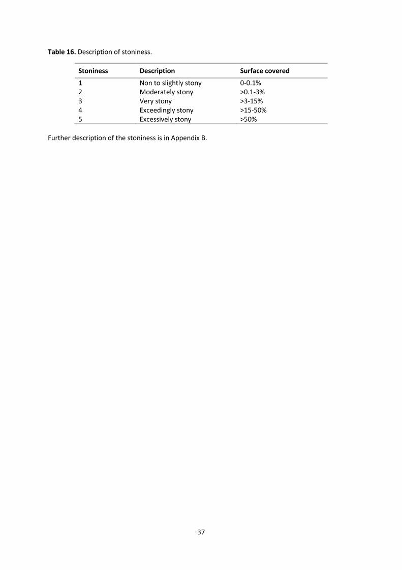
8.2 Appendix B - Description of stoniness. .................................................................................. 70
8.3 Appendix C. Correlation matrixes ......................................................................................... 71
8.4 Appendix D - Field investigation – results table .................................................................... 75
xi
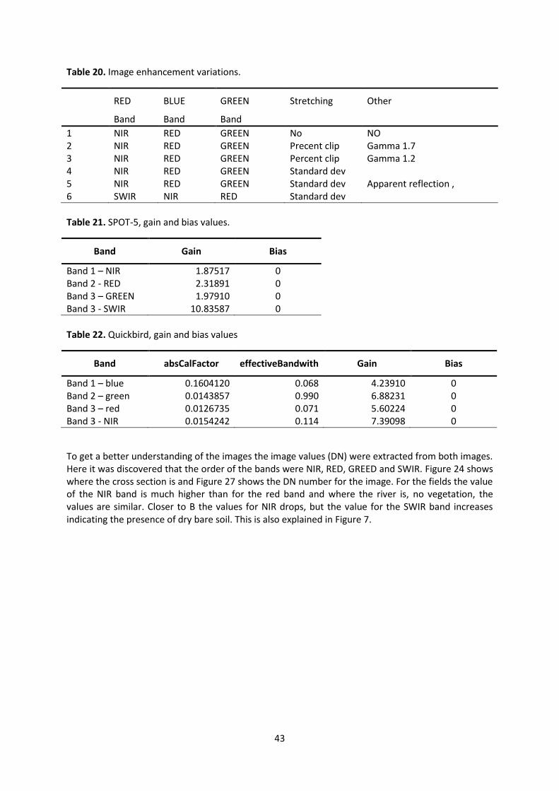
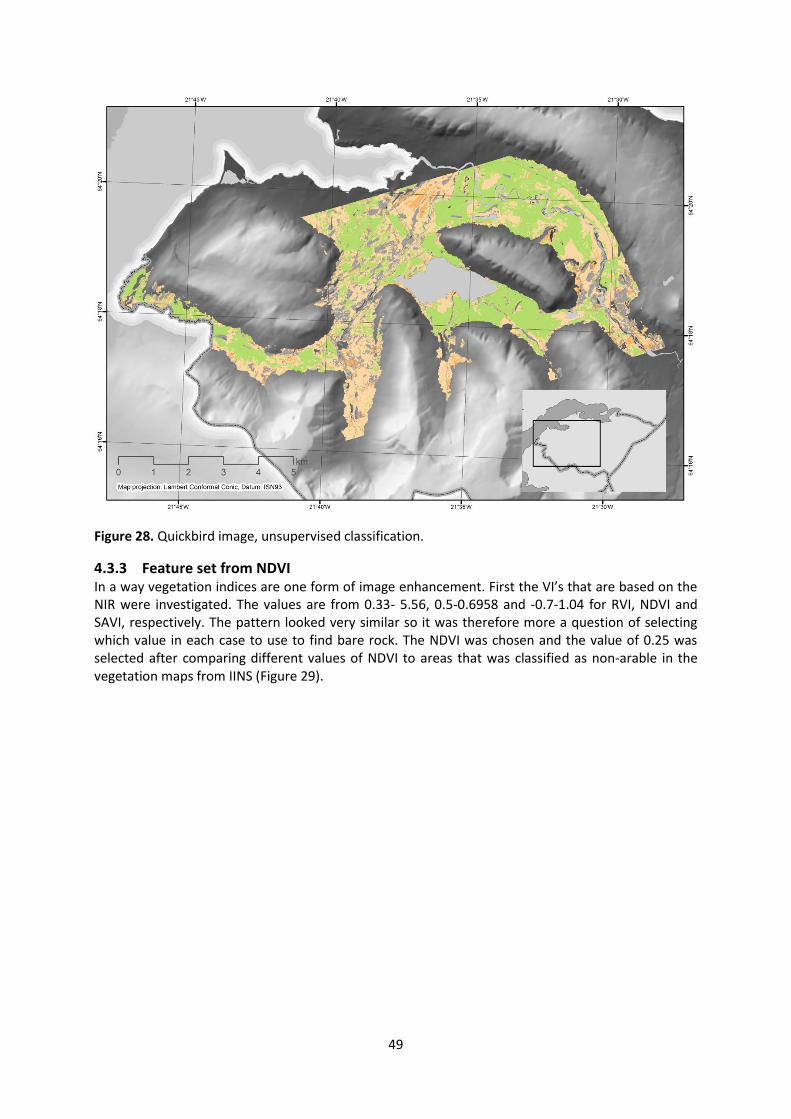
List of Figures Figure 1. Soil map of Iceland (Jóhannesson, 1960). ................................................................................ 3 Figure 2. Soil Map of Iceland (Arnalds and Óskarsson, 2009). ................................................................ 5 Figure 3. Geological of South west part of Iceland (Sæmundsson et al., 2010). .................................... 5 Figure 4. TIN model, nodes and edges left, nodes and facet right (esri, 2012a). ................................... 7 Figure 5. Types of energy levels changes associated with different part of electromagnetic spectrum (Malgorzata, 2010). ................................................................................................................................. 8 Figure 6. Reflectance curve for green vegetation, dry bare soil and water for Spot XS and SPOT Pan. (Looijen, 2004), grey bars spectral range for SPOT-5. ........................................................................... 10 Figure 7. Supervised classification, training samples, histogram and scatterplots ............................... 13 Figure 8. Maximum likelihood (performing the classification) (esri, 2012a). ....................................... 13 Figure 9. Kjósarhreppur overview (Data source Table 7, Projection ISNET 1993 Lambert 1993). ........ 21 Figure 10. SPOT-5 image for Kjósarhreppur. ......................................................................................... 23 Figure 11. Quickbird image for part of Kjósarhreppur. ......................................................................... 23 Figure 12. Overview of where vegetation maps (in draft) are available in Kjósarhreppur. .................. 24 Figure 13. Draft versions of the vegetation maps in Kjósarhreppur (from IIHN). ................................. 26 Figure 14. Workflow for Elevation data, TIN and Slope calculation. ..................................................... 29 Figure 15. Workflow for image classification. ....................................................................................... 33 Figure 16. Instruments in the in-situ testing (Photographs taken by author on field trip 2013). ......... 36 Figure 17. TIN model for Kjósarhreppur with break lines (red). ........................................................... 39 Figure 18. Area below 200 m a.s.l. and with slope from 0-10°. ............................................................ 40 Figure 19. Potential arable land using IFD. ............................................................................................ 41 Figure 20. Potential arable land using IGLUD. ....................................................................................... 42 Figure 21. SPOT-5, with standard deviation stretching of 2.5. ............................................................. 44 Figure 22. Quickbird, with standard deviation stretching of 2.5. ......................................................... 44 Figure 23. Cross section A-B for the SPOT-5 image above and Quickbird below. ................................ 45 Figure 24. Location of cross-section taken for the images, here shown on the SPOT-5 image. ........... 46 Figure 25. SPOT-5 image supervised classification. .............................................................................. 47 Figure 26. SPOT-5 image unsupervised classification. .......................................................................... 48 Figure 27. Quickbird image, supervised classification. ......................................................................... 48 Figure 28. Quickbird image, unsupervised classification. ..................................................................... 49 Figure 29. Vegetation index NDVI for part of the area. ........................................................................ 50 Figure 30. Wetland classified from GNDVI for the area. Total area of wetland is 220 ha. ................... 51 Figure 31. Sample point in in-field observation, classified in the field. ................................................ 52 Figure 32. Potential arable land for Kjósarhreppur. .............................................................................. 54 Figure 33. Future arable land for Kjósarhreppur (Traustason and Gísladóttir, 2009). ......................... 57 Figure 34. Average farm size in hectares divided into arable land and other utilisable agricultural area (UAA) in selected EU countries and Iceland (Eurostat, 2013) ............................................................... 59 Figure 35. Aspects values in the main for direction in the study area. ................................................. 61 Figure 36. Dendrogram ......................................................................................................................... 74
xii
List of Tables Table 1. Further suggested classification of agricultural land (Helgadóttir et al., 2011). ....................... 2 Table 2. Summary of arable land in Iceland from different sources in Iceland. ..................................... 4 Table 3. Error matrix. ............................................................................................................................. 18 Table 4. Spectral range for the SPOT-5 and the Quickbird images. ...................................................... 22 Table 5. Land cover classes for the Icelandic Farmland Database (IFD) showing the full scale classes and the coarser aggregation (Hallsdóttir et al., 2010). ......................................................................... 25 Table 6. Summary of data used. ............................................................................................................ 28 Table 7. Layers used to build the TIN. ................................................................................................... 29 Table 8. Slope values for arable land from different sources. .............................................................. 29 Table 9. Land Capability Classification for classes i-iv (of total vii classes) (Hulme et al., 2002). ......... 30 Table 10. Arable / potential arable land in the IGLUD and IFD land classifications. ............................. 30 Table 11. Reclassification of IFD. ........................................................................................................... 31 Table 12. Reclassification of IGLUD. ...................................................................................................... 31 Table 13. Methods used for overlay analysis for the NDVI-method. .................................................... 34 Table 14. Relationship between minimum map able area and scale. .................................................. 34 Table 15. Overview for the definition of a protected area. .................................................................. 35 Table 16. Description of stoniness. ....................................................................................................... 37 Table 17. Size of test area to evaluate point spacing of elevation points. ............................................ 39 Table 18. Size of area, depending on different reference slope values, in ha and as percentage of the total area of the municipality of Kjósarhreppur (302 km²). .................................................................. 40 Table 19. Arable and potential arable land from IFD and IGLUD, units in ha. ...................................... 41 Table 20. Image enhancement variations. ............................................................................................ 43 Table 21. SPOT-5, gain and bias values. ................................................................................................ 43 Table 22. Quickbird, gain and bias values ............................................................................................. 43 Table 23. Size of area from image classification for SPOT-5 and Quickbird images. ............................ 47 Table 24. Summary of the error matrix, showing overall map accuracy and Kappa estimation. ......... 51 Table 25. Area for resulting features sets from image classifications. ................................................. 52 Table 26. Total area, outside protected area and in protected area. ................................................... 53 Table 27. Continuous potential arable land in Kjósarhreppur. ............................................................. 53 Table 28. Growing Degree Days [D°] for the farm Bær. ........................................................................ 54 Table 29. Comparison of number of image cells in IFD and in the current study. ................................ 57 Table 30. DN values in each band for the present classification........................................................... 58 Table 31. Values of aspect for the Kjósarhreppur area. ........................................................................ 60 Table 32. Database for in-situ testing ................................................................................................... 69 Table 33. IFD_Class: Classification according to the IFD database ....................................................... 69 Table 34. Stoniness: Classification of stoniness (based on(Ontario, accessed 2013, CanSIG, 2013) .... 69 Table 35. Depth: Measured depth in points ......................................................................................... 70 Table 36. Spot-5 Supervised Classification ............................................................................................ 71 Table 37. SPOT-5 Supervised classification - corrected ........................................................................ 71 Table 38. SPOT-5 Unsupervised Classification ...................................................................................... 71 Table 39. SPOT-5 Unsupervised Classification - corrected .................................................................... 72 Table 40. Quickbird Supervised classification ....................................................................................... 72 Table 41. Quickbird Supervised classification - corrected..................................................................... 72 Table 42. Quickbird Unsupervised classification ................................................................................... 73 Table 43. Quickbird Unsupervised classification - corrected ................................................................ 73 Table 44. Edit data from image classification (SPOT-5) ........................................................................ 73 Table 45. SPOT-5 NDVI method, not corrected for fieldwork ............................................................... 74 Table 46. Field investigation results....................................................................................... ..75
xiii
Abbreviations ARVI Atmospherically Resistant Vegetation Index AUI Agricultural University of Iceland LBHÍ Landbúnaðarháskóli Íslands BLUE Blue spectral band CORINE Coordination of Information on the Environment DEM Digital Elevation Model DTM Digital Terrain Model DN Digital Number DVI Difference Vegetation Index EAI Environment Agency of Iceland UST Umhverfisstofnun FAI Farmers Association of Iceland BÍ Bændasamtök Íslands GDD Growing Degrees Days GIS Geographical Information System GNDVI Green Normalized Vegetation Index GPS Global position system GREEN Green spectral band ICERA Icelandic Road Administration VR Vegagerðin IES Institute for Environment and Sustainability IFOV Instantaneous field of view IGLUD Icelandic Geographic Land Use Database IINH Icelandic Institute of Natural History NI Náttúrufræðistofnun Íslands IR Infrared ISOR Icelandic Geosurvey ISOR Íslenskar Orkurannsóknir IFD Icelandic Farm Database Nytjaland IFS Icelandic Forest Service SR Skógrækt ríkisins JRC Joint Research Centre LAS Interchange data format for LiDAR data LiDAR Light Detection and Ranging LPS Leica photogrammetry suite LULUCF Land Use, Land Use Change and Forestry MIR Mid-Infrared NDVI Normalized Difference Vegetation Index NIR Near InfraRed NLSI National Land Survey of Iceland LMÍ Landmælingar Íslands NNFI New national Forest Inventory PAN Panchromatic band PVI Perpendicular Vegetation Index RED Red spectra band REID Red Egde Inflection Point (vegetation index) RMS Root mean square SAVI Soil Adjusted vegetation index SCSI Soil Conservation service of Iceland SPOT Satellite Pour l’Observation de la Terre SWIR Spectral band of SPOT-5 (1.58-1.75 µm) TIN Triangulate irregular network UV Ultraviolet VI Vegetation Index Z Elevation height
xiv
1
1 Introduction Arable land in Iceland is a valuable natural resource that should be preserved. Demand for good arable land in the world is steadily increasing and in some countries like the US, Europe and in many other places it is said that the best arable land is already ploughed (Foley et al., 2011). Globally, agriculture is mainly expanding in the tropics, which is worrisome given that tropical forests are rich reservoirs of biodiversity and provide key ecosystem services. Climate change further accentuates the problem, as more water will be needed for irrigation. With global warming the temperate zone is slowly moving towards the poles and, thus, it might be possible in the future to grow more valuable crops in Iceland than at present. Potential arable land has, however, been gradually taken out of agricultural production over the years and converted into urban areas, such as building sites and roads, and forestry.
Arable land is not an unlimited resource. To be able to protect and preserve it, it is necessary to define arable land and to locate where it is. Arable land is in most cases connected to a farmstead that can either be inhabited or deserted. Most farmsteads in Iceland are below 100 m a.s.l. and it is unusual to find homeland for the farms above 200 m a.s.l. (Snæbjörnsson et al., 2010). There are some exceptions in the north and northeast of the country (around Lake Mývatn). The size of Iceland is about 103,000 km² of which around 25,000 km² is below 200 m a.s.l.. Demand for this land is always increasing.
In the Planning Act from 1998 (No. 400/1998) all municipalities were required to make a general land use plan for urban and rural areas but previously only the urban area needed to be classified. The Act stipulated that an agricultural area included all of the farmstead land used for agriculture. A report should be constructed on the agricultural area and the type of farming undertaken. Only one class for the agricultural area was given, but the municipalities were expected to differentiate between arable land, soil conservation areas and forestry. However, municipalities have addressed this differently. Often agricultural land is all land that is not in other use or the rural land is classified as other land, open area or unpopulated or agricultural area. The municipalities have until recently not had the aim to preserve agricultural land. Only a few of the municipalities report the area of the agricultural land in their general report and therefore the total area of agricultural land is not known. Some of the municipalities have the upper limits of agricultural land in the General Plan, usually along a certain elevation contour in the interval 200-400 m a.s.l..
A new Planning Act (No. 123/2010) came into force on 1 January 2011 and a new Planning Regulation in draft version was issued on 27 October 2010. Municipalities are now required to define both arable land and potential arable land and classify agricultural land according to the type of farming presently being carried out and future plans. Also they should differentiate between cultivated land and potential cultivated land for future use, and between land for food and feed production, forestry and soil conservation. The most demanding requirements in the new Planning Act and accompanying regulation are the definitions of potential agricultural land.
1.1 Aims of the study The aim of the current study was to develop and present a feasible methodology to use for the assessment of potential arable land based on a combination of remotely estimated data and in situ measurements. The final product should be a dataset that can be used for planning purposes and as a tool in strategic planning for land use.
The research questions were:
Can the definition of arable land (1.2) be used to identify arable land with good enough accuracy to use in strategy planning and planning work for land use such as in a General Plan.
Are additional data needed and if so what kind of source data will be needed to add to the precision of the estimates?
2
The Municipality of Kjósarhreppur will be used as a case study. The resulting feature set for arable land will only have a theoretical value and does not include a decision on whether land will be used as arable land. It is up to the local planning authorities to determine priorities of various factors when deciding on land use in accordance with policies, law and guidelines at any particular time, including the preparation of General plans along with landowners (Helgadóttir et al., 2011).
1.2 Definition of arable land In the present study the following definition of arable land, based on Helgadóttir et al., (2011) and Snæbjörnsson et al., (2010), is adopted:
1) Land below 200 m a.s.l. elevation, with the exception that occasional hay fields can be found above this elevation.
2) Soil depth of more than 0.25 m (0.30 m) in order to be workable with a plough as long as stones and gravel are not a hindrance.
3) Drained wetland is one of the most important arable lands. If natural wetlands are to be converted to arable land then the slope should be sufficient to allow for drainage. Wetland bigger than 3 ha is protected.
4) Sandy areas and deltas with the exception of aeolian sands (foksandar) and glacial sands (jökulársandar).
5) Slope should be less than 5-10%, depending on soil type, to hinder erosion. 6) Arable land will be defined up to lakes and rivers, but the protection zone will subsequently
be subtracted. 7) The area must have a minimum continuous area of 3 ha. Drainage ditches within the area do
not affect the requirement of minimum size. 8) Protected areas are excluded.
It is also necessary to take the temperature over the growing season into account. It has been shown that 9.6°C mean temperature for the 130 days from 7 May to 15 September is required for early maturing barley cultivars to reach full maturity in Iceland (Björnsson et al., 2000). Effective total heat sum or Growing Degree Days over the growing season (GDD) (∑T > 0°C, henceforth denoted by °D) decreases about 100°D for each 100m increase in elevation explaining why there is not much arable land over 200 m a.s.l. Further classification for arable land based on Growing Degree Days and soil characteristics have been suggested (Table 1, Helgadóttir et.al, 2011).
Table 1. Further suggested classification of agricultural land (Helgadóttir et al., 2011).
Classification Land cover Growing Degree Days
[D°]
Very good Wetlands and Gleyic andosols >1250
Good Wetlands and Gleyic andosols
Vitric andosols and sand plains
1000-1250
>1250
Possible Vitric andosols and sand plains 1000-1250
3
1.3 Previous estimates of arable land There is no information available about the exact area of potential arable land in Iceland. There is better information available on land that has already been cultivated. According to Helgadóttir and Hermannson (2003) about 1,200 km² are now under cultivation of which 90% are hayfields (15% are leys and 75% are permanent). Around 10% of this area is cultivated each year.
Several attempts have been made to estimate the potential arable land in Iceland. In his report, The Soils of Iceland, Björn Jóhannesson classified the soil according to agricultural requirements on the scale 1:500,000 (Jóhannesson, 1960). This classification used 0.15 m depth of soil but neither the variability nor continuity is known (Figure 1). Jónatan Hermannsson (personal communication) has used these maps to roughly estimate the area of potential arable land to be in the order of 15,000 km².
Figure 1. Soil map of Iceland (Jóhannesson, 1960).
In 1961 the National Land Survey of Iceland (NLSI) published estimates on vegetation cover in Iceland based on their maps at the 1:100,000 scale. The total surface area was classified into vegetated land, water, desert and glaciers depending on height above sea level. Vegetated land was 13,718 km² and arable desert 9,112 km². It was estimated that it would be possible to convert about 5,000 km² of the desert to arable land, but about 20% of the potential arable land would be needed for construction, roads etc., reducing the estimate to about 15,000 km². This estimate has since been used in governmental data for arable land below 200 m a.s.l. (Snæbjörnsson et al., 2010).
By restricting this definition to land that could be ploughed and used for the production of barley (see above) Áslaug Helgadóttir and Jónatan Hermannsson estimated that there were about 6,000 km² of such good arable land available (Snæbjörnsson et al., 2010).
Traustason and Gísladóttir (2009) were the first to use Geographic Information Systems (GIS) to estimate future arable land. They based their estimate on the land cover classification in the Icelandic Farmland Database (IFD, Nytjaland, see later) and / or from the European land cover project, Coordination of Information on the Environment (CORINE), using the following assumptions:
4
The area must be restricted to the categories grassland, richly or poorly vegetated land or semi-wetland.
Be outside protected areas around roads and urban areas, but not further away than 2 km from main roads.
Slope < 10° and elevation < 200 m a.s.l.
Protected areas are excluded. This resulted in 6,150 km² of potential arable land, or about 25% of the land below the 200 m a.s.l. line. Sveinsson and Hermansson (2010) estimated the potential arable land with assistance from local agricultural advisors, and using estimates from the Icelandic Biomass Company (Björnsson, 2007) to be only 420 km². This estimate was based on the assumption that minimum size of continuous land available was at least 30 ha. In the CORINE-project, agricultural land is one of the 5 main classes, and it is subdivided into 11 surface types (Árnason and Matthíasson, 2009). Only 3 of these 11 surface types are found in Iceland; pastures, non-irrigated arable land and complex Cultivation Patterns. According to the CORINE classification agricultural land in Iceland is 2.4% (~2,500 km²) and most of it is pastures (97%) (Árnason and Matthíasson, 2009). The map scale for the CORINE project is 1:100,000 and the smallest cartographic unit is 25 ha. The results of different estimates of arable and/or agricultural land are shown in Table 2. These have been based on different scales, minimum mapping units and minimum size of arable land.
Table 2. Summary of arable land in Iceland from different sources in Iceland.
Source Size of arable land
[km²]
Jóhannesson (1960) 15,000 NLSI 1961 15,000 Helgadóttir and Hermannsson (2003) 6,000 Traustason and Gísladóttir (2009) 6,150 Árnason and Matthíasson, (2009) 2,500 Sveinsson and Hermannsson (2010) 420
A new Icelandic soil map was published in 2009 (Arnalds and Óskarsson, 2009). This map is in digital format at the 1:250,000 scale (Figure 2). Because of its small scale its primary aim is to give an overview of the soil types in an international context such as the Soil Atlas of Europe (Jones et al., 2005) and the Soil Atlas of the Northern Circumpolar Region (Jones et al., 2010) rather than for use on a detailed scale.
The Icelandic Geosurvey (ISOR) has also published a geological map for the South-West part of Iceland (Figure 3) (Sæmundsson et al., 2010).
5
Figure 2. Soil Map of Iceland (Arnalds and Óskarsson, 2009).
Figure 3. Geological of South west part of Iceland (Sæmundsson et al., 2010).
6
7
2 Background
2.1 Elevation model The definition of arable and potential arable land depends, among other things, on the properties of the surface, i.e. the elevation and the slope. The surface is a continuous phenomenon and, hence, a digital terrain model (DTM) or a digital elevation model (DEM), which has a value in every point across the area, would be applicable. To model the surface it would be necessary to store an infinite number of observation points. However, that is impossible so a surface model is made of a limited number of observation points (height points). The resolution of the DEM is determined by the frequency of the points. It is created from series of regular or irregular data points. It can be derived from different sources but for surface elevation it is usually made from either contours or spot heights. It can also be made from stereoscopic interpretation from aerial photographs taken of the same area in the same patch of ground but with slightly different angle. This method relies on the calculation for elevation based on the parallax displacement between the same points on both images. Light Detection and Ranging (LiDAR) is other kind of remotely sensed data that have been developed that directly measure elevation using laser scanning sensors (Heywood et al., 2006). LiDAR technology offerers advantages over traditional methods for represetning a terrain surface. The advantages refer to accuracy resolution and cost. One of the most attractive characteristics of LiDAR is its very high verticla accuracy (Vaze and Teng, 2007).
The surface models have different data storage formats, such as raster, Triangulate Irregular Network (TIN), terrain or LAS (interchange format for lidar data). For a surface model, a TIN will be constructed. Here it will be made up of irregular height points, red points similar to that shown in Figure 4. The surface data structure is made of triangular facets or a triangular network defined by nodes and edges. The terrain height is derived from the measured points that are used as initial nodes in the triangulation. The shape of the TIN surface is controlled by the triangulation of these spot elevations. The spot elevation can be irregularly distributed to accommodate an area of height variability in the surface and their values and exact position are retained as nodes in the TIN. Additional features can be incorporated into the TIN model. This includes breaks of slopes such as ridges, troughs and cliff edges/bases. Water features like lakes and ocean can also be incorporated as flat areas with surface water. Rivers and streams can be defined as trough lines.
Figure 4. TIN model, nodes and edges left, nodes and facet right (esri, 2012a).
The main advantage of the TIN data model is the efficiency of data storage because only a minimum number of significant points is needed to produce a surface. Since a TIN is made up of an irregular network there can be many points in mountainous areas and fewer where the landscape is flat. If a height point can be interpolated from its neighbour’s then the point is not considered to be ‘surface significant’ and is dropped from the TIN model. Only those points that cannot be interpolated from their neighbours are considered ‘surface significant’ and are used as TIN vertices (Heywood et al., 2006).
ArcGIS desktop uses Delaunay triangulation and it is possible to choose between conforming or constrained approaches, even though the conforming Delaunay triangulation is recommended (esri,
8
2012b). This method is more likely to give fewer long, thin triangles which are undesirable for surface analysis. Further, natural neighbours and Thiessen (Voronoi) polygons generation is only possible with this method. Here break lines are densified with Steiner points to ensure that the TIN remains Delaunay conforming. A constrained Delaunay triangulation can be considered when it is necessary to define certain edges that cannot be modified by the triangulator. It is also useful for minimizing the size of the TIN, since the break lines are not densified and thus have fewer nodes and edges.
2.2 Remote sensing There are a number of different definitions of remote sensing but all of them have in common that information about characteristics, such as the physical, chemical, biological properties of the Earth surface, is obtained by a device that is not in contact with the object being measured. This information is obtained through measurements of the electromagnetic radiation that is reflected, emitted or scattered from the object. Remote sensed data are acquired both by using satellite remote sensing and aerial photography, as well as radar.
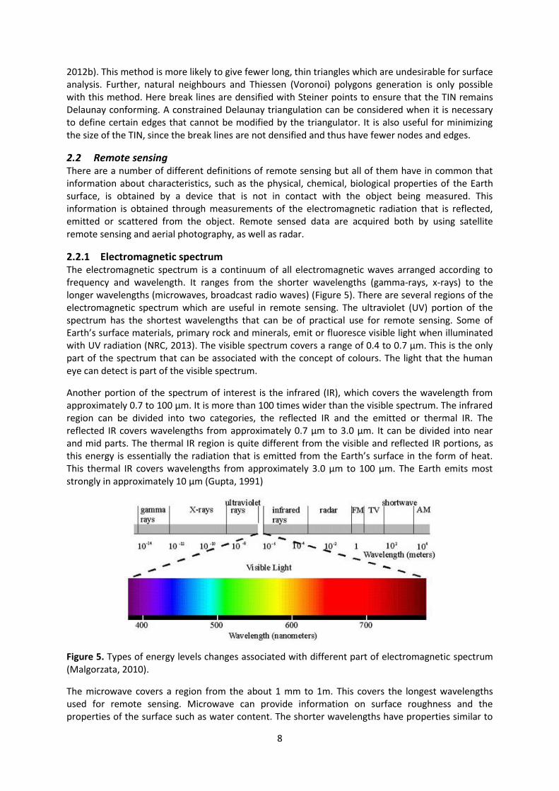
2.2.1 Electromagnetic spectrum The electromagnetic spectrum is a continuum of all electromagnetic waves arranged according to frequency and wavelength. It ranges from the shorter wavelengths (gamma-rays, x-rays) to the longer wavelengths (microwaves, broadcast radio waves) (Figure 5). There are several regions of the electromagnetic spectrum which are useful in remote sensing. The ultraviolet (UV) portion of the spectrum has the shortest wavelengths that can be of practical use for remote sensing. Some of Earth’s surface materials, primary rock and minerals, emit or fluoresce visible light when illuminated with UV radiation (NRC, 2013). The visible spectrum covers a range of 0.4 to 0.7 µm. This is the only part of the spectrum that can be associated with the concept of colours. The light that the human eye can detect is part of the visible spectrum.
Another portion of the spectrum of interest is the infrared (IR), which covers the wavelength from approximately 0.7 to 100 µm. It is more than 100 times wider than the visible spectrum. The infrared region can be divided into two categories, the reflected IR and the emitted or thermal IR. The reflected IR covers wavelengths from approximately 0.7 µm to 3.0 µm. It can be divided into near and mid parts. The thermal IR region is quite different from the visible and reflected IR portions, as this energy is essentially the radiation that is emitted from the Earth’s surface in the form of heat. This thermal IR covers wavelengths from approximately 3.0 µm to 100 µm. The Earth emits most strongly in approximately 10 µm (Gupta, 1991)
Figure 5. Types of energy levels changes associated with different part of electromagnetic spectrum (Malgorzata, 2010).
The microwave covers a region from the about 1 mm to 1m. This covers the longest wavelengths used for remote sensing. Microwave can provide information on surface roughness and the properties of the surface such as water content. The shorter wavelengths have properties similar to
9
the thermal infrared region while the longer wavelengths approach the wavelengths used for radio broadcasts (NRC, 2013, Janssen and Huurneman, 2001).
The energy recorded by the remote sensing system undergoes fundamental interactions with the atmosphere and earth surface. The interaction with the atmosphere is absorption, transmission and scattering.
2.2.2 Interaction with the earth surface When the electromagnetic energy reaches the earth surface three fundamental energy interactions are possible, i.e. reflection, absorption and / or transmission. The proportion of energy that is reflected, absorbed and transmitted varies for different earth features, depending on their material type and condition, making it possible to distinguish between different features on the image. These interactions are also dependent on the wavelength, which means that even with given feature types the proportion of reflected, absorbed and transmitted energy will vary at different wavelengths. Features can therefore not be distinguishable in one spectral range and be very different in another. The geometric manner in which an object reflects energy is also of importance. There are two types of reflectance, specular and diffuse. The category that describes any given surface is dictated by the surface’s roughness in comparison to the wavelength of the energy being sensed. When the wavelength of incident energy is much smaller than the surface height variations or the particle size, that make up the surface, the reflection from the surface is diffuse. In remote sensing it is important to measure the diffuse reflectance properties of terrain feature because it contains spectral information on the colour of the reflection surface (Lillesand, 2008).
The reflectance characteristics of features on the Earth’s surface may be quantified by measuring the portion of incident energy that is reflected. This is measured as a function of wavelength and is called spectral reflectance (p 13). Experience has shown that many Earth surface features of interest can be identified, mapped and studied on the bases of their spectral characteristics. Experience has also shown that some features of interests cannot be spectrally separated (Lillesand et al., 2008).
2.2.3 Resolution of remote sensed data Resolution is the key physical characteristic of remote sensing data. There are four elements of resolutions:
spatial resolution
spectral resolution
radiometric resolution
temporal resolution
Spatial resolution refers to the smallest size of an object or linear separation between two objects that can be resolved on the ground. In digital image, the resolution is limited by the pixel size, i.e. the smaller resolvable object cannot be smaller than the pixel size. The intrinsic resolution of an imaging system is determined primarily by the instantaneous field of view (IFOV) of the sensor, which is a measure of the ground area viewed by a single detector element in a given instant in time. However, this intrinsic resolution can often be degraded by other factors which introduce blurring of the image, such as improper focusing, atmospheric scattering and target motion. The pixel size is determined by the sampling distance (Liew, 2001).
Spectral resolution is the number and dimension (size) of a specific wavelength interval (referred to as bands or channels) in the electromagnetic spectrum to which a remote sensing instrument is sensitive. For example SPOT-5 has five bands: 0.48 – 0.71 µm (panchromatic band PAN), 0.5 – 0.59 µm (green band, GREEN), 0.61 – 0.68 µm (red band, RED), 0.78 – 0.89 µm (near-infrared band, NIR) and 1.58 – 1.75 µm (shortwave-infrared band SWIR). Careful selection of the spectral bands might improve the probability that the desired information will be extracted from the remote sensor data
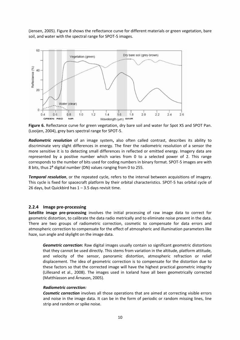
10
(Jensen, 2005). Figure 8 shows the reflectance curve for different materials or green vegetation, bare soil, and water with the spectral range for SPOT-5 images.
Figure 6. Reflectance curve for green vegetation, dry bare soil and water for Spot XS and SPOT Pan. (Looijen, 2004), grey bars spectral range for SPOT-5.
Radiometric resolution of an image system, also often called contrast, describes its ability to discriminate very slight differences in energy. The finer the radiometric resolution of a sensor the more sensitive it is to detecting small differences in reflected or emitted energy. Imagery data are represented by a positive number which varies from 0 to a selected power of 2. This range corresponds to the number of bits used for coding numbers in binary format. SPOT-5 images are with 8 bits, thus 2⁸ digital number (DN) values ranging from 0 to 255.
Temporal resolution, or the repeated cycle, refers to the interval between acquisitions of imagery. This cycle is fixed for spacecraft platform by their orbital characteristics. SPOT-5 has orbital cycle of 26 days, but Quickbird has 1 – 3.5 days revisit time.
2.2.4 Image pre-processing Satellite image pre-processing involves the initial processing of raw image data to correct for geometric distortion, to calibrate the data radio metrically and to eliminate noise present in the data. There are two groups of radiometric correction, cosmetic to compensate for data errors and atmospheric correction to compensate for the effect of atmospheric and illumination parameters like haze, sun angle and skylight on the image data.
Geometric correction: Raw digital images usually contain so significant geometric distortions that they cannot be used directly. This stems from variation in the altitude, platform attitude, and velocity of the sensor, panoramic distortion, atmospheric refraction or relief displacement. The idea of geometric correction is to compensate for the distortion due to these factors so that the corrected image will have the highest practical geometric integrity (Lillesand et al., 2008). The images used in Iceland have all been geometrically corrected (Matthíasson and Árnason, 2005).
Radiometric correction:
Cosmetic correction involves all those operations that are aimed at correcting visible errors and noise in the image data. It can be in the form of periodic or random missing lines, line strip and random or spike noise.
11
Atmospheric correction: All reflected and emitted radiation leaving the Earth’s surface are attenuated mainly due to absorption and scattering by constituents in the atmosphere. The atmospheric induced distortions occur twice in the case of sunlight reflection and once in the case of emitted radiation. These distortions are wavelength dependent and can be reduced by applying atmospheric correction techniques. These corrections are related to the influence of haze, sun angle and skylight.
Haze compensation procedures are designed to minimize the influence of path radiance effects. This is based on the assumption that the infrared bands are essentially free of atmospheric effects and in these bands black bodies, such as large clear water and shadow zone will have zero DN-value. The DN-values in other bands for the corresponding pixels can be attributed to haze and should be subtracted from all pixels of the corresponding band.
Sun angle correction. The position of the sun relative to the earth changes depending on the time of day of the year. In the northern hemisphere, the solar elevation angle is smaller in winter than in summer. As a result, the image data of different seasons are acquired under different solar illumination. Sun angle correction becomes more important when one wants to generate mosaics taken at different times or perform change detection studies.
Skylight correction requires additional information that cannot be extracted from the image data. This is because of scattered light reaching the sensor after being reflected from the Earth’s surface constitutes the skylight or sky irradiance. This also reduces contrast in the image.
Satellite image enhancement is used to ease the visual interpretation and understanding of the imagery. Usually this involves techniques for increasing the visual contrast between the features in order to increase the amount of information that can be visually interpreted from the data (NRC, 2013).
2.3 Image classification Interpretation and analysis of remote sensing imagery involves the identification and / or measuring various targets in an image in order to extract useful information about them. The resulting raster from image classification can be used to create thematic maps. Now it is more common to perform digital processing and analysis, but visual analysis is always used with it, like tone, shape, size, pattern texture shadows and association. Depending on the interaction between the analyst and the computer during classification there are two types of classification: supervised and unsupervised (esri, 2012a).
Unsupervised classification finds spectral classes (or clusters) in a multiband image without the analyst’s interference. Spectral classes are grouped first, based on the numerical information in the data and then matched by the analyst to information classes. Cluster algorithms are used to determine the natural (statistical) grouping. The analyst specifies how many groups or clusters are to be looked for and the number of iterations. In addition the analyst may also specify parameters related to the separation distance among the clusters and the variation within each cluster, i.e. the minimum class size and sample interval.
The iso (iterative self-organizing) clustering method uses a process where all samples are assigned to existing cluster centres during iteration and new means are recalculated for each class. The optimal number of classes to specify is usually unknown. The number of iterations should be large enough to ensure that the migration of cells from one cluster to another is minimal, and therefore becomes stable. Clusters consisting of fewer cells than the specified minimum class size value are eliminated at the end of the iterations. The value entered for the sample interval, indicating one cell out of every n-by n block of cells, is used in the cluster calculation (esri, 2012a)
12
Supervised classification uses spectral signatures obtained from training samples to classify an image. The analyst identifies in the imagery homogeneous representative samples of the different surface cover types (information classes) of interest. These samples are referred to as training areas. The selection of appropriate training areas is based on the analyst’s familiarity with the geographical area and knowledge of the actual surface cover types present in the image. Thus, the analyst is supervising the categorization of a set of specific classes. The numerical information in all spectral bands for the pixels comprising these areas is used to train the computer to recognize spectrally similar areas for each class. The computer uses a special program or algorithm to determine the numerical signatures for each training class. Once the computer has determined the signature for each class, each pixel in the image is compared to these signatures and labelled as the class it most closely resembles digitally.
Supervised classification has three basic steps, training stage, classification stage and output stage.
Training stage: The analyst identifies representative training areas and develops a numerical description of the spectral attributes of each land cover type of interest in the scene.
Classification stage: Each pixel in the image data set is categorised into land cover class it most closely resembles. If the pixel is insufficiently similar to any training data set it is usually labelled unknown. The category label assigned to each pixel in this process is then recorded in the corresponding cell of an interpreted data set (output image). Thus the multidimensional image matrix is used to develop a corresponding matrix of interpreted land cover category types.
The classification stage is the heart of the supervised classification process. During this stage the spectral pattern in the image data is evaluated in the computer using predefined decision rules to determine each pixel. Here certain knowledge is needed about the study area or samples of each class. The goal is to assign each cell in a study area to a class or category.
Multivariate statistics are calculated from the training samples to establish the relationships within and between the classes. A class corresponds to a meaningful grouping of locations like water bodies or fields. Each location is characterized by a set of vector values for each variable or band entered in the analysis. Each location can be visualized as a point in a multidimensional space whose axes correspond to the variable presented by each input band. A class or cluster is a grouping of points in this multidimensional attribute space. Two locations belong to the same class or cluster if their attributes (vector of bands) are similar (esri, 2012a).
To evaluate the training samples and make sure that they are distinguishable their spectral characteristics have to be checked and compared. This is done by using histogram and scatterplots as shown in Figure 7. Here in this figure this is for potential land / wetland with somekind of a citron yellow color, non-arable land as brown, field as dark violet, and water as green
Here maximum likelihood classification is used, and it is based on two principles:
Cells in each class sample in the multidimensional space is being normally distributed Bayes’ theorem of decision making The tool considers both the variances and covariance of the class signature when assigning each cell to one of the classes represented. With the assumption that the distribution of a class sample is normal, a class can be characterized by the mean vector and covariance matrix. Given these two characteristics for each cell value, the statistical probability is computed for each class to determine the membership of the cells to the class. But the cells are rarely homogeneous. It is a possibility that a cell belongs to two classes that overlap each other (Figure 10). The maximum likelihood classifier calculates for each class the probability of the cell belonging to that class given its attributes values. The cell is assigned to the class with the highest probability (esri, 2012a).
13
Figure 7. Supervised classification, training samples, histogram and scatterplots
The assumption for the maximum likelihood classifier to work accurately is as follows:
The data for each band should be normally distributed Each class should have a normal distribution in multivariate attribute space The prior probabilities of the classes must be equal
Figure 8. Maximum likelihood (performing the classification) (esri, 2012a).
Output stage: This is the final stage in the image classification. Here the aim is to produce output from the classification that clearly shows the interpreted information to the end user. The results are
14
digital in character and the results may be used in different format, hardcopy graphic products like thematic maps, table area statistics and digital data files (Lillesand et al., 2008).
Post classification methods: Classified data often manifest a salt-and-pepper appearance due to the inherent spectral variability encountered by a classifier when applied on a pixel-by pixel bases. Post classification processing refers to the process of removing the noise and improving the quality of the classified output. These are methods like majority filter to remove isolated pixels or noise from the classified output, smoothing the ragged class boundaries and clumps in the classes and removing small isolated regions.
2.4 Vegetation indices Vegetation indices (VI) have been used in remote sensing for many decades. Over 50 different VIs have been developed in recent years (Ozbakir and Bannari, 2008). A VI can be calculated by taking the ratio between different spectral bands, and by forming linear combinations of spectral band data. It can be calculated from sensor voltage outputs (V), radiance values (L), reflectance values (ρ) and satellite digital numbers (DN). It is possible to use any of these (V, L, ρ) but each will yield a different VI value for the same surface conditions. View and solar angle may affect data from each spectral band differently. Soil background has a major influence on it. VI calculated from data obtained from aircraft or spacecraft-based sensors are affected by the intervening atmosphere (Jackson and Huete, 1991).
The first VI was used to show spectral properties at different stages of growth and senescence. Then VIs were developed to take background effects such as that caused in areas in which the soil response dominates (SAVI, PVI) over vegetation. The third type of VIs were then developed to compensate for the effects of atmospheric distortion (ARVI). In recent years spectral VIs have been developed for applications other than vegetation health, like image classification and to separate vegetation from non-vegetated areas (Campell, 1996).
VIs have been grouped from two, three, or four different groups (Jackson and Huete, 1991; Silleos et al., 2006; Mróz and Sobieraj, 2004). All these indices use some kind of formulation between the near infrared (NIR) and the RED band. Then there are other indices that use other bands like the GREEN or the mid infrared band (MIR, SWIR). The groups of VIs are:
Slope based indices Distance based indices Orthogonal transformation Red Edge Inflection Point (REIP) Other VIs Slope based VI’s are combinations of the visible red and the NIR bands and are widely used to generate VI’s. The values indicate both the state and abundance of green vegetation cover and biomass (Silleos et al., 2006). Distance based VIs are derived from the Perpendicular Vegetation Index (PVI). The objective of these VIs is to cancel the effect of soil brightness in cases where vegetation is sparse and pixels contain a mixture of green vegetation and soil background. This is based on the soil line concept. The soil line represents a description of the typical signature of soil in a RED/NIR bi-spectral plot and is obtained by linear regression for a sample of bares soil pixels (Silleos et al., 2006). Orthogonal based VI’s have been approached through orthogonal transformation techniques. These techniques express vegetation through the development of the second component (Silleos et al., 2006).
15
Red Edge Inflection Point (REIP). VIs based on waveform analysis techniques. They make use of the Gaussian, polynomial and Lagrangian models, respectively (Mróz and Sobieraj, 2004).
Other VI’s use other bands than the RED and the NIR band. This is either the GREEN band or the SWIR band.
Here the intention is to look at VIs to classify potential agricultural land. According to Joshi (2011) various techniques have been developed to map vegetation with varying accuracy and cost. The simplest one to is use vegetation indices as they are easy to understand and calculate. He compared the Normalized Differential Vegetation Index (NDVI), TDVI and Soil Adjusted Vegetation Index (SAVI) and concluded that the NDVI gave the best results. In the studies on habitat types in Iceland Hreinsdóttir et al. (2006) compared RVI, DVI, NDVI, SAVI and GNDVI and concluded that the GNDVI gave best results. Ray (1994) recommends the following indices: NDVI (best known and most used), PVI, SAVI and MSAVI2. The Normalized Difference Water Index (NDWI) has also successfully been used to delineate surface water and is often used for soil moisture mapping (McFeeters, 1996). RVI - Ratio Vegetation Index (simple ratio index) The RVI, Eq. 1, is a simple ration-based index or slope based index. It is one of the first vegetation indices and was first described by (Jordan, 1969). This is one of the most widely calculated vegetation index (Ray, 1994). It is sensitive to the amount of vegetation. RVI has the ability to distinguish the soil and vegetation but not in shaded areas. Hence, RVI does not give proper information when the reflected wavelengths are being affected due to topography, atmosphere or shadows:
(1)
The value of this index ranges from 0 to more than 30 or even infinity. The common range for green vegetation is 2 to 8. If both the RED and NIR bands have the same or similar reflectance the RVI is 1 or close to 1, which is often the case for bare soil.
NDVI - Normalized Difference Vegetation Index. NDVI, Eq. 2, is one of the most common vegetation indices. It was ascribed to (Rouse et al., 1973), but the concept of a normalized index was first presented by Kriegler et al. (1969)(in) (Ray, 1994). It is expressed as the difference between the near infrared band and the red bands normalized by the sum of these bands. It minimizes the topographic effects while producing liner effects:
(2)
The NDVI is preferred to the simple index (global vegetation monitoring) because it helps compensate for changing illumination conditions, surface slope, aspect and other extraneous factors (Lillesand et al., 2008). The value ranges from -1 to 1, where 0 is no vegetation, and negative values non-vegetated areas. The common range for green vegetation is 0.2 to 0.8.
SAVI – Soil Adjusted Vegetation Index The SAVI, Eq 3, was proposed by Huete (1988). It attempts to be a hybrid between the ratio-based indices and the perpendicular indices. It is aimed at minimizing the soil influence on vegetation quantification by introducing the soil adjustment factor L. For high vegetation cover the value of L is 0.0 (or 0.25), and for low vegetation cover – 1.0. For intermediate vegetation L = 0.5, and this value is most widely used. It incorporates a constant soil adjustment factor L into the denominator of the NDVI equation:
(3)
16
When L = 0, it is the same as NDVI, Eq. 2. In the study by Dematte et al. (2009), the same pixel was evaluated by a vegetation index for SAVI. When the value for SAVI was zero it was considered to be an indicator of bare soil. The value of L was then 0.5, resulting in the constant 0.5 and 1.5 in Eq. 3. This is referred to as the gain and off-set coefficients.
GNDVI – Green Normalized Difference Vegetation Index The GNDVI, Eq. 4, is similar to the NDVI but uses the green band instead of the red band:
(4)
GNDVI may be a more reliable indicator of crop condition (Lillesand et al., 2008). This index has shown best correlation to different habitat types in Iceland (Hreinsdóttir et al., 2006).
NDWI – Normalized Difference Water Index There are two different definitions of the NDWI, Eq 5 and Eq 6. One, Eq. 5, was introduced by (Gao, 1996) and is “proposed for remote sensing of liquid water from space”. It was used to estimate water content of vegetation canopy. It is defined similarly to the NDVI index but uses the reflectance 0.86 and 1.24 µm:
(5)
or
(6)
NDWI is sensitive to changes in liquid water content of vegetation canopies. It is less sensitive to atmospheric effects then NDVI. It does not completely remove background soil reflectance as NDVI. It should be considered as an independent vegetation index and it is complementary rather than a substitute for NDVI. Common values for 100% vegetation cover is 0.06, for soil -0.022, grass 0.084 and crop 0.215 (Gao, 1996). Values of NDWI can be negative for bare soil.
The other one, Eq. 7, was introduced by McFeeters (1996) and it was a new method that was developed to delineate open water features and enhance their presence in remotely-sensed digital imagery:
(7)
The selection of these wavelengths was done to:
1) Maximize the typical reflectance of water features by using green light wavelengths 2) Minimize the low reflectance of NIR by water features 3) Take advantage of the high reflectance of NIR terrestrial vegetation and soil features
For the NDWI index, water features have positive values whereas soil and terrestrial vegetation features have zero or negative values. This is the same as GNDVI index with reversed sign.
2.5 Map Accuracy The image classification is not finished until the map accuracy has been assessed. There are three basic elements for the accuracy assessment; the sampling data, the response design and the error estimation. The sampling data is needed for the comparison with the classified data. In this evaluation, attributes for the classified data (map data) are compared with the attribute of the
17
sample data (ground truth) in each location. This comparison is used to prepare an error or confusion matrix. For both of these it is necessary to look into a sample design and the calculation and setup of the error matrix, respectively.
2.5.1 Sampling design To make the map assessment it would be best to collect sample points in all locations. But that is impossible. So the aim of the sample design is to sample points with limited number of points at carefully chosen locations to get representative information of the area. There are many factors that have to be taken into account like:
Number of sample points
Sample size
Sample distribution
Sampling units
Besides there are other factors like time and money, and the place has to be reachable. The position of the sample points is of great importance and the area covered should be larger than the error in positioning. Other factors that influence the size of the sample area are the cell size of the raster in the map and the minimum size of an object in the map (lecture notes). Number of sample points: The more sampling points one uses (up to some threshold where one is oversampling), the better the estimate. The rule of thumb is 30 points for each class (Map Accuracy Assessment), but it has also been stated that the number of samples within each category of interest ought to be at least 50 (Brogaard and Ólafsdóttir, 1997, Lillesand et al., 2008). In the case of a very large area (more than 400 ha) or if there are large numbers of vegetation or land use cover classes the number of samples should be increased to 75 or 100 samples per category (Lillesand and Kiefer, 1994). Also the number of samples might be adjusted to the importance of the categories or variability within the categories. Too small number of sample point increases the risk of either Type I Error, rejecting a correct map or Type II Error accepting a bad map (LUMA-GIS, 2004). Sample size is estimated from the formula in Eq. 8 (Brogaard and Ólafsdóttir, 1997; Klinkenberg, 2004): (8) where: A: is the minimum sample site dimension P: is the image pixel dimension L: is the estimated location accuracy in number of pixel Sample distribution: The most important factor in the sampling design is the distribution of the sample points. Here the aim is to collect sample points that represent the map area. For statistical purposes random sampling is preferred. In spatial terms, a random sample is one in which each location has the same chance of being chosen, and the choice of one location in no way changes the probability of another location to complete the sampling (Robinson et al., 1995, Robinson, 1995). The most common sample schemes are:
Simple random sampling. Here all locations have the same chance of being selected. This can result in many points and is thus time consuming and inefficient. This relates to the probability theory where the distribution of values can give us information of the distribution of the parent population. But with bad luck it is possible that in some places the sample points are
18
unevenly distributed or too dense at some points and too few points at others. Simple random sampling tends to under sample small but potentially important areas (Lillesand et al., 2008) Systematic sampling. For this scheme the sample points are collected in a regular pattern. Here the locations do not have the same chance of being selected. The advantage is that the entire area will be covered, but the disadvantage is that each unit in the population does not have equal chance of being in the selected sample (Brogaard and Ólafsdóttir, 1997). The interval in the pattern can be the same or be variable. When little is known about the area uniform sample distribution is preferred to random distribution. By this method it is less likely to miss major distribution but at the same time minor differences can easily be missed (Robinson, 1995). Systematic sampling should be used with caution because it may overestimate the population parameters (Jensen, 2005) Stratified random sampling. In this type of sampling scheme the area is first divided into sub-areas called strata. Here the location points do not have the same chance of selection. The question is then how to divide the area into strata, homogenous sub areas, or systematic grid (random systematic), land cover classes or vegetation types. But here usually few points are needed for the sample data (Robinson et al., 1995).
There are also other sampling arrangements like transect sampling and road sampling that are both fast but not representative. Then there is cluster sampling where many points are taken within a small distance (cluster) and then there are some clusters in the area. In general the recommendation is either random or stratified random sampling with 50 point for each class (LUMA-GIS, 2004).
2.5.2 Reference data The map data have to be prepared with other data. Most often the data are compared with reality, i.e. ground truth points collected in the field, but it can also be compared with another map.
2.5.3 Error matrix Comparison between the map data and the reference data (or ground truth data) is done by establishing an error matrix or confusion matrix as in Table 3. The map data are in the rows while the ground truth data are in the columns. This is a type of an uncertainty matrix. In the diagonals there is an agreement between the map data and the ground truth data. In other cells there is mismatch in the classification. For example, if a map point is classified as A but in the ground it is classified as C it appears as AC in the cell. Likewise if a ground truth is classified as A but is in the map like C it is in the cell CA (Foody, 2002, Congalton, 1991).
Table 3. Error matrix.
Ground truth
A B C D Σ
Map
dat
a A
B C
D
Σ
There are various measures to decribe the accuracy from the error matrix.
19
Overall accuracy or Map accuracy, Eq. 9, is the ratio of total numbers of correctly (summation of the diagonal) and total number of samples classified:
∑
(9)
User accuracy or object accuracy, Eq. 10, compares the map data with field data, or the probability that a randomly selected point is classified as A in the field is also classified as A on the map:
(10)
Producer accuracy, Eq. 11, is the other way around compared to the user accuracy. It is the probability that a point that is classified as A in the field is classified as A on the map:
(11)
Mean Accuracy, Eq. 12, is a combination of user accuracy and producer accuracy and always falls in between these two:
(12)
Areal difference, Eq.13, is used to compare the different classes on the map with ground truth and is always related to the ground truth area. It is always divided by . When the map is over classified then the map contains more points for certain classes and the verification data. Under classification is the reverse:
(13)
Kappa statistics or coefficient of agreement, Eq 14, is a widely used measure for map accuracy. The overall Kappa gives information on the quality of the map, whether it is equal or above random chance as well as quantitative value of this agreement.
The Kappa coefficient is calculated as:
(14)
Or
∑
∑
∑
(15)
where r: number of rows in the error matrix the number of observation in row i and column i (on the major diagonal) total observations in row i (shown as marginal total to right of the matrix) total observations in column i (shown as marginal total at the bottom of the matrix) N: total number of observations included in the matrix
20
And the kappa values are: -1: map does not correspond to ground truth 0: random agreement
1: the map and the ground truth have the same points
21
3 Materials and Methods
3.1 Study area The present case study is limited to Kjósarhreppur Municipality. It is located in the south west corner of Iceland, just north of Reykjavík in the fjord Hvalfjörður (Figure 9). Kjósarhreppur is only within an hour’s drive from the populated capital area, making it desirable for both summer houses and various outdoor activities. The landscape is scenic and diverse, the weather favourable and the habited lowland area is fairly sheltered from the wind. In recent years the competition between classical agricultural land use and alternative land use, such as forestry, summer houses and even golf courses, has therefore increased.
The area of Kjósarhreppur is about 302 km² of which 107 and 189 km² are below the 200 m a.s.l. and 400 m a.s.l. contour lines, respectively. It is mostly outside the volcanic zone that stretches from Reykjanes to Hengillinn in the direction of south to north east. Earth formation has a long history and can be divided into few geological periods. The bedrock is mainly acid basalt. The stratum is mostly dense soil with low permeability. The soil is predominantly Brown, Histic or Gleyic Andosol, but with some Leptosol and Cambic or Gravelly Vitrisol (Arnalds and Óskarsson, 2009).
Kjósarhreppur Municipality is mainly an agricultural area without any urban sites. There are 35 habited farms engaged either with traditional farming or tourism or both. Some of the inhabitants attend work in the capital area. According to the National Registry there were 220 inhabitants registered in the area at the beginning of 2012 whereas at the end of 2005, they were 167 (Statice, 2012). Before 2005 it was common that young people moved to the urban areas around the capital whereas currently a tendency is that they are returning to the municipality most probably because of high prizes of land and housing in the urban areas (Landlínur, 2007).
The present Municipal Plan for Kjósarhreppur applies for the years 2005-2017 and it is the first Municipal Plan made for the municipality. The present Regional Plan for the capital area, which is one step higher than the Municipal Plan, includes the municipality. The Regional Plan has the role to co-ordinate policies with respect to land-use, transportation and service systems, environmental matters and the development of settlement in the region (Planning Act No. 123/2010).
According to the Icelandic Soil Map of Arnalds and Óskarsson (2009) the soil in Kjósarhreppur is mainly Brown-, Histic Andosol and Histosol (BA-HA-GA) and Histic Andosol (HA). At the mountain tops there are Cambic, Gravelly Vitrisol (MV-GV) and Leptosol (L). The bedrock for Kjósarhreppur is mainly tholeiite lavas (light blue, light green) and undefined surface deposits (light grey) (Sæmundsson et al., 2010).
3.2 Data The data were gathered from different sources, but mainly from the Agricultural University of Iceland (AUI), National Land Survey of Iceland NLSI, Kjósarhreppur Municipality and Samsýn (GIS, IT company). Data were also obtained from the Icelandic Geosurvey (ISOR) and the Icelandic Institute of Natural History (IINH). All the data were either defined or projected into the same projection system, ISN 1993 Lambert 1993, as it is defined in the (esri 2012a). Summary of data used are shown in Table 6.
Satellite images SPOT-5 data are available for the whole country, both as an individual image or mosaicked. For Kjósarhreppur there were 6 images available for part of the municipality, but only one that covers the total area, SPOT-5_709_217_0_030719_5_1_J_3. This image will be used for the analysis for the SPOT-5. The bands and spectral range for the SPOT-5 images are shown in Table 4 (Spot, 2005). The resolution of the SPOT-5 image is 10m and according to (Matthíasson and Árnason, 2005) has the accuracy of maximum deviation of 5 m and the median value is 1 m (Figure 10).
Quickbird image is available for part of the municipality and was taken on 12 June 2012 (12jun122935-m2as-052744066010_01_p001_ortho.img). The spectral range for the Quickbird image is show in Table 4 (Quickbird) (Matthíasson, 2012) and Figure 11. The resolution of the Quickbird image is 2 m. Table 4. Spectral range for the SPOT-5 and the Quickbird images.
Spatial resolution
SPOT-5 10 m
Quickbird 2 m
Spatial resolution (pan) 2.5 0.6 m Acquisition date 19.07.2003 12.06.2012 Band Wavelength (µm) Wavelength (µm)
Band 1 0.78 to 0.89 (NIR) 0.45 to 0.52 (blue) Band 2 0.61 to 0.68 (red) 0.52 to 0.60 (green) Band 3 0.50 to 0.59 (green) 0.63 to 0.69 (red) Band 4 1.58 to 1.75 (SWIR ) 0.76 to 0.90 (NIR) Band PAN 0.48 to 0.71 (pan) 0.45 to 0.9
Aerial photos Aerial photographs for Kjósarhreppur are available from two different data providers. The photographs from Loftmyndir were taken in “middle” height (2000-4000 m a.s.l.) and have a resolution of 0.5 m. Most of them are from 2011, but those of the western most region and the highlands in the south are from 2005. The aerial photographs from Samsýn were taken on 17 and 18 August 2002 from a height about 4300 m with resolution 0.5 m and give accuracy 0.5 m.
23
Figure 10. SPOT-5 image for Kjósarhreppur.
Figure 11. Quickbird image for part of Kjósarhreppur.
24
Elevation data Elevation data for Kjósarhreppur Municipality was obtained both from the municipality and from Samsýn Geographical Database. Both sources have 5 m contour lines. In addition, point elevation data and break lines for the height data model were also part of the Samsýn data, based on their aerial photos, and are done in the Leica photogrammetry suite (LPS), orthorectified with interior and exterior orientation. The given accuracy is 1.0 and 1.5 m horizontally and vertically, respectively.
Icelandic Farmland Database (IFD) The Icelandic Farmland Database is a geographical database showing the condition of vegetation for all farms in the country. This work was initiated in 1998 and about 60% of the country has already been mapped, or around 70% of the lowlands below 400 m a.s.l. The whole of Kjósarhreppur Municipality is available in the database. The database is mainly based on the satellite images, Landsat 7 and SPOT-5, but various other existing data have also been used such as classification of soil erosion and vegetation cover. The database is grouped into 12 different classes, 10 for different vegetation types and 2 for lakes, rivers and glaciers. The resolution for IFD is 15 m. The land cover classes for IFD are shown in Table 5. Icelandic Geographic Land Use Database (IGLUD) The IFD is the primary source for this database. For the IGLUD database layers, drained land, cultivated land, re-vegetated land and forest, are incorporated into the database.
Figure 12. Overview of where vegetation maps (in draft) are available in Kjósarhreppur.
25
Table 5. Land cover classes for the Icelandic Farmland Database (IFD) showing the full scale classes and the coarser aggregation (Hallsdóttir et al., 2010).
IFD Classes Short description Coarse class name
Cultivated land All cultivated land including hayfield and cropland
Cropland and pasture
Grassland Land with perennial grasses as dominating vegetation including drained peat-land where upland vegetation has become dominating
Grassland, heath-land shrubs and forest complex
Richly vegetated heath land
Heath land with rich vegetation, good grazing plants common, dwarf shrubs often dominating, and mosses common
Grassland, heath-land shrubs and forest complex
Poorly vegetated heath land
Heath land with lower grazing values than richly vegetated heath land. Often dominated by less valuable grazing plants and dwarf shrubs, mosses and lichens apparent
Grassland, heath-land shrubs and forest complex
Moss land Land where moss covers more than 2/3 of the total plant cover. Other vegetation includes grasses and dwarf shrubs
Grassland, heath-land shrubs and forest complex
Shrubs and forest Land where more than 50% of vertical projection is covered with trees or shrubs higher than 50 cm
Grassland, heath-land shrubs and forest complex
Semi-wetland- wetland upland ecotone
Land where vegetation is a mixture of upland and wetland species. Carex and Eqisetum species are common also dwarf shrubs. Soil is generally wet but without standing water. This category includes drained land where vegetation is not yet dominated by upland species
Semi-wetland / wetland complex
Wetland Mires and fens. Variability of vegetation is high but this class is dominated by Carex and Equisetum species and often shrubs
Semi-wetland / wetland complex
Partially vegetated land Land where vegetation cover ranges between 20-50%. Generally infertile areas often on gravel soil. This class can both include areas where the vegetation is retreating or in progress
Partly vegetated land
Sparsely vegetated land Areas where less than 20% of the vertical projection is covered with vegetation. Many types of surfaces are included in this class
Sparely vegetated land
Lakes and rivers Lakes and rivers Lakes and rivers Glaciers Glaciers Glaciers
26
Vegetation maps from IINH Unfortunately, no vegetation maps have yet been published for Kjósarhreppur Municipality, but drafts over a part of the area are available at IINH on plastic sheets on top of topographical maps. With the help of aerial photographs it is, though, possible to identify the land cover classes, especially the ones that are not arable or hardly arable. These corrected maps were used to help with the classification of arable land. Figure 12 shows where in Kjósarhreppur these maps and Figure 13 shows a closer look at one of the maps, Eilífsdalur, 1613 IV / 14.
Figure 13. Draft versions of the vegetation maps in Kjósarhreppur (from IIHN).
27
Forest All known forests including both natural birch woodland and the cultivated forest have been mapped at the Iceland Forest Service (IFS) on the bases of aerial photographs, satellite images and activity reports. These maps form the geographical background for the New National Forest Inventory (NNFI) carried out by IFS. This is part of the ISX_1.4 database distributed by the NLSI. Cropland All cropland has been digitized from the SPOT-5 images in a collaborative effort by the AUI and National Land Survey of Iceland (NSLI). This was finished in 2009 by AUI. The area of drained organic soil was made on the basis of density analysis of the digitized ditches (Hallsdóttir et al., 2010). The Farmers Association in Iceland (FAI) possesses information of cropland on several farms. This is not continuous data but outlines each agricultural parcel. These data are prepared at the request and cost of the farmer. The parcels are digitized from aerial photographs which usually have an accuracy of 50 cm. If it is not possible to use aerial photographs the cropland is measured with GPS methodology where accuracy can be few metres (FAI, 2013; Gisladóttir, 2012) Ditch network All ditches in the country have been digitized. This was a joint project between the AUI and NLSI in connection with the CORINE project. The digitization was based on SPOT-5 satellite images from 2002 to 2007. In Kjósarhreppur most of the ditches are from the images of 2 August 2007 (SPOT-5_710_218_0_070802_5_1_T_3) but the northern part is from 19 July 2003 (SPOT-5_709_217_0_030719_5_1_J_3). The accuracy of mapping for the ditches is 10 meters (NLSI, 2012). In general there is a good agreement between these data but around the lake Meðalfellsvatn some discrepancies can be observed. This dataset was subsequently used by AUI to make a new dataset of drained crop land by adopting Kernel density for the density of the ditches and the 200 m buffer around the ditches. This distance was selected on the basis of how far the drainage reached from the ditches (Gísladóttir et al., 2007). Coastline The coastline that was selected is from the municipality and has a reference scale of 1:20 000. The other coastlines available were from the IS50V database, reference scale 1:50 000, and from Samsýn that has the 0 elevation. At some places the difference between these coastlines was significant. In the Planning Act No. 123/2010 there is no reference to which shoreline to use, spring tide, neap tide or average tide. Lakes and rivers Lakes and rivers were mainly used from the database provided by the municipality. It was though edited where it did not match the aerial photos. In some places small rivers were missing. In that case they were copied from the IS50V database. Road Centreline The road centre line used is from Samsýn. In Kjósarhreppur it is same as in the IS50V database from NLSI. The lines are either digitized from aerial photos or measured by GPS system. The accuracy is within 5 m. Climate data There is no official climate station in Kjósarhreppur but a daily report from 23 May 2010 to the end of the growing season 15 September 2012 was downloaded from a home weather station at Bær, Kjósarhreppur with permission from the owner, Pétur Guðjónsson (Guðjónsson, 2013). The data were then compared with average temperature in day degrees for Reykjavík (Jónatan Hermannsson, personal communication).
28
Table 6. Summary of data used.
Data Owner Description
Image data Landsat SPOT-5 Mosaic, 2003-07-19, resolution 10 m Quickbird Resolution 2 m Aerial photos Samsýn resolution 0.5m, 2002-09-18,17 Aerial photos Kjósarhreppur Resolution 0.5m, 2011
Elevation data Cost line Samsýn (z = 0) Contour lines Samsýn 5m interval Contour lines Kjósarhreppur 5m interval Break lines Samsýn Elevation points Samsýn
Cropland NLSI / AUI Cropland Farmers Permission from each farmer for use Ditches network AUI Same as ISX_SKURDIR Future arable land AUI BT and FOG 1)
Lakes and rivers Kjósarhreppur Data edited and feature from NLSI
Climate Daily reports Bær Daily report from the farm Bær Heat sum Reykjavík Jónatan Hermannsson AUI
3.3 Methods
3.3.1 Elevation Data Workflow for this part of the thesis is shown in Figure 14. To make the DEM it was decided to make triangular irregular network or TIN from the elevation data points and break lines. In general it gives better results to use point data than using contour lines, which tend to give more terracing effect. The elevation data points and break lines were in many different feature sets. The first thing to do was to make one feature set for the area. Additional data for the ocean and lakes were also used to make level surface and boundary polygon to define the area beyond the Kjósarhreppur area. Table 7 shows how different feature sets were defined in the TIN model. Break lines are used where there are sudden changes in the land such as roads, ridges on mountains and canyons. Consequently, as the elevation points came from different surface models there were some errors in the area between the data sets. Also at the boundary of the model or boundary polygon there were some extremely low values so the model did not render properly, but this was fixed with either new break lines or elevation data points with appropriate Z elevation.
29
Table 7. Layers used to build the TIN.
4 Surface Feature type Height field
Elevation points Mass points Shape.Z Break lines Soft line Shape.Z Ocean and lakes Soft replace Z Boundary Soft clip
Figure 14. Workflow for Elevation data, TIN and Slope calculation.
When the TIN was satisfactory a raster layer was made for both the elevation and for the slope. Slope of land is an important factor for land use and soil erosion. To select value of slope for arable land to use in the analysis it was necessary to go through the literature, because different sources used different value and definitions of what slope is optimal for arable land (Table 8).
Table 8. Slope values for arable land from different sources.
Slope values Source
5-10% (Helgadóttir et al., 2011) 5-10° (Traustason and Gísladóttir, 2009) 3-7° (Hulme et al., 2002) 12° (Guðmundsson, 1990)
30
In Hulme et.al. (2002) there is good information on the limitation of slope for land use and the first four classes are shown in Table 9.
Table 9. Land Capability Classification for classes i-iv (of total vii classes) (Hulme et al., 2002).
Class Land Limitation Management
i Slope 0-1°, prime agricultural land, fertile Many uses, no special soil conservation practices or structures
ii Slope 1-3°, gently sloping, similar to i, but minor limitation
Strip cropping, conservation, crop rotation
iii Slope 3-7°, soil erosion problems can be severe and limit crop yields
As for ii, but also structural work including graded banks, waterways and diversion banks
iv Slope 7-14°, not suitable for cropping on a regular basis, soil erosion, shallow, rocky soil, occasional cultivation for pasture renewal
Better grazing land, practices such as pasture improvement, stock control, fertiliser, minimal cultivation to establish pasture
Because of different information for slope, sensitivity analysis was carried out to determine the effects of different values on the size of land. The values of slope selected were 3, 6, 7 and 10°.
3.3.2 Land cover data To estimate the size of potential arable land, the first attempt was to see whether it would be possible to use the databases IFD, IGLUD and the CORINE land classification. The CORINE land classification was found to be too coarse to use and did not give any additional information from the other data datasets. The definition of potential arable land and the land cover classification does not have direct links to each other so Table 10 shows correlation between land classification in IFD and IGLUD.
Table 10. Arable / potential arable land in the IGLUD and IFD land classifications.
Definition IGLUD IFD Comments
Drained wetland Drained land Grassland
Grassland
Wetland > 3ha are protected
Wetland Wetland Wetland Semi wetland
Heath land Grassland Richly vegetated heath land Poorly vegetated heath land Moss land.
Gravelly area Other land Partially vegetated land
Sands Other land Sparsely vegetated land
Data from these databases were extracted where they met the condition of slope (< 10°) and elevation (< 200 m a.s.l.). These were subsequently reclassified as arable land, shrubs and forest, wetland, drained wetland and potential arable land (Table 11 and Table 12).
31
Table 11. Reclassification of IFD.
IFD Reclassified as:
Grassland Potential arable land Richly vegetated heath land Potential arable land Cultivated land Arable land Poorly vegetated heath land Potential arable land Shrubs and forest Forest Moss land Potential arable land ( Semi-wetland Potential arable land Wetland Wetland Partly vegetated land Potential arable land Sparsely vegetated land Potential arable land
Table 12. Reclassification of IGLUD.
IGLUD Reclassification Comment
Birch forest Forest Natural birch forest is protected Cropland Arable land Drained cropland Arable land Drained land Drained land Is part of potential arable land Forest land Forest Grassland Potential arable land Other land Potential arable land Re vegetated Potential arable land Shrub land Forest Wetland Wetland Wetland > 3ha protected
This gives general information on whether the land is arable, potential arable land, wetland, drained land or forest. Still there are some problems:
In IFD there is land cover Wetland but in IGLUD most of this wetland has been converted to drained wetland, based on drainage ditches in the area. Therefore it is necessary to check whether drainage has been satisfactory or if the area is still wetland.
The land cover classes Partly Vegetated Land and Sparsely Vegetated Land include areas that may have bare rock and shallow earth.
To try to find out whether it is possible to locate these areas better, one option is to look at the satellite images and the aerial photographs. Then it is possible to use the IFD and IGLUD database for known areas and the vegetation maps from IINH. In the vegetation map there are areas that are marked as non-arable and hardly arable land. These areas were used in supervised classification for the training area and in the unsupervised classification for classification afterwards.
3.3.3 Vegetation Maps from IINS The vegetation maps for Kjósarhreppur Municipality, were on plastic sheets on top of topographical maps. The drafts are getting old and have stretched over time. These maps were scanned, georeferenced and digitized, but the accuracy is not good. The RMS error was up to 20 m when georeferenced.
32
3.3.4 Images Before the image classification was done some different image enhancements were tried on the satellite images. First, cross sections were created for two different places in the area. During this process it was discovered that the bands in the SPOT-5 were not in conventional order. According to (Matthíasson and Árnason, 2005) the satellite images are delivered with the bands in the order of NIR, Red, Green and SWIR. The display colour assignment for any band of multispectral image can be done in an entirely arbitrary manner. The resulting product is known as false colour composite image. There are many possible schemes of producing a false colour composite image. Some schemes may be more suitable for detecting certain objects in the image. One aim here is to detect land that is not arable. The following other enhancement / false colour combinations were tried on the images: No stretch Percent clip min 0.5, max 0.5, gamma stretch 1.6899 Histogram Equalize stretch Apparent Reflectance function (gain, bias, sun elevation) and histogram equalize stretch False colour composite: Red – SWIR; Green – NIR; Blue – red
Image Classification For image classification both unsupervised and supervised classification was done. Workflow for the image classification is shown in Figure 15.
Unsupervised classification The general method is to generate the clusters and then run the classification method; here the maximum likelihood method was used.
For the iso-cluster algorithm the following parameters were used:
The number of classes that were used 10, 15, 20 and 25.
The default value 20 was set for the number of iterations and was then increased to 40.
For the minimum class size the default value of 20 was used. Actually the recommendation is to use 10 times larger than the number of layers (bands) in the input raster bands (here that should be 40).
The default value of 10 should be good for most cases. If trying to identify small features on the image then a smaller interval could be used.
Supervised classification Here the supervised classification was carried out by making training samples and using the knowledge from the IFD and IGLUD datasets as well as information from the Vegetation Maps from IINH and the aerial photographs. The training samples were made by the training sample manager and the classes were evaluated by using the histogram and scatterplots (Figure 7).
The quality of the training samples was analysed using the evaluation tools above and trying to find classification so the samples were representative for the area and statistically separable (esri, 2012a). At the end it was possible to create a signature file for the classes.
33
Figure 15. Workflow for image classification.
34
Vegetation indices The following vegetation indices, RVI, NDVI, SAVI, GNDVI and NDWI, were calculated for both the SPOT-5 and Quickbird images. This was done by using the image function in ArcGIS desktop with appropriate definition of corresponding bands in the image.
A new feature set (NDVI-method) was made for the area below 200 m a.s.l. and slope less than 10°. Potential arable land was found using the valued of 0.25 from the NDVI index. Overlay analysis was then used with other features sets, natural birch forest, forest, cropland to get the resultant feature set. At the end the features sets lakes and rivers and roads were erased from it (Table 13).
Table 13. Methods used for overlay analysis for the NDVI-method.
Data Function Classification NDVI-method Area < 200 m a.s.l., slope < 10° Potential arable land From data NDVI < 0.25 Identity Non-arable Natural birch forest Identity Natural birch forest Forest Identity Forest Cropland (AUI) Identity Cropland Cropland (FAI) Identity Cropland Lakes and Rivers Erased Roads Erased
Minimum mapping unit (Limitation of scale) According to the Planning Act (No. 123/2010) the map scale to use in the rural area is 1:20 000. When using agricultural land classification maps it is important to understand the limitation of the scale at which the maps were produced and it is subsequently used within that limitation of the scale of mapping reliability. The minimum area that can be legibly delineated on a map is usually about 40 square millimetres (circle of a 7 mm) (Hulme et al., 2002). According to (Longley et al., 2011) a convenient rule of thumb is that positions measured from maps are subject to errors of up to 0.5 mm at the scale of the map. The relationship between minimum map able area and scale is given in Table 15.
Table 14. Relationship between minimum map able area and scale.
Map scale
1:20 000
Ground distance (meters) Minimum map able (ha)
Hulme et al. (2002) 20 m (1 mm) 1.6 ha (40 mm²) Longley et al. (2011) 10 m (0.5 mm) 1 ha (0.5 mm * 0.5 mm) Klinkenberg (2004) 10 m
For comparison the CORINE land cover classes are in the scale of 1:100 000. The minimum mapping unit is 25 ha or 5 mm x 5 mm in the scale of 1: 100 000.
To find the detectable size in meters depending on raster solution (Nagi, 2010, (ESRi Cartographic Production Engineer)) gives a table in the blog on map scale and resolution and according to his table with raster resolution the detectable size in meters is 20 meters. He also gives the following formula for map scale depending on resolution:
(16)
35
This is the same as one of the rules of thumb in GIS (Klinkenberg, 2004), where the raster resolution is the minimum mapping unit in metres.
Climate data From the climate data from Bær Growing Degree Days (GDD) were calculated follows:
GDD = ∑DD over the growing season (17) Daily Degrees (DD) = (Tmax + Tmin) / 2 ; if DD < 0 then DD is set to 0 (18)
GDD were calculated for three years, 2010 to 2012, from 8 May to 15 September with the exception that some days were missing at the start of the period in 2010 (Björnsson et.al.,2000).
Protected areas Data for protected areas can be divided into two categories, natural protected area and protected area around different utilities. Overview is shown in Table 15.
There is only one protected site defined by the Environmental Agency of Iceland in the municipality and it is outside the potential area restricted by slope and elevation. Archaeological remains are mainly houses or very small areas less than 0.05 ha, so it was not feasible to subtract them on the present scale adopted. All wetland larger than 3 ha and natural birch forests are protected by the Nature Conservation Act.
The other areas are around roads and utility lines (Table 15). There is no high voltage power line in the municipality. Protected area for utility lines is defined as a buffer of 3 m around the lines and that is less than the minimum width of 10 m.
For the roads, cost lines, lakes and rivers the protected area was found by the Buffer tool by specifying the required distance around the line or area and new area was calculated accordingly.
Table 15. Overview for the definition of a protected area.
Theme Requirement Comments
Protected areas Natural monument Outside defined area Archaeology Wetland 3 ha Natural birch forest Lakes and rivers Lakes 50m Meðalfellsvatn not inhabited 50m* Rivers 50m Coastline Coastline 50m Roads Main roads 30 m Secondary roads 15 m Other roads Buildings Buildings 50m Utilities Power lines 220kV 33m Not in the municipality Power lines 11kv 5m If in the air Power lines 11kV 3m If in earth Other utility lines 2m Power lines 230V, telephone,
water, heating , drainage
36
3.4 In-field observations The in-field testing was carried out from 28 May to 6 June 2013 and for one day at the beginning of September of the same year.
The purpose of the field observation (in situ testing) is twofold:
Check the image classification and to be able to calculate the error matrix
Check the soil depth and that there are no large stones in the area
To prepare for the in situ testing 150 random points were generated for the area with elevation below 200m a.s.l. and slope less than 10°. Areas that were discontinuous and size less than 1 ha as well as lakes and rivers were excluded from the area. The number of points was found according to the sample design (1.5.1) for three categories (potential arable, arable and non-arable) with 50 points per category.
It was more difficult to decide beforehand where to check for depth to ensure that the potential arable land would fulfil the depth requirement. The results from the image classification, aerial photographs and the satellite images were examined carefully to try to find areas that needed to be examined more closely. After the initial field work the data were examined again and further field work was carried out where necessary.
Data description for the in-situ testing is shown in Appendix A.
The field work was done with a GPS-unit, Garmin GPSmap 62s, and ArcPad on Trimble Nomad 800X and a T-rod to measure depth as seen Figure 16. The T-rod has a mark for every 10 cm for depth measurements.
The stoniness is more subjective. The measurements are from non-stony to exceedingly stony, according to Table 16, based on a classification of stoniness from Agriculture and Agri-Food Canada in their National Soil database of (CanSIG, 2013)
Figure 16. Instruments in the in-situ testing (Photographs taken by author on field trip 2013).
37
Table 16. Description of stoniness.
Stoniness Description Surface covered
1 Non to slightly stony 0-0.1% 2 Moderately stony >0.1-3% 3 Very stony >3-15% 4 Exceedingly stony >15-50% 5 Excessively stony >50%
Further description of the stoniness is in Appendix B.
38
39
4 Results
4.1 Elevation data The resulting TIN elevation model is shown in Figure 17. To evaluate the elevation model, point spacing was found as shown in Table 17. Table 17. Size of test area to evaluate point spacing of elevation points.
Size of area Point count Point spacing
Test 1 ~ 2,300 m* 2500 m 4,665 47.3 m Test 2 ~ 2,800 m* 4400 m 5,768 32.4 m
The elevation model was used to find slope in the landscape. Different sources (Table 8) give different reference values for the slopes. To evaluate how the size of the area changes depending on different values used for the reference slope the values 3°, 6°, 7° and 10° were used (Table 18). The area for slope from 3° to 10° changes from 11.7% to 24.0% of the total area for the municipality. A map of this phenomenon is shown in Figure 18. Further calculation and analysis will be based on these criteria, i.e. where the slope is <= 10° and the elevation is less than 200 m a.s.l.
Figure 17. TIN model for Kjósarhreppur with break lines (red).
40
Table 18. Size of area, depending on different reference slope values, in ha and as percentage of the total area of the municipality of Kjósarhreppur (302 km²).
Figure 18. Area below 200 m a.s.l. and with slope from 0-10°.
4.2 Data on land cover The classifications on land cover for IFD and IGLUD were reclassified according to Table 11 and Table 12, respectively. There four land cover classes are used; Potential arable land, Arable land, Shrubs and forest, and Wetland. Drained land is a separate land cover in the IGLUD database, but actually it is Potential arable land. The results are shown in Table 19. After the reclassification the land cover classes Wetland and Scrubs and forest are kept because of their protection values. The results for the land cover class based on IGLUD are shown in two different ways. The class Drained land of 3,215 ha is first separated as a special class and then joined with the Potential arable land in a separate column in the Table. The results using IFD and IGLUD are shown in Figure 19 and Figure 20, respectively. In this classification no land cover class was excluded, since in the same class there could be features that could be defined both as arable and non-arable land.
41
Table 19. Arable and potential arable land from IFD and IGLUD, units in ha.
Land cover IFD IGLUD¹ IGLUD ¹,²
Potential arable land 5,173 2,199 5,414 Arable land 1,437 694 694 Scrubs and forest 95 490 490 Wetland 264 74 74 Drained land 3,215 0
Total 6,969 6,672 6,672
¹ Roads are excluded in this data ² Drained land as potential arable land
Figure 19. Potential arable land using IFD.
42
Figure 20. Potential arable land using IGLUD.
4.3 Images
4.3.1 Image enhancement Before the image classification was carried out some different image enhancements were tried in order to highlight wanted phenomena (arable land and potential arable) or unwanted phenomena (non-arable land or bare rock). The image enhancement was done by using different ways of displaying the raster bands, different stretching and / or gamma functions and other image function available in the ArcGIS desktop software (Table 20). From these trials, one was selected for each image, the SPOT-5 and the Quickbird image. In both cases standard deviation stretching was selected. The apparent reflectance did not make any changes in appearance. This function adjusts the brightness DN number values from some satellite images, similar to an atmospheric correction. The gain and bias for SPOT-5 was read from the metadata file (Table 21). Quickbird image does not store the gain and bias in the metafile, but uses the absolute calibration factor for each band. The gain can be calculated from eq. xx where the term (absCalFactor/effectiveBandwidth) is the inverse gain, Eq. XX. The bias is applied during product generation and is ignored for apparent reflectance (Table 21) (Krause 2005, Woo 2012). In Figure 21 and Figure 22 some features are recognizable; black is water (sea and lakes and rivers), pink to red are fields, grey is bedrock and the red brownish colour indicates a wet area (shown in Figure 21 and with a closer look in the smaller map).
(19)
And
(20)
43
Table 20. Image enhancement variations.
RED BLUE GREEN Stretching Other
Band Band Band
1 NIR RED GREEN No NO 2 NIR RED GREEN Precent clip Gamma 1.7 3 NIR RED GREEN Percent clip Gamma 1.2 4 NIR RED GREEN Standard dev 5 NIR RED GREEN Standard dev Apparent reflection , 6 SWIR NIR RED Standard dev
Table 21. SPOT-5, gain and bias values.
Band Gain Bias
Band 1 – NIR 1.87517 0 Band 2 - RED 2.31891 0 Band 3 – GREEN 1.97910 0 Band 3 - SWIR 10.83587 0
Table 22. Quickbird, gain and bias values
Band absCalFactor effectiveBandwith Gain Bias
Band 1 – blue 0.1604120 0.068 4.23910 0 Band 2 – green 0.0143857 0.990 6.88231 0 Band 3 – red 0.0126735 0.071 5.60224 0 Band 3 - NIR 0.0154242 0.114 7.39098 0
To get a better understanding of the images the image values (DN) were extracted from both images. Here it was discovered that the order of the bands were NIR, RED, GREED and SWIR. Figure 24 shows where the cross section is and Figure 27 shows the DN number for the image. For the fields the value of the NIR band is much higher than for the red band and where the river is, no vegetation, the values are similar. Closer to B the values for NIR drops, but the value for the SWIR band increases indicating the presence of dry bare soil. This is also explained in Figure 7.
44
Figure 21. SPOT-5, with standard deviation stretching of 2.5.
Figure 22. Quickbird, with standard deviation stretching of 2.5.
45
Figure 23. Cross section A-B for the SPOT-5 image above and Quickbird below.
46
Figure 24. Location of cross-section taken for the images, here shown on the SPOT-5 image.
4.3.2 Image classification The image classification was started by unsupervised classification for both images. After some trial and error, the number of clusters and number of iterations was increased until the classes were 25 and number of iterations 40. The clusters were then assigned to classes as potential arable, arable and non-arable land.
For the supervised classification the training samples were selected with the help of the imagery and other data, but the vegetation maps from IIHS were especially helpful. During the classification the training samples were numerous. At the end all samples were merged together and the classes were defined; potential arable, arable and non-arable. At the end the post classification was made. The area in these classifications varies somewhat, but in general shows the same trend and the boundary between classes is not altogether clear.
The results for the supervised and unsupervised classification for SPOT-5 are very similar (Table 23, Figure 25 and Figure 26). The difference is mainly between the potential arable land and the arable land. For the Quickbird image the main difference is between the non-arable lands (Table 23, Figure 27 and Figure 28). Because the Quickbird does not cover the total area, and has clouds over it, so results from SPOT-5 supervised classification was used for further analysis. When using GIS and other ancillary data, the classification improved significantly (Table 24). The overall accuracy increased about 8 to 20%. The Kappa increased even more or about 13 to 26%.
47
Table 23. Size of area from image classification for SPOT-5 and Quickbird images.
Class Supervised Unsupervised
[ha] [ha]
SPOT-5 Quickbird SPOT-5 Quickbird
Potential Arable Land 3,297 1,358 2,903 1,485 Arable Land 1,772 1,384 2,094 1,445 Non-Arable Land 1,976 800 1,947 480
4.3.3 Feature set from NDVI In a way vegetation indices are one form of image enhancement. First the VI’s that are based on the NIR were investigated. The values are from 0.33- 5.56, 0.5-0.6958 and -0.7-1.04 for RVI, NDVI and SAVI, respectively. The pattern looked very similar so it was therefore more a question of selecting which value in each case to use to find bare rock. The NDVI was chosen and the value of 0.25 was selected after comparing different values of NDVI to areas that was classified as non-arable in the vegetation maps from IINS (Figure 29).
50
Figure 29. Vegetation index NDVI for part of the area.
The definition of potential arable land requires that wetland bigger than 3 ha is excluded. A method using NDWI was adopted to identify these areas (McFeeters, 1996). It is used for open water bodies where NDWI is over 0 but here GNDVI was rather used in order to be working with positive values. The positive values were selected (by raster calculation) and multiplied with 400 to give values in the raster from 0 to about 255. For a known area the values of 60 – 102 (GNDVI 0.15 – 0.2545) appear to be wet areas. The outcome was then converted to a polygon and all areas less than 3 ha removed together with other areas that were obviously not wetland based on pattern and texture (see Figure 30). Since wetland has been classified as wetland, semi-wetland or even drained land for example in IGLUD it is kept here as a separate layer and in the final product it is classified as potential arable land. The total area of this semi – wetland / wetland is 220 ha.
The outcome is a feature set, with the work name NDVI-method, where the area that fulfilled the criteria of being below 200 m a.s.l. and with slope less than 10° was taken and overlay of non-arable land put into it as well as known area, cropland and forest. At the end water bodies and roads were erased from this feature set (Table 13).
51
Figure 30. Wetland classified from GNDVI for the area. Total area of wetland is 220 ha.
4.3.4 Error matrix An error matrix was calculated for all image analysis and for the NDVI method using the sample points for the in-field observations. These calculations are shown in Table 36 to Table 45 in Appendix C. For both images the supervised classification gave better results and this improved significantly with the use of other GIS data (Table 24). The final feature set had an overall accuracy of 96%.
Table 24. Summary of the error matrix, showing overall map accuracy and Kappa estimation.
Figure 31. Sample point in in-field observation, classified in the field.
4.5 Comparison of feature sets The raster from the SPOT-5 image analysis was converted to polygons and overlay functions were used to add known layers like forest and croplands. Following the field work some areas were changed accordingly. Similar work was done for the feature set from the NDVI method. This was also edited for gaps, and small polygons to fulfil the minimum mapping unit. Isolated small polygons, usually somewhere in the hills, were deleted. The resulting feature sets give the same total area but there are some differences in individual classes (Table 23). In general the location of the non-arable land is at the same location but the boundary is not quite the same making the area for non-arable land about 350 ha smaller for the NDVI-method. A noticeable difference between these classifications was only observed in the south east part of Kjósarhreppur.
Table 25. Area for resulting features sets from image classifications.
Image classification
[ha]
NDVI method
[ha]
Potential arable land 2,724 3,083 Arable land 1,669 1,691 Shrub and forest 474 472 Drained land 20 20 Non Arable land 1,833 1,455
TOTAL 6,721 6,721
53
A buffer feature set for protected zones around roads, lakes, rivers and coastline was used to run an overlay with the land cover class feature dataset both outside and inside the protected zone (Table 26).
Table 26. Total area, outside protected area and in protected area.
Land cover Total area Not in protected area In protected area [ha] [ha] [ha]
Potential arable land 3,083 2,640 443 Arable land 1,691 1,544 147 Shrub and forest 472 404 68 Drained land 20 19 1 Non Arable land 1,455 1,105 350
TOTAL 6,721 5,712 1,009
The potential arable land was grouped into classes based on the minimum continuous size of 3 ha, 2 ha and 1 ha (Table 27). The total potential arable land for Kjósarhreppur is thus 2483, 2530 and 2575 ha depending on a continuous size of 3, 2 and 1 ha, respectively. If the area is less than 3 ha, but touches other potential arable land, arable land or drained land and the total area is bigger than 3 ha it is included as continuous area.
Table 27. Continuous potential arable land in Kjósarhreppur.
Potential arable land Area Comment Minimum continuous size [ha]
≥ 3 ha 2,483 Wetland of 220 ha included ≥2 ha 2,530 ≥1 ha 2,575
In-field observations were used to correct for soil depth and stoniness. The location of the sample points is given in Figure 33. The area that had been classified as potential arable land but did not fulfil the requirement of the minimum depth of soil of 0.30 m and / or was too stony was changed to non-arable land. These areas were mainly close to the rivers and on the hills. Estimates size of this area is around 300 ha. Most of this land is in a valley in the south west, Eilífsdalur see location on map in Figure 12 and this can be seen by comparing the maps Figure 19 and Figure 31. Map of the final outcome is shown in Figure 32.
54
Figure 32. Potential arable land for Kjósarhreppur.
4.6 Climate data Mean, maximum and minimum Growing Degrees Days (GDD) was calculated for available years from the data of Bær in Kjósarhreppur (Table 28). For the available data the mean GDD varied from 1202 D° to 1350 D° for these three years. In comparison to Reykjavík total GDD are about 100 D° lower for Kjósarhreppur than for Reykjavík. Climate data for Reykjavík is available for a much longer period than for Kjósarhreppur and for the periods 1949-2002, 1975-2002 and 2003-2012 the mean temperature in degrees days varies from 1371 D° to 1528 D°. In Kjósarhreppur comparable figures would be around 1270 – 1430 D°. In Table 1 the GDD required for good and very good arable growing conditions is 1000 D° and 1250 D°, respectively, when the land cover is either wetland or gleyic andosols. Alternatively for vitric andosols and sand plains the conditions are in the possible to good growing condition categories for these values. The land cover in Kjósarhreppur is mainly wetland and Histic andosols. This means that the classification for agricultural land is mostly good to very good for Kjósarhreppur.
Table 28. Growing Degree Days [D°] for the farm Bær.
5.1 Elevation data The TIN was mainly used to check visually for correctness. Podobnikar (2009) describes different methods to evaluate the quality of DTM, and they are usually various forms of visualization, statistical methods or based on other algorithms. The TIN model was built with the sea level at zero elevation and the lakes having the elevation of the land around them. The TIN-model was checked for sinks and whether they could explain the wetland as defined by the model but no instances were found where this could apply. Otherwise the model was not checked for hydrological correctness.
The requirement for Digital Elevation Model (DEM) from the Joint Research Centre (JRC) is a model that gives < 5 RMSE (vertical). Their guidelines are for maximum 250 m grid spacing where < 100 m is preferred (JRC, 2008). To estimate the average point spacing in the TIN model the point information tool was run, taking two different sites. The result indicates that the point spacing is from 32 to 35 m (Table 17). According to this the average spacing in the elevation is model similar and satisfied the spacing requirements.
5.2 Image classification Image classification analysis has been carried out using two different satellite images, SPOT-5 and Quickbird. The Quickbird image cover only about 1/3 of the municipality and about half of that area is below 200m a.s.l. and with slope less than 10°. For the areas that were the same in both images the results were very similar (Table 23) and the results for the error matrix were also alike (Table 24). The properties of these images are different as shown in Table 4. The spatial resolution for the SPOT-5 image is 10 m and the pan band is 2.5 m. For the Quickbird image these values are 2 m and 0.6 m for respectively. Spectral resolution or the wavelengths are not quite the same. Both the images have the RED, GREEN and the NIR bands. The 4th band for the SPOT-5 is SWIR while it is the BLUE band for the Quickbird image. The radiometric resolution or pixel depth for the SPOT-5 image is 8 bits (256 values) while the Quickbird image is 11 bits (2048 values). It is worth noting that there is an age difference between these images. The SPOT-5 image is from July 2003, but the Quickbird image is from June 2012. There is 9 years between these satellites images. In the optimal analysis, the images should be from the same year and same time of the year. But perhaps one can argue that the changes have been minor between these years. The availability of quality images is more important than differences in time. This was the data that were available. The Quickbird image does not cover the whole municipality, but SPOT-5 image was available and the newest image that was available and covered the municipality in one image was selected. Instead of not using the Quickbird image it was used to see whether it would give similar results as the SPOT-5 image.
At the beginning the idea was to use supervised classification because in Land Cover mapping and Remote Sensing and GIS (Looijen, 2004) it is recommended to use supervised classification when the operator has sufficient knowledge of the area. But when going through literature others recommend unsupervised classification, especially where there is complex terrain and the area is unknown and less change of missing some classes (Rozenstein and Karnieli, 2011; Kumar, 2003).
In the unsupervised classification there was a problem that there were too many clusters presenting water related features. Therefore the numbers of clusters were increased, but when increasing the number of clusters the iterations had also to be increased. Therefore in a way the starting number of clusters and iterations were too low. Another way to overcome this might have been to integrate topology into the classification, i.e., only using area that fulfilled the limitation of elevation, slope and take away water related features.
56
In the supervised classification, classes were merged and split until satisfactory results were obtained. But it is obvious that for some of the classes the difference between the values are very small so it is difficult to distinguish between them in a way that is valid for both supervised and unsupervised classification. It turned out to be difficult to classify forest and but that is in accordance with work by others (Metúsalemsson, 2013). One possibility is, at least for Kjósarhreppur, that either the cultivated forest is very young and the signal from the soil dominates, or the signal from the forest in the summer house area is mixed with roofs, like in urban areas.
If arable land was newly ploughed or harvested it was classified as non-arable land. But this could usually be corrected with ancillary data or from the image, using general image interpretation.
Post classification involved filtering the data, smoothing boundary and removing small isolated areas. However, care has to be taken to not run the filtering process too often as this meant that non-arable land disappeared.
Because of the prerequisite that wetland larger than 3 ha is protected, special attempts were made to classify wetland. However, the classes for wetland, potential arable and non-arable seem to overlap thus making it hard to distinguish between them. In the in-field work, none of the random points were classified as wetlands but rather as semi-wetland, in fact, about half of them belonged to potential arable land and half to non-arable land. To find the wetland an analysis with the GNDVI (or NDWI) was used for classification of wetland (Figure 30).
Quite commonly, in-field observations showed that land in the vicinity of mountains, which had been classified as potential arable land, was too stony. This was usually some kind of grassland and it subsequently had to be changed to non-arable land.
The size of the potential arable land estimated in the current study of 2,350 ha is much larger than the 956 ha estimated by Traustason and Gísladóttir (2009) (Figure 33).
The assumption in Traustason and Gísladóttir (2009) are described in Chapter 1.2, page 14. Comparing them to the definition used here in Chapter 1.1 is that both uses land below 200 m a.s.l. and slope less than 10° and that the land should be outside protected and urban areas. Traustason and Gísladóttir (2009) restrict the land to the categories grassland, richly or poorly vegetated land or semi-wetland whereas this restriction is not made here. But the main difference between the two estimates stems from the fact that in Traustason and Gísladóttir (2009) only the area no further than 2 km from main roads, that is roads administered by the Icelandic Road Administration (ICERA), are included. Roads that are classified as secondary roads were not taken into account, whereas most of the farms in this area are connected to secondary roads. Here a newer elevation model is used with higher accuracy and with overlay there is a little difference. Continuity of land is not taken into account.
To evaluate the assumption that the area is restricted to grassland, richly vegetated, poorly vegetated land or semi-wetland, values from IFD were found for each classification, potential land, arable land, shrub and forest and non-arable land (Table 29). The number of cells for sparsely vegetated is low supporting the decision of Traustason and Gísladóttir (2009) not to include it in the analysis but this is not as obvious for partially vegetated land. Lakes and rivers are not used.
57
Figure 33. Future arable land for Kjósarhreppur (Traustason and Gísladóttir, 2009).
Table 29. Comparison of number of image cells in IFD and in the current study.
For land to be continuous each polygon had to be of minimum size of 3 ha and/or the adjacent land had to fulfil certain requirements. This meant that if the size of a polygon was less than 3 ha, it was checked whether the adjacent area was classified as potential arable, arable or drained land and outside a protected zone. If the area of the polygon and the adjacent areas were more than 3 ha it was marked as continuous. This increased the total potential arable land by about 50 ha.
Once the classification was completed a zonal statistic (Christensen, accessed 2013) was carried out for each class in order to calculate the values for each band in each classification (Table 30). The values in the table (From and To) show the mean value ± one standard deviation. Using these values
58
it should be possible to develop algorithm for this classification. However, it is probably easier said than done because it seems that the same DN-values can be grouped into many classes and then a neighbourhood analysis is needed as well.
Table 30. DN values in each band for the present classification
Land cover Band 1 NIR Band 2 – Red Band 3 – GREEN Band 4 - SWIR From To From To From To From To Potential 93 134 41 52 60 68 85 107 Arable 118 164 37 65 60 77 87 127 Wetland 91 103 45 51 60 65 93 106 Drained land 104 151 39 47 59 64 92 107 Non-Arable 56 97 50 65 64 74 74 103 Forest 78 130 41 58 59 70 77 102
5.2.1 Other Studies The primary study on the suitability of land for agricultural production in Iceland is that of Jóhannesson (1960). According to the new Planning Act agricultural land has to be classified and potential arable land must be identified. The General Plan for the municipality Borgarbyggð (2012-2020) states that no classification method is available in Iceland for this purpose. Therefore an attempt was made to do obtain a rough estimate for the main areas (Landlínur, 2010). Similarly for the municipality Rangárþing eystra, land that could be easily cultivated was classified and all land below 200 m a.s.l. not otherwise classified is identified as agricultural land (Teiknistofa arkitekta, 2013). The agricultural land is then further divided into four classes based on elevation, slope, depth of soil and stoniness. This classification is based on data from soil, vegetation, geology, wetland and other protected area. Use of aerial photographs and IFD are not used directly but used for reference. Satellite image data is not used as it is said to be difficult and heavy to use (Steinholt, 2013).
The geographical distribution of potential arable land, taking into account the natural conditions, has for example been estimated in China, by using topographic data, climate, soils and land use profile (Wang et al., 2000). Soil data was used to identify soil types suitable for cultivation. Unfortunately comparable data are not available for Iceland. Instead, satellite image data were used for the same purpose.
It has been stated “that the use of remote-sensing techniques applied to a global program of assessing unused but potentially arable land resources could hasten the attainment of a better balance between food requirements and food production for the world” NRC (1970). Available studies using remote sensing for characterising potential arable land in Iceland seem, however, to deal rather with land cover, land suitability, land potential, potential agricultural productivity and land cover changes, land resilience and land degradation. One reason might be that farms in Iceland are much larger in hectares than in other European countries (Figure 34). The mean utilisable agricultural area per farm is well over 600 ha compared to, for example, around 60 ha in Denmark. Currently only around 3 ha on average per farm are used for arable crops, far less than in other countries. Most of the agricultural land can be defined as extensive grazing areas, often stretching into the highlands and not suitable for cultivation (Eurostat, 2013). The main emphasize has therefore been on studying these grazing areas while in other countries land suitability analysis for the cultivation of different crops seems to be more important.
59
Figure 34. Average farm size in hectares divided into arable land and other utilisable agricultural area (UAA) in selected EU countries and Iceland (Eurostat, 2013)
5.2.2 Use of ancillary data (topography) in classification of image data In this research topographical data, elevation and water bodies, were used after the classification. Other ancillary data like the presence of arable land and forested land were used during the supervised classification in recognition of the different classes. To improve classification of spectral data ancillary data have been combined in the classification. Ancillary data can for example be digital elevation, slope, aspects or soil mapping. It has been shown that integrating topographical data into classification increases the overall accuracy of the classification by 10% (Geçek, 2004; Eiumnoh and Shrestha, 2000). Integrating ancillary data into classification can be done before, during or after classification (Hutchinson, 1982).
Integration of ancillary data before classification is called stratification (Geçek, 2004). There the image is split into smaller areas or “strata” that is based on specific rules, before classification to provide spectrally similar classes to be classified independently.
Integration after classification or post classification sorting is based on the problem that a single class of objects may be assigned to more than one class due to the fact that a particular class can show different spectral characteristics (Geçek, 2004).
Integration of ancillary data during classification has two approaches, the logical channel method and a method that involves changing a priori probabilities. The logical channel has the aim of increasing the number of attributes or channels of information used in classification. It has the advantages of being simple and time saving compared to other methods. Its limitation is that it might need modification or adjustment for conventional sampling method routines before class statistics generation. It also lacks the ability to handle different forms and ranges. Eiumnoh and Shrestha (2000) used the logical channel method to add DEM into the classification method and Richetti (2000) used a slope map to the logical channel method to add information to classification for geological purposes. Both increased the accuracy for the logical channel compared to the stratification method.
-
100
200
300
400
500
600
700
MT CY RO SI IT HU PL BG PT LT AT LV NO ES NL BE FI SE EE FR DE LU DK UK CZ IS
ha
Arable land Other UAA
60
If the logical channel method had been used here, i.e. like adding a channel (band) showing only area that fulfilled the definition of arable land (1 and 5) that is land below 200 m a.s.l., and with slope less than 10° and/or another channel showing land and water bodies, then the classification might have been easier. For example in the unsupervised classification the number of clusters that represented water bodies might have been reduced, in the best case to only one, and consequently the many classes in the iteration would not have be needed. For the supervised classification the classes above 200 m would not have disturbed the classes below 200 m a.s.l. In the present study the image classification was corrected with ancillary data afterwards. It is not certain that the overall classification would have improve further if the ancillary date had been used in the classification.
5.2.3 Topographical factor of aspect Until now the only topographical factors that have been discussed are the elevation and slope. Aspect or the direction towards which a slope faces is another factor that might be worth investigating. In general aspect is influenced by weather, especially sun and wind. South facing slope is usually warmer than north facing slope often resulting in different vegetation types. Also different aspect receives insolation differently. The eastern slope is exposed to the sun in the morning so dews are seen, whereas the western aspect may be exposed to desiccation due to the sun at noon (Yadav, accessed 2013).
In general Kjósarhreppur is a north facing area (Table 31) even though the different land cover classes used here have different aspect (Figure 35). In a number of studies in Iceland on habitat types and vegetation changes aspect is one of the environmental factors that are registered but it does not receive attention neither in the results nor in the discussion (Magnússon and Egilsson, 2008; Magnússon et al., 2002). This factor is generally not considered when selecting suitable arable land for barley cultivation and it probably is of limited significance because the sun hours are long and the sun is high in the sky during the growing season (Jónatan Hermannsson, personal communication). Further, arable land is relatively flat, sloping less than 10° and thus making aspect of minor significance. Table 31. Values of aspect for the Kjósarhreppur area.
Direction Land < 200 m Slope < 10
potential arable forest
South (1) 1,130 403 368 89 West (2) 1,814 759 465 130 North (3) 2,787 1,283 663 195 East (4) 1,280 651 195 56
61
Figure 35. Aspects values in the main for direction in the study area.
5.2.4 Other areas In order to see whether the NDVI-method is applicable in other areas of the country it is worth looking again at the Soil map of Iceland in Figure 2. The country can roughly be divided into three zones; most of the western part and central north is dominated by Brown Histic Andosol Histosol, close to this and in the east part is Brown Histic Gleyic Andosol (Kjósarhreppur lies in this zone) and finally Brown Andosol and Gleyic Brown Andosol with sandy gravelly zone characterises the inland.
A similarity is also seen in the geology of the country both for the bedrock and tectonic map. It might be expected that the land cover classification were similar in each of these zones so this classification needs to be tested in other soil zones.
5.3 Depth and stoniness No information is available for depth of soil or stoniness. Here this was tested in the field at the same points that were used for the error matrix. Other areas were mostly visually estimated but if there was any doubt the rod was used. The areas, where the depth was limited and where stoniness was in excess, were usually close to the rivers or the mountain side. Very often the mountain sides are rather stony but they are commonly overgrown with grass making it difficult to detect the stones. A report on rock avalanches is available for the West part of Iceland listing all farms in Kjósarhreppur where avalanches have destroyed hayfields through history (Pétursson and Jónsson, 2001). However, unfortunately the paths of the avalanches were not described so this can’t be used to give some hint about where to find stony land.
It is important to develop fast methods such as sensors or microwave remote sensing to predict and analyse sub-surface soil characteristics such as soil depth (Manchanda et al., 2002).
62
63
6 Conclusions This study shows that it is possible to locate potential data from satellite image data.
The recommended method is to use vegetation index (NDVI) to locate potential arable land. This method was found to be easier than using image classification methods. By this method non-arable land within the area below 200 m a.s.l. and with slope less than 10° was found. Some experiments were needed to find out which values were appropriate for non-arable land. Then other ancillary data were used to classify known areas like lakes and rivers, arable land and forest. Image classification, supervised and unsupervised, can also be used. In these cases there were many different classes or clusters that needed to be reclassified to different land cover classes and could easily be misclassified. The supervised image classification gave better results. All methods improved significantly by using GIS and ancillary data.
For the unsupervised image classification, if topography (elevation, slope, water bodies) had been used either before or during classification, instead of after classification it might have been easier, as there would not have been difficulties with so many classes showing water. Similarly for the supervised classification, though the emphasis was on the land below 200 m a.s.l..
The data that were involved for the classification were the land cover data, IFD, IGLUD, vegetation maps from (IINS), arable land and forest. The only area, except wetlands, was the area around roads and water bodies that was marked to be inside protected area.
During the classification, it turned out to be difficult to extract both forest and wetland from the image data. For example, in the general plan for Kjósarhreppur some areas that are identified as forest by IFS are classified as summer house area and the same area was classified either as wetland in IFD or drained land in IGLUD. A modified method for open water was therefore used to identify possible wetland areas.
There are no data available to get information about soil depth and stoniness of the area. In the current study it was only possible to estimate this on site. This is a considerable limitation to the digital approach but, fortunately, improvements in the production of soil survey using remote sensing are currently being undertaken.
64
65
7 References ARNALDS, Ó. and ÓSKARSSON, H. 2009. Íslenskt jarðvegskort. Náttúrufræðingurinn, 78, 107-212. ÁRNASON, K. and MATTHÍASSON, I. 2009. CLC2006, CLC2000 and CLC-Changes in Iceland. Iceland:
NLSI. BJÖRNSSON, H. 2007. Framleiðsla lífmassa á Suðurlandi og Norðausturlandi-Skýrslur til Íslenska
lífmassafélgssins. Rit LbhÍ. Reykjavík. BJÖRNSSON, I., HERMANNSSON, J. and HELGADÓTTIR, Á. 2000. Ræktun korns í Húnavatnssýslum,
(Cultivation of barley in Northwest Iceland). Icel. Agri. Sci, 13, 43-59. BROGAARD, S. and ÓLAFSDÓTTIR, R. 1997. Ground-truths or ground-lies? [Elektronisk resurs] :
environmental sampling for remote sensing application exemplified by vegetation cover data. CAMPELL, J. B. 1996. Introduciton to remote sensing, Taylor & Francis Ltd. CANSIG, A. A. A.-F. C. 2013. Surface Stoniness Class [Online]. Available:
(accessed on 23 February 2013). FAI. 2013. Túnkort og skýrsluhald (Fields and reports) [Online]. FAI. Available:
www.bondi.is/Pages/369 [Accessed 3.6.2013 2013]. FOLEY, J. A., RAMANKUTTY, N., BRAUMAN, K. A., CASSIDY, E. S., GERBER, J. S., JOHNSTON, M.,
MUELLER, N. D., O'CONNELL, C., RAY, D. K., WEST, P. C., BALZER, C., BENNETT, E. M., CARPENTER, S. R., HILL, J., MONFREDA, C., POLASKY, S., ROCKSTROM, J., SHEEHAN, J., SIEBERT, S., TILMAN, D. and ZAKS, D. P. M. 2011. Solutions for a cultivated planet. Nature, 478, 337-342.
FOODY, G. M. 2002. Status of land cover classification accuracy assessment. Remote Sensing of Environment, 80, 185-201.
GAO, B.-C. 1996. NDWI—A normalized difference water index for remote sensing of vegetation liquid water from space. Remote Sensing of Environment, 58, 257-266.
GERÇEK, D. Improvement of image classification with the integration of topographical data. Proceedings of the XXth ISPRS Congress, Turkey, 2004. Citeseer.
GISLADÓTTIR, F. Ó. 2012. Forkönnun fyrir innleiðingu langreiðslukerfis á Ísland. Reykjavík, Iceland: AUI.
GÍSLADÓTTIR, F. Ó., METÚSALEMSSON, S. and ÓSKARSSON, H. 2007. Áhrifasvæði skurða. Fræðaþing landbúnaðarins. Reykjavík.
GUÐJÓNSSON, P. 2013. Bær í Kjós [Online]. Available: http://www.simnet.is/peturg [Accessed 20.09.2012 2012].
GUÐMUNDSSON, Þ. 1990. Flokkun lands eftir framleiðslugetu. Búvísindi (ICEL. AGR. SCI), 3, 13-20. GUPTA, R. P. 1991. Remote Sensing Geology, Berlin, Heidelberg, Springer-Verlag. HALLSDÓTTIR, B. S., HARÐARDÓTTIR, K., GUÐMUNDSSON, J., SNORRASON, A. and ÞÓRSSON, J. 2010.
Emissions of greenhous gases in Iceland from 1990 to 2008. In: REPORT, N. I. (ed.). Environment agency of Iceland.
HELGADÓTTIR, Á., HAFLIÐADÓTTIR, H. and RUNÓLFSSON, S. 2011. Draft to defining an arable land for planning purpose (Drög að skilgreiningu á akuryrkjuland í skipulagi). The Farmer Association of Iceland. Reykjavík.
HEYWOOD, I., CORNELIUS, S. and CARVER, S. 2006. An introduction to geographical informations systems, Harlow, Pearson Education.
HREINSDÓTTIR, R., GÍSLADÓTTIR, G., MAGNÚSSON, B. and MAGNÚSSON, S. H. 2006. Habitat types at multiple scales: Linking remotely sensed data with field information in Northeast Iceland. Master of Science Master of Science, University of Iceland.
HULME, T., GROSSKOPF, T. and HINDLE, J. 2002. Agricultural Land Classification. NSW Agriculture, Agfact AC. 25.
HUTCHINSON, C. F. 1982. Techniques for combining Landsat and ancillary data for digital classification improvement. Photogrammetric Engineering and Remote Sensing, 48, 123-130.
JACKSON, R. D. and HUETE, A. R. 1991. Interpreting vegetation indices. Preventive Veterinary Medicine, 11, 185-200.
JANSSEN, L. L. F. and HUURNEMAN, G. C. 2001. Princilpes of Remote Sensing. An introductory textbook. The Netherlands: IRC.
JENSEN, J. R. 2005. Introductory digital image processing : a remote sensing perspective / John R. Jensen, Upper Saddle River, NJ, Prentice-Hall.
JONES, A., MONTANARELLA, L. and JONES, R. 2005. Soil atlas of Europe, European Commission. JONES, A., STOLBOVAY, V., TARNOCAI, C., BROLL, G., SPAARGAREN, O. and MONTANARELLA, L. 2010.
Soil atlas of the Northern Circumpolar Region, European Commission. JORDAN, C. F. 1969. Derivation of leaf-area index from quality of light on the forest floor. Ecology, 50,
663-666. JÓHANNESSON, B. 1960. Íslenskur jarðvegur (Icelandic Soil), Reykjavík, Rannsóknastofnun
Landbúnaðarins. JRC. 2008. Digital Elevation Model [Online]. Available:
KRAUSE, K. 2003. Radiance Converison of QuickBird Data. Digital Globe document, Technical Note release 2003.07.07
KLINKENBERG, B. 2004. Rules of thumb for spatial data [Online]. Available: http://www.geog.ubc.ca/~brian/rules_of_thumb/ [Accessed 1.9.2013 2013].
KUMAR, M. 2004. Digital Image processing. Satellite Remote Sensing and GIS Application in Agricultural Meteorology, 7 - 11 July, 2003 2003 Dehra Dun, India. World Meteorological Orgianisation, 81-102.
report). LIEW, S. C. 2001. Principle og Remote Sensing [Online]. CRISP - Centre for Remote Imaging, Sensing
and Processing. Available: www.crisp.nus.edu.sg 10.3.2013 LILLESAND, T. M. and KIEFER, R. W. 1994. Remote sensing and image interpretation, New York, Wiley
& sons. LILLESAND, T. M., KIEFER, R. W. and CHIPMAN, J. W. 2008. Remote sensing and image interpretation,
New York, Wiley. LONGLEY, P. A., GOODCHILD, M. F., MAGUIRE, D. J. and RHIND, D. W. 2011. Geographical information
systems and science / Paul A. Longley, Chichester, Wiley. LOOIJEN, J. 2004. Land Cover Mapping using Remote Sensing and GIS. In: ITC, N. (ed.). LUMA-GIS 2004. Map Accuracy Assessment. In: UNIVERSITY, L. (ed.). Lund. MAGNÚSSON, S. H. and EGILSSON, K. 2008. Gróðurbreytingar við Lagarfljót 1976-2004. Reykjavík:
IIHS.
67
MAGNÚSSON, S. H., GUÐJÓNSSON, G., ÓLAFSSON, E., GUÐMUNDSSON, G. A., MAGNÚSSON, B., KRISTINSSON, H., EGILSSON, K. and SKARPHÉÐINSSON, K. H. 2002. Vistgerðir á fjórum hálendissvæðium. NI. Reykjavík: IIHS.
MALGORZATA, V. W. 2010. Data acquisition and integration 6., 6 Remote Sensing [Online]. Available: http://www.tankonyvtar.hu/hu/tartalom/tamop425/0027_DAI6/ch01.html#id462184.
MANCHANDA, M. L., KUDRAT, M. and TIWARI, A. K. 2002. Soil survey and mapping using remote sensing. Tropical Ecology, 43, 61-74.
MATTHÍASSON, I. 2012. MATTHÍASSON, I. and ÁRNASON, K. 2005. Spot-5 gervitunglamyndir 2003. 2005 ed.: LMÍ. MCFEETERS, S. K. 1996. The use of the normalized difference water index (NDWI) in the delineation
of open water features. International Journal of Remote Sensing, 17, 1425-1432. METÚSALEMSSON, S. 2013. MRÓZ, M. and SOBIERAJ, A. 2004. Comparison of several vegetation indices calculated on the basis of
a seasonal spot xs time series, and their suitability for land cover and agricultural crop identification. Technical science.
NAGI, R. 2010. On map scale and raster resolution. On map scale and raser resolution, ArcGIS online [Online]. Available from: blogs.esri.com/esri/arcgis/2010/2012/on-map-scale-and-raster-resolution/ 2013].
NLSI 2012. IS 50V; ISX. Akranes, Iceland: NLSI. NRC 2013. Fundamental of Remote Sensing. In: SENSING, A. C. C. F. R. (ed.) Remote Sensing Tutorial.
Canada: Natural Resource Canada. NRC 1970. Remote sensing. With special Reference to Agrigulture and Forestry. National Academy of
Science. ONTARIO. accessed 2013. Ontario Ministry of Agriculture and food [Online]. Canada. Available:
http://www.omafra.gov.on.ca/english/landuse/classify.htm#subp). [Accessed 1.9.2013 2013]. OZBAKIR, A. and BANNARI, A. Performance of TDVI in Urban land use /cover classification for quality
of placement measurement. International Archives of the Photogrammetry, Remote Sensnig and Spatial information Science, 2008 2008 Peijing.
PLANNING ACT (No. 123/2010) PLANNING REGULATION issued 27th October 2010 (draft) PÉTURSSON, H. G. and JÓNSSON, H. B. 2001. Forn skriðuföll á Vesturland (Ans. NI. Reykjavík: IIHS). PODOBNIKAR, T. 2009. Methods for visual quality assessment of a digital terrain model. Sapiens, 2. QUICKBIRD. Available: http://www.satimagingcorp.com/satellite-sensors/quickbird.html [Accessed
29.3.2013. RAY, T. W. 1994. A FAQ on vegetation in Remote Sensing [Online]. Available:
www.yale.edu/ceo/Documentation/rsvegfaq.html [Accessed 31.08.2013 2013]. RICCHETTI, E. 2000. Multispectral satellite image and ancillary data integration for geological
classification. Photogrammetric Engineering and Remote Sensing, 66, 429-435. ROBINSON, A. H. 1995. Elements of cartography / Arthur H. Robinson, New York : Wiley, cop. 1995
6. ed. ROBINSON, A. H., MORRISON, J. L., MUEHRCKE, P. C., KIMERLING, A. J. and GUPTILL, S. C. 1995.
Elements of Cartography, John Wiley & Sons, Inc. ROUSE, J. W., HAAS, R. H., SCHELL, J. A. and DEERING, D. W. 1973. Monitoring vegetation system in
the great plains with ERTS. Third ERTS Symposium. Washington D.C.: NASA, SP-3511, 309-317. ROZENSTEIN, O. and KARNIELI, A. 2011. Comparison of methods for land-use classification
incorporating remote sensing and GIS inputs. Applied Geography, 31, 533-544. SILLEOS, N. G., ALEXANDRIDIS, T. K., GITAS, I. Z. and PERAKIS, K. 2006. Vegetation indices: Advances
made in biomass estimation and vegetation monitoring in the last 30 years. Geocarto International, 21, 21-28.
SNÆBJÖRNSSON, A., HJARTARDÓTTIR, D., BLÖNDAL, E., PÉTURSSON, J. G., EGGERTSSON, Ó. and HALLDÓRSSON, Þ. 2010. Skýrsla nefndar um landnotkun. Athugun á notkun og varðveislu
68
ræktanlegs lands. (Commitee report about land use. Research on use and preseration of arable land). In: AGRICULTURE), S.-O. L. M. O. F. A. (ed.). Reykjavík.
STEINSHOLT, 2013. Rangárþing eystra, Flokkun landbúnaðarlands (Classification of Agricultural land) SVEINSSON, Þ. and HERMANSSON, J. 2010. Ræktun orkujurta á bújörðum - forsendur og
framtíðarhorfur. Fræðaþing landbúnaðarins. Reykjavík. SÆMUNDSSON, K., JÓHENNESSON, H., HJARTARSON, Á., KRISTINSSON, S. G. and SIGURGEIRSSON, M.
Á. 2010. Geological Map of Sout West Iceland (Jarðfræðikort af Suðvesturlandi). Reykjavík: Iceland GeoSurvey.
TRAUSTASON, B. and GÍSLADÓTTIR, F. Ó. 2009. Hlutur skógræktar í ræktunarlandi framtíðarinnar (Part of foresty in future arable land). Fræðaþing landbúnaðarins. Reykjavík: BÍ, Lbhí, l.r.S.r, Hólar, VMS, Mast, Hag, Matis.
VAZE, J. & TENG, J. High resolution LiDAR DEM – how good is it. The proceeding of the MODSIM 2007. International Congress on Modelling and Simulation, 2007. 692 – 698.
YADAV, B. K. V. accessed 2013. Topographic factors [Online]. Available: http://www.forestrynepal.org/notes/silviculture/locality-factors/8 [Accessed September 3rd 2013].
WOO, S. Apparent Reflectance Raster Function. ArcGIS Resources [Online]. Available: http://blogs.esri.com/esri/arcgis/2012/08/08/apparent-reflectance-raster-function/. [Accessed Mai 3rd 2014].
WANG Q-X, OTSUBE K. et al 2000. Estimation of Potential and Convertible Land in China. Journal of Global Environment Engineering, Vol 18, pp 67-78.
8.1 Data description for in-situ testing Table 32. Database for in-situ testing
Field Definition Comment
ID Long Unique number Shape Geometry Point location Observer Text(10 Person dateObserved Date Date when observed Arable Text (1) Y /N (Yes / No) IFD_Class Short integer Classification according ot IFD Slope double Extracted from the Slope Z Double Extracted from the DEM Stoniness Short Code descriping the stoniness??? Depth Short integer Measure within 10cm Comment Text(100) Photo blob
Table 33. IFD_Class: Classification according to the IFD database
Code Description
1 Grassland 2 Richly vegetated heath land 3 Cultivated land 4 Poorly vegetated heath land 5 Shrubs and forest 6 Moss land 7 Semi-wetland 8 Wetland 9 Partly vegetated land 10 Sparsely vegetated land 11 Lakes and rivers 12 Snow and glaciers Drained land Revegetated land
Code Description Surface covered size of stones Range of stones
1 No stones to slightly < 0.1 % 15 – 60 cm 1 – 20 m 2 Moderately stony >0.1 - 3 % 15 – 60 cm 1 – 20 m 3 Very stony >3 – 15 % 4 Excessively stony >15% - 50 % 5 Excessively stony >59%
70
Table 35. Depth: Measured depth in points
Code Description
10 Less than 10cm 20 10 – 20 cm 30 20 – 30 cm 40 30 – 40 cm 50 40 – 50 cm 51 More than 50 cm
8.2 Appendix B - Description of stoniness.
Class 1 to 2: Surface stones cause some interference with tillage, planting and harvesting stones are 15-60 cm in diameter, and occur in a range of 1 – 20 m apart, and occupy < 3% of the surface area. Some stone removal is required to bring the land into production
Class 3: Surface stones are a serious handicap to tillage, planting, and harvesting; stones are 15-60 cm in diameter, occur 0.5-1m apart (20-75 stones/100m²), and occupy 3-15% of the surface area. The occasional boulder > 50 cm in diameter may also occur. Considerable stone removal is required to bring the land into production. Some annual removal is also required.
Class 4: Surface stones and many boulders occupy 3 – 15% of the surface. Considerable stone and boulder removal is needed to bring the land into tillable production. Considerable annual removal is also required for tillage and planting to take place.
Class5: Surface stones 15-60 cm in diameter and/or boulders > 60 cm in diameter occupy >15 surface area (< 75 stones and or boulder /100m²)