Determination of Al, Ca, Fe, K, Mg, P and Na in soil by ICP-AES and method validation of the AL-method Richard Svensson Supervisors Mohammed Biggie and Jean Pettersson Department of Chemistry BMC Bachelor Degree project in Chemistry (15 hp)
Transcript
Determination of Al, Ca, Fe, K, Mg, P and Na in soil by ICP-AES
and method validation of the AL-method
Richard Svensson
Supervisors Mohammed Biggie and Jean Pettersson
Department of Chemistry BMC Bachelor Degree project in Chemistry (15 hp)
2
Abstract Concentrations of Al, Ca, Fe, K, Mg, P and Na are determined in soil. The soil is prepared by
an open vessel extraction by ammonium lactate and acetic acid, AL-method. The extraction
is a soft extraction thus the concentrations determined are not total concentrations but the
concentrations of the elements which plants have access to. The AL-method is designed for
agriculture hence the reason for measuring a concentration that is not the total
concentration of the elements in the soil. For the sample preparation 5.00 gram of soil is
leached with 100.0 mL AL-solution, the sample is shaken and filtered before it is analysed by
ICP-AES.
A validation of the AL-method is done were the LOD, LOQ, linearity, robustness, trueness, precision and day-to-day variation is determined. LOD and LOQ were determined by several measurements on blank solutions. Since the concentrations in the blank solutions and the concentration of Na were lower than LOD and LOQ, the concentrations are less accurate determined. The linearity of the instrument was controlled to confirm that neither samples, including the spiked samples with 50 % extra, nor calibration solutions exceeds the linear range. The robustness proved the method to be sensitive for changes in the amount of soil used for the preparation and for changes in the concentration of the AL-solution. The trueness of the method is determined by calculating the recovery for spiked samples and blanks. The recovery for the blanks was around 100 % for most of the elements, for the samples however, the recovery was lower probably due to re-adsorption of the metals back on the soil particles, as the equilibrium change when more metals are added in the solution. The precision of the method was determined by the RSD of samples made on the same day. A majority of the elements had a RSD lower than 2 %. Day-to-day variation of the method was determined with a one way ANOVA for all elements. The method showed a significant day-to-day variation for all elements.
3
Table of Contents
Determination of Al, Ca, Fe, K, Mg, P and Na in soil by ICP-AES and method validation of the AL-method ........................................................................................................................................ 1
Abstract ............................................................................................................................................... 2 Abbreviations ...................................................................................................................................... 3 Material and method .......................................................................................................................... 5
Setup for the validation of the method ............................................................................................... 7 Linear range .................................................................................................................................... 7 LOD and LOQ................................................................................................................................... 8 Trueness .......................................................................................................................................... 8 Precision ......................................................................................................................................... 8 Robustness ...................................................................................................................................... 9 Day to day variation ........................................................................................................................ 9
Results and discussion ......................................................................................................................... 9 Linear range .................................................................................................................................. 11 LOD and LOQ................................................................................................................................. 13 Trueness ........................................................................................................................................ 13 Precision ....................................................................................................................................... 15 Robustness .................................................................................................................................... 16 Day to day variation ...................................................................................................................... 21
The control solution is used to adjust the concentration measured on the sample according to the bias measured on the control solution. The metal solutions used to make the calibration solutions are found in table 2. Table 2. The solutions used to prepare calibration solutions and the linearity control solutions.
Element Solution Source Al Spectrascan SS-10512 Al metal Ca Spectrascan SS-10506 CaO Fe Spectrascan SS-10504 Fe metal K Spectrascan SS-10507 KNO3 Mg Spectrascan SS-10540 Mg metal P Spectrascan SS-10244 H3PO4 Na Spectrosol Prod 14148 NaNO3
Instrument and settings
The instrument used for analysis was a Spectroblue_SOP (Standard Operating System) ICP
instrument, setting for the instrument used for the analysis found in table 2. The spray
chamber used was; Spectro Spray Chamber Scott AD36/DURAN P/N 48105078 and the
nebulizer used was, Spectro Zerstäuber Cross-Flow Standard P/N 75060502.
Table 3. Settings used for the ICP machine.
Plasma Power 1450 W
Pump Speed 30 rpm
Coolant Flow 14.00 L/min
Auxiliary Flow 1.00 L/min
Nebulizer Flow 0.75 L/min
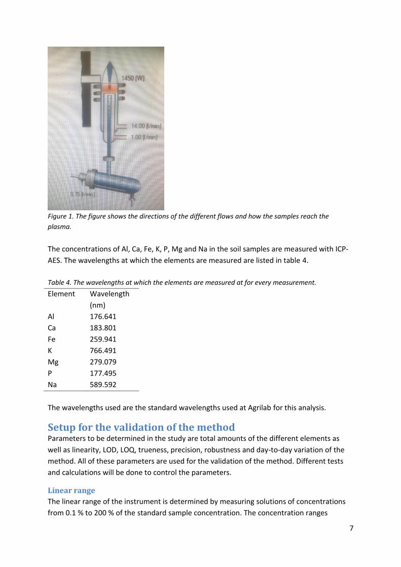
These settings are the standard for the ICP and are not optimized for the samples measured.
Figure 1 is a picture taken on the ICP showing the different flows described in table 3.
7
Figure 1. The figure shows the directions of the different flows and how the samples reach the
plasma.
The concentrations of Al, Ca, Fe, K, P, Mg and Na in the soil samples are measured with ICP-
AES. The wavelengths at which the elements are measured are listed in table 4.
Table 4. The wavelengths at which the elements are measured at for every measurement.
Element Wavelength
(nm)
Al 176.641
Ca 183.801
Fe 259.941
K 766.491
Mg 279.079
P 177.495
Na 589.592
The wavelengths used are the standard wavelengths used at Agrilab for this analysis.
Setup for the validation of the method Parameters to be determined in the study are total amounts of the different elements as
well as linearity, LOD, LOQ, trueness, precision, robustness and day-to-day variation of the
method. All of these parameters are used for the validation of the method. Different tests
and calculations will be done to control the parameters.
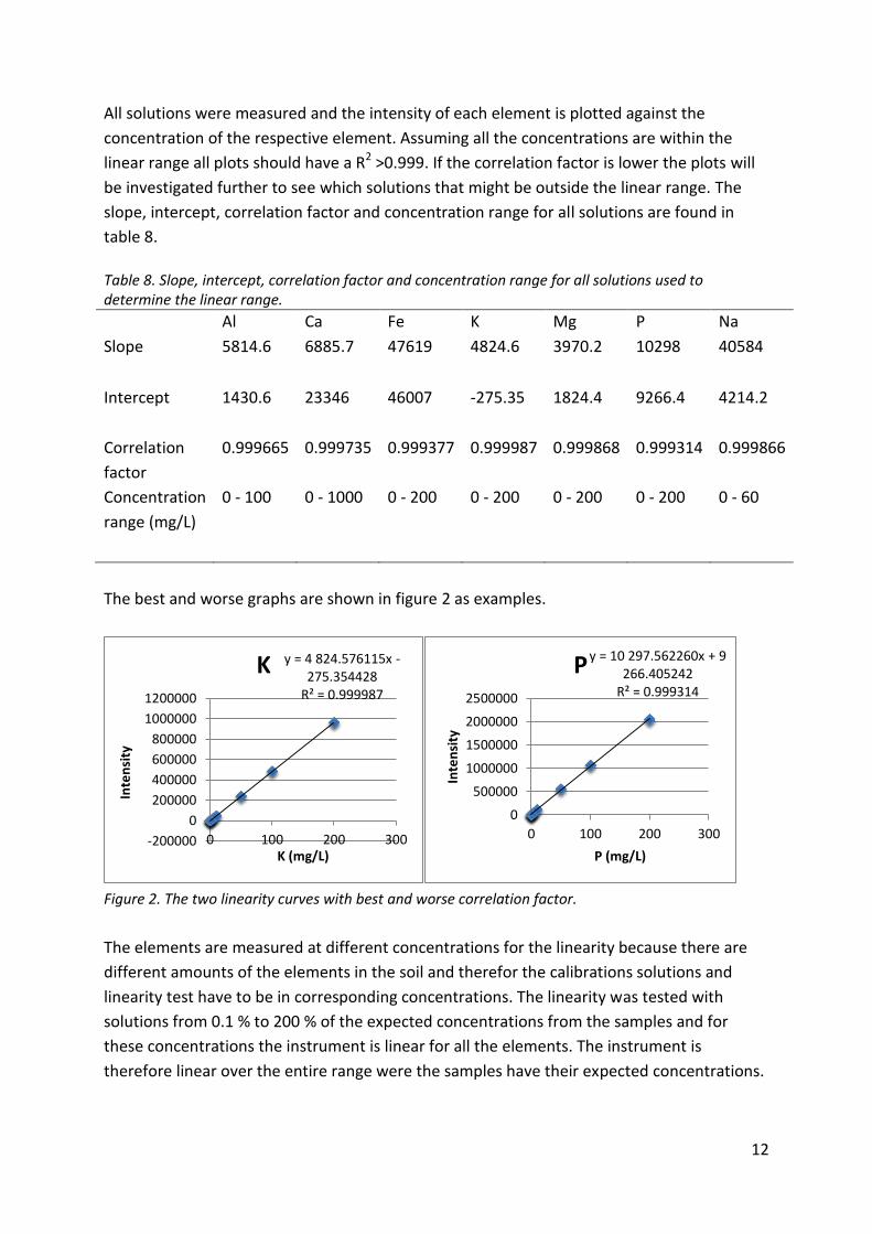
Linear range
The linear range of the instrument is determined by measuring solutions of concentrations
from 0.1 % to 200 % of the standard sample concentration. The concentration ranges
8
corresponds to concentrations between 0.05 mg/L to 200 mg/L for Al, Fe, Mg, P and K,
between 0.5 mg/L to 1000mg/L for Ca and between 0.03 and 60 mg/L for Na. The linearity is
the range in which the signal to concentration is linear. The linear range is controlled to
confirm that no samples have a concentration above of the linear range. Concentration
measured above of the linear range will be lower due to saturation of analyte outside of the
linear range. Linearity is accepted if the correlation factor R2>0.999 for the curve. For the
trueness where the samples are spiked with extra metals there is very important to know
that the samples still are within the linear range with the extra metals added, therefore the
linear range must be tested beyond the sample concentrations.
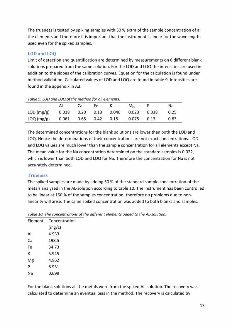
LOD and LOQ
The limit of detection of the method is determined by 2 measurements on 6 blank solutions.
From the measurements of the blanks the standard deviation is calculated. LOD of the
method is calculated by 3 ∗𝑠
𝑠𝑙𝑜𝑝𝑒 and LOQ of the method is calculated in a similar way,
10 ∗𝑠
𝑠𝑙𝑜𝑝𝑒 . Where s is the standard deviation for the intensity of the blank and the slope is
the slope for the calibrations curve.
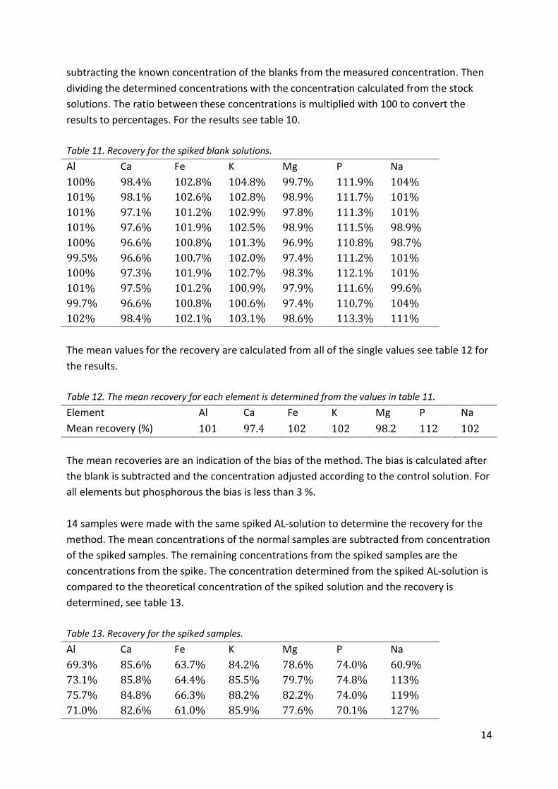
Trueness
Systematic errors lead to a bias in the method, which affect the trueness of the method, as
trueness is the lack of a bias for a method. To determine the trueness of the method,
samples and blanks are spiked with a known amount of analyte and thereafter the recovery
of the added spike is calculated and will be used to determine the trueness of the method.
The recovery is calculated by dividing the concentration calculated from the signal from the
spike with the known amount of added spike. The trueness is measured on 14 samples and
10 blanks.
One other way to determine the trueness of is to use a certified reference material (CRM)
with a known concentration and use the same sample procedure as for the normal samples.
The problem is that the method is not designed to measure total concentration, which is the
concentration that is given for the CRM samples. Thus the measured value will be lower than
the reference value and no useful information would be gained. Therefore only spiked
samples will be used to determine the trueness of the method.
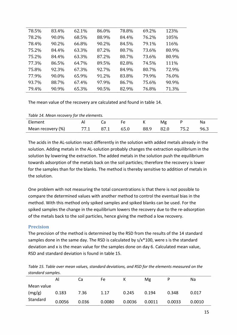
Precision
Precision is defined as the random errors of a method. [8] With low random errors the
repeatability of the method will be good. The repeatability is determined by the relative
standard deviation. RSD will be calculated from the standard deviations of samples made on
the same day. RSD is calculated by 100*s/x, where s is the standard deviation and x is the
mean value. The reason the RSD in calculated from samples made on the same day is
because day-to-day variation should not be included in the determination of RSD. A low
value of RSD indicates that the difference between the samples measured on the same day
9
is low. With a low difference between the samples made on the same day, the preparation
and analysis is precise.
RSD was also calculated on samples analysed on different days. One sample for each day for
the 5 days was used for the calculation. The value of the RSD for different days will give an
indication of the reproducibility of the method.
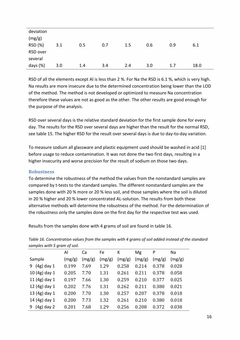
Robustness
The robustness of the method is a parameter that determines how sensitive the method it is
to small changes. If the method is very sensitive it is more difficult to get repeatability of the
results. It will be tested in two different ways, the first by adding 20% more and 20% less soil
in the samples. The second test for the method is to dilute the stock AL-solution 20% more
and 20% less to get two different concentrations of the AL-solution.
Six samples with the different preparation methods were made on two different days for a
total of 12 unique samples. The results from those samples are compared to the results of
the standard method.
To determine whether there is a difference between these results and the results from the
normal samples a two-sided t-test will be used for the results from the samples with the
special preparation methods against the normal samples. [8] If the value is lower than the
critical value for the test there is no difference, however if the value is larger than the critical
value, there is a proven difference between the results. A significant difference purposes
that the method is sensitive for changes in the preparation of the samples.
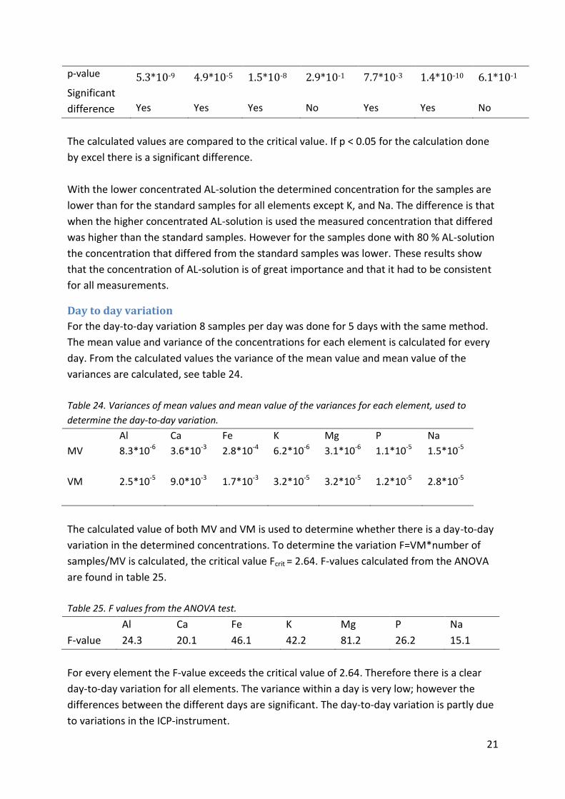
Day to day variation
Eight samples will be made and measured every day for five days and the eventual day-to-
day variation of those samples will be tested by a one-way ANOVA. [8] The ANOVA is a
comparison of the variances and mean values for sample done on different days.
Results and discussion A total of 46 standard samples were done and analysed in addition to samples with
alternative preparation methods see robustness. The standard deviation, relative standard
deviation and day-to-day variation were calculated with the standard samples. All
concentrations are mean values of two measurements for both standard samples and
robustness samples.
The concentrations of the samples are calculated by the concentrations given from the
measurements. The ICP program give the concentrations in mg/L, by multiplying the value
with the volume and dividing it by the added amount of soil the units is converted to mg/g.
Before and after the samples are measured a control solution with concentration, see table
10
5, is measured. The quotient for the known control solutions concentration and the
measured concentration is used to adjust the calculated values of the samples for the bias in
the measured concentration.
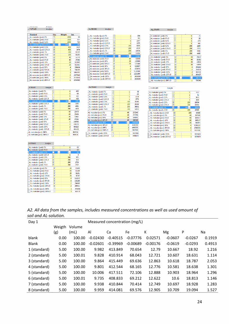
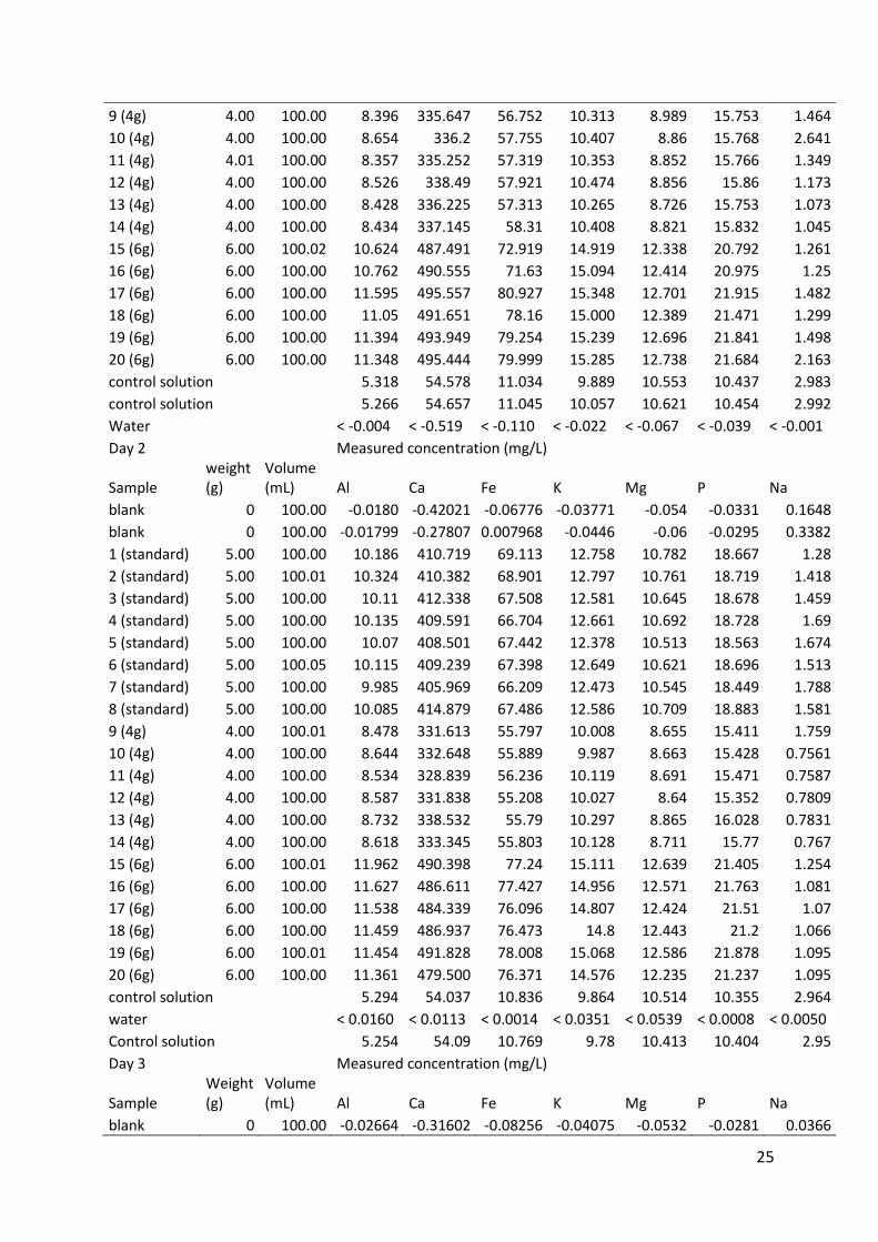
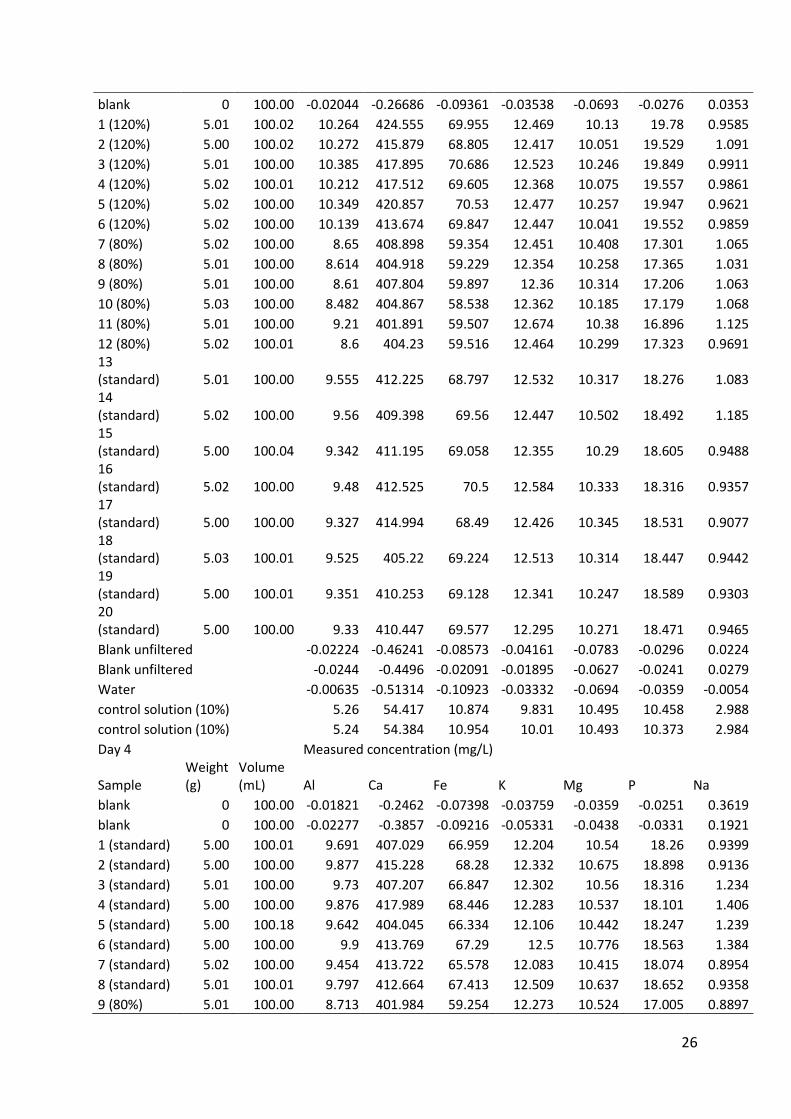
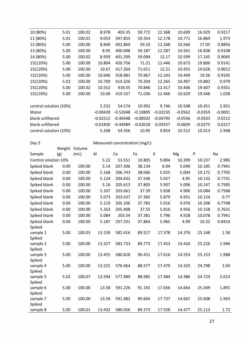
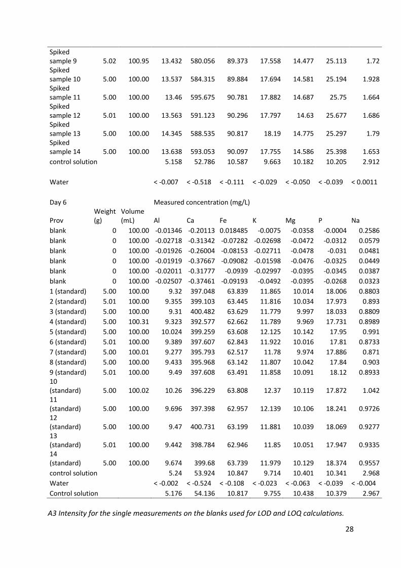
Data from all the measurements are found in the appendix.
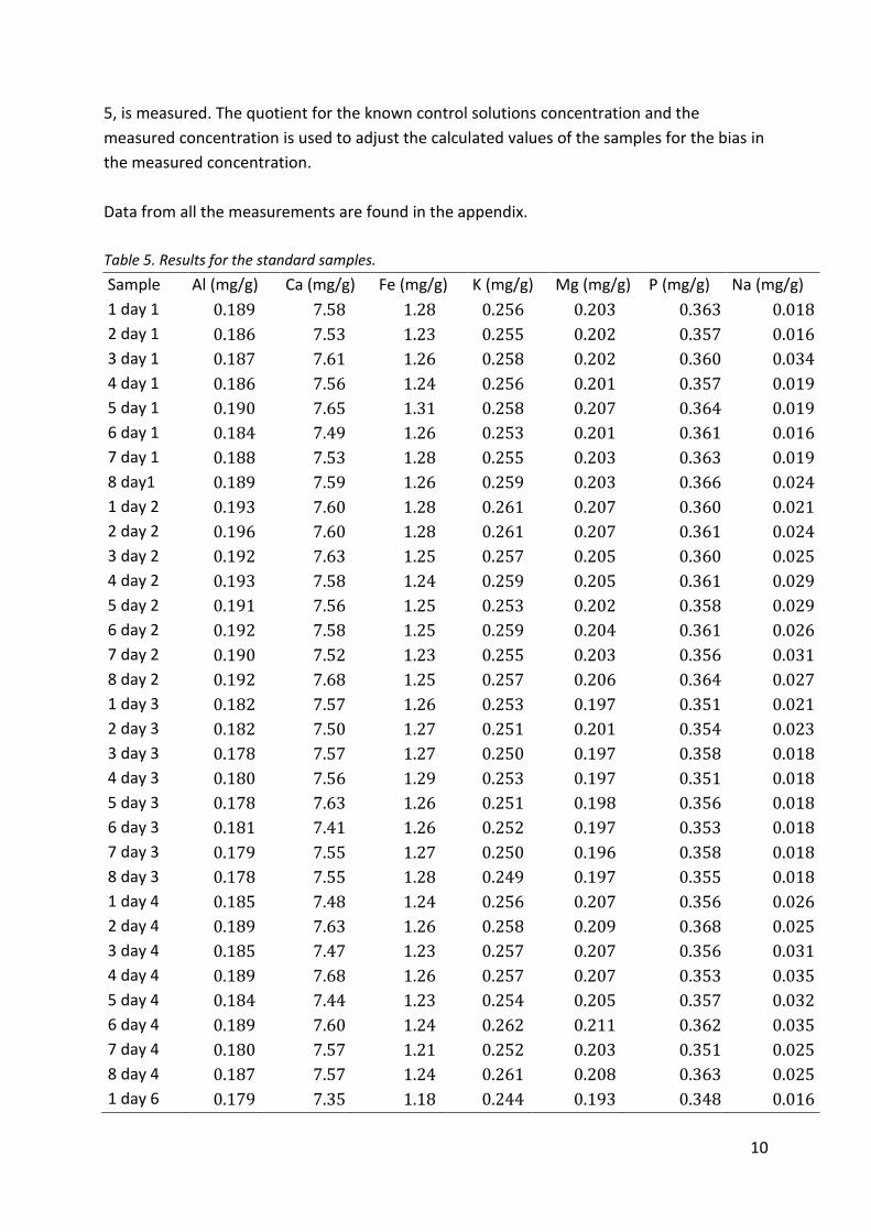
Table 5. Results for the standard samples.
Sample Al (mg/g) Ca (mg/g) Fe (mg/g) K (mg/g) Mg (mg/g) P (mg/g) Na (mg/g)
1 day 1 0.189 7.58 1.28 0.256 0.203 0.363 0.018
2 day 1 0.186 7.53 1.23 0.255 0.202 0.357 0.016
3 day 1 0.187 7.61 1.26 0.258 0.202 0.360 0.034
4 day 1 0.186 7.56 1.24 0.256 0.201 0.357 0.019
5 day 1 0.190 7.65 1.31 0.258 0.207 0.364 0.019
6 day 1 0.184 7.49 1.26 0.253 0.201 0.361 0.016
7 day 1 0.188 7.53 1.28 0.255 0.203 0.363 0.019
8 day1 0.189 7.59 1.26 0.259 0.203 0.366 0.024
1 day 2 0.193 7.60 1.28 0.261 0.207 0.360 0.021
2 day 2 0.196 7.60 1.28 0.261 0.207 0.361 0.024
3 day 2 0.192 7.63 1.25 0.257 0.205 0.360 0.025
4 day 2 0.193 7.58 1.24 0.259 0.205 0.361 0.029
5 day 2 0.191 7.56 1.25 0.253 0.202 0.358 0.029
6 day 2 0.192 7.58 1.25 0.259 0.204 0.361 0.026
7 day 2 0.190 7.52 1.23 0.255 0.203 0.356 0.031
8 day 2 0.192 7.68 1.25 0.257 0.206 0.364 0.027
1 day 3 0.182 7.57 1.26 0.253 0.197 0.351 0.021
2 day 3 0.182 7.50 1.27 0.251 0.201 0.354 0.023
3 day 3 0.178 7.57 1.27 0.250 0.197 0.358 0.018
4 day 3 0.180 7.56 1.29 0.253 0.197 0.351 0.018
5 day 3 0.178 7.63 1.26 0.251 0.198 0.356 0.018
6 day 3 0.181 7.41 1.26 0.252 0.197 0.353 0.018
7 day 3 0.179 7.55 1.27 0.250 0.196 0.358 0.018
8 day 3 0.178 7.55 1.28 0.249 0.197 0.355 0.018
1 day 4 0.185 7.48 1.24 0.256 0.207 0.356 0.026
2 day 4 0.189 7.63 1.26 0.258 0.209 0.368 0.025
3 day 4 0.185 7.47 1.23 0.257 0.207 0.356 0.031
4 day 4 0.189 7.68 1.26 0.257 0.207 0.353 0.035
5 day 4 0.184 7.44 1.23 0.254 0.205 0.357 0.032
6 day 4 0.189 7.60 1.24 0.262 0.211 0.362 0.035
7 day 4 0.180 7.57 1.21 0.252 0.203 0.351 0.025
8 day 4 0.187 7.57 1.24 0.261 0.208 0.363 0.025
1 day 6 0.179 7.35 1.18 0.244 0.193 0.348 0.016
11
2 day 6 0.180 7.38 1.17 0.243 0.193 0.347 0.016
3 day 6 0.179 7.42 1.18 0.243 0.193 0.349 0.016
4 day 6 0.180 7.29 1.16 0.243 0.193 0.344 0.017
5 day 6 0.193 7.40 1.18 0.250 0.195 0.347 0.018
6 day 6 0.180 7.35 1.16 0.245 0.193 0.344 0.016
7 day 6 0.179 7.33 1.16 0.243 0.192 0.346 0.016
8 day 6 0.182 7.33 1.17 0.243 0.194 0.345 0.017
9 day 6 0.182 7.35 1.17 0.244 0.194 0.350 0.016
10 day 6 0.197 7.34 1.18 0.255 0.195 0.346 0.019
11 day 6 0.187 7.36 1.16 0.250 0.195 0.353 0.018
12 day 6 0.182 7.42 1.17 0.245 0.194 0.349 0.017
13 day 6 0.181 7.37 1.16 0.244 0.193 0.346 0.017
14 day 6 0.186 7.40 1.18 0.247 0.195 0.355 0.018
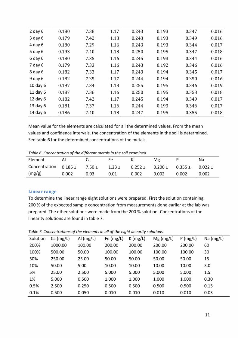
Mean value for the elements are calculated for all the determined values. From the mean
values and confidence intervals, the concentration of the elements in the soil is determined.
See table 6 for the determined concentrations of the metals.
Table 6. Concentration of the different metals in the soil examined.
Element Al Ca Fe K Mg P Na
Concentration
(mg/g)
0.185 ±
0.002
7.50 ±
0.03
1.23 ±
0.01
0.252 ±
0.002
0.200 ±
0.002
0.355 ±
0.002
0.022 ±
0.002
Linear range
To determine the linear range eight solutions were prepared. First the solution containing
200 % of the expected sample concentration from measurements done earlier at the lab was
prepared. The other solutions were made from the 200 % solution. Concentrations of the
linearity solutions are found in table 7.
Table 7. Concentrations of the elements in all of the eight linearity solutions.
Solution Ca (mg/L) Al (mg/L) Fe (mg/L) K (mg/L) Mg (mg/L) P (mg/L) Na (mg/L)
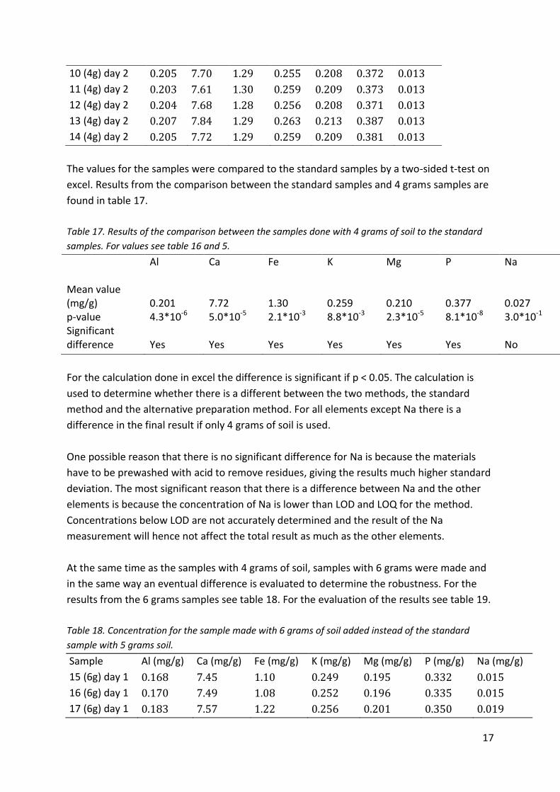
The values for the samples were compared to the standard samples by a two-sided t-test on
excel. Results from the comparison between the standard samples and 4 grams samples are
found in table 17.
Table 17. Results of the comparison between the samples done with 4 grams of soil to the standard
samples. For values see table 16 and 5.
Al Ca Fe K Mg P Na Mean value (mg/g) 0.201 7.72 1.30 0.259 0.210 0.377 0.027 p-value 4.3*10-6 5.0*10-5 2.1*10-3 8.8*10-3 2.3*10-5 8.1*10-8 3.0*10-1 Significant difference
Yes
Yes
Yes
Yes
Yes
Yes
No
For the calculation done in excel the difference is significant if p < 0.05. The calculation is
used to determine whether there is a different between the two methods, the standard
method and the alternative preparation method. For all elements except Na there is a
difference in the final result if only 4 grams of soil is used.
One possible reason that there is no significant difference for Na is because the materials
have to be prewashed with acid to remove residues, giving the results much higher standard
deviation. The most significant reason that there is a difference between Na and the other
elements is because the concentration of Na is lower than LOD and LOQ for the method.
Concentrations below LOD are not accurately determined and the result of the Na
measurement will hence not affect the total result as much as the other elements.
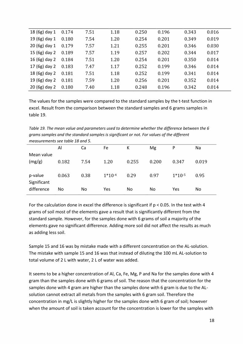
At the same time as the samples with 4 grams of soil, samples with 6 grams were made and
in the same way an eventual difference is evaluated to determine the robustness. For the
results from the 6 grams samples see table 18. For the evaluation of the results see table 19.
Table 18. Concentration for the sample made with 6 grams of soil added instead of the standard
sample with 5 grams soil.
Sample Al (mg/g) Ca (mg/g) Fe (mg/g) K (mg/g) Mg (mg/g) P (mg/g) Na (mg/g)