1 Orlando, Florida August 26, 2009 UXO/Countermine/Range Forum L-P Song a , L R Pasion b , S D Billings b and D W Oldenburg a b Sky Research, Inc, Ashland, Oregon a Geophysical Inversion Facility Univ. of British Columbia, Vancouver Canada Determining Equivalent Dipole Number by Information Theoretic Criteria
Transcript
1
Orlando, FloridaAugust 26, 2009
UXO/Countermine/Range Forum
L-P Songa, L R Pasionb, S D Billingsb
and D W Oldenburga
bSky Research, Inc, Ashland, Oregon
aGeophysical Inversion FacilityUniv. of British Columbia, Vancouver Canada
Determining Equivalent Dipole Number by Information Theoretic Criteria
2
• Motivation and Problem Formulation • Information-Theoretical Criteria • Applications: EM63, TEMTADS• Summary
Outline
3
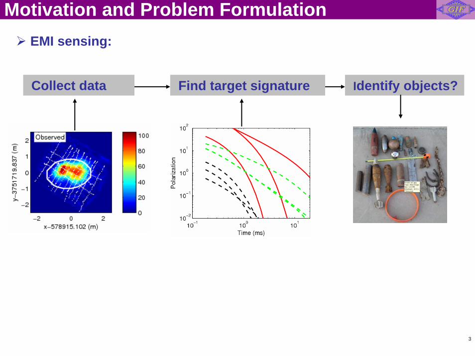
Motivation and Problem FormulationEMI sensing:
Collect data Find target signature Identify objects?
4
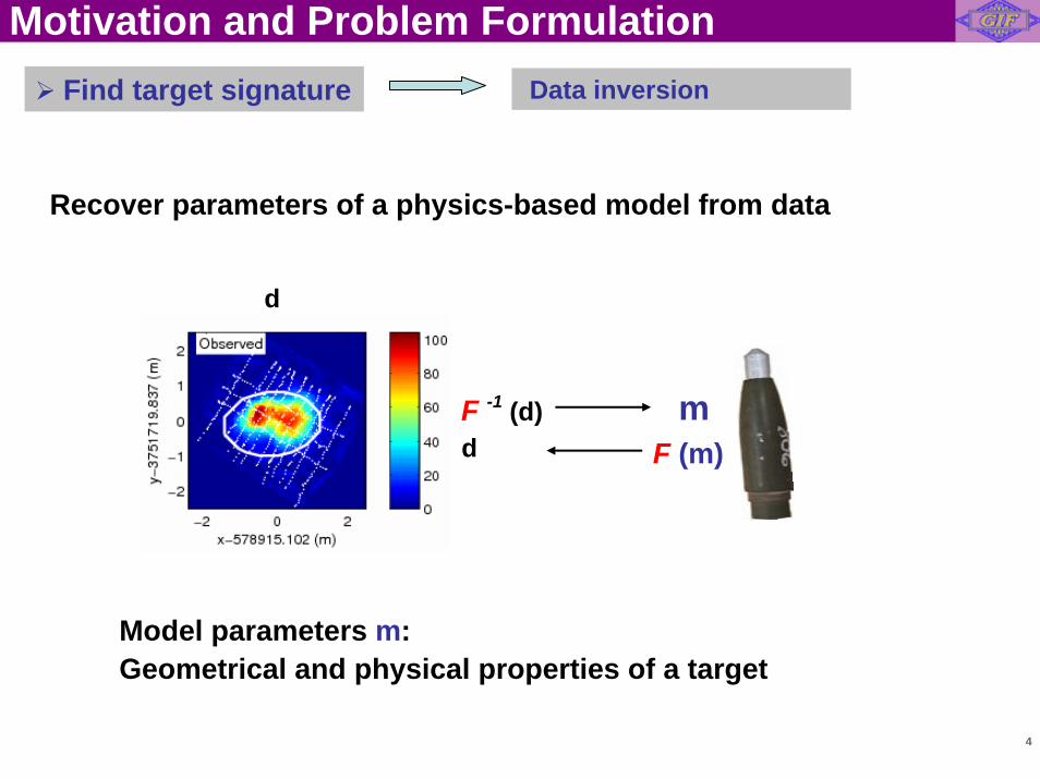
Find target signature Data inversion
Model parameters m:Geometrical and physical properties of a target
d
F -1 (d)
Recover parameters of a physics-based model from data
md F (m)
Motivation and Problem Formulation
5
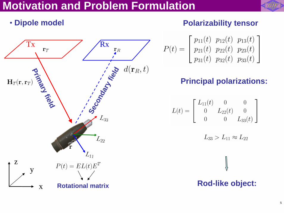
• Dipole model Polarizability tensor
y
x
z
Tx Rx
Primary field
Seco
ndar
y fie
ld
Principal polarizations:
Rod-like object:Rotational matrix
Motivation and Problem Formulation
6
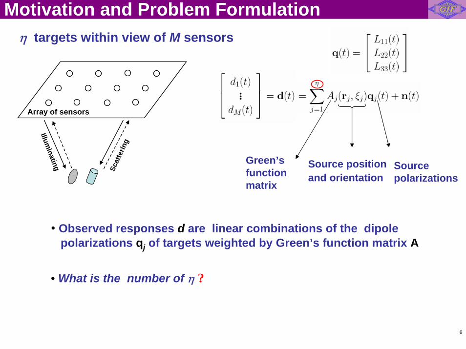
η targets within view of M sensors
Green’s function matrix
Source positionand orientation
Source polarizations
• Observed responses d are linear combinations of the dipole polarizations qj of targets weighted by Green’s function matrix A
Scat
terin
g
Illuminating
Array of sensors
• What is the number of η ?
Motivation and Problem Formulation
7
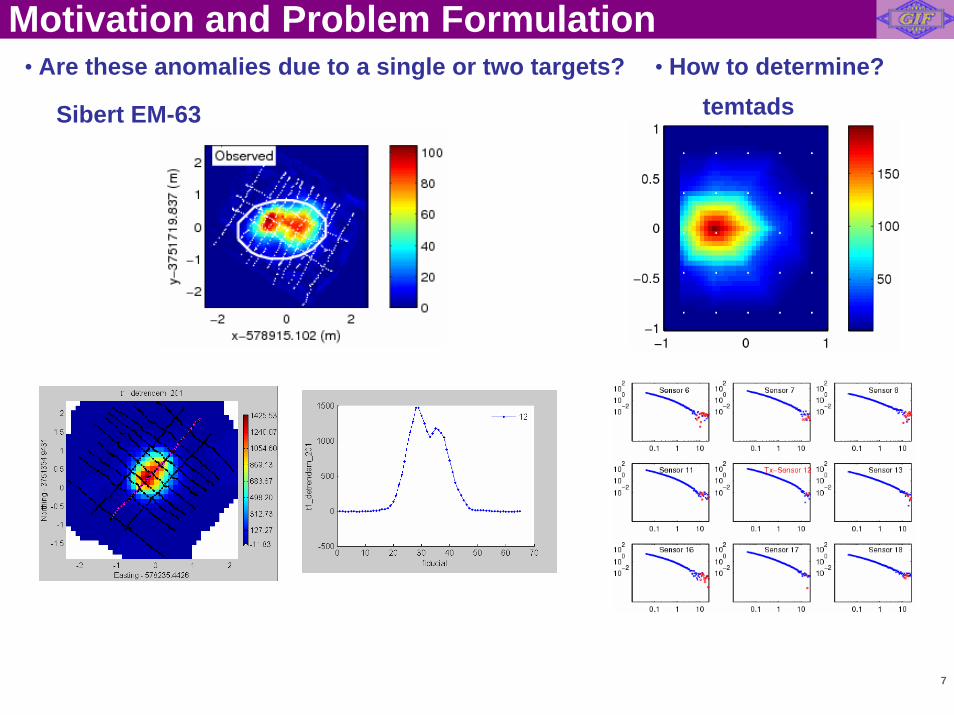
Sibert EM-63
• Are these anomalies due to a single or two targets?temtads
• How to determine?
Motivation and Problem Formulation
8
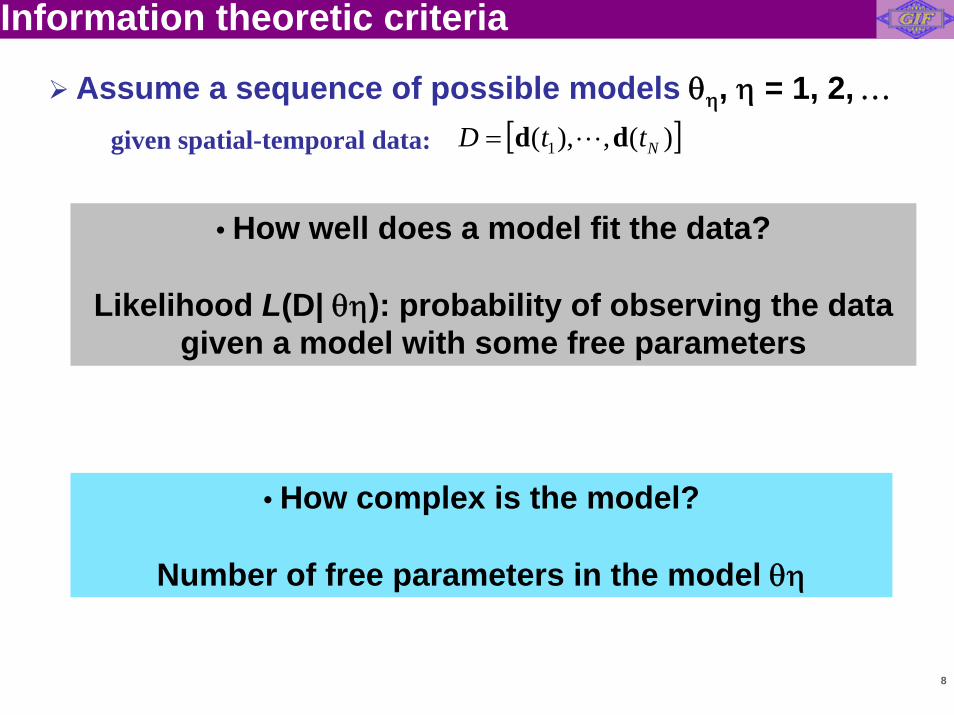
Assume a sequence of possible models θη, η = 1, 2, …
Information theoretic criteria
• How well does a model fit the data?
Likelihood L(D| θη): probability of observing the data given a model with some free parameters
• How complex is the model?
Number of free parameters in the model θη
given spatial-temporal data: [ ])(,),( 1 NttD dd L=
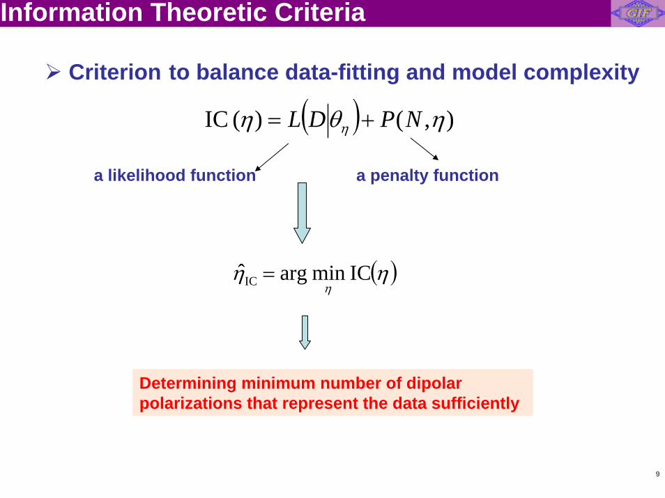
9
Information Theoretic Criteria
a likelihood function a penalty function
( ) ),()(IC ηθη η NPDL +=
Criterion to balance data-fitting and model complexity
( )ηηη
IC min arg ˆIC =
Determining minimum number of dipolar polarizations that represent the data sufficiently
10
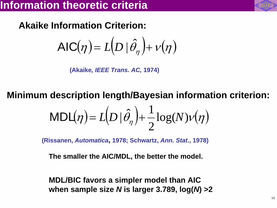
Information theoretic criteria
( ) ( ) ( )ηνθη η )log(21ˆ| NDL +=MDL
( )
MDL/BIC favors a simpler model than AIC when sample size N is larger 3.789, log(N) >2
( ) ( )ηνθη η += ˆ|DLAIC
Akaike Information Criterion:
Minimum description length/Bayesian information criterion:
The smaller the AIC/MDL, the better the model.
(Akaike, IEEE Trans. AC, 1974)
(Rissanen, Automatica, 1978; Schwartz, Ann. Stat., 1978)
11
Information theoretic criteria
What is behind the ITC?
• Principle of Parsimony (Simplicity):A complicated model (too many parameters) is not desirable: its ‘good’ performance might be misleading.
• Data-fitting performance is overseen with model complexity.
12
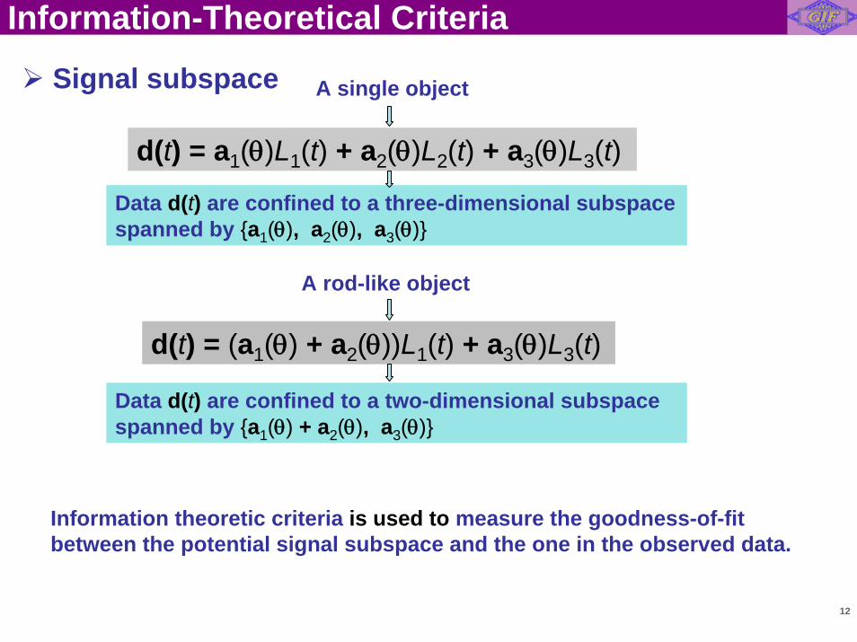
Information-Theoretical Criteria
Signal subspace
Data d(t) are confined to a three-dimensional subspace spanned by {a1(θ), a2(θ), a3(θ)}
Information theoretic criteria is used to measure the goodness-of-fit between the potential signal subspace and the one in the observed data.
d(t) = a1(θ)L1(t) + a2(θ)L2(t) + a3(θ)L3(t)
A single object
Data d(t) are confined to a two-dimensional subspace spanned by {a1(θ) + a2(θ), a3(θ)}
d(t) = (a1(θ) + a2(θ))L1(t) + a3(θ)L3(t)
A rod-like object
13
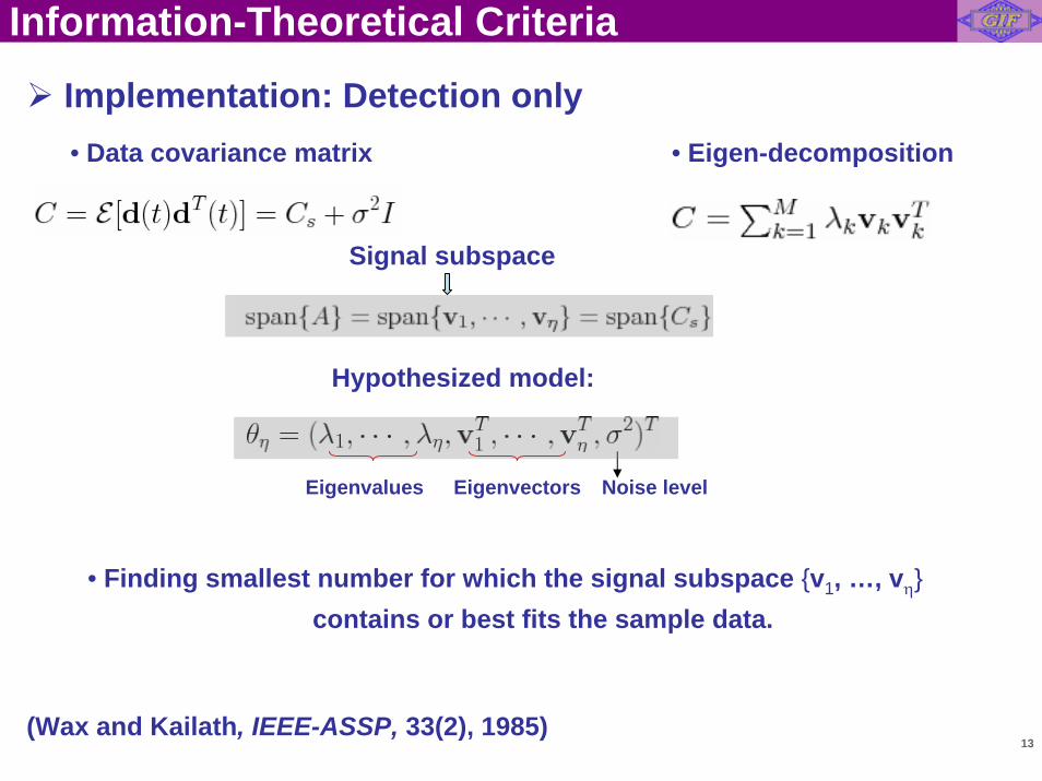
Information-Theoretical Criteria
• Data covariance matrix
EigenvectorsEigenvalues
Implementation: Detection only
Signal subspace
• Eigen-decomposition
Hypothesized model:
(Wax and Kailath, IEEE-ASSP, 33(2), 1985)
• Finding smallest number for which the signal subspace {v1, …, vη}contains or best fits the sample data.
Noise level
14
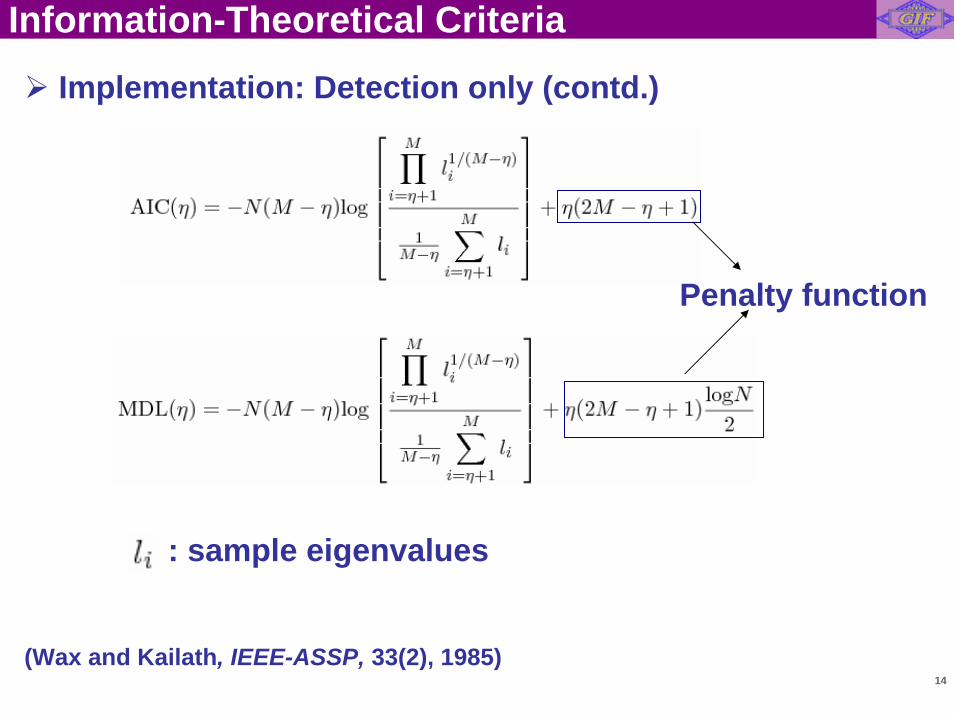
Information-Theoretical Criteria
Implementation: Detection only (contd.)
(Wax and Kailath, IEEE-ASSP, 33(2), 1985)
Penalty function
: sample eigenvalues
15
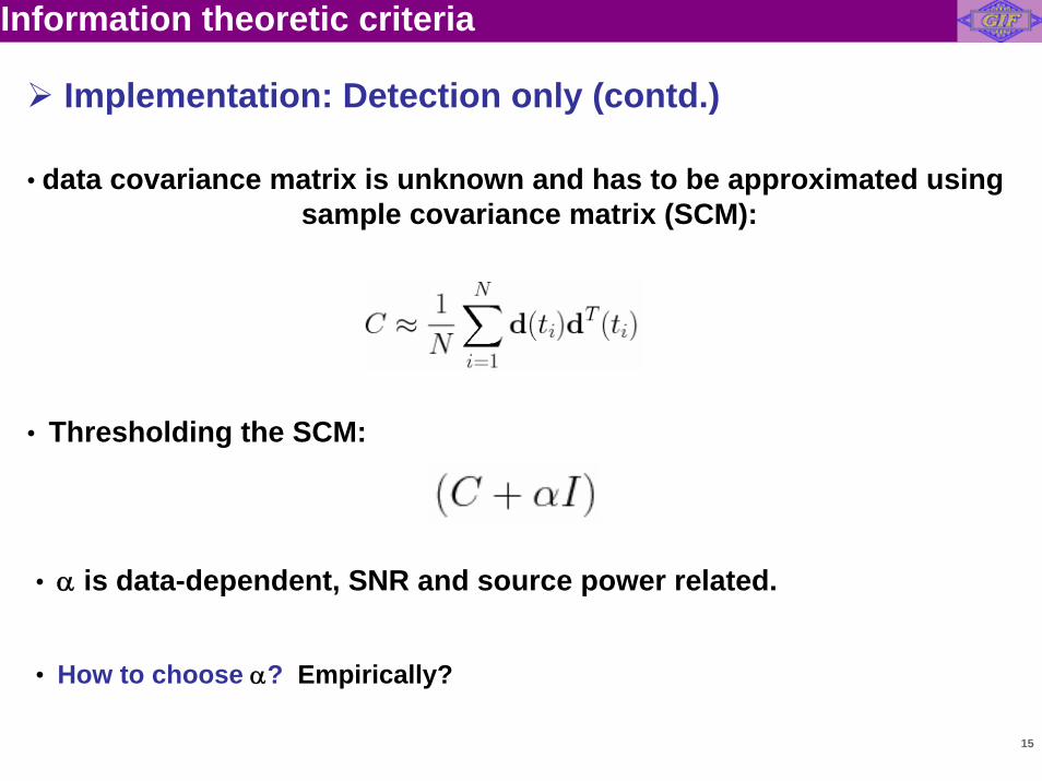
• data covariance matrix is unknown and has to be approximated using sample covariance matrix (SCM):
Information theoretic criteria
Implementation: Detection only (contd.)
• Thresholding the SCM:
• How to choose α? Empirically?
• α is data-dependent, SNR and source power related.
16
Information theoretic criteria
• The eigen-structure-based criteria can be sub-optimal or even fail due to uncertainty in SCM.
• It may be desirable to determine the number of sources and estimate their locations jointly.
• Consider that the measured data is a function of both the number of source polarizations and their locations.
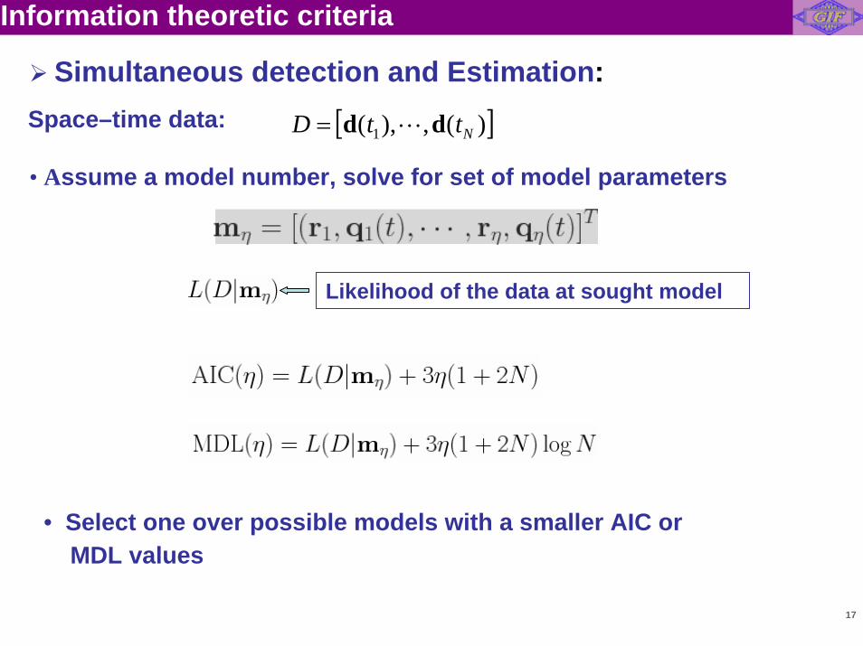
17
Space–time data: [ ])(,),( 1 NttD dd L=
• Assume a model number, solve for set of model parameters
Likelihood of the data at sought model
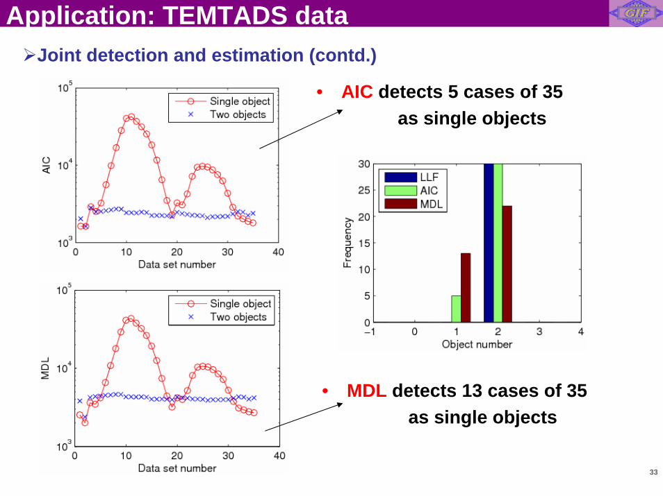
• Select one over possible models with a smaller AIC or MDL values
Simultaneous detection and Estimation:
Information theoretic criteria
18
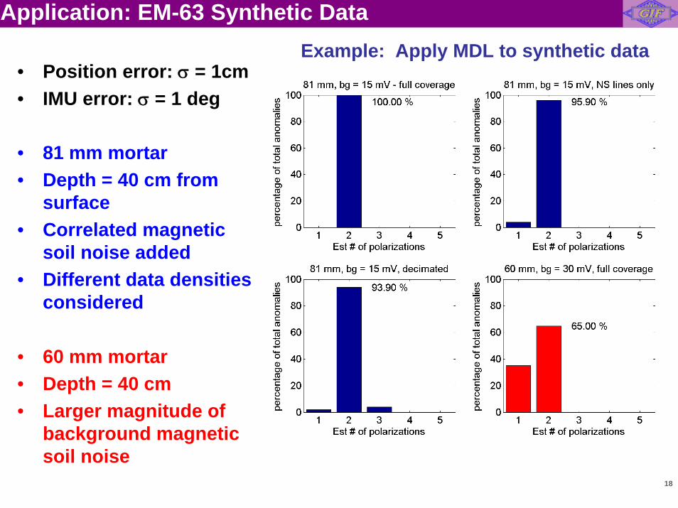
Application: EM-63 Synthetic Data
• Position error: σ = 1cm• IMU error: σ = 1 deg
• 81 mm mortar• Depth = 40 cm from
surface• Correlated magnetic
soil noise added• Different data densities
considered
• 60 mm mortar• Depth = 40 cm• Larger magnitude of
background magnetic soil noise
Example: Apply MDL to synthetic data
19
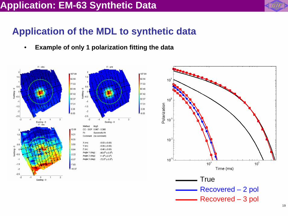
Application: EM-63 Synthetic Data
Application of the MDL to synthetic data
TrueRecovered – 2 polRecovered – 3 pol
• Example of only 1 polarization fitting the data
20
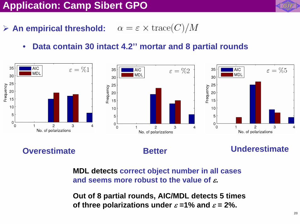
Application: Camp Sibert GPO
An empirical threshold:
• Data contain 30 intact 4.2’’ mortar and 8 partial rounds
Overestimate Better Underestimate
MDL detects correct object number in all cases and seems more robust to the value of ε.
Out of 8 partial rounds, AIC/MDL detects 5 times of three polarizations under ε =1% and ε = 2%.
21
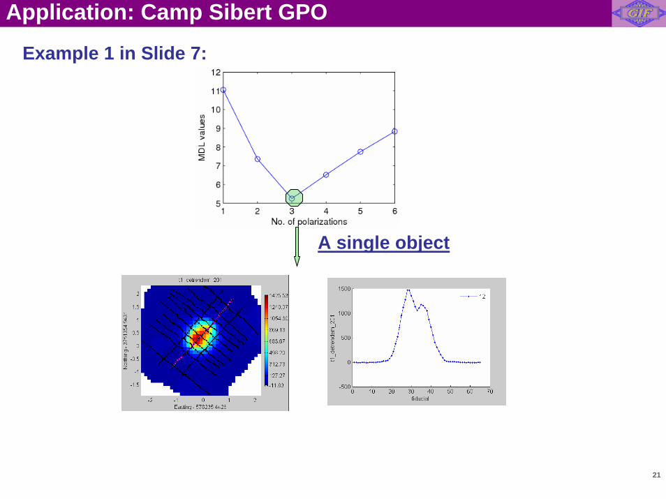
Application: Camp Sibert GPO
Example 1 in Slide 7:
A single object
22
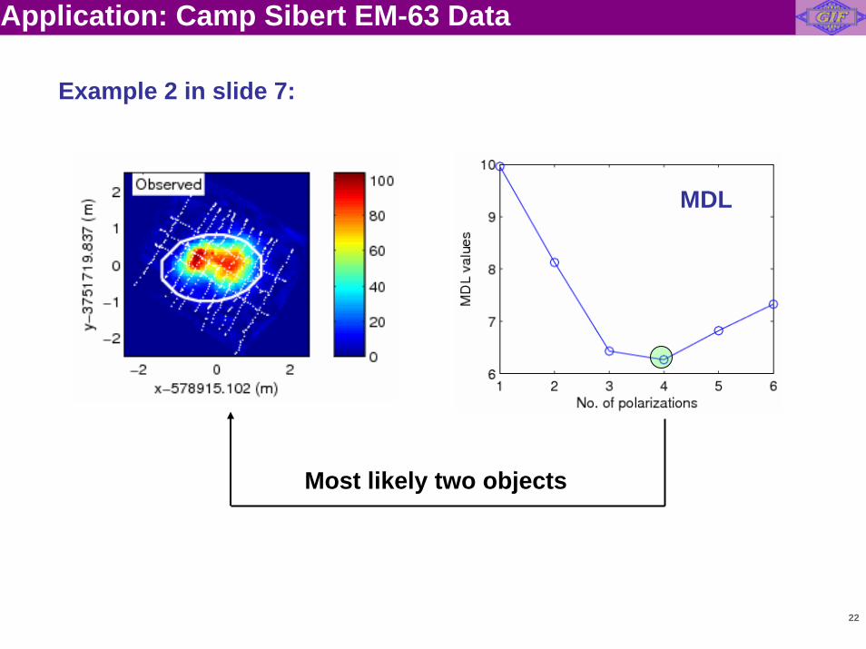
Application: Camp Sibert EM-63 Data
Example 2 in slide 7:
MDL
Most likely two objects
23
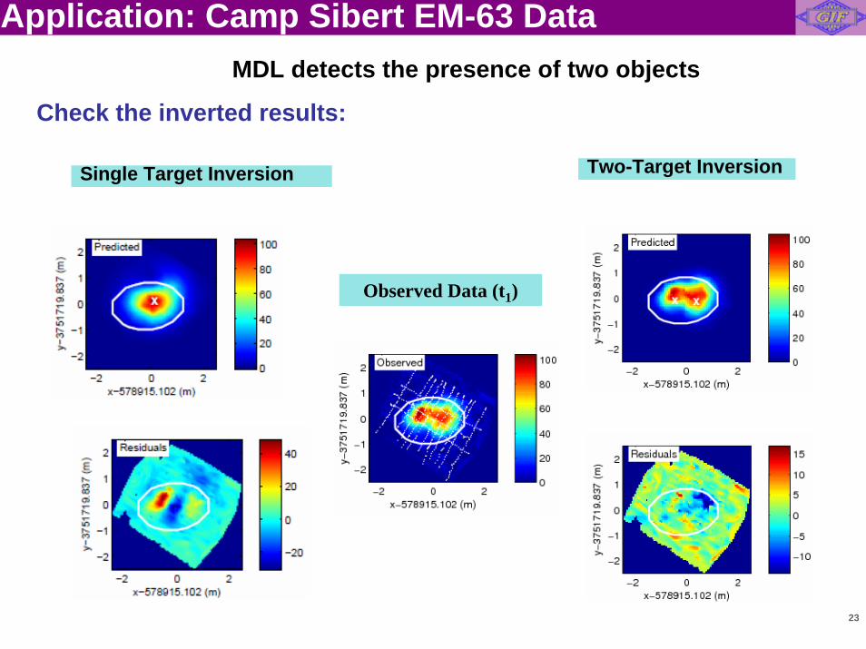
Check the inverted results:
Two-Target InversionSingle Target Inversion
Observed Data (t1)
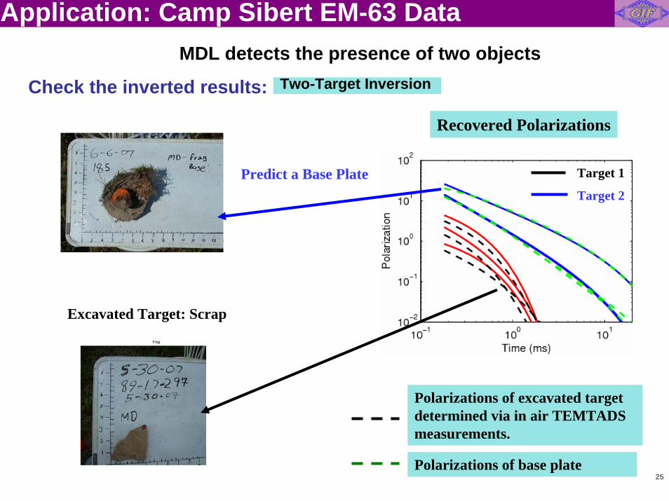
Application: Camp Sibert EM-63 DataMDL detects the presence of two objects
24
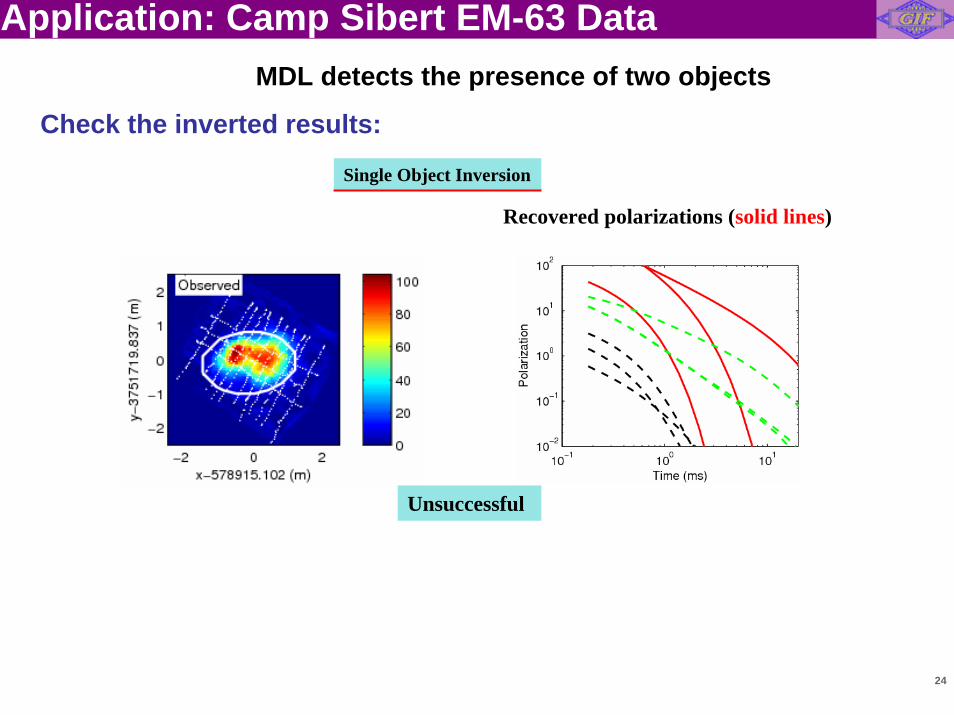
Single Object Inversion
Recovered polarizations (solid lines)
Unsuccessful
Application: Camp Sibert EM-63 Data
Check the inverted results:
MDL detects the presence of two objects
25
Recovered Polarizations
Polarizations of excavated target determined via in air TEMTADS measurements.
Polarizations of base plate
Excavated Target: Scrap
Predict a Base PlateTarget 2
Target 1
Application: Camp Sibert EM-63 Data
Check the inverted results:
MDL detects the presence of two objectsTwo-Target Inversion
26
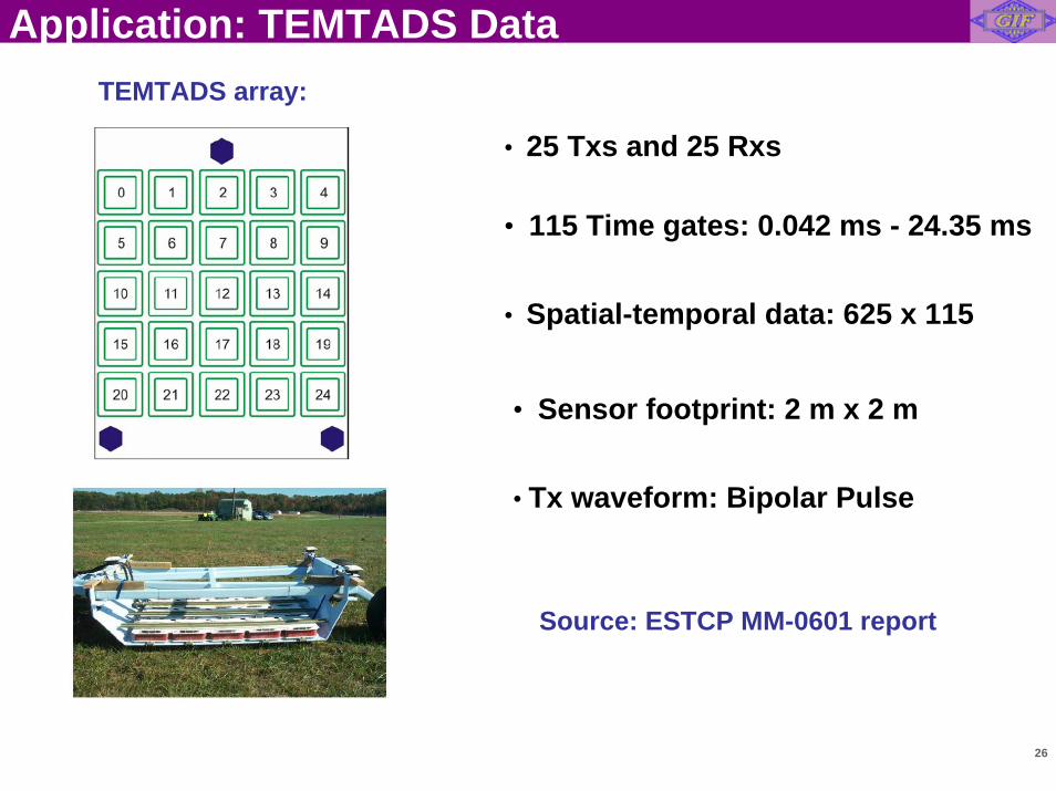
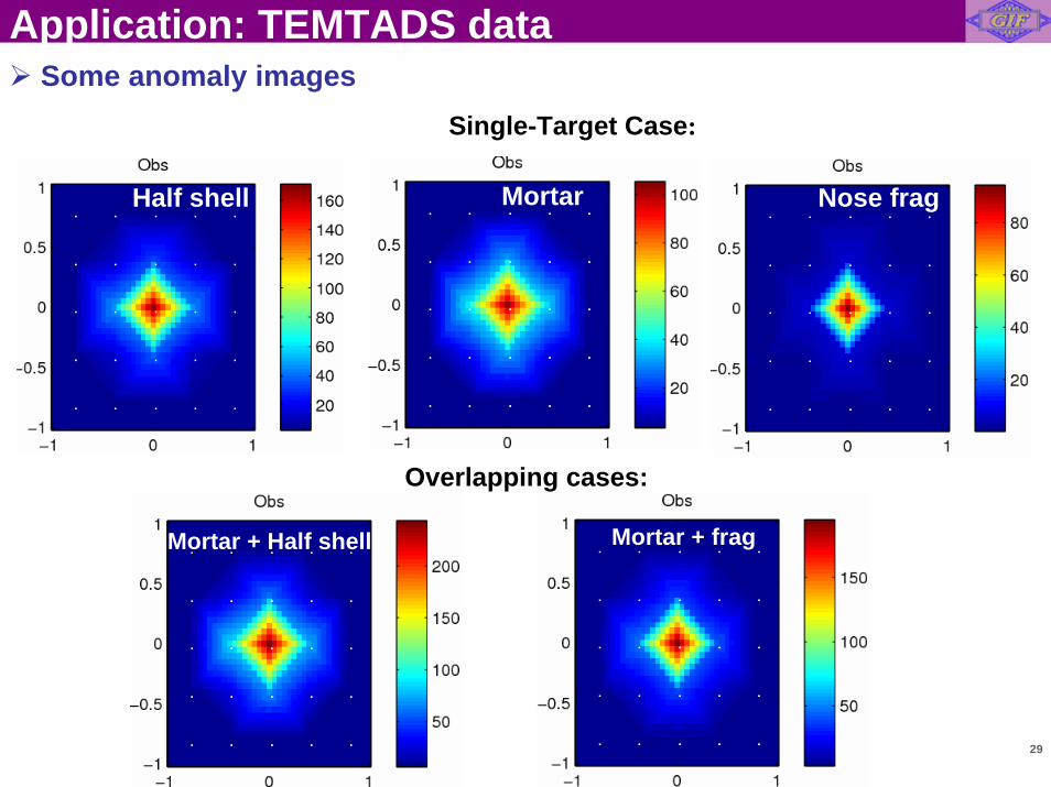
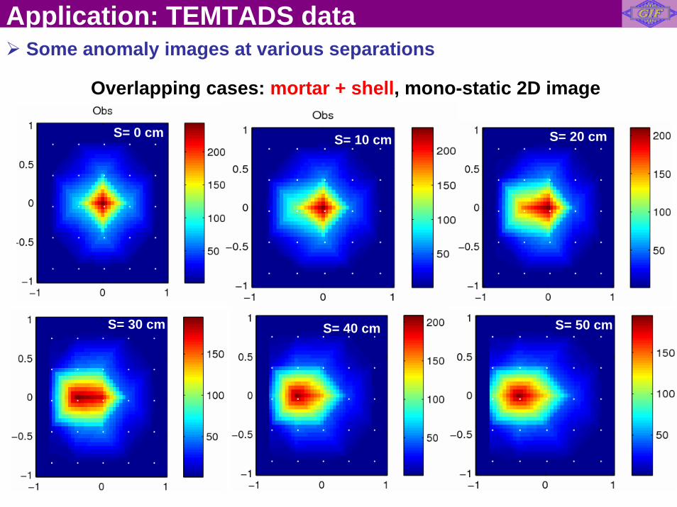
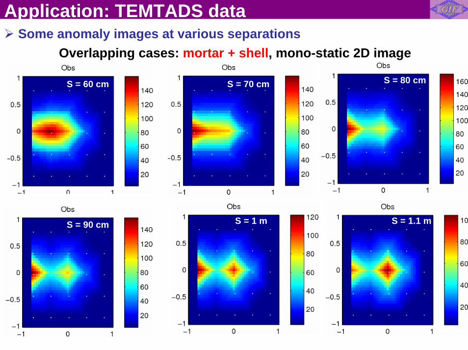
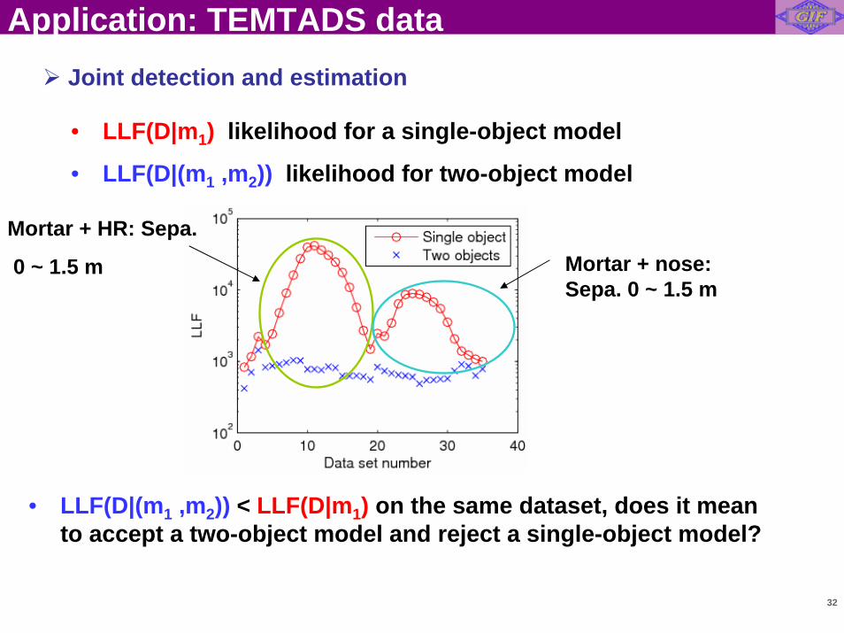
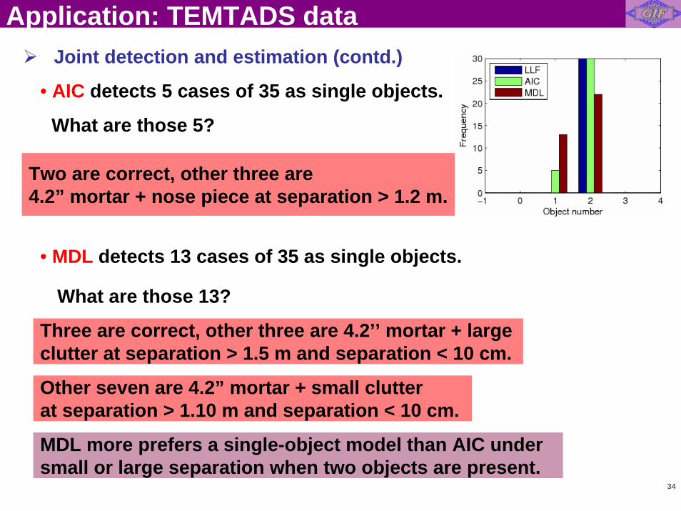
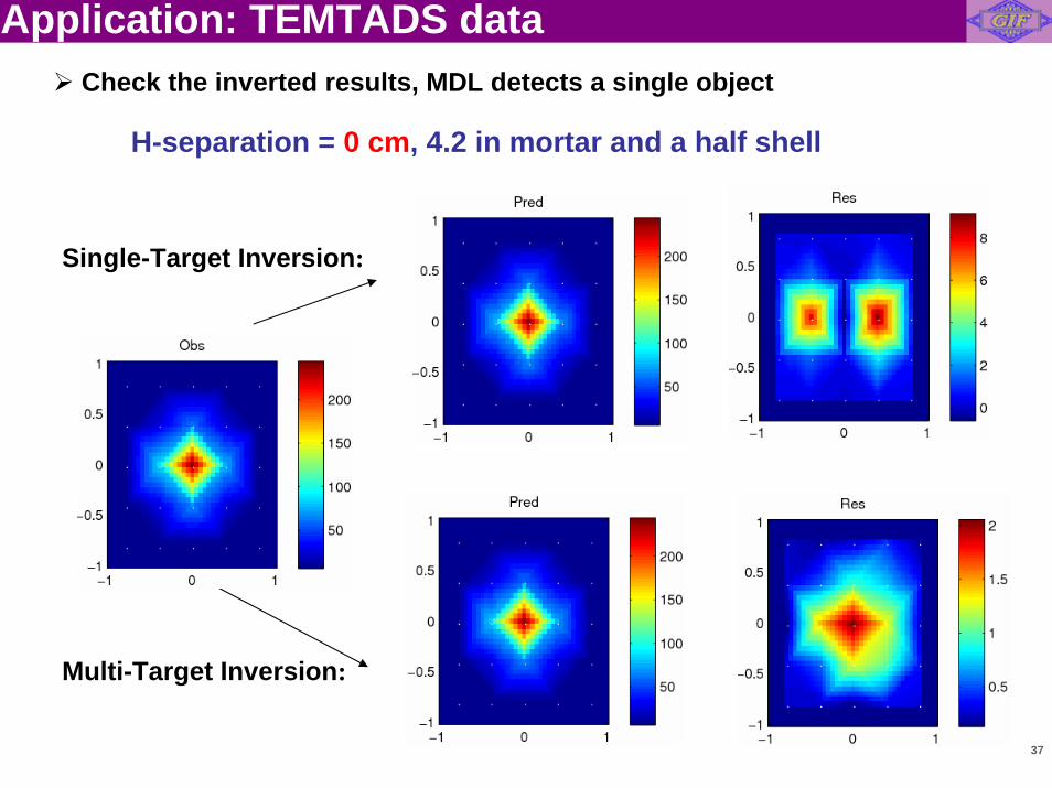
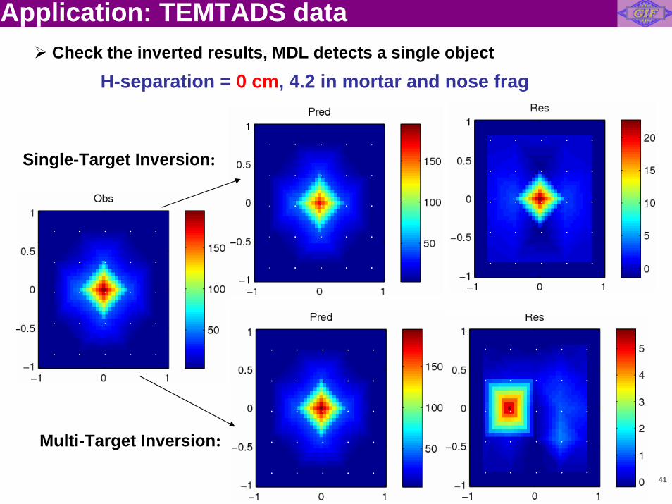
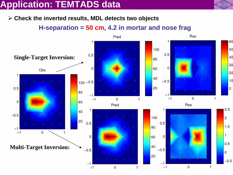
Application: TEMTADS Data
• Tx waveform: Bipolar Pulse
• 115 Time gates: 0.042 ms - 24.35 ms
• Spatial-temporal data: 625 x 115
• 25 Txs and 25 Rxs
• Sensor footprint: 2 m x 2 m
TEMTADS array:
Source: ESTCP MM-0601 report
27
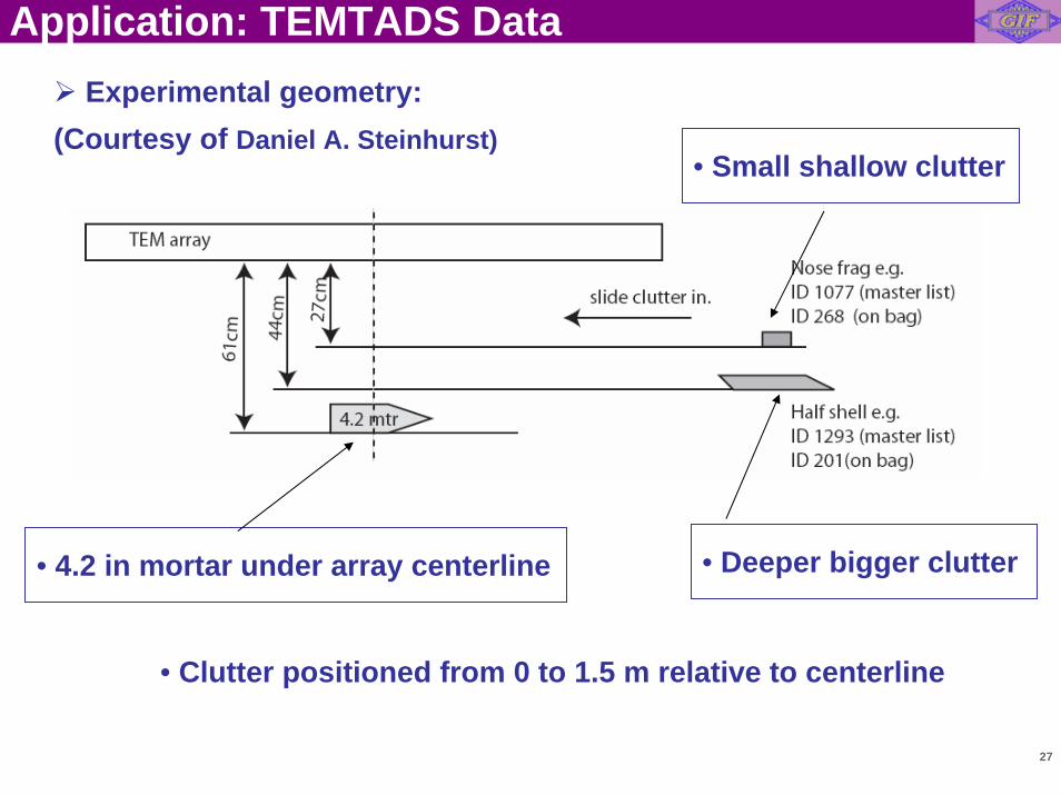
Experimental geometry:(Courtesy of Daniel A. Steinhurst)
• 4.2 in mortar under array centerline
• Small shallow clutter
• Deeper bigger clutter
• Clutter positioned from 0 to 1.5 m relative to centerline
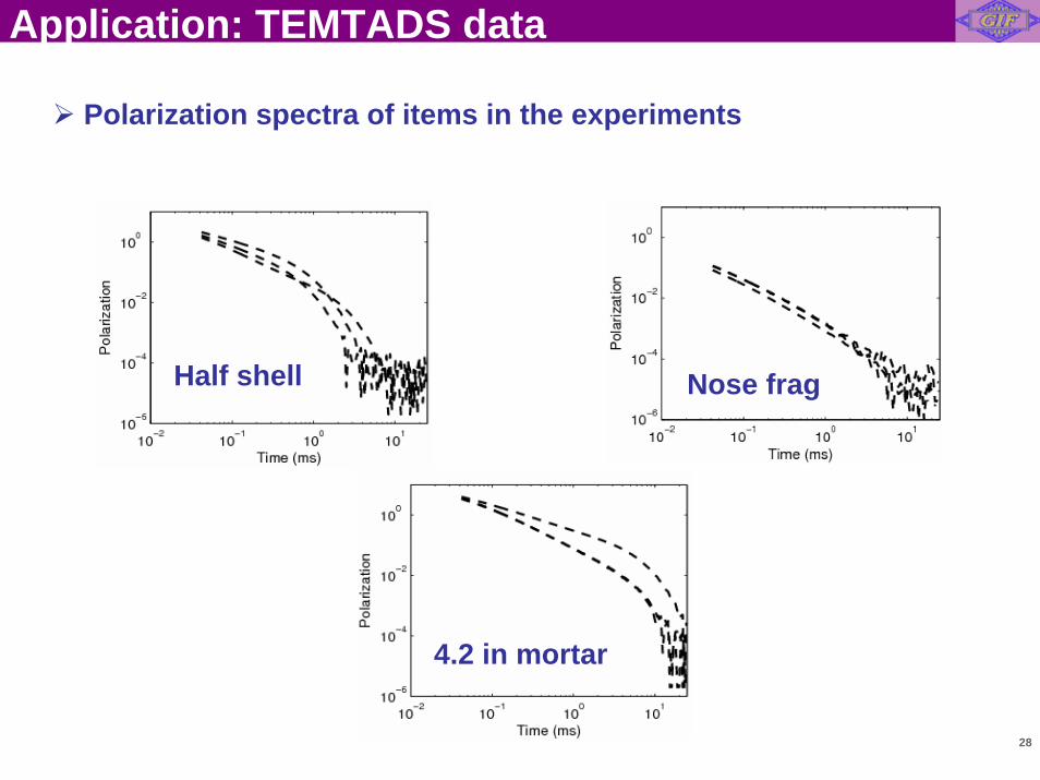
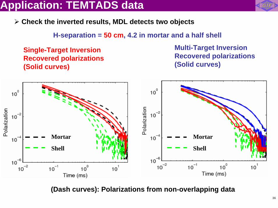
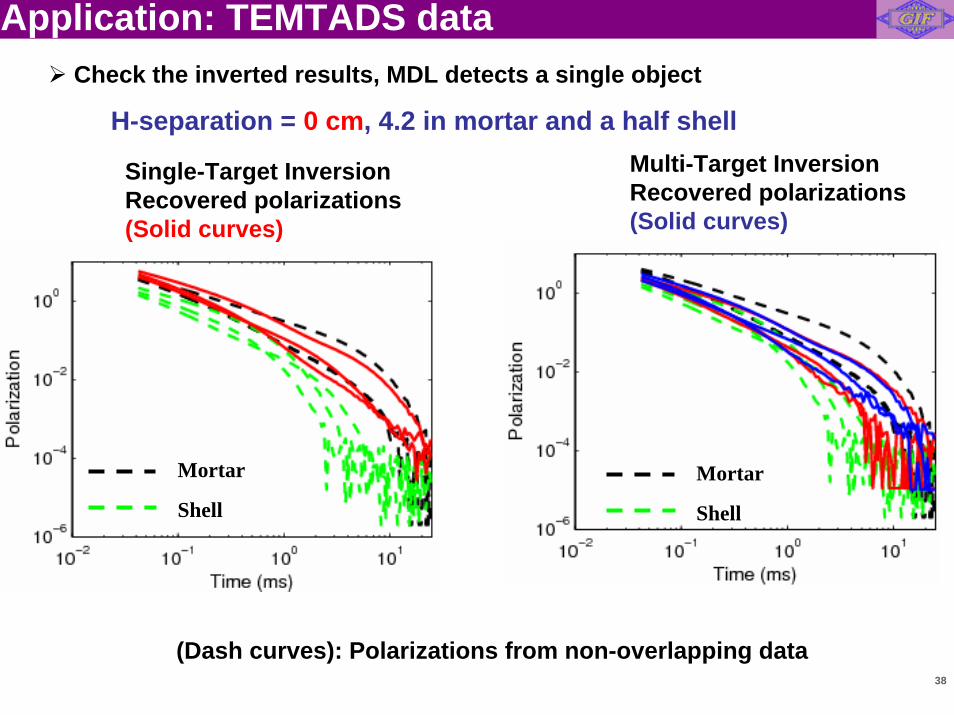
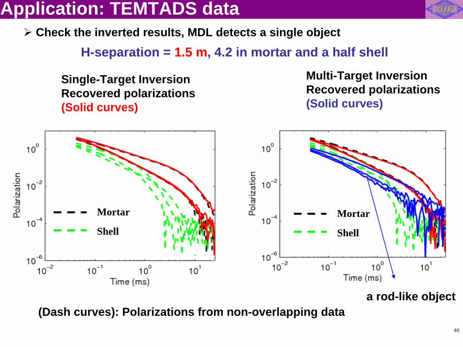
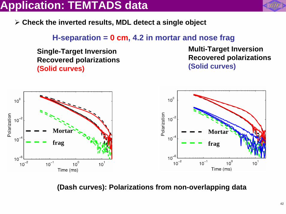
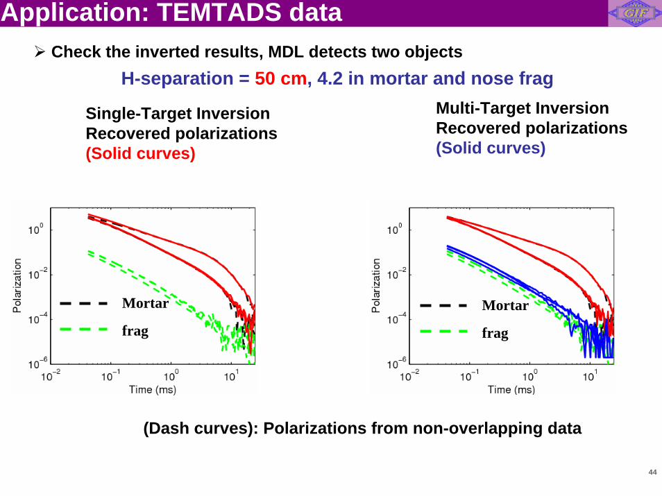
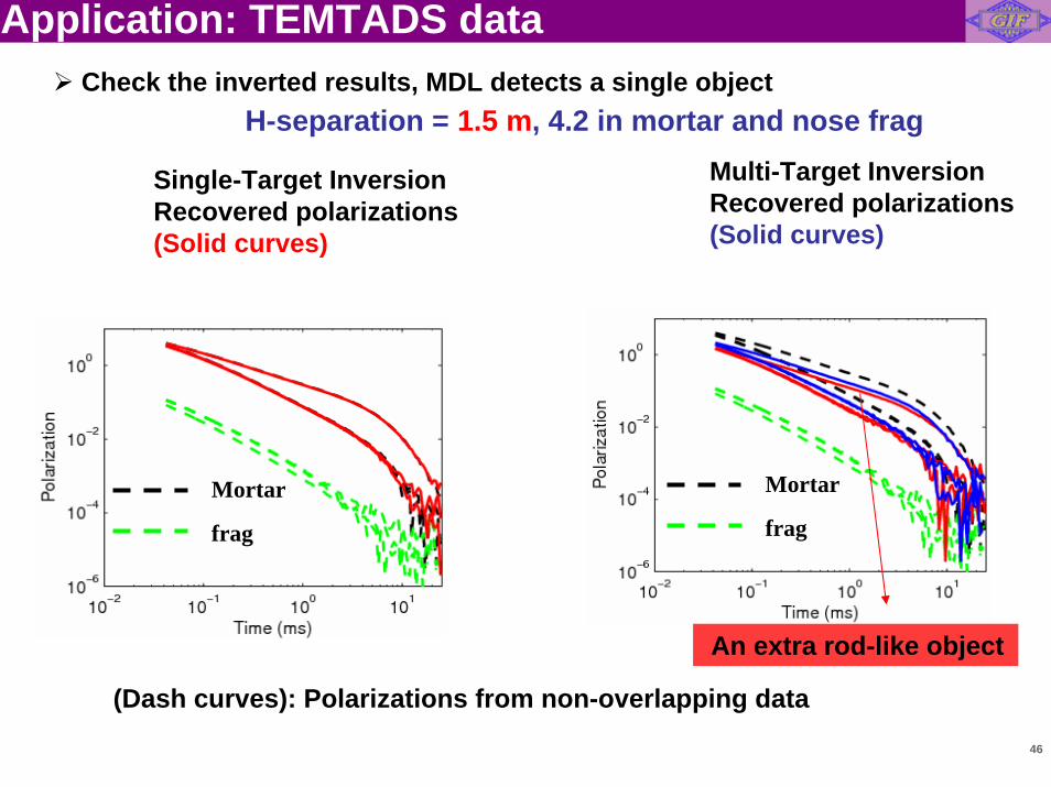
(Dash curves): Polarizations from non-overlapping data
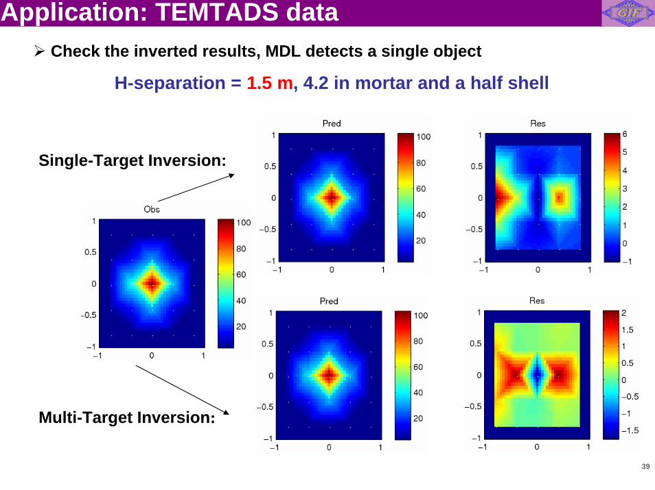
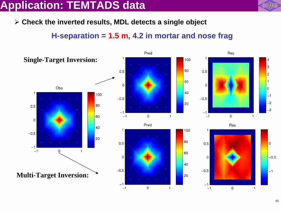
H-separation = 1.5 m, 4.2 in mortar and nose frag
Mortar
frag
Mortar
frag
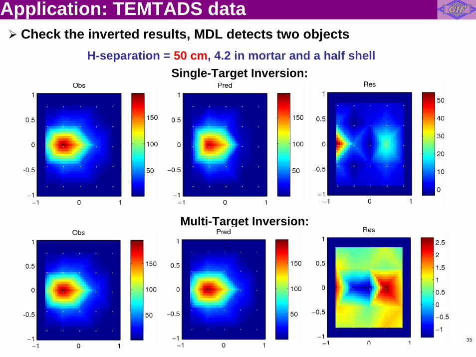
Application: TEMTADS dataCheck the inverted results, MDL detects a single object
An extra rod-like object
47
Future work:
• Any possible improvement in the context of EMI sensing Using a priori available information in the criteriaThresholding sample covariance matrix
Summary
Information-theoretic criteria consider both data fitting and model complexity to estimate source number
• ITC can be implemented in detection-only mode or joint detection-estimation mode.
• Joint detection-estimation mode appears robustrelative to detection-only mode.
48
Acknowledgements
• The work is supported by SERDP MM-1637 project
• We are grateful to Daniel A. Steinhurst and Herb Nelson of NRL and James Kindon and Tomas Bell of SIAC for kindly providing TEMTADSsensor information and data.