Page 1
Wright State University Wright State University
CORE Scholar CORE Scholar
Browse all Theses and Dissertations Theses and Dissertations
2010
Development of an Unsteady Aeroelastic Solver for the Analysis Development of an Unsteady Aeroelastic Solver for the Analysis
of Modern Turbomachinery Designs of Modern Turbomachinery Designs
Timothy James Leger Wright State University
Follow this and additional works at: https://corescholar.libraries.wright.edu/etd_all
Part of the Engineering Commons
Repository Citation Repository Citation Leger, Timothy James, "Development of an Unsteady Aeroelastic Solver for the Analysis of Modern Turbomachinery Designs" (2010). Browse all Theses and Dissertations. 1006. https://corescholar.libraries.wright.edu/etd_all/1006
This Dissertation is brought to you for free and open access by the Theses and Dissertations at CORE Scholar. It has been accepted for inclusion in Browse all Theses and Dissertations by an authorized administrator of CORE Scholar. For more information, please contact [email protected] .
Page 2
Development of an Unsteady
Aeroelastic Solver for the Analysis of
Modern Turbomachinery Designs
A dissertation submitted in partial fulfillment of the
requirements for the degree of
Doctor of Philosophy
By
Timothy James Leger
M.S. Wright State University, 2000
2010
Wright State University
Page 3
WRIGHT STATE UNIVERSITY
SCHOOL OF GRADUATE STUDIES
August 18, 2010
I HEREBY RECOMMEND THAT THE DISSERTATION PREPARED UNDER MY
SUPERVISION BY Timothy James Leger ENTITLED Development of an Unsteady
Aeroelastic Solver for the Analysis of Modern Turbomachinery Designs BE ACCEPTED
IN PARTIAL FULFILLMENT OF THE REQUIREMENTS FOR THE DEGREE OF
Doctor of Philosophy.
________________________________
Mitch Wolff, Ph.D.
Dissertation Director
________________________________
Ramana V. Grandhi, Ph.D.
Director, Ph.D. in Engineering Program
________________________________
Andrew T. Hsu, Ph.D.
Dean, Graduate Studies
Committee on
Final Examination
_______________________________
Mitch Wolff, Ph.D.
_______________________________
Scott Thomas, Ph.D.
_______________________________
Joseph Shang, Ph.D.
_______________________________
Gary Lamont, Ph.D.
_______________________________
David A. Johnston, Ph.D.
Page 4
ii
ABSTRACT
Leger, Timothy James, Ph.D., Department of Mechanical and Material Engineering,
Wright State University, 2010. Development of an Unsteady Aeroelastic Solver for the
Analysis of Modern Turbomachinery Designs
Developers of aircraft gas turbine engines continually strive for greater efficiency
and higher thrust-to-weight ratio designs. To meet these goals, advanced designs
generally feature thin, low aspect airfoils, which offer increased performance but are
highly susceptible to flow-induced vibrations. As a result, High Cycle Fatigue (HCF) has
become a universal problem throughout the gas turbine industry and unsteady aeroelastic
computational models are needed to predict and prevent these problems in modern
turbomachinery designs. This research presents the development of a 3D unsteady
aeroelastic solver for turbomachinery applications. To accomplish this, a well
established turbomachinery Computational Fluid Dynamics (CFD) code called Corsair is
loosely coupled to the commercial Computational Structural Solver (CSD) Ansys®
through the use of a Fluid Structure Interaction (FSI) module.
Significant modifications are made to Corsair to handle the integration of the FSI
module and improve overall performance. To properly account for fluid grid
deformations dictated by the FSI module, temporal based coordinate transformation
metrics are incorporated into Corsair. Wall functions with user specified surface
roughness are also added to reduce fluid grid density requirements near solid surfaces.
To increase overall performance and ease of future modifications to the source code,
Corsair is rewritten in Fortran 90 with an emphasis on reducing memory usage and
Page 5
iii
improving source code readability and structure. As part of this effort, the shared
memory data structure of Corsair is replaced with a distributed model. Domain
decomposition of individual grids in the radial direction is also incorporated into Corsair
for additional parallelization, along with a utility to automate this process in an optimal
manner based on user input. This additional parallelization helps offset the inability to
use the fine grain mp-threads parallelization in the original code on non-distributed
memory architectures such as the PC Beowulf cluster used for this research. Conversion
routines and utilities are created to handle differences in grid formats between Corsair
and the FSI module.
The resulting aeroelastic solver is tested using two simplified configurations.
First, the well understood case of a flexible cylinder in cross flow is studied with the
natural frequency of the cylinder set to the shedding frequency of the Von Karman
streets. The cylinder is self excited and thus demonstrates the correct exchange of energy
between the fluid and structural models. The second test case is based on the fourth
standard configuration and demonstrates the ability of the solver to predict the dominant
vibrational modes of an aeroelastic turbomachinery blade. For this case, a single blade
from the fourth standard configuration is subjected to a step function from zero loading to
the converged flow solution loading in order to excite the structural modes of the blade.
These modes are then compared to those obtained from an in vacuo Ansys® analysis with
good agreement between the two.
Page 6
iv
Table of Contents
Page
ABSTRACT…………………………………………………………………..………...
Table of Contents……………………………………………………………..………...
List of Figures………………………………………………………………..…………
List of Tables………………………………………………………………..………….
List of Symbols................................................................................................................
ii
iv
vi
ix
xi
1. INTRODUCTION…………………………………………………………...………
1.1 Research Objectives……………………………………………..………....
1.2 Literature Review………………………………………………….….…....
1.3 Technical Approach…………………………………………….…….........
1
3
5
13
2. CFD MODEL – CORSAIR…………………………………………….….………...
2.1 Grid Generation…………………………………………………..…………
2.2 Numerical Model……………………………………………….….……….
2.3 Boundary Conditions……………………………………………..………...
15
15
18
38
3. NUMERICAL EVALUATION OF COORDINATE TRANSFORMATION
METRICS………………………………………………………………..…………..
3.1 Recasting in Conservative Form………………………………..…………..
3.2 The Finite Volume Concept……………………………………..………….
3.3 Performance Investigation………………………………………..………...
52
53
55
62
4. WALL FUNCTION.....................................................................................................
4.1 Background Boundary Layer Theory............................................................
4.2 Algebraic Model…………………………………………………..………..
69
70
71
Page 7
v
4.3 Wall Function Model.....................................................................................
4.4 Surface Roughness.........................................................................................
4.5 Test Case........................................................................................................
75
77
81
5. ADDITIONAL PARALLELIZATION…………………………………………..….
5.1 Existing Parallelization in Corsair.................................................................
5.2 Target Computational Platform…………………………………………….
5.3 Code Restructuring…………………………………………………………
5.4 Increased Parallelization……………………………………………………
5.5 Parallel Performance……………………………………………………….
86
86
87
90
95
102
6. FLUID STRUCTURE INTERACTION MODULE…………………………………
6.1 Structural Model Generation.........................................................................
6.2 Mapping…………………………………………………………………….
6.3 Displacement and Load Transfer………………………………….……….
6.4 Information Flow and Time Stepping…………………………….………..
6.5 Conversion of O-grids to Sheared H-grid………………………..…………
116
116
117
119
127
131
7. RESULTS....................................................................................................................
7.1 Rigid Cylinder………………………………………………………………
7.2 Flexible Cylinder with FSI………………………………………………….
7.3 Fourth Standard Modal Analysis…………………………………………...
135
136
141
148
8. SUMMARY AND CONCLUSIONS………………………………………………..
8-1. Suggested Additional Tests & Case Studies................................................
8-2. Further Development & Improvements.......................................................
153
155
157
9. REFERENCES.......……………….………………………………………………… 158
Page 8
vi
Appendix A. Block Tridiagonal Systems………………………………..……………..
Appendix B. Quick Search using Shape Functions…………………………………….
167
169
Page 9
vii
List of Figures
Figure Page
1-1. Sources of unsteady flow in rotating turbomachinery........................................ 2
2-1.
2-2.
2-3.
2-4.
2-5.
2-6
2-7
2-8.
2-9.
Overlaid O-H grid topography............................................................................
Generation of grid extensions for slip boundary condition.................................
Post iterative update for slip boundary condition…………….………………...
Illustration of circumferential periodic condition and ghost points…..………..
Post iterative update of circumferential periodic boundary…………..………..
Section of overlap region between an O-grid and H-grid……………..……….
Simplified view of overlap region between O-grid and H-grid………...……...
Illustration of overlap between an O-grid and clearance grid………………….
Post iterative update of clearance grid collapsing centerline………….……….
18
44
44
46
46
47
48
50
51
3-1.
3-2.
3-3.
Geometry of a finite volume hexahedron cell……………………………….....
Volume swept by a surface ..........………………………………………..…....
Three-dimensional wavy grid……………………………………………..…....
57
59
63
4-1.
4-2.
4-3.
4-4.
Skin friction coefficient as a function of local Reynolds number……………...
Local Reynolds number as a function of surface roughness to grid
height ratio......................................................................................................…
STCF4 flow domain………………………………………………………..….
STCF4 pressure coefficients at mid-span……………………………………...
79
79
83
84
5-1.
5-2.
5-3.
Taylor cluster compute node rack.......................................................................
Taylor cluster network configuration..................................................................
Illustration of three radial overlap points............................................................
89
89
98
Page 10
viii
5-4.
5-5.
5-6.
5-7.
5-8.
Speedup performance..........................................................................................
Parallel efficiency................................................................................................
Average idle times...............................................................................................
Calculation to communication time ratios..........................................................
Maximum nodal memory footprint.....................................................................
110
110
112
112
113
6-1.
6-2.
6-3.
6-4.
6-5.
6-6.
6-7.
6-8
6-9.
6-10.
6-11.
Example mapping at the interface.......................................................................
Area for Gauss quadrature...................................................................................
Conservative transfer of forces...........................................................................
Interpolative transfer of displacements...............................................................
Algebraic deformation of fluid grid points.........................................................
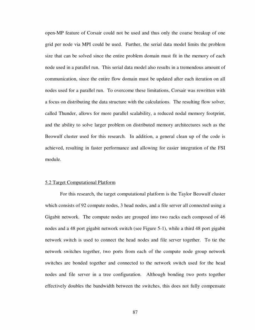
Illustration of anchor points in O-grid topography.............................................
Conventional serial time-staggered algorithm....................................................
Flow of information in FSI module.....................................................................
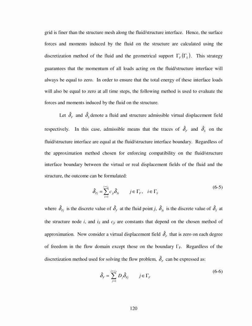
Socket communication........................................................................................
Turbo sheared H-grid topography.......................................................................
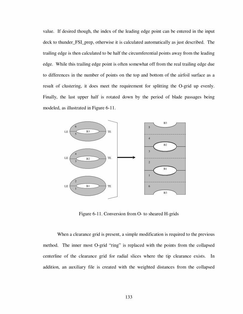
Conversion from O- to sheared H-grids..............................................................
119
123
124
124
125
126
127
130
131
132
133
7-1.
7-2.
7-3.
7-4.
7-5.
7-6.
7-7.
2D midspan slice of channel and cylinder grids.................................................
Close-up of O-grid around the cylinder..............................................................
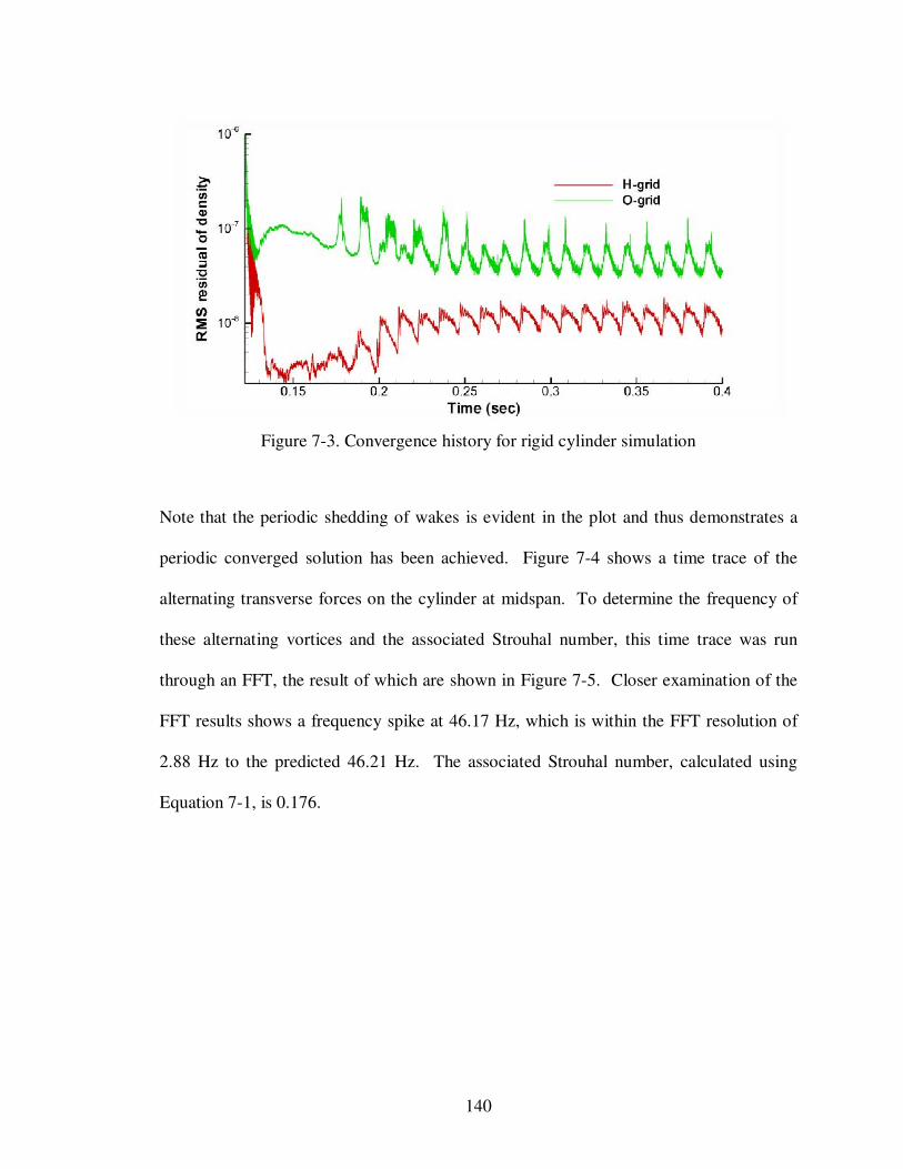
Convergence history for rigid cylinder simulation.............................................
Time trace of transverse forces on cylinder at midspan......................................
FFT of transverse forces on cylinder at midspan................................................
First three mode shapes for the clamped-clamped cylinder................................
Cylinder displacement at midspan......................................................................
138
139
140
141
141
143
145
Page 11
ix
7-8.
7-9.
7-10.
7-11.
7-12.
FFT of transverse and axial displacements at midspan.......................................
Structural mesh for the flexible cylinder.............................................................
Structural mesh for STCF4.................................................................................
Time trace of axial displacement at TE tip.........................................................
FFT of axial displacement at TE tip....................................................................
146
148
149
150
150
B-1.
B-2.
One dimensional linear element..........................................................................
Portion of overlaid O- and H-grid.......................................................................
169
172
Page 12
x
List of Tables
Table Page
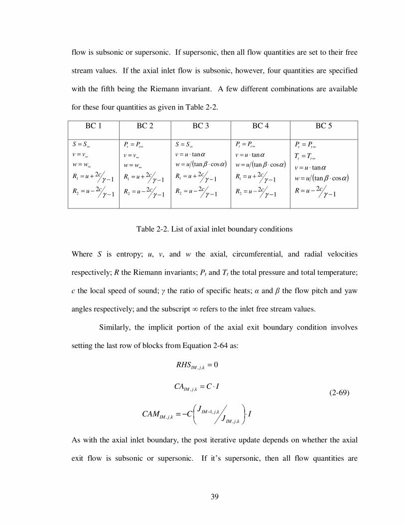
2-2.
2-1.
List of axial inlet boundary conditions................................................................
List of difference schemes for inviscid numerical fluxes....................................
26
39
3-1.
3-2.
Free-stream preservation errors for stationary 3D wavy grid..............................
Free-stream preservation errors for deforming 3D wavy grid.............................
64
65
5-1.
5-2.
5-3.
5-4.
5-5.
Some global information generated by thsplit for each node..............................
Decomposition indexes of example STCF4 grid domain....................................
Runtime and memory usage comparison between Thunder and Corsair............
Parallel performance for split_type of one..........................................................
Parallel performance for split_type of two..........................................................
93
101
103
109
109
7-1. Main vibrational frequencies for STCF4............................................................. 151
Page 13
xi
List of Symbols
Symbol Description
A area
A,B,C flux jacobians
c speed of sound
cp constant pressure specific heat
cv constant volume specific heat
chmp number of Chimera grid points
C Courant number
Cf skin friction coefficient
Ckleb Klebanoff constant
e energy
E efficiency, Young’s modulus
E,F,G flux vectors
f force, frequency (Hz)
flops floating point operations
F force
G serial runtime multiplier
GB gigabyte
h enthalpy
i,j,k,n grid and time indices
in inch
I identity matrix, mass moment of inertia
J Jacobian of coordinate transformation
k thermal conductivity
ks sand roughness height
KB kilobytes
K parallel efficiency constant
l mixing length
lbf pounds-force
L characteristic length
LHS left hand side
m mass
MB megabyte
n normal vector
N shape function
NMF nodal memory footprint
ovlp grid overlap
P pressure, number of processors
P+
nondimensional boundary layer pressure gradient
Pr Prandtl number
q heat flux
Q solution vector
r radius from hub, surface vector
R gas constant, Riemann invariant
Page 14
xii
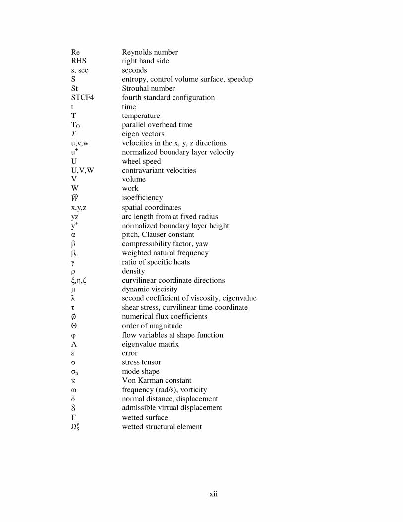
Re Reynolds number
RHS right hand side
s, sec seconds
S entropy, control volume surface, speedup
St Strouhal number
STCF4 fourth standard configuration
t time
T temperature
TO parallel overhead time
T eigen vectors
u,v,w velocities in the x, y, z directions
u+ normalized boundary layer velocity
U wheel speed
U,V,W contravariant velocities
V volume
W work
isoefficiency
x,y,z spatial coordinates
yz arc length from at fixed radius
y+ normalized boundary layer height
α pitch, Clauser constant
β compressibility factor, yaw
βn weighted natural frequency
γ ratio of specific heats
ρ density
ξ,η,ζ curvilinear coordinate directions
µ dynamic viscisity
λ second coefficient of viscosity, eigenvalue
τ shear stress, curvilinear time coordinate
numerical flux coefficients
Θ order of magnitude
φ flow variables at shape function
Λ eigenvalue matrix
ε error
σ stress tensor
σn mode shape
κ Von Karman constant
ω frequency (rad/s), vorticity
δ normal distance, displacement
δ admissible virtual displacement
Γ wetted surface
ΩS wetted structural element
Page 15
xiii
Subscripts
comm communication
F fluid
IM,JM,KM grid index limits
LD long diagonal
P parallel
S serial, structure
t total
TH tetrakis hexahedron
v viscid
wall value at the wall
xcalc calculation of solution
∞ inlet free-stream
Superscripts
‘ pseudo term
+ normalized
~ physical flux
^ numerical flux
total
* non-dimensional term
,
intermediate ADI solutions
F fluid
S structure
Page 16
xiv
ACKNOWLEDGEMENTS
I would like to express my sincere appreciation to my adviser, Dr. Mitch Wolff,
for introducing me to the field of turbomachinery and for the encouragement he has given
me throughout my graduate studies. I feel fortunate and privileged to have worked with
such a dedicated and talented professor. I extend my utmost gratitude and respect to him.
A great deal of thanks also goes to Dr. David Johnston for his insight and help
with this research, especially with regards to the Fluid Structure Interaction module. I
would also like to gratefully acknowledge Dr. Joseph Shang, Dr. Gary Lamont, and Dr.
Scott Thomas for serving on my dissertation committee and providing excellent
classroom instruction.
I am fortunate to have interacted with many bright, talented, and motivated
individuals at Wright State. Special thanks go to Greg Wilt, Sean Mortara, Jonathan
Blair, Dr. Jim Menart, Dr. Ken Cornelius, Dr. George Huang, Dr. Haibo Dong, and all
my instructors, you helped me more than you will ever know.
Finally, I would like to thank my parents, Jim and Verna, for their unwavering
support through times when it looked like I might never graduate. They have been the
greatest influence in my life and I owe all my success to them. Their moral and financial
support throughout my life has given me the ability to be where I am today. I dedicate
this dissertation to them.
Page 17
1
1. INTRODUCTION
Developers of aircraft gas turbine engines continually strive for greater efficiency
and higher thrust-to-weight ratio designs. To meet this goal, the trend in gas turbine
designs has been to reduce size and weight of engines by decreasing the number of
compressor stages, the number of blades per row, and the axial spacing between
vane/blade rows [1]. However, these reductions result in significantly increased
aerodynamic loading of the blades and unsteady interaction between blade rows. In
addition, advanced compressor designs generally feature thin, low aspect airfoils, which
offer increased performance but are highly susceptible to flow-induced vibrations [2]. As
a result, High Cycle Fatigue (HCF) has become a universal problem throughout the gas
turbine industry. In response to these HCF problems, a considerable portion of recent
research in compressor and turbine design has involved the investigation of unsteady
aeroelastic phenomena, namely flutter and forced response [3].
Flutter is defined as an unstable and self-excited vibration of a body in an
airstream and results from a continuous interaction between the aerodynamics and the
structural mechanics, both of which tend to be nonlinear in modern turbomachinery
designs [4]. In turbomachinery blade rows, the mass ratio (structure to fluid) tends to be
high resulting in a single-mode phenomenon. This is because the aerodynamic forces,
which remain much smaller than the inertial and stiffness forces, do not usually cause
modal coupling. However, this also means that the aeroelastic mode can be significantly
Page 18
2
different from the structural mode in both frequency and modal shape. Flutter is a
particularly difficult problem in turbomachinery since there are many additional features
with consequences that are currently not fully understood. These include flow distortions
due to up and down stream blade-rows and the loss of spatial periodicity of vibration due
to aerodynamic effects and blade-to-blade differences (commonly known as structural
and aerodynamic mistuning) [5].
Figure 1-1. Sources of unsteady flow in rotating turbomachinery
When rotating blades pass through flow defects created by the interaction of
upstream and downstream blade rows, the ensuing large unsteady aerodynamic forces can
cause excessive vibration levels. This interaction between blade rows is known as forced
response [4] and becomes a major problem when the excitation frequency coincides with
a natural frequency of the blade. Of particular interest to designers is the prediction of
vibration amplitude under unsteady aerodynamic loading which can be due to wake
passing from upstream blade-rows (wake-rotor interaction), the potential field of
upstream and downstream blade rows (potential-rotor interaction), or to fluctuating back
Page 19
3
pressures [6]. Because of the numerous unknown factors such as structural damping,
nonlinear damping in the blade roots, and the forcing itself, forced response analyses
usually aim at ranking potential designs rather than predicting actual vibration levels.
Current designers typically address HCF and unsteady aeroelastic phenomena
using a Computational Fluid Dynamics (CFD) analysis of a single blade row with the
unsteady forcing applied through specified inflow/outflow boundary conditions or the
predicted blade motion itself [4]. The resulting blade row unsteady loading is utilized
with a Computational Structural Dynamics (CSD) model to determine the unsteady
stresses and the predicted blade fatigue life. While these two steps may be iterated upon
several times, they are usually performed by different groups with an associated loss in
accuracy and efficiency. In addition, the CFD models used are generally inviscid and
time-linearized, resulting in a model that is invalid at off design operating conditions
where serious unsteady aeroelastic problems generally exist in modern turbomachinery
designs [7]. This situation coupled with the inadequate modeling of blade row
interaction, is believed to be the cause for a number of unexpected HCF failures [8,9].
Thus, a computational model which precisely accounts for Fluid Structure Interaction
(FSI), inviscid-viscid interaction, and multi-blade row interaction is needed by designers
to predict HCF and unsteady aeroelastic phenomena of current and future turbomachinery
designs.
1.1 Research Objectives
The goal of this research is to develop an aeroelastic solver for the design of
advanced turbomachinery. However, this lofty goal implies several objectives which
Page 20
4
need to be met in order to achieve such a design tool. First, in order to obtain usable
results, the fluid solver must be capable of handling the deforming fluid grids which arise
from the deformation of the blade. This entails implementing coordinate transformation
metrics (both spatial and temporal) that do not violate the conservation of both surfaces
and volumes under deformation.
Another important objective, in order for this tool to be utilized in the time limited
design environment, is the reduction of solution runtime. This objective is limited to
three main areas in this research for which it can be effectively achieved. The first is to
incorporate a wall function into the chosen flow solver, Corsair [10], to reduce the grid
density required near surfaces for the calculation of shear stresses. By reducing the grid
density near surfaces, the total number of grid points in the computational domain and
thus the simulation runtime is significantly reduced. A second area of focus is to
incorporate additional parallelization via domain decomposition of individual fluid grids
in the radial direction. By dividing the computational domain into pieces and solving
these on separate cores/nodes simultaneously, the simulation runtime is again reduced.
Lastly, a third area involves optimization of the flow solver code itself. While labor and
time intensive, the rewriting/restructuring of older codes (such as Corsair) is often
rewarded with impressive performance improvements, mainly due to the correction of
unobserved bugs/flaws which arise over time via modification of the original source
code.
The final objective for the development of any computational tool is thorough
testing and results. For this research effort, testing against the well understood flexible
cylinder in cross flow is utilized. In addition, the resulting aeroelastic solver is used to
Page 21
5
predict the major vibrational modes of a turbine blade from the fourth standard
configuration.
1.2 Literature Review
A key development in the early understanding of aeroelasticity was made by Lane
who introduced the concept of the interblade phase angle [11]. In this concept, the
individual blades in a cascade are assumed to vibrate with the same amplitude but the
maximum is reached with a constant phase lag, i.e. the interblade phase angle. Armed
with this assumption, the structure and the fluid are decoupled so that a free vibration
problem (taking no account of the aerodynamic loads) can first be solved. The predicted
mode-shapes are then utilized with arbitrary amplitudes to produce prescribed blade
motion. The unsteady fluid problem is then solved with this prescribed blade motion and
the resulting unsteady aerodynamic forces on the blade calculated. These unsteady
aerodynamic forces are then used to measure the stability of the system. This is often
referred to as the classical method and became popular early in computational aerelastic
research for two main reasons [12]. First, assumptions had to be made in order to solve
the complicated differential equations of motions with the limited computing power
available. Second, there has been a tendency to use existing aerodynamic and structural
codes separately with a minimum of changes to either one in order to accommodate the
other.
Although several methods have been developed to measure the stability from the
unsteady aerodynamic forces, the most popular by far has been the aeroelastic
eigensolution method [13]. This method is based on expressing the resulting unsteady
Page 22
6
aerodynamic forces in the frequency domain, either directly if analytical theories are used
or by Fourier analysis if the forces are calculated in the time domain. The resulting
aeroelastic equations of motion are very similar to the structural equations, with the
aerodynamic contributions being added to the mass and/or stiffness matrices. The
stability of the system is then assessed by determining the amount of damping required
for each aeroelastic mode. The main advantage of this method lies in its simplified
representation of the structural dynamics, which allows parametric studies to be
conducted with a minimum of computational effort. Various cascades have been studied
using this technique over the last 30 years, with various simplifications and
improvements to the flow solvers used [14,15,16,17,18].
Integrated aeroelastic methods do not uncouple the fluid motion from that of the
structure, but instead treat the problem of aeroelasticity in one continuous medium. The
need for such an approach arises from the nonlinear response of the fluid flow to the
motion of solid boundaries, especially in the transonic regime where flutter often occurs.
Hence, the resulting mathematical formulation must allow the fluid to modify the
structural motion and vice-versa, as such phenomena occur in nature. It then becomes
possible to include nonlinear effects for both the fluid and the structure and take into
account various interactions that can take place between them. The most striking
difference between the classical method and the integrated method is that the former can
only predict the onset of flutter as a sudden change from a stable to an unstable region
while the latter is capable of predicting limit-cycle behavior. The engineering value of
such prediction methods is evident since there is enough experimental evidence to
suggest that flutter occurs in pockets of the limit cycle with varying amplitude levels [4].
Page 23
7
This observation has a crucial implication on flutter analyses. The prediction of flutter
onset may not be as important as predicting the actual vibration amplitude, since limit
cycles can be tolerated if their amplitude is small.
Early integrated aeroelastic models typically incorporated an inviscid 2D Euler
solver with an extremely simplified linear structural model consisting of springs, masses,
and dampeners [14,19,20,21,22]. While the airfoil was allowed to move in response to
aerodynamic forces and moments, the airfoil shape was kept rigid. In addition, many of
these early models were restricted to a two-degrees-of-freedom structural model (pitch
and plunge). These models have been extensively used in past research to determine the
so-called flutter bucket or the reduced speed at which flutter occurs. However, due the
extremely simplified structural models used, these early efforts are also commonly
referred to as a classical method [4].
While studies using both these classical methods have provided important first
steps in the prediction of unsteady aeroelastic phenomena, they lack the nonlinear
response of the structure and thus the complete flow physics resulting from FSI [7].
Thus, recent efforts in the area of aeroelastic CFD research has involved the coupling of
fluid and structural solvers, where both solvers are capable of handling full nonlinear
effects, such as those that occur in transonic turbomachinery. Different strategies can be
used to obtain a solution of the coupled fluid structure system. The first possibility is to
use a strong coupling, sometimes referred to as a fully integrated method, where the
structural and fluid dynamics equations are solved together at each time step using the
same integrator. This is done by discretizing the two domains into one Arbitrary
Lagrangian-Eulerian (ALE) space, the result of which is that the motion of the grid
Page 24
8
becomes an integral part of the equations of motion and does not have to be handled
separately [23].
Bendiksen [24] applied a direct version of this method to both wing and
turbomachinery blade flutter. His method used an explicit temporal discretization which
is integrated using a five-stage Runge-Kutta scheme, with upwind differencing used for
the spatial discretization of the arbitrary Lagrangian-Eulerian formulation. The structural
equations are formulated on a local node level which enables them to be discretized using
the same five-stage Runge-Kutta integrator. This model is claimed to calculate the
energy transfer between the structure and fluid more accurately than similar schemes.
For the flutter analysis, a typical isolated wing section was modeled, with the section
allowed to have camber bending. This chord wise flexibility was modeled using plate-
type finite elements of unit width. Results from this case were compared to those from
classical methods showing excellent agreement. In addition, the results suggest that
camber bending plays an important role in transonic flutter, possibly due to the mixed
subsonic-supersonic flow field being sensitive to the airfoil boundary condition in the
supersonic region of the flow. Calculations were also made on a cascade with solid
titanium blades. This case demonstrated that camber bending can reach significant
amplitudes during transonic flutter of thin compressor blades.
Masud [25] developed a space-time finite element formulation of the Navier-
Stokes equations that was stabilized using the Galerkin/least-squares approach. The
variational equation was based on the time discontinuous Galerkin method and was
written in terms of physical entropy variables over the moving and deforming space time
slabs. This formulation thus becomes analogous to the ALE formulation discussed
Page 25
9
previously including viscous effects. To demonstrate the versatility of this method,
numerical simulations of a projectile moving in a stationary flow field were presented.
Gottfried and Fleeter [23,26] extended ALE3D, a 3D finite element Euler solver,
to model the unsteady aerodynamics of stator-rotor interaction in turbomachinery.
Simulations of a transonic compressor at Purdue University with the code, renamed
TAM-ALE3D, showed good prediction of both subsonic and transonic steady state
conditions. However, the simulation over-predicted the unsteady IGV lift magnitude by
100% for the subsonic case. In the transonic case, the simulated IGV lift lacked the
higher harmonic content of the experimental data. The discrepancies between
experimental and simulated results were attributed to scaling of the geometry and the lack
of viscous effects.
Sadeghi and Liu [27] investigated the effects of frequency mistuning on cascade
flutter using a similar ALE formulation. The unsteady structural and Euler equations
were simultaneously integrated in time. A second order accurate implicit finite-volume
scheme was used to solve both the flow equations and structural model. Using this
model, simulations were performed for a turbine cascade with flutter in the bending mode
and with alternate mistuning of the structural eigen frequency. An important finding of
this study was that the fluid-structure interaction tended to decrease the effective amount
of mistuning. Along similar lines, it was discovered that a minimum amount of
mistuning was required to stabilize the cascade. Similar behavior was demonstrated for a
compressor cascade.
While closely-coupled methods show promise, the approach requires an enormous
amount of computational power along with almost a complete rewrite of the solver.
Page 26
10
Additionally, the matrix system for the coupled problem is in general ill-conditioned as a
result of the difference in stiffness of the fluid and the solid. A more reasonable approach
is to use a loosely coupled method. In this method, the fluid and solid variables are
updated alternatively by independent CFD and CSD codes which exchange boundary
information at each time step in a time accurate manner. The most attractive feature of
this approach is that the CFD and CSD solvers are largely independent of one another.
This allows efficient re-use of codes that have been developed over several years and
have been extensively tested. In addition, different fluid and structural models can be
interchanged according to the requirements of a particular application. For example,
CFD solvers for modeling transonic flow are very different from those used for the
hypersonic regime. Likewise, different CSD models exist for types of structures, ranging
from metal matrices to composites and even nanostructures [28].
Srivastava et al. [29] developed an efficient three-dimensional hybrid scheme by
loosely coupling an ADI Euler solver with the commercial CSD package NASTRAN to
analyze two advanced propeller designs. Their scheme treated the spanwise direction
semi-explicitly and the other two directions implicitly. They noted that accuracy when
compared to a fully implicit scheme was not affected, while providing advantages of
reduced computational requirements in both memory and time. The calculated power
coefficients for the advanced designs at various operating conditions showed good
correlation with experimental data and varied up to 40% from CFD simulations run
without aeroelastic deformation. Spanwise distribution of elemental power coefficients
and steady pressure coefficient differences were in good agreement with experimental
data. However, their study also uncovered that adjustments to the setting angle by rigid-
Page 27
11
body rotation did not simulate the correct blade shape. A follow up study by Yamamoto
et al. [30] of the effect of structural flexibility on the performance of these propeller
designs showed that structural deformation due to centrifugal and steady aerodynamic
loading were important for improved correlation to experimental data. In addition, it was
noted that structural deformation from unsteady aerodynamic forces played a key role in
the performance of the designs.
Sayma et al. [31] developed a model for forced response prediction in
turbomachinery blades. Their three-dimensional multi-passage, multi-blade-row
calculations coupled both the fluid and the structure through an exchange of boundary
conditions at every time step. The structure was represented by a linear modal model
obtained from a standard FEA formulation, while the flow analysis was performed using
a three-dimensional time-accurate viscous model using unstructured grids. Variables
were interpolated at the sliding boundaries between the rotor and the stator in a
conservative manner in order to allow a free movement of discontinuities. This model
was used to study an intermediate pressure turbine in order to rank the magnitude of the
fluid forcing resulting from two types of nozzle guide vanes. A sector of one stator and
five rotor blades was analyzed for both types of nozzle guide vanes and the results
obtained showed good agreement with available experimental data.
Vahdati et al. [32] used the same model to predict both the blade passing and low
engine order forced response of a low pressure turbine. The predicted force response
vibration amplitudes for a 24 nodal diameter resonance were found to be in good
agreement with measured data but one of the main uncertainties was identified as the
determination of the inherent mechanical damping. In addition, use of a whole-annulus
Page 28
12
2-row model showed that non-uniform spacing of the stator blades gave rise to low
engine order excitation. Breard et al. [33] also used this same model to perform a flutter
analysis of a complete civil aero-engine fan assembly for three different configurations:
no intake, symmetric intake, and non-symmetric flight intake. The blade’s dynamic
behavior was found to be different for each of these configurations, demonstrating the
influence of intake ducts on flutter stability.
Servera et al. [34] investigated the use of a loose coupling between a CSD model
for the analysis of helicopter rotor blades called HOST, and an Euler solver for
computing the trim of flexible rotors in steady forward flight called WAVES. This
coupling was used to analyze two advanced helicopter rotor designs and showed that a
simultaneous coupling of the lift, pitching moment, and drag parameters is required in
order to obtain a converged solution independent of simplified aerodynamic models. In
addition, the coupled model showed significant improvements on the pitching moment
and torsion predictions.
Carstens et al. [35] compared results from a loosely-coupled algorithm of a low
pressure compressor at design conditions to those from a classical analysis using LIN3D.
to those from a classical analysis using LIN3D of a low pressure compressor at design
conditions The structural model consisted of an FEA model time-integrated using the
Newmark algorithm, while the unsteady aerodynamics were computed using a Navier-
Stokes code. An automatic grid generator was used to dynamically deform the mesh and
couple the two codes together. This model was then used to analyze an assembly of
highly loaded compressor blades in transonic flow. They found that the loosely-coupled
algorithm yielded lower aerodynamic damping over the full range of interblade phase
Page 29
13
angles, unlike the classical LIN3D analysis. A striking result of the coupled algorithm
was the negative damping for an interblade phase angle of 0, which might cause self-
excited vibrations if no structural damping were present to keep the system stable.
1.3 Technical Approach
An aeroelastic computational model is built from an existing, well-developed
ideal-gas, compressible, turbomachinery flow solver called Corsair. To account for the
deformations from unsteady aerodynamic loadings, Corsair is loosely coupled to the
commercial CSD code Ansys® through the use of a general FSI module [36]. This
general FSI module handles the calling and setup of the CSD model, conversion of
surface fluid stresses to structural forces, time stepping of the CSD model, and morphing
of the fluid grid to match deformations predicted by the CSD model. By using this
general FSI module, the resulting CFD – CSD coupling remains flexible and can take
advantage of utilizing different CSD models.
To accomplish the CFD – CSD coupling, significant modifications to Corsair
were required. Improved methods for numerical evaluation of the coordinate
transformation metrics to handle grid deformations introduced by the FSI module are
studied. The optimal methods for the spatial and temporal metrics from this study are
then used in Corsair for the remaining research. A wall function with user specified
surface roughness is also implemented into Corsair, allowing a significant reduction in
grid density requirements for accurate prediction of shear stresses along solid surfaces.
Following the implementation and verification of the wall function, an investigation is
performed comparing the wall function against the finite difference approach used in the
Page 30
14
current release of Corsair to gauge performance differences and accuracy. To reduce
simulation runtimes on non-SMP super-computers such as PC Beowulf clusters[37], the
common data model used in Corsair is converted to a distributed data model resulting in a
much smaller per nodal memory footprint. This change lead to a complete rewriting and
restructuring of the source code, the result of which is called Thunder. To increase
parallelization, radial decomposition of individual grids is also implemented into solver.
A utility to optimize the decomposition of each grid is created, requiring only the number
of pieces each grid is to be broken into to be specified by the user. Comparisons are then
made between the original version of Corsair and the improved model called Thunder to
demonstrate parallel scalability, performance, and reduction in nodal memory
requirements.
To test the FSI model, two simplified configurations are utilized. First, the well
understood case of a flexible cylinder in cross flow is studied with the natural frequency
of the cylinder set to the shedding frequency of the Von Karman Streets. The cylinder is
self excited, demonstrating the exchange of energy between the fluid and structural
models. The second test case is based on the fourth standard configuration and
demonstrates the ability of the FSI model to predict the dominant vibrational modes of an
aeroelastic turbomachinery blade. For this case, a single blade from the fourth standard
configuration is subjected to a step function from zero loading to the converged flow
solution loading in order to excite the structural modes of the blade. These modes are
then compared to those obtained from an in vacuo analysis using Ansys®.
Page 31
15
2. CFD MODEL – CORSAIR
Before any of the required modifications to the flow solver chosen for this
research could be made, especially to the structure of the code itself, a somewhat detailed
understanding of the solution methods employed in Corsair was first required. Since no
other publications or sources for Corsair exist with the needed level of detail, the source
code itself was painstakingly analyzed and documented. This chapter is the result of that
effort and provides a detailed look at the solution method employed by Corsair, including
grid generation, numerical formulation, and boundary conditions.
The unsteady aeroelastic solver developed in this research is based on a well
established turbomachinery CFD code called Corsair [10], distributed by the NASA
Marshal Space Flight Center. Corsair is a three-dimensional Reynolds Averaged Navier
Stokes (RANS) flow solver for axial turbomachinery geometries. It uses an overset
structured grid topography consisting of O-grids around blades and H-grids for passages.
In addition, a clearance grid composed of an O-grid with a collapsed centerline, can be
used in the outer tip of an O-grid to include tip clearance flows in simulations.
2.1 Grid Generation
The first step in using any CFD model is to generate a set of grids over which the
solution will be solved. Corgrid is a three-dimensional structured zonal-grid generator
specifically designed for use with Corsair. A set of overlaid O- and H-grids are generated
Page 32
16
for each blade being modeled at constant radial span-wise locations. Algebraically
generated H-grids are used in the regions upstream of the leading edge, downstream of
the trailing edge, and in the inter-blade region. O-grids, which are body fitted to the
surface of the blade airfoil, are used to properly resolve the viscous flow in the blade
passages and are generated using an elliptic equation solver. As with most grid
generation packages, grids can be clustered around areas of high curvature and near the
hub, shroud, and blade surfaces. For blades with a tip clearance, a second O-grid is
generated using a collapsed center-line to fill in the gap.
Construction of the algebraically generated H-grids begins with the calculation of
the airfoil mean camber line. The mean camber line is extended upstream of the airfoil
leading edge and downstream of the airfoil trailing edge using decay functions to control
the incremental changes in the axial and circumferential spacing. Half the blade pitch is
added to and subtracted from every computational grid point along the extended camber
line to form the first and last grid lines in the blade-to-blade direction. Computational
grid lines are then added at equal spatial increments between the first and last grid lines in
the blade-to-blade direction. In addition, grid lines can be clustered in both the axial and
circumferential directions upstream of the airfoil leading edge and downstream of the
airfoil trailing edge.
Generation of the O-grids begins with the specification of four points on the H-
grid which define a box that delineates the outer boundary of the O-grid. This outer
boundary is smoothed to eliminate discontinuities in the slope of the grid lines at the
corners of the box. The inner boundary of the O-grid is simply the surface of the airfoil.
Page 33
17
An elliptical solution procedure is then used to produce a nearly orthogonal grid [38].
The elliptic equations are:
( )ηξηηξηξξ γβα QxPxJxxx +−=+− 22 (2-1)
( )ηξηηξηξξ γβα QyPyJyyy +−=+− 22 (2-2)
where
22
ηξα yx += (2-3)
ηξηξβ yyxx += (2-4)
22
ξξγ yx += (2-5)
Here, x, y, and z are the Cartesian coordinates and subscripts ξ, η, and ζ are the
curvilinear (or body fitted) coordinates in the axial, radial, and circumferential directions
respectively and represent derivatives in those directions, J is the Jacobian matrix of
curvilinear coordinate transformation, P and Q are forcing functions used to control the
computational point clustering and orthogonality near solid walls. Equations 2-1 and 2-2
are solved using a successive line over-relaxation technique.
To define the overlap region between the O- and H-grids, a second set of four
points on the H-grid are specified which form a box inside the outer boundary of the O-
grid and define the inner boundary of the H-grid. The points inside the inner boundary of
the H-grid are treated as i-blanked points, i.e. the equations of motion are not solved at
these points. However, in the overlap region between the two boxes, the equations of
motion are solved on both the O- and H-grids. Increasing the amount of overlap between
the O- and H-grids enhances the stability and accuracy of the flow solution, but also
Page 34
18
increases the computational time by increasing the number of redundant grid points in the
calculation. A typical overlaid O-H grid is illustrated in Figure 2-1.
Figure 2-1. Overlaid O-H grid topography
2.1 Numerical Model
Corsair is a three-dimensional, implicit, multi blade row flow solver designed for
time accurate simulations of turbomachinery [39]. It utilizes a dual-time-step to solve the
full, unsteady, Navier-Stokes equations in a time accurate manner by means of a
linearized, approximately factored, upwind finite-difference scheme. The resulting
solution is third order spatial and second order temporal accurate. The integration
scheme begins with the three-dimensional unsteady Navier-Stokes equations in strong-
conservation dual-time-step form:
Page 35
19
v
z
v
y
v
xzyxtt GFEGFEQQ ++=++++ ' (2-6)
where t represents the physical time step and t’ represents the pseudo-time step for
subiterations.
The vector of conservative variables Q, the inviscid flux vectors E F G, and the
viscid flux vectors Ev F
v G
v, are given by:
( ) ( ) ( )
+
+
=
+
+=
+
+
=
=
wpe
wP
vw
uw
w
G
vpe
uw
vP
uv
v
F
upe
uw
uv
up
u
E
e
w
v
u
Q
tttt
2
2
2
ρ
ρ
ρ
ρ
ρ
ρ
ρ
ρ
ρ
ρ
ρ
ρ
ρ
ρ
ρ
ρ
(2-7)
=
=
=
z
zz
zy
zx
v
y
yz
yy
yx
v
x
xz
xy
xx
v GFE
β
τ
τ
τ
β
τ
τ
τ
β
τ
τ
τ
000
and the stress tensor is defined by:
( ) ( )( ) ( )
( ) ( )
zzyyxx
zzzzyzxz
yyzyyyxy
xxzxyxxx
yzzyyzyzzyxzzz
xzzxxzxzzyxyyy
xyyxxyxyzyxxxx
kTqkTqkTq
qwvu
qwvu
qwvu
wvwvuw
wuwvuv
vuwvuu
===
+++=
+++=
+++=
=+=+++=
=+=+++=
=+=+++=
τττβ
τττβ
τττβ
ττµτλµτ
ττµτλµτ
ττµτλµτ
2
2
2
(2-8)
with Stokes hypothesis and the perfect gas law completing the equations of motion:
Page 36
20
( )( )
vp
v
p
t
ccRc
c
Peh
R
PT
Pe
wvuee
−==
+==
−=
+++=
−=
γ
ρργρ
ρρ
µλ
12
32
222
(2-9)
By defining the Prandtl number as
k
c pµ=Pr
(2-10)
the heat flux terms in the conservation of energy equation are rewritten as
zzyyxx eqeqeq 111 PrPrPr −−− === γµγµγµ (2-11)
In Corsair, the equations of motion are non-dimensionalized so that certain
parameters, such as the Reynolds number, can be varied independently. The non-
dimensional variables used are as follows:
( )
( ) TTP
PP
c
UU
P
vv
cL
tt
L
xx
====
=
===
∞∞
∞
∞
∞
****
****
ρ
ρρ
γ
µ
µµ
ργ
(2-12)
where x is a distance, L is the mid-span length in the first blade row, t is time, v is a
velocity component, c is the free stream speed of sound, γ is the ratio of specific heats, µ
is the viscosity, U is the wheel velocity, P is the static pressure, ρ is the density, T is
temperature (in degrees Rankine), and the subscript ∞ refers to free stream conditions.
Applying this to Equation 2.6, the equations of motion are rewritten as:
( )
( )v
z
v
y
v
xzyxttGFEGFEQQ ********
1
'Re ++=++++ −
(2-13)
where the non-dimensionalized Reynolds number is given by:
Page 37
21
γµ
ρ
∞
∞=Lc
Re
(2-14)
For the analysis of arbitrary geometries it is useful to generalize the equations of
motion by expressing them in terms of body-fitted, curvilinear coordinates. The
following independent variable transformation introduces body-fitted coordinates which
allow accurate implementation of surface boundary conditions, since the geometric
surface lies along a boundary of the computational domain:
( ) ( ) ( )tzyxtzyxtzyxt ,,,,,,,,, ςςηηξξτ ====
(2-15)
Applying these to Equation 2-13, the equations of motion now take the following form:
( )vvvGFEGFEQQ ςηξςηξττ ++=++++ −1
' Re~~~~~
(2-16)
where
( ) ( )( ) ( )( ) ( )( ) ( )( ) ( )( ) ( ) JGFEG
JGFEF
JGFEE
JGFEQQG
JGFEQQF
JGFEQQE
JQQ
v
z
v
y
v
x
v
v
z
v
y
v
x
v
v
z
v
y
v
x
v
zyxt
zyxt
zyxt
/~
/~
/~
,~
,~
,~
~
***
***
***
****
****
****
ςςςς
ηηηη
ξξξξ
ςςςςς
ηηηηη
ξξξξξ
++=
++=
++=
+++=
+++=
+++=
=
(2-17)
and the metrics of transformation are:
Page 38
22
( ) ( ) ( )( ) ( ) ( )( ) ( ) ( )
( ) ( ) ( )[ ]( ) ( ) ( )[ ]( ) ( ) ( )[ ]
( ) ( ) ( )ξηηξςξςςξηηςςηξ
ηξξητξηηξτηξξητ
ξςςξτςξξςτξςςξτ
ςηηςτηςςητςηηςτ
ξηηξηξξηξηηξ
ςξξςξςςξςξξς
ηςςηςηηςηςςη
ς
η
ξ
ςςς
ηηη
ξξξ
zyzyxzyzyxzyzyxJ
yxyxzzxzxyzyzyxJ
yxyxzzxzxyzyzyxJ
yxyxzzxzxyzyzyxJ
yxyxJzxzxJzyzyJ
yxyxJzxzxJzyzyJ
yxyxJzxzxJzyzyJ
t
t
t
zyx
zyx
zyx
−+−−−=
−+−+−=
−+−+−=
−+−+−=
−=−=−=
−=−=−=
−=−=−=
−1
(2-18)
Application of a second order central approximation for physical time and a first
order backward approximation for pseudo time to Equation 2-16 gives the general
implicit formulation used in Corsair to solve the equations of motion:
( ) ( )( ) ( ) ( )[ ]1111
111,11,1
'11
21,1
231
~~~Re
~~~~~~~2
~
+++−
++++++
∆
−+
∆
++=
+++−++−
nvnvnv
nnnknknnnkn
GFE
GFEQQQQQ
ςηξ
ςηξττ
(2-19)
In Equation 2-19, n denotes a physical time step and k denotes a pseudo time step. While
a second order accurate difference is required for the physical time in order for the
method to be time accurate, a first order difference is sufficient for pseudo time steps,
since the solution is iterated in pseudo time to convergence at each physical time step.
Note that Equation 2-19 is non-linear. To solve the equations of motion in an
efficient computational manner, linearization in the form of a Taylor series expansion
with use of the pseudo time step, τ’, is utilized:
Page 39
23
( ) ( ) ( ) ( )
( ) ( ) ( ) ( )
( ) ( ) ( ) ( ) '
1
'
1
'
1
'
1
'
1
'
1
~~ˆ~~
~ˆ~
~~ˆ~~
~ˆ~
~~ˆ~~
~ˆ~
~~ˆ~~
~ˆ~
~~ˆ~~
~ˆ~
~~ˆ~~
~ˆ~
τςςςςς
τηηηηη
τξξξξξ
τςςςςς
τηηηηη
τξξξξξ
QCGQQ
GGG
QBFQQ
FFF
QAEQQ
EEE
QCGQQ
GGG
QBFQQ
FFF
QAEQQ
EEE
nvn
vv
nvnv
nvnvv
nvnv
nvn
vv
nvnv
nnnn
nnnn
nnnn
∂+∂≈∆
∂
∂∂+∂≈
∂+∂≈∆
∂
∂∂+∂≈
∂+∂≈∆
∂
∂∂+∂≈
∂+∂≈∆
∂
∂∂+∂≈
∂+∂≈∆
∂
∂∂+∂≈
∂+∂≈∆
∂
∂∂+∂≈
+
+
+
+
+
+
(2-20)
where as before, a first order backward difference is used for the pseudo time step:
( )knkn QQQ ,11,1
'
1'
~~~ +++
∆−=
ττ
(2-21)
In Equation 2-20, the quantities ,~
,~
,~
,~
,~ vv BACBA and v
C~
are referred as flux jacobians,
while the quantities ,ˆ,ˆ,ˆ,ˆ,ˆ vv FEGFE and vG , are referred to as numerical fluxes and are
consistent with the physical fluxes ,~
,~
,~
,~
,~ vv FEGFE and v
G~
. Since the solution is
iterated to convergence at each physical time step, error introduced by the linearization
process is eliminated. However, the resulting formulation does require the storage of the
solution at three previous time steps, two at a previously converged physical time step
and one at the previous pseudo time step. Substituting Equations 2-20 into Equation 2-19
and rearranging terms results in:
Page 40
24
( ) ( ) ( )[ ]( ) ( )
( ) ( ) ( )
∂+∂+∂−∂+∂+∂+
+−−=−
∂−∂+∂−∂+∂−∂+
−
−+
∆∆+++
−−−
nv
nv
nvnnn
nnknknkn
vnnvnnvn
GFEGFE
QQQQQ
CCBBAAI
ςςηηξξςηξ
ττ
ςςηηξξ
ˆˆˆReˆˆˆ
~~2
~~~
~Re
~~Re
~~Re
~
1
1
21,1
23',11,1
111
(2-22)
The implicit formulation of a 3-D equation, such as those in Equation 2-22, would
normally result in a system of equation with a hepta-diagonal coefficient matrix. The
solution of such a system, even with re-ordering techniques, is very time consuming and
computationally expensive. To overcome this difficulty, Approximate Factorization (AF)
along with the Alternating Direction Implicit (ADI) algorithm is used in Corsair. The AF
reduces the hepta-diagonal coefficient matrix system to three tri-diagonal systems which
are then sequentially solved using the ADI algorithm. The resulting solution method
requires considerably less computational expense and is unconditionally stable. Since AF
is applied to the LHS of Equation 2-22, the use of pseudo time steps to converge the
solution at each physical time step reduces error caused by both the linearization and AF
techniques together. In practice, three pseudo iterations are sufficient to reduce these
errors down to machine zero. Different factorizations can be used in the AF technique,
resulting in various orders of accuracy and computational expense. The most important
rule of AF is to keep the factorization error (generation of extra terms) below the order of
truncation for the desired solution while preserving existing terms. In Corsair, a fairly
straight forward AF is used:
Page 41
25
( )[ ] ( )[ ] ( )[ ]( ) ( )
( ) ( ) ( )
∂+∂+∂−∂+∂+∂+
+−−=−
∂−∂+∂−∂+∂−∂+
−
−+
∆∆+++
−−−
nv
nv
nvnnn
nnknknkn
nvnnvnnvn
GFEGFE
QQQQQ
CCIBBIAAI
ςςηηξξςηξ
ττ
ςςηηξξ
ˆˆˆReˆˆˆ
~~2
~~~
~Re
~~Re
~~Re
~
1
1
21,1
23',11,1
111
(2-23)
In Equation 2-23, all the fluxes are evaluated explicitly using the solution vector
at the current pseudo time step, knQ ,1~ + . For the inviscid numerical fluxes on the RHS,
Roe’s approximate Reiman solver scheme is utilized. This method accelerates the
solution by taking advantage of the characteristics (propagation direction of information)
of the equations of motion. In Corsair, Roe’s scheme is given by:
( )[
]−+
−+
−
+−
+++
++++∆
∆−∆−∆+
∆−∆−∆+
∆−∆−−=∂
kjikjikji
kjikjikji
kjikjikjikjikji
EEE
EEE
EEEEE
,,23,,12,,1
,,13,,2,,11
,,,,1,,,,11
,,ˆ
φφφ
φφφ
ξξ
(2-24)
for the interior points and by:
( )( )[ ][ ]−−
+++
+
++++∆
∆+∆−∆−∆−+
∆−∆−−=∂
iiii
kjikjikjikjikji
EEEE
EEEEE
110
,,,,1,,,,11
,,
5,max91125.0
ˆ
φ
ξξ
(2-25)
for the second and imax-1 points. Note that Equation 2-25 is a modified second order
accurate formulation of Roe’s scheme. In Equations 2-24 and 2-25, the + and – indicate
contributions from downstream and upstream traveling characteristic waves respectively,
where E represents the total flux given by:
Page 42
26
( )( )( )( )
( )( )
−++++
++++
++++
++++
+++
=
PPewvu
Pwvuw
Pwvuv
Pwvuu
wvu
E
tzyxt
zzyxt
yzyxt
xzyxt
zyxt
ξξξξξ
ξξξξξρ
ξξξξξρ
ξξξξξρ
ξξξξρ
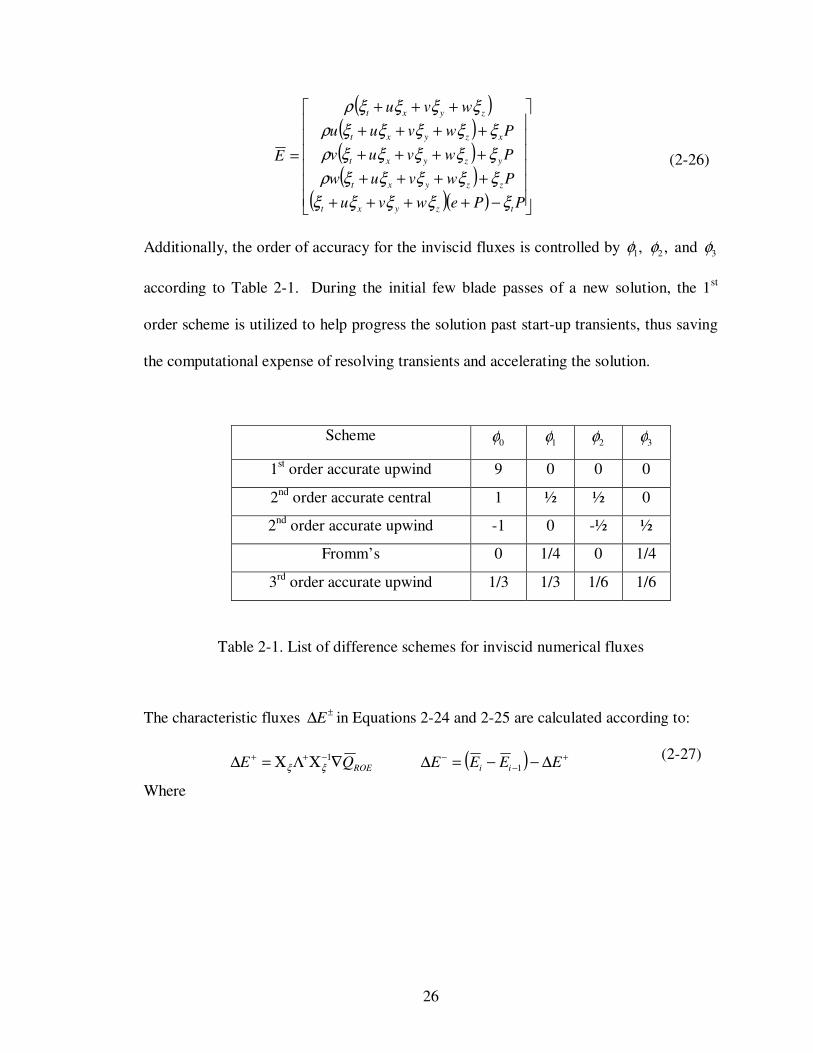
(2-26)
Additionally, the order of accuracy for the inviscid fluxes is controlled by ,, 21 φφ and 3φ
according to Table 2-1. During the initial few blade passes of a new solution, the 1st
order scheme is utilized to help progress the solution past start-up transients, thus saving
the computational expense of resolving transients and accelerating the solution.
Scheme 0φ 1φ 2φ 3φ
1st order accurate upwind 9 0 0 0
2nd
order accurate central 1 ½ ½ 0
2nd
order accurate upwind -1 0 -½ ½
Fromm’s 0 1/4 0 1/4
3rd
order accurate upwind 1/3 1/3 1/6 1/6
Table 2-1. List of difference schemes for inviscid numerical fluxes
The characteristic fluxes ±∆E in Equations 2-24 and 2-25 are calculated according to:
( ) +−
−−++ ∆−−=∆∇ΧΛΧ=∆ EEEEQE iiROE 1
1
ξξ (2-27)
Where
Page 43
27
( ) ( ) ( )
−−−
−+
+++
−+
+
−
+
−
+
−
−++−
−+−+
−++−
=Χ
zyxzyxz
xy
y
zxyz
zzzxyyx
yyxzyzx
xxyzzyx
zyx
wvu
c
c
U
wvu
c
c
U
U
vu
U
uw
U
wv
c
w
c
wwww
c
v
c
vvvv
c
u
c
uuuu
cc
ξξξ
γ
ξξξ
γξ
ξξ
ξ
ξξ
ξ
ξξ
ξξξξξξξ
ξξξξξξξ
ξξξξξξξ
ξξξ
ξ
1212222
22222
22222
22222
11222
(2-28)
( ) ( )
( ) ( )
( ) ( )
( ) ( ) ( )
( ) ( ) ( )
−
−
−
−
−
=
−−−
−−
−−
−−
=
−
−
−
−
−
−−−
−−−
−−
−−
−−
−
∇
Χ
1
1
1
1
1
111
111
11
11
11
1
10
10
10
10
10
ii
ii
ii
ii
ii
ROE
iiziiyiix
iiziiyiix
ziixiiyz
yiixiizy
xiiyiizx
PP
ww
vv
uu
c
c
c
c
c
Q
ρρ
ρρξρρξρρξ
ρρξρρξρρξ
ξρρξρρξξ
ξρρξρρξξ
ξρρξρρξξ
ξ
(2-29)
(2-30)
( )( )UhcwvuUhh
h
www
vvv
uuu
ii
iiii
ii
iiii
ii
iiii
ii
iiii
zyx
zz
zyx
y
y
zyx
xx
21222
1
11
1
11
1
11
1
11
222222222
1 −−=++=+
+=
+
+=
+
+=
+
+=
++=
++=
++=
−
−−
−
−−
−
−−
−
−−
γρρ
ρρ
ρρ
ρρ
ρρ
ρρ
ρρ
ρρ
ξξξ
ξξ
ξξξ
ξξ
ξξξ
ξξ
and the positive eigenvalue matrix is defined as:
Page 44
28
=Λ+
5
4
3
2
1
0000
0000
0000
0000
0000
λ
λ
λ
λ
λ
222
15
222
14
321
zyx
zyx
zyxt
c
c
wvu
ξξξλλ
ξξξλλ
ξξξξλλλ
++−=
+++=
+++===
(2-31)
Since Roe’s scheme may encounter difficulties in stability and convergence near sonic
lines and expansion waves, the following correction for the eigenvalues is used in
Corsair:
++=→<
=→≥
++=
ε
λελλελ
λλε
ξξξε
2
2
1
2
1
222
2
1
2if
if
i
iii
iii
zyx
λ
c
(2-32)
Additionally, flux limiter can be added to Roe’s scheme in corsair to increase
accuracy and reduce oscillations near large gradients. To do this, Equation 2-24 is
rewritten as:
( )( ) ( )( ) ( )−−−−
++++
++++
∆−∆+∆−∆+
∆−∆+∆−∆+
∆−∆−−=∂
133241
133241
,,,,1,,,,1,,ˆ
EEEE
EEEE
EEEEEkjikjikjikjikji
φφ
φφ
ξ
(2-33)
where
( ) ( )( ) ( )( ) ( )( ) ( )−
+−−++
++
−−+
−++
++
−+
−+
−+−
++
−+
−+
−++−
+
∆∆=∆∆∆=∆
∆∆=∆∆∆=∆
∆∆=∆∆∆=∆
∆∆=∆∆∆=∆
1414
1313
21212
12111
,modmin ,modmin
,modmin ,modmin
,modmin ,modmin
,modmin ,modmin
iiii
iiii
iiii
iiii
EEEEEE
EEEEEE
EEEEEE
EEEEEE
ββ
ββ
ββ
ββ
(2-34)
and the compression factor β and the minmod function are defined as:
Page 45
29
( )
=
−
−=
a
aba
a
aba ,min,0max,modmin
1
3
0
0
φ
φβ
(2-35)
The terms ηη F∂ and ςςG∂ are obtained from Equations 2-24 through 2-35 by simply
replacing ξ, i, j, k with η, j,i,k or ς, k, i, j respectively.
The viscid numerical flux terms in Equation 2-23 are calculated using a simple
central difference scheme:
[ ]v
kji
v
kji
v
kji EEE ,,,,11
,,ˆ −=∂ +∆ξξ
(2-36)
where
++
++
++
++
=
zzyyxx
zzzyzyxzx
yzzyyyxyx
xzzxyyxxx
vE
βξβξβξ
τξτξτξ
τξτξτξ
τξτξτξ
0
(2-37)
and
Page 46
30
( )[ ] ( )( )[ ] ( )
( )[ ] ( )
( )
( )
( )
( )
( ) ( ) ( )
( ) ( )222
21
121
121
121
1
1
1
1
1
1
1
32
32
32
Pr
Pr
Pr
2
2
2
iii
i
it
i
iiiiii
zzyyxxii
zzyyxxii
zzyyxxii
zzyyxxii
zzzyzxzz
yyzyyxyy
xxzxyxxx
yzyzzyxzzz
xzxzzyxyyy
xyxyzyxxxx
wvue
e
wwwvvvuuu
eeeeeeeee
wwwwwwwww
vvvvvvvvv
uuuuuuuuu
ewvu
ewvu
ewvu
wvwvuw
wuwvuv
vuwvuu
++−=
+=+=+=
===−=
===−=
===−=
===−=
+++=
+++=
+++=
+=++−=
+=++−=
+=++−=
−−−
−
−
−
−
−
−
−
ρ
ξξξ
ξξξ
ξξξ
ξξξ
γµτττβ
γµτττβ
γµτττβ
µτµτ
µτµτ
µτµτ
ξξξξ
ξξξξ
ξξξξ
ξξξξ
(2-38)
As with the inviscid numerical flux terms, the terms v
Fηηˆ∂ and
vGςςˆ∂ are obtained from
Equations 2-36 through 2-38 by simply replacing ξ, i, j, k with η, j,i,k or ς, k, i, j
respectively.
Ideally, fastest convergence is obtained when the same method of differencing is
used on both the RHS and LHS of Equation 2-23. While this is possible for low-order
schemes since the block tridiagonal structure of the equations can be maintained, higher
order schemes require larger difference stencils and would preclude the use of a block
tridiagonal solver if used on the LHS. Hence Steger-Warming flux vector splitting is
used on the LHS to evaluate the inviscid flux jacobians as defined by:
( ) ( )[ ]−−+
+−
+
∆−+−=∂ kjikjikjikjikji AAAAA ,,,,1,,1,,
1,,
~~~~~ξξ
(2-39)
Page 47
31
The + and – superscripts in Equation 2-39 indicate contributions from downstream and
upstream traveling characteristic waves (also referred to as fluxes) respectively and are
given by:
1~ −±± Λ= ξξξ TTA (2-40)
In Equation 2-40, ξT and 1−
ξT are the left and right eigenvectors respectively and are
defined as:
( ) ( )
( ) ( )
( ) ( )
−+
+++++
−+++
−+−+
−++−
=
7
6
217
6
21524232
11
11
11
11
11cT
TTTcT
TTTTTTTTT
cwTcwTwww
cvTcvTvvv
cuTcuTuuu
TT
T
zyx
zzzxyyx
yyxzyzx
xxyzzyx
zyx
ρξρξρξ
ξξξρξξρξξ
ξξρξξξρξξ
ξξρξξρξξξ
ξξξ
ξ
(2-41)
( ) ( ) ( ) ( ) ( )
( ) ( ) ( ) ( ) ( )
−−−−−+−+
−−−−−
−−+−
−
−+−−
−
−−+−
−
=−
1
1
1
1
1
9696969789
9696969789
66665
2
8
66664
2
8
66663
2
8
1
γξξξ
γξξξ
ξξρ
ξξ
ρ
ξξ
ρξ
ξρ
ξξξ
ρ
ξξ
ρξ
ξρ
ξξ
ρ
ξξξ
ρξ
ξ
TwcTcTvcTcTucTcTcTTT
TwcTcTvcTcTucTcTcTTT
TwTvTuTT
c
T
TwTvTuTT
c
T
TwTvTuTT
c
T
T
zyx
zyx
zzx
z
y
zz
yx
yyz
yy
x
y
xz
xxx
(2-42)
where
Page 48
32
( )222
212
1
2wvuT
cT ++==
ρ
xyzxyz vuTuwTwvT ξξξξξξ −=−=−= 543
( )2
11
1928726
cTTTwvuT
cT
zyxρ
γξξξγ
=−=++=−
=
(2-43)
and ±Λξ is the Jacobian matrix of the corresponding eigenvalues:
=Λ
±
±
±
±
±
±
5
4
3
2
1
λ
λ
λ
λ
λ
ξ
(2-44)
where the eigenvalues are:
wvu zyxt ξξξξλ +++=3,2,1
222
14 zyxc ξξξλλ +++=
222
15 zyxc ξξξλλ ++−=
(2-45)
To obtain the downstream (+) and upstream (-) traveling characteristic fluxes from the
eigenvalues given in Equation 2-45, the following formulation for splitting the fluxes is
used in order to handle sonic lines, where the eigenvalues switch signs:
2
22 ελλλ
+±=±
2
222
zyxc ξξξ
ε++
=
(2-46)
The other two inviscid flux jacobians, B~
η∂ and C~
ς∂ , are calculated by simply replacing
ξ, i, j, k in Equations 2-39 through 2-46 with η, j,i,k or ς, k, i, j respectively.
For the viscid jacobian fluxes on the LHS, a simple second order central
difference is applied:
Page 49
33
( )v
kji
v
kji
v
kjikji AAAA ,,1,,,,11
,, 2~
−+∆ +−=∂ ξξ (2-47)
where the individual viscid terms are represented with a Taylor series linearization:
=∆
ρ
α
ρ
α
ρ
α
ρ
α
ρ
α
ρ
α
ρ
α
ρ
α
ρ
α
ρ
α
ξ
754535251
65341
54231
32121
1
0
0
0
00000
LLLL
L
L
L
A v
(2-48)
and
Page 50
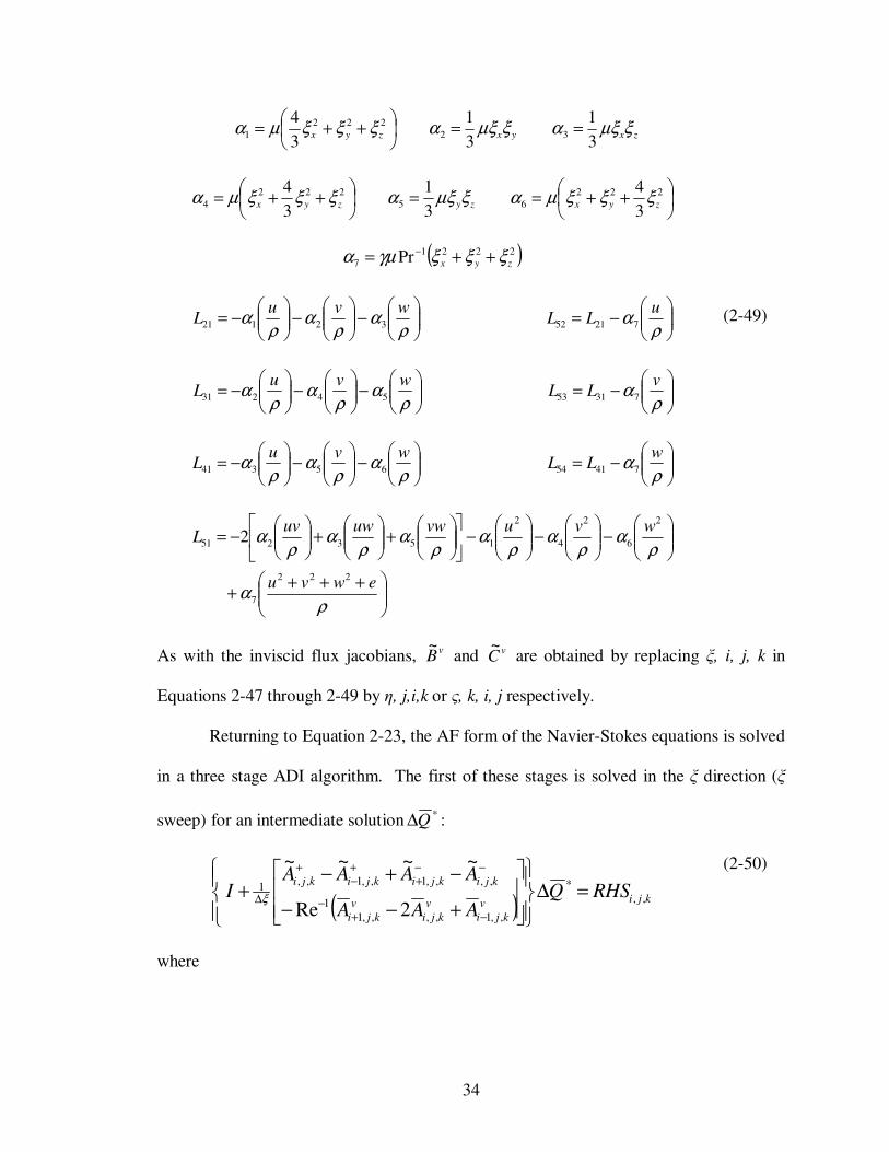
34
zxyxzyx ξµξαξµξαξξξµα3
1
3
1
3
432
222
1 ==
++=
++==
++= 222
65
222
43
4
3
1
3
4zyxzyzyx ξξξµαξµξαξξξµα
( )2221
7 Pr zyx ξξξγµα ++= −
−
−
−=
ρα
ρα
ρα
wvuL 32121
−=
ρα
uLL 72152
−
−
−=
ρα
ρα
ρα
wvuL 54231
−=
ρα
vLL 73153
−
−
−=
ρα
ρα
ρα
wvuL 65341
−=
ρα
wLL 74154
++++
−
−
−
+
+
−=
ρα
ρα
ρα
ρα
ρα
ρα
ρα
ewvu
wvuvwuwuvL
222
7
2
6
2
4
2
153251 2
(2-49)
As with the inviscid flux jacobians, v
B~
and vC~
are obtained by replacing ξ, i, j, k in
Equations 2-47 through 2-49 by η, j,i,k or ς, k, i, j respectively.
Returning to Equation 2-23, the AF form of the Navier-Stokes equations is solved
in a three stage ADI algorithm. The first of these stages is solved in the ξ direction (ξ
sweep) for an intermediate solution*
Q∆ :
( ) kjiv
kji
v
kji
v
kji
kjikjikjikjiRHSQ
AAA
AAAAI ,,
*
,,1,,,,1
1
,,,,1,,1,,1
2Re
~~~~
=∆
+−−
−+−+
−+−
−−+
+−
+
∆ξ
(2-50)
where
Page 51
35
( )
( ) ( ) ( )
∂+∂+∂−∂+∂+∂+
+−−=
−
−+
∆∆
nv
nv
nvnnn
nnkn
kji
GFEGFE
QQQRHS
ςςηηξξςηξ
ττ
ˆˆˆReˆˆˆ
~~2
~
1
1
21,1
23'
,,
(2-51)
The second stage is solved in the η direction (η sweep) for a second intermediate solution
**Q∆ :
( )***
,1,,,,1,
1
,,,1,,1,,,1
2Re
~~~~
QQBBB
BBBBI
v
kji
v
kji
v
kji
kjikjikjikji∆=∆
+−−
−+−+
−+−
−−+
+−
+
∆η
(2-52)
Finally, the third stage is solved in the ς direction (ς sweep):
( )**
1,,,,1,,
1
,,1,,1,,,,1~
2Re
~~~~
QQCCC
CCCCI
v
kji
v
kji
v
kji
kjikjikjikji∆=∆
+−−
−+−+
−+−
−−+
+−
+
∆ς
(2-53)
where the desired solution 1,1~ ++ knQ is obtained via:
( ) QQQQQQ knknknkn ~~~~~~ ,11,1,11,1 ∆+=⇒−=∆ ++++++
(2-54)
Equations 2-50 through 2-53 form a block tridiagonal coefficient matrix system, which is
symmetric positive definite. To obtain this form, Equations 2-50 through 2-53 are first
rearranged in terms of the grid index:
( )[ ] ( )[ ]( )[ ]
kjikji
v
kjikji
kji
v
kjikjikjikji
v
kjikji
RHSQAA
QAAAIQAA
,,
*
,,1,,1
1
,,11
*
,,,,
1
,,,,1*
,,1,,1
1
,,11
Re~
Re2~~
Re~
=∆−+
∆+−++∆+−
++−−
+∆
−−+∆−−
−+−∆
ξ
ξξ
( )[ ] ( )[ ]( )[ ] *
,,
**
,1,,1,
1
,1,1
**
,,,,
1
,,,,1**
,1,,1,
1
,1,1
Re~
Re2~~
Re~
kjikji
v
kjikji
kji
v
kjikjikjikji
v
kjikji
QQBB
QBBBIQBB
∆=∆−+
∆+−++∆+−
++−−
+∆
−−+∆−−
−+−∆
η
ηη
( )[ ] ( )[ ]( )[ ] **
,,11,,1,,
1
1,,1
,,,,
1
,,,,1
1,,1,,
1
1,,1
~Re
~
~Re2
~~~Re
~
kjikji
v
kjikji
kji
v
kjikjikjikji
v
kjikji
QQCC
QCCCIQCC
+++−−
+∆
−−+∆−−
−+−∆
∆=∆−+
∆+−++∆+−
ς
ςς
(2-55)
(2-56)
(2-57)
Page 52
36
Redefining the terms in Equations 2-55 through 2-57 as:
( )( )
( )v
kjikji
v
kjikjikji
v
kjikji
AACAP
AAAICA
AACAM
,,1
1
,,11
,,
1
,,,,1
,,1
1
,,11
Re~
Re2~~
Re~
+−−
+∆
−−+∆
−−+
−∆
−=
+−+=
+−=
ξ
ξ
ξ
( )( )
( )v
kjikji
v
kjikjikji
v
kjikji
BBCBP
BBBICB
BBCBM
,1,
1
,1,1
,,
1
,,,,1
,1,
1
,1,1
Re~
Re2~~
Re~
+−−
+∆
−−+∆
−−+
−∆
−=
+−+=
+−=
η
η
η
( )( )
( )v
kjikji
v
kjikjikji
v
kjikji
CCCCP
CCCICC
CCCCM
1,,
1
1,,1
,,
1
,,,,1
1,,
1
1,,1
Re~
Re2~~
Re~
+−−
+∆
−−+∆
−−+
−∆
−=
+−+=
+−=
ς
ς
ς
(2-58)
(2-59)
(2-60)
Equations 2-55 through 2-57 become:
kjikjikjikjikjikjikji RHSQCAPQCAQCAM ,,
*
,,1,,
*
,,,,
*
,,1,, =∆+∆+∆ +−
*
,,
**
,1,,,
**
,,,,
**
,1,,, kjikjikjikjikjikjikji QQCBPQCBQCBM ∆=∆+∆+∆ +−
**
,,11,,,,,,,,1,,,,
~~~kjikjikjikjikjikjikji QQCCPQCCQCCM ++− ∆=∆+∆+∆
(2-61)
(2-62)
(2-63)
Now putting these in a block tridiagonal format, the following is obtained for the ξ
sweep:
=
∆
∆
∆
∆
−−−−−
kjIM
kjIM
kj
kj
kjIM
kjIM
kj
kj
kjIMkjIM
kjIMkjIMkjIM
kjkjkj
kjkj
RHS
RHS
RHS
RHS
Q
Q
Q
Q
CACAM
CAPCACAM
CAPCACAM
CAPCA
,,
,,1
,,2
,,1
*
,,
*
,,1
*
,,2
*
,,1
,,,,
,,1,,1,,1
,,2,,2,,2
,,1,,1
MMOOO
(2-64)
Page 53
37
then for the η sweep:
∆
∆
∆
∆
=
∆
∆
∆
∆
−−−−−
*
,,
*
,1,
*
,2,
*
,1,
**
,,
**
,1,
**
,2,
**
,1,
,,,,
,1,,1,,1,
,2,,2,,2,
,1,,1,
kJMi
kJMi
ki
ki
kJMi
kJMi
ki
ki
kJMikJMi
kJMikJMikJMi
kikiki
kiki
Q
Q
Q
Q
Q
Q
Q
Q
CBCBM
CBPCBCBM
CBPCBCBM
CBPCB
MMOOO
(2-65)
and finally for the ς sweep:
∆
∆
∆
∆
=
∆
∆
∆
∆
−−−−−
**
,,
**
1,,
**
2,,
**
1,,
,,
1,,
2,,
1,,
,,,,
1,,1,,1,,
2,,2,,2,,
1,,1,,
~
~
~
~
KMji
KMji
ji
ji
KMji
KMji
ji
ji
KMjiKMji
KMjiKMjiKMji
jijiji
jiji
Q
Q
Q
Q
Q
Q
Q
Q
CCCCM
CCPCCCCM
CCPCCCCM
CCPCC
MMOOO
(2-66)
In Equations 2-64 through 2-66, IM, JM, KM represent the last i, j, and k index in the
computational grid. For each sweep, the block tridiagonal system is solved using a LU
decomposition method, which is outlined in Appendix A.
Unlike many other CFD models, Corsair is a fully unsteady flow solver and does
not have a steady state capability for multi blade row simulations. This has the
disadvantage of requiring the use of very small initial time steps in order to handle start-
up transients. Solutions are started by ramping up to this small time step and thus wheel
speed over a user specified number of iterations. Once the ramping is complete, the time
step is gradually increased by decreasing the number of iterations per cycle. To facilitate
this tricky procedure, Corsair re-reads the input deck every time a number of pre-
specified iterations have been completed. The number of iterations per cycle is adjusted
according to the residual dumped in the output file after each iteration.
Page 54
38
2.3 Boundary Conditions
One of the most important factors determining the success or failure of a
numerical simulation is the boundary conditions. The boundary conditions used in
Corsair can be broadly classified as either natural boundaries or zonal boundaries [40,41].
Both types of boundaries are handled in a two step method, comprised of an implicit
formulation during pseudo time steps followed by enforcement of the boundary condition
via a post iterative update after each physical time step. The natural boundaries include
the axial inlet and exit along with the hub, outer casing, and airfoil surfaces. Zonal
boundaries comprise the patch and overlay boundaries, including the slip boundary
between adjacent blade rows, the circumferential periodic boundary between adjacent
passages in the same blade row, the Chimera boundary between O-grids and H-grids, and
the continuity condition between the O-grid and clearance grid. A brief description of
each boundary condition is now given along with its numerical implementation in
Corsair.
To apply the implicit portion of the axial inlet boundary condition, the first row of
blocks from equation 2-64 are set as:
0,,1 =kjRHS
ICCA kj ⋅=,,1
IJ
JCCAP
kj
kjkj ⋅
−=
,,1
,,2,,1
(2-68)
Where C is the Courant number (specified in the input deck and allows control of
stability vs. convergence speed), I is the identity matrix, and J is the Jacobian matrix of
coordinate transformation. The post iterative update depends on whether the axial inlet
Page 55
39
flow is subsonic or supersonic. If supersonic, then all flow quantities are set to their free
stream values. If the axial inlet flow is subsonic, however, four quantities are specified
with the fifth being the Riemann invariant. A few different combinations are available
for these four quantities as given in Table 2-2.
BC 1 BC 2 BC 3 BC 4 BC 5
12
12
2
1
−−=
−+=
=
=
=
∞
∞
∞
γ
γ
cuR
cuR
ww
vv
SS
12
12
2
1
−−=
−+=
=
=
=
∞
∞
∞
γ
γ
cuR
cuR
ww
vv
PP tt
( )
12
12
costan
tan
2
1
−−=
−+=
⋅=
⋅=
= ∞
γ
γ
αβ
α
cuR
cuR
uw
uv
SS
( )
12
12
costan
tan
2
1
−−=
−+=
⋅=
⋅=
= ∞
γ
γ
αβ
α
cuR
cuR
uw
uv
PP tt
( )
12
costan
tan
−−=
⋅=
⋅=
=
=
∞
∞
γ
αβ
α
cuR
uw
uv
TT
PP
tt
tt
Table 2-2. List of axial inlet boundary conditions
Where S is entropy; u, v, and w the axial, circumferential, and radial velocities
respectively; R the Riemann invariants; Pt and Tt the total pressure and total temperature;
c the local speed of sound; γ the ratio of specific heats; α and β the flow pitch and yaw
angles respectively; and the subscript ∞ refers to the inlet free stream values.
Similarly, the implicit portion of the axial exit boundary condition involves
setting the last row of blocks from Equation 2-64 as:
0,, =kjIMRHS
ICCA kjIM ⋅=,,
IJ
JCCAM
kjIM
kjIMkjIM ⋅
−= −
,,
,,1,,
(2-69)
As with the axial inlet boundary, the post iterative update depends on whether the axial
exit flow is subsonic or supersonic. If it’s supersonic, then all flow quantities are
Page 56
40
extrapolated from the interior domain. If the axial exit flow is subsonic however, a
constant pressure is imposed at midspan with the pressure at other spans prescribed by
the radial equilibrium condition:
r
v
r
P t
2ρ=
∂
∂
(2-70)
This results in quasi-2d equilibrium flow, where P is the spanwise pressure, vt is the
tangential or axial velocity, and r is the radius from the center of the hub. To obtain the
remaining quantities, the circumferential and radial velocities, along with entropy and the
Riemann invariant are extrapolated from upstream.
For surfaces, including the hub, outer casing, and airfoil, three different types of
boundary conditions exist; slip (Euler condition), no slip with specified heat flux, or no
slip with specified surface temperature. The implicit portion of the slip condition
involves setting the associated RHS and off-diagonal block to zero and the associated
diagonal block to the identity matrix. As an example, consider the hub surface which
becomes a boundary in the zeta sweep:
0**
1,, =∆ jiQ
01,, =jiCC
ICCP ji =1,,
(2-71)
The post iterative update enforces the tangency condition along the surface by setting the
normal contravariant velocity to zero. For reference, the contravariant velocities are
simply those defined in the curvilinear coordinate system and may be written using the
coordinate transformation metrics:
Page 57
41
wvuU zyxt ξξξξ +++=
wvuV zyxt ηηηη +++=
wvuW zyxt ζζζζ +++=
(2-72)
Continuing along with the example of the post iterative update at the hub, the contra-
variant velocity normal to the hub, W, is set to zero and the Cartesian velocities u, v, and
w are solved using:
−
−
−
−−−−
−−−−−
−−−−
=
−
t
t
t
xyyxxyyxxyyx
xzzxyzzxxzzx
zyzyyzzyyzzx
W
V
U
J
w
v
u
ζ
η
ξ
ηξηξζξζξζηζη
ηξηξζξζξζηζη
ξηηξζξζξζηζη
)()()(
)()()(
)()()(1
(2-73)
The pressure and density at the surface are taken to be the same as at the first grid point
above the surface, from which the remaining conservative variables are easily calculated.
As stated earlier, the viscous no slip boundary conditions come in two forms, one
involves specifying a heat flux at the surface while the other requires specifying the
temperature of the surface. The implicit portions of these boundary conditions are very
similar and will be discussed together. To begin, the RHS block of the associated
boundary is set to zero and the associated diagonal block is defined as:
( )
⋅−⋅−⋅−++⋅ CwCvCuCwvuC
C
C
C
wallwallwallwallwallwall
222
0000
0000
0000
0000α
(2-74)
Where C is the courant number and uwall, vwall, and wwall are the velocities at the surface in
Cartesian coordinates. For a specified temperature at the surface, α is simply set to the
courant number, while for a specified heat flux at the surface it is defined as:
Page 58
42
))/(1(* kTTC wall ⋅∂+=α (2-75)
Where ∂T is the specified heat flux at the surface, Twall is the surface temperature, and k is
the thermal conductivity of the flow over the surface. The associate off diagonal block is
defined as:
( )
−−−++
+
1
00000
00000
00000
222
54321
1
wallwallwallwallwallwall
wall
wall
wvuwvu
JJ
βββββ
(2-76)
For the case of a specified heat flux, β1 = 1 and β2 = β3 = β4 = β5 =0. If the temperature at
the surface is specified instead:
)/(1
)/(
)/(
)/(
)/()(
5
14
13
12
2
1
2
1
2
121
1
wallv
wallvwall
wallvwall
wallvwall
wallvwallwallwall
Tc
Tcw
Tcv
Tcu
Tcwvu
=
=
=
=
++=
+
+
+
+++
β
β
β
β
β
(2-77)
Where the subscript wall+1 denotes values at the grid point just above the surface, cv is
the specific heat at constant volume, and Twall is the specified temperature of the surface.
The post iterative update involves calculating density at the surface based on the
temperature at the surface:
wall
wallwall
TR
P
⋅= +1ρ
(2-78)
Page 59
43
The pressure at the surface is taken to be the same as the grid point just above the surface,
thus allowing total energy at the surface to be easily calculated. For the case where heat
flux at the surface is specified, the temperature at the wall is approximated as:
( )kTdsTT wallwall /1 ∂⋅+= +
(2-79)
Where ds is the distance between the surface and the first grid point above the surface.
The slip boundary between adjacent blade rows begins with the generation of the
H-grids for the blade rows themselves. When initially generated, the downstream
boundary of the upstream row grid corresponds to the upstream boundary of the
downstream row grid. The upstream row grid is then extended downstream by two axial
grid locations such that they match the first two upstream axial grid locations from the
downstream row grid. Finally, the downstream row grid is extended upstream by two
axial grid locations in the same fashion. This process is illustrated for a 2D radial slice in
Figure 2-2.
Page 60
44
Initially generated
downstream H-grid
Downstream extension added
to upstream H-grid
Upstream extension added
to downstream H-grid
Initially generated
upstream H-grid
Common axial location Axial
Cir
cum
fere
nti
al
Figure 2-2. Generation of grid extensions for slip boundary condition
Post iterative update to upstream boundary of
downstream H-grid from upstream H-grid
Post iterative update to downstream boundary of
upstream H-grid from downstream H-grid Axial
Cir
cum
fere
nti
al
Figure 2-3. Post iterative update for slip boundary condition
Page 61
45
The implicit portion of the slip boundary is applied as a dirichlet condition by setting the
associated RHS and off diagonal blocks to zero and the diagonal block to the identity
matrix. The post iterative update consists of setting values on the boundary to those of
the associated overlap grid locations as illustrated in Figure 2-3. The reason for
extending the grid overlap between adjacent blade rows by two grid locations rather than
by a single location is to ensure the boundary conditions do not interfere with one another
and produce spurious numerical oscillations. When the number of circumferential
locations is different between the upstream and downstream H-grids (as shown in the
illustrations), simple linear interpolation is used to obtain the value from the closest two
circumferential grid locations. This same linear interpolation with simple periodicity is
also used for cases when blade rows are rotating relative to one other. For such cases, the
circumferential and radial Cartesian velocities are first transformed into tangential and
normal velocities which are used for the interpolation, after which the circumferential and
radial Cartesian velocities are recovered based on the circumferential angle of the point
being interpolated.
The circumferential periodic boundary condition between adjacent passages in the
same blade row employs an integrated implicit portion. This results in no modification of
the RHS or coefficient matrix blocks. Instead, all values calculated on the boundary use
quantities from ghost points created by the periodic condition, including the metrics of
coordinate transformation. Figure 2-4 illustrates the periodic condition along with the
ghost points for a 2D radial slice. In Figure 2-4, dashed lines show the cells formed by
the ghost points and the arrows indicate where values for the ghost points are taken from.
Page 62
46
Similarly, the post iterative update is based on the periodic condition as well, but is
enforced at the boundary instead of the ghost points, as illustrated in Figure 2-5.
Axial
Cir
cum
fere
nti
al
Figure 2-4. Illustration of circumferential periodic condition and ghost points
Axial
Cir
cum
fere
nti
al
Figure 2-5. Post iterative update of circumferential periodic boundary
Page 63
47
The Chimera patch boundary condition between an O-grid and H-grid on which it
is overlaid, uses a dirichlet condition for the implicit portion. This is similar to what is
done for the axial slip boundary, except in addition to points on the boundary, points cut
from the interior of the H-grid to accommodate the O-grid are also “zeroed out” by
setting their associated RHS and off diagonal blocks to zero along with their diagonal
block to the identity matrix. To apply the post iterative update, values at the boundary
are interpolated from the overlapping grid using shape functions. The shape functions are
not only used for weighting the surrounding values for the interpolation, but also serve to
determine if a point being interpolated lies in the triangle formed by three points from the
overlapping grid. As an example, take the small section of the overlap between an H-grid
and O-grid for a 2D radial slice as illustrated in Figure 2-6.
P
1 2
3 4
Figure 2-6. Section of overlap region between an O-grid and H-grid
In Figure 2-6, point P is on the boundary of the O-grid and for the post iteration update
the conservative variables at point P are interpolated from the portion of the H-grid which
encloses it, namely points 1 – 4. Figure 2-7 is a simplified illustration of this and
Page 64
48
includes the location of the shape functions (N1-N6) which will be calculated, first to
determine which triangular half encloses point P and second to interpolate the values at
point P by weighting the contribution from each of the points in the triangular half
determined to enclosed point P. The reason for splitting the box which encloses point P
into two triangles is because the shape functions for a triangle can be calculated using
global coordinates. By contrast, the shape functions for a box require the use of local
coordinates based about the centroid of the box.
P
1 2
3 4 N4
N5
N6
N3
N2 N1
Figure 2-7. Simplified view of overlap region between O-grid and H-grid
The shape functions for the case illustrated in Figure 2-7 are as follows:
( ) ( ) ( )[ ]
( ) ( ) ( )[ ]
( ) ( ) ( )[ ]
( ) ( ) ( )[ ]
( ) ( ) ( )[ ]
( ) ( ) ( )[ ]
( )
( )
+=
−−−++=
−−−++=
−+−+−=
−+−+−=
−+−+−=
−+−+−=
−+−+−=
−+−+−=
−
zy
zyyz
yzxyzxyzxyzxyzxyzxA
yzxyzxyzxyzxyzxyzxA
yzxxxyzyzyzxyzxA
N
yzxxxyzyzyzxyzxA
N
yzxxxyzyzyzxyzxA
N
yzxxxyzyzyzxyzxA
N
yzxxxyzyzyzxyzxA
N
yzxxxyzyzyzxyzxA
N
pp
pp
pp
pp
pp
pp
122
3423422443322
2312311332211
23322332
2
6
42244224
2
5
34433443
2
4
12211221
1
3
41144114
1
2
24422442
1
1
tan
2
1
2
1
2
1
2
1
2
1
2
1
2
1
2
1
(2-80)
Page 65
49
Where A1 and A2 are the areas of the two triangles formed by points 1 2 4 and 2 3 4
respectively, and yz is the equivalent arc length at a fixed radius. All three shape
functions for the triangle which contains point P will have a value between 1 and 0. If
the triangle doesn’t enclose point P, at least one of the shape functions will have a value
outside this range. In Corsair, a simple brute force search is used to determine the
triangle to use for interpolating the values at each of the boundary points. However, the
shape functions give more information than just whether a point lies in or outside the
triangle formed by them, it also indicates which direction point P lies if it’s outside the
triangle. This idea is elaborated in Appendix B and used to speed up the search of
interpolation points, particularly when the O-grid and H-grid are moving relative to one
another. Given the three shape functions for the triangle in which point P lies (N1 N2 N3
in this case), the values at point P are interpolated via:
442211 ϕϕϕϕ ⋅+⋅+⋅= NNNp
(2-81)
Where φ represents the five conservative flow variables and the subscripts denote the
point location of the variable.
When a clearance grid is used, boundary conditions are not only needed to
enforce continuity between the O-grid and clearance grid but also at the collapsed
centerline of the clearance grid. Both of these conditions arise in the eta sweep of the
clearance grid, with no modifications required to the solution of the O-grid. These
boundary conditions begin with the generation of the clearance grid, which is extended
by one constant eta “ring” such that the outer two rings of the clearance grid coincide
with the two inner most rings of the O-grid. Figure 2-8 illustrates this overlap of the
constant eta “rings” between the O-grid and clearance grid.
Page 66
50
Figure 2-8. Illustration of overlap between an O-grid and clearance grid
The implicit portion of these boundary conditions involves using 10 ghost points in the
eta direction from the O-grid to extend the calculation of the clearance grid well into the
O-grid region. The primary reason for this is stability, since the number of constant eta
“rings” is often very small, especially for thin airfoils. Next the RHS and off diagonal
blocks for the first and last locations (i.e. j=1 and j=JM+10) are set to zero while the
associated diagonal block for these two locations is set to the identity matrix. After
solving the block tri-diagonal matrix, only values for the original clearance grid are
updated. Due to the eta extension into the O-grid, no post iterative update is needed at
the O-grid clearance grid interface. However, a post iterative update is required at the
collapsing centerline of the clearance grid to maintain continuity of the flow. This post
iterative update involves interpolating values at the collapsed centerline from the opposite
Page 67
51
j=2 constant eta “ring”, as illustrated in Figure 2-9. The interpolation is a simple linear
one based on axial locations.
j=2 “ring”
j=1 collapsed
centerline
j=2 “ring”
Interpolate using these two
values to axial location of
opposite j=1 point.
Axial direction
Figure 2-9. Post iterative update of clearance grid collapsing centerline
In this chapter, a detailed discussion of the solution method employed by Corsair
has been covered. An overset O-H grid topology based on curvilinear coordinates is used
upon which to solve the equations of motion on. The equations of motion are derived
from the three dimensional Navier-Stokes equations with a dual (or pseudo) time step to
improve convergence. After non-dimensionalization, the three dimensionally coupled
equations of motion are split into three one dimensional equations using an Approximate
Factorization. This results in a set of one dimensional equations with an explicit RHS
and an implicit LHS, which are then solved in succession along each curvilinear
coordinate using an Alternating Diagonal Implicit algorithm. In addition, a brief
discussion of the boundary conditions available in Corsair was given.
Page 68
52
3. NUMERICAL EVALUATION OF
COORDINATE TRANSFORMATION METRICS
As covered in the previous chapter, Corsair uses a body-fitted curvilinear
coordinate system to help generalize the equations of motion. To convert between these
curvilinear coordinates and actual spatial coordinates, a mapping in the form of
coordinate transformation metrics is used. While mathematical formula for these metrics
was given in the previous chapter, the actual numerical evaluation of these
transformations is a bit different and, as will be shown, more than one method for their
evaluation exists in the open literature. Additionally, the numerical evaluation of the
temporal metrics in the version of Corsair distributed by NASA is incomplete; it is based
on an assumption of only rigid fluid grid rotation about the axial centerline. The
deforming fluid grids ultimately arising from the FSI module require a complete
implementation of the temporal metrics. Thus, this chapter explores several methods in
the open literature for the numerical evaluation of both spatial and temporal metrics,
including comparisons of their performance when implemented in Corsair, with the best
method being used for the remainder of this research.
The use of higher order finite difference schemes to solve non-trivial 3D
geometries demands that issues of free-stream preservation and metric cancellation be
carefully addressed. Such errors, which arise in the finite difference discretization of the
governing equations when written in the conservative form, can catastrophically degrade
Page 69
53
the fidelity of second and higher order approaches [42,43]. By deriving the equations of
motion in conservative form, the following identities have been implicitly invoked:
( ) ( ) ( ) 0///1 =++= ζηξ ζηξ JJJI xxx
( ) ( ) ( ) 0///2 =++=ζηξ
ζηξ JJJI yyy
( ) ( ) ( ) 0///1 =++= ζηξ ζηξ JJJI zzz
( ) ( ) ( ) ( ) 0////14 =+++= ζηξτ ζηξ JJJJI ttt
(3-1)
(3-2)
(3-3)
(3-4)
The first three identities constitute a differential statement of surface conservation for a
closed cell, while the fourth identity expresses volume conservation and is often referred
to in the literature as the Geometric Conservation Law (GCL). While the definitions for
the coordinate transformation metrics given in Equation 2-18 were sufficient to derive the
equations of motions for body fitted curvilinear coordinates, they fail to satisfy these
metric identities due to the lack of metric cancellation, resulting in grid induced errors for
regions of large variation and near singularities. Two main methods have been
introduced in the CFD community for enforcing these metric identities for higher order
finite difference schemes.
3.1 Recasting in Conservative Form
Thomas and Lombard [44] proposed recasting the coordinate transformation
metric equations in a “conservative” form prior to discretization:
Page 70
54
[ ] [ ] [ ]ηζζηηζζηηζζη ξξξ )()()()()()( yxyxJxzxzJzyzyJ zyx −=−=−=
[ ] [ ] [ ]ζξξζζξξζζξξζ ηηη )()()()()()( yxyxJxzxzJzyzyJ zyx −=−=−=
[ ] [ ] [ ]ξηηξξηηξξηηξ ζζζ )()()()()()( yxyxJxzxzJzyzyJ zyx −=−=−=
(3-5)
When the transformation metrics are recast in this manner and the derivatives are
evaluated with the same high-order formulas employed for the fluxes, free-stream
preservation is recovered in general time-invariant 3D curvilinear geometries [45].
For deforming and moving grids, identity I4 must also be satisfied to eliminate
metric cancellation errors and to ensure free-stream preservation. As distributed, Corsair
does not take this into account since the only rigid grid motion around the axial centerline
of the geometry is used and thus there is no grid deformation. However, since the FSI
module being linked to Corsair will introduce both grid deformation and grid motion
other than around the axial centerline, the physical time step derivative in Equation 2-16
is split using the chain rule of differentiation as follows:
( ) ( ) ( )ττττ JQQJJQQ 11~
⋅+⋅==
(3-6)
The reason for applying this only to the physical time step is that all grid point locations
are held fixed during the pseudo time step. To incorporate this modification into Corsair,
the time derivative of the inverse Jacobian is calculated at the beginning of each physical
time step and simply combined with the RHS. Instead of attempting to compute the time
derivative of the inverse Jacobian directly from the grid coordinates at various time levels
(either analytically or numerically), the GCL identity I4 is invoked to evaluate ( )τJ1 :
Page 71
55
( ) ( ) ( ) ( )[ ]ζηξτ ζηξ JJJJ ttt ++=1
(3-7)
Where the time metrics are defined as:
( ) ( ) ( )[ ]
( ) ( ) ( )[ ]
( ) ( ) ( )[ ]JzJyJxJ
JzJyJxJ
JzJyJxJ
zyxt
zyxt
zyxt
////
////
////
ζζζζ
ηηηη
ξξξξ
τττ
τττ
τττ
++−=
++−=
++−=
(3-8)
In many practical applications involving deforming grids (such as the dynamic
aeroelastic FSI model developed), the grid speeds are not known a priori and must
therefore be approximated to the desired degree of accuracy using the evolving
coordinates at several time levels. Higher order finite difference schemes retain their
superior accuracy on rapidly distorting grids when this procedure is used to determine the
time metrics [46].
3.2 Finite Volume Concept
An alternate approach to enforcing the metric identities and thus preserving free-
stream capturing in high order finite difference schemes is the finite volume to finite
difference concept proposed by Vinokur [47]. In this approach, the coordinate
transformation metrics represent normal surfaces and the Jacobian becomes the inverse of
the volume formed by these surfaces. This approach begins with the derivation of the
finite volume formulation, which is then adapted to the finite difference grid. The
integral form of the metric identities can be written as:
∫ =S
dSn 0 (3-9)
Page 72
56
dtdSvntVtV c
t
ttS
⋅=− ∫ ∫2
1
)(12 )()(
(3-10)
where S represents the cell surface, n is the normal to the surface, V is the volume of the
cell, and vc represents the surface velocity relative to the non-inertial frame but expressed
in the inertial frame. The first identity is a mathematical expression for a closed cell
while the second identity represents the conservation of volume for a time-varying cell
from time t1 to time t2. By applying the same curvilinear coordinate transformation as
used with the governing equation of motion, these two expressions take the following
differential form for a finite volume:
( ) ( ) ( )
( ) ( ) ( )ζτζ
ητη
ξτξ
τ
ζζ
ηη
ξξ
rSrSrSV
SSS
⋅+⋅+⋅=
=++ 0
(3-11)
(3-12)
Where the surfaces and volume are related to the metric derivatives and Jacobian by:
[ ]
[ ]
[ ]
[ ]
JrrrV
JrrS
JrrS
JrrS
zyxr
T
zyx
T
zyx
T
zyx
T
1
1
1
1
=×⋅=
=×=
=×=
=×=
=
ζηξ
ηξζ
ξζη
ζηξ
ζζζ
ηηη
ξξξ
(3-13)
Figure 3-1 shows a regular hexahedral cell for a finite volume, where all the edges are
assumed to be straight lines.
Page 73
57
ξ
η ζ
Sξ
1
5
6 7
8
4
2 3
Figure 3-1. Geometry of a finite volume hexahedral cell
From Figure 3-1, the surface vectors are given by:
( ) ( )
( ) ( )
( ) ( )421321
184521
251621
rrrrS
rrrrS
rrrrS
−×−=
−×−=
−×−=
ζ
η
ξ
(3-14)
Note that the surface vectors are taken in the positive coordinate direction so as to satisfy
the geometric identities on the hexahedron. The surface vector evaluations in Equation 3-
14 can be regarded as the evaluation of the free-stream capturing metrics for a stationary
grid.
Next the standard time metrics are considered using finite volume notation:
τζ
τη
τξ
ζ
η
ξ
rSJ
rSJ
rSJ
t
t
t
⋅−=
⋅−=
⋅−=
(3-15)
Page 74
58
Unfortunately, it has been shown that time metrics in equation 3-15 will not maintain the
free-stream even with the use of free-stream capturing metrics [48]. Even worse, such
inconsistent time metrics do not satisfy the GCL. To demonstrate this, consider Equation
3-12, which represents the GCL in finite volume. Now let the grid move in the rigid
rotation, that is Vτ = 0 and rτ = U x r. Then the left hand side of Equation 3-12 is zero,
but the right hand side results in ( ) ( ) ( ) 0≠×+×+× ζζ
ηη
ξξ SrSrSr . This indicates that
the use of the GCL condition (Equation 3-12) for computing Vτ can be erroneous. In
other words, the GCL condition is necessary to preserve the free-stream, but not
sufficient to construct consistent metrics in space and time. Fortunately, this can be
overcome by redefining the time metrics as the time averaged volume swept by the
surface [47]:
t
VdtrS
tJ
t
VdtrS
tJ
t
VdtrS
tJ
St
t
t
St
t
t
St
t
t
∆−=⋅
∆−=
∆−=⋅
∆−=
∆−=⋅
∆−=
∫
∫
∫
ζ
η
ξ
τζ
τη
τξ
ζ
η
ξ
2
1
2
1
2
1
1
1
1
(3-16)
To demonstrate this, let S(t1) = S1562 and S(t2) = S1’5’6’2’ as illustrated in Figure 3-2. The
volume swept by the xi surface vector between time t1 and time t2 becomes:
( ) ( )1'61562'1'1225'5'1131
'5'566'1'122 rrSSSVVS
−⋅++==ξ (3-17)
Page 75
59
1
2
6
5 2’
1’
5’
6’
S(t1)
S(t2)
Figure 3-2. Volume swept by a surface
It is worth noting that the time metrics defined by Equation 3-16 contain all information
about the movement of a cell surface, including translation, rotation, and deformation.
By contrast, the time metrics in Equation 3-15 are a simple product of the surface area
and velocity of the cell centroid, thus they can only represent translational motion. As
with the previous discussion of the Thomas and Lombard approach, the physical time
step derivative in Equation 2-16 is split using the chain rule of differentiation as per
Equation 3-6. However, the time derivative of the inverse Jacobian now takes the
following form using the metric identity Equation 3-12 with the modified time metrics
just discussed:
∆+
∆+
∆−==
ζηξ
τ
τ
ζηξ
t
V
t
V
t
VV
J
SSS1
(3-18)
To apply the previous discussion to a finite difference grid, the edges of the
hexahedron in Figure 3-1 are redefined as a double sized cell in the finite difference grid
Page 76
60
(i.e. 1,1,181,1,131,1,121,1,11 ,,,, +−+++−−+−−−− ==== kjikjikjikji rrrrrrrr L ). Since the
surfaces are now effectively quad sized, the surface vectors defined in Equation 3-14
must now be divided by a factor of four and the volume of the cell by a factor of 8. In
order to obtain higher accuracy, the surfaces are evaluated at the center of the hexahedron
as described in reference[48]:
( ) ( )
( ) ( )
( ) ( )kjikjikjikjikji
kjikjikjikjikji
kjikjikjikjikji
rrrrS
rrrrS
rrrrS
,1,1,1,1,1,1,1,181
,,
1,,11,,11,,11,,181
,,
1,1,1,1,1,1,1,1,81
,,
−++−−−++
−−++−++−
−++−−−++
−×−=
−×−=
−×−=
ζ
η
ξ
(3-19)
This helps obtain higher accuracy by relaxing the “straight line edge” requirement for the
hexahedron mentioned earlier, since the line between any three successive points on a
finite difference grid will mostly likely not be straight. For convenience of comparison
with the standard definition, the spatial metric derivatives at point (i, j, k) are evaluated
as:
( )[ ] ( )[ ]( )[ ] ( )[ ]( )[ ] ( )[ ]( )[ ] ( )[ ]( )[ ]
kjikjikjikjikjikji
kjikjikjikjikjikji
kjikjikjikjikjikji
kjikjikjikjikjikji
kjikjikjikjikjikji
kjikjikjikjikjikji
z
yx
zy
xz
yx
zzdzyydyxxdx
zzdzyydyxxdx
zzdzyydyxxdx
zzdzyydyxxdx
zzdzyydyxxdx
zzdzyydyxxdx
dxdydydxJ
dzdxdxdzJdydzdzdyJ
dxdydydxJdzdxdxdzJ
dydzdzdyJdxdydydxJ
dzdxdxdzJdydzdzdyJ
,1,1,1,16,1,1,1,16,1,1,1,16
,1,1,1,15,1,1,1,15,1,1,1,15
1,,11,,141,,11,,141,,11,,14
1,,11,,131,,11,,131,,11,,13
1,1,1,1,21,1,1,1,21,1,1,1,2
1,1,1,1,11,1,1,1,11,1,1,1,1
656581
656581
656581
434381
434381
434381
212181
212181
212181
−++−−++−−++−
−−++−−++−−++
+−−++−−++−−+
−−++−−++−−++
−++−−++−−++−
−−++−−++−−++
−=−=−=
−=−=−=
−=−=−=
−=−=−=
−=−=−=
−=−=−=
−=
−=−=
−=−=
−=−=
−=−=
ζ
ζζ
ηη
ηξ
ξξ
(3-20)
Page 77
61
From Equations 3-13, the volume of the hexahedron cell must be calculated in
order to obtain the Jacobian. While numerous formulas exist for this calculation, the two
most efficient numerical algorithms are the Long Diagonal (LD) method and the Tetrakis
Hexahedron (TH) method [49]. The LD method splits the hexahedron into six tetrahedra,
but introduces directional preferences along the diagonals selected for triangulation,
resulting in a broken symmetry which is undesirable from a physics standpoint. The TH
method preserves the diagonal symmetry by defining an additional vertex at the
barycenter of each face, but as a result requires more floating point operations or flops,
72 compared to 60 for the LD method. The formulas for these methods using the double
sized cell edges are given in Equations 3-21 and 3-22.
( ) ( ) ( )( ) ( ) ( )( ) ( ) ( )1,1,11,1,11,1,11,1,11,1,11,1,1
1,1,11,1,11,1,11,1,11,1,11,1,1
1,1,11,1,11,1,11,1,11,1,11,1,183
−−−+++−−+−+−−−−−++
−−−+++−−−+−+−−++−−
−−−+++−+−+−−−−−++−
−⋅−×−+
−⋅−×−+
−⋅−×−=
kjikjikjikjikjikji
kjikjikjikjikjikji
kjikjikjikjikjikjiLD
rrrrrr
rrrrrr
rrrrrrV
(3-21)
( ) ( )[ ] [ ][ ][ ] ( )[ ( )][ ][ ] [ ]( ) ( )[ ]1,1,11,1,11,1,11,1,1
1,1,11,1,11,1,11,1,1
1,1,11,1,1
1,1,11,1,11,1,11,1,11,1,11,1,1
1,1,11,1,1
1,1,11,1,11,1,11,1,11,1,11,1,1812
−−−−++−−−+++
−−−+−+−−++++
+−−+++
−−−+−+−+−+++−−−++−
−−−−++
−+−+++−−−++−−−++++
−+−⋅
−×−+
−⋅
−+−×−+
−⋅
−×−+−=
kjikjikjikji
kjikjikjikji
kjikji
kjikjikjikjikjikji
kjikji
kjikjikjikjikjikjiTH
rrrr
rrrr
rr
rrrrrr
rr
rrrrrrV
(3-22)
Taking special note of Equation 3-15 with reference to Equation 3-19, the number of
flops for the LD method can be considerably reduced by reusing the calculated surfaces
of the spatial derivatives of the metrics. In addition, the LD and TH methods for
computing the volume of a cell can also be used for calculating the volume swept by each
Page 78
62
surface vector to obtain the time metrics. In comparison with the Thomas and Lombard
approach of recasting the metrics in conservative form, the finite volume concept has the
advantage of not being dependent on the differencing scheme used for the fluxes.
3.3 Performance Investigation
As distributed by NASA, Corsair uses the finite volume concept for the spatial
derivative metrics along with Equation 3-15 for the evaluation of time metrics. However
as shown in reference [48], the resulting time metrics are then inconsistent. In addition,
since grids are not allowed to deform in the version of Corsair distributed by NASA, the
time derivative of the Jacobian is not included in the time derivative of the solution
vector Q.
An investigation of the two methods just discussed for evaluating both the spatial
and temporal metrics was performed using the procedure in reference [50], the results of
which were then used to determine the best method to implement in Corsair to correct the
metric calculation deficiencies. For these test, all boundary conditions were turned off
and Corsair was compiled with double precision (15 digits) floating point accuracy. To
ensure all boundary conditions had been turned off, an uniform flow field (u=1, v=w=0)
was marched in time on a 21x21x21 uniform grid with unity spacing between adjacent
points (which effectively sets the metrics to unity) for 200 time steps with a ∆t of 0.05.
As expected, there was no variation in the v and w velocities from their initial values of
zero. The procedure in reference [50] involves reproducing this same free-stream flow,
but on a heavily distorted or wavy 3D grid. Error is measured as maximum variation in
Page 79
63
the v and w velocities from zero. The wavy 3D grid used for these tests is defined by the
following formulae:
( ) ( ) ( )
1;
1;
1;1;1;1
)1(sin
)1(sin)2sin()1()(
)1(sin
)1(sin)2sin()1()(
)1(sin
)1(sin2sin1
000
000min,,
00
0min,,
00
0min,,
−=∆
−=∆
−=∆===
∆−
∆−+−∆+=
∆−
∆−+−∆+=
∆−
∆−+−∆+=
KL
Lz
JL
Ly
IL
LxKLkJLjILi
L
yjn
L
xinAkzzz
L
zkn
L
xinAjyyy
L
zkn
L
yjnAixxx
zyx
y
zy
x
zxzkji
z
yz
x
yx
ykji
z
xz
y
xy
xkji
KKK
πππωττ
πππωττ
πππωττ
(3-23)
To begin with, a stationary 3D wavy grid as shown in Figure 3-3 was generated from
Equation 3-23 by setting the parameters IL=JL=KL=21, Ax=Ay=Az=1, Lx=Ly=Lz=4,
nxy=nyz=…=nzy=4, ω=1, and τ=0.25 (the time at which maximum displacement occurs).
Figure 3-3. Three-dimension wavy grid
Page 80
64
This grid was then used to evaluate the performance of the spatial derivative metrics. An
initial solution of uniform flow (u=1, v=w=0) was then marched in time for 50 time steps
with a ∆τ=0.05 using first, second, and third order spatial accuracy with three Newton
sub-iterations. The resulting maximum deviations of the v and w velocities from zero for
the various methods and spatial accuracy are displayed in Table 3-1.
1st Order 2
nd Order 3
rd Order
Standard Definition 7.271E-2 1.011E-1 1.162E-1
Conservative Recasting 7.463E-14 1.085E-14 1.140E-14
FV Concept w/ LD 5.859E-16 6.320E-16 6.358E-16
FV Concept w/ TH 5.122E-16 6.154E-16 5.215E-16
Table 3-1. Free-stream preservation errors for stationary 3D wavy grid
As expected, the largest error occurs for the standard definition of the metrics given in
Equation 2-18. While the conservatively recast metrics of Thomas and Lombard show
significant improvement compared to the standard definition, they are not quite as
accurate as the finite volume concept. This may be due to the accumulation of numerical
or round off error, as the conservative recasting method does entail significantly more
numerical operations than the finite volume concept. There is little to no difference
between the long diagonal (LD) and tetrakis hexahedron (TH) methods used to calculated
volumes in the finite volume concept method. However, the long diagonal does have the
advantage of requiring significantly fewer flops since the surface vectors can be reused in
calculating the volume of the cell.
Page 81
65
Next, the ability of each method to preserve the free-stream on a dynamically
deforming curvilinear grid was tested. Again, the wavy 3D grid described by Equation 3-
23 was used but with the following parameters: IL=JL=KL=31, Ax=Ay=Az=1.5,
Lx=Ly=Lz=12, nxy=nyz=…=nzy=4, and ω=1. An initial uniform flow solution was
marched in time with a ∆τ=0.005 for 50 time steps with the grid deformed at each time
step according to Equation 3-23. Thus, the 3D grid begins with a uniform spacing of 0.4
between adjacent points but ends up with the maximum deformation similar to Figure 3-3
after 50 time steps. As with testing of the spatial metric derivatives, this simulation was
run for first, second, and third order spatial accuracy with different combinations of
temporal and spatial metric derivative calculation methods. The resulting maximum
deviation of v and w from their initial value of zero for each combination is shown in
Table 3-2 and is used to gauge their performance.
Spatial Method Temporal Method 1st Order 2
nd Order 3
rd Order
Corsair (No Jτ Correction)
FV Concept (LD) & Std. Def.
6.865E-2 8.552E-2 8.813E-2
Std. Def. Std. Def. 4.396E-3 4.783E-3 4.718E-3
Std. Def. VS(LD) 3.945E-3 4.541E-3 4.489E-3
Conserv. Recast Std. Def. 6.506E-8 3.944E-13 2.613E-13
Conserv. Recast VS(LD) 2.321E-9 1.283E-13 1.022E-13
FV Concept (LD) Std. Def. 6.020E-9 1.461E-14 2.613E-14
FV Concept (LD) VS(LD) 7.052E-11 2.928E-15 1.385E-16
FV Concept (TH) VS(TH) 5.625E-11 2.344E-15 1.254E-16
Table 3-2. Free-stream preservation errors for deforming 3D wavy grid
In Table 3-2, the first method tested is the unmodified version of Corsair in which the
Jacobian is assumed not to change with time. The remainder of Table 3-2 is split up into
Page 82
66
combinations of methods for evaluating the spatial and temporal metric derivatives. For
spatial methods, Std. Def. is the standard definition given by Equation 2-18, Conserv.
Recast is the conservatively recast form of the spatial metrics given by Equation 3-5, and
FV Concept (LD) & FV Concept (TH) are the finite volume concept given in Equation
3-19 with the volume of the hexahedron calculated using the long diagonal and tetrakis
hexahedron methods, respectively. For the temporal methods, Std. Def. is the standard
definition given in Equation 3-8, and VS(LD) & VS(TH) are the finite volume concept of
a volume swept by the surface vectors given in Equation 3-16 using the Long Diagonal
and Tetrakis Hexahedron formulae respectively.
Results for the unmodified version of Corsair illustrate the importance of
including the temporal derivative of the Jacobian in the temporal derivative of the
solution vector Q, even with a high order spatial metric derivative method. Along similar
lines, the results using the standard definition for the spatial metric derivatives show large
errors, regardless of the spatial metric derivative method used. The conservative
recasting method for the spatial metric derivatives shows marked improvement over the
standard definition, but still has a larger error than the finite volume concept method. A
slight improvement gain for the conservative recasting method is shown when paired
with the swept volume idea from the finite volume concept method for calculating the
temporal metric derivatives. Most likely, this improvement is the result of accounting for
deformation of the spatial metrics between time steps. When paired with the standard
definition for the temporal metric derivatives, the finite volume concept using long
diagonals results in error similar to that for the conservatively recast metrics method.
However, when the finite volume method for spatial metric derivatives is paired with the
Page 83
67
swept volume method for the temporal metric derivatives, the error is noticeably reduced.
Lastly, there appears to be very little difference in terms of error between using the long
diagonal or tetrakis hexahedron methods for calculating volumes when the finite volume
concept is used for both spatial and temporal metric derivatives.
In this chapter, three numerical methods for the evaluation of the coordinate
transformation metrics were investigated for use in Corsair. These methods included the
standard analytical form, the conservatively recast form, and the finite volume to finite
difference concept. Each method was examined using a highly distorted static and
dynamically deforming, wavy grid for spatial and temporal metrics respectively. The
error associated with each method was quantified as the maximum deviation of non-axial
velocities from zero when performing a uniform axial free-stream reproduction test. In
addition, combinations of spatial and temporal methods were compared, including use of
long diagonals and tetrakis hexahedrons for the calculations of volumes in the finite
volume to finite difference method. Results clearly show that the standard analytical
form produces significant free-stream errors when deformed three dimensional grids are
used with a finite difference solver. Hence the standard analytical form of the metrics
should be avoided when using a finite difference solver with a deformed curvilinear grid.
While the conservatively recast method significantly reduced these errors, the finite
volume to finite difference concept was able to reduce them even further and with fewer
floating point operations. Although the tetrakis hexahedron method showed slightly
better results, it requires significantly more floating point operations than the long
diagonal method when reusing the surface vectors (spatial metric derivatives) in
computing the temporal metric derivatives (swept volumes). Thus, the finite volume
Page 84
68
concept with long diagonals was chosen to correct the metric calculation deficiencies in
Corsair.
Page 85
69
4. WALL FUNCTION
As outlined in Section 1.1, one of the main objectives required in order for the
resulting aeroelastic solver to be used as a design tool is reduction of the time required to
run a simulation. One of the most direct ways of achieving this is simply to reduce the
total number of grid points used in the simulation, since the runtime is directly
proportional. In a typical Corsair simulation, the grid density near solid surfaces is
intentionally high in order to accurately calculate the shear stress using a finite difference
approach, a technique commonly known as gridding to the wall. Accurate calculation of
the shear stress is critical, as it is used for calculation of turbulence in the flow and
additionally will be utilized by the FSI module to determine the aerodynamic forces on
the blade surface. By replacing the finite difference calculation of the shear stress with
one based on empirical data (i.e. a wall function), the number of grid points near solid
surfaces and thus the total number of grid points can be substantially reduced while still
obtaining accurate shear stresses. This chapter covers the wall function added to Corsair
for the current research, including the use of the shear stress in the turbulence model, and
a comparison of the two shear stress methods using a fourth standard configuration
turbine blade.
Page 86
70
4.1 Background Boundary Layer Theory
In the 1930s, Prandtl and Von Karman deduced that turbulence consists of three
separate layers: a very small inner layer next to the surface where viscous (molecular)
shear is dominant termed the laminar sub-layer, an outer layer where turbulent (eddy)
shear is dominant called the fully turbulent zone, and a transition layer called the buffer
zone [51]. It is common in turbulence modeling to regroup these three layers into just
two regions, an inner region which includes the laminar sublayer, the buffer layer, and
part of the fully turbulent zone, and an outer region which consists of the remaining part
of the fully turbulent zone [52]. To delineate between these two regions, a non-
dimensional coordinate y+ of approximately 400 is taken to be the upper limit of the inner
region, where y+ is defined as
wall
wallwallyy
µ
τρ=+
(4-1)
Here, y is the normal distance from the wall, ρwall is the density at the wall, τwall is the
shear stress at the wall, and µwall is the laminar viscosity at the wall.
The unsteady Navier-Stokes equations fully describe the fluid flow field including
turbulence, but require resolving very small spatial and temporal details in order to
correctly model turbulence. A common approach used in order to obtain meaningful
results with reasonable grid densities is to average the equations of motion over relatively
small time periods [52]. This results in the Reynolds Averaged Navier-Stokes (RANS)
form of the equations of motion with apparent stresses due to the time unsteadiness.
Boussinesq introduced a hypothesis, commonly referred to as the Boussinesq assumption,
which simply states that the apparent stress can be related to the strain multiplied by the
turbulent viscosity [52]. Thus, to include the effects of turbulence, the molecular
Page 87
71
viscosity µ in the stress terms of the Navier-Stokes Equations is replaced by (µl + µt) and
the term (µ / Pr) in the heat conduction term is replaced by (µl / Prl + µt / Prt), where the l
and t subscripts denote laminar and turbulent quantities respectively. By using this
approach, the Navier-Stokes equations remain unchanged in form. For air, the turbulent
Prandtl number, Prt, and the laminar Prandtl number, Prl, are generally taken to be 0.9
and 0.74 respectively. The laminar viscosity is generally modeled by Sutherland’s law,
where µl is a function of the local static temperature [51]. However, the turbulent
viscosity, µt, is not so easily determined and as a result, several turbulence models have
been developed over the years to solve for this term in order to close the RANS
formulation of the equations of motion.
4.2 Algebraic Model
Zero-equation turbulence models use equations where the turbulent fluctuating
correlations are related to the mean flow field quantities by algebraic relationships. The
underlying assumption in such models is that the local rate of turbulence production is
approximately equal to the rate of turbulence dissipation. Furthermore, they do not
include convection of turbulence. Obviously, this is contrary to the physics of most flow
fields, since the past history of flow must be accounted for. However, these models are
mathematically simple and their incorporation into a numerical code is relatively easy to
accomplish. One of the most commonly used zero-equation turbulence models is the
Baldwin-Lomax model [53]. In this two-layer model, the turbulent viscosity µt is
described by
Page 88
72
>
≤=
−
−
crossoveroutert
crossoverinnert
tss
ss
µ
µµ
(4-2)
Where s is the distance normal to the surface and scrossover is the smallest value at which
µt-inner equals µt-outer. In the inner region, the turbulent viscosity is calculated using the
Prandtl-Van Driest formulation
ωρµ 2lt = (4-3)
where ω is the vorticity defined as
y
u
x
v
∂
∂−
∂
∂=ω
(4-4)
and the mixing length l is given by
−=
− +
+
A
y
eyl 1κ
(4-5)
Here, κ is the Von Karman constant (~0.41) and A+ is a parameter which depends on the
streamwise pressure gradient and has a value of 26 for zero-pressure gradient flows.
However, Granville [54] has provided a review of alternative formulae which may
be used in order to account for the presence of pressure gradients and surface roughness.
He proposed the following formula for the mixing length to most closely match
experimental data
−=
+−++
261
*1
bPy
eyl τκ
(4-6)
where b is set to 14.0 for P+ < 0 (favorable pressure gradient) and to 16.4 for P
+ > 0
(adverse pressure gradient). The parameter P+ represents the pressure gradient and is
defined as
Page 89
73
( ) x
P
uP
wall∂
∂
=+
3*ττρ
ν
(4-7)
Here, ν is the kinematic viscosity and τ* represents the non-dimensional total shear stress
close to the wall and is given by
+++= yP1*τ (4-8)
The turbulent viscosity in the outer region is approximated by
KlebwakeCPtFFCαρµ = (4-9)
where α is the Clauser constant and usually assigned a value of 0.0168 for flows in which
the momentum thickness Reynolds number is greater than 5000, and
( )
∆=
max
2
maxmaxmax ,minG
VyCGyF
wakewake
(4-10)
Typically, Cwake is given a value of 0.25 and the term ymax is the value of y corresponding
to the maximum value of G, denoted Gmax, across the layer where
( )
−==
− +
+
A
y
eyl
yG 1ωωκ
(4-11)
The difference between the absolute values of the maximum and minimum velocities
within the viscous region is denoted by ∆V. For wall bounded flows, the minimum
velocity occurs at the surface where the velocity is zero, thus
( ) 21
222 wvuV ++=∆ (4-12)
For shear layer flows, ∆V is defined as the difference between the maximum velocity and
the velocity at the ymax location, hence
( ) ( ) 21
22221
max
222
maxywvuwvuV ++−++=∆
(4-13)
Page 90
74
FKleb is an intermittency factor which provides additional smoothing and is defined as
16
max
5.51
−
+=
y
yCF Kleb
Kleb
(4-14)
and as before, ymax is the y location where Gmax occurs. Typical values for the Klebanoff
constant CKleb and CCP are 0.3 and 1.6, respectively, for zero to mild pressure gradients.
However, according to Granville [55], these “constants” should really be variable and
suggest a fit to known properties of Cole’s wake law and equilibrium pressure gradients
*1724.0
01312.0
3
2
β−−=
KlebC
(4-15)
where
x
V
u
y
t ∂
∂= max*β
(4-16)
and ut is the friction velocity. The velocity gradient in β* is calculated outside the viscous
region. Once the Klebanoff constant has been evaluated, CCP is calculated using
( )3322
43
KlebKlebKleb
Kleb
CPCCC
CC
+−
−=
(4-17)
This modification is believed to give the Bawin-Lomax model accuracy comparable to
the mixing-length and Clauser iterative models.
Corsair uses the modified version of the Baldwin-Lomax turbulence model just
discussed. Additional modifications, based on the developers’ experience with
compressor and turbine geometries, are also employed in Corsair [56]. First, the
equations are applied along grid lines rather than normals to the surface. This avoids the
calculation of all the normal distances and the interpolation of flow variables. Second,
the switchover location between the inner and outer models is not allowed to move more
Page 91
75
than a specified number of grid points between adjacent streamwise locations. In
addition, a second derivative smoothing function is used on the turbulent viscosity field
in separated flow regions. This eliminates non-physical gradients in the turbulent
viscosity near separation points. Thirdly, a cutoff value is imposed on the turbulent
viscosity (nominally 1200 times the free-stream laminar viscosity). Finally, a limit is
imposed on scrossover in order for it not to occur too far beyond the wall.
4.3 Wall Function Model
Implementation of the Baldwin-Lomax turbulence model requires the wall shear
stress. In the original form of Corsair distributed by the NASA Marshal Space Flight
Center, the wall shear stress is calculated using a finite difference approach. This
requires a very fine grid spacing, or clustering, to be used near solid surfaces such as the
hub, shroud, and blade, in order to resolve the entire boundary layer (y+ ~ 2) and obtain
the correct shear stress. In addition, this fine grid spacing requires a significantly small
time step in order to maintain stability via the CFL law [52]. To overcome these
limitations, wall functions have been implemented in Corsair. Wall functions make use
of empirical data to determine the wall shear stress based on the Reynolds number at a
normalized distance away from the wall. By using this empirical relationship, the grid
needs only to be fine enough near the surface to ensure the log-linear correlation is valid.
According to turbulent boundary layer theory, the inner layer obeys the following
relationship at the wall:
++= uyRe (4-18)
Page 92
76
where y+ is the inner region normalized distance, u
+ is the inner region normalized
velocity, and Re is the local Reynolds number just above the surface. The relationship
between u+ and y
+ is well known from experimental work of turbulent water flow in
smooth pipes [51]. Additionally, Spalding devised a single composite formula which
describes this relationship for the entire wall-related region [57]:
( ) ( )
−−−−+=
+++−++ +
621
32
uuueeuy ub κκ
κκκ (4-19)
In the Equation 4-19, κ is the Von Karman constant and assigned the value of 0.41 while
b is the logarithmic friction law constant and is typically given a value of 5.5 for
hydraulically smooth surfaces. The first part of Equation 4-19 represents the viscous
sublayer (y+ = u
+), while the second half represents the buffer and logarithmic layers.
This formula blends the three regions in a smooth fashion, which shows excellent
agreement with experimental data up to a y+ of ~500, where a slight wake occurs [51].
Implementation of wall functions in Corsair starts with a calculation of the local
Reynolds number at the first grid point away from the surface:
=
l
yW
µ
δρRe
(4-20)
where δy is the normal distance from the surface, W is the relative velocity vector, and ρ
is density. A curve fit to the u+- y
+ relationship from Spalding’s formula along with
Equation 4-1, is then used to determine u+ and y
+ from the calculated local Reynolds
number. Once u+ is known, the shear stress at the wall is given by:
+=
u
Ww
2ρτ
(4-21)
In addition, the local skin friction coefficient can also be calculated according to:
Page 93
77
( )2
2+
=u
C f (4-22)
In terms of the inner law-of-the-wall distance, y+, a maximum value of ~500 can now be
used with wall functions versus a maximum of ~2 without.
4.4 Surface Roughness
Surface roughness (resulting from deposits, erosion, or finishing) can have a
significant effect on the aerodynamic performance of turbomachinery [58,59]. This
effect comes from the break up of the thin viscous sublayer, which increases the wall
friction and thus changes the location of transition from laminar to turbulent flow. Since
surface roughness can greatly change the location of transition, it is important to include
its effect in the turbulence model. The simplest way to incorporate surface roughness in
most turbulence models is through the computation of the wall stress via the wall friction.
In Corsair, such a method described by Shabbir and Turner is utilized [60].
The effect of surface roughness enters Spalding’s formula, Equation 4-19, via the
logarithmic friction law constant b. It is important to note that this limits the effect of
surface roughness to the buffer and logarithmic layers. However, since the lower buffer
layer and laminar sublayer have been blended in Spalding’s formula, the effects of
surface roughness can be applied to the upper part of the buffer layer, at best. Thus, this
limits the minimum y+ for inclusion of surface roughness effects in the wall function
using Spalding’s formula to ~20 [60].
The sand roughness experiments of Nikuradse characterized the effect of
roughness on the velocity profile by the equivalent sand roughness Reynolds number
defined as:
Page 94
78
w
ws
s
kk
µ
ρτρ=+
(4-23)
where ks is the equivalent sand roughness height [61]. The surface is considered
hydraulically smooth if 5≤+sk and is considered completely rough if 70≥+
sk . The
range in between, 705 << +sk , is the known as the transition range. Based on the
measurements of Nikuradse, the logarithmic friction law constant can be expressed as a
function of surface roughness:
( )+−= skBb ln5.2 (4-24)
where the coefficient B has been determined experimentally for a range of surface
roughness values. For hydraulically smooth and rough surfaces, B is a function of +sk ,
but for completely rough surfaces it is a constant with an average value of 8.5.
In the work of Shabbir and Turner, families of curves are plotted for the variation
of the skin friction coefficient as a function of local Reynolds number for various surface
roughness values, where the coefficient B was obtained from reference [61]. This plot is
reproduced here as Figure 4-1 and also includes lines of constant ++ yks . This data was
used to plot the local Reynolds number as a function of the ration between surface
roughness to the first grid point height above the surface ( ++ yks ) for different values of
surface roughness, reproduced here as Figure 4-2. Given these two plots, the local
Reynolds number, and the ratio of surface roughness to the first grid point height above
the surface ( ++ yks ), the skin friction coefficient can be determined explicitly. To aid in
programming this method, the plots in Figures 4-1 and 4-2 have been curve fitted using
polynomials.
Page 95
79
Figure 4-1. Skin friction coefficient as a function of local Reynolds number
Figure 4-2. Local Reynolds number as a function of surface roughness to grid height ratio
Page 96
80
For a given grid and surface roughness, the ratio ykyk ss =++ is fixed. The
corresponding local Reynolds number then determines one of three possible surface
conditions and the associated skin friction. First, a calculation of Resmooth is made from a
curve fit to Figure 4-2 for +sk = 5. If the local Reynolds number is equal to or smaller
than Resmooth then the surface is hydraulically smooth and a curve fit to the skin friction
coefficient is made from Figure 4-1. If the surface is found not to be hydraulically
smooth, then it is checked to see if it is completely rough. To determine this, Rerough is
calculated from the curve fit for +sk = 70 in Figure 4-2. if the local Reynolds number is
equal to or greater than Rerough, then the surface is completely rough and the skin friction
coefficient is computed from a curve fit for +sk = 70 in Figure 4-1.
If the surface is not hydraulically smooth or completely rough, then it is obviously
in the transition region. For this case, the skin friction coefficient is calculated in three
steps. In the first step, ++ yks along with the local Reynolds number Re are used in
conjunction with Figure 4-2 to determine which two lines (out of the seven) encompass
the surface under consideration, call these two associated Reynolds numbers Re1 and Re2.
In the second step, the corresponding lines on Figure 4-1 are identified and the skin
friction coefficients, call them Cf1 and Cf2, are calculated from their curve fits. In the
third step, the desired skin friction coefficient Cf is obtained with a simple linear
interpolation:
( )( )
( )1
12
12
1 ReReReRe
−−
−+= ff
ff
CCCC
(4-25)
Page 97
81
4.5 Test Case
To test the implementation of these wall functions, an appropriate test case is
required. A typical case used to test both the implementation of wall functions and
turbulence models is a flat plate [62,63]. In such test cases, free-stream conditions such
as pressure, temperature, and Mach number are specified and the numerical results
compared to either analytical or experimental data for skin friction at the wall surface. A
major drawback to this particular type of test case involves the difficulty of generating an
O-grid for an infinitely thin flat plate. In addition, the skin friction coefficients used in
the wall function are experimentally obtained from tests on flat plates, making such a test
redundant.
Instead, a more realistic turbomachinery test case involving the fourth standard
configuration (STCF4) is used to test the wall function implementation in Corsair. The
fourth standard configuration represents a typical section of a modern free standing
turbine, with relatively high blade thickness and camber, operating under strong subsonic
flow conditions. It is ideally suited for testing since a wealth of experimental results from
the annular cascade facility at the Lausanne Institute of Technology exists in the public
domain [64]. The cascade consists of twenty prismatic blades, each with a chord of
approximately 2.83 inches and a span of just over 1.57 inches, with 45 degree turning and
a maximum thickness to chord ratio of 0.17. The stagger angle is 56.6 degrees with a
blade to blade pitch of 2.2 inches. For this test, case three of the experimental test series
is used. For this case, the inlet and exit flow angles are 45.5 and 71.0 degrees,
respectively, with inlet and exit Mach number of 0.28 and 0.90, respectively. For this
test, the pressure coefficients at mid-span for both the gridding-to-wall and wall functions
Page 98
82
are compared with experimental measurements. For the gridding-to-wall simulation, a
refined O-grid (271x67x51) with a distance to first grid line from the blade surface of
0.00003 inches was used resulting in a maximum y+ of ~1.85. The wall function
simulation used a coarser O-grid (241x29x51) with a distance to first grid line from the
blade surface of 0.0018 inches resulting in a maximum y+ of ~48.2. For both
simulations, the same H-grid (161x85x51) was used and the simulations were run at third
order accuracy with a single Newton sub-iteration. While three Newton sub-iterations
are generally used to reduce error from the approximate factorization of the governing
equations, a single Newton sub-iteration is sufficient for these runs since the solution is
steady state (not time accurate) and quicker results can be obtained. Both solutions were
run for the same non-dimensional time. However, the gridding-to-wall simulation
required a time step one third the size of the wall function simulation in order to maintain
stability. As a result of the time step and grid size differences, the gridding-to-wall run
took roughly 4.5 times longer than the wall function run. Figure 4-3 is a contour plot of
the Mach numbers for the wall function simulation at mid-span, illustrating the fourth
standard configuration flow domain.
Page 99
83
Figure 4-3. STCF4 flow domain
Figure 4-4 shows the coefficient of pressure at mid-span for the two runs compared with
the time averaged experimental measurements.
Mach Number
0.9
0.8
0.7
0.6
0.5
0.4
0.25
0.15
0.05
Page 100
84
Figure 4-4. STCF4 pressure coefficients at mid-span
As shown in Figure 4-4, there is little to no difference between the results
obtained using the gridding-to-wall method versus the wall function. There is a slight
difference between the two at the trailing edge of the suction side, but this is most likely
due to the vortex shed by the rounded trailing edge of the fourth standard configuration.
Comparison with the experimental data is also quite good. The difference between
experimental and computational simulation results in the first 30% of the chord is due to
uncertainty in the inlet flow angle of the experiment, as described in the Lausanne
Institute of Technology report.
The addition of a wall function to Corsair for the calculation of shear stress at
solid surfaces was discussed in this chapter. A background introduction of boundary
layer theory was presented to show the importance of accurate shear stress calculations
% Chord
Ste
ad
yP
ressu
reC
oe
ffic
ien
t
0 0.2 0.4 0.6 0.8 1
-8
-6
-4
-2
0
Gridding-to-wallWall FunctionExp PSExp SS
Page 101
85
and the use of this quantity in the turbulence model employed in Corsair. The wall
function replaces the gridding-to-the-wall, finite difference approach, used in the original
version of Corsair. Details of the wall function implementation were also covered
including the ability to account for surface roughness. More importantly in meeting the
objectives in section 1.1, the wall function allows for a significant reduction in grid
cluster near solid surfaces, resulting in overall smaller grids and thus reduced runtimes.
Finally, a comparison of the two methods was made using the fourth standard
configuration. The results not only showed a reduction in runtime due to the reduction in
grid size, but also from the ability to use larger time steps while still maintaining stability.
Page 102
86
5. ADDITIONAL PARALLELIZATION
One of the objects for this research as outlined in section 1.1 was to create an
aeroelastic solver that could be used in the design phase of turbomachinery. While the
incorporation of the wall function discussed in the previous chapter significantly reduces
the runtime for a simulation, even greater reductions are desired. This chapter covers the
restructuring/rewriting of the flow solver along with addition domain decomposition
which was added, in order to further reduce runtimes. Details of the computer resources
utilized for this research are also given.
5.1 Existing Parallelization in Corsair
As distributed by NASA Marshall Space Flight Center, Corsair is parallelized for
use with MPI and MP-threads [10]. MPI is used for the coarse breakup of the
computational grid, with each grid being solved on a separate node. MP-threads is used
to further break up the calculations of each grid by using multiple Cores/CPUs on each
node. While the calculations in Corsair have been parallelized via MPI and open-MP, the
data structure has been kept serial. For SMP shared memory architectures such as the
one Corsair was developed on, this program structure is rather efficient. Unfortunately,
this same program structure on distributed memory architectures, such as the Beowulf
cluster used for this research, have severe parallelization and memory limitations. For
example, since the Beowulf cluster used for this research consist of single core nodes, the
Page 103
87
open-MP feature of Corsair could not be used and thus only the coarse breakup of one
grid per node via MPI could be used. Further, the serial data model limits the problem
size that can be solved since the entire problem domain must fit in the memory of each
node used in a parallel run. This serial data model also results in a tremendous amount of
communication, since the entire flow domain must be updated after each iteration on all
nodes used for a parallel run. To overcome these limitations, Corsair was rewritten with
a focus on distributing the data structure with the calculations. The resulting flow solver,
called Thunder, allows for more parallel scalability, a reduced nodal memory footprint,
and the ability to solve larger problem on distributed memory architectures such as the
Beowulf cluster used for this research. In addition, a general clean up of the code is
achieved, resulting in faster performance and allowing for easier integration of the FSI
module.
5.2 Target Computational Platform
For this research, the target computational platform is the Taylor Beowulf cluster
which consists of 92 compute nodes, 3 head nodes, and a file server all connected using a
Gigabit network. The compute nodes are grouped into two racks each composed of 46
nodes and a 48 port gigabit network switch (see Figure 5-1), while a third 48 port gigabit
network switch is used to connect the head nodes and file server together. To tie the
network switches together, two ports from each of the compute node group network
switches are bonded together and connected to the network switch used for the head
nodes and file server in a tree configuration. Although bonding two ports together
effectively doubles the bandwidth between the switches, this does not fully compensate
Page 104
88
for cases where parallel runs are split between compute node racks. However, it was
found during initial setup and testing of the cluster that this tree configuration did provide
better performance than a ring configuration between the three network switches. The
network configuration for the Taylor cluster is shown in Figure 5-2. Each compute node
consists of a single core 2.4 GHz AMD Athlon 64 3800+ processor with 1 GB of
DDR400 RAM along with a 40 GB hard drive providing local scratch space. While
multi-core processors were available, their cost/performance at the time of the Taylor
cluster construction precluded them from being used for the compute nodes. In addition,
the ability for the chosen scheduler & queue system to handle multi-core nodes was not
fully developed yet [65], resulting in the belief that for most users multi-core nodes
would lead to a waste of computing resources. DLink 1248T 48 port GigE switches
along with CaT6 cables are used for the network. The Taylor cluster uses the 64 bit
version of cAos 2.0 Linux distribution along with Torque for the queue system and Maui
for queue management.
Page 105
89
Figure 5-1. Taylor cluster compute node rack
Dlink 1248T
Building LAN
Taylor03 Taylor02 Taylor01
Dlink 1284T
Compute nodes
n001 – n046
1 Gpbs
2 Gpbs
Dlink 1248T
Compute nodes
n047 – n092
Chanute04
File Server
Rack 1 Rack 2
Figure 5-2. Taylor cluster network configuration
Page 106
90
5.3 Code Restructuring
As stated earlier, Corsair uses a parallelized calculation with serial data program
structure. While this type of structure can run efficiently on SMP supercomputers with
shared memory, such a program structure is very inefficient on distributed memory
architectures, such as the Beowulf cluster used in this research, for two primary reasons
[66,37]. First, the serial memory model limits the size of problems which can be solved
to what will fit in the memory of a single node. For the Taylor Beowulf cluster, this
limits the size of a problem to ~1 GB of memory, which based on experience roughly
translates to a problem domain of 1.5 million total grid points when using double
precision accuracy. Second, since each node must maintain an up to date copy of the
entire problem domain (grid points, flow variables, etc.), a tremendous amount of
communication is required between all the nodes after each iteration.
Corsair is written in FORTRAN 77 and thus one of its inconveniences is that the
source code must be recompiled for each new problem size. To do this, a parameter file
containing the index size of several arrays must first be edited to fit the desired target
problem. However, since several key index sizes are grouped together, the resulting
arrays are often much larger than they need to be. Corsair also uses a somewhat unusual
vector based storage method. While large vectors are used to store the solution and grid
points for the entire problem domain, smaller multi-dimensional arrays are used for
temporary storage of appropriate portions of the problem domain while they are being
used in calculations or being solved for. This storage method makes it easier to update
the entire flow domain after each iteration, since the data is already in a packed form, but
Page 107
91
in addition to requiring more memory, it also incurs a heavy time penalty each time a
large portion of these vectors is written into a multi-dimensional array or vice versa.
To overcome these issues, a restructure version of Corsair called Thunder was
developed using only MPI for parallelization. The decision to use MPI instead the mixed
hybrid MPI and openMP model used in Corsair is based on two reasons. First,
programming with hybrid parallel models is prone to errors. Second, modern
implementations of MPI (such as MPICH, LAM, and openMPI) are optimized to run on
multi-core/multi-CPU noded systems just as well as single core/CPU noded systems.
Unlike Corsair, Thunder is written in Fortran 95 and takes advantage of dynamically
allocated multi-dimensional arrays for storing data, thus removing the need to recompile
the code for each new problem size. In addition, each node stores only its portion of the
flow domain, along with a minimum amount of data required for the ghost points. This
significantly reduces the nodal memory footprint, along with the amount of
communication required after each iteration.
Unlike most parallel flow solvers [67], the grid and solution files in Thunder are
not split before or during a run, but rather read and written as whole files by the master
node. Since the size of these files for a particular problem might be bigger than the
amount memory on the master node, it reads only the grid/solution for a single blade at a
time, passes this information via MPI to the appropriate node(s), and then proceeds to
read in the grid/solution for the next blade. For writing grid and solution files, a similar
process is used in reverse. Thunder also has the ability for each node to read and/or write
its solution and/or grid files in a broken up manner. However, complete grid and solution
files are often more desired by CFD users for post processing of results and by having
Page 108
92
Thunder read/create these files as whole, reduces the extra step of splitting/joining
individual files.
Early in the development of Thunder, it was noticed that one of the main reasons
for the serial data structure in Corsair was the need for information during the solution
process about the global problem domain, such as the number overlap/Chimera points
between O- and H-grids. A simple preprocessing utility called thsplit was developed to
solve this problem. Some of the information each node receives from the splitup file
generated by thsplit is given in table 5-1. In addition to providing this information about
the global problem domain, thsplit also includes the logic for breaking up individual grids
and nodal communication information, such as which nodes a particular node must
exchange information with.
Page 109
93
num_rows Number of blade rows
total_num_blades Total number of blades
my_blade Blade in row this node solves for
my_blade_master First node assigned to my_blade
my_row Row this node solves for
my_row_master First node assigned to my_row
k_global(4) K indexes in global problem domain (1=first local, 2=last local,
3=last global, 4=global tip clearance start)
imx_h, jmx_h, kmx_h Index sizes of problem portion for H-grid solved by this node
imx_o, jmx_o, kmx_o Index sizes of problem portion for O-grid solved by this node
imx_c, jmx_c, kmx_c Index sizes of problem portion for clearance grid solved by this
node
cutout_idx(4) Beginning and ending Indexes (i and j) for H-grid cutout
num_chm_pts_o Number of O-grid overlap/Chimera points
num_chm_pts_h Number of H-grid overlap/Chimera points
min_rad_in Inlet radius of the hub for my_row
max_rad_in Inlet radius of shroud for my_row
tip_rad_in Inlet radius of blade tip for my_row
num_blades(n) Number of blades in each row n
num_procs_blade(n) Number of processors used for each blade in row n
overlap(n) Number of radial overlap points in row n
split_type(n) 1 if O- and H-grid on same node, 2 otherwise
ogrid(n) True or false, based on an O-grid being present for row n
tip_clearance(n) True or false, based on a clearance grid being present for row n
Table 5-1. Some global information generated by thsplit for each node
While most of the capabilities in Corsair have been duplicated in Thunder, a few
such as hot streaks and film cooling have not yet been added. The addition of these
capabilities to Thunder would be rather straight forward, but they have not been
implemented yet as they were not needed for this research. In addition, Corsair has the
ability to model centrifugal compressors while Thunder does not. However, unlike the
hot streaks and film cooling, this capability would require a significant amount of source
code rework to implement in Thunder. Fortunately, this research only deals with axial
flow turbomachinery and thus the capability to model centrifugal compressors was left
out of Thunder.
Page 110
94
In order to give Thunder more parallel flexibility, an option to keep both the O-
and H-grid of a blade or portion thereof on the same node was added. This capability is
specified when running thsplit via split_type. As shown in Table 5-1, a one indicates
both O- and H-grid for a blade or blade portion be kept on the same node, thus allowing
better scalability when these two grids are different sizes and eliminating the
communication of flow variables for the overlap/Chimera post iterative update. In
addition, this feature provides more parallelization by allowing an H-grid with a long
inlet or exit to be decomposed into separate axial sections. For example, a passage with a
long inlet can be broken into two rows, one with the inlet portion of the H-grid and no
overlaid O-grid and a separate row with the remaining H-grid and overlaid O-grid. By
setting split_type to two, the O- and H-grids are split onto separate nodes, reverting to the
normal decomposition behavior of Corsair.
Another significant difference between the structure of Thunder and Corsair is the
use of separate communicators for O-grids, H-grids, CFD work, and FSI work compared
to the single mpi_comm_world communicator used in Corsair. This allows for more
efficient groups of communications to occur and is very helpful when creating barrier
calls for which only a particular group of nodes must be synchronized. Each node in a
parallel run of Thunder dumps an output deck which in addition to tracking residuals for
its portion of the flow field also lists the node it is running on, making the debugging
process on large numbers of nodes much easier.
Along with the general clean up of code, variables in Thunder are much better
defined. In Corsair, common blocks, implicit declarations, equivalent statements, and six
character variable names make following or adding to the source code a difficult process
Page 111
95
at best. In thunder, all global variables are defined in the globaldata module using
descriptive names, with implicit none used throughout the code to easily trap undeclared
variables. Additionally, the precision of real variables in Thunder is specified in the
globaldata module and in the Makefile. Thunder can be built for single, double, or quad
precision via the Makefile and the number of digits used for each type of precision is
specified in the globaldata module. When compiling Corsair for double or single
precision via compiler flags, the source code also has to be modified in numerous
locations to ensure mpi_real8 or mpi_real respectively is used for sending real data via
MPI calls. This simple variable tells MPI how many bits make up a real variable and if
set incorrectly, scrambles data sent by MPI. Instead of using the mpi_real or mpi_real8
defined in the MPI header file, Thunder uses its own declared variable, mpi_real_prec,
which is set at the beginning of code to the compiled precision using the MPI command
mpi_type_create_f90_real. This ensures all real data sent using MPI commands is done
correctly.
5.4 Increased Parallelization
To add more parallelization to Thunder and thus increase turn around time for
cases involving only a single blade passage, logic was added for splitting individual O-
and H-grids onto separate nodes. Numerous different options exist in the literature for
accomplishing this with CFD codes [67,68,69,70,71]. Since Thunder is based on
structured grids, the most straight forward method is to break up the grids along one or
more of the grid indexes. For both the O- and H-grids, the axial or i index is always the
largest, followed by the circumferential or j, and lastly the radial or k directions. From a
Page 112
96
purely parallel standpoint, the axial direction should thus be the best choice for breaking
up the grids, since it would allow for more decomposition and the best possibility for
good load balancing. However, from a CFD standpoint, breaking up the grids in the axial
direction involves several problems. First of which, the axial direction involves the most
amount of fluid flow changes and thus any error introduced via boundary conditions to
handle the splitting of the domain in the axial direction will be greatly amplified. Along
similar lines, the boundary conditions for such a decomposition of the domain would
require numerous ghost points and associated communication overhead to ensure
continuity. Second, the axial direction for the H-grid is different than that for the O-grid,
which would make the communication pattern for overlap/Chimera post iterative updates
very complicated. Similar issues exist for decomposing the grids in the circumferential
or j direction.
Thus the ideal direction for decomposing both O- and H-grids is in the radial or k
direction, since the physical translation of this direction is the same for both grid types,
unlike the axial and circumferential directions. Also, the least amount of change in the
3D flow field occurs in the radial direction, thus any error introduced by boundary
conditions for handling the decomposition is minimized. Lastly, the radial boundary
conditions themselves are rather straight forward, as the patch condition between axially
adjacent H-grids can be easily modified for both the O- and H-grids in the radial
direction.
As previously mentioned, a utility called thsplit was created to handle and
optimize the decomposition of the grids in the radial direction. The input deck for thsplit
requires the following information from the user for each blade row: number of nodes to
Page 113
97
use for each blade, the splitype, number of radial overlap points to use, and which blade
to use for calculation of the splitup. Figure 5-3 illustrates a radial decomposition overlap
of three points. While a minimum of two points can theoretically be used, experience has
shown that three overlap points is optimal, with more overlap points not yielding any
better convergence. To accomplish the splitup in an organized fashion, a handful of rules
are created to control how grids are decomposed in the radial direction. These rules are
based on the ideas of keeping the communication between decomposed portions of the
grid simple and maintaining the best load balancing. The first rule is that all O- and H-
grids in a row are split along the same radial indexes, keeping communication of the
overlap/Chimera and radial periodic post iterative updates between single nodes. This
rule also implies that if split_type is set to two, the number of nodes per blade must be a
multiple of two. For structured grids, load balancing is almost entirely dependent on the
number of grid points between nodes being as equal as possible. Thus the second
decomposition rule is to split the grids in such a manner that the individual portions have
as close to possible the same number of grid points. In reality, this can be very difficult
to accomplish, especially if the O- and H-grids are to be separated. However, if the grids
are broken up between a relatively few number of nodes, adding or subtracting a radial
slice when generating the grids can help balance things, at least in the radial direction. If
a clearance grid is present, it is kept with its associated O-grid portion and the O-grid,
along with the H-grid, can not be split along any radial index where the clearance grid
resides. This prevents the massive amount of communication which would be required
for the continuity condition between the O-grid and clearance grid. In general, clearance
Page 114
98
grids significantly reduce the amount of decomposition which can be accomplished while
obtaining good load balancing.
Figure 5-3. Illustration of three radial overlap points
The algorithm in thsplit uses these rules as follows. First the number of
processors to be used for a blade is checked against split_type. If split_type is two, then
the number of processors to be used is checked to make sure it is a multiple of two
(aborting the run if not) and setting the number of desired blade sections to one half the
number of processors to be used per blade. If split_type is one, then the number of
desired blade sections is simply set to the number of processors per blade. The number
of points for both the O-grid, and clearance grid if present, are totaled and the number of
overlap points between radial sections is multiplied by the number of desired blade
sections minus one and added to this total, resulting in the total number of grid points.
This is then divided by the number of desired blade sections to determine the optimal
number of grid points each section should contain in order to obtain good load balancing.
However, it rarely works out that the optimal number of grid points correlates to a whole
number of radial 2D slices. For such cases, the number of grid points resulting from
Page 115
99
using a whole numbers of 2D slices is compared to the optimal number of points for a
blade section. Whichever number of whole 2D slices comes closest to this value is used.
Next, the number of points in this section is subtracted from the total number of points
and the total number of remaining points is divided by the number of desired blade
sections minus one. The process then repeats for the remaining number of blade sections.
To ensure the clearance grid is kept with its associated O-grid and thus satisfy one of the
decomposition rules mentioned earlier, the decomposition algorithm is carried out
starting at the shroud and working toward the hub. If the optimal number of 2D slices for
the first section is less than that used by the clearance grid, then the first section is
increased to include the clearance grid. An example using a clearance grid is now given
to help illustrate this process.
For this example, consider the fourth standard configuration (STCF4) used earlier
to test the wall functions. Assume that the H-grid is 161x65x50, the O-grid is
241x33x50, and a clearance grid of 241x17x5 are used and the number of processors per
blade is set to ten with split_type set to one (O- and H-grids not separated) and a radial
overlap of three points. First the total number of points would be (241 x 33 x 50) + (241
x 17 x 5) + (3 x (10 – 1) x 241 x 33) = 632,866 points. It is interesting to note from this
calculation how many additional grid points are added as ghost points, in this case 241 x
33 x 9 or a whopping 71,577 points! Next, this is divided by the desired number of blade
sections, ten, which results in the optimal block size of 63,286.6 points. Obviously the
optimal block size does not result from a whole number of 2D slices. Since this case also
includes a tip clearance grid, the first block must include this grid and its associated O-
grid portion. Quickly calculating the number of grid points involved, 241 x 50 x 5 =
Page 116
100
60,250 points, the clearance grid and its associate O-grid portion are found to be within
the block size for this case. Now to determine the k slice at which to make the first cut,
the number of points for each additional slice below the clearance grid is added till the
optimal block size is reached, in this case 241 x 33 = 7,953 points. Doing this, a cut at k
of 47 would result in a block size of 60,250 or 3,036.6 points under the optimal block
size. A cut at k of 48 however would result in a block size of 68,203 or 4,916.4 points
over the optimal block size. Thus the first block is from k of 47 to 51. The remaining
total number of grid points is then recalculated as 632,866 – (241 x 33 x 5) – (241 x 17 x
5) = 572,616 grid points. Dividing by the remaining nine desired blade sections gives an
optimal block size of 63,624 points. Dividing this by the size of each 2D O-grid section,
63,624 / (241 x 33) = 8, thus the next blade section will contain 8 slices and be from k of
42 to 49. The reason the section ends at 49 instead of 47 is because of the three point
overlap. Also note that only the number O- and Clearance grid points are used when
determining the decomposition. This is because the H-grid, like the O-grid, has the same
number of points at each radial slice and thus does not change the calculated radial slices.
Repeating this process, each of the remaining blade sections will contain 8 slices as
shown in Table 5-2.
Page 117
101
Node
Radial slice
(k indexes)
Grid
types
Total number
of grid points
1 1 – 8 O & H 147,344
2 6 – 13 O & H 147,344
3 11 – 18 O & H 147,344
4 16 – 23 O & H 147,344
5 21 – 28 O & H 147,344
6 26 – 33 O & H 147,344
7 31 – 38 O & H 147,344
8 36 – 43 O & H 147,344
9 41 – 48 O & H 147,344
10 46 – 50 O, H, &
Clearance
112,575
Table 5-2. Decomposition indexes of example STCF4 grid domain
When dealing with multi-blade row configurations, the H-grids between blade
rows must exchange information along the slip boundary. Since the number blades
defining this slip boundary may be different in axially adjacent rows and Thunder uses a
distributed data model, a communication procedure using sets of master nodes was
implemented. This procedure begins with the exchanging of coordinate information at
the slip boundary between axially adjacent rows. First, each node sends its portion of the
slip boundary coordinate information to the master node for the blade (blade master
node) in that row. Next, each of these blade master nodes sends its slip boundary
coordinates to the row master node. Finally, the row master nodes for axially adjacent
rows exchange coordinate information. These coordinates are then stored on the row
masters for interpolation after each iteration. A similar process for the flow field
variables is used for the post iterative update. Each node sends its flow field variables for
the adjacent rows slip boundary to the blade master node, the blade master node(s) then
send this information to the row master node. The row master nodes then exchange these
Page 118
102
flow field variables at the slip boundary with each other, from which they interpolate the
correct flow field values based on circumferential location and periodicity. Finally, the
row master node sends the appropriate portions of the interpolated slip boundary values
to blade master nodes, which then pass the appropriate portions of this information onto
the individual nodes associated with the same blade.
5.5 Parallel Performance
To gauge the performance of Thunder, a single blade row from the Fourth
Standard Configuration (STCF4) is once again modeled for case 3 of the experimental
test suite [64]. The grids for this case are 241x33x51 for the O-grid and 161x65x51 for
the H-grid. These grid sizes are chosen such that the resulting total number of grid points
for each grid are relatively close, helping obtain reasonable load balancing. Before
investigating the parallel scalability of Thunder, a comparison to Corsair is performed
using two nodes (one for the O-grid and the other for the H-grid) with identical grids and
input decks. For this comparison, both codes were compiled using the Intel compilers
with optimization level 3. Thunder is set for double precision (15 digits) and Corsair
compiled with the –r8 flag, thus building it with 15 digits of precision as well. Both
simulations are run at first order spatial accuracy with single Netwon sub-iterations for
32000 iterations, which allowed for a relatively converged steady state solution. The
runtime and nodal memory usage for each are shown in Table 5-3.
Page 119
103
Corsair Thunder
Total Runtime 39.61 hours 30.57 hours
Nodal memory footprint
node 1 (node 2)
712048 KB
(698128 KB)
354700 KB
(285396 KB)
Table 5-3. Runtime and memory usage comparison between Thunder and Corsair
In Table 5-3, the nodal memory footprint is obtained by using the pmap command on
each node for the process ID of the executable, thus these values are for all memory
being utilized on a node including shared libraries. The results demonstrate that Thunder
is ~23% faster than Corsair and is able to distribute the memory requirements for the
problem domain between the two nodes, thus reducing the nodal memory footprint by
roughly one half. The increase in speed can be contributed to different factors. First,
Thunder has fewer memory operations than Corsair, which uses a vector storage model
with temporary multi-dimensional arrays. On modern PC platforms, memory operations
(copying data back and forth between arrays, especially out of order) can be very time
consuming, with a single memory operation being equal to four floating point operations
[72]. In addition, loops in Thunder have been optimized by keeping them in column
majored order, which is not always the case in Corsair. Lastly, because Thunder uses a
distributed memory layout, the amount of communication after each iteration is limited to
only ghost points, compared with Corsair’s need to communicate the entire problem
domain after each iteration. When comparing the final solutions between Corsair and
Thunder, the maximum difference in RMS residuals for the five flow variables is 4.01E-
13. For reference, the largest RMS residual is 1.33E-10.
Before demonstrating the parallel performance of Thunder, a brief discussion
regarding the theoretical capability of the decomposition method used is presented. It is
Page 120
104
safe to assume that the serial run time per iteration in Thunder is on the order of the
number of grid points used:
))()(( KMJMIMTS Θ= (5-1)
where IM, JM, and KM represent the number of points in each of the three directions.
For the parallel run time, an assumption is made that the number of grid points can be
equally divided by the number of processors assigned to that grid, thus resulting in
sections of equal size or number of grid points. For the radial decomposition method
chosen for this research, the ability to accomplish this is based on a combination of the
original grid size, the number of overlap points, and the number of sections desired. As
previously discussed, the number of overlap points is usually kept to three to obtain good
convergence, leaving the grid size and number of desired sections as the two variables
one may manipulate in order to obtain equally sized sections of the grid. Even when a tip
clearance grid is introduced into this calculation, adding or subtracting one or two radial
slices from the total number of grids is enough to obtain relatively equal sized grid
sections. Using this radial decomposition entails the communication of (IM)(JM)
solution vectors, each containing 5 flow variables at the overlap region, resulting in
5(IM)(JM) values. Thus the parallel run time in order of complexity can be approximated
as:
( ) lJMIMP
PovlpJMIMKMJMIMTP +Θ+
−+
Θ= ))((54)1())(())()((
(5-2)
In Equation 5-2, ovlp is the number of overlap points, P is the number of processors.
Although documentation for the Dlink switches used in the Taylor cluster is very brief, it
does refer to using a spanning tree, which is a method of performing cut through routing.
Page 121
105
Thus in the order of complexity for the parallel run time given in Equation 5-2,
communication complexity for a cut through routing of m+l is used, where m is the
message size and l is the number of links or jumps between processors [73]. The number
of messages passed is set to 4, since the center blade/grid sections will need to exchange
information at the overlap boundary with both the section below and above. For the
Taylor cluster network configuration, the number of links between processors is 2 when
the processors communicating are on the same rack, but 4 when the processors are on
different racks. While it is obviously desirable to have all processors used in a parallel
run on the same rack and thus l equal to 2, this can not be guaranteed do to the first
available assignment method used by the queue system on the Taylor cluster. Using the
standard definitions [73], speedup and efficiency in orders of complexity are given as:
( )
++−+
Θ=
+Θ+
−+
Θ
Θ==
PJMIM
lPovlpKM
PKM
lJMIMP
PovlpJMIMKMJMIM
KMJMIM
T
TS
P
S
))((
210)1(
)(
2))((5)1())(())()((
)))((
++−+
Θ==
PJMIM
lPovlpKM
KM
P
SE
))((
210)1(
(5-3)
(5-4)
By defining the amount of work done, W, as the serial run time, the overhead time
(difference between parallel and serial runtimes) can be defined in terms of W and the
Page 122
106
number of processors, P. Additionally, the overhead time can be split into extra
calculations and communication required for the radial decomposition:
( )
++
−=+=
=
W
KMlP
KM
WPovlpTTPWT
KMJMIMW
commxcalcO
)(210
)1(,
))()((
(5-5)
Using this, the parallel efficiency [61] can be rewritten in terms of work and number of
processors:
( ) ( )
( )
( ) ( )
PKMlKWKM
PovlpKW
PWTKPWTE
EW
E
E
W
PWT
WPWTPWTW
WE
commxcalc
OO
O
OO
)(2ˆ,)1(ˆ
,,1
1,
,1
1
,
=−
=
=−
=
−=
+=
+=
(5-6)
(5-7)
Equations 5-7 give the isoefficiency in terms of overlap points, number of processors,
and total number of 2D slices for both the extra calculations and communications. These
isoefficiencies dictate how large the original problem domain must grow with added
processors to maintain a given parallel efficiency. From this it can be seen that the
driving factor for both extra calculations and communications is the number of radial 2D
slices, KM.
The preceding discussion and equation development is for a split_type of one,
where both the O- and H-grids are on the same processor. For a split_type of two, where
the O- and H-grids are on separate processors, a similar model can be derived. First, the
Page 123
107
difference in the O- and H-grid sizes must be accounted for. In practical use, the O-grid
is generally larger than the H-grid, so for simplicity W is taken as the number of O-grid
points and the serial run time is redefined using a multiplier G, which is one plus the ratio
of H-grid to O-grid points. It is also important to note that the number of radial slices,
KM, for the O- and H-grids is always the same due to the way these grids are defined and
generated. With this assumption, the orders of complexity for the parallel and serial run
times with split_type of two are derived as:
( )
( )( )
( )
+−+
+Θ+
−
+Θ=
+−+
+
+Θ+
−+
Θ=
⋅Θ=
lP
chmpPovlpKM
KM
W
PKM
PWovlp
P
W
lP
chmpPovlpKMl
KM
W
P
PovlpKM
WW
T
WGT
P
S
6)2(5
)(2
)2(
2
2
12
254
2
1222
(5-8)
(5-9)
Where chmp is the total number of Chimera points (both O- and H-grid) per 2D radial
slice. The speedup and efficiency are:
+−+++−+
⋅Θ==
PlKMchmpPovlpKMKMWPovlppWWPKM
PKMWG
T
TS
P
S
)(12)2)()((210)2()(2
)(2
+−+++−+
⋅Θ==
PlKMchmpPovlpKMKMWPovlppWWPKM
KMWG
P
SE
)(12)2)()((210)2()(2
)(2
(5-10)
(5-11)
and the overhead time becomes:
Page 124
108
( )
+−+
++−
=
+=
lP
chmpPovlpKM
KM
W
PKM
WPovlp
TTPWT commxcalcO
6)2)((5
)(2
)2(
,
(5-12)
Finally, the isoefficiencies are:
P
chmpovlpKMW
PKM
PovlpKW commxcalc
)(2ˆ,)(2
)2(ˆ +=
−=
(5-13)
The parallel scalability of Thunder on the Taylor cluster is investigated next using
the same grids and input deck as for the comparison with Corsair, but with different
split_types and numbers of processors per blade. To gauge load balancing and the ratio
of communication to calculation, Thunder is profiled using calls to cpu_time. The
cpu_time call returns the elapsed time in seconds since the beginning of code execution.
To gauge load balancing, the time before and after calls to mpi_barrier differenced and
totaled together as MPI wait time. Similarly, time spent for communications is obtained
by differencing cpu_time calls before and after mpi_send, mpi_recv, mpi_sendrecv, and
mpi_bcast calls. Since these are blocking calls and only the actual communication time
is desired, mpi_barrier calls inserted before each of these and the time before and after
each of these mpi_barrier calls differenced and added to the MPI wait time total. Lastly,
calculation time obtained by differencing cpu_time calls before and after the main portion
of the code, then subtracting MPI wait and communication times. It is important to note
time spent on initialization at the beginning of the code and freeing memory at the end of
the code are not included in this timing. In order to plot these values against one another,
the MPI wait, MPI communication, and calculation times averaged among the nodes used
for the parallel simulation. For the serial runtime required in calculating speedup,
Page 125
109
Thunder was run on a single node with both number of processors and split_type set to
one.
Tables 5-4 and 5-5 lists the ratio of total number of ghost points to original
problem domain, raw run times in seconds, speedup, parallel efficiency, and the
maximum nodal memory footprint for several number of processors with split_type of
one and two respectively. Runs with more than 10 processors for split_type of one, and
20 for splity_type of two, were not performed since the number of ghost points for such
cases is more than half the number of points in the original problem domain.
P KM
ptsghost .
Twait
(sec)
Tcomm
(sec)
Tcalc
(sec)
Ttotal
(sec)
S
E (%)
NMFmax
(MB)
1 0 0.0 0.0 213710.1 213710.1 1.00 100.00 528.3
2 0.06 101.3 8120.5 110285.3 118507.1 1.80 90.17 298.7
3 0.12 184.1 4259.4 75166.8 79610.4 2.68 89.48 231.8
4 0.18 347.1 5561.8 58395.9 64304.8 3.32 83.08 199.3
5 0.24 1705.0 6119.0 48691.0 56515.0 3.78 75.63 181.4
6 0.29 1219.6 6555.2 42343.3 50118.2 4.26 71.07 164.7
7 0.35 2007.0 6400.0 37654.2 46061.3 4.64 66.28 156.5
8 0.41 1044.6 7495.9 34814.1 43354.7 4.93 61.62 153.2
9 0.47 2818.0 9206.5 31592.7 43617.4 4.90 54.44 148.1
10 0.53 2257.5 9098.3 29349.3 40705.1 5.25 52.50 139.9
Table 5-4. Parallel performance for split_type of one
P KM
ptsghost .
Twait
(sec)
Tcomm
(sec)
Tcalc
(sec)
Ttotal
(sec)
S
E (%)
NMFmax
(MB)
2 0 3081.0 170.3 106803.0 110054.3 1.94 97.09 354.7
4 0.06 1881.7 4102.3 55338.0 61322.0 3.49 87.13 267.3
6 0.12 1412.8 2278.4 37816.8 41508.0 5.15 85.81 177.8
8 0.18 1740.4 2906.1 29211.9 33858.4 6.31 78.90 162.1
10 0.24 3242.3 3008.9 24303.3 30554.5 6.99 69.94 144.8
12 0.29 2886.0 3568.8 21204.5 27659.3 7.73 64.39 136.7
14 0.35 3497.0 3622.7 18886.4 26006.1 8.22 58.70 128.4
16 0.41 2858.8 4056.4 17462.7 24377.9 8.77 54.79 125.8
18 0.47 4825.9 4609.8 15882.3 25318.0 8.44 46.89 123.0
20 0.53 4121.8 4908.3 14726.1 23756.2 9.00 44.98 117.5
Table 5-5. Parallel performance for split_type of two
Page 126
110
Figure 5-4. Speedup performance
Figure 5-5. Parallel efficiency
Processors, P
Pa
ralle
lS
pe
ed
up
,S
2 4 6 8 10 12 14 16 18 20
2
4
6
8
Split_type = 1Split_type = 2
Linear Speedup
Processors, P
%P
ara
lle
lE
ffic
ien
cy,E
2 4 6 8 10 12 14 16 18 2040
50
60
70
80
90
100
Split_type = 1
Split_type = 2
Page 127
111
Figure 5-4 shows the parallel speedup of Thunder for the test case used with
various numbers of processors. From this plot, it is evident that a split_type of two gives
nearly double the performance as a split_type of one with increased numbers of
processors. This is not surprising, as splitting the O- and H-grids up onto separate
processors does not incur any extra cost of calculations for ghost points. In addition, this
case was chosen such that the O- and H-grids were of relatively the same size. For cases
when the grids are very different sizes, uneven load balancing between processors
handling O- versus H-grids would cause a significant drop in the scalability of split_type
two. This can also be seen from the equations for speedup developed earlier, i.e. when G
becomes much larger than two. In comparison, a split_type of one is not affected by this
and thus the reason for implementing it in Thunder. Figure 5-4 also shows that the radial
decomposition method chosen is capable of maintaining relatively good parallel
scalability for breaking a blade into four radial sections. From Table 5-4, this correlates
to a ratio between total ghost points added and the original problem domain of roughly
20%. Beyond this 20% ratio, parallel scalability starts to significantly deviate from linear
speedup for both split_types. Lastly, a slight dip in the speedup curves for the case of 9
blade sections can be seen in Figure 5-4. This occurs for both split_types and is the result
of uneven radial blade sections, i.e. (51 + 8*3)/9 = 75/9 ~8.33. Figure 5-5 gives the
percent parallel efficiency of Thunder for the chosen test case and various numbers of
processors. As with parallel scalability, the same sort of observations between
split_types can be seen. It is interesting to note though that for the same number of radial
blade sections, a split_type of one gives slightly better parallel efficiency, especially
when comparing the last data point for each, which correlates to ten radial sections.
Page 128
112
Figure 5-6. Average idle times
Figure 5-7. Calculation to communication times
Processors, P
Tw
ait
(se
c)
2 4 6 8 10 12 14 16 18 20
1200
2400
3600
4800
Split_type = 1
Split_type = 2
Processors, P
Tca
lc/
Tco
mm
2 4 6 8 10 12 14 16 18 20
101
102
Split_type = 1Split_type = 2
Page 129
113
Figure 5-8. Maximum nodal memory footprint
Figure 5-6 shows the average wait time in seconds per number of processors for
both split_types. This wait or idle time is a good indicator of the load balancing between
nodes. Note that for a split_type of one, the wait time jumps for 5, 7, and 9 processors.
These data points correlate to cases where the number of radial slices per blade section is
not equal. The same can be seen for a split_type of two, i.e. 10, 14, and 18 processors.
In addition, the curve for a split_type of two gives an indication of load imbalance
between the O- and H-grids, even when the number of radial blade slices is equal such as
the data point for two processors.
Figure 5-7 illustrates the ratio of calculation to communication time per number
of processors. From these curves, it is easily seen that as more processors are added and
the number of radial slices solved on each processor goes, the amount of time spent on
Processors, P
Ma
x.n
od
alm
em
ory
foo
tpri
nt
(MB
)
2 4 6 8 10 12 14 16 18 2064
128
192
256
320
384
Split_type = 1Split_type = 2
Page 130
114
communication remains relatively constant. In addition, the curve for a split_type of two
clearly shows that the radial decomposition method chosen has a relatively large
overhead, resulting from the exchange of flow variables at the ghost points. As before,
splitting the O- and H-grids onto separate processors increases the ratio of calculation to
communication time. Once again, this is not surprising since a split_type of two takes
advantage of dividing the calculation of these two grid portions while not incurring the
extra communication overhead at ghost points. Finally, both curves show that the ratio of
calculation to communication time asymptotically approach a constant, where the number
of 2D radial slices and load misbalancing begin to offset the communication time which
is fairly constant regardless the number of processors used.
Figure 5-8 demonstrates that the goal of reducing the nodal memory footprint has
been achieved. As with the other plots, the improvements are limited to a small number
of processors or blade sections, in this case six blade sections which correlates to six and
twelve processors for split_types of one and two respectively. Again, the curves
asymptotically approach a constant, in this case roughly 128 MB, with an increase in the
number of processors.
At first glance, the results of this investigation point to limited improvements
from the implemented radial decomposition. However, the case used for this
investigation was for a single blade with relatively equal sized O- and H-grid
components. In normal use, multiple blades and blade rows would be simulated for
which the radial decomposition method could be used for each blade in each blade row.
Thus the performance gauged from this investigation, even for a limited number of
processors, should be scalable to larger problems. Additionally, the reduction in nodal
Page 131
115
memory footprint allows for these larger problems to be solved on the same cluster,
which previous to this redesign, could not be used to solve problems of such sizes. The
reason such a larger problem was not used in this investigation of the parallel
performance was simply due to computational resources, both in time and number of
nodes required for each run. Still, the cylinder case used to test the Fluid Structure
Interaction model makes use of a significantly larger problem domain, with larger grids
and even three blade rows.
In conclusion, reductions in simulation runtime were achieved through a
combination of code restructuring/rewriting and the addition of domain decomposition.
The restructuring/rewriting of code resulted in an instant 23% overall performance gain.
While the implemented domain decomposition provides an additional level of
parallelism, its parallel performance substantially decreases when the ratio of ghost points
(required for the decomposition) to original domain size exceeds 20%. In addition, the
restructuring of the code, combined with the added domain decomposition, demonstrated
a tremendous reduction in the nodal memory footprint, allowing for much larger problem
domains to be solved on the same computer cluster system given enough nodes are
available.
Page 132
116
6. FLUID STRUCTURE INTERACTION MODULE
In this chapter, the Fluid Structure Interaction (FSI) module used in the developed
of the aeroelastic solver is discussed. Details on the generation of the structural model,
mapping between the fluid and structural grids, transfer of displacements and loads
between fluid and structural models, flow of information, and time stepping are covered.
In addition, differences of indexing and grid topology between the FSI module and
Thunder/Corsair are given, including the conversion utilities to handle these issues.
The unsteady aeroelastic solver developed in this research is based on the idea of
loosely coupling Thunder to a Computational Structural Dynamics (CSD) model. In
order to keep this coupling as flexible as possible, a general FSI module [36] developed
for the United States Air Force is used. The main purpose of this general FSI module is
to transfer information between Thunder and the CSD model along the wetted-surface of
the blade. While this may sound trivial at first, it is far from the case. Primary difficulty
lies in the fundamental differences between CFD and CSD methods, namely grid
topography and time stepping.
6.1 Structural Model Generation
Generation of the structural model for use with the developed aerelastic solver in
this research begins with generation of the structural grid or mesh. To generate this
mesh, the open source 3D finite element mesh generator gmsh [74] is utilized. The FSI
Page 133
117
module [36] includes scripts for running gmsh in batch mode, while still allowing user
control over mesh quality and density. One of the inputs required by these scripts is
obviously a set of coordinates to describe the structure. For simplicity, these coordinates
are taken from the O-grid, specifically those making up the surface of the structure to be
modeled. A utility called thunder_FSI_prep, which also handles numerous conversions
and will be discussed later in this chapter, performs extraction of these coordinates into a
file used by the gmsh batch scripts. The resulting mesh is then used along with another
FSI module script to generate an Ansys Parametric Design Language or apdl file.
Structural parameters including Young’s modulus, density, Poisson’s ratio, and boundary
conditions along with the list of wetted surface nodes are set using this apdl file. Finally,
this apdl file is converted into a structural model using Ansys®, producing database and
surface files.
6.2 Mapping
The methodology used in the general FSI module follows closely to that discussed
by Farhat [75]. To begin this method, the fluid/structure interface boundary (also termed
the wet surface) is denoted as Γ and the following two boundary conditions are imposed:
npnn Fs ⋅+−=⋅ σσ (6-1)
Fs δδ = (6-2)
where, δ is displacement, p is pressure, n is the normal vector, σ is the stress tensor, and
the subscripts S and F denote the structural and fluid models respectively. Equation 6-1
states that the tractions on the wet surface of the structure are in equilibrium with those
on the fluid side of Γ, thus the conservation of load transfer. Equation 6-2 expresses the
Page 134
118
compatibility between the displacement fields of the structure and the fluid at the
fluid/structure interface, or simply the conservation of the deformation transfer. In
addition, the structural and deforming fluid mesh motions are also coupled by the
following continuity conditions imposed at Γ:
Sx δ= (6-3)
tt
x s
∂
∂=
∂
∂ δ
(6-4)
where x denotes a fluid grid point location and t is time. It should be noted that the
formulation presented here is tailored for aeroelastic simulations. However, it also covers
hydroelastic and structural acoustics vibrations along with a large class of linear and non-
linear fluid/structure interaction problems. It is also assumed that the CSD model is
based on Finite Element Analysis (FEA), since this approximation method has dominated
the field of CSD since 1975. Conversely, no such assumptions are made about the CFD
model.
Enforcing these conditions requires that a mapping be performed between the
fluid grid and the structural grid at the wetted surface Γ. For this mapping, each fluid
grid point or node is associated with one and only one structural element for the
displacement transfer, and each structural element is associated with one or more fluid
nodes for the load transfer. In the FSI module, this mapping is achieved in three passes
[36]. In the first pass, an alternating digital tree search [76] is performed to locate all
fluid nodes at the wetted surface that are near a given structural element. This search is
fast, operating with an order of M log2M time, where M is the total number of fluid nodes
at the wetted surface. A second pass comprises a point-in-polygon test which eliminates
false positives (i.e. fluid nodes that are near the element but not near enough to fall within
Page 135
119
specified geometric tolerances). Finally, a third pass is made to resolve any degenerate
cases of a fluid node associated with more than one structural element (produced by
concavity of the structure) or associated with no structural elements (produced by
convexity of the structure). Figure 6-1 illustrates an example interface between a fluid
grid and a structural grid. In this example, the first pass associates fluid nodes B and C
with the structural element bounded by the large volume. The second pass retains only
fluid node B with the structural element bounded by the small shaded volume. Structural
concavity and convexity, which produce multi- and zero associations which are resolved
in the third pass, are illustrated in right portion of Figure 6-1. This mapping is a
preprocessing operation which is performed only once for a given set of structural and
fluid meshes.
A
B
C
D Fluid Grid
Structural Grid
x
y
Structural Concavity
Structural Convexity
Figure 6-1. Example mapping at the interface
6.3 Displacement and Load Transfer
One means of enforcing the boundary condition in Equation 6-1 exactly is to
compute the tractions on both sides of the fluid/structure interface using the same
discretization method and mesh. For this research, the assumption is made that the fluid
Page 136
120
grid is finer than the structure mesh along the fluid/structure interface. Hence, the surface
forces and moments induced by the fluid on the structure are calculated using the
discretization method of the fluid and the geometrical support ( )SF ΓΓ . This strategy
guarantees that the momentum of all loads acting on the fluid/structure interface will
always be equal to zero. In order to ensure that the total energy of these interface loads
will also be equal to zero at all time steps, the following method is used to evaluate the
forces and moments induced by the fluid on the structure.
Let Fδ and Sδ denote a fluid and structure admissible virtual displacement field
respectively. In this case, admissible means that the traces of Fδ and Sδ on the
fluid/structure interface are equal at the fluid/structure interface boundary. Regardless of
the approximation method chosen for enforcing compatibility on the fluid/structure
interface boundary between the virtual or real displacement fields of the fluid and the
structure, the outcome can be formulated:
SFSi
ii
i
jiFj ijcS
Γ∈Γ∈=∑=
=
,ˆˆ
1
δδ (6-5)
where Fjδ is the discrete value of Fδ at the fluid point j, Siδ is the discrete value of Sδ at
the structure node i, and iS and cji are constants that depend on the chosen method of
approximation. Now consider a virtual displacement field Fδ that is zero on each degree
of freedom in the flow domain except those on the boundary ΓF. Regardless of the
discretization method used for solving the flow problem, Fδ can be expressed as:
F
jj
j
FjjF jDF
Γ∈= ∑=
=1
ˆˆ δδ (6-6)
Page 137
121
where Dj is a function with a local or global support on ΓF. The virtual work on the fluid
tractions acting on ΓF can then be written as:
( ) ( )∑ ∑∫∫=
=
=
=ΓΓ
=⋅+−=⋅+−=F F
FP
jj
j
jj
j
FjjFjjFFF
FFdsDnpndsnpnW
1 1
ˆˆˆ δδσδσδ (6-7)
where Fj has the physical meaning of a numerical pressure flux or nodal fluid force and is
given by:
( )∫Γ⋅+−=
F
dsDnpnF jFj σ (6-8)
Substituting Equation 6-5 into Equation 6-7 leads to:
∑ ∑∑=
=
=
=
=
=
==
S FF ii
i
Si
jj
j
jij
jj
j
Fjj
FcFFW
1 11
ˆˆ δδδ (6-9)
Noting that the virtual work of the finite element structure forces and moments acting on
ΓS can be written as:
∑=
=
=Sii
i
Sii
SfW
1
δδ (6-10)
and that the energy is conserved at the fluid/structure interface if δWF
= δWS, the
following is obtained:
[ ][ ]∑=
=
=Fjj
j
jiji cFf1
(6-11)
Notice that the expression for fi in the above equation does not depend on the
discretization method of the structure. The term in the first bracket of Equation 6-11
depends exclusively on the discretization method of the flow solver, and the term in the
second bracket depends only on the approximation method selected for enforcing the
compatibility of Γ between the displacement fields of the fluid and the structure.
Page 138
122
A natural but not necessarily mathematically optimal approximation method for
enforcing Equation 6-2 is a consistent finite element based interpolation method. It’s
natural since the structural problem is assumed to be solved using a FEA model, and
therefore the structural displacement field e
Sδ inside the wet region of an element e is
given by:
∑=
=
=iei
i
Sii
e
S N1
δδ (6-12)
where ie denotes the total number of wet nodes belonging to element e, and Ni is the finite
element shape function associated with node i of element e. Hence, in the presence of
fluid and structure meshes with non-matching discrete interfaces, Equation 6-2 can be
discretized by;
1. Pairing each fluid grid point Sj on ΓF with the closest wet structural element S
e
S Γ∈Ω .
2. Determining the natural coordinates Xj in e
SΩ of the fluid point Sj.
3. Interpolating δF inside e
SΩ using the same shape functions Ni as in Equation 6-10,
obtaining:
( ) ( ) ( )∑=
=
Γ=Γ∈===iei
i
SFSjjijSjFFj ijXNXS1
,δδδδ (6-13)
From Equations 6-5 and 6-13, it follows that for a finite element approximation of the
fluid/structure displacement compatibility conditions, cji = Ni(Xj) and therefore:
( )∑=
=
=Fjj
j
jjii FXNf1
(6-14)
In the FSI module the fluid stress tensor is integrated using Gauss quadrature to
determine the aero loading at a given fluid node [36]. Bilinear shape functions from
Page 139
123
finite element theory are used to evaluate the stress tensor at the Gauss points using a
choice of either full or reduced integration [77]. The lower left portion of Figure 6-2
depicts nine fluid nodes (solid circles) which form four fluid cells (large squares) at the
interface. In this example, the area of integration for the center node is shown bounded
by dotted lines and is formed from four quadrilateral facets. The quadrilateral facets are
formed from vertices located at the fluid cell face centroids, cell wall midpoints, and the
fluid node of interest. By doing this, quadrilateral facets are formed independent of the
polygon shape that forms the fluid cell face, permitting a single algorithm to be utilized
independent of the fluid cell shape. To the upper right of Figure 6-2 is an enlargement of
the upper right facet, shown with four Gauss integration points (crosses).
Figure 6-2. Area for Gauss quadrature
As discussed earlier, the loading of the interface fluid nodes is conservatively
transferred across the interface to the structural nodes on the interface using shape
functions. The FSI module employs 2-D, isoparametric shape functions based on the
polygon shape of the structural element face at the interface [36]. Figure 6-3 illustrates
Page 140
124
this transfer from the fluid grid to the structural grid, where the fluid and structural nodal
force vectors are F and f, respectively and is governed by Equation 6-14.
f1 f2
F1 F2 F3
x
Info.
Figure 6-3. Conservative transfer of forces
The same shape functions are again used in the FSI module to transfer the
computed displacements of the structural nodes lying on the interface across to the fluid
nodes lying on the interface. The interpolation process is illustrated in Figure 6-4, where
fluid and structural node displacement vectors δF and δS respectively.
δS1 δS2
δF1
x
Info.
δF2 δF2
Figure 6-4. Interpolative transfer of displacements
An algebraic method for structural fluid grids is used in the FSI module to project
the interface displacements smoothly into the interior of the fluid grid, deforming it so as
to maintain the original grid quality, yet body-fitted to the new blade position [78].
Anchor points are defined a specified distance away from the blade. The locus of anchor
Page 141
125
points forms a closed surface within which the mesh deforms. The upper portion of
Figure 6-5 depicts the locus of anchor points forming a rectangular boundary around a
deforming blade shown in two positions. The method operates on lines of constant
computational coordinate, beginning with the point touching the blade (cross-hatched)
and ending at the anchor point. The method steps are schematically presented in the
lower portion of Figure 6-5. The blade displacement is applied to all points on the line,
translating the mesh line from (1) to (2). An arc length based Hermite function blends
lines (1) and (2), forming the final mesh line (3).
Figure 6-5. Algebraic deformation of fluid grid points
(1)(2)
(3)
Page 142
126
Figure 6-6. Illustration of anchor points in O-grid topography
Figure 6-6 illustrates these anchor points in terms of the O-grid topography used in
Corsair/ Thunder. For this overlaid grid topography, the H-grid is held rigid along with
the outer-most ring. The remaining O-grid points are then deformed by the FSI module
as just described.
To reduce possible fluid grid shearing, the method was modified for applications
in the blade tip region such that the anchor point is changed to a sliding point that is free
to move along the shroud surface. This is accomplished by spline fitting the hub or case
wall in the meridional space and projecting the displacement along the local unit tangent
vector of the wall, then moving the sliding point arc length distance equal to the projected
displacement. Sliding in the circumferential direction is handled similarly in azimuthal
space.
= Anchor Points
O-grid
H-grid
Page 143
127
6.4 Information Flow and Time Stepping
Now that a method has been developed for how to exchange information across
the fluid/structure boundary, a method must now be developed for when to exchange this
information. In many situations, the actual time-step sizes of the fluid and structure are
quite different. The result is that many fluid time steps may need to be performed for
each solid time step or vice versa. For such cases, the best approach is to use an implicit
coupling with a time-staggered algorithm. A conventional serial time-staggered
algorithm is shown in Figure 6-7 below, where Q is the flow solution and the arrows
indicate the direction of information travel and time stepping:
Fluid
Structure
Pn+1
nQ 1+n
Q
1+n
Sδ
n
Sδ
1−= n
S
n
F δδ
n
S
n
F δδ =+1
Figure 6-7. Conventional serial time-staggered algorithm
This scheme is attractive due to its simplicity. However, the scheme in Figure 6-7
is only first order time accurate, even when the underlying flow and structural solvers are
second order time accurate. An equally important difficulty arises if the fluid solver uses
the Geometric Conservation Law (GCL) to deal with moving grids, which Corsair /
Thunder does. A sufficient condition for the GCL to be mathematically consistent is that
it must exactly predict a uniform flow. It has been shown that for first and second order
time accurate methods, the velocity of the deforming fluid mesh must be computed as
follows in order to satisfy the CGL [44,79,80].
Page 144
128
t
xxx nn
∆
−= +1&
(6-15)
The semi-discrete equations describing the motion of the structure are usually
solved by a second order time accurate scheme in FEA models, where:
t
nn
∆
−≠ + δδ
δ 1& (6-16)
It follows that if a basic partitioned procedure satisfies the GCL and the first of the
continuity conditions (Equation 6-3), then it violates the second continuity condition
(Equation 6-4) at the interface Γ. If x = δs is enforced at the fluid/structure interface and
the velocity of deforming fluid mesh at the interface boundary Γ is computed using
Equation 6-15, then the following holds at the interface Γ if the structural equations of
motion are time integrated by a second order scheme:
δδδ && ≠
∆
−=
∆
−= ++
tt
xxx nnnn 11
(6-17)
In particular, when the conventional serial time-staggered algorithm of Figure 6-7 is used
with Equation 6-15 in order to satisfy the GCL and with a second order structural time
integrator, it violates the continuity of the velocity field across the fluid/structure
interface Γ. Thus, under such conditions the algorithm in Figure 6-7 introduces an error
in the prediction of the exchange of kinetic energy between the fluid and the structure on
the boundary Γ.
To overcome some of this error, the FSI module makes use of sub-iterations to
improve the synchronization between the fluid and structural grids [36], thus increasing
accuracy at each time step. The number of sub-iterations is specified by the user in the
input decks and in reference to Figure 6-7, would loop through the cycle 1-2-3. In
addition, this error is centered about the time step used, thus the smaller the time step, the
Page 145
129
smaller the error. For the FSI module, the time step used for both Thunder and Ansys® is
the same. Since Thunder requires a much smaller time step than Ansys® for
convergence, mostly due to the finer grid density, this error is kept to a minimum.
The flow of information in the general FSI module is shown in Figure 6-8, where
the completion of one cycle can occur once or several times per time step depending on
the degree of coupling specified in the input decks [36]. In Figure 6-8, blue sections
indicate fluid solver tasks (Thunder), red sections indicate tasks performed by structural
solver (Ansys®), and the green sections indicate operations by the FSI module. The flow
of information begins with the fluid solver, which provides the fluid stress tensor that is
integrated over the wetted surface by the FSI module to yield the instantaneous aero load
acting on the structure. The structural solver then converges based on these boundary
conditions to produce the resulting structural displacements. These displacements at the
wetted surface are then projected into the fluid mesh, thereby smoothly deforming it. The
fluid solver then recalculates the metrics and Jacobian for the deformed grid and is run to
convergence, thus completing one cycle.
Page 146
130
Thunder
Stress
Tensor
Integrate
Aero
Loads Ansys
©
Structural
Displacements
Deform
Deform
Fluid Grids
Figure 6-8. Flow of information in FSI module
The FSI module manages the flow of information between Thunder and Ansys®
through the use of an internet domain, connection-oriented, server/client socket as shown
in Figure 6-9. For the implementation in Thunder, a separate processor (green) is used to
establish this socket with the master processor running Ansys®. This separate processor
serves as a common point for collecting the stress tensors from the numerous processors
used by Thunder. Additionally, this processor handles the conversion of the deformed
sheared H-grid into O- and clearance grids and distributes them to the appropriate
processors used by Thunder. In Figure 6-9, Ansys® is shown running on multiple
processors and although Ansys® does have this capability, it will not be utilized for this
research due to the limit of computational resources. In addition, since the fluid grids
used by Thunder are much finer than the structural grids used by Ansys®, the vast
majority of computational time is spent by Thunder and thus extra available processors
are better utilized by Thunder than Ansys®.
Page 147
131
socket
server client
Stress tensor / Forces
Displacements
Thunder Ansys©
P4
P1
P2
P3
P5 MPI
P6
P7
Figure 6-9. Socket communication
6.5 Conversion of O-grids to Sheared H-grids
The FSI module was specifically designed to work with the CFD solver Turbo
[81]. There are several differences between the grid topography used by Thunder and
that used Turbo (see Figure 6-10). For starters, Turbo uses sheared H-grids while
Thunder uses an overlaid O- and H-grid topography. Second, the grids in Thunder are
centered about the blades while in Turbo, they are centered about the passage between
blades. In order to use the FSI module, an algorithm was developed to morph the blade
centered O-grids from Thunder into passage based sheared H-grids and vice versa. This
algorithm also takes into account the associated deformation of the clearance grid, if
present, based on the inner O-grid deformation. The major issue in handling the
clearance grid is that for a sheared H-grid, the number of points in the circumferential
direction is the same regardless of a tip clearance. However in Thunder, the clearance
grid adds a substantial number of points or rings in the circumferential direction. In
addition, the FSI module also makes extensive use of GU files from Turbo, which contain
Page 148
132
information about the grids and their decomposition. Thus a utility was developed to
create these GU files, along with files to help in generation of the structural grid via
gmesh and weighted distances to handle recreation of the clearance grid. Lastly, Turbo
uses a somewhat different grid index, where j and k have been flipped when compared
with Thunder. This too is handled by the utility program, called thunder_FSI_prep.
Shroud
Hub
Flow
LE
LE Top
Bottom TE
TE
K1
K0
i
k
j
Figure 6-10. Turbo sheared H-grid topography
Conversion of the O-grids begins with grid generation. To ensure that the O-grid
can be split into an upper and lower passage section, each with an equal number of grid
points, the O-grid must initially be generated with an odd number of circumferential
points. The reason for this is because the first and last grid points in the circumferential
direction (around the blade surface) overlap. Since the clearance grid, if present, is
generated using this same number of circumferential points, no special attention to its
size is required at this stage. Next, thunder_FSI_prep is used to transform the O-grids
into primitive sheared passage H-grids by splitting them about their leading and trailing
edge points. The leading edge of the blade is first calculated based on the minimum axial
Page 149
133
value. If desired though, the index of the leading edge point can be entered in the input
deck to thunder_FSI_prep, otherwise it is calculated automatically as just described. The
trailing edge is then calculated to be half the circumferential points away from the leading
edge. While this trailing edge point is often somewhat off from the real trailing edge due
to differences in the number of points on the top and bottom of the airfoil surface as a
result of clustering, it does meet the requirement for splitting the O-grid up evenly.
Finally, the last upper half is rotated down by the period of blade passages being
modeled, as illustrated in Figure 6-11.
2
1
3
4
5
6
1
6
2
3
4
5
LE TE
TE
TE
LE
LE B3
B2
B1
B1
B2
B3
B3
Figure 6-11. Conversion from O- to sheared H-grids
When a clearance grid is present, a simple modification is required to the previous
method. The inner most O-grid “ring” is replaced with the points from the collapsed
centerline of the clearance grid for radial slices where the tip clearance exists. In
addition, an auxiliary file is created with the weighted distances from the collapsed
Page 150
134
centerline of the clearance grid to the next to inner most O-grid ring. This is used during
the simulation to recreate the clearance grid from the deformed sheared H-grid.
In Thunder, the sheared H-grids are read from file at the start of an FSI run and
held in memory after each call to and from the FSI module, while the O-grids, and
clearance grids if present, are regenerated from the sheared H-grids. A check to make
sure the grids are not being folded on top of one another is also made after each “re-
generation” of the O- and clearance grids is performed. This is done by checking the
Jacobians, which must be recalculated anyway, to see if any are negative. A negative
Jacobian indicates the grid has become folded on top of itself and the execution of
Thunder is thus aborted after dumping appropriate debugging information to the output
decks. The subroutines in Thunder for conversion to sheared H-grids is called mutate,
while conversion back to O- and clearance grids is called purify.
In this chapter, the Fluid Structure Interaction (FSI) module used in the developed
of the aeroelastic solver was discussed. Details on the generation of the structural model,
mapping between the fluid and structural grids, transfer of displacements and loads
between fluid and structural models, flow of information, and time stepping were
covered. In addition, differences of indexing and grid topology between the FSI module
and Thunder/Corsair were given, including conversion utilities to handle these issues.
Page 151
135
7. RESULTS
To test the aeroelastic solver developed in this research, two simplified
geometries are used. The well understood case of a flexible cylinder is cross flow is
studied. However, before performing the full FSI simulation of the flexible cylinder, a
rigid cylinder is first simulated to ensure the flow solver Thunder is capable of accurately
predicting the periodic shedding of wakes, also known as Von Karman streets, which are
known to exist for such a configuration [51]. Once the correct wake shedding frequency
for the rigid cylinder has been achieved, the FSI module is turned on with the resonate
frequency of the cylinder set to the alternating wake shedding frequency. This results in
the self excited aeroelastic behavior of a flexible cylinder in cross flow being obtained.
By achieving a self excited and stable oscillation, the exchange of energy between the
fluid and structure is demonstrated and thus the validity of the aeroelastic solver.
Another test case studied in this chapter involves the response of a fourth standard
configuration turbine blade to a step function impulse from zero loading to the converged
flow solution loading. This results in the excitation of the major vibrational modes of the
turbine blade, which are then compared to those obtained from an in vacuo solution using
Ansys®.
Page 152
136
7.1 Rigid Cylinder
The simulation of a circular cylinder in cross flow is fundamental in the study of
both CFD and aeroelasticity [51]. In cross flow of the appropriate Reynolds number, a
circular cylinder will shed alternating swirling vortexes in a periodic fashion. This
phenomenon is known as the Von Karman vortex streets and is responsible for such
things as the singing of suspended power cables (know as galloping flutter) and even the
failure of the Tacoma Narrows Bridge [82]. The periodic shedding of swirling vortexes
induces alternating forces on the cylinder, resulting in Vortex Induced Vibration (VIV).
For a flexible cylinder, VIV will cause the cylinder to oscillate in a harmonic motion.
This is one of the primary reasons it has become a fundamental test case for aeroelastic
solvers. Such a test case is also applicable to turbomachinery, where vortex shedding can
lead to flutter and other aeroelastic behavior [83,84].
For testing the FSI model developed in this research, a rigid cylinder with no FSI
will first be simulated to verify the CFD model can reproduce the Von Karman vortex
streets at the proper frequency for the associated Reynolds number. Once this is
accomplished, the simulation is continued using FSI for a flexible cylinder with a natural
frequency equal to the shedding frequency of the Von Karman vortex streets. This case
is ideal for testing the FSI model, not only due to the well know nature of the Von
Karman streets, but because the oscillation of the cylinder is self exciting, thus visually
proving the interaction between the fluid and structural dynamics.
The alternating vortex shedding frequency associated with Von Karman vortex
streets obeys the following formulae [51]:
Page 153
137
−=
Re
7.191198.0
V
fd
(7-1)
where f is the frequency in Hz of alternating vortices shed, d is the diameter of the
cylinder, V is the steady velocity upstream of the cylinder, and Re is the Reynolds
number relative to the cylinder:
µ
ρVd=Re
(7-2)
with ρ and µ being the density and dynamic viscosity of the fluid respectively. Equation
7-1 generally holds true for 150 < Re < 105. The dimensionless parameter which makes
up the left half of Equation 7-1 is known as the Strouhal number, abbreviated as St, and is
used to describe oscillating flow mechanisms [85]. While the Von Karman streets exist
in flow with a cylinder Reynolds number of up to 107, the shedding becomes less periodic
after a cylinder Reynolds number of ~200 due to turbulent flow [86].
To model the Von Karman streets, a cylinder 1/8 inch in diameter with a length of
18 inches was simulated in a channel. Since thunder is designed for turbomachinery, a
somewhat large radius annular section from 234.5 inches at the hub to 252.5 inches at the
shroud, with 720 periodic sections was used to model the channel. This resulted in a
channel with relatively flat hub and shroud sections. Figure 7-1 shows the grid at
midspan for the channel modeled. The boundary condition at the hub and shroud were
set to Euler slip conditions and the left and right boundaries were left as periodic. The H-
grid is 165x120x51 points, while the O-grid is 301x121x51 points in the i, j, and k
directions respectively. To initiate shedding, the O-grid around the cylinder was
deliberately unbalanced using clustering, with roughly 20% more grid points on the upper
surface than the lower surface. Since the numerical method in Thunder can be somewhat
Page 154
138
dissipative, a very fine grid was created around the cylinder, as shown in Figure 7-2.
While most computational simulations of the Von Karman streets around cylinders
extend the high grid density for several cylinder diameters downstream [83,86], it was
not done here for two primary reasons. First, extending the passage behind the cylinder
with a high density grid would dramatically increase the simulation runtime, since as
discussed in chapter 5, the runtime is proportional to the total number of grid points used
in the simulation. Second, only the forces on the cylinder are of interest for this test.
Figure 7-1. 2D midspan slice of channel and cylinder grids
Page 155
139
Figure 7-2. Close-up of O-grid around the cylinder
A target Reynolds number for the cylinder of 180 was used, resulting in a free-
stream velocity of ~2.73 ft/s. The remaining free-stream variables were taken as standard
day conditions. Using Equations 7-1 and 7-2, the predicted frequency of alternating
vortices for this case is 46.21 Hz. Figure 7-3 is a plot of the RMS residuals, which show
the convergence of the simulation.
Page 156
140
Figure 7-3. Convergence history for rigid cylinder simulation
Note that the periodic shedding of wakes is evident in the plot and thus demonstrates a
periodic converged solution has been achieved. Figure 7-4 shows a time trace of the
alternating transverse forces on the cylinder at midspan. To determine the frequency of
these alternating vortices and the associated Strouhal number, this time trace was run
through an FFT, the result of which are shown in Figure 7-5. Closer examination of the
FFT results shows a frequency spike at 46.17 Hz, which is within the FFT resolution of
2.88 Hz to the predicted 46.21 Hz. The associated Strouhal number, calculated using
Equation 7-1, is 0.176.
Page 157
141
Figure 7-4. Time trace of transverse forces on cylinder at midspan
Figure 7-5. FFT of transverse forces on cylinder at midspan
7.2 Flexible Cylinder with FSI
To test the aeroelastic solver developed in this research, the previous cylinder
case is continued from a restart files, but with FSI active and the structural properties of
Page 158
142
the cylinder set such that the natural (or resonant) frequency of the cylinder is the same as
the alternating vortex shedding frequency of the Von Karman streets. Two additional
important steps were taken with respect to this restart. First, the unbalanced clustering of
grid points around the cylinder was removed to eliminate any error or lopped sidedness in
the forces and displacement. Second, the simulation was restarted from a time in the
solution where the forces on the cylinder were as close to zero as possible, to help reduce
any impulse effects in the structural model which might result from an instant loading.
The natural frequency of a slender beam in transverse vibration clamped at
both ends is given by [87]:
A
EIf nn ρ
βπ 22 =
(7-3)
where n is the mode shape index, E is the young’s modulus of elasticity, I is the mass
moment of inertia, ρ is the density, A is the cross sectional area, and βn is the weighted
natural frequency per mode shape defined as:
( )5for
2
12
2787597.17
1371655.14
9956079.10
85320462.7
73004074.4
5
4
3
2
1
>+
=
=
=
=
=
=
nn
l
l
l
l
l
l
n
πβ
β
β
β
β
β
(7-4)
with l being the length of the beam. The mode shapes of vibration for the slender beam
clamped at both ends are given by:
( )[ ]xxxxAxynnnnn
ββσββλ sinsinhcoscosh)( −−−= (7-5)
In Equation 7-5, Aλ is the arbitrary magnitude of the eigenvalues, x is the distance from
the clamped end, and σn is the mode shape coefficient defined as:
Page 159
143
ll
ll
nn
nnn ββ
ββσ
sinsinh
coscosh
−
−=
(7-6)
Figure 7-6 shows the first three mode shapes for the cylinder used in this research with
both ends clamped.
Figure 7-6. First three mode shapes for the clamped-clamped cylinder
For a circular cylinder, the cross sectional area and mass moment of inertia are:
4
42 r
IrAπ
π == (7-7)
Substitution these into Equation 7-3 and rearranging:
Page 160
144
( )
42
22
2
4
22
2
2
2
422
16
4
4
4
2
42
n
n
n
n
n
n
nnn
r
fE
Erf
rEf
r
rE
A
EIf
β
π
ρ
ρβ
π
ρβ
π
πρ
πβ
ρβπ
=⇒
=⇒
=⇒
==
(7-8)
Note that Equation 7-8 results in a ratio between the Young’s elastic modulus and density
of the cylinder. This is fortuitous, as these are two of the three structural property
parameters required for the CSD model, the third parameter being Poisson’s ratio.
To obtain a structural model of the cylinder with the desired resonance, the
Young’s modulus was taken as 30.0E6 psi (roughly that of steel [88]) and Equation 7-8
was used to calculate the required density, which for the current case is 1.658E-3 lbf-
s2/in
4. From experience with the rigid cylinder, a time step of 4.684E-6 seconds was used
to ensure both the vortex shedding frequency of the cylinder was accurately captured and
the flow solver remained stable. It is important to note that while the rigid cylinder
simulation from the previous section was entirely two dimensional in nature, this
simulation becomes three dimensional upon deformation of the cylinder, as indicated by
the mode shapes in Figure 7-6.
A time trace of the cylinder displacement at midspan in both axial and
transverse directions is shown in Figure 7-7. From this figure, the self excited oscillating
nature of the cylinder is clearly seen, visually demonstrating the exchange of energy
between the fluid and structural models.
Page 161
145
Figure 7-7. Cylinder displacement at midspan
However instead of the Von Karman street frequency, Figure 7-7 shows a beat frequency.
Further interrogation of the displacement time traces through an FFT (Figure 7-8)
revealed even more peculiarities. First, the high frequencies in the axial and transverse
displacements show a peak at 43.85 Hz with a resolution of 2.3 Hz.
Page 162
146
Figure 7-8. FFT of transverse and axial displacements at midspan
These problems were traced back to the structural model after an in vacuo
modal analysis of the structural model was performed in Ansys®
. First, the calculated
vibrational modes for the axial and transverse directions were discovered to be different,
specifically 42.6 Hz and 43.74 Hz respectively. This was further traced to an issue with
pivot points used in the gmsh script to generate the original structural mesh. After a
slight change in the grid index points used for pivots in the gmsh script, the vibrational
modes for the axial and transverse directions calculated using Ansys®
were 43.15 Hz and
Page 163
147
43.21 Hz respectively. Further changes in the grid index points used for the pivots did
not yield any improvement over this.
Secondly, it was realized that Equation 7-8, derived for a circular cross section,
could not be used to calculate the require density for the structural model. The reason for
this is because the structural model, due to the brick elements used in the mesh, has an
octagonal cross section as shown in Figure 7-9. Thus the mass moment of inertia and
cross section area are different from those used to simplify Equation 7-8. Using linear
interpolation and a bit of trial and error, the correct density for the structural model to
achieve a resonance frequency of 46.2 Hz is 1.86E-3 lbf-s2/in
4.
Using this insight, the beat frequencies observed in Figure 7-7 is the result of
the resonance frequency being very close to the driving frequency of Von Karman streets
[87]. In fact a quick calculation of one half the sum of the resonance and driving
frequency, 44.4 Hz for the axial and 44.97 Hz for the transverse, shows good agreement
respectively with the high frequencies detected by the FFT. Similarly, the low
frequencies evident in the Figure 7-7 can be calculated as one half the difference between
the driving and resonance frequency, or 1.8 Hz for the axial and 1.23 Hz for the
transverse. While a longer time trace is required to verify these frequencies accurately
using an FFT, visual approximation of Figure 7-7 is in agreement with the general range
of these values.
Page 164
148
Figure 7-9. Structural mesh for the flexible cylinder
7.3 Fourth Standard Modal Analysis
The second test case used is based on the fourth standard configuration and
demonstrates the ability of the aeroelastic solver to predict the dominant vibrational
modes of an aeroelastic turbomachinery blade. For this case, a single blade from the
fourth standard configuration is subjected to a step function from zero loading to the
converged flow solution loading in order to excite the structural modes of the blade. For
the structural model, a Young’s modulus of 29.0E-6 psi, density of 7.25 lbf-s2/in
4, and
Poisson’s ratio of 0.3 were used. Although the blade tested at the Ecole Polytechnique
Federale de Lausanne was mounted on a spring hub [64], the structural blade modeled
here is clamped at the hub. Figure 7-10 shows the structural mesh used for this
simulation.
Page 165
149
Figure 7-10. Structural mesh for STCF4
To extract the vibrational frequencies from the simulation, a time trace of the
displacements at the trailing edge tip of the blade were fed through an FFT. This location
was chosen since the displacements were higher at this location than any other location
on the blade during the simulation. Figure 7-11 shows a time trace of the axial
displacements at this location. Though the axial or circumferential directions could have
been used for this, the axial direction showed slightly higher displacements; hence it was
used for the FFT which is shown in Figure 7-12. Due to the time step size used in the
simulation and the rather short time trace obtained, the resolution (or increments in the
scale) of the FFT is 273.6 Hz.
Page 166
150
Figure 7-11. Time trace of axial displacement at TE tip
Figure 7-12. FFT of axial displacement at TE tip
Page 167
151
Table 7-13 gives the first 8 vibrational mode frequencies for the fourth standard
configuration turbine blade. The Ansys® results are from an in vacuo analysis using the
Block Lauczos method, while the Thunder/FSI results are from the displacement time
trace at the trailing edge tip of the blade.
Mode Frequency (Ansys®) Frequency (Thunder/FSI)
1 4796.2 Hz 4924.25 Hz
2 6145.4 Hz 6292.10 Hz
3 10,373 Hz 10,395.64 Hz
4 12,669 Hz 12,857.77 Hz
5 13,871 Hz 13,952.04 Hz
6 20,317 Hz 20,244.14 Hz
7 20,756 Hz 20,791.27 Hz
8 24,942 Hz 25,168.39 Hz
Table 7-1. STCF4 frequency spectrum
Table 7-1 shows very good agreement between the modal frequencies predicted by
Ansys® and those by the unsteady aeroelastic solver, especially considering the resolution
of the FFT. By accurately capturing the modal frequencies in the displacement of the
fluid grid, it is reasoned that the aeroelastic solver is properly orchestrating the interaction
of the coupled fluid and structure domains, providing a time accurate simulation of the
aeroelastic system modeled.
In this chapter, the developed unsteady aerelastic solver was tested using two
simplified configurations. The first configuration, that of a flexible cylinder in cross
flow, demonstrated the exchange of energy between the fluid and structural models.
Although the intended resonance of the cylinder was not achieved do to subtle errors in
creation of the structural model, the cylinder was self excited and reached a periodic beat
frequency. The second configuration involved capturing the vibrational modes of a
Page 168
152
fourth standard configuration turbine blade, through use of a step function from zero
loading to the converged flow field loading. The results of this test illustrated the ability
of the aerelastic solver to accurately predict the vibrational modes of the turbine blade.
By doing so, the aeroelastic solver has demonstrated it is properly orchestrating the
interaction between the fluid and structural domains and capable of providing a time
accurate simulation of a modeled aeroelastic system.
Page 169
153
8. SUMMARY AND CONCLUSIONS
In this research, an unsteady aeroelastic solver design tool for turbomachinery
applications was created by loosely coupling an improved version of the turbomachinery
CFD solver Corsair, called Thunder, to the structural solver Ansys® through use the of a
general FSI module. Several modifications to Corsair were made during this research,
resulting in the improved flow solver called Thunder.
In order to perform the necessary modifications to Corsair required for this
research, a detailed understanding of the numerical methods used in Corsair was required.
Since such detailed documentation of Corsair did not exist, the source code was
painstakingly examined and documented in chapter 2.
To properly handle grid deformations, an investigation into different numerical
methods for evaluation of both spatial and temporal coordinate transformation terms
known as metrics was performed in chapter 3. From this investigation, it was determined
that the Finite Volume method with Long Diagonals produced the least amount of
numerical error on a three dimensional deforming grid while requiring a reasonable
number of floating point operations. Thus the Finite Volume method with Long
Diagonals was integrated into Corsair/Thunder and used for the remainder of this
research.
Another area of improvement required for use in the targeted, time limited, design
environment was a reduction in simulation runtime. This was achieved through three
Page 170
154
main efforts. The first involved replacement of the gridding-to-wall feature in Corsair
with a wall function, as detailed in chapter 4. To test the implementation of the wall
function, the high subsonic flow around a fourth standard configuration turbine blade was
simulated and compared to results from use of the gridding-to-wall method. In addition
to a dramatic reduction of the runtime, a noticeable increase in stability and convergence
was also observed through reduction in the time step required.
Still a further reduction in simulation runtime was achieved through the use of
parallel computing and domain decomposition in the radial direction as outlined in
chapter 5. To simplify the use of the domain decomposition, a utility called thsplit was
created to both automate and optimize the decomposition procedure based on only the
number of the divisions to make for each grid. This effort also resulted in a major change
of Corsair’s data structure and a rewrite of the source code, resulting in Thunder.
Changes to the data structure were made to reduce the nodal memory footprint and allow
larger problem domains to be solved. Runtime improvements from these changes in data
structure and rewrite of the code alone were demonstrated to be roughly 23%! Parallel
efficiency of the added radial decomposition was shown to be effective for modest
numbers of domain divisions, but beyond a ratio of additional ghost points to original
domain size of ~20%, efficiency dramatically decreased. For the single fourth standard
configuration turbine blade used to evaluate these changes, this translated to a fivefold
reduction in runtime and a 33% reduction in the nodal memory footprint when six
processors were used, while obtaining a parallel efficiency of greater than 85%!
Chapter 6 covered the FSI module and it’s integration with Thunder. Differences
in grid indexing between the FSI module and Thunder were overcome through the
Page 171
155
creation of conversion utilities and algorithms. The resulting unsteady aerelastic solver
was tested against two simplified geometries in chapter 7.
First in section 7.2, the well understood case of a flexible cylinder in cross flow
was studied with the natural frequency of the cylinder set to the shedding frequency of
the Von Karman streets. The cylinder was self excited and thus demonstrates the
exchange of energy between fluid and structural models. However, the intended
resonance frequency was not achieved due to a poor assumption regarding the cross
sectional properties of the structural model. This resulted in the displacement of the
cylinder exhibiting a beat frequency, indicating that the driving force frequency of the
Von Karman streets is very close to the resonance frequency of the structure.
In section 7.3, a second test case based on the fourth standard configuration was
used to demonstrate the ability of the solver to predict the dominant vibrational modes of
an aeroelastic turbomachinery blade. For this case, a single blade from the fourth
standard configuration was subjected to a step function from zero loading to the
converged flow solution loading in order to excite the structural modes of the blade. To
extract these vibrational frequencies, a time trace from the trailing edge tip point of the
blade was passed through an FFT. The resulting frequencies were then compared to
those obtained from an in vacuo analysis using Ansys®, with good agreement between the
two.
8.1 Suggested Additional Tests & Case Studies
There is always a need to further test computational tools through additional case
studies and the unsteady aerelastic solver developed in this research is no exception. The
Page 172
156
test cases used in this research were chosen for their simplicity and ability to demonstrate
the fundamental requirements of this tool.
An obvious area of suggested additional cases is experimental studies performed
on aerelastic phenomena in turbomachinery. Such experimental studies are desperately
needed in the public domain to test aeroelastic solvers for turbomachinery application.
While a small number of such experimental studies have been conducted, the results have
been deemed proprietary by the investigators and thus are not within the public domain.
The fourth standard configuration turbine blade used in this research comes close to the
requirement of experimental data. Unfortunately, this study relied on mechanical forcing
of the blades to simulate aeroelastic behavior of the turbine, resulting in nonrealistic data
for testing of modern computational aerelastic solvers.
A second area of suggested test cases and study with this aeroelastic solver is the
NASA compressor rotor geometry 67 [89]. This geometry has become a popular test
case for three dimensional viscous flow predictions because of the available detailed
experimental data obtained using a laser anemometer [90]. Although the structural
properties for this configuration are not available, the blade is considered to be flexible
enough for flutter to occur under some flow conditions and a handful of researchers have
used it to certify the validity of aeroelastic turbomachinery applications [91,92,93].
Finally, additional test cases using simplified but well understood, closed form
solution models such as the flexible cylinder case used in this research is also
recommended. One such configuration is the Onera M6 Wing, for which experimental
wind tunnel results exist over a range of flow conditions [94].
Page 173
157
8.2 Further development & improvements
While efforts outlined in this research were taken to enhance the resulting
unsteady aeroelastic solver (specifically the reduction of simulation runtime), many
opportunities exist to improve upon the model developed. Such improvements include
incorporating additional turbulence models such as k-ε [95,96], k-ω [97], Spalart
Allmaras [98], or even Detached Eddy Simulation (DES) [99], and capabilities such as
film cooling and phase lagged boundary conditions.
However another area of possible development and improvement is greater
reduction in simulation runtime through additional parallelism. This might take several
forms, from simply adding more domain decomposition to adapting portions of the solver
for use with General Purpose Graphics Processing Units (GPGPU) [100,101], or even a
hybrid method using both of these. In fact, use of such a hybrid system may allow such
an aeroelastic solver to be more easily used in the design phase of turbomachinery, by
allowing it to effectively make use of the GPGPU and multi-core technology which is
becoming prevalent in computer workstations.
Page 174
158
9. REFERENCES
1. Lord, W. K., MacMartin, D. G., and Tillman, T. G., "Flow Control Opportunities in
Gas Turbin Engines," AIAA paper no. 2000-2234, Fluids 2000 Conference and Exhibit, June 19-22, 2000, Denver, CO.
2. Sharma, O. P., Pickett, G. F., and Ni, R. H., "Assessment of Unsteady Flows in a Compressor Rotor," ASME Journal of Turbomachinery, Vol. 114, No. 1, January
1992, pp. 79-90.
3. Boyce, P. M., Gas Turbine Engineering Handbook, 3rd ed., Gulf Professional
Publishing. Boston, MA, 2006.
4. Marshall, J. G., and Imregun, M. , "A Review of Aeroelasticity Methods with Emphasis on Turbomachinery Applications," Journal of Fluids and Structures, Vol.
10, No. 3, April 1996, pp. 237-267.
5. Petrov, E. P., Mare, L. D., Hennings, H. , and Elliott, R. , "Forced Response of
Mistuned Balded Disks in Gas Flow: A Comparitive Study of Predictions and Full-Scale Experimental Results," Journal of Engineering for Gas Turbines and Power,
Vol. 132, No. 5, May 2010, pp. 52504-52514.
6. Giacommo, P. , Unsteady Aerodynamic Stator-Rotor Interaction in High Pressure
Turbines, Von Karman Institute for Fluid Dynamics. Rhode-Saint-Gense, Belgium, 2007.
7. Bendikson, O. O., "Aeroelastic Problems in Turbomachines ," Flight-Vehicle
Materials, Structures, and Dynamics - Asseement and Future Directions, Vol. 5, 1993, pp. 241-297.
8. Rao, J. S., "Turbomachinery Blade Vibration," The Shock and Vibration Digest, Vol. 19, 1987, pp. 3-10.
9. Lim, S. H., Castanier, M. P., and Pierre, C. , "Vibration Modeling of Bladed Disks Subject to Geometric Mistuning and Design Changes," AIAA Paper 2004-1686, 45th
AIAA/ASME/ASCE/AHS/ASC Structures, Structural Dynamics and Materials Conference, April 19-22, 2004, Palm Springs, CA.
Page 175
159
10. Rothermel, J. , Dorney, S. M., and Dorney, D. J., "CFD-based Design of Turbopump Inlet Duct for Reduced Dynamic Loads," 14th Annual Thermal and Fluids Analysis
Workshop, August 18-23, 2003, Hampton, VA.
11. Lane, F. , "System Mode Shapes in the Flutter of Compressor Blade Rows," Journal
of Aeronautical Sciences, Vol. 23, 1956, pp. 54-66.
12. Bartels, R. E., and Sayma, A. I., "Computational Aeroelastic Modeling of Airframes
and Turbomachinery: Progress and Challenges," Philosophical Transactions of the
Royal Society A, Vol. 36, No. 1859, October 2007, pp. 2469-2499.
13. Baik, S. , Castanier, M. P., and Pierre, C. , "Mistuning Sensitivity Prediction of
Bladed Disks Using Eigenvalue Curve Veerings," Proceedings of the 9th National
Turbine Engine High Cycle Fatigue Conference, March 2004.
14. Whitehead, D. S., "Classical Two-Dimensional Methods ," Manual on Aeroelasticity
in Axial-Flow Turbomachinery: Unsteady Turbomachinery Aerodynmamics, Vol. 1,
No. 298, January 1987, pp. 1-30.
15. Gerolymos, G. A., "Numerical Integration of the 3D Unsteady Euler Equations for
Flutter Analysis of Axial Flow Compressors," ASME paper no. 88-GT-255, 1988.
16. Wolff, J. M., and Fleeter, S. , "Euler Analysis of Oscillating Cascade Unsteady Aerodynamics Using Embedded Composite Grids," AIAA paper no. 94-0077, 1994.
17. Ji, S. , and Liu, F. , "Computation of Unsteady Flows Around Oscillating Blades and Aeroelasticity Behavior," AIAA paper no. 97-0161, 35th AIAA Aerospace Sciences
Meeting and Exhibit, January 6-9, 1997, Reno, NV.
18. Weber, S. , Gallus, H. E., and Peitsch, D. , "A Numerical Approach to Unstalled and
Stalled Flutter Phenomena in Turbomachinery," ASME paper no. 97-GT-102, 1997.
19. Bendiksen, O. O., and Kousen, K. A., "Transonic Flutter Analysis using the Euler
Equations," AIAA paper no. 87-0911, AIAA Dynamics Specialists Conference, April 9-10, 1987, Moterey, CA.
20. Huff, D. L., and Reddy, T. S. R., "Numerical Analysis of Supersonic Flow Through
Oscillating Cascade Sections by Using a Deforming Grid," AIAA Paper no. 89-2805, 1989.
21. Eick, C. D., and Liu, J. S., "Comparisons of Aeroelastic Computer Code Predictions Against Measured Rotor Vibratory Response Data," AIAA paper no. 97-2750, 1997.
22. Gao., C. , Luo, S. , and Liu, F. , "Calculation of Airfoil Flutter by an Euler Method with Approximate Boundary Conditions," AIAA paper no. 2003-3830, 16th AIAA
Computational Fluid Dynamics Conference, June 23-26, 2003, Orlando, FL.
Page 176
160
23. Gottfried, D. A., and Fleeter, S. , "Prediction of Unsteady Cascade Aerodynamics by an Arbitrary Lagrangian-Eulerian Finite Element Method," AIAA paper no. 98-0374,
1998.
24. Bendiksen, O. O., "A New Approach to Computational Aeroelasticity," AIAA paper
no. 91-0939, 1991.
25. Masud, A. , "A Space-Time Finite Element Formulation for Fluid-Structure
Interaction," AIAA paper no. 96-4049, 6th AIAA Symposium on Multidisiplinary Analysis and Optimization, September 4-6, 1996, Bellevue, WA.
26. Gottfried, D. A., and Fleeter, S. , "Turbomachinery Blade Row Interaction
Predictions with a Three-Dimensional Finite Element Method," AIAA paper no.
2000-3226, 2000.
27. Sadeghi, M. , and Liu, F. , "Investigation of Mistuned Effects on Cascade Flutter Using a Coupled Method," AIAA paper no. 2002-0952, 40th AIAA Aerospace
Sciences Meeting and Exhibit, January 14-17, 2002, Reno, NV.
28. Meira Josete, B. C. et al., "The Suitability of Different FEA Models for Studying
Root Fractures Caused by Wedge Effect," Journal of Biomedical Materials
Research, Vol. 84, No. 2, 2008, pp. 442-446.
29. Srivastava, R. , Sankar, L. N., Reddy, T. S., and Huff, D. L., "Application of an
Efficient Hybrid Scheme for Aeroelastic Analysis of Advanced Propellers," AIAA
Journal of Propulsion and Power, Vol. 7, No. 8, September 1991, pp. 767-775.
30. Yamamoto, O. , and August, R. , "Structural and Aerodynamic Analysis of a Large-Scale Advanced Propeller Blade," AIAA Journal of Propulsion and Power, Vol. 8,
No. 2, March 1992, pp. 367-373.
31. Sayma, A. I., Vahdati, M. , and Imregun, M. , "Forced Response Analysis of an
Intermediate Pressure Turbine Blade using a Nonlinear Aeroelasticity Model," AIAA
paper no. 98-3718, 34th Joint Propulsion Conference and Exhibit, July 13-15, 1998,
Cleveland, OH.
32. Vahdati, M. , Sayma, A. , and Imregun, M. , "Prediction of High and Low Engine
Order Forced Responses for a Low Pressure Turbine Blade," AIAA paper no. 98-
3719, 34th Joint Propulsion Conference and Exhibit, July 13-15, 1998, Cleveland,
OH.
33. Breard, C. , Imregun, M. , Sayma, A. , and Vahdati, M. , "Flutter Stability Analysis of a Complete Fan Assembly," AIAA paper no. 99-0238, 37th AIAA Aerospace
Sciences Meeting and Exhibit, January 11-14, 1999, Reno, NV.
Page 177
161
34. Servera, G. , Beaumier, P. , and Costes, M. , "A Weak Coupling Method Between the Dynamic Code HOST and the 3D Unsteady Euler Code WAVES," Journal of
Aerospace Science and Technologies, Vol. 5, No. 6, September 2001, pp. 397-408.
35. Carstens, V. , Kemme, R. , and Schmitt, S. , "Coupled Simulation of Flow-Structure
Interaction in Turbomachinery," Journal of Aerospace Science and Technology, Vol. 7, No. 4, June 2003, pp. 298-306.
36. Johnston, D. A., Cross, C. J., and Wolff, J. M., "An Architecture for Fluid/Structure Interaction Analysis of Turbomachinery Blading," AIAA paper no. 2005-4013, 41st
Joint Propulsion Conference and Exhibit, July 10-13, 2005, Tuscon, AZ.
37. Buyya, R. , High Performance Cluster Computing: Volume 2, Programming and
Applications, Prentice Hall PTR. Upper Sandle River, NJ, 1999.
38. Sorenson, R. L., "A Computer Progam to Generate Two-Dimensional Grids about Airfoils and Other Shapes by use of Poisson's Equations," NASA TM-81198, May
1980.
39. Sondak, D. L., and Dorney, D. J., "General Equation Set Solver for Compressible
and Incompressible Turbomachinery Flows," AIAA paper no. 2003-4420, 39th Joint Propulsion Conference and Exhibit, July 20-23, 2003, Huntsville, AL.
40. Pulliam, T. H., and Steger, J. L., "Implicit Finite-Difference Simulation of Three-
Dimensional Compressible Flow," AIAA Journal, Vol. 18, No. 2, February 1980, pp. 159-167.
41. Rai, M. M., "Three-Dimensional Navier-Stokes Simulations of Turbine Rotor-Stator Interaction: Part I - Methodology," AIAA Journal of Propulsion and Power, Vol. 5,
No. 3, May-June 1989, pp. 305-311.
42. Visbal, M. , and Gaitonde, D. , "High-Order Accurate Methods for Complex
Unsteady Subsonic Flows," AIAA Journal, Vol. 37, No. 10, October 1999, pp. 1222-1230.
43. Visbal, M. , and Gaitonde, D. , "Very High Order Spatially Implicit Schemes for Computational Acoustics on Curvilinear Meshes," Journal of Computational
Acoustics, Vol. 9, No. 4, December 2001, pp. 1259-1286.
44. Thomas, P. D., and Lombard, C. K., "Geometric Conservation Law and its Application to Flow Computations on Moving Grids," AIAA Journal, Vol. 17, No.
10, October 1979, pp. 1030-1037.
45. Gaitonde, D. , and Visbal, M. , "Further Development of a Navier-Stokes Solution
Procedure based on Higher Order Formulas," AIAA Paper 99-0557, 1999.
Page 178
162
46. Visbal, M. , and Gordnier, R. , "A High Order Flow Solver for Deforming and Moving Meshes," AIAA Paper 2000-2619, June 2000.
47. Vinokur, M. , "An Analysis of Finite Difference and Finite Volume Formulations of Conservation Laws," Journal of Computational Physics, Vol. 81, No. 1, March
1989, pp. 1-52.
48. Obayashi, S. , "Free-Stream Capturing in Fluid Conservation Law for Moving
Coordinates in Three Dimensions," NASA-CR-177572, January 1991.
49. Grandy, J. , "Efficient Computation of Volume of Hexahedral Cells," Lawrence
Livermore National Laboratory UCRL-ID-128886, October 1997.
50. Visbal, M. , and Gaitonde, D. , "On the Use of Higher Order Finite Difference Schemes on Curvilinear and Deforming Meshes," Journal of Computational
Physics, Vol. 181, No. 1, September 2002, pp. 155-185.
51. White, F. M., Viscous Fluid Flow, 2nd ed., McGraw-Hill. New York, NY, 1991.
52. Hoffmann, K. A., and Chiang, S. T., Computational Fluid Dynamics, Engineering
Education System. Wichita, KS, 1998.
53. Baldwin, B. S., and Lomax, H. , "Thin Layer Approximation and Algebraic Model
for Seperated Turbulent Flow," AIAA paper no. 78-0257, 1978.
54. Ganville, P. S., "A Modified Van Driest Formula for the Mixing Length of
Turbulent Boundary Layers in Pressure Gradients," ASME Journal of Fluids
Engineering, Vol. 111, No. 1, March 1989, pp. 94-97.
55. Granville, P. S., "Baldwin-Lomax Factors for Turbulent Boundary Layers in Pressure Gradiants," AIAA Journal, Vol. 25, No. 12, December 1987, pp. 1624-
1627.
56. Dorney, D. J., Horia, C. F., Ashpis, D. E., and Solomon, W. J., "Effects of Blade Count on Boundary Layer Development in a Low Pressure Turbine," AIAA paper
no. 2000-0742, 38th Aerospace Sciences Meeting and Exhibit, January 10-13, 2000, Reno, NV.
57. Spalding, D. B., "A Single Formulae for the Law of the Wall," Journal of Applied
Mechanics, Vol. 28, September 1961, pp. 455-457.
58. Boyle, R. J., and Senyitko, R. G., "Measurements and Predictions of Surface Roughness Effects on Turbine Vane Aerodynamics," ASME paper no. GT-2003-
38580, ASME Turbo Expo, June 16-19, 2003, Atlanta, GA.
Page 179
163
59. Bammert, K. , and Milsch, R. , "Boundary Layers on Rough Compressor Blades," ASME paper no. 72-GT-48, 1972.
60. Shabbir, A. , and Turner, M. G., "A Wall Function for Calculating the Skin Friction with Surface Roughness," ASME paper no. GT-2004-53908, ASME Turbo Expo,
June 14-17, 2004, Vienna, Austria.
61. Schlicting, H. , Boundary Layer Theory, 7th ed., McGraw-Hill. New York, NY,
1979.
62. Mani, M. , and Ota, D. , "A Compressible Wall Function for Steady and Unsteady Flow Applications," AIAA paper no. 99-3216, 1999.
63. Shih, T. H., Povinelli, L. A., and Liu, N. S., "Application of Generalized Wall Function for Complex Turbulent Flows," Journal of Turbulence, Vol. 4, April 2003,
pp. 15-15.
64. Bolcs, A. , and Fransson, T. H., "Aeroelasticity in Turbomachines Comparision of
Theoretical and Experimental Cascade Results," Communication de Laboratoire de
Thermique Appliquee et de Turbomachines, No. 13, 1986, Ecole Polytechnique
Federale de Lausanne, Switzerland.
65. TORQUE Admin Manual Version 2.1.6, Adaptive Computing Enterprises, Inc., 2006.
66. Hwang, K. , and Xu, Z. , Scalable Parallel Computing: Technology, Architecture,
Programming, McGraw-Hill. Boston, MA, 1998.
67. Winkelmann, R. , Hauser, J. , and Williams, R. D., "Strategies for Parallel and Numerical Scalability of CFD Codes," Journal of Computer Methods in Applied
Mechanics and Engineering, Vol. 174, No. 3-4, May 1999, pp. 433-456.
68. Saghi, G. , Siegel, H. J., and Gray, G. L., "Predicting Performance and Selecting
Modes of Parallelism: A Case Study Using Cyclic Reduction on Three Parallel Machines," Journal of Parallel and Distributed Computing, Vol. 19, No. 3,
November 1993, pp. 219-233.
69. Lin, H. X., "A Unifying Graph Model for Designing Parallel Algorithms for Tridiagonal Systems," Journal of Parallel Computing, Vol. 27, No. 7, June 2001,
pp. 925-939.
70. Rathe, U. W., Sanders, P. , and Knight, P. L., "A Case Study in Scalability: An ADI
Method for the Two Dimensional Time Dependent Dirac Equation," Journal of
Parallel Computing, Vol. 25, No. 5, May 1999, pp. 525-533.
Page 180
164
71. Yaldin, Y. , and Caughey, D. A., "Parallel Computing Strategies for Block Multigrid Implicit Solution of the Euler equations," AIAA Journal, Vol. 30, No. 8, August
1992, pp. 2032-2038.
72. Paaterson, D. , "Computer Architecture is Back: Parallel Computing Lanscape,"
Stanford University Computer System Colloquium, Stanford University, January 31, 2007.
73. Kumar, V. , Grama, A. , Gupta, A. , and Karypis, G. , Introduction to Parallel
Computing Design and Analysis of Algorithms, Benjamin/Cummings. Reddwood
City, CA, 1994.
74. Geuzaine, Christophe , and Remacle, Jean-François , "Gmsh: A 3-D finite element mesh generator with built-in pre- and post-processing facilities," International
Journal for Numerical Methods in Engineering, Vol. 79, No. 11, September 2009, pp. 1309–1331.
75. C., Farhat , Lesoinne, M. , and LeTallec, P. , "Load and Motion Transfer Algorithms for Fluid/Structure Interaction Problems with Non-matching Interfaces: Momentum
and Energy Conservation, Optimal Discretization and Application to Aeroelasticity," Journal of Computational Methods in Applied Mechanics and Engineering, Vol.
157, 1998, pp. 95-114.
76. Bonet, Javier , and Peraire, Jamie , "An Alternating Digital Tree (ADT) Algorithm
for 3D Geometric Searching and Intersection Problems," International Journal of
Numerical Methods in Engineering, Vol. 31, 1991, pp. 1-7.
77. Bathe, Klaus-Jurgen , Finite Element Procedures, Prentice Hall. Upper Sadle River, NJ, 1996.
78. Morton, Scott A., Melville, Reid B., and Visbal, Miguel R., "Accuracy and Coupling
Issues of Aeroelastic Bavier-Stokes Solutions on Deforming Meshes," Journal of
Aircraft, Vol. 35, No. 5, 1998, pp. 798-805.
79. Lesoinne, M , and Farhat, C. , "Geometric Conservation Law for Flow Problems with Moving Boundaries and Deforming Meshes, and Their Impact on Aeroelastic
Computations," Journal of Computational Methods in Applied Mechanics and
Engineering, Vol. 134, 1996, pp. 71-90.
80. Koobus, B. , and Farhat, C. , "Second-Order Time-Accurate and Geometric Conservative Implicit Schemes for Flow Computations on Unstructured Dynamic
Meshes," Journal of Computational Methods in Applied Mechanics and
Engineering, Vol. 170, 1999, pp. 103-129.
Page 181
165
81. Chen, J. P., and Briley, W. R., "A Parallel Flow Solver for Unsteady Multiple Blade Row Turbomachinery Simulations," ASME paper no. 2001-GT-0348, ASME
TURBO EXPO 2001, June 4-7, 2001, New Orleans, LA.
82. Serway, Raymond A., Physics for Scientist & Engineers, 3rd ed., Saunders College
Publishing. Philadelphia, PA, 1992.
83. Silkowski, P. D., Rhie, C. M., Copeland, G. S., Eley, J. A., and Bleeg, J. M.,
"Computational Fluid Dynamics Investigation of Aeromechanics," AIAA Journal of
Propulsion and Power, Vol. 18, No. 4, July-August 2002, pp. 788-796.
84. Sanders, A. J., "Nonsynchronous Vibration (NSV) due to Flow Induced
Aerodynamic Instability in a Composite Fan Rotor," ASME Journal of
Turbomachinery, Vol. 127, No. 2, April 2005, pp. 412-421.
85. Fox, Robert W., and McDonald, Alan T., Introduction to Fluid Mechanics, 4th ed., John Wiley & Sons Inc. New York, NY, 1992.
86. Ponta, F. L., and Aref, H. , "Numerical Experiments on Vortex Shedding from an Oscillating Cylinder," Journal of Fluids and Structures, Vol. 22, No. 3, April 2006,
pp. 327-344.
87. Inman, Daniel J., Engineering Vibration, Prentice Hall. Upper Sadle River, NJ, 1996.
88. Avallone, Eugene A., and Baumeister III, Theodore , Mark's Standard Handbook for
Mechanical Engineers, 9th ed., McGraw-Hill. New York, NY, 1987.
89. Urasek, D. C., Gorrell, W. T., and S., Cunnan W., "Performance of Two Stage Fan Having Low-Aspect-Ratio, First-Stage Rotor Blading," NACA Technical Report no.
NACA-TP-1493, August 1979.
90. Strazisar, A. J., Wood, J. R., Hathaway, M. D., and Suder, K. L., "Laser
Anemometer Measurements in a Transonic Axial-Flow Fan Rotor," NASA Technical
Report no. NACA-TP-2879, 1989.
91. Chuang, H. A., and Verdon, J. M., "A Numerical Simulator for Three-Dimensional
Flows Through Vibrating Blade Rows," NASA Technical Report no. NASA-CR-
1998-208511, 1998.
92. He, L. , and Denton, J. D., "Three-Dimensional Time-Marching Inviscid and Viscous Solutions for Unsteady Flows Around Vibrating Blades," Journal of
Turbomachinery, Vol. 116, No. 3, July 1994, pp. 469–476.
Page 182
166
93.
Vahdati, M. , and Imregun, M. , Nonlinear Aeroelasticity Analysis Using
Unstructured Dynamics Meshes, Kluwer Academic Publishers, Torsten H. Fransson, Ed. Norwell, MA, 1995.
94. Schmitt, V. , and Charpin, F. , "Pressure Distributions on the ONERA-M6-Wing at Transonic Mach Numbers," Experimental Data Base for Computer Program
Assessment, Report of the Fluid Dynamics Panel Working Group 04, AGARD AR 138, May, 1979.
95. Jones, W. P., and Launder, B. E., "The Prediction of Laminarization with a Two-Equation Model of Turbulence," International Journal of Heat and Mass Transfer,
Vol. 15, 1972, pp. 301-314.
96. Launder, B. E., and Sharma, B. I., "Application of the Energy Dissipation Model of Turbulence to the Calculation of Flow Near a Spinning Disc," Letters in Heat and
Mass Transfer, Vol. 1, No. 2, November-December 1974, pp. 131-138.
97. Menter, F. R., "Two-Equation Eddy-Viscosity Turbulence Models for Engineering
Applications," AIAA Journal, Vol. 32, No. 8, August 1994, pp. 1598-1605.
98. Spalart, P. R., and Allmaras, S. R., "A One-Equation Turbulence Model for
Aerodynamic Flows," AIAA Paper no. 92-0439, AIAA 30th Aerospace Sciences Meeting and Exhibit,January 6-9, 1992, Reno, NV.
99. Spalart, P. R., "Comments on the Feasibility of LES for Wing and on a Hybrid RANS/LES Approach," 1st ASOSR CONERFENCE on DNS/LES, Arlington, TX,
August, 1997.
100. Jespersen, Dennis C., "Acceleration of a CFD Code with a GPU," NAS Technical
Report NAS-09-003, November 2009.
101. Cohen, Jonathan M., and Molemaker, M. Jeroen, "A Fast Double Precision CFD Code using CUDA," 21st International Conference on Parallel Computational Fluid
Dynamics, May 18-22, 2009, Moffett Field, CA.
Page 183
167
Appendix A. Block Tridiagonal Systems
When a system of PDEs is approximated by an implicit formulation involving
three grid points at each level, a block-tridiagonal system is produced. The resulting
block-tridiagonal system may be expressed in a general form as:
RQS =∆
(A-1)
where ∆Q and R are m component vectors. The coefficient S represents the block
tridiagonal coefficient expressed by:
=
−−
−−−
11
222
333
22
IMIM
IMIMIM
BA
CBA
CBA
CB
S OOO
(A-2)
Where Ai, Bi, Ci are square matrices of order m.
To solve this system, an LU factorization is first applied to the S coefficient
matrix:
==
−
−−
−−
I
I
I
I
A
A
A
LUS
IM
IMIM
IMIM 2
3
2
11
22
33
2
β
β
β
α
α
α
α
OOOO
(A-3)
where I is the identity matrix of order m. The square matrices αi and βi are determined as:
22 βα = and 2
1
22 CB−=β
(A-4)
Page 184
168
1−−= iiii AB βα for i = 3, 4, …, IM-1
iii C1−= αβ for i = 3, 4, …, IM-2
(A-5)
(A-6) The system given in Equation A-1is now equivalent to
RLY =
(A-7)
where
QUY ∆=
(A-8)
Rewritting Equation A-6:
=
−
−
−
−
−−
−−
1
2
3
2
1
2
3
2
11
22
33
2
IM
IM
IM
IM
IMIM
IMIM
R
R
R
R
Y
Y
Y
Y
A
A
A
MMOO
α
α
α
α
(A-9)
from which:
2
1
22 RY −= α
(A-10)
and
( )1
1
−− −= iiiii YARY α for i = 3, 4, …, IM-1
(A-11)
Next, Equation A-8 is expressed as:
=
∆
∆
∆
∆
−
−
−
−−
1
2
3
2
1
2
3
2
2
3
2
IM
IM
IM
IMIM
Y
Y
Y
Y
Q
Q
Q
Q
I
I
I
I
MMOO
β
β
β
(A-12)
from which
11 −− =∆ IMIM YQ
(A-13)
and
1+∆−=∆iiii
QYQ β for i = IM-1, IM-2, …, 3, 2 (A-14)
Page 185
169
Appendix B. Quick Search using Shape Functions
Shape functions are simple weighting values which are used commonly in Finite
Element Analysis for linear interpolation of values between nodes. In Corsair they are
used to obtain a tri-linear interpolation of flow variables between overlaid grids.
However to accomplish this, the three points from the donating grid which contain the
recipient grid point must first be determined. In the distributed version of Corsair, this is
done with an exhaustive search, but a much faster method was devised which makes use
of a seldom used properties of shape functions.
Take the 1D linear element (or line segment) of length L, with two nodes as
illustrated in Figure B-1:
Φj Φi
φ
x
j i
Xi L
Xj
φ = a1 + a2x
Figure B-1. One dimensional linear element
Page 186
170
In figure B-1, the nodes are denoted by i and j while their associated nodal values are
denoted by Φi and Φj. The origin of the coordinate system is to the left of node i and the
value φ varies linear between the two nodes per the following relationship:
xaa 21 +=ϕ
(B-1)
where the coefficients a1 and a2 can be determined using the nodal conditions:
iΦ=ϕ at x = Xi
jΦ=ϕ at x = Xj
(B-2)
to develop the pair of equations:
ii Xaa 21 +=Φ
jj Xaa 21 +=Φ
(B-3)
which yields a1 and a2 as:
ij
ijji
XX
XXa
−
Φ−Φ=1
ij
ij
XXa
−
Φ−Φ=2
(B-4)
Substitution of Equation B-4 into Equation B-1 and rearranging gives:
ji
i
j
L
Xx
L
xXΦ
−+Φ
−=ϕ
(B-5)
where Xj-Xi has been replaced by the element length L. Equation B-5 is in standard finite
element form, where the nodal values are multiplied by linear functions of x called shape
functions. Shape functions are commonly denoted by N with a subscript indicating the
node with which it is associated with. The shape functions in Equation B-5 are:
L
xXN
j
i
−= and
L
XxN i
j
−=
(B-6)
which allows Equation B-5 to be rewritten as:
Page 187
171
jjii NN Φ+Φ=ϕ
(B-7)
Now for a few observations about shape functions from this simple example. First, the
sum of the shape functions is always one. Second each shape function has a value of one
at its own node and zero at the other node. Thus if the value of x falls between the nodes,
then the value of the shape functions will be between zero and one. If however, the value
of x falls to the left of node i, then Ni will be greater than one and Nj will be negative. If
the value of x is to the right of node j, then Ni will be negative and Nj will be greater than
one. Therefore, if the point to be interpolated at falls outside the range defined by the
nodes, the shape functions when evaluated at the nodes indicates which direction the
point to be interpolated at lies.
These properties exist for all shape functions, including the ones used for the tri-
linear interpolation in Corsair. The property of indicating the direction for which an
interpolating point lies outside the interpolating range was used to replace the exhaustive
search of donating grid points containing the recipient grid point between overlaid grids
for all but the first recipient grid point with a quick or smart search algorithm in Corsair.
To illustrate the logic of this algorithm, take Figure B-2 which represents a portion of the
overlaid grid region. For this example, the H-grid (nodes with by i and j notation) is the
donating grid and the outer boundary of the O-grid (dashed line) contains the recipient
points (denoted by A though F). To begin the algorithm, the four points from the H grid
forming a box which contains point A must first be found using an exhaustive search via
a do loop through indexes i and j. For each i and j, the shape functions for the two
triangles in the box formed by points (i, j), (i+1, j), (i, j+1), (i+1, j+1) are evaluated for
the recipient point A. If all three shape function for either of the two triangles are
Page 188
172
between zero and one, then the triangle of donating points has been found, if not, the
exhaustive search continues. Once the triangle of donating points has been found, the
quick search algorithm can take over. First the shape functions for the two triangles in
the box containing the previous recipient point are evaluated using the coordinates of
next recipient point. The results of calculating N2 through N5 can then be used to
determine if this next recipient point lies in the current box of donating points or if it
doesn’t, which direction to move in to find the correct box of donating points. Applying
the properties of shape functions just discussed to shape function N3 in Figure B-2, the
value will be negative if the point being interpolated for falls beyond the line formed by
j+1. This simple principle is used in the quick search algorithm to determine which
direction to move the search box in. So if N2 is negative the search box is moved left, if
N3 is negative the search box is moved up, if N4 is negative the search box is moved
right, and if N5 is negative the search box is moved down.
i
j
j+1
A
B
j+2
N4
N1 N2
N5
N3
N6
C
i+1 i+2
Figure B-2. Portion of overlaid O- and H-grid
Page 189
173
For the example here, the shape functions for the upper and lower triangles of the
box formed by points (i, j), (i+1, j), (i, j+1), (i+1, j+1) would be evaluated using the
coordinates of point B. When these shape functions are evaluated, N2 and N4 will be
between zero and one, N5 will be greater than one, and N3 will be negative. Thus, the
search box would be moved up and the shape functions for the two triangles in the box
formed by points (i, j+1), (i+1, j+1), (i, j+2), (i+1, j+2) would be evaluated.
In addition, combinations of these moves can be made in a single step, for example if N3
and N4 are both negative, then the box is moved diagonally up and to the right. During
practice, the algorithm normally finds the correct box within 3 moves, even with very
fine grids, and is much faster than the exhaustive search. When performing the search on
successive radial slices (k index), the i and j box indexes for the associated point one slice
previous are used as a started point for the search. Likewise, when the grids are moving
relative to one another, the box indexes from the previous time step are used as an initial
starting point.