Diffraction by Photomasks

Dr. Apo SezginerWeitao Chen, Jens Christian Jorgensen, Dennis Moore

Anton Sakovich, Shirin Sardar, Hsiao-Chieh Tseng

August 12, 2011

1 Introduction

Integrated circuits are produced at smaller and smaller scales to make more powerful elec-tronic devices. According to Moore’s law, the number of components in an integrated circuitwill double every two years. Currently, the level of detail is at the nanometer scale, whichpresents many challenges.

At present, integrated circuits are produced by optical lithography. Specifically, light ispassed through a photomask and an image of the mask is projected onto a photoresist to etchthe desired patterns. Designing and inspecting a photomask for defects require accuratelycalculating the change in the electric field caused by the photomask. To be practical, thiscomputation must be very quick.

The current lithography process uses deep ultraviolet light, but new technology is neededto increase the resolution. One likely alternative is to switch to extreme ultraviolet light,which has a shorter wavelength; however, at this wavelength materials are not very reflectiveor transparent. To get around this, two materials are alternately layered to produce a Braggreflector. The photomask consists of an patterned absorber on top of a Bragg reflector.

Our goal is to find an efficient way to calculate the electromagnetic field after light hasbeen reflected by the photomask.

In the first section, we determine the reflected and transmitted field for the multilayeredreflector, using matrices to model the field in each layer of the reflector. Next, we computethe transmitted field at the bottom of a cross section of a thick absorptive material in termsof the incident field using an adaptation of the Born approximation. We have implementedthe computations in Matlab to determine the accuracy. We conclude with a comparison ofour results to a solution obtained using the finite element method (FEM). We also includean appendix covering Green’s functions for the Helmholtz equation.

1

2 Multilayer Reflector

We start by modeling the transmission and reflection of extreme ultraviolet light by themulti-layered Bragg reflector. We first consider a more general problem: electromagneticplane waves incident to N layers of arbitrary materials with specified thicknesses, d1, d2, . . . ,dN , and indices of refraction n1, n2, . . . , nN . We assume that the materials only vary in onedirection (say downward) and are homogeneous in perpendicular cross-sections. To furthersimplify the problem, we decompose the incident field into two orthogonal components, S-polarization and P-polarization, and treat these cases separately.

Let Ea, Eb, Ec, and Ed be the total transmitted and reflected waves in the j-th andj + 1-st layers, as illustrated in the following figure. We also establish a coordinate systemin x, y, and z, where x is to the right, y is pointing into the page, and z is up.

w

7

N

-6R

^

n1 d1

nj dj

nj+1 dj+1

nN−1 dN−1

nN dN

z1

zj−1

zj

zj+1

zN−1

θj

θj+1

Ea Eb

Ec Ed

x

z

ppp

ppppp

Figure 1: multilayer structure

Assume the plane of incidence is spanned by x and z, and that tj, rj are, respectively,the down-going and up-going wave coefficients at the j-th boundary between media. For theS-polarization plane electromagnetic wave, set

Ea = tjyeika·x Eb = rjyeikb·x Ec = tj+1yeikc·x Ed = rj+1yeikd·x

ka =

kx,j0−kz,j

kb =

kx,j0

+kz,j

kc =

kx,j+1

0−kz,j+1

kd =

kx,j+1

0+kz,j+1

where k2

j = ω2µ0εj = k2x,j + k2

z,j and

kx,j = kj sin θj ∈ R

kz,j = kj cos θj =√k2j − k2

x =

√n2j

(2π

λ

)2

− k2x

2

for j = 1, . . . , N with the branch of the square root being chosen such that the imaginarypart is nonnegative. Since n × E is continuous at each interface z = zj, the total fieldsimmediately above and below the boundary must be equal, so we have

tjeikx,jx−ikz,jzj + rje

ikx,jx+ikz,jzj = tj+1eikx,j+1x−ikz,j+1zj + rj+1eikx,j+1x+ikz,j+1zj (1)

for the x-components, whereas the y and z-components are zero. Note that the aboveequation holds for all x ∈ R, so kx,j = kx,j+1 = kx for all j. In case εj is positive and|kx,j | < kj, then kx,j = kj sin θj and kz,j = kj cos θj. Then, kx,j = kx,j+1 gives Snell’s law :

kj sin θj = kj+1 sin θj+1

for all j.This branch corresponds to waves that decay in the direction of propagation. Using these

constants, we can rewrite (1) as

tje−ikz,jzj + rje

ikz,jzj = tj+1e−ikz,j+1zj + rj+1eikz,j+1zj (2)

Once the time-harmonic electric fields Ea, Eb, Ec, and Ed are known, the correspondingmagnetic fields Ha, Hb, Hc, and Hd can be determined by one of Maxwell’s equations

∇×E = iωµ0H

This gives the following equations

Ha =tjωµ0

kz,j0kx

eika·x Hb =rjωµ0

−kz,j0kx

eikb·x

Hc =tj+1

ωµ0

kz,j+1

0kx

eikc·x Hd =rj+1

ωµ0

−kz,j+1

0kx

eikd·x

We may now apply continuity of n×H on each interface, to get

tjkz,je−ikz,jzj − rjkzjeikz,jzj = tj+1kz,j+1e−ikz,j+1zj − rj+1kz,j+1eikz,j+1zj (3)

We can rewrite (2) and (3) as a linear system:[1 1kz,j −kz,j

] [e−ikz,jzj 0

0 eikz,jzj

] [tjrj

]=

[1 1

kz,j+1 −kz,j+1

] [e−ikz,j+1zj 0

0 eikz,j+1zj

] [tj+1

rj+1

]This can now be simplified by letting

uj =

[e−ikz,jzj 0

0 eikz,jzj

] [tjrj

]Mj =

[1 1kz,j −kz,j

]Dj =

[e−ikz,jdj 0

0 eikz,jdj

]

3

where dj = zj − zj+1 is the thickness of the j-th layer, which gives the recursive relation

uj = M−1j Mj+1Dj+1uj+1 j = 1, 2, . . . , N − 1 (4)

We now can obtain the electric field on one side of an interface in terms of the electric fieldon the other side, and we can determine the electric field across any number of layers bymultiplying the appropriate matrices, called transfer matrices.

To determine the electric field in an arbitrary layer, we observe that there is no up-goingwave field in the last layer, or, equivalently, setting rN = 0 and uN = (1, 0)T for the lastlayer, and work up to the desired layer.

In the simplest case, we have only two layers. Suppose z1 = 0 is the interface betweentwo media with refractive indices n1 and n2. Again, we set u2 = (t2, r2)T = (1, 0)T, in (4) toobtain t1 and r1. If we normalize t1 to unity, this yields the Fresnel equations

t2 =2kz,1

kz,1 + kz,2r1 =

kz,1 − kz,2kz,1 + kz,2

.

The total field actually consists of multiple scattering waves inside each layer. We candemonstrate this by taking just one layer and considering the reflected and transmitted fieldas figure 2 shows.

R

^

^

U

?

6

0

1

2

h

d0 u0

d1e−ikz1h u1eikz1h

d1 u1

d2

Figure 2: wave from medium 0 going through medium 1 to medium 2

Total fields above the layer, inside the layer and below the layer should satisfy the fol-lowing equations.

u0 = r01d0 + t10u1eikz1h (5)

d1e−ikz1h = t01d0 + r10u1eikz1h (6)

u1 = r12d1 (7)

d2 = t12d1 (8)

4

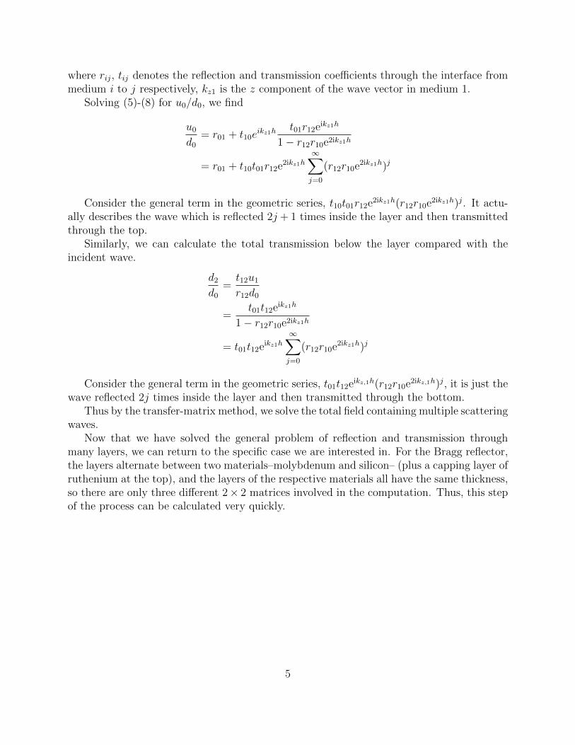
where rij, tij denotes the reflection and transmission coefficients through the interface frommedium i to j respectively, kz1 is the z component of the wave vector in medium 1.

Solving (5)-(8) for u0/d0, we find

u0

d0

= r01 + t10eikz1h

t01r12eikz1h

1− r12r10e2ikz1h

= r01 + t10t01r12e2ikz1h

∞∑j=0

(r12r10e2ikz1h)j

Consider the general term in the geometric series, t10t01r12e2ikz1h(r12r10e2ikz1h)j. It actu-ally describes the wave which is reflected 2j + 1 times inside the layer and then transmittedthrough the top.

Similarly, we can calculate the total transmission below the layer compared with theincident wave.

d2

d0

=t12u1

r12d0

=t01t12eikz1h

1− r12r10e2ikz1h

= t01t12eikz1h

∞∑j=0

(r12r10e2ikz1h)j

Consider the general term in the geometric series, t01t12eikz,1h(r12r10e2ikz,1h)j, it is just thewave reflected 2j times inside the layer and then transmitted through the bottom.

Thus by the transfer-matrix method, we solve the total field containing multiple scatteringwaves.

Now that we have solved the general problem of reflection and transmission throughmany layers, we can return to the specific case we are interested in. For the Bragg reflector,the layers alternate between two materials–molybdenum and silicon– (plus a capping layer ofruthenium at the top), and the layers of the respective materials all have the same thickness,so there are only three different 2× 2 matrices involved in the computation. Thus, this stepof the process can be calculated very quickly.

5

3 Transmission Matrix for the Absorber

In this section, we describe difraction of S-polarized plane waves by an absorbing body. Letus consider an absorber that stretches infinitely along the y-axis and has a rectangular cross-section in the xz-plane. Let us also assume that the incident plane wave hits the absorberat a small angle. The geometry for the S-polarized waves and an infinitely long absorber issimple; however, the ideas we describe here form a building block for simulating diffractionin more complicated settings.

Ein

Eout

θ

E(j)

E(j+1)

z

x

Figure 3: Sliced absorber with incident and transmitted waves (left). Incomming and out-going waves on (j + 1)st slice.

We use a perturbation approach to solving for the electromagnetic field known as theBorn approximation. Let us note, however, that we adapt the method for our needs. Tomake sure the Born approximation is accurate, we need to take care of two things. First,we assume that permittivity of the absorber is nearly the same as that of the vacuum. Thisallows us to use the solutions of Maxwell’s equations as a leading order contribution to thesolution. Next, to make sure the variation of the field is small in our solution scheme, wesuccessively find the solution on boundaries of thin rectangular slices of the absorber movingdown along the z-axis (see Figure 3).

3.1 Perturbation Approach

As an electromagnetic wave propagates along the absorber, it experiences only small variationin each of the slices shown on Figure 3. Using the perturbation techniques we derive a methodfor computing the field inside each slice given the field at its top surface.

Let us assume that the permittivity of the absorber, ε, is varying only in the x and zdirections. The electromagnetic field is governed by the time-harmonic Maxwell’s equations

6

∇×E = iωµ0H (9)

∇×H = −iωεE (10)

where permittivity is ε = ε0 + δε, and ε0 and µ0 are constant permittivity and permeabilityof vacuum. Assuming that |δε| ε0, let us look for E and H in a small neighborhood of theincident field E0, H0. Let us write the solution in the form E = E0 + δE, H = H0 + δH ,where E0, H0 are the electromagnetic waves in vacuum satisfying

∇×E0 = iωµ0H0 (11)

∇×H0 = −iωε0E0 (12)

Taking the curl of (12) we find that E0 is divergence-free. Now, using equations (9) and(10) for the free field, we rewrite (9) and (10) in the following form:

∇× δE = iωµ0δH (13)

∇× δH = −iω (ε0δE + E0δε+ δε · δE) (14)

For a thin slice, δE is small, so we can drop the second-order term δε · δE. By takingthe curl of (13), we eliminate the magnetic field and find the equation for the first ordercorrection to the E-field:

∇×∇× δE = ω2µ0ε0δE + ω2µ0E0δε (15)

Taking the divergence of (14) we find that

∇ · δE = − 1

ε0E0 · ∇δε

Since the incident field E0 is S-polarized and ∇δε lies in xz-plane, we have E0 · ∇δε = 0.Finally, using the identity ∇ × ∇ × δE = −∆δE + ∇(∇ · δE), we reduce equation (15) tothe Helmholtz equation (

∆ + k20

)δE = −k2

0

δε

ε0E0 (16)

where k0 = 2π/λ is the wave number of the incident wave. Clearly, this equation canbe solved using the Green’s function for the operator ∆ + k2

0, thus providing the solutionE = E0 + δE in the first slice.

It is important to point out that equation (16) can be used to solve for the field in a slabof absorber. Let zj denote the height of the jth slice top surface, with j increasing as wego down along z-axis. Let us also decompose the electromagnetic field and permittivity in

7

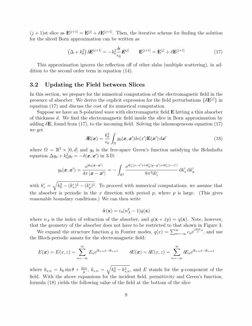
(j + 1)st slice as E[j+1] = E[j] + δE[j+1]. Then, the iterative scheme for finding the solutionfor the sliced Born approximation can be written as(

∆ + k20

)δE[j+1] = −k2

0

δε

ε0E[j] E[j+1] = E[j] + δE[j+1] (17)

This approximation ignores the reflection off of other slabs (multiple scattering), in ad-dition to the second order term in equation (14).

3.2 Updating the Field between Slices

In this section, we prepare for the numerical computation of the electromagnetic field in thepresence of absorber. We derive the explicit expression for the field perturbations δE[j] inequation (17) and discuss the cost of its numerical computation.

Suppose we have an S-polarized wave with electromagnetic field E hitting a thin absorberof thickness d. We find the electromagnetic field inside the slice in Born approximation byadding δE, found from (17), to the incoming field. Solving the inhomogeneous equation (17)we get

δE(x) =k2

0

ε0

∫Ω

g0(x,x′)δε(x′)E(x′) dx′ (18)

where Ω = R2 × [0, d] and g0 is the free-space Green’s function satisfying the Helmholtzequation ∆g0 + k2

0g0 = −δ(x,x′) in 3-D:

g0(x,x′) =eik0|x−x′ |

4π |x− x′|= −

∫R2

eik′x(x−x′)+ik′y(y−y′)+ik′z |z−z′ |

8π2ik′zdk′x dk′y

with k′z =√k2

0 − (k′x)2 − (k′y)

2. To proceed with numerical computations, we assume that

the absorber is periodic in the x direction with period p, where p is large. (This givesreasonable boundary conditions.) We can then write

δε(x) = ε0(n2A − 1)q(x)

where nA is the index of refraction of the absorber, and q(x + xp) = q(x). Note, however,that the geometry of the absorber does not have to be restricted to that shown in Figure 3.

We expand the structure function q in Fourier modes, q(x) =∑∞

n=−∞ cnei 2πnpx, and use

the Bloch-periodic ansatz for the electromagnetic field:

E(x) = E(x, z) =∞∑

n=−∞

Eneikx,nx−ikz,nz δE(x) = δE(x, z) =∞∑

n=−∞

δEneikx,nx−ikz,nz

where kx,n = k0 sin θ + 2πnp

, kz,n =√k2

0 − k2x,n, and E stands for the y-component of the

field. With the above expansions for the incident field, permittivity and Green’s function,formula (18) yields the following value of the field at the bottom of the slice

8

δE(x, z) = −k20(n2

A − 1)

∫Ω

∫R2

eik′x(x−x′)+ik′y(y−y′)+ik′z |z−z′ |

8π2ik′z

∞∑m,n=−∞

cmEneikx,n+mx′−ikz,nz′ dk′x dk′y dx′

= −k20(n2

A − 1)

8π2i

∞∑m,n=−∞

∫ d

0

∫R2

ei(k′xx+k′yy+k′z |z−z′ |−kz,nz′)cm−nEn(2π)2δ(kx,m − k′x)δ(−k′y)dk′x dk′yk′z

dz′

= −k20(n2

A − 1)

2i

∞∑m,n=−∞

cm−nEneikx,mx−ikz,mz

kz,m

∫ d

0

ei(kz,m−kz,n)z′ dz′ ( z′ > z )

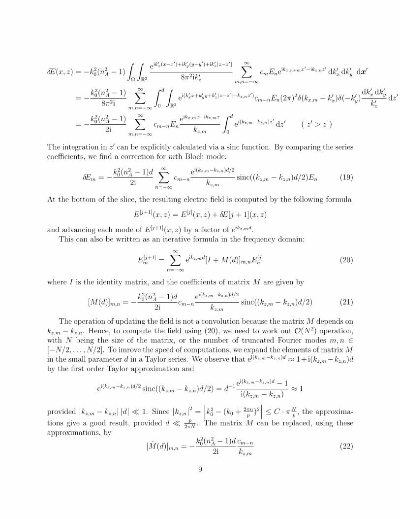
The integration in z′ can be explicitly calculated via a sinc function. By comparing the seriescoefficients, we find a correction for mth Bloch mode:

δEm = −k20(n2

A − 1)d

2i

∞∑n=−∞

cm−nei(kz,m−kz,n)d/2

kz,msinc((kz,m − kz,n)d/2)En (19)

At the bottom of the slice, the resulting electric field is computed by the following formula

E[j+1](x, z) = E[j](x, z) + δE[j + 1](x, z)

and advancing each mode of E[j+1](x, z) by a factor of eikz,md.This can also be written as an iterative formula in the frequency domain:

E[j+1]m =

∞∑n=−∞

eikz,md[I +M(d)]m,nE[j]n (20)

where I is the identity matrix, and the coefficients of matrix M are given by

[M(d)]m,n = −k20(n2

A − 1)d

2icm−n

ei(kz,m−kz,n)d/2

kz,msinc((kz,m − kz,n)d/2) (21)

The operation of updating the field is not a convolution because the matrix M depends onkz,m − kz,n. Hence, to compute the field using (20), we need to work out O(N2) operation,with N being the size of the matrix, or the number of truncated Fourier modes m,n ∈[−N/2, . . . , N/2]. To imrove the speed of computations, we expand the elements of matrix Min the small parameter d in a Taylor series. We observe that ei(kz,m−kz,n)d ≈ 1+i(kz,m−kz,n)dby the first order Taylor approximation and

ei(kz,m−kz,n)d/2 sinc((kz,m − kz,n)d/2) = d−1 ei(kz,m−kz,n)d − 1

i(kz,m − kz,n)≈ 1

provided |kz,m − kz,n | |d| 1. Since |kz,n |2 =∣∣∣k2

0 − (k0 + 2πnp

)2∣∣∣ ≤ C · πN

p, the approxima-

tions give a good result, provided d p2πN

. The matrix M can be replaced, using theseapproximations, by

[M(d)]m,n = −k20(n2

A − 1)d

2i

cm−nkz,m

(22)

9

The computation of the field with this matrix involves O(N log2N) operations.

Figure 4: The simulation of real parts of the total field obtained by sliced Born and FEMwith incident wavelength 13.5 nm only containing a single mode 0 in Fourier space. Thescatterer is a periodic array of 60 nm thick, 80 nm wide, infinitely long strips of TaBN(nA = 0.91654 + 0.04375i), with period 200 nm, the angle of incidence being 6 deg. NoBragg reflector is present.

Comparing the result of the sliced Born approximation with FEM, the profiles are quitesimilar; we show the error between them in figure 5. The first two figures are generatedby the Born approximation with the exact matrix (21). The solution of the sliced Bornapproximation converges as the number of slices is increased and the absolute error of thesetwo methods decreases. However, the error stagnates at 5% of the incident field amplitudewhen there are more than 50 slices. This illustrates that the sliced Born approximation givesus a convergent solution with some small error (< 10−1). Running time increases a littlebit, but not significantly, for more slices. The last two figures in figure 5 are generated bythe sliced Born approximation with the approximate matrix (22). Since we can write thisoperation as a convolution, the running time is decreased while the convergence rate anderror remain almost the same.

Figure 5: The comparison of the sliced Born and FEM simulations of transmitted fieldspassing through the absorber (with no Bragg reflector), and the convergent tests for thesliced Born with fixed number of Fourier modes. The sliced Born iteration is applied by thematrix (21) (left) and (22) (right).

10

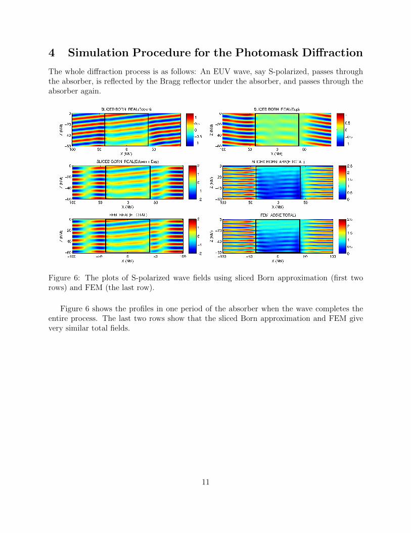
4 Simulation Procedure for the Photomask Diffraction

The whole diffraction process is as follows: An EUV wave, say S-polarized, passes throughthe absorber, is reflected by the Bragg reflector under the absorber, and passes through theabsorber again.

Figure 6: The plots of S-polarized wave fields using sliced Born approximation (first tworows) and FEM (the last row).

Figure 6 shows the profiles in one period of the absorber when the wave completes theentire process. The last two rows show that the sliced Born approximation and FEM givevery similar total fields.

11

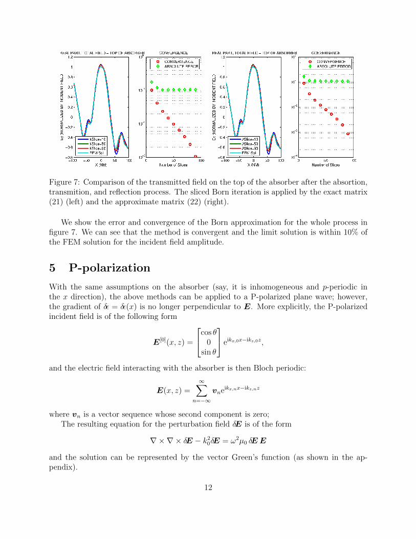
Figure 7: Comparison of the transmitted field on the top of the absorber after the absortion,transmition, and reflection process. The sliced Born iteration is applied by the exact matrix(21) (left) and the approximate matrix (22) (right).

We show the error and convergence of the Born approximation for the whole process infigure 7. We can see that the method is convergent and the limit solution is within 10% ofthe FEM solution for the incident field amplitude.

5 P-polarization

With the same assumptions on the absorber (say, it is inhomogeneous and p-periodic inthe x direction), the above methods can be applied to a P-polarized plane wave; however,the gradient of δε = δε(x) is no longer perpendicular to E. More explicitly, the P-polarizedincident field is of the following form

E[0](x, z) =

cos θ0

sin θ

eikx,0x−ikz,0z,

and the electric field interacting with the absorber is then Bloch periodic:

E(x, z) =∞∑

n=−∞

vneikx,nx−ikz,nz

where vn is a vector sequence whose second component is zero;The resulting equation for the perturbation field δE is of the form

∇×∇× δE − k20δE = ω2µ0 δEE

and the solution can be represented by the vector Green’s function (as shown in the ap-pendix).

12

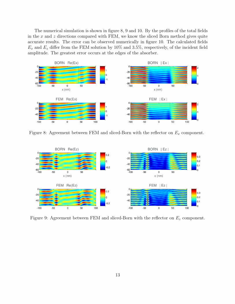
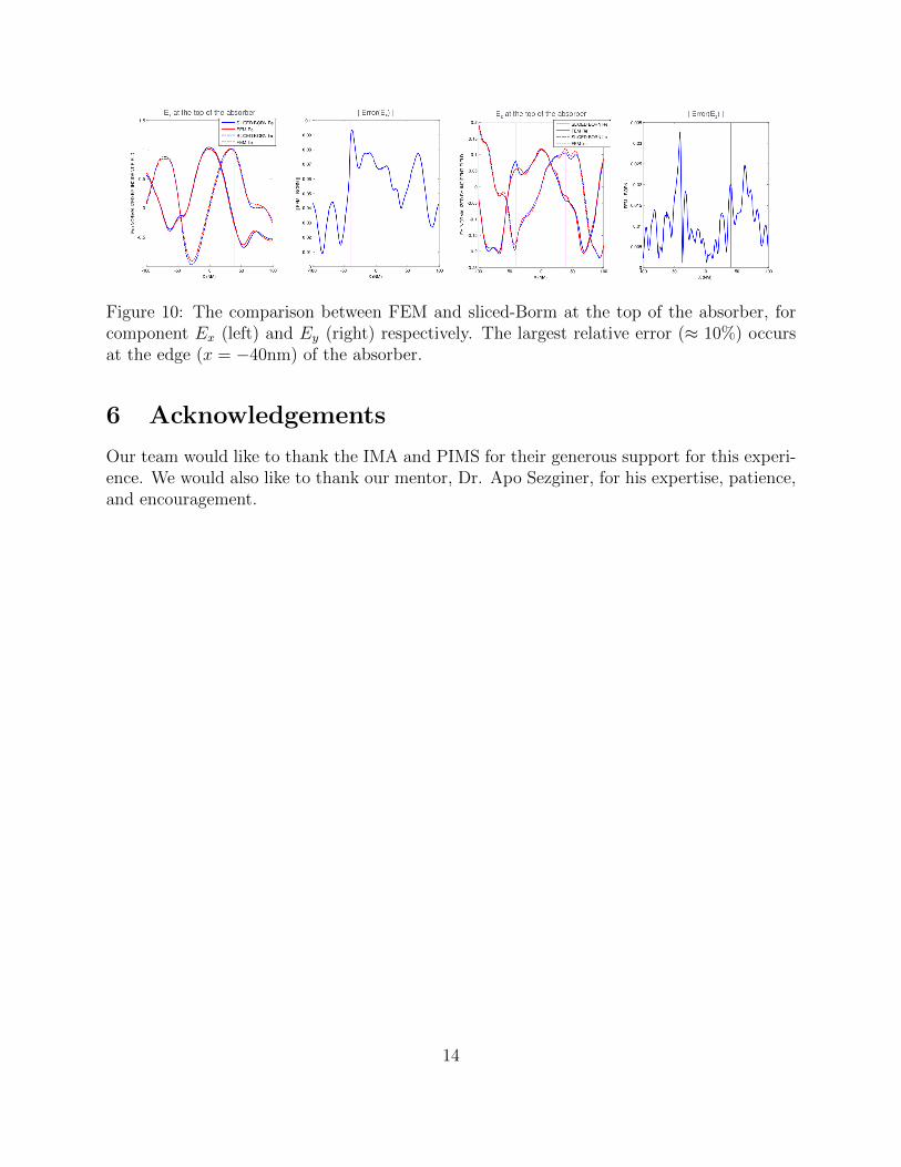
The numerical simulation is shown in figure 8, 9 and 10. By the profiles of the total fieldsin the x and z directions compared with FEM, we know the sliced Born method gives quiteaccurate results. The error can be observed numerically in figure 10. The calculated fieldsEx and Ez differ from the FEM solution by 10% and 3.5%, respectively, of the incident fieldamplitude. The greatest error occurs at the edges of the absorber.

Figure 8: Agreement between FEM and sliced-Born with the reflector on Ex component.

Figure 9: Agreement between FEM and sliced-Born with the reflector on Ez component.

13

Figure 10: The comparison between FEM and sliced-Borm at the top of the absorber, forcomponent Ex (left) and Ey (right) respectively. The largest relative error (≈ 10%) occursat the edge (x = −40nm) of the absorber.

6 Acknowledgements

Our team would like to thank the IMA and PIMS for their generous support for this experi-ence. We would also like to thank our mentor, Dr. Apo Sezginer, for his expertise, patience,and encouragement.

14

A Appendix

A.1 Helmholtz Equations for Time Harmonic Maxwell Equations

Let’s begin with the free space time-harmonic Maxwell equation with a current source J :

∇×E = iωµ0H (23)

∇×H = −iωε0E + J (24)

where ε0 = 8.85×10−3[F/nm] and µ0 are constant permittivity and permeability in vacuum.Taking divergence of (23) gives ∇ ·H = 0, and thus

H = ∇×A (25)

where A is a vector potential, and (23) yields ∇× (E − iωµ0A) = 0, or equivalently

E − iωµ0A = −∇φ (26)

for some scalar potential φ. Note that (A, φ) determines (E,H).Now take the curl of (24):

∇×H = ∇×∇×A = ∇(∇ ·A)−∆A

= −iωε0(iωµ0A−∇φ) + J .

By rearranging the terms and imposing the Gauge condition

∇ ·A− iωε0φ = 0 (27)

we have

(∆ + k20)A = −J (28)

By taking divergence on (26), we see that

∇ ·E − iωµ0∇ ·A = −∆φ

By (27) and taking ∇· on (24), it gives

(∆ + k20)φ = −∇ ·E = −∇ · J

iωε0(29)

Equations (28) and (29) are Helmholtz equations, whose solution can be represented bythe Green’s function

A(x) =

∫g(x,x′)J(x′) dx′

φ(x) =1

iωε0

∫g(x,x′)∇′ · J(x′) dx′

15

where g(x,x′) = g(x− x′) is the Green’s function for free space Helmholtz equation

(∆ + k20)g = −δ

Once A and φ are solved, E and H are solved by their definition (26), (25). Note that, bythe divergence theorem and the relation ∇′g(x,x′) = −∇g(x,x′), we have

∇∫g(x,x′)∇′ · J(x′) dx′ = −∇

∫(∇′g(x,x′)) · J(x′) dx′ = +∇

∫∇g(x,x′) · J(x) dx′

So we have

E(x) = iωµ0

∫ [(I +∇∇k2

0

)g(x,x′)

]J(x′) dx′ (30)

H(x) =

∫[∇g(x,x′)×]J(x′) dx′. (31)

A.2 Green’s Function for 1D Helmholtz Equation

The 1D Helmholtz Equation is indeed an ODE, and the Green’s function satisfies

d2

dz2g + k2g = −δ(z)

The solution g is

g(z) =eik|z |

−2ik

(One may check ddz|z | = sgn(z), d

dzsgn(z) = 2δ(z), and d

dzg = sgn(z)

−2eik|z |, d2

dz2g = −δ(z) +

ik−2

eik|z |.)

A.3 Green’s Function for 3D Helmholtz Equation

Now consider ∆g + k20g = −δ(x). To solve this, by taking Fourier transform w.r.t x and y

to the equation, it leads to

(∆ + k20)

∫∫eikxx+ikyyg(kx, ky, z) dkx dky = −δ(z)

∫∫eikxx+ikyy

4π2dkx dky

or equivalently∂2

∂z2g + k2

z g = −δ(z)

4π2k2z = k2

0 − k2x − k2

y

By Green’s function in 1D, we know g(kx, ky, z) = eikz |z |−2ikz

, and thus

g(x) =

∫∫eikxx+ikyy+ikz |z |

−8π2ikzdkx dky =

eik0‖x‖

4π ‖x‖kz =

√k2

0 − k2x − k2

y

‖x‖ =√x2 + y2 + z2

16

A.4 The Vector Green’s Function

The Green’s matrix G(x,x′) =[(I + ∇∇

k20

)g(x,x′)

]for (30) has the Fourier integral repre-

sentation

G(x,x′) = −∫∫

R2

ei(kx(x−x′)+ky(y−y′)+kz |z−z′ |)

8π2ikzdkx dky

where kz =√k2

0 − k2x − k2

y and

K =

1− k2

x

k20

−kxkyk20

−kxkzk20

sgn(z − z′)

−kxkyk2

0

1− k2yk20

−kykzk20

sgn(z − z′)

−kxkzk2

0

sgn(z − z′) −kykzk20

sgn(z − z′) 1− k2zk20

+ 2ikzk2δ(z − z′)

References

[1] F. Natterer, “An error bound for the Born approximation.” Inverse Problems 20 (2004),447-452.

[2] N. P. K. Cotter, T. W. Preist, and J. R. Sambles, “Scattering-matrix approach tomultilayer diffraction.” J. Opt. Soc. Am. A 12 (2004), 1097-1103.

17