DIFFUSION DRIVEN INSTABILITY IN AN …jas/paperpdfs/debbie1.pdf · Diffusion driven instability in...

Bulletin of Mathematical Biology Vol. 55. No. 2, pp. Printed in Great Britain.

365-384,1993. 0092-8240/93S6.00 + 0.00

Society for Pergamon Press Ltd

Mathematical Biology

DIFFUSION DRIVEN INSTABILITY IN AN INHOMOGENEOUS DOMAIN

n DEBBIE L. BENSON, JONATHAN A. SHERRATT and.PHILIP K. MAINI Centre for Mathematical Biology, Mathematical Institute, 24-29 St Giles’, Oxford OX1 3LB, U.K. (Email: [email protected])

Diffusion driven instability in reaction-diffusion systems has been proposed as a mechanism for pattern formation in numerous embryological and ecological contexts. However, the possible effects of environmental inhomogeneities has received relatively little attention. We consider a general two species reactiondiffusion model in one space dimension, with one diffusion coefficient a step function of the spatial coordinate. We derive the dispersion relation and the solution of the linearized system. We apply our results to Turing-type models for both embryogenesis and predator-prey interactions. In the former case we derive conditions for pattern to be isolated in one part of the domain, and in the latter we introduce the concept of “environmental instability”. Our results suggest that environmental inhomogeneity could be an important regulator of biological pattern formation.

1. Introduction. Reaction-diffusion mechanisms form perhaps the most widely studied class of models for biological pattern formation, and have been successfully applied to a wide range of developmental and ecological systems. All such models are ultimately based on Turing’s (1952) seminal work on “the chemical basis of morphogenesis”, and more recent applications to embryogenesis utilize Wolpert’s (1969, 198 1) concept of positional information. Wolpert suggested that cells are pre-programmed to differentiate according to local concentrations of chemical morphogens, thereby translating a con- tinuous chemical pre-pattern into a discrete pattern of different cell types. There is now considerable literature on applications of this idea to a wide range of developmental problems (see the references in the books by Meinhardt, 1982; Murray, 1989). Segel and Jackson (1972) first proposed diffusion driven instability as an explanation for the spatial heterogeneity that is sometimes observed in predator-prey interactions. Again, the idea that dispersal could give rise to instabilities and thence to spatial pattern was built on by a number of authors (see Okubo, 1980, for review).

One feature common to the vast majority of these applications of diffusion driven instability is that they are considered in the context of a homogeneous environment, so that the model parameter values are constant across the

365

366 D. L. BENSON et al.

domain. However, environmental variation may be an important regulator in some biological systems. The influence of the local topography on population dispersal has long been recognized, and a number of authors have studied this using spatially discrete models (see, for example, Levin 1976, 1986). In developmental biology, considerations of scale invariance have led to the suggestion that morphogen diffusivity might be controlled by the concentration of a non-reacting regulatory chemical, which could result in a spatial variation (Othmer and Pate, 1980; Pate and Othmer, 1984; Hunding and Sorenson, 1988).

In this paper we present a mathematical analysis of the spatial patterns implied by reactiondiffusion mechanisms in which the dispersal rate of one species varies in a simple stepwise manner across the domain. We consider applications of our results in both embryology and ecology. Despite the extensive mathematical literature on reaction-diffusion equations (for review, see the books by Britton, 1986; Murray, 1989), we are not aware of previous attempts to analyse patterns in this case. Auchmuty and Nicolis (1975) analyse a system in which the reaction terms depend explicitly on space, and investigations of the effects of spatial varying parameters in ecological reaction-diffusion models have focused on carrying capacities and other parameters in the reaction terms (Pacala and Roughgarden, 1982; Shigesada, 1984; Cantrell and Cosner, 1991).

2. Conditions for Diffusion Driven Instability. Homogeneous environment. We begin by summarizing the conditions for

diffusion driven instability in a homogeneous environment; a detailed derivation of the results can be found, for example, in the book by Murray (1989). We consider a two species reaction diffusion system in one space dimension, with the form:

dU -= at

D a% up+fh u)

av at

(1 1 a

(Ib)

where D, and D, are positive constants, and where the reaction termsfand g are such that a non-zero homogeneous steady state (u,, vO) exists. For simplicity, we consider these equations on a finite domain, [0, l] say, with zero flux boundary conditions. This system exhibits diflusion driven instabibty if the homogeneous steady state (uO, vJ is stable to spatially homogeneous perturbations, but unstable to some inhomogeneous perturbations. The

DIFFUSION DRIVEN INSTABILITY 367

conditions for this phenomenon, and thus for the generation of spatial pattern, are:

a+d<O

ad>bc

D,a+D,d>O

(D,a + D,d)2 >4D,,D,(ad - bc),

where

af b af dg a = Ji (uo uo)

=- 7

al (uo uo) c = z-4 (uo 00)

d a’ =-

al l , , (UOJJO)

(2 ) a

VW (2 1 C

(2d)

The set of parameter values satisfying these conditions is known as the TUring space. One important implication of (2a, b, c) is that:

ad<0 and bc<O, (4)

so that within an arbitrary relabelling of species, the kinetic matrix has one of two forms:

+ - ( > + - + + ( > - - pure activator-inhibitor model cross activator-inhibitor model.

In the former case, solutions for the two species will be in phase, while in the latter case they will be out of phase, at least in the vicinity of a primary bifurcation point (Dillon et al., 1992).

Inhomogeneous environment. We now amend the standard system (1) by replacing the dispersal term in (lb) by (a/ax) [D(x)&@x], where:

and &z(O, 1); we assume that D-<D+. Thus the domain is composed of two parts, with the diffusion coefficient of u the same, but that of v different, on the two parts. This represents the simplest possible case of environmental variation in diffusivity, and our analysis in this simple case provides an understanding of the way in which environmental inhomogeneities can modulate the ?aattern- forming capabilities of reaction-diffusion systems. Moreover, as dissussed


below, numerical solutions of models with more realistic forms for D(x) reveal qualitatively similar patterns to those predicted when D(x) is a step function.

For this inhomogeneous model, we ask: what are the amended conditions for diffusion driven instability, and what is the form of the patterns generated when these conditions are satisfied? The requirements for (uO, v,) to be stable to spatially homogeneous perturbations remain (2a) and (2b). .To derive the analogues of (2~) and (2d), we linearize the model about the steady state ( z+,, z+,), and look for separable solutions of this linearized system, in the form u -u. = e”‘X,(x), v - v. = eA’XV(x). Substituting these into the linearized model gives coupled ordinary differential equations for X, and Xv:

Xz+(a-3L)XU+bX,=0

[D(x)xJ + cxu + (d - 1)X” = 0;

here prime denotes d/dx. We consider these equations separately on [0, <) and (r, 11. In the former case, adding (6a) to s -/D - times (6b) gives:

We choose s- such that:

b+(d-;l)s-/D- _ a-?+cs-/D- =’ ’

which is a quadratic equation for s -, with roots SF and ST, say. Equation (7) then becomes a single equation in X, + Sj- X”, for j = 1,2, with general solution Cj COS(~~~X) + Dj sin&:x). Here Cj and Dj are constants of integration, and ai =[a-II+csJD-]‘/2, j= 1,2. We therefore have two simultaneous equations for X,(x) and X,(x) in [0, 0. Solving these and applying zero flux boundary conditions at x = 0 gives:

x,(x) = 1 - (

- a s2 -0 i

K+G-T,)si- cos(a,x) K+s;T,)s, cos(a,x) Wror,) wrcc, 1 1 (9 1

, x,(x) = 1 -

( -

s2 [ (ru+si-rv) cos(a,x)

-s1-) cos(&-) (ru+sx) cos(a,x) cos(ra,) 1 cw

on [0, t), where IU= X,(r), IV= X,(& In (9a,b), we are assuming that S; #s;


solutions for u and u cannot in general satisfy continuity of flux at x = 5. One notable exception to this, however, is the homogeneous case D - = D +. The solutions of the dispersion relation given by the standard analysis (see above and Murray, 1989) satisfy ~j’ = ~171: for some no [l, 2, 3, . . .} and eitherj= 1 or j= 2. Thus with < = l/2, half of the eigenvalues 1 are not roots of (1 l), since cos(n42) = 0 when y1 is even. These roots can be retrieved, however, either by investigating the above special cases, or by taking more general values of l: the value of t is irrelevant when D - = D + .

In general the roots of the dispersion relation (11) are complex. However, when the diffusion coefficients are spatially homogeneous, all solutions of the dispersion relation with non-zero imaginary parts have negative real parts. Moreover, our numerical solutions of the partial differential equation system in the case of a step function diffusivity have never revealed time periodic instabilities, which would be implied by Im(3,) #O. Therefore we assume that the solutions of (11) which have positive real part are real and we restrict attention to real values of A. Although (11) cannot be solved analytically, it is amenable to simple numerical solution in this case, since when ALE IR, straightforward algebra shows that F(A) is also real valued. A typical functional form of F(A) is illustrated in Fig. 1. Fhas infinities at values of 3L for which one of cos(~cQ, cos(&x,), cos((l- t)cr,+), cos((1 -C;Y)ciz) or (si -s,‘) is zero; as explained above, our linear solutions are not valid for these values of A. It is not immediately clear from (11) that conditions (4) must hold for diffusion driven instability to be possible in the amended system. However, numerical solutions of (11) suggest that, as expected intuitively, these conditions are still necessary for diffusion driven instability. Thus the classification of models exhibiting diffusion driven instability into pure and cross activator-inhibitor models remains valid.

3. Applications. The Schnackenberg model for morphogenesis. One of the most widely

studied reaction diffusion models for Turing-type pattern formation in embryogenesis is that proposed by Schnackenberg (1979), which is based-on a hypothetical mechanism consisting of a series of trimolecular autocatalytic reactions involving two chemicals. When appropriately nondimensionalized in one space dimension with a step function diffusion coefficient for the inhibitor chemical, the model equations are:

au a221 dt=axz+ y(A-u+u”v)

au d at=ax D(x); + y(B-u2v) [ 1

(124


x Figure 1. A typical functional form of the dispersion relation F(L), defined in (1 l), for the Schnackenberg system (12), with parameter values in the Turing space. For clarity, we plot sign (F) - log(1 + IFI) on the vertical axis, to better illustrate the infinities of F(li). The parameter values are y = 1040, A = 0.1, B= 0.9, D - = 7, D+ = 12, 5 =OS. In this particular case there are two unstable modes, with approximate linear growth rates R = 34.9 and ;1= 104.4. For all parameter values, a

straightforward calculation shows that F(A) = O(A) as R+ co.

on <X < 1. Here A and B are positive constants and y is a scale parameter proportional to the dimensional length of the domain; the step function D(x) is defined in (5). This is a cross activator-inhibitor model. Again, for simplicity we consider only zero flux boundary conditions. This system has a single homogeneous steady state, at U- A + B, v= B/(A + B)2, which is stable to homogeneous perturbations provided (A + B) 3 > B - A; all the numerical results we will show use parameter values satisfying this condition.

The dispersion relation (11) enables us to determine numerically the Turing space for (12). As expected intuitively, whenever D + > D - > Dcrit 3 the model exhibits diffusion driven instability; here Dcrit is the value that a spatially homogeneous diffusion coefficient must exceed for diffusion driven instability. When D - < Dcrit, however, diffusion driven instability requires D+ to be greater than a critical value, O,~i, say, which depends on A, B, y and D -. The variation Of D,‘,i, with D - is illustrated in Fig. 2 for typical values of A, B and y: as expected, Digit approaches Dcrit from above as D- approaches Dcrit from below. These calculated values compare very well with results from numerical simulations using the full partial differential equation model. The form of these conditions depends crucially on a being positive, so that d is negative. If these signs are reversed, all the inequalities are reversed, and this corresponds to denoting the activator and inhibitor chemicals, respectively, by v and u rather than u and v.


D - . crit

D-

Figure 2. The parameter space for the reaction diffusion system (12). The diffusion coefficient of the species u is constant throughout the domain, while that of u has the constant value D - on [0, r) and D + on (5, 1 J. For parameters in region I, diffusion driven instability gives rise to type A isolated patterns (see text for details). In region II patterns are either type B isolated patterns or (for larger values of D * ) non-isolated patterns; the division between these types is arbitrary. In region III, D+ < Deli, and thus the system does not exhibit diffusion driven instability. In the shaded region, D - > D + ; this is therefore not a valid region of parameter space. In both of the regions I and II, the solution is in category (bi) on (r, 1 J, while on [0, 0 the solution is in category (bii) in region I and in category (a) or (bi) in region II. The other parameter values used in the figure are y = 1040, r =OS, A = 0.1, 8=0.9. These are the same parameters as those used in Fig. 3, and we indicate the position in this parameter domain of the solutions shown in the three parts of Fig. 3. For clarity, we show only the portion 7 \< D + < 10.5 of the D +-axis, but our conclusions are valid for a wide range of values of D +. To better illustrate the interesting behaviour when D- is small, we use a magnified linear horizontal scale on

OdD- ~0.5.

In the vicinity of a primary bifurcation point with a simple spatial eigenvalue, the key qualitative features of the patterns given by the full non-linear system are generally captured by the separable solution of the model when linearized about the homogeneous steady state, with the eigenvalue 1 taken as the largest real solution of the dispersion relation. Now in the course of deriving the dispersion relation (1 l), we have obtained the separable solutions of the linearized system corresponding to (12), and the spatial part of these solutions is given in (9). As in the homogeneous case, with il as the largest real solution of the dispersion relation (1 l), the linear solution captures the key qualitative features of the non-linear patterns predicted by our model (12), for a wide range of parameter values (Fig. 3).

A major difference between the patterns illustrated in Fig. 3 and those familiar from spatially homogeneous reaction diffusion equations, is that for some parameter values, the pattern is isolated in one part of the domain. Now for given values of all the parameters, the concept of “isolated pattern” is not really meaningful, since by appropriately subdividing the domain, any pattern can be said to be restricted to particular subdomains. However, the key aspect of our model is that pattern remains isolated in a specific subdomain as the

r 1 Linear Solution 1

1.6

1.2 2 5

0.8

1.6

1.2 52 5

0.8

0.2 0.4 0.6 0.8 1

1 Linear Solution I

1 Linear Solution 1

1.6

1.2 2 5

0.8

0.2 0.k ok 0:s 1 X

> 0.8

0.6 )

fb)

1.0 ‘;; ‘5’

0.8

0.6 1

(4

6.8

-0.6

0

G y 1.0

0.8

1.1

G y 1.0

0.9

PDE solution

.so z

0.2 0.-4 0.6 O.-S 1.-O X

PDE solution

PDE solution I

0.2 0.4 0.6 0.8 1.0 X

Figure 3. Comparison of the linear solution (9) with the full solution of the Schnackenberg system (12) in different regions of the parameter space. (a) A type A isolated pattern, with D - = 0.1 and D + =9.2. (b) A type B isolated pattern, with D-=7andD+ = 10. (c) A non-isolated pattern, with D - = 8.4 and D + = 8.9. The other parameter values are A =O.l, B=0.9, y= 1040, c=O.5. The location of these solutions in the D- -D + parameter space is illustrated in Fig. 2. In each case the linear solution captures the qualitative behaviour of the full non-linear pattern. Note that the patterns for u and v are out of phase, since the Schnackenberg system is a cross activator-inhibitor model. The full non-linear model was solved numerically using the method of lines and Gear’s method (Gear, 1971) from initial conditions of small random perturbations about the homogeneous steady state, until a new inhomogeneous steady state was reached. The non-linear pattern thus obtained is independent of the initial perturbations (within a change in sign of both u -uO and v- vO) for all values of D ’ used in the figure. However for sufficiently large D+, there are several unstable modes with similar growth rates, and different

initial conditions result in qualitatively different patterns. (---------u; -v).

85


value of the scale parameter is varied, and in this sense the possible isolation of pattern is independent of the scale parameter y. This is in marked contrast to the homogeneous case, in which the number and position of concentration peaks varies with y for given values of the other parameters, so that pattern occurs in any subdomain for an appropriate value of y (see Murray, 1989 for .

’ Mathematically, we can divide isolated patterns into two types: . review).

Type A, As the scale parameter y varies (but is large enough that diffusion driven instability occurs), the model solution is always monotonic in one part of the domain, but is in general oscillatory in space elsewhere.

Type B. As y varies such that diffusion driven instability occurs, the model solution is in general oscillatory in space throughout the domain, but with much greater amplitude in one part of the domain than elsewhere.

We now use the linear solution (9) to drive necessary and sufficient conditions for the existence of type A isolated patterns. We begin by investigating the forms of these solutions: without loss of generality we consider only the region [0, <). There are then two cases to consider.

0 - a S, , S, complex conjugates. In this case, a, and U, are complex

conjugates, say ai + iq- . Note that the assumption s, #SF implies that or- ~0. Moreover, straightforward algebra shows that s;(r,+q-r,)/ C( sy -sJcos(5ay)] and sJI’~+s,T,)/[(s[ -s;)cos(&)], and also (IU+ %?-iJl(s, -s;)cos(~or~)] and (IU+s;I’J/[(s; -s;)cos(&~;)] are both complex conjugate pairs, say vu + iv,, and ylV Ifr iv,, respectively. In this notation, (9 ) a is:

Xu = (q, + iv,)cos[(a, + ia&] + (vu - iv,)cos[(a, - ic$-)x]

= 2q, cos(cr, x)cosh(a[ x) + 2v, sin& x)sinh(or,x)

= ~u(x)cos(cc,x + J!,(x)).

Similarly .

Here

xv = 9$(x)cos(tx,x + S”(X)).

t9 t(,v = k 2[qz,, cosh2(ai-x) + v:,~ sinh2(a,x)] ‘j2

.A? L(,t, = tan - 1 [ - tanh(or, x) * v,,,lq,,,] .

Thus YU &x) are the amplitude modulating functions, or envelopes, while s,,,(x) affects the wavelengths of oscillations.

Differentiating (13) with respect to x shows that ISI is monotonically


value of the scale parameter is varied, and in this sense the possible isolation of pattern is independent of the scale parameter y. This is in marked contrast to the homogeneous case, in which the number and position of concentration peaks varies with y for given values of the other parameters, so that pattern occurs in any subdomain for an appropriate value of y (see Murray, 1989 for review). Mathematically, we can divide isolated patterns into two types:

Type A. As the scale parameter y varies (but is large enough that diffusion driven instability occurs), the model solution is always monotonic in one part of the domain, but is in general oscillatory in space elsewhere.

Type B. As y varies such that diffusion driven instability occurs, the model solution is in general oscillatory in space throughout the domain, but with much greater amplitude in one part of the domain than elsewhere.

We now use the linear solution (9) to drive necessary and sufficient conditions for the existence of type A isolated patterns. We begin by investigating the forms of these solutions: without loss of generality we consider only the region CO,<). There are then two cases to consider.

( ) - a S, , S, complex conjugates. In this case, or, and a, are complex

conjugates, say ai + iccIV. Note that the assumption s, #sz implies that ccl ~0. Moreover, straightforward algebra shows that si- (r, + q- Tu)/ CC SF -s,)cos(&x,)] and sJI’~+s,T,)/[(s, -s;)cos(&)], and also (IU+ s1- Lm- -s;)cos(&;)] and (IU+s;T,)/[(s; -sJcos((a;)] are both complex conjugate pairs, say qU + iv, and ylo + iv,, respectively. In this notation, (9 ) a is:

Xu = (q, + iv,)cos[(a, + iaJx] + (q, - iv,)cos[(a, - iOr,)x]

= 217, cos(a&)cosh(alDx) + 2v, sin(a&)sinh(aix)

= Pu(x)cos(a~x + A!,(x)).

Similarly . X, = P&x)cos(agx + S,(x)).

Here 9 l(,o = f 2[qz,, cosh2(aIDx) + v& sinh2(arBx)] ‘I2

9 l(,o = tan- ’ [ - tanh(a,x) l v,,,IqJ.

(13)

Thus PU “(x) are the amplitude modulating functions, or envelopes, while 5!,,,(x) ahects the wavelengths of oscillations.

Differentiating (13) with respect to x shows that 191 is monotonically


increasing on [O, <), and thus in this case XU and XV are oscillatory functions with monotonically growing amplitude of oscillation.

(b) s[, s, real. There are three subcases to consider.

0 i 6-l , 012 real. Here we write: .

ov = C(L +4- r,)/cos(5q ) + (r, + s; rvycOs(ta; )]/~2(~; - s; )I

6, = CCL + sl- r,)/ws~; ) - (r, + s; rv)/cOs(~a; )]/~2(~; - s; )I.

With this notation, we can rewrite (9) in the form:

xu =~u(x)cos[~(a, + a,)x +9,(x)] xv = 9v(x)cos[+(a, + q-)x + S”(X)]

9 %V = *2{&fv cos2[+(ct; -a;)~] +a;l”v sin”[$(or, --a&]} U2 (14) 9 u,v= tan- ‘[tan[& -Qx] l 6,,,/6,,,].

Therefore, the solutions again have the form of oscillating functions with envelopes Pu,, and wavelength variations controlled by Su v. In this case, , however:

($) 8% v(x) u,v a;c = 2(cc, -a;)(--d,‘,)sin[(a+x;)x], ,

which is not necessarily of constant sign, so that the amplitude of successive concentration peaks may increase or decrease, depending on parameter values and position in the domain. The envelopes defined in (13) and (14) provide a simple representation of the way in which oscillating patterns vary in amplitude across the domain, as illustrated in Fig. 4.

. . ( 1 n cc,, cc; purely imaginary. Writing ai = i4i forj= 1,2, we have in this

case:

xu= _ 1 - G-w-i+s,T,)

cash 4,x cash q&-x

S2 -S1 [ cash c&-[ --~;(r~+~;r,)

cash &r 1 Wa) xv =

1 - -

S2 -%

. 1 Wb)


0.6

-0.4

-0.6

0.2 0.2

.

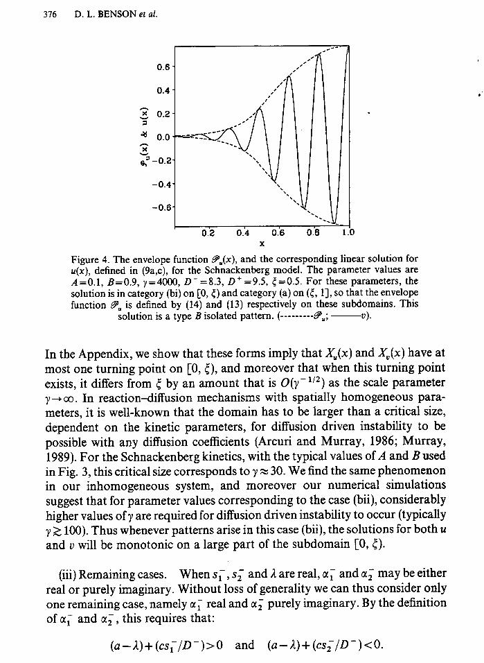
Figure 4. The envelope function g&c), and the corresponding linear solution for u(x), defined in (9a,c), for the Schnackenberg model. The parameter values are A=O.l, B=0.9, y=4000, D-=8.3, D+ = 9.5, 5 =OS. For these parameters, the solution is in category (bi) on [0, c) and category (a) on (c, 11, so that the envelope function PU is defined by (14) and (13) respectively on these subdomains. This

solution is a type B isolated pattern. (---------9,; ---?I).

In the Appendix, we show that these forms imply that X&) and XV(x) have at most one turning point on [0, [), and moreover that when this turning point exists, it differs from { by an amount that is O(y-‘12) as the scale parameter y- 00. In reaction-diffusion mechanisms with spatially .homogeneous parameters, it is well-known that the domain has to be larger than a critical size, dependent on the kinetic parameters, for diffusion driven instability to be possible with any diffusion coefficients (Arcuri and Murray, 1986; Murray, 1989). For the Schnackenberg kinetics, with the typical values of A and B used in Fig. 3, this critical size corresponds to y z 30. We find the same phenomenon in our inhomogeneous system, and moreover our numerical simulations suggest that for parameter values corresponding to the case (bii), considerably higher values of y are required for diffusion driven instability to occur (typically y 2 100). Thus whenever patterns arise in this case (bii), the solutions for both u and v will be monotonic on a large part of the subdomain [0, 5).

(iii) Remaining cases. When SF, ST and ;1 are real, a, and ai may be either real or purely imaginary. Without loss of generality we can thus consider only one remaining case, namely or, real and cc, purely imaginary. By the definition of CY[ and o(;, this requires that:

(a-A)+(csJD-)>O and (a-R)+(csJD-)<O.


Multiplying these inequalities and using the expressions for the sum and product of the roots of (8) gives:

R2-(a+d)l+(ad-bc)<O.

Conditions (2a) and (2b) imply that this inequality can never be satisfied when IL ~0. Thus in this case the system cannot exhibit diffusion driven instability.

This classification of patterns in the two subdomains [0, 5) and (5, I] into the three categories (a), (bi) and (bii) depends on whether $ and c$ are real or complex for j= 1,2. This is independent of the scale parameter y near the bifurcation point (see below). This remains true in numerical simulations for a wider range of parameter values. For type A isolated patterns, we therefore require that the linear solutions (9) be in category (bii) on [0, 5) and in category (a) or (bi) on (c, 11. F or t ype B isolated patterns we require the solutions to be of category (a) or (bi) on both parts of the domain. The distinction between type B isolated patterns and non-isolated patterns is arbitrary.

We will show below that whenever the system exhibits diffusion driven instability, the solution on (<, 1] is in category (bi). It is therefore necessary and sufficient for type A isolated patterns that SF, s, E R and a,, a, &DB. We investigate these conditions further by considering the case of marginal stability, that is a=0 and D + = O=~it. Then SF and SF are the roots of:

CS-2 +(D-a-d)s--D-b=0

and c$- = [a + csJD -1 ‘12, j = 1,2. We therefore require:

c (d-aD-)+{(D-a-d)2+4D-bc}1/2 O>a+D-.

2c .

(16)

(17)

Simplifying (17) gives:

which is satisfied if and only if both:

and

O>aD-+d (18)

O<(D-a+d)2-(D-a-d)2-4D-bc=4D-(ad-bc). (19)

Condition (2b) ensures that (19) is always satisfied. The inequality (16) is satisfied if and only if D - < 6 1 or D - > 6,, where 6, and 6, are the roots of a2S2+2(2bc-ad)S+d2- -0. The conditions (2a,b) and (4) imply that these roots are real, distinct and positive, say 6, > 6, ~0, and moreover that - d/aE (6,) 6,). Therefore (16) and (18) together give a single necessary and


sufficient condition for pattern to be isolated at marginal stability, which when a > 0, as in the Schnackenberg model, is:

0-d 1 =f [(ad-2bc)-2{bc(bc-ad)}1’2].

Numerical simulations for the Schnackenberg model continue to predict isolated patterns for D - < 6, when D + > Dc:i,. For D - slightly larger than 6,) the patterns at marginal stability are type B isolated patterns.

Straightforward manipulation of the inequalities (2a-d), which determine the critical spatially homogeneous diffusion coefficient Dcrit, shows that in fact D crit = 6,. At marginal stability, D + = D~it > Dcrit, SO that sc, SC E R and the solution is in category (bi) on (5, 11. Numerical simulations again suggest that this result remains valid when D + > Digit . Similarly, the solution is in category (bi) on [O, c) at marginal stability provided D- > Dcrit. The biological implications of this analysis will be discussed in Section 4.

Our analysis is based on a stepwise diffusion for a particular morphogen. This may be set up by a smooth gradient in a control chemical which affects morphogen diffusivity in a threshold manner. The phenomenon of isolated pattern does not depend critically on the step function nature of diffusion: numerical solutions indicate that a smoothly varying diffusion coefficient produces similar results (see Fig. 5).

0.8

I

- (b)

r 0.2 0.4 0.6 0.8 1.0

X X

Figure 5. The solution of the Schnackenberg system (12) for continuously varying D(x), the diffusion coefficient of the inhibitor chemical. (a) The form of D(x), which we take as D(x) = D, cosh(Ox), with D, and 6 chosen so that D(0) = 2 and D( 1 )= 14. (b) The corresponding steady state solution of (12). The system is solved numerically as in Fig. 3. The pattern is remarkably similar to those given when D(x)

is a step function (--------4; -II).


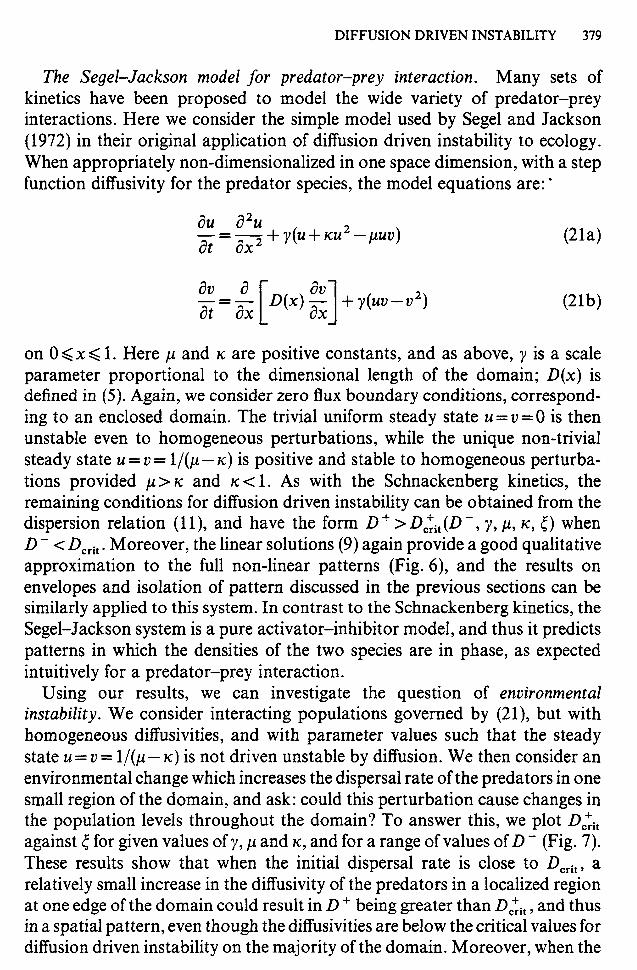
The Segel-Jackson model for predator-prey interaction. Many sets of kinetics have been proposed to model the wide variety of predator-prey interactions. Here we consider the simple model used by Segel and Jackson (1972) in their original application of diffusion driven instability to ecology. When appropriately non-dimensionalized in one space dimension, with a step function diffusivity for the predator species, the model equations are: l

du a2u -= -+ y(u+lcu2-puv) at ax2

dv a z=z D(x); + y(uv-v2) [ 1 cw

Plb)

on 0 \<x < 1. Here p and IC are positive constants, and as above, y is a scale parameter proportional to the dimensional length of the domain; D(x) is defined in (5). Again, we consider zero flux boundary conditions, corresponding to an enclosed domain. The trivial uniform steady state u = v=O is then unstable even to homogeneous perturbations, while the unique non-trivial steady state u = v = l/(p- K) is positive and stable to homogeneous perturbations provided p> K and IC < 1. As with the Schnackenberg kinetics, the remaining conditions for diffusion driven instability can be obtained from the dispersion relation (1 l), and have the form D + > D&(D -, y, p, K, <) when D - < Dcrit. Moreover, the linear solutions (9) again provide a good qualitative approximation to the full non-linear patterns (Fig. 6), and the results on envelopes and isolation of pattern discussed in the previous sections can be similarly applied to this system. In contrast to the Schnackenberg kinetics, the Segel-Jackson system is a pure activator-inhibitor model, and thus it predicts patterns in which the densities of the two species are in phase, as expected intuitively for a predator-prey interaction.

Using our results, we can investigate the question of environmental instability. We consider interacting populations governed by (21), but with homogeneous diffusivities, and with parameter values such that the steady state u = v = l/(p - K) is not driven unstable by diffusion. We then consider an environmental change which increases the dispersal rate of the predators in one small region of the domain, and ask: could this perturbation cause changes in the population levels throughout the domain? To answer this, we plot Dali, against c for given values of y, p and K, and for a range of values of D - (Fig. 7). These results show that when the initial dispersal rate is close to Dcrit, a relatively small increase in the diffusivity of the predators in a localized region at one edge of the domain could result in D + being greater than D,‘,i, , and thus in a spatial pattern, even though the diffusivities are below the critical values for diffusion driven instability on the majority of the domain. Moreover, when the


I Linear Solution I 1 PDE Solution 1

0.2 0.4 0.6 0.8 1

4.2 4.5 -

3.8

1 X

I I 0.2 0.4 0.6 0.8 1.0

X

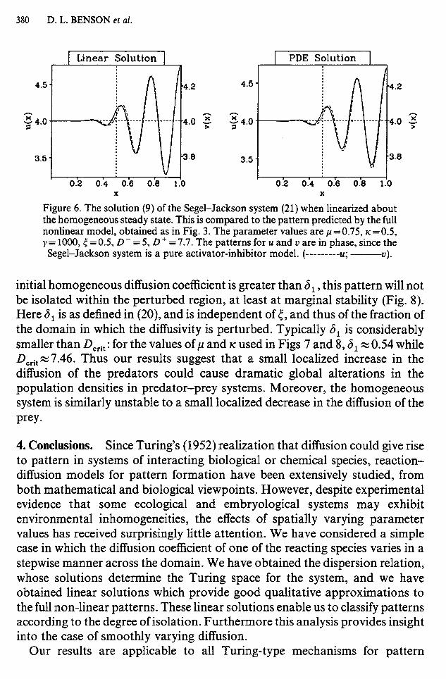
Figure 6. The solution (9) of the Segel-Jackson system (21) when linearized about the homogeneous steady state. This is compared to the pattern predicted by the full nonlinear model, obtained as in Fig. 3. The parameter values are p =0.75, K =OS, y=1000,~=0.5,D-=5,D+ = 7.7. The patterns for u and u are in phase, since the Segel-Jackson system is a pure activator-inhibitor model. (---------U; -------?I).

initial homogeneous diffusion coefficient is greater than 6,, this pattern will not be isolated within the perturbed region, at least at marginal stability (Fig. 8). Here 6, is as defined in (20), and is independent of 5, and thus of the fraction of the domain in which the diffusivity is perturbed. Typically 6, is considerably smaller than Dcrit : for the values of ,u and K used in Figs 7 and 8,6, ~0.54 while D 0,X7.46. Thus our results suggest that a small localized increase in the diffusion of the predators could cause dramatic global alterations in the population densities in predator-prey systems. Moreover, the homogeneous system is similarly unstable to a small localized decrease in the diffusion of the Prey l

4. Conclusions. Since Turing’s (1952) realization that diffusion could give rise to pattern in systems of interacting biological or chemical species, reaction- diffusion models for pattern formation have been extensively studied, from both mathematical and biological viewpoints. However, despite experimental evidence that some ecological and embryological systems may exhibit environmental inhomogeneities, the effects of spatially varying parameter values has received surprisingly little attention. We have considered a simple case in which the diffusion coefficient of one of the reacting species varies in a stepwise manner across the domain. We have obtained the dispersion relation, whose solutions determine the Turing space for the system, and we have obtained linear solutions which provide good qualitative approximations to the full non-linear patterns. These linear solutions enable us to classify patterns according to the degree of isolation. Furthermore this analysis provides insight into the case of smoothly varying diffusion.

Our results are applicable to all Turing-type mechanisms for pattern


0.2 0.4 0.6 0.8 1 t

Figure 7. The variation of I& with 5 for the Segel-Jackson model (21), for three different values of D - ; Dali, is the value that D + must exceed for diffusion driven instability, and x = { is the division point between the two subdomains. As expected intuitively, Dali, increases from Dcrit to cc as 5 increases from 0 to I; Dcrit is the critical diffusion coefficient for diffusion driven instability in the homogeneous model. The almost stepwise increase in Dali, occurs not only for the Segel-Jackson kinetics, but also for the Schnackenberg model (12). The other parameter values are ~~0.75, ~~0.5, y= 1000, which give Dcrit- -7.46, so that all three values of

D crit= 7.46, SO that all three values of D - we use are less than Dcri(.

. I

0.2 0.4 0.6 0.8 1.0 X

Figure 8. The solution (9) of the Segel-Jackson system (21) when linearized about the homogeneous steady state u = v= l/(p- rc). This solution provides a good qualitative approximation to the full non-linear pattern, as discussed in the text. The parameter values are ,u = 0.75, IC = OS, y = 1000, D - = 7, D + = 10,c =0.9. Thus the homogeneous steady state would be stable if the diffusion coefficient were homogeneous with value D - (Dcrit z 7.46). Here D(x) differs from D - only on 10% of the domain, and the system exhibits pattern across the majority of the domain

( ---------U’ , -II).


formation. In the case of embryology, they suggest a two step morphogenetic process. In the first step a simple pattern of diffusion coefficients is set up, which then regulates the pattern formation properties of the more complicated reaction-diffusion system. Our analysis shows how such a hierarchy of mechanisms may result in the isolation of pattern within a domain. One possible application of these results is suggested by recent experiments by Wolpert and Hornbruch (1990) which show that ‘in the chick limb bud the cartilage rudiment of the humerus is isolated largely in the anterior portion of the domain. When applied to predator-prey interactions, our results suggest that a small localized increase in the dispersal rate of either species could cause dramatic global alterations in the population, due to the propagation of the environmental perturbation throughout the domain. These examples illustrate that environmental inhomogeneity could be an important regulator of biological and ecological pattern formation.

D.L.B. acknowledges the Wellcome Trust for a Prize Studentship in Mathematical Biology. J.A.S. was supported by a Junior Research Fellowship at Merton College, Oxford.

APPENDIX

Here, we show that in the case s,: E R and a,: = i&T, with 4,: E R (j= 1,2), the forms given in (15) for XU and XV on [O, <) imply that these functions have at most one turning point on (0, c), and that when this exists, its distance from Ty is O(y “j2) as the scale parameter ~-)a. For simplicity we consider only XV, and drop the superscripts; without loss of generality we assume that 92-#+

From (15), X0 = 0 if and only if either x = 0 (so that the zero flux boundary condition is satisfied) or:

ftx) =sinh 42~ = (T,+s,T,kb, cosh(4,<) - sinh 4,x (ru+ s~IY&#I~ cosh(&[)’ (Al)

Now:

f’(x) = cash 4,~ cash 42~

[42 tanh &x-& tanh &x] = cash &x cash 42~

sinh2 q&x sinh2 4,x h(x)

say, and:

h’(x)=#,#,(sech’&x-sech24,x),

which is non-zero on (0, co). Moreover h(O)=O, and thus f’(x) #0 on (0, co). Since we are assuming $2 > c&, f(x) therefore increases monotonically from &j& to co on [0, co), and therefore (Al) has one root on (0, co) if:


and no non-zero roots otherwise. The dispersion relation (11) implies that A = O(y) as y + 00, so that in this limit sl, sZ = 0, (1 ),

&, & = 0, (y1j2) and FU, F”= O,( 1). Here, as usual, the notationf= O,(g) means thatf= O(g) and f#o(g). Thus f or sufficiently large y, f(x) does have a positive root xStat, which satisfies exp(y1’2@x,,,) = K exp(y1’2QDt) + o( 1). Here:

Q, 42-h and K =- h(r”+s,r”)

Y l/2 = 42K+s,r,);

these are both O,(l) as y+co. Therefore:

x stat=( +yy-1~2+o(y-1’2).

As explained in the main body of the text, diffusion driven instability only occurs in the case (bii) when y 2 100; for the isolated pattern shown in Fig. 3a, with c = 0.5 and y = 1040, xstat = 0.485.

LITERATURE

Auchmuty, J. F. G. and G. Nicolis. 1975. Bifurcation analysis of nonlinear reaction-diffusion equations-I. Evolution equations and the steady state solutions. Bull. math. Biol. 37, 323-365.

Arcuri, P. and J. D. Murray. 1986. Pattern sensitivity to boundary and initial conditions in reaction-diffusion models. J. math. Biol. 24, 141-165.

B&ton, N. F. 1986. Reaction-Diflusion Equations and their Applications to Biology. London: Academic Press.

Cantrell, R. S. and C. Cosner. 1991. The effects of spatial heterogeneity in population dynamics. J. math. Biol. 29, 315-338.

Dillon, R., P. K. Maini and H. G. Othmer. 1992. Pattern formation in generalized Turing systems. I. Steady-state patterns in systems with mixed boundary conditions. In preparation.

Gear, C. W. 1971. Numerical Initial Value Problems in Ordinary Differential Equations. Englewood Cliffs, NJ: Prentice-Hall.

Hunding, A. and P. G. Sorenson. 1988. Size adaptation of Turing prepatterns. J. math. Biol. 26, 27-39.

Levin, S. A. 1976. Population dynamic models in heterogeneous environments. A. Rev. ecol. Syst. 7,287-310.

Levin, S. A. 1986. Population models and community structure in heterogeneous environments. In Lecture Notes in Biomathematics 17, T. G. Hallam and S. A. Levin (Eds), pp. 259-263. Berlin, Heidelberg, New York: Springer-Verlag.

Meinhardt, H. 1982. Models of Biological Pattern Formation. London: Academic Press. Murray, J. D. 1989. Mathematical Biology. Heidelberg: Springer-Verlag. Okubo, A. 1980. Difision and Ecological Problems: Mathematical Models. Heidelberg:

Springer-Verlag. Othmer, H. G. and E. Pate. 1980. Scale-invariance in reactiondiffusion models of spatial

pattern formation. Proc. natn. Acad. Sci. U.S.A. 77,41804184. Pacala, S. W. and J. Roughgarden. 1982. Spatial heterogeneity and interspecific competition.

Theor. Pop. Biol. 21, 92-113. Pate, E. and H. G. Othmer. 1984. Applications of a model for scale-invariant pattern formation

in developing systems. Difirentiation 28, l-8. Schnackenberg, J. 1979. Simple chemical reaction systems with limit cycle behaviour. J. theor.

Biol. 81, 389-400. Segel, L. A. and J. L. Jackson. 1972. Dissipative structure: an explanation and an ecological

example. J. theor. Biol. 37, 545-559.


Shigesada, N. 1984. Spatial distribution of rapidly dispersing animals in heterogeneous environments. In Lecture Notes in Biomathematics 54, S. A. Levin and T. G. Hallam (Eds), pp. 478-49 1. Heidelberg: Springer-Verlag.

Turing, A. M. 1952. The chemical basis of morphogenesis. Phil. Trans. R. Sot. Land. B237, 37-72.

Wolpert, L. 1969. Positional information and the spatial pattern of cellular differentiation. J. theor. Biol. 25, 1-47.

Wolpert, L. 1981. Positional information and pattern formation. Phil. Trans. R. Sot. Lord. B295,441-450.

Wolpert, L. and A. Hombruch. 1990. Double anterior chick limb buds and models for cartilage rudiment specification. Development 109,961-966.

Received 1 November 1991 Revised 10 February 1992

Date post:	27-Jul-2018
Category:	Documents
Upload:	phamdung
View:	219 times
Download:	0 times

DIFFUSION DRIVEN INSTABILITY IN AN …jas/paperpdfs/debbie1.pdf · Diffusion driven instability in...

Documents