Discretization of PDEs and Tools for the Parallel Solution of the Resulting Systems Stan Tomov Innovative Computing Laboratory Computer Science Department The University of Tennessee Wednesday March 17, 2010 CS 594, 03-17-2010
Transcript
Discretization of PDEs and Tools for the ParallelSolution of the Resulting Systems
Stan Tomov
Innovative Computing LaboratoryComputer Science Department
The University of Tennessee
Wednesday March 17, 2010
CS 594, 03-17-2010
CS 594, 03-17-2010
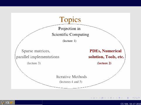
Outline
Part IPartial Differential Equations
Part IIMesh Generation and Load Balancing
Part IIITools for Numerical Solution of PDEs
CS 594, 03-17-2010
Part I
Partial Differential Equations
CS 594, 03-17-2010
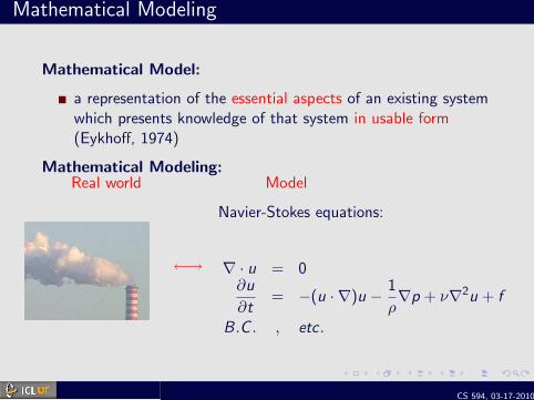
Mathematical Modeling
Mathematical Model:
a representation of the essential aspects of an existing systemwhich presents knowledge of that system in usable form(Eykhoff, 1974)
Mathematical Modeling:Real world Model
←→
Navier-Stokes equations:
∇ · u = 0∂u
∂t= −(u · ∇)u − 1
ρ∇p + ν∇2u + f
B.C . , etc .
CS 594, 03-17-2010
Mathematical Modeling
We are interested in models that are
Dynamici.e. account for changes in time
Heterogeneousi.e. account for heterogeneous systems
Typically represented with
Partial Differential Equations
CS 594, 03-17-2010
Mathematical Modeling
How can we model for e.g. Heat Transfer?
Heat* a form of energy (thermal)
Heat Conduction* transfer of thermal energy from a region of higher
temperature to a region of lower temperature
Some notations
Q : amount of heatk : material conductivityT : temperatureA : area of cross-section
CS 594, 03-17-2010
Heat Transfer
The Law of Heat Conduction
4Q
4t= k A
4T
4x
Change of heat is proportional to the gradient of the temperatureand the area A of the cross-section.
Q : amount of heatk : material conductivityT : temperatureA : area of cross-section
CS 594, 03-17-2010
Heat Transfer
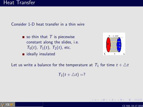
Consider 1-D heat transfer in a thin wire
so thin that T is piecewiseconstant along the slides, i.e.T0(t), T1(t), T2(t), etc.
ideally insulated
Let us write a balance for the temperature at T1 for time t +4t
T1(t +4t) =?
CS 594, 03-17-2010
Heat Transfer
T1(t +4t) ≈ T1(t)
+ k4t(T2(t)− T1(t))
(4x)2
+ k4t(T0(t)− T1(t))
(4x)2
= T1(t) + k4tT2(t)− 2T1(t) + T0(t)
(4x)2
Take lim4x ,4t→0
⇒ ∂T
∂t= k
∂2T
∂x2(Exercise)
CS 594, 03-17-2010
Heat Transfer
Extend to 2-D and put a source term f to easily get
∂T
∂t= k
(∂2T
∂x2+∂2T
∂y2
)+ f ≡ k 4T + f
Known as the Heat equation
CS 594, 03-17-2010
Other Important PDEs
Poisson equation (elliptic)
4u = f
Heat equation (parabolic)
∂T
∂t= k 4T + f
Wave equation (hyperbolic)
1
ν2
∂2u
∂t2= 4u + f
CS 594, 03-17-2010
Classification of PDEs
For a general second-order PDE in 2 variables:
Auxx + Buxy + Cuyy + · · · = 0
Elliptic:
if B2 − 4AC < 0
process in equilibrium (no time dependence)
easy to discretize but challenging to solve
Parabolic:
if B2 − 4AC = 0
processes evolving toward steady state
Hyperbolic:
if B2 − 4AC > 0
not evolving toward steady state
difficult to discretize (support discontinuoities) but easy tosolve in characteristic form
CS 594, 03-17-2010
How do we solve them?
Numerical solution approaches:
Finite difference method
Finite element method
Finite volume method
Boundary element method
CS 594, 03-17-2010
Finite Difference Method
use finite differences to approximate differential operators
one of the simplest and extensively used method in solvingPDEs
the error, called truncation error, is due to finiteapproximation of the Taylor series of the differential operator
CS 594, 03-17-2010
A Finite Difference Method Example
Consider the 2-D Poisson equation:
∂2u
∂x2+∂2u
∂y2= f
The idea, first in 1-D:
Use Taylor series to approximate d2udx2 (x) with
u(x), u(x + h), u(x − h)
u(x + h) = u(x) + hdu
dx(x) +
h2
2
d2u
dx2(x) +
h3
3!
d3u
dx3(x) +O(h4)
u(x − h) = u(x)− hdu
dx(x) +
h2
2
d2u
dx2(x)−
h3
3!
d3u
dx3(x) +O(h4)
⇒d2u
dx2(x) =
1
h2(u(x + h) + u(x − h)− 2u(x)) +O(h2)
CS 594, 03-17-2010
A Finite Difference Method Example
Similarly in 2-D
Use Taylor series to approximate 4u(x , y) withu(x , y), u(x + h, y), u(x − h, y), u(x , y + h), u(x , y − h).