Do Large AgglomerationsLead to EconomicGrowth? Evidence fromUrban India

Sabyasachi Tripathi

ISBN 978-81-7791-148-0

© 2012, Copyright ReservedThe Institute for Social and Economic Change,Bangalore

Institute for Social and Economic Change (ISEC) is engaged in interdisciplinary researchin analytical and applied areas of the social sciences, encompassing diverse aspects ofdevelopment. ISEC works with central, state and local governments as well as internationalagencies by undertaking systematic studies of resource potential, identifying factorsinfluencing growth and examining measures for reducing poverty. The thrust areas ofresearch include state and local economic policies, issues relating to sociological anddemographic transition, environmental issues and fiscal, administrative and politicaldecentralization and governance. It pursues fruitful contacts with other institutions andscholars devoted to social science research through collaborative research programmes,seminars, etc.

The Working Paper Series provides an opportunity for ISEC faculty, visiting fellows andPhD scholars to discuss their ideas and research work before publication and to getfeedback from their peer group. Papers selected for publication in the series presentempirical analyses and generally deal with wider issues of public policy at a sectoral,regional or national level. These working papers undergo review but typically do notpresent final research results, and constitute works in progress.

1

DO LARGE AGGLOMERATIONS LEAD TO ECONOMIC GROWTH?

EVIDENCE FROM URBAN INDIA

Sabyasachi Tripathi∗

Abstract

The cities and towns of India constitute the world’s second largest urban system besides contributing over 50 per cent of the country’s Gross Domestic Product (GDP). This phenomenon has been neglected by the existing studies and writings on urban India. By considering 59 large cities in India and employing new economic geography models, this paper investigates the relevant state- and city -specific determinants of urban agglomeration. In addition, the spatial interactions between cities and the effect of urban agglomeration on India’s urban economic growth are estimated. The empirical results show that agglomeration economies are policy-induced as well as market-determined and offer evidence of the strong positive effect of agglomeration on urban economic growth and support for the non-linearity of the Core-Periphery (CP) model in India’s urban system. Key Words: Urban Agglomeration, Urban Economic Growth, New Economic Geography, India. JEL Classification: O18, R11, R12

1. Introduction

In the past large cities were found mainly in the industrialized nations. However, today many of the

world’s largest cities are found in the developing countries. As per World Urbanization Prospects: 2009

Revision, the number of cities with population in excess of one million in the United States of America

(or India) was 12 (or 5) in 1950. It increased to 42 (or 46) in 2010 and was projected to reach 48 (or

59) by 2025. In an attempt to find the relevant factors responsible for the concentration of economic

activities in cities, the link between urban agglomeration and urban economic growth was studied by

Krugman (1991) and Fujita et al. (1999). It was done within the framework of New Economic

Geography (NEG) with the productivity differential leading to a shift of resources from agriculture or

hinterland region to an urban sector or core region. Compared to earlier location theories, a general

equilibrium framework with imperfect competition is new in NEG.

∗ PhD scholar in Economics at Centre for Economics Studies and Policy, Institute for Social and Economic Change,

Bangalore-560072, India; email: sabya.tripathi@gmail.com.

This paper is a part of my Doctoral Dissertation. I would like to thank my PhD supervisor Prof M R Narayana.

Without his constant guidance and inspiration, it would not have been possible for me to write this paper. I thank

Prof Meenakshi Rajeev, Dr Veerashekharappa, Dr Krishna Raj, Dr Elumalai Kannan, Dr Bibhu Prasad Nayak, Ms B P

Vani, Dr Laurent Bach, Dr Arne Melchior, Dr Gilles Duranton, Dr Jagannath Mallick, Dr Kala Seetharam Sridhar, Dr

Lengyel Balázs and Dr N R B Murthy for their very helpful comments and discussions. I am also grateful to the

DIMETIC Programme organiser for sponsoring my participation and giving me the opportunity to discuss my

research work in the DIMETIC Pecs 2010 and DIMETIC Maastricht 2010 sessions which helped me immensely in

understanding the New Economic Geography models and subsequently in producing this paper. However, the

usual disclaimer applies.

2

The population size and the number of urban centres in India are growing rapidly even as their

geographical boundaries are expanding. In this context, as Narayana (2009) points out, there is a

growing concentration of urban population in metropolitan areas (cities with a million-plus population)

compared to non-metropolitan areas in India. The growth in population is attributable to various factors

such as natural growth, rural-to-urban migration, expansion of city boundaries and reclassification of

rural areas as urban. At the beginning of the Twentieth Century, for instance, there was only one city

with a population of more than a million, namely, Kolkata (then known as Calcutta with a population of

1.5 million). In 1991, there were 23 cities with million-plus population accounting for about 33 per cent

of the total urban population. However, by 2001, the number of million-plus cities increased to 35

(supporting about 38 per cent of the total urban population). Further, in 2001, there were six mega

cities (with population over five million) in India, namely, Kolkata, Mumbai, Delhi, Chennai, Bangalore

and Hyderabad.

The Indian urban economy too is growing and making a sizeable contribution to the country’s

national income. For instance, the share of urban economy in the total net domestic product (NDP)

increased from 37.65 per cent in 1970-71 to 52.02 per cent in 2004-05 and accounted for about 6.2 per

cent growth rate of urban NDP from 1970-71 to 2004-05 at constant prices (1999-00). Within urban

NDP, the share of the industrial and service sectors was about 27 per cent and 72 per cent respectively

in 2004-05 at constant (1999-00) prices.

The major explanation of urban agglomeration and its effect on economic growth has been

studied in the NEG theory since the pioneering work of Krugman (1991). The NEG models involve a

tension between the “centripetal” forces (pure external economics, variety of market scale effects and

knowledge spillovers) that tend to pull population and the production process towards agglomerations

and the “centrifugal” forces (congestion and pollution, urban land rents, higher transportation costs and

competition) that tend to break up such agglomerations (Overman and Ioannides 2001, Tabuchi 1998).

While formalizing the interplay of agglomeration and dispersion forces, the CP model explains the

formation of dynamic urban system and finds a “ ”-shaped curve between the distance of a regional

center and a local market potential in a single-core urban system (Partridge et al 2009, Fujita et al

1999). This curve shows that as the relative distance to a central city increases, the market potential

declines first, later rises and then declines again. But CP models mostly remain difficult to manipulate

analytically making the model consistent with data as most of the results derived in the literature are

based on numerical simulation (Fujita and Mori 1997, Fujita et al 1999a) and the nonlinear nature of

geographical phenomena (Fujita and Krugman 2004).

Black and Henderson’s (1999) studies established that that population growth was faster in

cities that are closer to a coast and cities with bigger initial populations, though this effect weakens as

neighbouring population masses become larger. Dobkins and Ioannides (2000), Ioannides and Overman

(2004), using the US metropolitan data for 1900-1990, provide evidence that the distance from the

nearest higher-tier city is not always a significant determinant of size and growth and that there is no

evidence of persistent non-linear effects of either size or distance on urban growth. Chen et al (2011)

estimate the impact of spatial interactions in China’s urban system on urban economic growth over the

3

period 1990-2006. Their results verify the non-linearity of the CP Model of urban system and find

presence of agglomeration shadow in Chinese urban economies.

In the context of identifying relevant factors behind urban agglomeration, Da Mata et al (2005)

observe that increases in rural population supply, improvements in inter-regional transport connectivity

and educational attainment of the labour force have a strong impact on city growth in Brazil. Ades and

Glaeser (1995) find that, as predicted by Krugman and Elizondo (1996), countries with high shares of

trade in GDP or low tariff barriers (even holding trade levels constant), rarely have population

concentrated in a single city, but remain skeptical as to the existence of a direct casual link. The cross-

country analysis shows the negative impact of the development of transportation networks and the

positive impact of capital city dummy, non-urbanized population of a country, urbanized population

outside the main city, real GDP per capita, share of the labour force outside of agriculture and the

concentration of power in the hands of a small cadre of agents living in the capital city of a country.

This is positively related to urban primacy in the main city of a country. Henderson (1986), Wheaton

and Shishido (1981) show that across a small sample of countries, increased government expenditure,

including non-federalist governments, leads to urban concentration. Further, Henderson (2010) finds

that the level of urbanization and income per capita are highly correlated [R2 =0.57].

Many studies have found a link between urban agglomeration and economic growth. Brülhart

and Sbergami (2009) found that the agglomeration process boosted the growth of GDP only up to a

certain level of economic development. Fujita and Thisse (2002) found that “growth and agglomeration

go hand-in-hand,” whereas a review paper by Baldwin and Martin (2004) emphasized on the result that

given localized spillovers “spatial agglomeration is conducive to growth”. Ades and Glaeser (1995)

examined economic growth across a cross-section of American cities and found that income and

population growth moved together and the growth of both were positively related. Henderson (2003)

found that urban primacy (the share of a country’s largest city) was advantageous to growth in low-

income countries. On the other hand, Au and Henderson (2006) estimated the net urban agglomeration

economies for Chinese cities and found that current government policy for city population

agglomeration is bad for the country. Wheaton and Shishido (1981) and Rosen and Resnick (1980)

observed that urban concentration first increased and then decreased in respect of a country’s per

capita GDP. In the case of developing countries, Henderson (2005) also found a positive effect of urban

agglomeration on city productivity and growth.

Among the Indian studies, Sridhar (2010) estimated the determinants of city growth and

output both at the district and city levels and found that factors like proximity to a large city and the

process of moving from agriculture to manufacturing determines the size of a city. In 1986, Mills and

Becker used a national sample of large Indian cities and then a sample of cities in the large Indian state

of Madhya Pradesh to establish that a large initial population discouraged further growth of cities with

an initial population below one million. They also found that cities grew faster in higher income states

than in lower income states. Finally, they argued that the farther the cities are from the nearest Class I

city (with a population of more than 100,000), the faster they grow. The study by Narayana (2009)

showed the dispersion of metropolitan population though there is growing concentration of urban

population in metropolitan areas compared to non-metropolitan areas. Furthermore, some studies on

4

India (Lall and Mengistae 2005, Lall and Rodrigo 2001, Lall et al 2004, Chakravorty and Lall 2007) focus

on industrialization-related urban agglomeration and urban economic development through the

framework of NEG models.

Given the above review of studies, the determinants of urban agglomeration and its impact on

urban economic growth and empirical research on “non-linearity” of CP model to explain the urban

system are the key researchable issues in the Indian context. These issues form the key focus and

objective of this paper. To our knowledge, this paper is a beginning to analyze the impact of urban

agglomeration on India’s urban economic growth using the sub-national (i.e., state and urban) level

data.

The paper is organized as follows. In the next section, we explain the model and its

econometric specification for the empirical analysis. Sections 3 and 4 outline the measurement of

variables with data sources and a short description of the data used for the analysis, respectively.

Section 5 highlights the details of estimated results followed by a summary of major conclusions and

implications in Section 6.

2. Empirical Framework

For the empirical analysis of the determinants of urban agglomeration and spatial interaction among

cities on economic growth, we employ the commonly used reduced form estimation procedure (Dobkins

and Ioannides 2000, Brülhart and Koenig 2006). Based on the economic growth model of Barro (2000),

the cross-section OLS regression method is used as the basic reduced-form CP model for measuring

India’s urban economic growth. The potential endogeneity problem of OLS estimation is not a main

concern here as all the explanatory variables are either exogenous geographic factors or initial values of

those control variables. To estimate the relevant state- and city-specific determinants of urban

agglomeration and its effect on urban economic growth, the following multiple regression OLS

technique in the form of recursive econometric model is used.

2.1. Recursive equation model

The basic model for estimation of the determinants of urban agglomeration is stated as follows:

UA = α0 + α1X 1 + α2X2 + α3X3 + α4X4 + α5X 5 + α6X6 + α7X7 + α8X8 + α9X 9 +

α10X 10 + α11X11 + α12X 12 + u1 ------------------------------------------ (1)

where UA stands for population of urban agglomeration, X1 refers to market size effect, X2 for distance

from a bigger city, X3 for degree of state trade openness, X4 refers to transportation cost, X5 for city

vehicle density, X6 refers to city proximity to natural ways of communication, X7 for environmental

effect, X8 refers to size of a state, X9 for state industrial development, X10 refers to state urbanization

level, X11 for political power and political stability and X12 refers to government policy for urban

agglomeration. Equation (1) is a linear regression model and estimated by OLS. The stochastic error

term u1 satisfies the Classical Linear Regression Model (CLRM) assumptions. Predicted signs of the

5

coefficients are the following: α1>0, α2<0, α3<0, α4<0, α5<0, α6>0, α7>0, α8<0, α9>0, α10>0, α11>0,

and α12>0.

To capture the positive effect of First Nature Geography (FNG) on urban agglomeration, we

consider the following two variables: 1) city environmental effect because it may have positive

influence on the concentration of population in a large city by way of encouraging in-migration of

population with favourable climatic conditions (Sridhar 2010). 2) The proximity to natural ways of

communication because it encourages development of the large hubs of international trade by

absorbing the potential initial advantages of the benefits from easy access to international and domestic

market [Krugman 1993].

NEG models [mainly Second Nature Geography (SNG)] explain urban agglomeration by

considering the relevant positive and negative factors. Positive factors include the size of the market

because a bigger market encourages firms to produce a wider variety of goods (due to advantage of

increasing returns at firm level and pooled labour market) that can be consumed by the city dwellers.

On the other hand, negative factors include the following variables: First, distance from a bigger city

because bigger cities become primary magnets of economic activity and longer distance to a bigger city

indicates lower market potential. Second: degree of state trade openness because when a country

trades less with rest of the world the domestic transaction becomes more important and these

transactions can in general be conducted more cheaply over shorter distances. This process is reversed

when more countries trade with the rest of the world (or have more liberalized trade norms), as

theoretically predicted by Krugman and Elizondo (1996) and elaborated by Brülhart and Sbergami

(2009). Third: high government expenditure on transportation because high internal transport costs

provide incentive for the concentration of economic activity (Ades and Glaeser 1995). Fourth: higher

vehicle density because it captures the external diseconomies.

Among the other variables, we expect the following to have a positive effect on large city

populations. The first is political power because proximity to power widens the scope of political

influence, encourages the government to transfer resources to the capital city and attract migrants in

the process. Furthermore, rent-seekers coming to the capital may also contribute to the growth of the

city’s population (Ades and Glaeser 1995). Second is the higher government expenditure on various

projects (or better quality of public services) because it attracts more workers and firms to the city.

Third is the industrial development (or economic development) because more workers are absorbed and

the production process is concentrated mainly in the large city. Fourth is the higher level of urbanization

of a state because it is associated with higher population concentration in a large city. On the other

hand, large city urban concentration declines with the increase in the state’s land area (or geographic

size) because we assume that there is a positive link between the bigger state size, dispersion of state

resources and formation of more cities (Henderson 2003). Finally, we predict that political instability has

a negative effect on agglomeration because it creates an unfriendly environment for the city dwellers.

Given the estimated model in (1) the following equation estimates the determinants of urban

economic growth:

? ? ? �?? ? ?? �? ?? ? ?? ? ? ? ?? ? ? ? ?? ? ? ? ?? ?? ? ?? ? ? ? 2u

------------------------------------ (2)

6

where UG stands for urban economic growth, ? ?? �refers to predicted values of the dependent variable

(i.e., urban agglomeration) of Equation (1), Z1 stands for city density (or growth rate of city density), Z2

refers to special interaction among cities, Z3 refers to size of a city, Z4 stands for effect of human capital

accumulation, and Z5 stands for initial level of per capita real city output. Equation (2) is a linear cross-

section regression model, which is estimated using OLS technique and u2 is a well-behaved error term.

Predicted sign of the coefficients are the following: β1>0, β2>0, β4>0,β5>0, and β6<0 (β6>0) if the

economy experiences (or does not experience) conditional convergence. However, following the

prediction of CP model, distance to a bigger city has a negative effect (i.e., βs<0) on city economic

growth whereas square and cubes of distances have positive (i.e., βs>0) and negative effects (i.e.,

βs<0).

Following the NEG models, we expect India’s large city urban agglomeration to have a strong

positive effect on urban economic growth because the bigger cities have higher productivity, wages and

capital per worker (i.e., higher economies of agglomeration) and bigger efficiency benefits (Duraton

2008) as empirically supported by the World Bank (2004) research work and elaborated in Narayana’s

(2009) study. In addition, major factors behind the existence of urban increasing returns, include

sharing (e.g., local infrastructure), matching (e.g., employers and employees), and learning (e.g., new

technologies) (Duraton and Puga 2004).

Among the other factors we expect distance to large city to have a negative effect on city

economic growth and squares and cubes of distances have positive and negative effects, respectively,

as the CP model of NEG theory (Fujita et al 1999) shows that with the distance to a large city

increasing, the market potential declines first, and later rises, then declines again. The theory finds the “

”- shaped correlation between distance to a large city and economic activities. Further, education

(capture the initial economic growth effect) has a positive effect on city’s economic growth (Barro

2000), as the accumulation of human capital can create a pool of skilled labour force by attracting firms

and residents. Following economic growth literature, we also expect initial income to have an effect on

the conditional convergence of the city’s income growth rate. Finally, economic growth may benefit

from the size of the city so we expect a positive effect of higher urban economic growth in larger cities.

Equations (1) and (2) together constitute the recursive equation system for estimation of determinants

of large city agglomeration and its impact on urban economic growth.

3. Measurement of variables and data sources

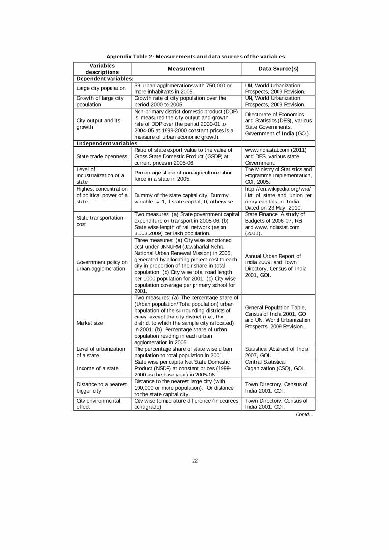
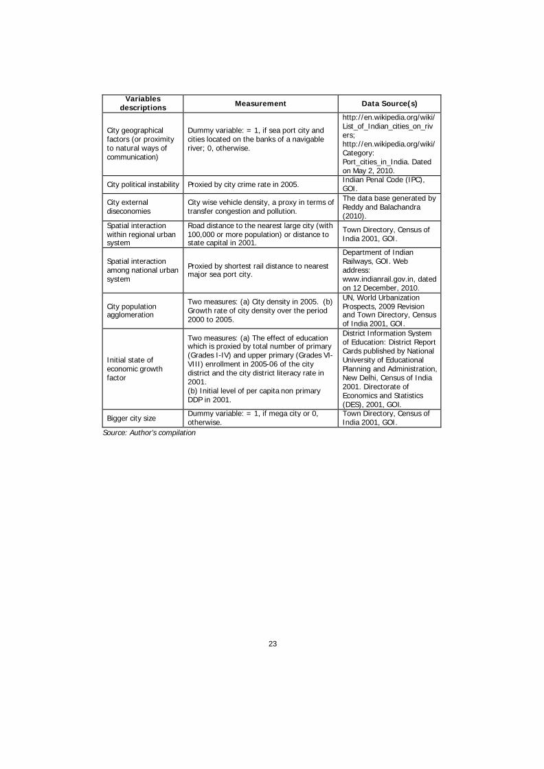
Appendix Table 1 presents the name of the cities used in the analysis. Appendix Table 2 summarizes

the descriptions, measurements, and data sources of all the variables used in the estimation of

recursive econometric model of Equations (1) and (2).

4. Description of data

Appendix Table 3 gives the means, standard deviations, minimum, and maximum values for the

variables that we use in our regression estimations. Most importantly, standard deviations (measures

the variability of the variables) are found higher for state government expenditure on transport, city

7

wise sanctioned cost under JNNURM and total number of primary and upper primary district enrollment,

which indicate that the data points for these variables are spread out over a large range of values.

Appendix Tables 4 and 5 show the raw correlation of the variables. In Appendix Table 4, the

values of the correlation coefficient (r2) show that large city population is positively associated with the

percentage of urban population residing in each urban agglomeration (i.e., r2 is 0.92), sanctioned cost

under JNNURM (i.e., r2 is 0.71), population coverage per primary school (i.e., r2 is 0.49), and state-level

urban population (i.e., r2 is 0.42). On the other hand, large city population agglomeration is negatively

correlated with distance to state capital city (i.e., r2 is 0.34), city wise total road length per 1,000

population (i.e., r2 is 0.26), and distance to large city (i.e., r2 is 0.18). Moreover, Appendix Table 5

shows that the city output growth rate is positively associated with total number of primary and upper

primary enrollment, district literacy rate, initial level of per capita DDP, and growth rate of city density.

In contrast, city output growth rate is negatively correlated with distance to large city, distance state

capital city, and distance to sea port city. Due to existence of multicollinearity problem in the raw data,

we considered the following two remedies: First, we chose an appropriate model specification by

dropping the high collinear variables. Second, we transformed the equation in to its logarithmic form.

Key proxy variables in the estimation include the following: (a) City district literacy rate to

capture the human capital accumulation, as literate people generally have a higher socio-economic

status by enjoying better health status and employment prospects. (b) Total number of primary and

upper primary enrollment as a second proxy variable of human capital accumulation, because high rate

of enrollment in school made faster growth in per capita income through rapid improvement in

productivity (Bils and Klenow 2000). (c) Driving (or road/railway) distance is used for approximating the

spatial interactions between cities as in Hanson (1998 and 2005). (d) Non-primary DDP as a proxy of

city output because NEG theories emphasize the agglomeration of manufacture and service sectors

(Krugman 1991 and used in Sridhar 2010 for Indian case).1 (e) Due to lack of estimates of GSDP at

market prices, GSDP at factor cost in current prices is used. (f) Crime rate is used as a proxy for political

instability as it indicates the law and order situation in a state. (g) State-wise length of rail network per

lakh population is used as a proxy for state transportation cost because it measures the internal

transport costs (Krugman 1991). (h) Temperature differences are used as a proxy for environmental

effect as in Haurin (1980) and Sridhar (2010). (i) Population coverage per primary school and total road

length per 1,000 population are used as proxies for government expenditure for urban agglomeration,

following the certain studies (Sridhar, 2010). (j) Percentage of population living in each urban

agglomeration and percentage share of district urban population of surrounding city districts are used

as proxies for city market size because they show higher percentage with higher population in the main

city. (k) Vehicle density is used as a proxy for congestion because it contributes to low density

development and often reduces transit use. (f) Population size is used as a measure of urban size as it

captures both geographical and economic size of urban areas (Narayana 2009).

8

5. Results of estimation

5.1. Determinants of urban agglomeration

Table 1 presents the results of size models of the determinants of urban agglomeration based on

Equation (1) by employing the OLS method. Log of city population and growth rate of city population

are used as dependent variables in the estimation. The models which are estimated are not only

different in specifications but also by number of observations. Regression (1) shows the estimates of

the full model which includes all variables for maximum number of available observations. Regression

(2) to (6) report results for a parsimonious model, excluding controls that are not found to be

statistically significant or matched with the expected sign of the regression parameters. More

specifically, due to paucity of data, we ran Regressions (2) to (6) and have presented the results of the

best fitted models in terms of predicted signs, significance level of the variables and goodness of fit of

the regressions, according to available different number of observations of the variables. All the

regressions report OLS results with robust standard errors (to correct heteroskedasticity) in parentheses

with taking care (or absence) of multicollinearity problem.

Regression (2) includes the set of controls of the best fitted model for maximum number of

available observations. The regression explains 88 per cent of the total variation in the dependent

variable. In Regression (2), among the proxy variables of government policy for urban agglomeration,

we find that city cost sectioned under JNNURM has a positive and statistically significant effect on urban

agglomeration which is line with our working hypothesis. In particular, a 10 per cent increase in

expenditure through JNNURM is associated with 1.4 per cent increase in large city population and

supports the positive effect of government policy on urban agglomeration. In contrast, the second proxy

variable (or city wise total road length per 1,000 population) for measuring the government policy for

urban agglomeration does not show the expected relationship. In addition, we find that the coefficient

of state capital dummy is positive but not significant.

The results also show that the percentage of urban population residing in each urban

agglomeration (market control variable) is positive and significant. The findings support our expected

hypothesis and show that a 10 per cent increase in urban population residing in each urban

agglomeration increases concentration of large city population by 4.7 per cent. On the other hand, the

percentage of district urban population in the surrounding city districts (which shows higher percentage

with higher population of the main city) explains the negative and significant effect (at 5 per cent level)

on large city population agglomeration. The result runs counter to the expected hypothesis and

indicates that over-concentration of city population has a negative effect on further urban

agglomeration.

The estimated coefficient of the state trade openness variable is positively and significantly

related to the large city population agglomeration, which runs against the predicted hypothesis. An

increase of 10 per cent in the share of trade in GSDP leads to 9.3 per cent increase in the population

agglomeration. This finding concludes that the degree of state trade liberalization is not enough to curb

the population agglomeration of the large city. The results also show that the distance to a large city (or

distance to state capital city) has a negative (as predicted) and insignificant effect on city population

concentration. Among the three variables used to capture the role of FNG for explaining urban

9

agglomeration, dummy of cities located on river banks has a positive (expected) and significant (at 1

per cent level) effect on urban agglomeration. The coefficient of sea port city dummy has a positive and

statistically insignificant impact on the concentration of city population.

The coefficient of temperature differences shows a positive value which implies that extreme

weather conditions encourage urban agglomeration. However, the relationship between temperature

differences and urban agglomeration does not seem to be stronger as the coefficient is not statistically

significant. The finding suggests that temperature differences (as expected impact was negative) do not

play an important role in explaining India’s urban agglomeration.

Regression (3) reports estimates with a parsimonious set of controls. As usual, the cross

section agglomeration regression performs well, explaining up to 79 per cent of sample variance in the

population agglomeration of the large cities. The state-level urbanization variable (state-wise

percentage of urban population) is positive and significant at 5 per cent. The coefficient 0.013 indicates

that with a 10 per cent increase in state urban population, large city population increases by 0.1 per

cent. This result suggests that higher level of state urbanization mainly depends on the concentration of

population in the large cities. We also find a negative and significant effect (as expected) of state land

area (state size) on concentration of city population. The value of the coefficient suggests that with a 10

per cent increase in size of the state, city population agglomeration decreases by 1.7 per cent. The

regression results show that, as expected, state-wise percentage of workers in non-agriculture has a

positive and significant effect on population agglomeration. On the other hand, transport cost control

variable and state government capital expenditure on transport (or state- wise length of rail network)

takes on negative coefficients that are in line with our working hypothesis. However, surprisingly both

the coefficients in Regression (3) are not statistically significant. The results also report that the

significance level of city sanctioned cost under JNNURM (or dummy of the cities located in the bank of

river) improved from 10 per cent (or 5 per cent) in Regression (2) to 1 per cent in

10

Table 1: Economic Determinants of large city population agglomeration: Estimates of log

linear regression model

Dependent variables:

Log of large city population in 2005 Growth

rate of city population

(1) (2) (3) (4) (5) (6)

Intercept 8.80*** (2.84)

6.92*** (0.237)

7.48*** (1.22)

10.19*** (1.39)

-0.236 ( 2.59)

0.037** (0.017)

Distance to state capital city

-0.035 (0.038)

-0.024 (0.032)

-0.034 (0.039)

-0.001** (0.0005)

-0.001** (0.0004)

Share of trade in GSDP 0.916 (1.07)

0.929* (0.551)

3.24*** (0.666)

2.41** (0.811)

0.03 (0.021)

City-wise sanctioned cost under JNNURM

0.138 (0.095)

0.143* (0.085)

0.445*** (0.077)

-0.001 (0.002)

Distance to large city 0.001 (1.19)

-0.017 (0.106)

-0.006*** (0.002)

-0.006*** (0.002)

State capital dummy 0.018 (0.152)

0.025 (0.139)

0.718*** (0.234)

0.579** (0.235)

0.004 (0.003)

City-wise total road length per 1000 population

-0.049 (0.068)

-0.049 (0.069)

-0.086 (0.078)

-0.3*** (0.086)

-0.002** (0.001)

State-wise percentage of workers in non-agriculture

-0.007 (0.009)

0.014* (0.008)

0.036*** (0.012)

Log of population coverage per primary school

-0.079 (0.085)

-0.163 (0.13)

-0.177* (0.096)

-0.061 (0.224)

Dummy of the cities located in bank of river

0.202 (0.125)

0.234** (0.112)

0.398*** (0.129)

0.002 (0.003)

percentage of state- level urban population

0.001 (0.009)

0.013** (0.006)

-0.015* (0.009)

State govt. capital expenditure on transport

0.03 (0.067)

-0.041 (0.062)

-0.049 (0.072)

-0.001 (0.001)

Sea port city dummy 0.092

(0.229) 0.105

(0.226) 0.229

(0.183) 0.001

(0.004) Parentage share of district urban population of surrounding city district

-0.011* (0.005)

-0.009** (0.004)

Log of per capita real NSDP -0.039 (0.216)

0.719*** (0.182)

Percentage of urban population residing in each urban agglomeration

0.499*** (0.047)

0.477*** (0.041)

Log of state land area -0.023 (0.086)

-0.167* (0.083)

City temperature differences

0.005 (0.004)

0.003 (0.004)

-0.003 (0.012)

State-wise rail network per lakh population

-0.012 (0.028)

-0.123** (0.046)

City crime rate -0.024 (0.043)

-0.007 (0.035)

City vehicle density (VD) -0.002** (0.0008)

No. of Observation 59 59 58 34 23 52 R2 0.89 0.88 0.79 0.86 0.90 0.16 �? ? 0.85 0.86 0.76 0.79 0.84 -0.03 Note: Figures in parentheses represent robust standard errors. ***, ** and * indicate statistical

significance at 1%, 5%, and 10% level, respectively. Source: Estimated using equation (1).

11

Regression (3). However, the coefficient of the distance to state capital city (or city-wise road

length per 1,000 population) again remains statistically insignificant. In Regression (4), we add city

crime rate (capture the city political instability) and third proxy measurement of government policy for

urban agglomeration (i.e., log of population coverage per primary school) to our earlier regression. Both

the coefficients of the variables are negative which match with the expected sign condition, even

though, the result is not significant. On the other hand, the positive and statistically significant

coefficient of state capital dummy indicates that large cities are 72 per cent larger if they also happen to

be state capital cities. This may mean that power attracts population or indicate that state capitals are

located in larger cities. The variance inflation factor (VIF) test indicates that result does not suffer from

any multicollinearity effect as the VIF value for state capital dummy is 3.48 in this context. Distance to

large city (or distance to state capital city) has a negative (as predicted) and significant effect on

concentration of city population and indicates that proximity to large cities makes cities larger as well,

implying the existence of market and scale economies. The VIF value is 1.52 (or 2.65) for the coefficient

of distance to large city (or distance to state capital city) which indicates no problem of multicollinearity.

However, the significant and negative sign of city-wise total road length per 1,000 population coefficient

does not show the expected relationship as it runs against our expected sign. The VIF value for this

coefficient is 2.20 suggesting free of any multicollinearity effect. The coefficient of state wise length of

rail network is negative and significant which implies that with a 10 per cent increase in state wise

length of rail network the concentration of population in a large city decreases by almost 1.2 per cent.

The VIF value for the coefficient of state wise length of rail network is 2.28. Moreover, the results also

show that significance level of the state trade openness variable increased from 10 per cent in

Regression (2) to 1 per cent in this regression. The VIF value (i.e., 2.50) of the coefficient of state trade

openness variable does not show any multicollinearity effect.

In contrast, the coefficient of the state government capital expenditure on transport (or sea

port city dummy) does not show any improvement from the earlier regression results in terms of level

of significance. Regression (5) includes a state-level industrial proxy variable: state per capita income.

The positive and significant coefficient of state per capita income variable indicates that the level of

industrial development of a state increases the population agglomeration of a large city. A 10 per cent

increase in state per capita income increases large city population by 7.2 per cent. As expected, the

coefficient of city vehicle density (control for city external diseconomies) is negative and significant at 5

per cent. This implies that higher congestion and pollution lead to lower urban agglomeration. The

positive and significant (at 1 per cent) coefficient of the state share of workers engaged in all non-

agricultural activity (capture the proportion of population that is not conditioned to natural resources)

implies that the large cities require some economic development through industrialization. On the other

hand, public services such as population coverage per primary school show a negative and significant

relationship implying that population coverage by primary schools (a large number of persons per

school) discourages cities from becoming larger. The result strongly suggests that India’s agglomeration

economies are policy induced. The estimates of Regression (5) also provide consistent results for the

other variables that include distance to state capital city and distance to large city, as the coefficients of

these variables are significant and go with our expected signs. However, the coefficients of share of

12

trade in GSDP and state capital city dummy lose significance level from 10 per cent to 5 per cent from

Regression (4). In addition, again the coefficient of city crime rate shows the negative and an

insignificant effect on urban agglomeration.

In Regression (6), city population growth rate has been used as a proxy for urban

agglomeration because this specification gives us the best fitted predicted values of the dependent

variable which is used as an independent variable in Equation (2) for capturing the positive effect of

urban agglomeration on urban economic growth endogenously, suggesting that the changes in level of

agglomeration directly effect on the changes of urban economic growth.2 The Regression (6) explains

only 16 per cent of the total variation in the dependent variable. The results show that the level of state

urbanization (or city-wise total road length per 1,000 population) has a negative and significant effect

on city population growth. The coefficient indicates that a 10 per cent increase in state level

urbanization (or city-wise total road length per 1,000 population) is associated with a reduction of 0.2

(or 0.02) per cent in large city population growth rate. We also find that state trade openness, state

capital dummy, dummy of the cities located in bank of river and sea port city dummy have a positive

(as expected) effect on growth rate of city population. However, surprisingly none of the variables is

found to be statistically significant. In addition, the coefficients of the population coverage per primary

school, city wise temperature differences, and state government expenditure on transport show the

negative and insignificant effect on growth rate of city population.

5.2. Determinants of urban economic growth

In Regression (7), we present the results with controlling entire variables along with agglomeration

variable (predicted values of agglomeration variable of Regression (6) used in Equation (2). Though we

find agglomeration effect has a positive and significant effect on city economic growth but most of the

other variables do not match with our expected sign and show the lower level of significant (or

insignificant) effect.

Therefore, we run Regressions (8) to (12) excluding controls that are not plausible in terms of

expected signs and level of significance of the variables. In Regression (8), we only measure the effect

of agglomeration on urban economic growth without controlling any other variables, while in Regression

(9) we capture the effects of linear form of distance variables on urban economic growth. Finally, we

run Regressions (10) to (12) separately for three proxy measurements of the distance variable in the

form, which is predicted in the CP model of NEG theory. As the raw data shows that prominently a “

”-shaped curve relationship exists between the distance to the state capital city and distance to large

city with urban economic growth, we add square and cube terms in Regressions (11) and (12) for these

two distance variables, respectively. In contrary, the raw data does not show any strong nonlinear

relationship between distance to a sea port city and urban economic growth. Therefore, we consider

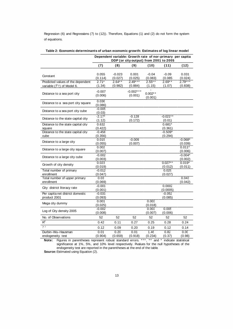
only linear term of this distance variable in Regression (10). Table 2 summarizes the estimates of the

Regressions from (7) to (12) based on Equation (2). We also perform Durbin–Wu–Hausman

endogeneity test the potential endogeneity problem. However, the large p-values for Regressions (7) to

(12) indicate that OLS is consistent. In addition, Regressions (7) to (12) are estimated separately, as we

did not find any positive contemporaneous correlation (i.e., correlation between error terms of

13

Regression (6) and Regressions (7) to (12)). Therefore, Equations (1) and (2) do not form the system

of equations.

Table 2: Economic determinants of urban economic growth: Estimates of log linear model

Dependent variable: Growth rate of non-primary per capita

DDP (or city output) from 2001 to 2005

(7) (8) (9) (10) (11) (12)

Constant

0.055

(0.114)

-0.023 (0.027)

0.001

(0.025)

-0.04

(0.083)

-0.09 (0.085

0.031

(0.024) Predicted values of the dependent variable (? ?? ) of Model 6.

2.71* (1.34)

2.64** (0.982)

2.49*** (0.884)

2.55** (1.15)

2.69** (1.07)

2.79*** (0.838)

Distance to a sea port city -0.007 (0.006)

-0.002*** (0.001)

-0.002** (0.001)

Distance to a sea port city square 0.036 (0.086)

Distance to a sea port city cube -0.005 (0.03)

Distance to the state capital city -2.17* (1.12)

-0.128 (0.172)

-0.021** (0.01)

Distance to the state capital city square

0.632 (0.422)

0.681* (0.361)

Distance to the state capital city cube

-0.456 (0.356)

-0.509* (0.294)

Distance to a large city 0.015

(0.055) -0.009 (0.007)

-0.068* (0.039)

Distance to a large city square 0.002

(0.007) 0.011* (0.006)

Distance to a large city cube -0.002 (0.003)

-0.004* (0.002)

Growth of city density 0.023 (0.019)

0.027** (0.012)

0.019* (0.011)

Total number of primary enrollment

-0.012 (0.047)

0.029 (0.027)

Total number of upper primary enrollment

0.03 (0.069)

0.043 (0.042)

City district literacy rate -0.001 (0.001)

0.0002 (0.0005)

Per capita net district domestic product 2001

-0.031 (0.093)

-0.052 (0.085)

Mega city dummy 0.001

(0.025) 0.003

(0.018)

Log of City density 2005 -0.002 (0.008)

0.003 (0.007)

0.005 (0.006)

No. of Observations 52 52 52 52 52 52

R2 0.42 0.11 0.27 0.25 0.28 0.24 �? ? 0.12 0.09 0.20 0.19 0.12 0.14 Durbin–Wu–Hausman endogeneity test

0.01 (0.904)

0.20 (0.659)

0.01 (0.918)

1.46 (0.234)

0.82 (0.37)

0.00 (0.98)

Note: Figures in parentheses represent robust standard errors. ***, ** and * indicate statistical significance at 1%, 5%, and 10% level respectively. P-values for the null hypotheses of the endogeneity test are reported in the parentheses at the end of the table.

Source: Estimated using Equation (2).

14

The result of Regression (8) shows that the agglomeration (controlled in endogenously)

variable has a positive and significant effect on urban economic growth. This positive impact of

agglomeration on growth matches with our main working hypothesis. In particular a 10 per cent

increase in urban agglomeration increases urban economic growth by 26 per cent. In Regression (9),

the coefficients of the linear item of distance to a large city, distance to state capital city and distance to

a major ports are negative, which implies that urban economic growth decreases away from a large city

(or state capital city) and major ports. However, the coefficient of distance from a major sea port city is

the only variable (among the three variables) which is significant at 1 per cent level. Results of the

Regression (10) show that the coefficient of distance to a sea port city is negative and statistically

significant which again indicates that urban economic growth decreases away from major ports. The

value of VIF 1.84 indicates there is no multicollinearity effect on the coefficient of distance to a sea port

city. In Regressions (11) and (12), the coefficients of the distance to the nearest large city (or state

capital city) and its square and cube are all significant and all present the expected signs which offer

evidence of the non-linearity pattern of India’s urban system.

Most importantly, the growth rate of city density (capture the internal population

agglomeration) has a positive and significant effect on urban economic growth. The result of

Regression (11) shows that a 10 per cent increase in growth of city density is associated with 0.3 per

cent increase in city output. The results clearly suggest that in India, large city urban agglomeration

(controlled endogenously or exogenously) leads to urban economic growth.3 However, the coefficient of

city density has a positive but insignificant effect on urban economic growth.

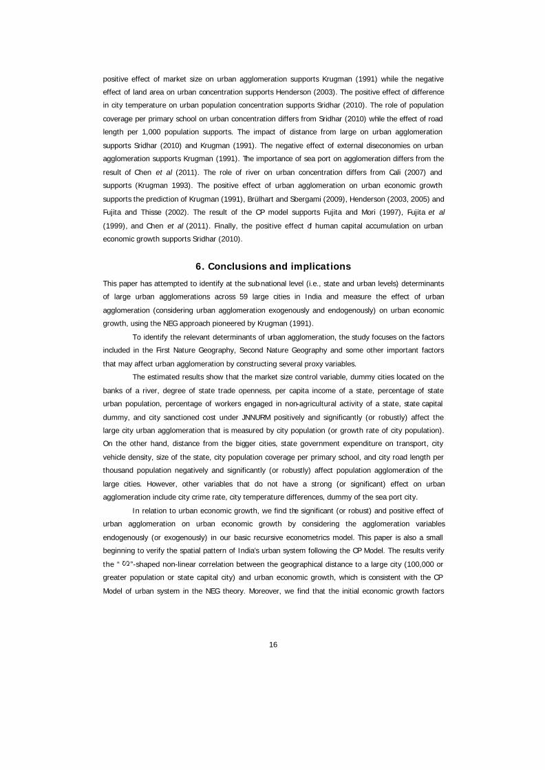
Based on the estimated results to approximate the exact distance in which urban economic

growth is positive (or negative) as predicted in the CP model, we simulate the correlation between

distances to large cities (or state capital cities) and urban economic growth. In Figures 1 and 2, the

horizontal axis represents the distance (kilometres) away from large cities (or state capital city), and the

vertical axis is the urban economic growth rate (percentage). Two figures show the CP pattern of India’s

urban system and support the theoretical prediction of NEG models.

-1.5

-1.3

-1.1

-0.9

-0.7

-0.5

0 50 100 150 200

Urb

an E

cono

mic

gro

wth

(%

)

Distance (Km.)

Fig.1. Distance to Large City andUrban Economic Growth

15

Source: Based on estimated results of regression (12) Source: Based on estimated results of

regression (11)

Figures 1 and 2 suggest that while a city is located away from a large city (or state capital

city), within 40 km (or 200 km) but closer to a large market, it has potential for higher economic growth

rate. When distance is long enough, more than 110 km from a large city (or 700 km from the state

capital city), the city suffers low market potential and poor economic growth rate.

Regression (11) suggests that the total number of primary enrollment (or city literacy rate) has

a positive effect on city economic growth. In addition, Regression (12) shows that the total number of

upper primary enrollment also has a positive effect on city economic growth. The results support the

prediction about the positive effect of human capital accumulation on city economic growth rate. But

the values of estimated coefficients are not significant. Regression (11) shows that the per capita net

non-primary DDP (controlled to observe whether the Indian economy is experiencing conditional

convergence at the city level) has an insignificant negative impact on India’s urban economic growth

and no significant change in conditional convergence. Regression (10) further examines the role of

bigger city size (i.e., over size of city captured by mega city dummy) on urban economic growth and

finds the insignificant positive effect of mega city dummy urban economic growth.

The positive effect of capital city, per capita GSDP and level of urbanization on urban

concentration support the findings of Ades and Glaeser (1995). The positive effect of government

expenditure through various projects on urban concentration supports the finding of Henderson (1986),

Wheaton and Shishido (1981). The positive effect of trade openness on urban concentration supports

Brülhart and Sbergami (2009), Duranton (2008) and Fujita and Mori (1996) and differs from Krugman

and Elizondo (1996). The negative effect of transport cost on urban agglomeration supports the findings

of Krugman (1991), Ades and Glaeser (1995). The positive effect of industrial development on

population concentration supports the finding of Murphy et al (1989), Ades and Glaeser (1995). The

-2.5-2

-1.5-1

-0.50

0.51

1.5

0 200 400 600 800 1000

Urb

an E

cono

mic

gG

owth

(%)

Distance (Km.)

Fig. 2. Distance to the State Capital and Urban Economic Growth

16

positive effect of market size on urban agglomeration supports Krugman (1991) while the negative

effect of land area on urban concentration supports Henderson (2003). The positive effect of difference

in city temperature on urban population concentration supports Sridhar (2010). The role of population

coverage per primary school on urban concentration differs from Sridhar (2010) while the effect of road

length per 1,000 population supports. The impact of distance from large on urban agglomeration

supports Sridhar (2010) and Krugman (1991). The negative effect of external diseconomies on urban

agglomeration supports Krugman (1991). The importance of sea port on agglomeration differs from the

result of Chen et al (2011). The role of river on urban concentration differs from Cali (2007) and

supports (Krugman 1993). The positive effect of urban agglomeration on urban economic growth

supports the prediction of Krugman (1991), Brülhart and Sbergami (2009), Henderson (2003, 2005) and

Fujita and Thisse (2002). The result of the CP model supports Fujita and Mori (1997), Fujita et al

(1999), and Chen et al (2011). Finally, the positive effect of human capital accumulation on urban

economic growth supports Sridhar (2010).

6. Conclusions and implications

This paper has attempted to identify at the sub-national level (i.e., state and urban levels) determinants

of large urban agglomerations across 59 large cities in India and measure the effect of urban

agglomeration (considering urban agglomeration exogenously and endogenously) on urban economic

growth, using the NEG approach pioneered by Krugman (1991).

To identify the relevant determinants of urban agglomeration, the study focuses on the factors

included in the First Nature Geography, Second Nature Geography and some other important factors

that may affect urban agglomeration by constructing several proxy variables.

The estimated results show that the market size control variable, dummy cities located on the

banks of a river, degree of state trade openness, per capita income of a state, percentage of state

urban population, percentage of workers engaged in non-agricultural activity of a state, state capital

dummy, and city sanctioned cost under JNNURM positively and significantly (or robustly) affect the

large city urban agglomeration that is measured by city population (or growth rate of city population).

On the other hand, distance from the bigger cities, state government expenditure on transport, city

vehicle density, size of the state, city population coverage per primary school, and city road length per

thousand population negatively and significantly (or robustly) affect population agglomeration of the

large cities. However, other variables that do not have a strong (or significant) effect on urban

agglomeration include city crime rate, city temperature differences, dummy of the sea port city.

In relation to urban economic growth, we find the significant (or robust) and positive effect of

urban agglomeration on urban economic growth by considering the agglomeration variables

endogenously (or exogenously) in our basic recursive econometrics model. This paper is also a small

beginning to verify the spatial pattern of India’s urban system following the CP Model. The results verify

the “ ”-shaped non-linear correlation between the geographical distance to a large city (100,000 or

greater population or state capital city) and urban economic growth, which is consistent with the CP

Model of urban system in the NEG theory. Moreover, we find that the initial economic growth factors

17

(level of human capital accumulation or initial level of per capita income) play an important role in

India’s urban economic growth.

These findings imply that in India, agglomeration economics are policy-induced (for example,

the government’s urban development programme, JNNURM) and market-determined. Recent research

shows that Class I (with a population above 100,000) towns have been experiencing the lowest

population growth compared to other cities. This study is also an attempt to shed light on this

phenomenon by identifying relevant factors that tend to influence urban agglomeration negatively (or

positively).

Our regression results suggest that the predictions made in NEG theoretical models are much

more relevant (or successful) in explaining urban agglomeration and its effect on urban economic

growth than any other predictions made in existing theories (including predictions of the First Nature

Geography models).

Our results should be taken as suggestive at best. As we have taken many proxy variables and

as there are no limits to use of proxy variables, variable definitions and econometric model specification,

further scientific examination is needed.

Finally, we suggest the government take responsibility in generating data on urban India for a

better analysis and appropriate policy decisions. However, over different periods of time, the effect of

urban agglomeration on urban economic growth, the historical aspect (Krugman 1991) for urban

agglomeration and the contribution of the size of cities on urban economic growth are topics for future

research.

Notes 1 The limitation of non-primary DDP is that in cities where the UA forms a small part of the district, the non- primary

output shows a poor measure of its value-added/economic growth. 2 To capture urban agglomeration effect in the form of our basic recursive model, we also used (results are not

reported here) city population and its log form, city density and its growth rate, and level of city output as the

dependent variables of Equation (1). However, we obtained most satisfactory results in terms of positive effect of

urban agglomeration on growth, expected signs of the variables and their significant levels in the case of growth

rate of city population, which has been reported here. 3 Other variables, which did not show the satisfactory results in terms of capturing positive effect of urban

agglomeration on urban economic growth by considering exogenous to the model, include city population and its

growth rate, and city density square (results are not reported here).

18

References

Ades, A F and E L Glaeser (1995). Trade and Circuses: Explaining Urban Giants. Quarterly Journal of

Economics, 110: 195-227.

Au, C-C and J V Henderson (2006). Are Chinese Cities too Small?. Review of Economic Studies, 73:

549-76.

Baldwin, R E and P Martin (2004). Agglomeration and Regional Growth. In Henderson, J V, J-F Thisse

(eds), Handbook of Regional and Urban Economics, vol.4: Cities and Geography. North-

Holland: Elsevier.

Barro, R J (2000). Inequality and Growth in a Panel of Countries. Journal of Economic Growth, 5: 5-32.

Bils, M and P J Klenow (2000). Does Schooling Cause Growth?. American Economic Review 90, 1160-

1183.

Black, D and J V Henderson (1999). Spatial Evolution of Population and Industry in the United States.

American Economic Review, 89: 321-27.

Brülhart, M and P Koenig (2006). New Economic Geography meets Comecon. Economics of Transition,

14 (2): 245–67.

Brülhart, M and F Sbergami (2009). Agglomeration and Growth: Cross-country Evidence. Journal of

Urban Economics, 65: 48-63.

Cali, M (2007). Urbanization, Inequality, and Economic Growth: Evidence from Indian States.

Background paper, World Development Report 2009, World Bank.

Chakravorty, S and S V Lall (2007). Made in India: The Economic Geography and Political Economy of

Industrialization. New Delhi: Oxford University Press.

Chen, Z, M Lu and Z Xu (2011). A Core-Periphery Model of Urban Economic Growth: Empirical Evidence

using Chinese City-Level Data, 1990-2006. Global COE Hi-Stat Discussion Paper Series gd11-

206. Institute of Economic Research, Hitotsubashi University.

Da Mata, D, U Deichmann, J V Henderson, S V Lall, and H G Wang (2005). Determinants of City Growth

in Brazil. Journal of Urban Economics, 62: 252-72.

Dobkins, L H and Y M Ioannides (2000). Dynamic Evolution of the Size Distribution of US Cities. In

Huriot, J M and J M Thisse (eds), Economics of Cities. Cambridge: Cambridge University Press,

pp. 217-60.

Duranton, G (2008). Viewpoint: From Cities to Productivity and Growth in Developing Countries.

Canadian Journal of Economics, 41: 689-736.

Duranton, G and D Puga (2001). Micro-foundation of Urban Agglomeration Economies. In Henderson, J

V and J-F Thisse (eds), Handbook of Regional and Urban Economics, Volume 4: Cities and

Geography . North Holland: Elsevier, pp. 2063-117.

Fujita, M and T Mori (1996). The Role of Ports in the Making of Major Cities: Self-agglomeration and

Hub-effect. Journal of Development Economics, 49: 93-120.

————— (1997). Structural Stability and Evolution of Urban Systems. Regional Science and Urban

Economics, 27: 399-442.

Fujita, M, P Krugman and A J Venables (1999). The Spatial Economy: Cities, Regions and International

Trade. Cambridge, MA: MIT Press.

19

Fujita, M, P Krugman, and T Mori (1999a). On the Evolution of Hierarchical Urban Systems. European

Economic Review, 43: 209-51.

Fujita, M and J-F Thisse (2002). Economics of Agglomeration: Cities, Industrial Location and Regional

Growth. Cambridge: Cambridge University Press.

Fujita, M and P Krugman (2004). The New Economic Geography: Past, Present and the Future. Regional

Science, 83: 139-64.

Hanson, G H (1998). Regional Adjustment to Trade Liberalization. Regional Science and Urban

Economics, 28: 419-44.

————— (2005). Market Potential, Increasing Returns and Geographic Concentration. Journal of

International Economics, 67: 1-24.

Henderson, J V (1986). Urbanization in a Developing Country: City Size and Population Composition.

Journal of Development Economics, 22: 269-93.

————— (2003). The Urbanization Process and Economic Growth: The So-what Question. Journal of

Economic Growth, 8: 47-71.

————— (2005). Urbanization and Growth. In Aghion, P, and S N Durlauf (eds), Handbook of

Economic Growth, Volume 1B. North Holland: Amsterdam, pp. 1543-94.

————— (2010). Cities and Development. Journal of Regional Science, 50: 515-40.

Haurin, D R (1980). The Regional Distribution of Population, Migration and Climate. Quarterly Journal of

Economics, 95: 294–308.

Indiastat.com (2011). http://www.indiastat.com/economy/8/stats.aspx.

Ioannides, Y M and H G Overman (2004). Spatial Evolution of the US Urban System. Journal of

Economic Geography, 4: 131-56.

Krugman, P (1991). Increasing Returns and Economic Geography. Journal of Political Economy , 99:

483-99.

————— (1993). First Nature, Second Nature and Metropolitan Location. Journal of Regional Science,

33: 129-44.

Krugman, P and R L Elizondo (1996). Trade Policy and Third World Metropolis. Journal of Development

Economics, 49: 137-50.

Lall, S and C Rodrigo (2001). Perspective on the Sources of Heterogeneity in Indian Industry. World

Development, 29: 2127-43.

Lall, S V, Z Shalizi and U Deichmann (2004). Agglomeration Economies and Productivity in Indian

Industry. Journal of Development Economics, 73: 643-73.

Lall, S V, T Mengistae (2005). Business Environment, Clustering and Industry Location: Evidence from

Indian Cities. Policy Research Working Paper Series 3675. World Bank.

Mills, E S, C M Becker (1986). Studies in Indian Urban Development. New York: Oxford University Press

for the World Bank.

Murphy, K M, A Shleifer and R W Vishny (1989). Industrialization and Big Push. Journal of Political

Economy , 97: 1003-26.

Narayana, M R (2009). Size Distribution of Metropolitan Areas: Evidence and Implications for India. The

Journal of Applied Economic Research, 3: 243-64.

20

Overman, H G, and Y M Ioannides (2001). Cross-sectional Evolution of the US City Size Distribution.

Journal of Urban Economics, 49: 543-66.

Partridge, M D, D S Rickman, K Ali and M R Olfert (2009). Do New Economic Geography Agglomeration

Shadows underlie Current Population Dynamics across the Urban Hierarchy?. Regional Science,

88: 445-66.

Reddy, B S and P Balachandra (2010). Dynamics of Urban Mobility: A Comparative Analysis of Mega

Cities of India. IGIDR Working Paper 23. Mumbai: Indira Gandhi Institute of Development

Research. http://www.igidr.ac.in/pdf/publication/WP-2010-023.

Rosen, K T and M Resnick (1980). The Size Distribution of Cities: An Examination of the Pareto Law and

Primacy. Journal of Urban Economics 8: 165-86.

Sridhar, K S (2010). Determinants of City Growth and Output in India. Review of Urban and Regional

Development Studies, 22: 22-38.

Tabuchi, T (1998). Urban Agglomeration and Dispersion: A Synthesis of Alonso and Krugman. Journal of

Unban Economics, 44: 333-51.

Wheaton, W C and H Shishido (1981). Urban Concentration, Agglomeration Economies and the Level of

Economic Development. Economic Development and Cultural Change, 30: 17-30.

World Bank (2004). India: Investment Climate and Manufacturing Industry. Washington: World Bank.

21

Appendix Table 1: Name of cities used in regression analysis

Agra (Agra), Ahmadabad (Ahmadabad)*, Aligarh (Aligarh), Allahabad (Allahabad), Amritsar

(Amritsar), Asansol (Barddhaman), Aurangabad (Aurangabad), Bangalore (Bangalore Urban), Bareilly

(Bareilly), Bhiwandi (Thane), Bhopal (Bhopal), Bhubaneswar (Khordha), Chandigarh@, Chennai

(Chennai). Coimbatore (Coimbatore), Delhi@, Dhanbad (Dhanbad), Durg-Bhilainagar (Durg),

Guwahati (Kamrup), Gwalior (Gwalior), Hubli-Dharwad (Dharward), Hyderabad (Hyderabad), Indore

(Indore), Jabalpur (Jabalpur), Jaipur (Jaipur), Jalandhar (Jalandhar), Jammu (Jammu)*, Jamshedpur

(Purbi-Singhbhum), Jodhpur (Jodhpur), Kanpur (Kanpur Nagar), Kochi (Eranakulam), Kolkata

(Kolkata), Kota (Kota), Kozhikode (Kozhikode), Lucknow (Lucknow), Ludhiana (Ludhina), Madurai

(Madurai), Meerut (Meerut), Moradabad (Moradabad), Mumbai (Mumbai), Mysore (Mysore), Nagpur

(Nagpur), Nashik (Nashik), Patna (Patna), Pune (Pune), Raipur (Raipur), Rajkot (Rajkot)*, Ranchi

(Ranchi), Salem (Salem), Solapur (Solapur), Srinagar (Srinagar)*, Surat (Surat)*,

Thiruvananthapuram (Thiruvananthapuram), Tiruchirappalli (Tiruchirappalli), Tiruppur

(Coimbatore)**, Vadodara (Vadodara)*, Varanasi (Varanasi), Vijayawada (Krishna), Visakhapatnam

(Visakhapatnam).

Note: Name in the first bracket indicates the name of the district in which the city is located.

* Cities are not used to find out the determinants of urban economic growth due to unavailability of

DDP data of these city districts.

** Coimbatore and Tiruppur cities belong to Coimbatore district, for that reason Coimbatore City is

considered a representative of Coimbatore district. @ Delhi and Chandigarh were considered a whole proxy of a city district.

22

Appendix Table 2: Measurements and data sources of the variables

Variables descriptions

Measurement Data Source(s)

Dependent variables:

Large city population 59 urban agglomerations with 750,000 or more inhabitants in 2005.

UN, World Urbanization Prospects, 2009 Revision.

Growth of large city population

Growth rate of city population over the period 2000 to 2005.

UN, World Urbanization Prospects, 2009 Revision.

City output and its growth

Non-primary district domestic product (DDP) is measured the city output and growth rate of DDP over the period 2000-01 to 2004-05 at 1999-2000 constant prices is a measure of urban economic growth.

Directorate of Economics and Statistics (DES), various State Governments, Government of India (GOI).

Independent variables:

State trade openness Ratio of state export value to the value of Gross State Domestic Product (GSDP) at current prices in 2005-06.

www.indiastat.com (2011) and DES, various state Government.

Level of industrialization of a state

Percentage share of non-agriculture labor force in a state in 2005.

The Ministry of Statistics and Programme Implementation, GOI, 2005.

Highest concentration of political power of a state

Dummy of the state capital city. Dummy variable: = 1, if state capital; 0, otherwise.

http://en.wikipedia.org/wiki/ List_of_state_and_union_territory capitals_in_India. Dated on 23 May, 2010.

State transportation cost

Two measures: (a) State government capital expenditure on transport in 2005-06. (b) State wise length of rail network (as on 31.03.2009) per lakh population.

State Finance: A study of Budgets of 2006-07, RBI and www.indiastat.com (2011).

Government policy on urban agglomeration

Three measures: (a) City wise sanctioned cost under JNNURM (Jawaharlal Nehru National Urban Renewal Mission) in 2005, generated by allocating project cost to each city in proportion of their share in total population. (b) City wise total road length per 1000 population for 2001. (c) City wise population coverage per primary school for 2001.

Annual Urban Report of India 2009, and Town Directory, Census of India 2001, GOI.

Market size

Two measures: (a) The percentage share of (Urban population/Total population) urban population of the surrounding districts of cities, except the city district (i.e., the district to which the sample city is located) in 2001. (b) Percentage share of urban population residing in each urban agglomeration in 2005.

General Population Table, Census of India 2001, GOI and UN, World Urbanization Prospects, 2009 Revision.

Level of urbanization of a state

The percentage share of state wise urban population to total population in 2001.

Statistical Abstract of India 2007, GOI.

Income of a state State wise per capita Net State Domestic Product (NSDP) at constant prices (1999-2000 as the base year) in 2005-06.

Central Statistical Organization (CSO), GOI.

Distance to a nearest bigger city

Distance to the nearest large city (with 100,000 or more population). Or distance to the state capital city.

Town Directory, Census of India 2001. GOI.

City environmental effect

City wise temperature difference (in degrees centigrade)

Town Directory, Census of India 2001. GOI.

Contd…

23

Variables descriptions Measurement Data Source(s)

City geographical factors (or proximity to natural ways of communication)

Dummy variable: = 1, if sea port city and cities located on the banks of a navigable river; 0, otherwise.

http://en.wikipedia.org/wiki/ List_of_Indian_cities_on_rivers; http://en.wikipedia.org/wiki/ Category: Port_cities_in_India. Dated on May 2, 2010.

City political instability Proxied by city crime rate in 2005. Indian Penal Code (IPC), GOI.

City external diseconomies

City wise vehicle density, a proxy in terms of transfer congestion and pollution.

The data base generated by Reddy and Balachandra (2010).

Spatial interaction within regional urban system

Road distance to the nearest large city (with 100,000 or more population) or distance to state capital in 2001.

Town Directory, Census of India 2001, GOI.

Spatial interaction among national urban system

Proxied by shortest rail distance to nearest major sea port city.

Department of Indian Railways, GOI. Web address: www.indianrail.gov.in, dated on 12 December, 2010.

City population agglomeration

Two measures: (a) City density in 2005. (b) Growth rate of city density over the period 2000 to 2005.

UN, World Urbanization Prospects, 2009 Revision and Town Directory, Census of India 2001, GOI.

Initial state of economic growth factor

Two measures: (a) The effect of education which is proxied by total number of primary (Grades I-IV) and upper primary (Grades VI-VIII) enrollment in 2005-06 of the city district and the city district literacy rate in 2001. (b) Initial level of per capita non primary DDP in 2001.

District Information System of Education: District Report Cards published by National University of Educational Planning and Administration, New Delhi, Census of India 2001. Directorate of Economics and Statistics (DES), 2001, GOI.

Bigger city size Dummy variable: = 1, if mega city or 0, otherwise.

Town Directory, Census of India 2001, GOI.

Source: Author’s compilation

24

Appendix Table 3: Description of the data

Variables Obs. Mean Std. Dev.

Min Max

Percentage share of urban population of surrounding city district (PSD) 59 26.03 12.01 6.49 60.54

State land area in thousand sq km (SLA) 59 191.36 99.362 0.11 342.24

Share of trade in GSDP (STDP) 59 0.13 0.11 0.005 0.32 State government capital expenditure on transport, Rs in million (CET)

59 977.56 885.44 0 2613.42

State capital dummy (SCD) 59 0.29 0.46 0 1 State-wise percentage share of non-agricultural workers (SWNA) 59 89.93 6.58 77.2 99.7

Per capita real NSDP in thousand Rs (SNSDP) 59 20.97 9.98 6.48 65.23 State-wise rail network per lakh population in route km (SRNW) 58 6.54 2.16 1.32 10.52

State-wise percentage share of urban Population (SUP) 59 31.58 14.64 10.46 93.18

City population in 2005 in million (POP2005) 59 2.49 3.78 0.68 19.49 Percentage share of urban population residing in each urban agglomeration (UPRUA)

59 0.77 1.16 0.2 6

Total road length per 1,000 population in km (TRL) 59 0.92 0.77 0.05 4024

Distance to a large city in km (DLC) 59 45.89 44.5 0 186 City-wise sanctioned cost under JNNURM Rs in million, (CJJURM) 59 781.46

1236.43 0 7604.91

City-wise temperature difference in degrees centigrade (TD)

59 22.34 11.16 7.13 43.4

Distance to the state capital city in km (DSC) 59 216.81 200.05 0 855

Sea port city dummy (SPCD) 59 0.07 0.25 0 1

Dummy of the cities located on river bank (CLBR) 59 0.39 0.49 0 1

City-wise crime rate (RC) 34 316.24 164.46 71.1 766.1 City-wise population coverage per primary school in thousands (PSCH)

59 5.39 5.92 0.4 43.33

City-wise vehicle density (VD) 23 276.04 105.94 64 532

Distance to a sea port city in km (DPC) 52 744.42 551.02 0 1821

Growth rate of city population (GCP) 52 0.028 0.01 0.009 0.044

Total no. of primary enrollment in thousands (TPE) 52 288.43 141.59 61.38 643.15 Total upper primary enrollment in thousands (TUPE) 52 197.74 98.44 56.19 489.9

Mega city dummy (MCD) 52 0.12 0.32 0 1

District literacy rate in percentage (DLR) 52 72.67 9.93 44.75 93.2

Per capita net DDP 2001 in thousand Rs (DDP01) 52 17.36 9.22 0.79 51.97

City density in 2005 in thousands (CD) 52 15.09 13.26 3.54 76.7

Growth rate of city density (GCD) 52 0.21 0.27 0.04 1.44

Growth of per capita net DDP (GRY) 52 0.05 0.03 0.001 0.13

Source: Author’s Computation

25

Table 4: Correlation Coefficient of determinants of urban agglomeration variables

POP-2005

DSC STDP CJJU-RM

DLC SCD TRL SWNA PSCH CLBR SUP CET PSD SPCD SN-SDP

UP-RUA

SLA TD

POP2005 1

DSC -0.34 1

STDP 0.27 0.18 1

CJJURM 0.71 -0.31 0.3 1

DLC -0.18 -0.06 0.14 -0.13 1

SCD 0.44 -0.58 -0.29 0.44 -0.01 1

TRL -0.26 -0.17 -0.3 -0.16 0.03 -0.06 1

SWNA 0.08 -0.16 -0.4 -0.15 0.21 0.2 -0.03 1

PSCH 0.49 -0.29 -0.01 -0.02 -0.07 0.29 -0.03 0.27 1

CLBR 0.24 -0.11 0.1 0.21 -0.01 -0.05 0.01 -0.13 0.13 1

SUP 0.42 0.03 0.52 0.1 -0.06 0.09 -0.23 -0.05 0.59 0.04 1

CET -0.06 0.25 -0.02 -0.04 -0.01 -0.25 -0.15 0.06 -0.05 0.23 -0.07 1

PSD 0.4 -0.03 0.58 0.33 -0.13 -0.01 -0.32 -0.22 0.08 -0.13 0.58 0.02 1

SPCD 0.33 0.02 0.08 0.52 -0.19 0.13 0.19 -0.25 -0.02 -0.08 0.06 -0.08 0.26 1

SNSDP 0.31 -0.029 0.46 0.1 -0.11 0.09 -0.05 -0.22 0.46 -0.05 0.91 -0.32 0.56 0.13 1

UPRUA 0.92 -0.34 0.27 0.71 -0.19 0.44 -0.25 0.07 0.49 0.24 0.42 -0.06 0.4 0.33 0.31 1

SLA -0.08 0.27 0.29 0.15 0.39 -0.16 -0.2 0.02 -0.45 0.13 -0.24 0.16 -0.08 -0.01 -0.34 -0.09 1

TD -0.17 -0.13 -0.31 -0.18 0.06 0.04 0.08 0.23 0.09 -0.11 -0.08 -0.27 -0.29 -0.13 -0.02 -0.17 -0.18 1

Note: See Appendix Table 3 for variable definitions. The correlation coefficients are based on 59 observations.

Source: Author’s Calculation

26

Table 5: Correlation Coefficient of determinants of urban economic growth variables

DPC DSC DLC GCD TUPE TPE DLR DDP01 MCD CD GRY

DPC 1

DSC -0.03 1

DLC 0.2 -0.04 1

GCD -0.24 -0.19 -0.3 1

TUPE -0.08 -0.23 0.14 0.15 1

TPE -0.02 -0.26 0.1 -0.08 0.75 1

DLR -0.41 -0.24 -0.14 0.17 0.1 -0.03 1

DDP01 -0.12 -0.28 -0.19 0.2 0.25 0.15 0.59 1

MCD -0.19 -0.37 -0.24 0.22 -0.02 -0.05 0.37 0.49 1

CD -0.29 -0.25 -0.37 0.53 -0.02 -0.09 0.22 0.38 0.69 1

GRY -0.41 -0.11 -0.12 0.21 0.26 0.16 0.16 0.11 0.09 0.08 1

Note: See Appendix Table 3 for variable definitions.

The correlation coefficients are based on 52 observations.

Source: Author’s Calculation

230 Energy Use Efficiency in Indian CementIndustry: Application of DataEnvelopment Analysis and DirectionalDistance FunctionSabuj Kumar Mandal and S Madheswaran

231 Ethnicity, Caste and Community in aDisaster Prone Area of OrissaPriya Gupta

232 Koodankulam Anti-Nuclear Movement: AStruggle for Alternative Development?Patibandla Srikant

233 History Revisited: Narratives on Politicaland Constitutional Changes in Kashmir(1947-1990)Khalid Wasim Hassan

234 Spatial Heterogeneity and PopulationMobility in IndiaJajati Keshari Parida and S Madheswaran

235 Measuring Energy Use Efficiency inPresence of Undesirable Output: AnApplication of Data Envelopment Analysis(DEA) to Indian Cement IndustrySabuj Kumar Mandal and S Madheswaran

236 Increasing trend in Caesarean SectionDelivery in India: Role of Medicalisationof Maternal HealthSancheetha Ghosh

237 Migration of Kashmiri Pandits:Kashmiriyat Challenged?Khalid Wasim Hassan

238 Causality Between Energy Consumptionand Output Growth in Indian CementIndustry: An Application of Panel VectorError Correction ModelSabuj Kumar Mandal and S Madheswaran

239 Conflict Over Worship:A Study of the SriGuru Dattatreya Swami BababudhanDargah in South IndiaSudha Sitharaman

240 Living Arrangement Preferences of theElderly in Orissa, IndiaAkshaya Kumar Panigrahi

241 Challenges and Pospects in theMeasurement of Trade in ServicesKrushna Mohan Pattanaik

242 Dalit Movement and Emergence of theBahujan Samaj Party in Uttar Pradesh:Politics and PrioritiesShyam Singh

243 Globalisation, DemocraticDecentralisation and Social Secutiry inIndiaS N Sangita and T K Jyothi

244 Health, Labour Supply and Wages: ACritical Review of LiteratureAmrita Ghatak

245 Is Young Maternal Age A Risk Factor forSexually Transmitted Diseases andAnemia in India? An Examination inUrban and Rural AreasKavitha N

246 Patterns and Determinants of FemaleMigration in India: Insights from CensusSandhya Rani Mahapatro

247 Spillover Effects from MultinationalCorporations: Evidence From West BengalEngineering IndustriesRajdeep Singha and K Gayithri

248 Effectiveness of SEZs Over EPZsStructure: The Performance atAggregate LevelMalini L Tantri

249 Income, Income Inequality and MortalityAn empirical investigation of therelationship in India, 1971-2003K S James and T S Syamala

250 Institutions and their Interactions:An Economic Analysis of IrrigationInstitutions in the Malaprabha DamProject Area, Karnataka, IndiaDurba Biswas and L Venkatachalam

251 Performance of Indian SEZs: ADisaggregated Level AnalysisMalini L Tantri

252 Banking Sector Reforms and NPA:A study of Indian Commercial BanksMeenakshi Rajeev and H P Mahesh

253 Government Policy and Performance: AStudy of Indian Engineering IndustryRajdeep Singha and K Gayithri

254 Reproduction of Institutions throughPeople’s Practices: Evidences from aGram Panchayat in KeralaRajesh K

255 Survival and Resilience of Two VillageCommunities in Coastal Orissa: AComparative Study of Coping withDisastersPriya Gupta

256 Engineering Industry, CorporateOwnership and Development: Are IndianFirms Catching up with the GlobalStandard?Rajdeep Singha and K Gayithri

257 Scheduled Castes, Legitimacy and LocalGovernance: Continuing Social Exclusionin PanchayatsAnand Inbanathan and N Sivanna

258 Plant-Biodiversity Conservation inAcademic Institutions: An EfficientApproach for Conserving BiodiversityAcross Ecological Regions in IndiaSunil Nautiyal

259 WTO and Agricultural Policy in KarnatakaMalini L Tantri and R S Deshpande

260 Tibetans in Bylakuppe: Political and LegalStatus and Settlement ExperiencesTunga Tarodi

261 Trajectories of China’s Integration withthe World Economy through SEZs: AStudy on Shenzhen SEZMalnil L Tantri

262 Governance Reforms in Power Sector:Initiatives and Outcomes in OrissaBikash Chandra Dash and S N Sangita

263 Conflicting Truths and ContrastingRealities: Are Official Statistics onAgrarian Change Reliable?V Anil Kumar

Recent Working Papers

264 Food Security in Maharashtra: RegionalDimensionsNitin Tagade

265 Total Factor Productivity Growth and ItsDeterminants in Karnataka AgricultureElumalai Kannan

266 Revisiting Home: Tibetan Refugees,Perceptions of Home (Land) and Politicsof ReturnTarodi Tunga

267 Nature and Dimension of Farmers’Indebtedness in India and KarnatakaMeenakshi Rajeev and B P Vani

268 Civil Society Organisations andElementary Education Delivery in MadhyaPradeshReetika Syal

269 Burden of Income Loss due to Ailment inIndia: Evidence from NSS DataAmrita Ghatak and S Madheswaran

270 Progressive Lending as a DynamicIncentive Mechanism in MicrofinanceGroup Lending Programmes: EmpiricalEvidence from IndiaNaveen Kumar K and Veerashekharappa

271 Decentralisation and Interventions inHealth Sector: A Critical Inquiry into theExperience of Local Self Governments inKeralM Benson Thomas and K Rajesh

272 Determinants of Migration andRemittance in India: Empirical EvidenceJajati Keshari Parida and S Madheswaran

273 Repayment of Short Term Loans in theFormal Credit Market: The Role ofAccessibility to Credit from InformalSourcesManojit Bhattacharjee and Meenkashi Rajeev

274 Special Economic Zones in India: Arethese Enclaves Efficient?Malini L Tantri

275 An Investigation into the Pattern ofDelayed Marriage in IndiaBaishali Goswami

276 Analysis of Trends in India’s AgriculturalGrowthElumalai Kannan and Sujata Sundaram

277 Climate Change, Agriculture, Povertyand Livelihoods: A Status ReportK N Ninan and Satyasiba Bedamatta

278 District Level NRHM Funds Flow andExpenditure: Sub National Evidence fromthe State of KarnatakaK Gayithri

279 In-stream Water Flows: A Perspectivefrom Downstream EnvironmentalRequirements in Tungabhadra RiverBasinK Lenin Babu and B K Harish Kumara

280 Food Insecurity in Tribal Regions ofMaharashtra: Explaining Differentialsbetween the Tribal and Non-TribalCommunitiesNitin Tagade

281 Higher Wages, Cost of Separation andSeasonal Migration in IndiaJajati Keshari Parida and S Madheswaran

282 Pattern of Mortality Changes in Kerala:Are they Moving to the Advanced Stage?M Benson Thomas and K S James

283 Civil Society and Policy Advocacy inIndiaV Anil Kumar

284 Infertility in India: Levels, Trends,Determinants and ConsequencesT S Syamala

285 Double Burden of Malnutrition in India:An InvestigationAngan Sengupta and T S Syamala

286 Vocational Education and Child Labour inBidar, Karnataka, IndiaV Anil Kumar

287 Politics and Public Policies: Politics ofHuman Development in Uttar Pradesh,IndiaShyam Singh and V Anil Kumar

288 Understanding the Fiscal Implications ofSEZs in India: An Exploration in ResourceCost ApproachMalini L Tantri

289 Does Higher Economic Growth ReducePoverty and Increase Inequality?Evidence from Urban IndiaSabyasachi Tripati

290 Fiscal DevaluationsEmmanuel Farhi, Gita Gopinath and Oleg Itskhoki

291 Living Arrangement Preferences andHealth of the Institutionalised Elderly inOdishaAkshaya Kumar Panigrahi and T S Syamala

Price: Rs. 30.00 ISBN 978-81-7791-148-0

INSTITUTE FOR SOCIAL AND ECONOMIC CHANGEDr V K R V Rao Road, Nagarabhavi P.O., Bangalore - 560 072, India

Phone: 0091-80-23215468, 23215519, 23215592; Fax: 0091-80-23217008E-mail: lekha@isec.ac.in; Web: www.isec.ac.in