Publié par : Published by: Publicación de la: Faculté des sciences de l’administration Université Laval Québec (Québec) Canada G1K 7P4 Tél. Ph. Tel. : (418) 656-3644 Télec. Fax : (418) 656-7047 Édition électronique : Electronic publishing: Edición electrónica: Aline Guimont Vice-décanat - Recherche et affaires académiques Faculté des sciences de l’administration Disponible sur Internet : Available on Internet Disponible por Internet : http://rd.fsa.ulaval.ca/ctr_doc/default.asp [email protected]DOCUMENT DE TRAVAIL 2005-019 HOUSEHOLD MOBILITY AND HOUSE VALUES : AN ACTION-BASED APPROACH TO MODELLING ACCESSIBILITY TO URBAN SERVICES François DES ROSIERS Marius THÉRIAULT Florent JOERIN Paul VILLENEUVE Murtaza HAIDER Version originale : Original manuscript: Version original: ISBN – 2-89524-241-0 Série électronique mise à jour : On-line publication updated : Seria electrónica, puesta al dia 08-2005
Transcript
Publié par : Published by: Publicación de la:
Faculté des sciences de l’administration Université Laval Québec (Québec) Canada G1K 7P4 Tél. Ph. Tel. : (418) 656-3644 Télec. Fax : (418) 656-7047
DOCUMENT DE TRAVAIL 2005-019 HOUSEHOLD MOBILITY AND HOUSE VALUES : AN ACTION-BASED APPROACH TO MODELLING ACCESSIBILITY TO URBAN SERVICES François DES ROSIERS Marius THÉRIAULT Florent JOERIN Paul VILLENEUVE Murtaza HAIDER
Version originale : Original manuscript: Version original:
ISBN – 2-89524-241-0
Série électronique mise à jour : On-line publication updated : Seria electrónica, puesta al dia
08-2005
1
Household Mobility and House Values: An Action-Based Approach to Modelling Accessibility to Urban Services
François Des Rosiers, Marius Thériault, Florent Joerin,
Paul Villeneuve and Murtaza Haider
Paper presented at the
MCRI-ILUTE 2nd International PROCESSUS Colloquium, Toronto, Canada, June 12-15, 2005
CONTACT AUTHOR: François Des Rosiers, Ph.D. Phone : (418) 656-2131, ext. 5012 Faculty of Business Administration, Fax: (418) 656-2624 Pavillon Palasis-Prince E-mail: [email protected] Laval University, Québec (Québec) Canada G1K 7P4 Key Words: Accessibility, Centrality, Urban externalities, House values, Hedonic
modelling, Fuzzy logic.
ABSTRACT OF PAPER:
This paper is an attempt to bridge the gap between, on the one hand, the mobility behaviour of households and their perception of accessibility to urban amenities and, on the other hand, house price dynamics as captured through hedonic modelling. It focuses on analyzing mobility behaviour of people and estimating their sensitivity to travel time from home to service places so as to assess their action-based, demand-driven, accessibility. Accessibility to services for Quebec City is measured using both supply-driven, physical, indices obtained through factor analysis and demand-driven, “action-based”, indices derived from actual trips made by individuals and households. Applying hedonic modelling to some 952 single-family houses sold between 1993 and 1996, these two sets of indices are compared and complement a centrality index. Findings indicate that, while overall accessibility to jobs and services is quite homogeneous throughout the agglomeration thanks to a highly efficient highway network, there are nevertheless statistically significant differences in the way accessibility is structured depending on trip purposes and household profiles. This supports the hypothesis that various groups of people have a heterogeneous perception of space, thereby adjusting their willingness to pay for more centrality/accessibility when choosing their home, depending on their needs and preferences.
2
1. INTRODUCTION: CONTEXT, OBJECTIVE AND ORGANIZATION OF PAPER
1.1 Context and Objective of Paper
It is commonplace to assert that accessibility to urban goods and services is a complex notion.
Indeed, as put by Levy and Lussault (2003, p. 35), it is not possible to define accessibility without
referring to a specific space-time context characterized by given transportation networks and
technology constraints, climate, individual preferences and values, etc. In particular, the concepts
of accessibility and mobility remain inextricably linked. According to Hanson (1995, p. 4),
“Accessibility refers to the number of opportunities, also called activity sites, available within a
certain distance or travel time. Mobility refers to the ability to move between different activity
sites.” Therefore, individual and household mobility may be seen as the resulting behaviour of a
series of spatial demand functions relating various amenity locations to the price people are
willing to pay for reaching them, expressed in terms of both direct monetary cost and time loss
and inconvenience. Hence the deep influence of transportation modes on the perception of
accessibility and, therefore, on travel behaviour (Wiel 1999, Vandersmissen et al. 2004). While
the complexity of the relationship between accessibility and mobility behaviour stems from the
great diversity of individual preferences with respect to space and time, it is possible to assess the
value households attach to accessibility through the price they pay for urban externalities, which
form a major component of house values.
The objective of this paper is to explore the mobility behaviour of households and their
perception of accessibility to urban amenities while capturing the accessibility impacts on house
prices through hedonic modelling. For that purpose, two types of accessibility indices are
successively used and compared: first, physical indices based on car travel times are derived
using factor analysis (Des Rosiers et al. 2000); second, subjective indices based on purpose-
specific travel times are obtained via fuzzy logic criteria (Thériault et al. 2005).
1.2 Organization of paper
Following a brief survey of the literature on accessibility and hedonic modelling (Section 2),
Section 3 describes the analytical approach developed for measuring urban centrality and
accessibility to urban services, using both “supply-driven”, or physical, indices based on the
prevailing transportation network characteristics and constraints and “action-based”, demand-
driven, obtained through fuzzy logic criteria. Research hypotheses are then presented. Section 4
develops an empirical test of the impact of accessibility and centrality on house prices, using
3
hedonic modelling on 952 single-family houses sold in Quebec City between 1993 and 1996. The
data base is first described and a series of 12 multiplicative models is developed using some 17
building-specific descriptors, two time and fiscal variables, two PCA-derived physical
accessibility indices, a centrality index as well as several sets of mostly interactive perceived
accessibility indices which are integrated into the regression equation following a sequential
approach. Main findings are analyzed and discussed in Section 5. Special emphasis is laid on
personal mobility behaviour issues and the spatial structure of accessibility indices. The paper
concludes (Section 6) with a summary of major findings and suggestions for further research.
2. LITERATURE REVIEW
2.1 Measuring Accessibility: Time or Distance?
As said earlier, accessibility refers to « the number of opportunities available within a certain
distance or travel time »1 and simultaneously reflects the perceived inconvenience of a trip to
individuals and households (Landau et al. 1981), prevailing socioeconomic forces (Handy and
Neimeier 1997, Levinson 1998) and social inequities with regard to job opportunities (Brueckner
and Martin 1997, Martin 1997). In earlier, monocentric models of cities, accessibility is tightly
associated with centrality and distance from the CBD forms the prominent determinant of land
rent and prices. As cities grow in complexity though and turn polycentric – and in spite of some
recent studies suggesting a return of centralization in large metropolitan areas (McMillen 2003) -,
mere Euclidean distance to the CBD no more serves as a reliable proxy for accessibility (Jackson
1979, Dubin and Sung 1987, Niedercorn and Ammari 1987, Hoch and Waddell 1993). However,
distance as such remains essential to investigate the proximity impacts of urban externalities on
real estate values (Guntermann and Colwell 1983, Colwell et al. 1985, Colwell 1990, Grieson and
White 1989, Sirpal 1994, So et al. 1997, Smersh and Smith 2000, Des Rosiers et al. 1996, 2001
and 2002, Des Rosiers 2002, Kestens et al. 2004).
Despite the growing use of minimum travel time and walking distance as alternatives to
measuring accessibility to urban amenities (Bateman et al. 2001), the faulty specification of
accessibility descriptors may explain rather poor performances. Indeed, linking accessibility and
household mobility requires a spatio-temporal framework encompassing both short term (daily
commuting patterns) and long term (home location choices) decisions (Nijkamp et al. 1993).
Such a framework should rest first on disaggregate opportunities for individuals (Hägerstrand
1 In this paper, the notion of accessibility is confined to home-to-activities travelling.
4
1970), thereafter aggregated into behavioural clusters of people or neighbourhoods for modelling
purposes (Timmermans and Golledge 1990, Golledge et al. 1994, Thériault et al. 1998).
In order to provide a more accurate measurement of accessibility, some authors look at trip
patterns using Origin-Destination (O-D) surveys. Levinson’s (1996) study on Washington, DC.,
and Helling’s (1996) on Atlanta are good examples of this: the former concludes that commuting
durations remain stable in spite of rising congestion as well as trip length and volume following
job dispersion in the area; the latter, based on the Atlanta Regional Commission’s 1990
Household Travel Survey, suggests that while a better car accessibility to employment does not
affect everyone in the same way, it primarily benefits employed men. The study also shows that
gravity-based measures alone, while long resorted to in urban studies (Hansen 1959, Curry 1972,
Cliff et al. 1974, Johnston 1973), do not predict travel behaviour adequately. According to Srour
et al. (2002), job-specific accessibility indices, when applied to the Dallas-Forth Worth region,
Texas, perform better than overall indices while bringing out a positive impact on residential land
values.
Finally, in their studies on the former Quebec Urban Community (QUC), Thériault et al. (1999a
& 1999b) and Vandersmissen et al. (2003 & 2004) have shown, using the QUC Public Transit
Corporation O-D survey, how more sensitive, GIS-derived, measurements of actual road
distances and travel times could significantly raise our understanding of mobility behaviour. In
particular, several accessibility indices may be designed and integrated into hedonic models so as
to assess the marginal influence that accessibility exerts on property values. Hedonic modelling
though raises a series of theoretical issues which deserve being addressed.
2.2 House Values, Hedonic Modelling and Related Issues
While hedonic models have made a long way since Rosen’s (1974) seminal contribution and have
proven a most useful tool for explaining property prices, a substantial portion of price variability
remains unexplained (Anselin and Can 1986, Dubin and Sung 1987, Can 1993, Dubin 1998) due,
namely, to the complexity of neighbourhood factors needed to capture homeowners’ preferences
and their instability over space. From an analytic point of view, land, hence property, prices are a
combination of externality effects and location rents (Krantz et al. 1982, Hickman et al. 1984,
Shefer 1986, Yinger et al. 1987, Strange 1992, Can 1993, Dubin 1998) which overlap into highly
complex influences on rent levels and values (Hoch and Waddell 1993). Even where specific
transformations may be applied to the hedonic equation so as to account for the non-monotonicity
5
of some of the price-distance functions, (Des Rosiers et al. 1996 & 2001), common econometric
issues still have to be dealt with. These are multi-collinearity between independent variables,
structural heteroskedasticity and spatial autocorrelation among residuals, all of which being
detrimental to the reliability of the estimators derived from hedonic models (Dubin 1988, Anselin
and Rey 1991, Can and Megbolugbe 1997, Basu and Thibodeau 1998, Pace et al. 1998, Des
Rosiers and Thériault 1999).
As is known, the presence of spatial autocorrelation, whereby close properties are assigned
similar residuals (Odland 1988, Anselin and Rey 1991, Getis and Ord 1992, Cressie 1993, Ord
and Getis 1995), will cause hedonic model coefficients to be unstable and unreliable. Several
methods may be used to detect and, eventually, correct – at least partially – the problem. The
Moran's I coefficient (Moran 1950, Tiefelsdorf and Boots 1997) is currently used to carry
inferential hypothesis tests about the existence of significant autocorrelation among values at
neighbouring points2. Where spatial dependence is found to affect the residuals, more
geographical variables must be added to the model so as to capture the appropriate spatial effect.
As an alternate solution, trend surface analysis (TSA) or kriging techniques may also be used to
implicitly remove the space-related bias (Dubin 1992, Panatier 1996, Des Rosiers and Thériault
1999). Finally, the Casetti’s expansion method (Casetti 1972 & 1997) applied to Ordinary Least
Square (OLS) regression, the Geographically Weighted Regression, GWR (Brunsdon et al. 2002;
Fotheringham 2000; Fotheringham et al. 1998 & 2002) as well as spatial autoregression
combined with switching regression (Páez et al.) all provide most useful approaches to handling
spatial autocorrelation as well as spatial heterogeneity issues (Boots and Kanaroglou 1988,
Tiefelsdorf 2003) currently encountered with hedonic modelling.
While resorting to spatial statistics (Anselin and Getis 1992, Griffith 1993, Zhang and Griffith
1993, Thériault and Des Rosiers 1995, Levine 1996) and geographic information systems – GIS –
(Can 1992, Des Rosiers and Thériault 1992, Thrall 1993, Thrall and Marks 1993, Rodriguez et al.
1995, Thrall 2002), may improve our understanding of the geographical structure of housing
markets, it doesn’t overcome the multi-collinearity problem which undermines hedonic models.
The extent of the problem may be reduced by limiting the number of descriptors to a minimum,
thereby causing a partial loss of information. Another option is to resort to factor analysis
2 Moran’s approach consists in forming pairs of neighbouring homes, each pair being weighted by the inverse of the squared distance between the two properties. The sampling distributions of the mean and variance expectations of Moran's I are known (Odland 1988) and form the basis of a parametric test for assessing the significance of experimental results.
6
(Thurstone 1947; Rummel 1970) in order to generate independent complex variables used as
substitutes for initial attributes.
As we shall see in this paper, PCA is a taylor-made device for measuring accessibility in that it
handles both adequately and efficiently the multi-collinearity issue (Des Rosiers et al. 2000). This
being said, “objective”, supply-driven, measures of accessibility based on distance and travel time
may leave more subjective dimensions of individual mobility behaviour unaccounted for. Trip
patterns are indeed subject to income, professional and age constraints which prevail in highly
heterogeneous market segments; hence the need to capture action-based, in addition to merely
physical, accessibility and to measure the actual willingness-to-travel of urban dwellers.
Based on a series of past studies on accessibility to urban services (Des Rosiers et al. 2000,
Thériault and Des Rosiers 2004, Thériault et al. 1998, 1999a, 1999b, 2001 and 2005), this paper
aims at filling that gap in applying fuzzy logic to the micro-spatial analysis of individual trip
patterns and durations, while comparing the effectiveness of ensuing accessibility indices with
PCA-derived ones.
3. ANALYTICAL APPROACH AND RESEARCH HYPOTHESES
As mentioned above, the objective of this paper is to develop physical as well as perceptual
accessibility indices and to compare their respective ability to capture households’ mobility
behaviour through its impact on house values. In the next sub-section (3.1), GIS-derived travel
times by car and on foot are generated in order to design a series of objective, or physical,
accessibility measurements which are then merged into overall accessibility indices using factor
analysis. Sub-section 3.2 focuses on the design of subjective indices obtained with fuzzy logic
criteria applied to private car and taxi journeys. Travel times are obtained from an extensive O-D
survey and incorporate travel time thresholds. In sub-section 3.3, research questions and
hypotheses that are to be tested via hedonic modelling are formulated.
3.1 Designing “Supply-driven” Accessibility Indices Using Factor Analysis
In the first place, a distance and trip duration modelling procedure is applied to the Quebec
Metropolitan Area (QMA) street network using the TransCAD transportation-oriented GIS
software (Goodchild 1998). The resulting regional network is composed of 29,035 street
segments - acting as directional links - and 20,262 nodes - acting as street intersections - (Des
Rosiers et al. 2000). Each property, residential and non residential, can be easily located in the
7
regional GIS which serves as the basic processing device for this study. Since speed limits, one-
ways and impedance (crossing time) are known for all street segments, distances and access times
from each home to any service centre in the area, itself assigned to a given node in the network,
may be computed. For the purpose of this research, service centres are deliberately limited to
those often reported in the literature, namely central business areas, shopping centres, schools,
colleges and universities (Guntermann and Colwell 1983, Hickman et al., 1984, Colwell et al.
1985, Des Rosiers et al. 1996, Colwell 1998). Only the nearest service location from home is
considered in the computation of the shortest route distance (in kilometres) and access time (trip
duration in minutes). In all, 15 accessibility variables are designed, based on either car travel time
or walking time depending on the type of service considered, and various estimates of
accessibility are thus computed for each property.
However, using 15 accessibility descriptors simultaneously in a hedonic model of house prices
will inevitably result in severe multi-collinearity. To handle the problem, only the most
statistically significant variables may be retained, which results in a partial loss of information;
alternately, comprehensive accessibility indices may be designed using factor analysis. In this
paper, the principal components method (PCA), with a Varimax rotation, is applied to
accessibility attributes. Outlined by Hotelling (1933), this method essentially involves an
orthogonal transformation of a set of variables (x1, x2, ..., xm) into a new set of mutually
independent components, or factors (y1, y2, ..., ym) (King 1969). Each component thus obtained
consists of a linear combination of all initial variables (Tabachnick and Fidell 1996) which are
assigned a specific weight that vary among components. The first component is to have the
highest variance among the “m” set of components and accounts for a dominant portion of the
variance observed in the data. The Varimax saturation obtained in the process for each variable
and within each factor also indicates to what extent a given attribute contributes to the
phenomenon captured by the factor.
Only the most significant components will be retained by the analyst on the grounds of either
their eigenvalue or percentage of variance explained after rotation. As can be seen from Table 1,
two access components, representing 15 initial variables, account for more than 75% of the
variance after rotation, with the first factor (Acces_Factor1, 42% of variance) capturing regional
accessibility effects and the second one (Acces_Factor2, 33,6% of variance) serving as a proxy
for accessibility to local services.
8
While obviously adequate, these two components are mostly driven by supply forces linked to the
nature and distribution of transportation infrastructures and amenities. Therefore, they fall short
of encompassing the diversity of opportunities home buyers consider when making their decision.
Moreover, PCA-derived indices do not allow assigning various services the explicit weight they
command in the household’s location choice, hence the need to develop more subjective,
demand-driven accessibility indices.
3.2 Integrating O-D Survey Trip Patterns
The 2001 O-D survey conducted between September and December by the Ministry of Transport
of Quebec (MTQ) and the Quebec City Transit Authority (RTC) involves 68,121 persons (27,839
households) and reports 174,243 trips they made to reach activity places during a typical week
day (Monday to Friday). Each household has its home located on a 1:20 000 map using street
addresses. Every person belongs to a specific household and is characterized by his/her age,
gender, occupation (worker, student, retired, unemployed, etc.) and ownership of a car driver
licence. Trips are known for each person in household, which makes it possible to extend
individual trip patterns to the related household. For research purposes, households were
classified as follows: lone person, childless couple, two-parent family (father and mother with
children), lone-parent family (father or mother with children), and other households (either multi-
generational or more than two adults, with and without children). The origin and destination
locations of each trip are accurately reported in the system, together with its attributes, namely its
purpose (work, school, shopping, grocery, leisure, health care and restaurant), transportation
mode (car driver, car passenger, walk, bus, bike, etc.) and departure time3. While unavailable
from the survey itself, trip duration is estimated through the GIS-operated road and street
network described above and added to the O-D survey.
In the QMA, private car trips (73.3% of all trips) largely predominate over other transportation
means (13.2% for bus trips, 11.4% walking, 1.7% others). For the sake of simplicity, this paper is
confined to car travel and taxi journey (128,461 trips), a well grounded decision in an urban area
characterized by an extensive highway network totalling 21.7 kilometres per 100,000 inhabitants.
Of these, 29,602 car-based trips originate from residential areas within the Quebec City limits.
Differences among trip durations by travel purpose are displayed in Table 2a. As expected, mean
durations are substantially different in several instances: work-oriented trips namely (10.53
3 Back home trips and trips for driving someone else are excluded from the analysis.
9
minutes) are much longer than trips which relate to locally distributed activities as is particularly
the case with shopping, grocery or restaurant-oriented trips. All but two differences between sets
of trip purposes emerge as being highly significant statistically4. Table 2b reports the mean
differences in trip duration with respect to individual and household profiles. The largest absolute
differences are experienced for the adults-children set in relation to trips to school (2.82 minutes)
and to health care (2.50 minutes), with all other reported sets, safe one (trips to shopping in small
shops), generating significant differences in trip duration. By and large, families with children
tend to spend more time reaching their shopping, grocery and leisure destinations than childless
households who can easily fulfill their needs at centrally located, and often more expensive,
shops.
Following Thériault and Des Rosiers (2004), such differences clearly suggest that accessibility to
services is not homogeneous, thereby commanding an “action-based”, demand-driven,
measurement of specific accessibilities.
3.3 Modelling Overall Centrality of Residential Neighbourhoods
Urban centrality is a corollary of the concept of accessibility. Centrality refers to the density and
diversity of urban services available to households and businesses within a reasonable distance
and, in the traditionally monocentric model, is associated with the CBD. In this paper, a centrality
index is designed using a gravity-based model of interaction flows proposed by Tiefelsdorf
(2003) and expressed as:
d
pd
po
ij
jiij D
PPeλ
λλλ
µ = , where: (1)
ijµ : Expected number of car trips between locations i and j
iP : Total population at residential location i
jP : Total number of potential activities at location j Dij : Travel time by car from residential location i to activity location j (minutes)
Parameter estimation was done using actual car-based trips reported in the O-D survey.
Considering the complexity of the potential computation implied, each O-D location was
assigned to one cell within a 500 metres-radius hexagonal grid covering the entire QMA. This
yielded 563 residential grid cells within Quebec City and 533 activity cells (work places and
4 Those two exceptions are shopping in small shops versus restaurant and leisure versus health care.
10
other amenities) within the QMA. Each cell-to-cell travel time was modelled using the street
network, taking on the one hand, the local street corner closer to the largest number of houses
sold between 1987 and 1996 for trip origin and, on the other hand, the local street corner closer to
the activity place holding the largest expanded number of reported trips during the O-D survey as
the destination point. In order to correctly estimate residential and activity potentials of each grid
cell, O-D survey data were expanded (Thériault and Des Rosiers 2004) so as to estimate the total
population (Pi) and the total number of activity opportunities (Pj). Regression techniques were
then used in order to fit pairs of residential-to-work places using observed trips.
The resulting centrality index expresses, for each residential neighbourhood, a travel time-
weighted function of actual population and its relationship with urban amenities using a
functional form adjusted at city-wide level. Areas with maximal interactions are typically those
with larger population density which are closer to work places and services.
3.4 Designing “Demand-driven” Accessibility Indices Using Fuzzy Logic
Research on mental maps states that the perception of spatially detached objects is marginally
influenced by the decision maker’s attributes. Tiefelsdorf (2003, p. 48) concludes that further
research is needed to sort out the underlying mechanisms responsible for the heterogeneity in the
local distance decay parameters, adding that “…The main goal should be to analytically separate
exclusive spatial structure effects from perceptual and behavioural explanations.”
Perception of accessibility depends upon how individuals value the suitability of each activity
(trip purpose) and destination. Consequently, while travel time is partly determined by transport
supply constraints, it is also a derived demand (Axhausen and Gärling 1992) which mirrors
people’s willingness to travel and varies according to gender (Vandersmissen et al. 2003), age,
household income and individual preferences. As put by Kim and Kwan (2003, p. 76), it is
therefore necessary to consider “thresholds on activity participation time and travel time in order
to identify a meaningful opportunity set when evaluating space-time accessibility.”. In this paper,
accessibility is defined as the ease with which persons, living at a given location, can move to
reach activities and services which they consider as most important and a flexible methodology
is developed which associates personal trip duration thresholds with physical simulation of best-
suited routes. With such a definition in mind, the distinction between centrality - relating to the
proximity to urban amenities - and accessibility – mainly behavioural by nature – is clearly
brought out.
11
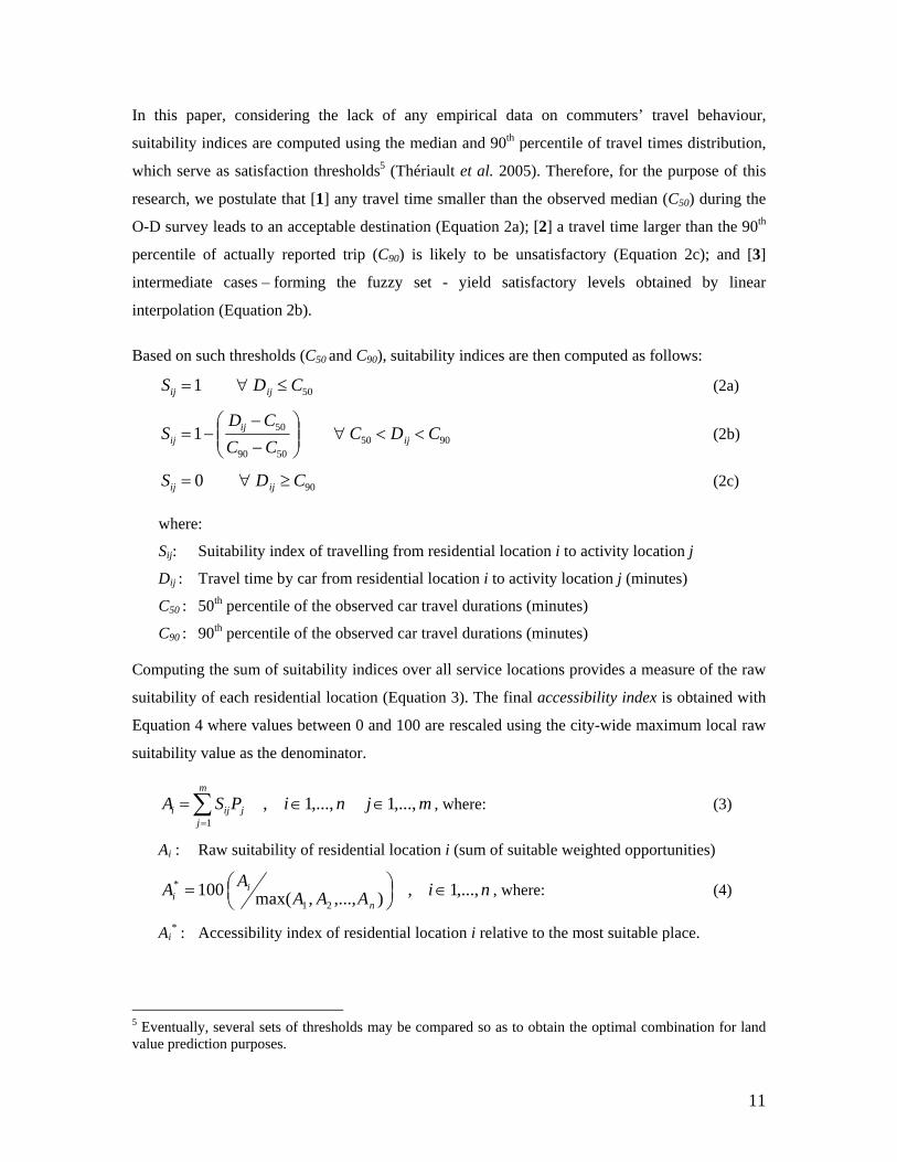
In this paper, considering the lack of any empirical data on commuters’ travel behaviour,
suitability indices are computed using the median and 90th percentile of travel times distribution,
which serve as satisfaction thresholds5 (Thériault et al. 2005). Therefore, for the purpose of this
research, we postulate that [1] any travel time smaller than the observed median (C50) during the
O-D survey leads to an acceptable destination (Equation 2a); [2] a travel time larger than the 90th
percentile of actually reported trip (C90) is likely to be unsatisfactory (Equation 2c); and [3]
intermediate cases – forming the fuzzy set - yield satisfactory levels obtained by linear
interpolation (Equation 2b).
Based on such thresholds (C50 and C90), suitability indices are then computed as follows:
501 CDS ijij ≤∀= (2a)
90505090
501 CDCCCCD
S ijij
ij <<∀⎟⎟⎠
⎞⎜⎜⎝
⎛−−
−= (2b)
900 CDS ijij ≥∀= (2c)
where:
Sij: Suitability index of travelling from residential location i to activity location j
Dij : Travel time by car from residential location i to activity location j (minutes)
C50 : 50th percentile of the observed car travel durations (minutes)
C90 : 90th percentile of the observed car travel durations (minutes)
Computing the sum of suitability indices over all service locations provides a measure of the raw
suitability of each residential location (Equation 3). The final accessibility index is obtained with
Equation 4 where values between 0 and 100 are rescaled using the city-wide maximum local raw
suitability value as the denominator.
mjniPSAm
jjiji ,...,1,...,1,
1
∈∈=∑=
, where: (3)
Ai : Raw suitability of residential location i (sum of suitable weighted opportunities)
niAAAAA
n
ii ,...,1,),...,,max(100
21
* ∈⎟⎠⎞⎜
⎝⎛= , where: (4)
Ai* : Accessibility index of residential location i relative to the most suitable place.
5 Eventually, several sets of thresholds may be compared so as to obtain the optimal combination for land value prediction purposes.
12
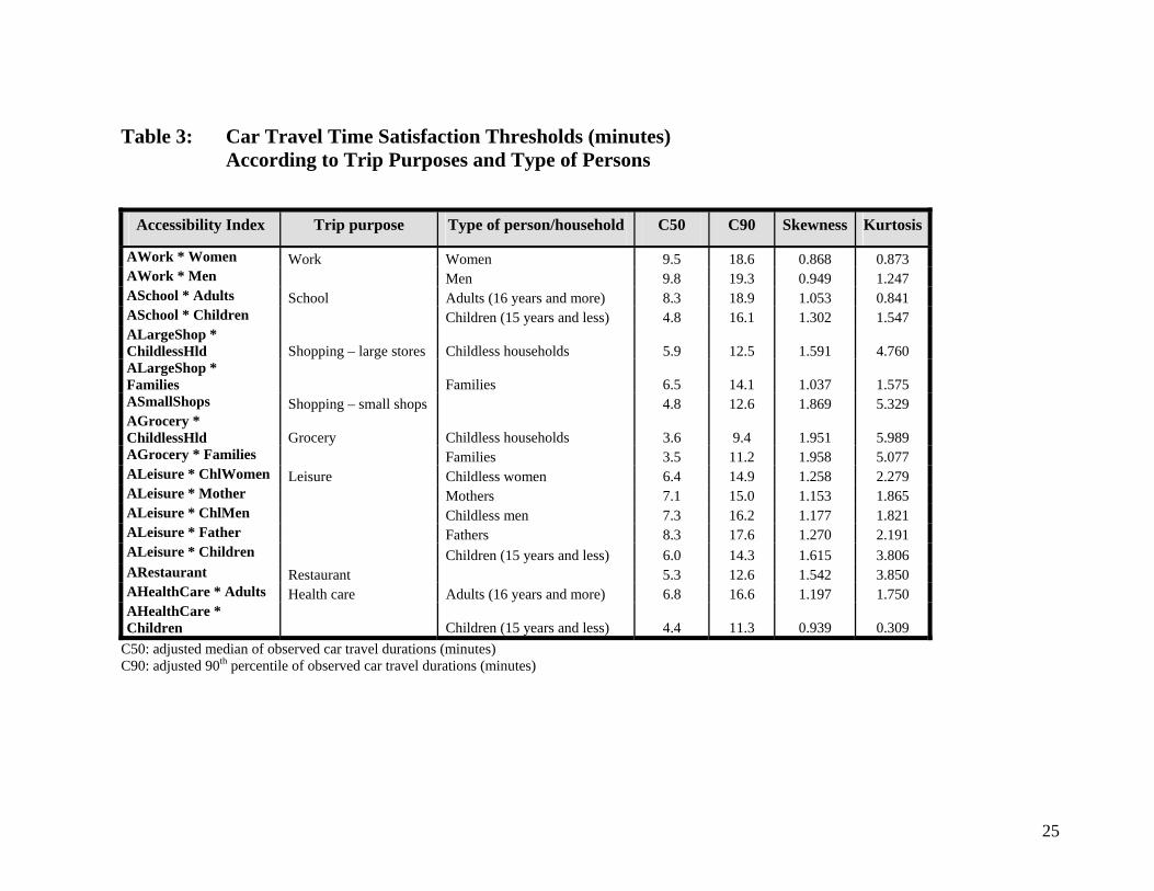
This procedure is applied to every set of trip purpose and type of person/household, as reported in
Table 3. Maps were built for each accessibility index. As an example, Map 1 represents the
overall accessibility to the labour market for women and men.
3.5 Centrality Versus Accessibility: Two Distinct Concepts
All in all, 18 indices were computed to account for centrality (1) and specific subjective
accessibility (17). A correlation analysis performed on all pairs of indices shows that accessibility
and centrality indices are only partly related (correlation coefficients ranging from 0.548 to
0.614), thereby suggesting that these two concepts substantially differ.
Conversely, accessibility indices are highly correlated with each other, with correlation
coefficients ranging from 0.819 to 0.999. Considering the prevalence of the road and street
network in the design of accessibility indices, this is no surprise. More interesting though is the
fact that most pairs of indices show highly significant differences of both ranks and means, as
measured through Wilcoxon and Student t tests, respectively. This reflects the dual nature of
accessibility, which captures at the same time global city-wide patterns and local patterns related
to both the spatial distribution of specific amenities and household perception of their suitability.
This is well exemplified in Table 3 where, for instance, lower and upper suitability thresholds for
leisure activities substantially differ depending on the type of person or household.
3.6 Research Hypotheses
In the above sub-sections, the centrality-accessibility issue has been addressed and the relevance
of complementing supply-driven, or objective, accessibility indices with demand-driven, or
subjective, ones demonstrated. Yet, it remains to be seen whether, and to what extent, such
indices adequately capture the dynamics of travel behaviour: this may best be tested by looking at
the marginal impact they exert on house prices - which are known to internalize any urban
externality - using hedonic modelling. This is the object of Section 4.
More precisely, three research hypotheses are to be tested, based on the above discussion:
Hypothesis H1 : Centrality and accessibility addressing two different realities, both should emerge as statistically significant where used concurrently.
Hypothesis H2 : The willingness to pay for additional accessibility, as measured through house purchase prices, is not homogeneous over space and varies with both trip purpose and type of household.
13
Hypothesis H3 : Because of their specificity with respect to individual and household needs and preferences, demand-driven accessibility indices perform better than supply-driven indices in explaining house price differences.
4. CENTRALITY, ACCESSIBILITY AND HOUSE VALUE MODELLING
4.1 Structuring the Database
Between 1993 and 1996, 16,648 single family houses (bungalows, cottages, attached and row
houses) were sold within the limits of Quebec City and for which transaction prices as well as
house-specific attributes are known. Research hypotheses are to be empirically tested using a
952-unit, spatially stratified and randomly selected, sub-sample on which a phone survey was
conducted in order to get information about the buyer’s profile (household structure, age, income,
choice factors, etc.).
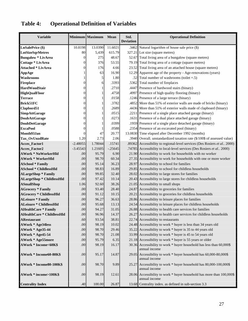
The operational definition of the variables used for hedonic modelling is provided in Table 4.
Sales prices of single-family houses range from $50,000 to $460,000, with an average of roughly
$109,000.
4.2 Modelling House Prices
Due to the high variance on prices (35%), the multiplicative functional form is used for
modelling, with the natural logarithm of sale price as the dependent variable. The first set of
descriptors (LotSizeSqrMetres to ExcaPool) consists of the property specifics previously found to
have a significant impact on house values in this property market (Des Rosiers et al. 2001;
Thériault et al. 2003). A time variable, Month93Jan, is used to account for the temporal drift on
house values during a depressed real estate cycle. Finally, differentials in the local tax burden are
modelled using the overall, unstandardized taxation rate (Tax_OvUnzdRate)6. Over the reference
period, there were 13 different municipalities within the actual Quebec City limits7, each one
having a different yearly tax rate ($/$100 of assessed value).
Accessibility and centrality indices form the second set of descriptors (in grey shading). Physical
accessibility indices (Acces_Factor1 and Acces_Factor2), which were previously shown to exert
highly significant impacts on values (Des Rosiers et al. 2000 and Thériault et al. 2003), are used
6 This rate provides a proxy for the overall tax burden and includes the base property tax rate as well as the pricing of local services. 7 In January 2002, all municipalities were amalgamated into a single one, forming the current Quebec City; since then, two ex-municipalities have decided to de-merge from Quebec City in January 2006.
14
in isolation; the same treatment applies to the centrality index. In order to account for the joint
effects of perceived accessibility indices, trip purposes and household profiles, a series of
interactive variables are designed (Thériault et al. 2005), except for “SmallShop” and
“Restaurant” activities, whose indices are used in isolation.
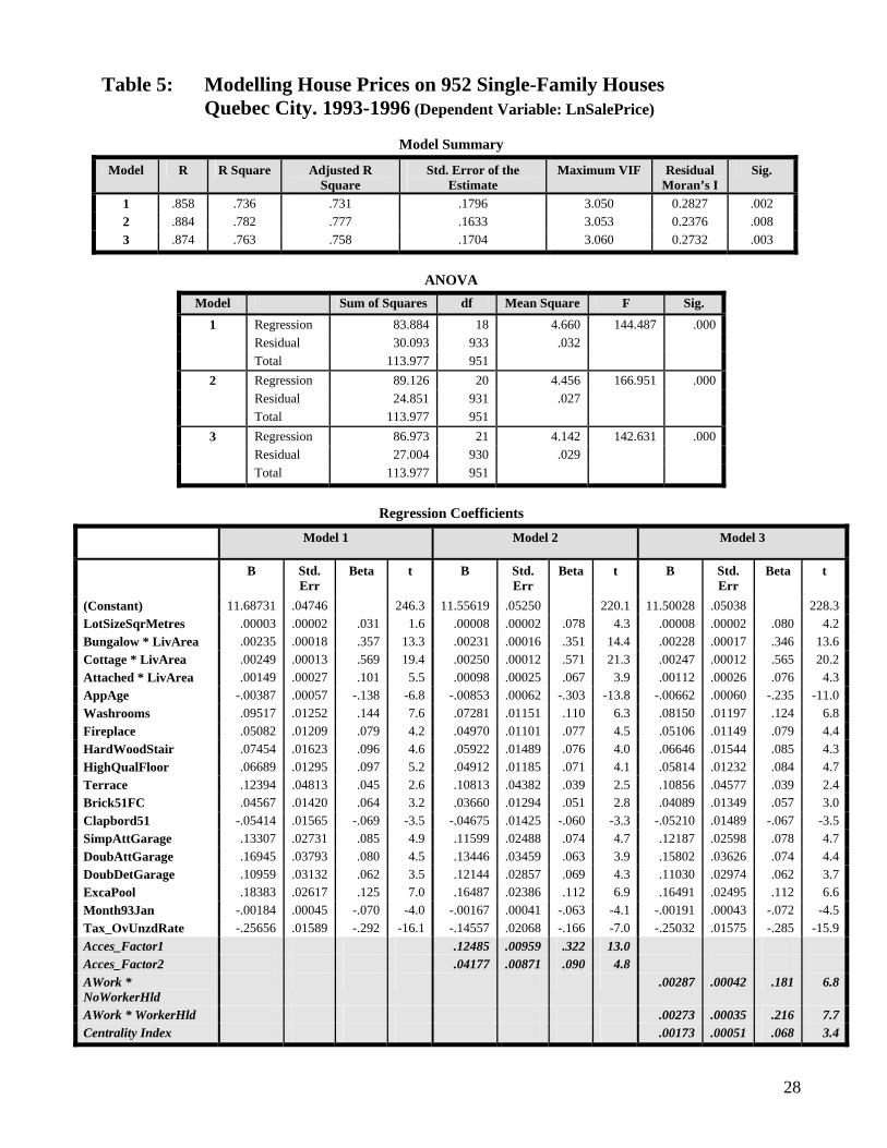
Regression results are reported in Tables 5 and 6. In Table 5, three models are presented: Model 1
includes only building attributes, together with the time and fiscal variables; with Model 2,
objective accessibility is added on; finally, Model 3 substitutes the subjective accessibility indices
pertaining to work places, used in interaction with the household occupational status, for the two
PCA-derived indices used in Model 2; moreover, accessibility indices are complemented by the
centrality index. Regression results obtained for various sets of subjective, mostly interactive,
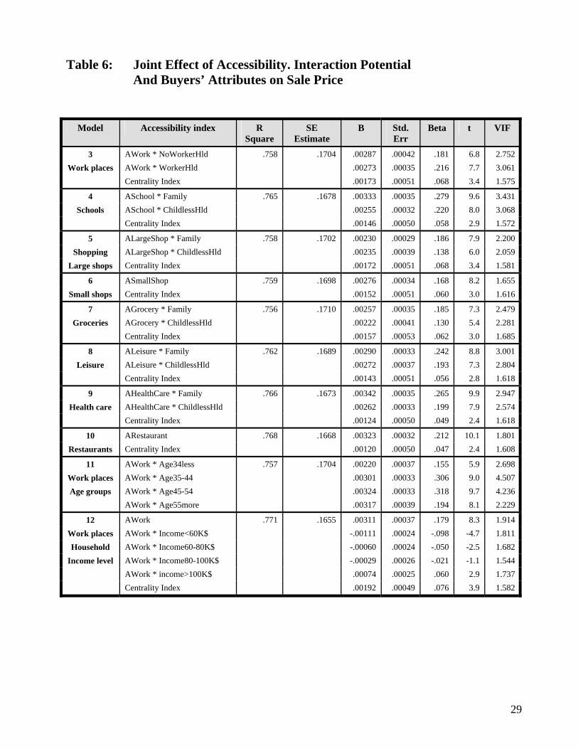
accessibility indices are also reported in Table 6 (Models 3 to 12), together with overall model
performances. Main findings are analyzed in the next sub-section of this paper.
5. ANALYZING AND DISCUSSING MAIN REGRESSION FINDINGS
5.1 Hedonic Price Models
As can be seen from Table 5, the overall explanatory performances range from 0.731 (Model 1)
to 0.777 (Model 2) while models’ relative predictive error (SEE) stands between 16.3% (Model
2) and 18.0% (Model 1). Similar performances are reported for Models 4 to 12. While multi-
collinearity is well under control with a maximum VIF of 3.1 (4.5 for Model 11), the Moran’s I
nevertheless indicates that significant autocorrelation of model residuals still persists after
accessibility is accounted for. This being said, findings suggest that, from a merely statistical
point of view, a supply-driven, physical measure of accessibility, combining travel time
indicators with factor analysis, yields fairly good results.
Turning to individual coefficients, it can be seen from Model 1 that all property-specific
coefficients as well as time and taxation variables emerge as highly significant, with signs and
magnitudes being in line with theoretical expectations. As expected, living area, apparent age and
overall tax rate explain a large proportion of price variations. When added on, Access Factors 1
and 2 (Model 2), reflecting physical accessibility to regional and local amenities, respectively,
substantially improve model performances while leaving most coefficients unchanged. Because
of the excessive multi-collinearity resulting from the inclusion of the centrality index
concurrently to PCA-derived accessibility indices, the former had to be removed from the
equation, which indicates that a very strong structural link exists between supply-driven
15
accessibility and centrality. Both the lot size and apparent age coefficients, however, are raised in
importance and statistical significance while the influence of the fiscal dimension undergoes a
sharp decline, thereby suggesting a strong structural relationship in space among those
dimensions. With respect to the latter, results are consistent with the fact that municipalities
experiencing the lowest overall tax rates are also centrally located and group most of the older
and larger, high-price, houses in the QMA.
Models 3 to 12 - where demand-driven accessibility indices are substituted for physical, travel
time indicators - are the main focus of our analysis. Findings first indicate that both centrality and
accessibility impact significantly, and positively, upon house prices, thereby confirming the
validity of research hypothesis H1 to the effect that “centrality and accessibility addressing two
different realities, both should emerge as statistically significant where used concurrently.” The
relative independence of the two sets of indices is well brought out through the VIF values
reported in Table 6.
Also, findings clearly suggest that, even when controlling for urban centrality, accessibility-to-
services variables emerge as significant, positive determinants of house values while leaving most
other coefficients unchanged – except for the tax rate estimate which has its initial significance
restored. This is so because action-based indices based on fuzzy logic provide a more
comprehensive picture of accessibility, less related to closest amenities than is the case with
components used in Model 2. Table 6 suggests that each specific accessibility index does
contribute in its own way to the shaping of house values and that, as stated in research hypothesis
H2 - which is therefore confirmed -, “the willingness to pay for additional accessibility, as
measured through house purchase prices, is not homogeneous over space and varies with both
trip purpose and type of household.”
Moreover, it is worth noting that demand-driven indices of accessibility far overweight the
centrality index (Beta coefficients of Table 6), which questions the prominence of the CBD as a
location criterion for households. Accessibility to schools and to health care for families, in
particular, as well as accessibility to restaurants are shown to exert a strong influence on prices.
Similarly, people aged 35-54 are willing to pay a substantial market premium to locate at a
reasonable travel time from their work place. Finally, the higher the household income, the
stronger the propensity to lessen work-trip duration (Model 12). This finding, of course, ought to
be interpreted in the light of the household’s income constraint rather than as an indication of a
preference of lower-income households for longer trips. Nevertheless, the latter agree to make a
16
trade-off between, on the one hand, more and cheaper residential land and, on the other hand,
higher commuting costs; hence the negative sign of the pertaining coefficients.
5.2 “Supply-driven” versus “Demand-driven” Accessibility Indices
A major issue of this paper is to investigate whether “action-based”, demand-driven, accessibility
indices could perform better than “supply-driven”, physical, indices at explaining house price
differences. Findings suggest that this is not the case, at least where statistical performances alone
are considered. Therefore, research hypothesis H3 to the effect that “…demand-driven
accessibility indices perform better than supply-driven indices in explaining house price
differences” cannot be confirmed. However, as commented above, the light they shed on house
location choice dynamics is of greater interest than the more “holistic”, but less targeted,
information conveyed by PCA-derived accessibility factors. In addition, in the latter case, the
statistical strength obtained with the regional component (Access Factor 1) may partly stem from
centrality effects which are not explicitly accounted for in Model 2. In other words, if research
hypothesis H3 cannot be confirmed, it cannot be invalidated either.
6. CONCLUSION
6.1 Summary of Findings
This paper is an attempt to bridge the gap between, on the one hand, the mobility behaviour of
households and their perception of accessibility to urban amenities and, on the other hand, house
price dynamics as captured through hedonic modelling. It focuses on analyzing mobility
behaviour of people and estimating their sensitivity to travel time from home to service places so
as to assess their action-based, or demand-driven, accessibility. Accessibility to services for
Quebec City is measured using both supply-driven, physical, indices obtained through factor
analysis and demand-driven indices based on actual trips made by individuals and households.
Applying hedonic modelling to some 952 single-family houses sold between 1993 and 1996,
these two sets of indices are compared and complement a centrality index.
Findings suggest that using factor analysis to derive an “objective” measure of accessibility based
on travel time to the nearest facility yields fairly good results from a merely statistical point of
view. Yet, resorting to action-based accessibility indices in order to assess diversity of choice
within time-distance thresholds (fuzzy logic) allows to investigate commuting patterns and travel
behaviour with greater insight and to design trip-purpose and household profile-specific
indicators of accessibility to urban amenities. Finally, the different nature of centrality and
17
accessibility is well brought out in the fact that both dimensions are shown to affect prices
significantly, although perceptual indices of accessibility far overweight the centrality index,
which questions the prominence of the CBD as a location criterion for households.
For the time being, our conclusions are limited by the fact that only week-day trips (Monday to
Friday) are available for analysis, which has the side effect of considerably underestimating
various kinds of trips, like week-end shopping and leisure ones. We have no firm indication about
the differences in location between week-days as opposed to week-end activities, the latter
benefiting from a larger time frame. Still, this research supports our hypothesis that different
people have a heterogeneous perception of space and thus, will tend to adjust their readiness to
pay for additional centrality/accessibility when choosing their home location, depending on their
needs and preferences.
6.2 Suggestions for Future Research
As this paper suggests, the accessibility concept might be less straightforward than is usually
considered in the literature. Considering it is a paramount determinant of location choices and
property values, it deserves being further investigated in many respects. In particular, the
“subjective” nature of accessibility remains an open issue: while most authors support that it can
be measured on physical, a-contextual grounds, namely through travel distances and times which
are universal references, our research findings point toward the need to bridge a gap between the
spatial dynamics of cities and the utility theory whereby individual preferences form the very
basis of economic decisions.
While budget constraints and cost-minimizing incentives operate as powerful determinants of
individual and household overall behaviour with respect to both commuting and location patterns,
much remains to be known about more subtle, behavioural aspects driving such decisions. The
availability of highly detailed information on households’ daily routine, such as that provided by
O-D surveys and in-depth daily-activity panel surveys, can greatly enhance our understanding of
a phenomenon as complex as accessibility to urban amenities. Finally, relating house prices to
travel behaviour from a space-time perspective, using for instance panel regression techniques, is
also an avenue worth exploring.
18
REFERENCES
Anselin, L., and A. Can, 1986. Model comparison and model validation issues in empirical work on urban density functions. Geographical Analysis, 18: 179-197.
Anselin, L., and S. Rey, 1991. Properties of tests for spatial dependence in linear regression models. Geographical Analysis, 23(2): 112-131.
Anselin, L., and A. Getis, 1992. Spatial statistical analysis and geographic information systems. The Annals of Regional Science, 26: 19-33.
Axhausen, K.W. and T. Gärling, 1992. Activity-based approaches to travel analysis: Conceptual frameworks, models, and research problems. Transport Reviews, 12: 323-341.
Basu, S., and T. G. Thibodeau, 1998. Analysis of spatial autocorrelation in house prices. The Journal of Real Estate Finance and Economics, 17(1): 61-86.
Bateman, I., B. Day, I. Lake and A. Lovett, 2001. The Effect of Road Traffic on Residential Property Values: A Literature Review and Hedonic Pricing Study. Scottish Executive Development Department, Edinburgh, 207 pages.
Boots, B. & P. Kanaroglou, 1988. Incorporating the effects of spatial structure in discrete choice models of migration. Journal of Regional Science, 28: 495-507.
Brueckner, J. and R. Martin, 1997. Spatial mismatch: An equilibrium analysis. Regional Science and Urban Economics, 27: 693-714.
Brunsdon C, Fotheringham AS, Charlton M., 2002. Geographically weighted summary statistics - a framework for localised exploratory data analysis. Computers, Environment and Urban Systems 26: 501-524.
Can, A., 1992. Residential quality assessment: Alternative approaches using GIS. The Annals of Regional Science, 26: 97-110.
Can, A., 1993. Specification and estimation of hedonic housing price models. Regional Science and Urban Economics, 22: 453-474.
Can, A., and I. Megbolugbe, 1997. Spatial dependence and house price index construction. Journal of Real Estate Finance and Economics, 14: 203-222.
Casetti E., 1972. Generating models by the expansion method: Applications to geographical research. Geographical Analysis 4:81-91
Casetti E., 1997. The expansion method, mathematical modeling, and spatial econometrics. International Regional Science Review 20:9-32
Cliff, A. D., R. Martin and J.K. Ord, 1974. Evaluating the friction of distance parameter in gravity models. Regional Studies, 8: 281-286.
Colwell, P.F., S.S. Gujral and C. Coley, 1985. The impact of shopping centers on the value of surrounding properties. Real Estate Issues, 10(1): 35-39.
Colwell, P.F., 1990. Power lines and land values. Journal of Real Estate Research, 5(1): 117-127. Cressie, N. A. C., 1993. Statistics for Spatial Data, New York, Wiley, 900 pages. Curry, L., 1972. Gravity analysis of gravity flows. Regional Studies, 6: 131-147. Des Rosiers, F., 2002. Power Lines, Visual Encumbrance and House Values: A Micro-spatial
Approach to Impact Measurement. The Journal of Real Estate Research, 23:3, 275-300. Des Rosiers, F., and M. Thériault, 1992. Integrating geographic information systems to hedonic
price modelling: An application to the Quebec region. Property Tax Journal, 11(1): 29-57. Des Rosiers, F. and M. Thériault, 1999. House Prices and Spatial Dependence: Towards an
Integrated Procedure to Model Neighbourhood Dynamics. Laval University, Faculty of Business Admin., Québec, Publ. 1999-002, 23 pages.
19
Des Rosiers, F., A. Lagana, M. Thériault and M. Beaudoin, 1996. Shopping centers and house values: An empirical investigation. Journal of Property Valuation and Investment, 14(4): 41-63.
Des Rosiers, F., M. Thériault and P. Villeneuve, 2000. Sorting out access and neighbourhood factors in hedonic price modelling. The Journal of Property Investment and Finance, 18(3): 291-315.
Des Rosiers, F., A. Lagana and M. Thériault, 2001. Size and proximity effects of primary schools on surrounding house values, Journal of Property Research, 18(2): 149-168.
Des Rosiers, François, Marius Thériault, Yan Kestens and Paul-Y. Villeneuve, 2002. Landscaping and House Values: an Empirical Investigation. The Journal of Real Estate Research, Special Issue, 23(1/2): 139-61.
Dubin, R. A., 1988. Estimation of regression coefficients in the presence of spatially autocorrelated error terms. Review of Economics and Statistics, 70: 466-474.
Dubin, R. A., 1992. Spatial autocorrelation and neighbourhood quality. Regional Science and Urban Economics, 22: 433-452.
Dubin, R. A., 1998. Predicting house prices using multiple listings data. The Journal of Real Estate Finance and Economics, 17(1): 35-60.
Dubin, R.A., and C.H. Sung, 1987. Spatial variation in the price of housing: Rent gradients in non-monocentric cities. Urban Studies, 24: 193-204.
Fotheringham A.S., 2000. Context-dependent spatial analysis: A role for GIS? Journal of Geographical Systems 2:71-76
Fotheringham A.S., Charlton ME, Brundson C.F., 1998. Geographical weighted regression: A natural evolution of the expansion method for spatial data analysis. Environment and Planning A 30:1905-1927
Fotheringham A.S., Brundson F.C., Charlton M., 2002. Geographically weighted regression: The analysis of spatially varying relationships. John Wiley and Sons, Chichester
Getis, A., and J. K. Ord, 1992. The analysis of spatial association by use of distance statistics. Geographical Analysis, 24(3): 189-206.
Golledge, R.G., M. P. Kwan and T. Gärling, 1994. Computational process modelling of household travel decision using a geographical information system. Papers in Regional Science, 73(2): 99-117.
Goodchild, M. F., 1998. GIS and disaggregate transportation modelling. Geographical Systems, 5(1): 19-44.
Grieson, R.E. and J.R. White, 1989. The existence and capitalization of neighbourhood externalities: A Reassessment. Journal of Urban Economics, 25(1): 68-76.
Griffith, D. A., 1993. Advanced spatial statistics for analyzing and visualizing geo-references data. International Journal of Geographical Information Systems. 7(2): 107-124.
Guntermann, K.L. and P.F. Colwell, 1983. Property values and accessibility to primary schools. Real Estate Appraiser and Analyst, 49(1): 62-68.
Hägerstrand, T., 1970. What about people in regional science? Papers of the Regional Science Association, 14: 7-16.
Handy, S.L. and D.A. Niemeier, 1997. Measuring accessibility: an exploration of issues and alternatives. Environment and planning A, 29(7): 1175-1194.
Hanson, S., 1995. Getting there: Urban transportation in context. In S. Hanson (Ed.) The Geography of Urban Transportation. New York, The Guilford Press, pp. 3-25.
Hansen, W.G., 1959. How accessibility shapes land use. Journal of American Institute of Planners, 25: 73-76.
20
Helling, A., 1996. The effect of residential accessibility to employment on mens’ and womens’ travel. In Proceedings from the Second National Conference on Womens’ Travel Issues, Baltimore, October 1996, pp. 147-163.
Hickman, E. P., J. P. Gaines and F. J. Ingram, 1984. The influence of neighbourhood quality on residential values. The Real Estate Appraiser and Analyst, 50(2): 36-42.
Hoch, I., and P. Waddell, 1993. Apartment rents: Another challenge to the monocentric model. Geographical Analysis, 25(1): 20-34.
Hotelling, H., 1933. Analysis of a Complex of Statistical Variables into Principal Components. Journal of Educational Psychology, 24: 417-441; 498-520.
Jackson, J.R., 1979. Intraurban variation in the price of housing. Journal of Urban Economics, 6: 464-479.
Johnston, R.J., 1973. On friction of distance and regression coefficients. Area, 5: 187-191. Kestens Y., M. Thériault and F. Des Rosiers, 2004. Impact of surrounding land use and
vegetation on single family house prices. Environment and Planning B: Planning and Design 31(4): 539-567.
Kim, H.M and M.P. Kwan, 2003. Space-time accessibility measures: A geocomputational algorithm with a focus on the feasible opportunity set and possible activity duration. Journal of Geographical Systems, 5: 71-91.
King, Leslie J., 1969. Statistical Analysis in Geography, Prentice-Hall, Englewood Cliffs, N.J. Krantz, D. P., R. D. Waever and T. R. Alter, 1982. Residential tax capitalization: Consistent
estimates using micro-level data. Land Economics, 58(4): 488-496. Landau, U., J. N. Prashker and M. Hirsh, 1981. The effect of temporal constraints in household
travel behaviour. Environment and Planning A, 13: 435-444. Levine, N., 1996. Spatial statistics and GIS. Software tools to quantify spatial patterns. Journal of
the American Planning Association, 62(3): 381-390. Levinson, D.M., 1998. Accessibility and the journey to work. Journal of Transport Geography,
6: 11-21. Levy, J. and M. Lussault, 2003. Dictionnaire de la géographie et de l’espace des sociétés. Paris,
Bélin. Martin, R., 1997. Job decentralization with suburban housing discrimination: An urban
equilibrium model of spatial mismatch. Journal of Housing Economics, 6: 293-317. McMillen, D.P., 2003. The return of centralization to Chicago: Using repeat sales to identify
changes in house price distance gradients. Regional Science and Urban Economics, 33(3): 287-304.
Moran, P. A. P., 1950. Notes on continuous stochastic phenomena. Biometrika, 37: 17-23. Niedercorn, J.H., and N.S. Ammari, 1987. New evidence on the specification and performance of
neoclassical gravity models in the study of urban transportation. The Annals of Regional Sciences, 21(1): 56-64.
Nijkamp, P., L. Van Wissen and A. M. Rima, 1993. A household life cycle model for residential relocation behaviour. Socio-Economic Planning Science, 27(1): 35-53.
Ord, J. K., and A. Getis, 1995. Spatial autocorrelation statistics: Distribution issues and an application. Geographical Analysis, 27(4): 286-306.
Pace, R. K., R. Barry and C. F. Sirmans, 1998. Spatial statistics and real estate. The Journal of Real Estate Finance and Economics, 17(1): 5-14.
21
Páez, A., T. Uchida and K. Miyamoto, 2001. Spatial Association and Heterogeneity Issues in Land Price Models. Urban Studies, 38(9):1493-1508.
Panatier, Y., 1996. Variowin: Software for Spatial Data Analysis in 2D. Statistics and Computing, Springer-Verlag, New York, 91 pages.
Rodriguez, M., C. F. Sirmans and A. P. Marks, 1995. Using geographic information systems to improve real estate analysis. The Journal of Real Estate, 10(2): 163-173.
Rosen, S. (1974) Hedonic Prices and Implicit Markets: Product Differentiation in Pure Competition, Journal of Political Economics, Vol. 82, 34-55.
Rummel, R.J., 1970. Applied Factor Analysis. Evanston, Northwestern University Press.Sirpal, R., 1994. Empirical modelling of the relative impacts of various sizes of shopping centers on the values of surrounding residential properties. Journal of Real Estate Research, 9(4): 487-505.
Shefer, D., 1986. Utility changes in housing and neighbourhood services for households moving into and out of distressed neighbourhoods, Journal of Urban Economics, 19: 107-124.
Sirpal, R., 1994. Empirical modelling of the relative impacts of various sizes of shopping centers on the values of surrounding residential properties. Journal of Real Estate Research, 9(4): 487-505.
Smersh, G.T., and M.T. Smith, 2000. Accessibility changes and urban house price appreciation: A constrained optimization approach to determining distance effects. Journal of Housing Economics, 9(3): 187-196.
So, H.M., R.Y.C. Tse and S. Ganesan, 1997. Estimating the influence of transport on house prices: Evidence from Hong Kong. The Journal of Property Investment and Finance, 15(1): 40-47.
Srour, I.M., K.M. Kockelman and T.P. Dunn, 2002. Accessibility Indices: A Connection to Residential Land Prices and Location Choices. Paper presented at the 81st Annual Meeting of the Transportation Research Board, Jan. 13-17, Washington DC., 19 pages.
Strange, W., 1992. Overlapping neighbourhoods and housing externalities. Journal of Urban Economics, 32: 17-39.
Tabachnick, Barbara G. and L.S. Fidell, 1996. Using Multivariate Statistics. HarperCollins College Publishers, New York, p. 636.
Thériault, M., and F. Des Rosiers, 1995. Combining hedonic modelling, GIS and spatial statistics to analyze residential markets in the Quebec Urban Community. In Proceedings of the Joints European Conference on Geographical Information, EGIS Foundation, March 26-31, The Hague, The Netherlands, 2: 131-136.
Thériault, M., D. Leroux and M. H. Vandersmissen, 1998. Modelling travel route and time within GIS: Its use for planning. In Simulation Technology: Science and Art. Proceedings of the 10th European Simulation Symposium. A. Bargiela and E. Kerckhoffs Eds., The Nottingham-Trent University and Society for Computer Simulation International, October 26-28, 402-407.
Thériault, M., F. Des Rosiers and H. Vandermissen, 1999a. GIS-Based Simulation of Accessibility to Enhance Hedonic Modelling and Property Value Appraisal. Joint IAAO-URISA 1999 Conference, New Orleans, April 11-14, 10 pages.
Thériault, M., M.H. Vandersmissen, M. Lee-Gosselin and D. Leroux, 1999b. Modelling commuter trip length and duration within GIS: Application to an O-D survey. Journal for Geographic Information and Decision Analysis, 3(1): 41-55.
Thériault, M., F. Joerin, P. Villeneuve and F. Bégin, 2001. Modelling accessibility using fuzzy logic within transportation geographical information systems. In Proceedings of the IASTED
22
International Conference on Modelling Identification and Control 2001, 1: 268-275, ACTA Press, Anaheim, California.
Thériault, M., F. Des Rosiers, P.-Y. Villeneuve and Y. Kestens, 2003. Modelling Interactions of Location with Specific Value of Housing Attributes. Property Management, 21(1): 25-62.
Thériault, M. and F. Des Rosiers, 2004. Modelling perceived accessibility to urban amenities using fuzzy logic, transportation GIS and origin-destination surveys. In F. Toppen and P. Prastacos (Eds.) Proceedings of AGILE 2004 7th Conference on Geographic Information Science, Crete University Press, Heraklion, Greece, pp. 475-485.
Thériault M., F. Des Rosiers and F. Joerin. 2005. Modelling Accessibility to Urban Services Using Fuzzy Logic: A Comparative Analysis of Two Methods, Journal of Property Investment and Finance, 23:1, 22-54.
Thrall, G. I., 1993. Using GIS to rate the quality of property tax appraisal. Geo Info Systems, 3(3): 56-62.
Thrall, G. I., and A. P. Marks, 1993. Functional requirements of a geographic information system for performing real estate research and analysis. Journal of Real Estate Literature, 1(1): 49-61.
Thrall, G.I., 2002. Business Geography and New Real Estate Market Analysis. New York: Oxford Press.
Thurstone, L.L., 1947. Multiple Factor Analysis. Chicago, University of Chicago Press. Tiefelsdorf, M., and B. Boots, 1997. A note on the extremities of local Moran's Is and their
impact on global Moran's I. Geographical Analysis, 29(3): 248-257. Tiefelsdorf, M., 2003. Misspecification in interaction model distance decay relations: A spatial
structure effect. Journal of Geographical Systems, 5: 25-50. Timmermans, H., and R. G. Golledge, 1990. Applications of behavioural research on spatial
problems: preferences and choice. Progress in Human Geography, 14: 311-354. Vandersmissen, M.H., P. Villeneuve and M. Thériault, 2003. Analyzing changes in urban form
and commuting times. The Professional Geographer, 55(4): 446-463. Vandersmissen, M.H., M. Thériault and P. Villeneuve, 2004. What about effective access to cars
in motorized households? The Canadian Geographer, 48(4): 488-504. Wiel, M., 1999. La transition urbaine. Le passage de la ville pédestre à la ville motorisée. Liège,
Margada. Yinger, J. H., H. S. Bloom, A. Borsch-Supan and H. F. Ladd, 1987. Property Taxes and House
Values: The Theory and Estimation of Intrajurisdictional Property Tax Capitalization. Studies in Urban Economics, Academic Press, Princeton Univ., 218 pages.
Zhang, Z., and D. Griffith, 1993. Developing user-friendly spatial statistical analysis modules for GIS: An example using ArcView. Computer, Environment and Urban Systems, 21(1): 5-29.
ACKNOWLEDGEMENT
This research was funded by the Canadian SSHRC (Social Sciences and Humanities Research Council) Major Collaborative Research Initiative and Team grants. Authors are grateful to Quebec City Assessment division for giving access to the Assessment role and home transactions data, as well as to Quebec Province’s Ministry of Transport and Réseau de Transport de la Capitale (RTC) for giving access to O-D surveys.
23
Table 1: Factor Analysis On Access Attributes
Total Variance ExplainedExtraction Sums of Squared Loadings Rotation Sums of Squared Loadings
Component Total % of Variance Cumulative % Total % of Variance Cumulative %1 9.683 64.556 64.556 6.313 42.086 42.0862 1.668 11.122 75.678 5.039 33.592 75.678
Extraction Method: Principal Component Analysis.
Rotated Component Matrix a
.6466 .3518
.7584 .5554
.5572 .7276
.5455 .6708
.3511 .7967
.9107 .2421
.9156 .2737
.6101 .5335
.8933 .1427
.3198 .7009
.4070 .7762
.0106 .7237
.2733 .8475
.8009 .2968
.8753 .3606
Travel time to nearest highway entrance by car (minutes)Travel time to nearest regional shopping center by car (minutes)Travel time to nearest local shopping center by car (minutes)Travel time to nearest neighbourhood shopping center by car (minutes)Travel time to nearest highschool by car (minutes)Travel time to nearest college or university by car (minutes)Travel time to Laval University by car (minutes)Travel time to Downtown Quebec by car (minutes)Travel time to Downtown Ste-Foy by car (minutes)Travel time to La Capitale shopping center by car (minutes)Walking time to nearest neighbourhood shopping center (minutes)Walking time to nearest primary school (minutes)Walking time to nearest highschool (minutes)Walking time to nearest college or university (minutes)Walking time to Laval University (minutes)
1 2Component
Extraction Method: Principal Component Analysis. Rotation Method: Varimax with Kaiser Normalization.
Rotation converged in 3 iterations.a.
24
Table 2a: Travel Times By Trip Purpose (minutes)
Trip purpose Nb. of trips Average time Variance Work 12,947 10.53 40.65 School 2,386 7.55 41.00 Shopping – large stores 3,249 6.98 22.52 Shopping – small shops 2,271 6.24 26.78 Grocery 2,967 4.69 15.69 Leisure 3,204 8.02 30.64 Restaurant 1,635 6.51 23.03 Health care 943 8.04 33.90
By Type of Person/Household (Two-tailed Student test for differences between means using unrelated samples)
Trip purpose Group Average
duration(min.)
versus Group Average duration
(min.)
Student Sig.
Work 6,371 Women 10.30 6,576 Men 10.76 4.048 0.000School 407 Adults 9.89 1,979 Children 7.07 8.196 0.000Shopping – large stores 2,521 Childless households 6.81 601 Families 7.54 3.414 0.001Shopping – small shops No significant differences among groups Grocery 2,229 Childless households 4.52 669 Families 5.15 3.612 0.000Leisure 1,057 Childless women 7.59 325 Mothers 8.28 2.072 0.038 1,013 Childless men 8.25 268 Fathers 9.34 2.706 0.007 1,539 Women 7.72 1,665 Men 8.33 3.132 0.002 2,663 Adults 8.10 541 Children 7.59 1.971 0.049Health care 859 Adults 8.26 84 Children 5.76 3.781 0.000Restaurant No significant differences among groups
25
Table 3: Car Travel Time Satisfaction Thresholds (minutes) According to Trip Purposes and Type of Persons
Accessibility Index Trip purpose Type of person/household C50 C90 Skewness Kurtosis
AWork * Women Work Women 9.5 18.6 0.868 0.873 AWork * Men Men 9.8 19.3 0.949 1.247 ASchool * Adults School Adults (16 years and more) 8.3 18.9 1.053 0.841 ASchool * Children Children (15 years and less) 4.8 16.1 1.302 1.547 ALargeShop * ChildlessHld Shopping – large stores Childless households 5.9 12.5 1.591 4.760 ALargeShop * Families Families 6.5 14.1 1.037 1.575 ASmallShops Shopping – small shops 4.8 12.6 1.869 5.329 AGrocery * ChildlessHld Grocery Childless households 3.6 9.4 1.951 5.989 AGrocery * Families Families 3.5 11.2 1.958 5.077 ALeisure * ChlWomen Leisure Childless women 6.4 14.9 1.258 2.279 ALeisure * Mother Mothers 7.1 15.0 1.153 1.865 ALeisure * ChlMen Childless men 7.3 16.2 1.177 1.821 ALeisure * Father Fathers 8.3 17.6 1.270 2.191 ALeisure * Children Children (15 years and less) 6.0 14.3 1.615 3.806 ARestaurant Restaurant 5.3 12.6 1.542 3.850 AHealthCare * Adults Health care Adults (16 years and more) 6.8 16.6 1.197 1.750 AHealthCare * Children Children (15 years and less) 4.4 11.3 0.939 0.309
C50: adjusted median of observed car travel durations (minutes) C90: adjusted 90th percentile of observed car travel durations (minutes)
26
Map 1a: Relative Accessibility by Car to Work Places for Adult Women
0 5 10
kilometres
Work Places
13 000
6 5001 300
Accessibility Index (%)90 to 10080 to 9070 to 8060 to 7050 to 6040 to 5030 to 4020 to 3010 to 20
0 to 10
Map 1b: Relative Accessibility by Car to Work Places for Adult Men
0 5 10
kilometres
Work Places
13 000
6 5001 300
Accessibility Index (%)90 to 10080 to 9070 to 8060 to 7050 to 6040 to 5030 to 4020 to 3010 to 20
0 to 10
1090,080,0
70,060,0
50,040,0
30,020,0
10,00,0
Num
ber o
f sol
d bu
ildin
gs (1
987-
96)
2500
2000
1500
1000
500
0
SMN
1090,080,0
70,060,0
50,040,0
30,020,0
10,00,0
Num
ber o
f bui
ldin
gs
2500
2000
1500
1000
500
0
1090,080,0
70,060,0
50,040,0
30,020,0
10,00,0
Num
ber o
f sol
d bu
ildin
gs (1
987-
96)
2500
2000
1500
1000
500
0
27
Table 4: Operational Definition of Variables
Variable Minimum Maximum Mean Std. Deviation
Operational Definition
LnSalePrice ($) 10.8198 13.0390 11.6021 .3462 Natural logarithm of house sale price ($) LotSizeSqrMetres 80 5,439 615.79 327.21 Lot size (square metres) Bungalow * LivArea 0 275 48.67 52.67 Total living area of a bungalow (square metres) Cottage * LivArea 0 376 53.55 79.19 Total living area of a cottage (square metres) Attached * LivArea 0 176 4.66 23.52 Total living area of an attached house (square metres) AppAge 1 63 16.90 12.29 Apparent age of the property - Age-renovations (years) Washrooms 1 5 1.80 .52 Total number of washrooms (toilet =.5) Fireplace 0 6 .3393 .5362 Total number of fireplaces HardWoodStair 0 1 .2710 .4447 Presence of hardwood stairs (binary) HighQualFloor 0 1 .4758 .4997 Presence of high quality flooring (binary) Terrace 0 1 .0158 .1246 Presence of a large terrace (binary) Brick51FC 0 1 .3782 .4852 More than 51% of exterior walls are made of bricks (binary) Clapbord51 0 1 .2689 .4436 More than 51% of exterior walls made of clapboard (binary) SimpAttGarage 0 1 .0515 .2211 Presence of a single place attached garage (binary) DoubAttGarage 0 1 .0273 .1631 Presence of a dual place attached garage (binary) DoubDetGarage 0 1 .0399 .1959 Presence of a single place detached garage (binary) ExcaPool 0 1 .0588 .2354 Presence of an excavated pool (binary) Month93Jan 0 47 20.77 13.0830 Time elapsed after December 1992 (months) Tax_OvUnzdRate 1.20 2.73 2.06 .3940 Overall. unstandardized taxation rate ($/100$ of assessed value) Acces_Factor1 -2.48055 1.78044 .15741 .89362 Accessibility to regional-level services (Des Rosiers et al.. 2000)Acces_Factor2 -3.45543 1.21605 -.25645 .74785 Accessibility to local-level services (Des Rosiers et al.. 2000) AWork * NoWorkerHld .00 95.79 6.90 21.90 Accessibility to work for households with no worker AWork * WorkerHld .00 98.70 60.34 27.35 Accessibility to work for households with one or more worker ASchool * Family .00 95.14 36.23 28.97 Accessibility to school for families ASchool * ChildlessHld .00 98.83 16.89 29.85 Accessibility to school for childless households ALargeShop * Family .00 99.85 32.40 28.02 Accessibility to large stores for families ALargeShop * ChildlessHld .00 97.42 10.14 20.43 Accessibility to large stores for childless households ASmallShop 1.06 92.60 38.26 21.05 Accessibility to small shops AGrocery * Family .00 93.40 28.40 24.87 Accessibility to groceries for families AGrocery * ChildlessHld .00 91.12 10.15 20.21 Accessibility to groceries for childless households ALeisure * Family .00 96.27 36.63 28.86 Accessibility to leisure places for families ALeisure * ChildlessHld .00 95.68 13.13 24.54 Accessibility to leisure places for childless households AHealthCare * Family .00 94.27 31.05 26.88 Accessibility to health care services for families AHealthCare * ChildlessHld .00 96.96 14.37 26.27 Accessibility to health care services for childless households ARestaurant .60 93.54 38.81 22.74 Accessibility to restaurants AWork * Age34less .00 98.19 10.02 24.48 Accessibility to work * buyer is less than 34 years old AWork * Age35-44 .00 98.70 29.46 35.22 Accessibility to work * buyer is 35 to 44 years old AWork * Age45-54 .00 98.70 21.08 33.99 Accessibility to work * buyer is 45 to 54 years old AWork * Age55more .00 95.79 6.35 21.18 Accessibility to work * buyer is 55 years or older AWork * Income<60K$ .00 98.19 16.17 30.36 Accessibility to work * buyer household has less than 60,000$
annual income AWork * Income60-80K$ .00 95.17 14.87 29.05 Accessibility to work * buyer household has 60,000-80,000$
annual income AWork * Income80-100K$ .00 98.70 9.89 25.27 Accessibility to work * buyer household has 80,000-100,000$
annual income AWork * income>100K$ .00 98.19 12.61 28.06 Accessibility to work * buyer household has more than 100,000$
annual income Centrality Index .40 100.00 26.87 13.68 Centrality index. as defined in sub-section 3.3
28
Table 5: Modelling House Prices on 952 Single-Family Houses Quebec City. 1993-1996 (Dependent Variable: LnSalePrice)


![DOCUMENT DE TRAVAIL 2014-005 - Université Laval · The Vehicle Routing Problem with Pauses ... similar to a multi-period problem [1]. ... Vertex 0 corresponds to the depot, while](https://static.documents.pub/doc/80x56/5b85bb0c7f8b9a9a4d8b5206/document-de-travail-2014-005-universite-the-vehicle-routing-problem-with.jpg)

