Hindawi Publishing Corporation Mathematical Problems in Engineering Volume 2010, Article ID 842896, 20 pages doi:10.1155/2010/842896 Research Article Dynamic Tracking with Zero Variation and Disturbance Rejection Applied to Discrete-Time Systems Renato de Aguiar Teixeira Mendes, 1 Edvaldo Assunc ¸˜ ao, 1 Marcelo C. M. Teixeira, 1 and Cristiano Q. Andrea 2 1 Department of Electrical Engineering, Universidade Estadual Paulista (UNESP), Campus of Ilha Solteira, 15385-000 Ilha Solteira, Brazil 2 Academic Department of Electronics, Federal Technological University of Paran´ a (UTFPR), 80230910 Curitiba, PR, Brazil Correspondence should be addressed to Renato de Aguiar Teixeira Mendes, [email protected]Received 1 December 2009; Revised 29 June 2010; Accepted 9 December 2010 Academic Editor: Fernando Lobo Pereira Copyright q 2010 Renato de Aguiar Teixeira Mendes et al. This is an open access article distributed under the Creative Commons Attribution License, which permits unrestricted use, distribution, and reproduction in any medium, provided the original work is properly cited. The problem of signal tracking in discrete linear time invariant systems, in the presence of a disturbance signal in the plant, is solved using a new zero-variation methodology. A discrete-time dynamic output feedback controller is designed in order to minimize the H ∞ norm between the exogen input and the output signal of the system, such that the effect of the disturbance is attenuated. Then, the zeros modification is used to minimize the H ∞ norm from the reference input signal to the error signal. The error is taken as the difference between the reference and the output signal. The proposed design is formulated in linear matrix inequalities LMIsframework, such that the optimal solution of the stated problem is obtained. The method can be applied to plants with delay. The control of a delayed system illustrates the effectiveness of the proposed method. 1. Introduction In a control systems theory, the design of controller using pole placement of closed loop discrete-time systems can be easily done. In 1a controller using pole placement is used to obtain an exact plot of complementary root locus, of biproper open-loop transfer functions, using only well-known root locus rules. However, the problem of zero placement is not very much studied by the control researchers. In 2a discrete-time pole placement is obtained by a control design technique that uses simple and multirate sample. The methodology proposed
Transcript
Hindawi Publishing CorporationMathematical Problems in EngineeringVolume 2010, Article ID 842896, 20 pagesdoi:10.1155/2010/842896
Research ArticleDynamic Tracking withZero Variation and Disturbance RejectionApplied to Discrete-Time Systems
Renato de Aguiar Teixeira Mendes,1 Edvaldo Assuncao,1Marcelo C. M. Teixeira,1 and Cristiano Q. Andrea2
1 Department of Electrical Engineering, Universidade Estadual Paulista (UNESP), Campus of Ilha Solteira,15385-000 Ilha Solteira, Brazil
2 Academic Department of Electronics, Federal Technological University of Parana (UTFPR),80230910 Curitiba, PR, Brazil
Correspondence should be addressed to Renato de Aguiar Teixeira Mendes,[email protected]
Received 1 December 2009; Revised 29 June 2010; Accepted 9 December 2010
Academic Editor: Fernando Lobo Pereira
Copyright q 2010 Renato de Aguiar Teixeira Mendes et al. This is an open access articledistributed under the Creative Commons Attribution License, which permits unrestricteduse, distribution, and reproduction in any medium, provided the original work is properly cited.
The problem of signal tracking in discrete linear time invariant systems, in the presence of adisturbance signal in the plant, is solved using a new zero-variation methodology. A discrete-timedynamic output feedback controller is designed in order to minimize the H∞ norm betweenthe exogen input and the output signal of the system, such that the effect of the disturbance isattenuated. Then, the zeros modification is used to minimize the H∞ norm from the referenceinput signal to the error signal. The error is taken as the difference between the reference and theoutput signal. The proposed design is formulated in linear matrix inequalities (LMIs) framework,such that the optimal solution of the stated problem is obtained. The method can be applied toplants with delay. The control of a delayed system illustrates the effectiveness of the proposedmethod.
1. Introduction
In a control systems theory, the design of controller using pole placement of closed loopdiscrete-time systems can be easily done. In [1] a controller using pole placement is used toobtain an exact plot of complementary root locus, of biproper open-loop transfer functions,using only well-known root locus rules. However, the problem of zero placement is not verymuch studied by the control researchers. In [2] a discrete-time pole placement is obtained by acontrol design technique that uses simple and multirate sample. The methodology proposed
2 Mathematical Problems in Engineering
in [3] preserves the H2 state feedback controller optimality by pole placement in a Z plainregion specified in design. In the field of discrete-time systems pole placement we find [4],where discrete adaptative controllers are designed considering arbitrary zero location. Also,in [5] a class of nonmodeled dynamics is controlled using a zero placement.
In [6] a methodology is proposed using zero and pole placement for discrete-timesystems, to obtain the signal tracking and disturbance rejection, respectively. However, forthe signal tracking problem, when a state feedback estimator is proposed, a modificationoccurs in H∞-norm value obtained with the initial controller that provides the disturbancerejection. Themethodology proposed in this paper has the advantage of maintaining theH∞-norm value obtained with the initial controller for the signal tracking problem.
The problem of signal tracking, in the presence of disturbance signal for continuous-time plant, was solved in [7], using a zero variation methodology. A methodology witha simpler mathematic formulation is proposed in [8]. The signal tracking problem withdisturbance rejection in discrete-time systems is solved by an analytic method in [9], however,the mathematic formulation is complex and a frequency selective tracking is not presented asproposed in this manuscript. In [10] the use of linear matrix inequalities (LMIs) is consideredin design of controllers, filters and stability study. Also, in [11], LMIs are used for the designof a dynamic output feedback controller in order to guarantee the asymptotic stability of acontinuous-time system and minimize the upper bound of a given quadratic cost function.Furthermore, the LMI formulation has been used in several engineering problems (see, e.g.,[12–20]).
This manuscript proposes a formulation of a signal tracking with disturbance rejectionoptimization problem for discrete-time systems in the linear matrix inequalities framework,such that the optimal solution of the stated control problem is obtained. The proposedmethodis simpler than the other tracking techniques, and the main result is that when the problemis feasible the optimal solution is obtained with small computation effort, as the LMIs canbe solved using linear programming algorithms, with polynomial convergence. The softwareMATLAB [21] is used to find the LMI solutions, when the problem is feasible. The control ofa delayed system illustrates the effectiveness of the proposed method.
2. Statement of the Problems
Consider a controllable and observable linear time-invariant multi-input multi-output(MIMO) discrete-time system,
x(k + 1) = Ax(k) + Buu(k) + Bww(k),
y(k) = C1x(k),
z(k) = C2x(k), x(0) = 0, k ∈ [0;∞),
(2.1)
where A ∈ �n×n, Bu ∈ �n×p, Bw ∈ �n×q, C1 ∈ �m×n, C2 ∈ �m×n, x(k) is the state vector, y(k)is the output vector, u(k) is the control input and w(k) is the disturbance input (exogenousinput).
Problem 1. The disturbance rejection problem for discrete-time systems, using the dynamicoutput feedback of the system described in (2.1), is the following: minimize the upper bound
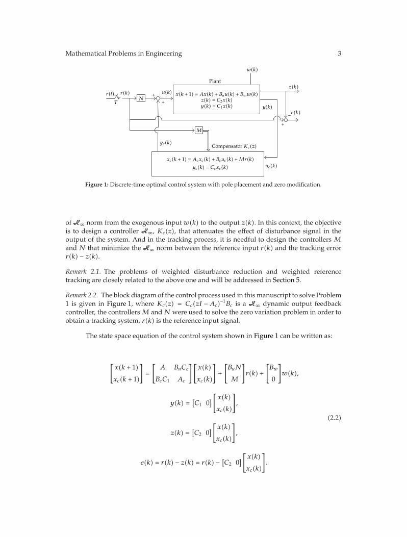
Figure 1: Discrete-time optimal control system with pole placement and zero modification.
of H∞ norm from the exogenous input w(k) to the output z(k). In this context, the objectiveis to design a controller H∞, Kc(z), that attenuates the effect of disturbance signal in theoutput of the system. And in the tracking process, it is needful to design the controllers Mand N that minimize the H∞ norm between the reference input r(k) and the tracking errorr(k) − z(k).
Remark 2.1. The problems of weighted disturbance reduction and weighted referencetracking are closely related to the above one and will be addressed in Section 5.
Remark 2.2. The block diagramof the control process used in this manuscript to solve Problem1 is given in Figure 1, where Kc(z) = Cc(zI −Ac)−1Bc is a H∞ dynamic output feedbackcontroller, the controllersM andN were used to solve the zero variation problem in order toobtain a tracking system, r(k) is the reference input signal.
The state space equation of the control system shown in Figure 1 can be written as:
[x(k + 1)
xc(k + 1)
]=
[A BuCc
BcC1 Ac
][x(k)
xc(k)
]+
[BuN
M
]r(k) +
[Bw
0
]w(k),
y(k) =[C1 0
][ x(k)xc(k)
],
z(k) =[C2 0
][ x(k)xc(k)
],
e(k) = r(k) − z(k) = r(k) − [C2 0
][ x(k)xc(k)
].
(2.2)
4 Mathematical Problems in Engineering
Rewriting the system (2.2) in a compact form, it follows that:
x(k + 1) = Amxm(k) + Bmr(k) + Bnw(k),
e(k) = −Cmx(k) +Dmr(k),
z(k) = Cmx(k),
(2.3)
where
xm(k) =
[x(k)
xc(k)
], Am =
[A BuCc
BcC1 Ac
], Dm = 1, (2.4)
Bm =
[BuN
M
], Bn =
[Bw
0
], Cm =
[C2 0
]. (2.5)
Using the Z-transform in order to solve the system (2.3), consider the initial conditionsequal to zero. One obtains the transfer function between input signals (reference inputand exogenous input) and the measured output of the system as showed in the followingequation:
For the transfer function fromw(Z) to z(Z) in (2.6), theminimization ofH∞ norm is obtainedwith the initial design of H∞ controller, that implies in the minimization of the perturbationeffect in to the system output.
Figure 1 shows the addition of the termMr(k) in the structure of theKc(z) controller.The purpose of the controllerM is only to change the zeros of the transfer function from r(k)to u(k) and it does not change the poles obtained in the initial design of Kc(z). The transferfunction from W(z) to Z(z) is not changed by N or M, according to (2.4) and (2.5). In thisway the performance of theH∞ norm controller is not affected.
For the optimal tracking design, the relation between error signal and reference signaldescribed in (2.7) is considered, making the perturbation signalW(z) equal to zero in (2.6),
Hm(z) =E(z)R(z)
= −Cm(zI −Am)−1Bm +Dm. (2.7)
In this case, using the zero modification one can design a tracking system that minimizes theH∞ norm between the reference input r(k) and the tracking error r(k) − z(k). In Section 4,motivated by the work in [22], we show that M and N modify the zeros from r(k) to u(k).The process of the zerosmodification does not interfere in the disturbance rejection. Thereforein agreement with (2.6), Bm has no influence on the transfer function from W(z) to Z(z). In(2.6) one uses the zeros location, by the specifications of theN andM in Bm, in the process ofminimization of the H∞ norm of the transfer function between the reference signal and thetracking error.
Mathematical Problems in Engineering 5
3. H∞ Dynamic Output Feedback Controller Design
The following theorem leads to a new method to design the Kc(z) in a LMI framework,and the goal is to attenuate the effects of exogenous signal in the output of discrete-timesystems. By using [23], a pole placement constraint region with radius r and center in (−q, 0)is required and used in this work to provide the designer with an expedite way to keep thecontroller gains within appropriate bounds.
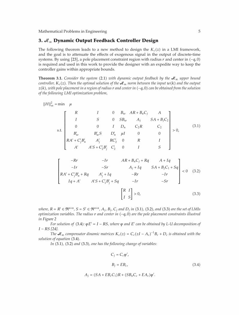
Theorem 3.1. Consider the system (2.1) with dynamic output feedback by the H∞ upper boundcontroller, Kc(z). Then the optimal solution of theH∞ norm between the input w(k) and the outputz(k), with pole placement in a region of radius r and center in (−q, 0) can be obtained from the solutionof the following LMI optimization problem,
‖H‖2∞ =min μ
s.t.
⎡⎢⎢⎢⎢⎢⎢⎢⎢⎢⎢⎢⎣
R I 0 Bw AR + BuCj A
I S 0 SBw Aj SA + BjC2
0 0 I Dn C2R C2
B′w B′
wS D′n μI 0 0
RA′ + C′jB
′u A′
j RC′2 0 R I
A′ A′S +C′2B
′j C′
2 0 I S
⎤⎥⎥⎥⎥⎥⎥⎥⎥⎥⎥⎥⎦> 0,
(3.1)
⎡⎢⎢⎢⎢⎢⎣
−Rr −Ir AR + BuCj + Rq A + Iq
−Ir −Sr Aj + Iq SA + BjC1 + Sq
RA′ + C′jB
′u + Rq A′
j + Iq −Rr −IrIq +A′ A′S + C′
1B′j + Sq −Ir −Sr
⎤⎥⎥⎥⎥⎥⎦ < 0 (3.2)
[R I
I S
]> 0, (3.3)
where, R = R′ ∈ �n×n, S = S′ ∈ �n×n,Aj , Bj , Cj andDj in (3.1), (3.2), and (3.3) are the set of LMIsoptimization variables. The radius r and center in (−q, 0) are the pole placement constraints illustredin Figure 2
For solution of (3.4): ψE′ = I − RS, where ψ and E′ can be obtained by L-U decomposition ofI − RS [24].
The H∞ compensator dinamic matrices Kc(z) = Cc(zI − Ac)−1Bc + Dc is obtained with thesolution of equation (3.4).
In (3.1), (3.2) and (3.3), one has the following change of variables:
Cj = Ccψ′,
Bj = EBc,
Aj = (SA + EBcC1)R + (SBuCc + EAc)ψ ′.
(3.4)
6 Mathematical Problems in Engineering
−1 −0.8 −0.6 −0.4 −0.2 0 0.2 0.4 0.6 0.8 1
−1−0.8−0.6−0.4−0.2
0
0.2
0.4
0.6
0.8
1
−q
r
Re(z)
Im(z)
Figure 2: The pole placement region in the Z plane.
Proof. A realization of dynamic output feedback system Rwz is as followings:
Rwz = Ccl + (zI −Acl)−1Bcl, (3.5)
where
Acl =
[A BuCc
BcC1 Ac
], Bcl =
[Bw
0
], Ccl =
[C2 0
]. (3.6)
The optimization problem below described in LMI framework [25], is used to design theH∞compensator with pole placement constraints
‖H‖2∞ =min μ
s.t.
⎡⎢⎢⎢⎢⎢⎣
Q 0 Bcl AclQ
0 I D CclQ
B′cl D′ μI 0
QA′cl QC
′cl 0 Q
⎤⎥⎥⎥⎥⎥⎦ > 0,
(3.7)
[ −rpQ AclQ + qQ
Qq + QA′cl −rpQ
]< 0,
Q = Q′ > 0,
μ > 0.
(3.8)
However, a high computational effort is needed to solve this problem, because theoptimization problems (3.7) and (3.8) are described as a solution of BMIs. Then, using a linear
Mathematical Problems in Engineering 7
transformation, the problem can be easily solved, based on LMI framework. First, the matrixQ and its inverse are considered as follows
Q =
[R ψ
ψ ′ J
], Q−1 =
[S E
E′ S
], (3.9)
where R = R′ ∈ �n×n, S = S′ ∈ �n×n, and
QΓ2 = Γ1, with Γ1 =
[R I
ψ ′ 0
], Γ2 =
[I S
0 E′
]. (3.10)
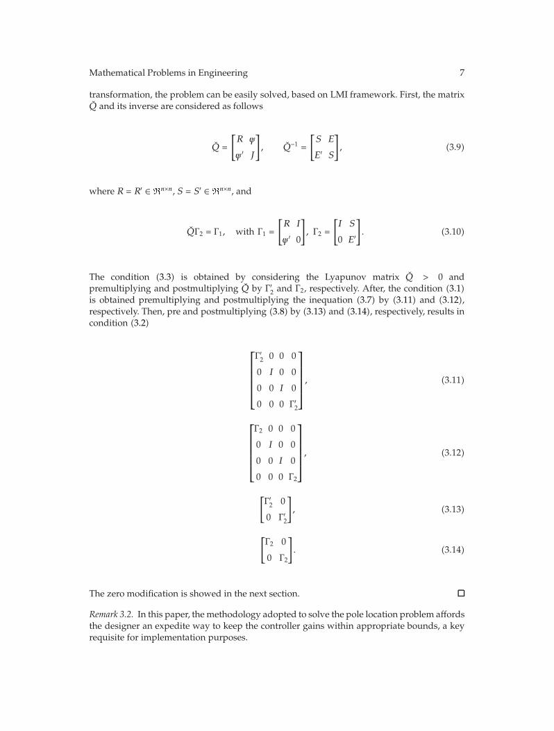
The condition (3.3) is obtained by considering the Lyapunov matrix Q > 0 andpremultiplying and postmultiplying Q by Γ′2 and Γ2, respectively. After, the condition (3.1)is obtained premultiplying and postmultiplying the inequation (3.7) by (3.11) and (3.12),respectively. Then, pre and postmultiplying (3.8) by (3.13) and (3.14), respectively, results incondition (3.2)
⎡⎢⎢⎢⎢⎢⎣
Γ′2 0 0 0
0 I 0 0
0 0 I 0
0 0 0 Γ′2
⎤⎥⎥⎥⎥⎥⎦, (3.11)
⎡⎢⎢⎢⎢⎢⎣
Γ2 0 0 0
0 I 0 0
0 0 I 0
0 0 0 Γ2
⎤⎥⎥⎥⎥⎥⎦, (3.12)
[Γ′2 0
0 Γ′2
], (3.13)
[Γ2 0
0 Γ2
]. (3.14)
The zero modification is showed in the next section.
Remark 3.2. In this paper, the methodology adopted to solve the pole location problem affordsthe designer an expedite way to keep the controller gains within appropriate bounds, a keyrequisite for implementation purposes.
8 Mathematical Problems in Engineering
r(k)N
u(k) x(k + 1) = Ax(k) + Buu(k)y(k) = C1x(k)
y(k)
yc(k)
xc(k + 1) = Acxc(k) + Bcuc(k) +Mr(k)uc(k)
+
+
M
T
r(t)
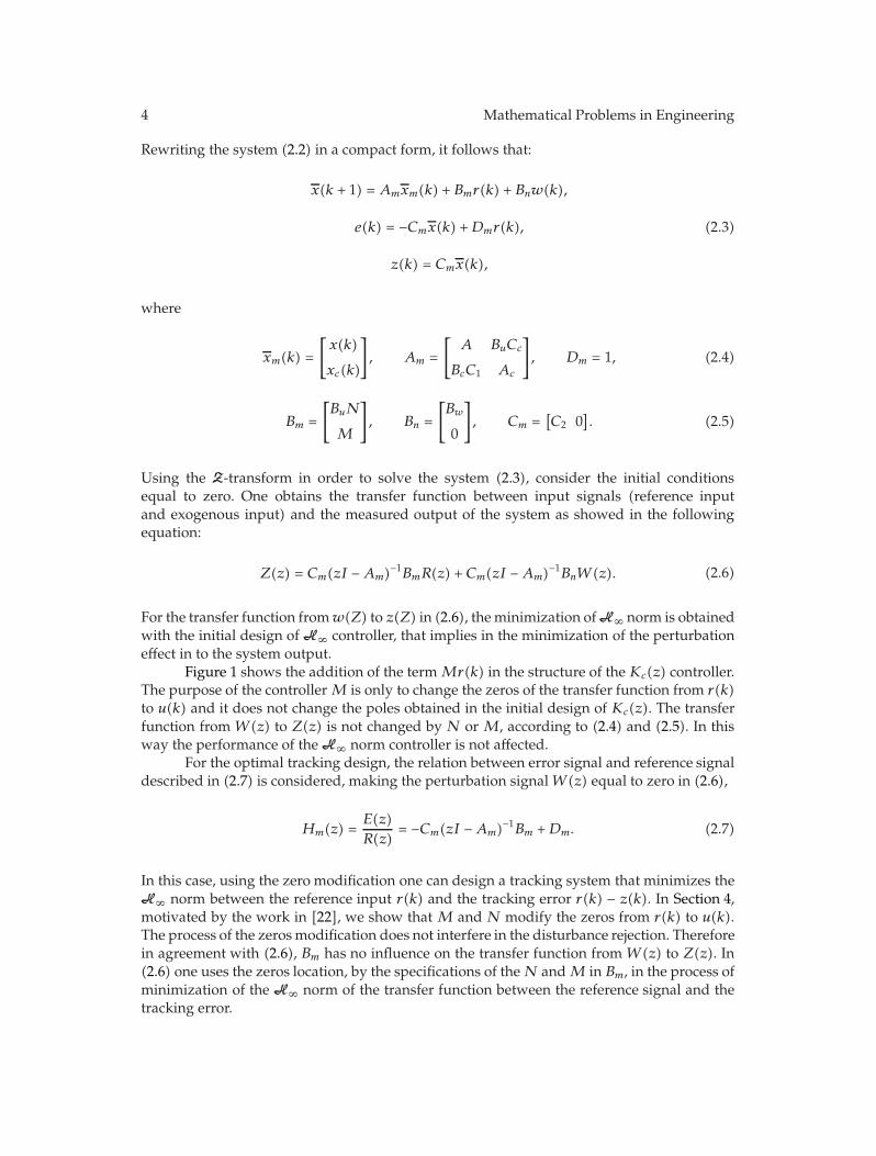
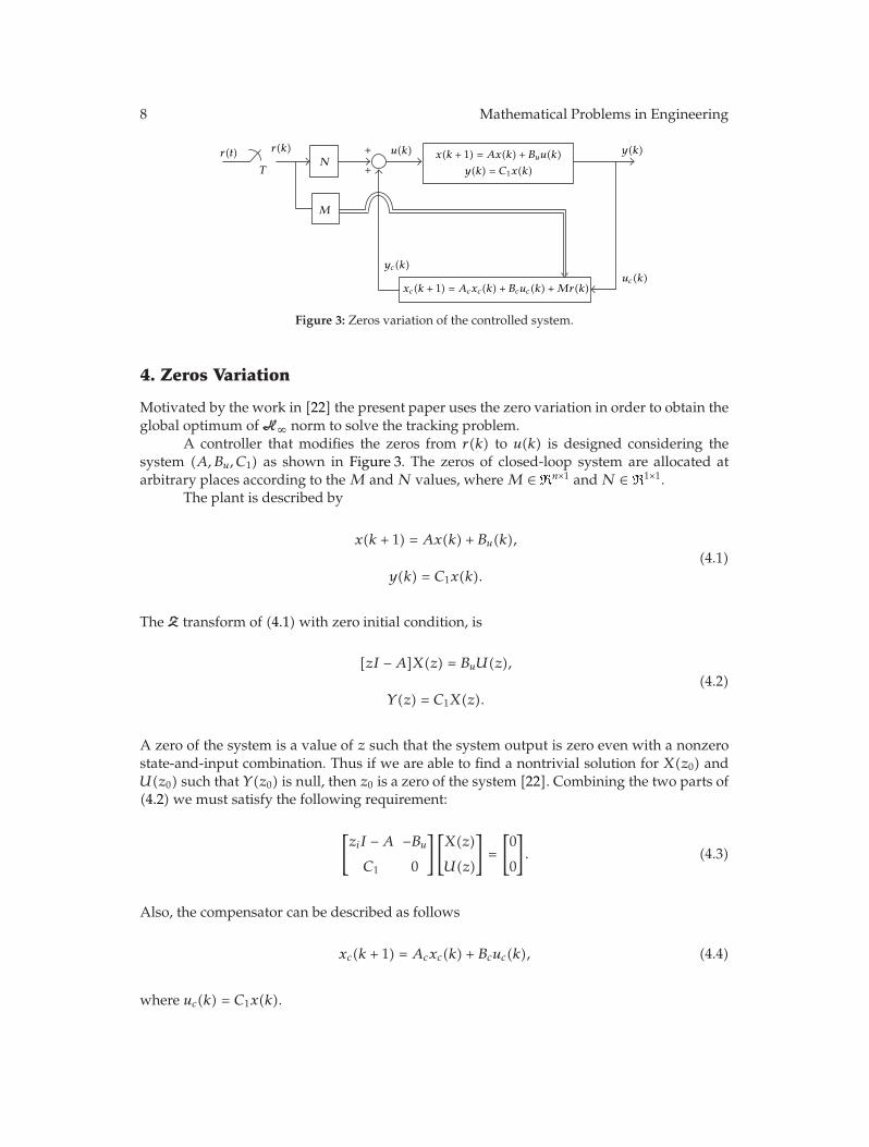
Figure 3: Zeros variation of the controlled system.
4. Zeros Variation
Motivated by the work in [22] the present paper uses the zero variation in order to obtain theglobal optimum of H∞ norm to solve the tracking problem.
A controller that modifies the zeros from r(k) to u(k) is designed considering thesystem (A,Bu, C1) as shown in Figure 3. The zeros of closed-loop system are allocated atarbitrary places according to theM andN values, whereM ∈ �n×1 andN ∈ �1×1.
The plant is described by
x(k + 1) = Ax(k) + Bu(k),
y(k) = C1x(k).(4.1)
The Z transform of (4.1) with zero initial condition, is
[zI −A]X(z) = BuU(z),
Y(z) = C1X(z).(4.2)
A zero of the system is a value of z such that the system output is zero even with a nonzerostate-and-input combination. Thus if we are able to find a nontrivial solution for X(z0) andU(z0) such that Y(z0) is null, then z0 is a zero of the system [22]. Combining the two parts of(4.2) we must satisfy the following requirement:
[ziI −A −BuC1 0
][X(z)
U(z)
]=
[0
0
]. (4.3)
Also, the compensator can be described as follows
xc(k + 1) = Acxc(k) + Bcuc(k), (4.4)
where uc(k) = C1x(k).
Mathematical Problems in Engineering 9
A more general method to introduce r(k) is to add a termMr(k) to xc(k + 1) and alsoa term Nr(k) to the control equation u(k) = Ccxc(k), as shown in Figure 3. The controller,with these additions, becomes equal to:
xc(k + 1) = Acxc(k) + Bcuc(k) +Mr(k),
u(k) = Ccxc(k) +Nr(k).(4.5)
Now, considering the controller (4.5), if there exists a transmission zero from r(k) to u(k),then necessarily there exists a transmission zero from r(k) to y(k), unless a pole of the plantcancels the zero. The equation to obtain zi from r(k) to u(k) (we let y(k) = 0 because we areconsidering only the effects of r(k), then uc(k) = 0) in (4.5), is the following:
[ziI −Ac −MCc N
][xco
ro
]=
[0
0
]. (4.6)
Because the coefficient matrix in (4.6) is square, the condition for a nontrivial solution is thatthe determinant of this matrix must be zero. Thus we have
det
[ziI −Ac −MCc N
]= 0. (4.7)
Multiplying the second column of the matrix described in (4.7) at right by a nonzero matrixN−1 and then adding to the first column of (4.7) the product of −Cc by the last column, wehave:
det
[ziI −Ac +MN−1Cc −MN−1
0 1
]= 0. (4.8)
And so, considering zi = z,
det(zI −Ac +MN−1Cc
)= 0, (4.9)
where the modified zeros from r(k) to u(k) are the solutions z = zi. It is important to noticethat the gain N and the vector M do not only modify the system zeros but also are used toobtain the optimal solution of the tracking problem.
5. Tracking Design
The solution of the tracking problem is based on the design of the matrices of the controllerM andN, that minimize the H∞ norm of (Am, Bm,−Cm, 1). Weighted frequency is added inthe tracking system in order to track signals in a frequency band specified in the design.
10 Mathematical Problems in Engineering
E(z)Hm(z)
Em(z) Ev(z)V (z)
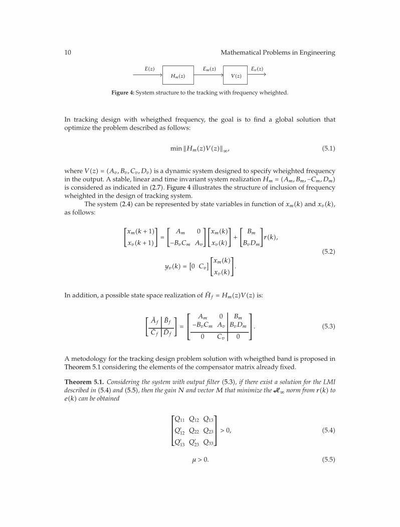
Figure 4: System structure to the tracking with frequency wheighted.
In tracking design with wheigthed frequency, the goal is to find a global solution thatoptimize the problem described as follows:
min ‖Hm(z)V (z)‖∞, (5.1)
where V (z) = (Av, Bv, Cv,Dv) is a dynamic system designed to specify wheighted frequencyin the output. A stable, linear and time invariant system realizationHm = (Am, Bm,−Cm,Dm)is considered as indicated in (2.7). Figure 4 illustrates the structure of inclusion of frequencywheighted in the design of tracking system.
The system (2.4) can be represented by state variables in function of xm(k) and xv(k),as follows:
[xm(k + 1)
xv(k + 1)
]=
[Am 0
−BvCm Av
][xm(k)
xv(k)
]+
[Bm
BvDm
]r(k),
yv(k) =[0 Cv
][xm(k)xv(k)
].
(5.2)
In addition, a possible state space realization of Hf = Hm(z)V (z) is:
[Af Bf
Cf Df
]=
⎡⎢⎣
Am 0 Bm−BvCm Av BvDm
0 Cv 0
⎤⎥⎦. (5.3)
A metodology for the tracking design problem solution with wheigthed band is proposed inTheorem 5.1 considering the elements of the compensator matrix already fixed.
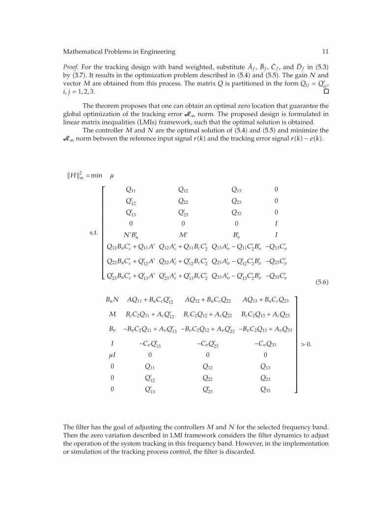
Theorem 5.1. Considering the system with output filter (5.3), if there exist a solution for the LMIdescribed in (5.4) and (5.5), then the gainN and vectorM that minimize theH∞ norm from r(k) toe(k) can be obtained
⎡⎢⎢⎣Q11 Q12 Q13
Q′12 Q22 Q23
Q′13 Q′
23 Q33
⎤⎥⎥⎦ > 0, (5.4)
μ > 0. (5.5)
Mathematical Problems in Engineering 11
Proof. For the tracking design with band weighted, substitute Af , Bf , Cf , and Df in (5.3)by (3.7). It results in the optimization problem described in (5.4) and (5.5). The gain N andvector M are obtained from this process. The matrix Q is partitioned in the form Qij = Q′
ij ,i, j = 1, 2, 3.
The theorem proposes that one can obtain an optimal zero location that guarantee theglobal optimization of the tracking error H∞ norm. The proposed design is formulated inlinear matrix inequalities (LMIs) framework, such that the optimal solution is obtained.
The controller M and N are the optimal solution of (5.4) and (5.5) and minimize theH∞ norm between the reference input signal r(k) and the tracking error signal r(k) − e(k).
‖H‖2∞ =min μ
s.t.
⎡⎢⎢⎢⎢⎢⎢⎢⎢⎢⎢⎢⎢⎢⎢⎢⎢⎢⎢⎢⎣
Q11 Q12 Q13 0
Q′12 Q22 Q23 0
Q′13 Q′
23 Q33 0
0 0 0 I
N ′B′u M′ B′
v I
Q12BuC′c +Q11A′ Q12A′
c +Q11BcC′2 Q13A′
v −Q11C′2B
′v −Q13C′
v
Q22BuC′c +Q
′12A
′ Q22A′c +Q
′12BcC
′2 Q23A
′v −Q′
12C′2B
′v −Q23C
′v
Q′23BuC
′c +Q
′13A
′ Q′23A
′c +Q
′13BcC
′2 Q33A′
v −Q′13C
′2B
′v −Q33C′
v
BuN AQ11 + BuCcQ′12 AQ12 + BuCcQ22 AQ13 + BuCcQ23
M BcC2Q11 +AcQ′12 BcC2Q12 +AcQ22 BcC2Q13 +AcQ23
Bv −BvC2Q11 +AvQ′13 −BvC2Q12 +AvQ
′23 −BvC2Q13 +AvQ33
I −CvQ′13 −CvQ
′23 −CvQ33
μI 0 0 0
0 Q11 Q12 Q13
0 Q′12 Q22 Q23
0 Q′13 Q′
23 Q33
⎤⎥⎥⎥⎥⎥⎥⎥⎥⎥⎥⎥⎥⎥⎥⎥⎥⎥⎥⎥⎥⎦
> 0.
(5.6)
The filter has the goal of adjusting the controllersM andN for the selected frequency band.Then the zero variation described in LMI framework considers the filter dynamics to adjustthe operation of the system tracking in this frequency band. However, in the implementationor simulation of the tracking process control, the filter is discarded.
12 Mathematical Problems in Engineering
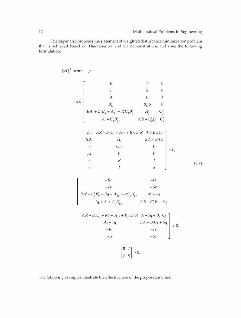
The paper also proposes the statement of weighted disturbance minimization problemthat is achieved based on Theorems 3.1 and 5.1 demonstrations and uses the followingformulation:
‖H‖2∞ =min μ
s.t.
⎡⎢⎢⎢⎢⎢⎢⎢⎢⎢⎢⎢⎢⎣
R I 0
I S 0
0 0 I
B′w B′
wS 0
RA′ +C′jB
′u +A
′fr + R
′C′1B
′fr A′
j C′fr
A′ + C′1B
′fr A′S + C′
2B′j C′
2
Bw AR + BuCj +Afr + BfrC1R A + BfrC1
SBw Aj SA + BjC2
0 Cfr 0
μI 0 0
0 R I
0 I S
⎤⎥⎥⎥⎥⎥⎥⎥⎥⎥⎥⎥⎦> 0,
⎡⎢⎢⎢⎢⎢⎢⎣
−Rr −Ir−Ir −Sr
RA′ + C′jB
′u + Rq +A
′fr + RC
′1B
′fr A′
j + Iq
Iq +A′ + C′1B
′fr A′S + C′
1B′j + Sq
AR + BuCj + Rq +Afr + BfrC1R A + Iq + BfrC1
Aj + Iq SA + BjC1 + Sq
−Rr −Ir−Ir −Sr
⎤⎥⎥⎥⎥⎥⎦ < 0,
[R I
I S
]> 0.
(5.7)
The following examples illustrate the effectiveness of the proposed method.
Mathematical Problems in Engineering 13
6. Example 1
Consider a tank temperature control system described in [22], with a zero-order hold. Thegoal is to design a tracking system for flow control with disturbance attenuation. The modelof the delayed system [22] is,
H(s) =e(−λ ∗ s)s
a+ 1
. (6.1)
A sampling period of 0.01 seconds is used in the design. The parameters a = 1 and λ = 0.005 sare adopted in the design.
We found λ = 1 ∗ 0.01 − 0.5 ∗ 0.01, and therefore, l = 1 andm = 0.5.Using the process to find the Z transform of a delayed continuous-time function (6.1),
the parameters are substituted and we obtain
H(z) =(1 − e−0.005
)z + (e−0.005 − e−0.01)/(1 − e−0.005)
z(z − e−0.01) , (6.2)
or,
H(z) =0.0050z + 0.0050z2 − 0.9900z
. (6.3)
The state-space description of the system is
[x1(k + 1)
x2(k + 1)
]=
[0.99 0
1 0
][x1(k)
x2(k)
]+
[1
0
]u(k) +
[1
0
]w(k),
y(k) =[0.005 0.005
][x1(k)x2(k)
],
(6.4)
where x(k) is the state vector, u(k) is the control signal and w(k) is a disturbance signal inthe system.
The design of the tracking system must include operation for reference signals of lowfrequencies (smaller than 0.1 rad/s). In such a case, the following filter J(z)was considered
J(z) =(0.4500z + 0.4500) × 10−7
z2 − 1.9999z − 0.9999. (6.5)
Using Theorem 3.1 the controller Kc(z) is designed for the system described in (6.4) andshowed in (6.6). This controller minimizes the H∞-norm of w(k) to z(k). In this design weobtain a disk of radius r = 0.5 and center in q = 0.5 is used as a pole placement constraint:
Kc(z) =−24.1395z− 4.6956z2 − 0.2981z + 0.1392
. (6.6)
14 Mathematical Problems in Engineering
10−2 10−1 100 101 1020.031
0.0315
0.032
0.0325
0.033
0.0335
0.034
0.0345
0.035
Mag
nitude
Frequency (rad/s)
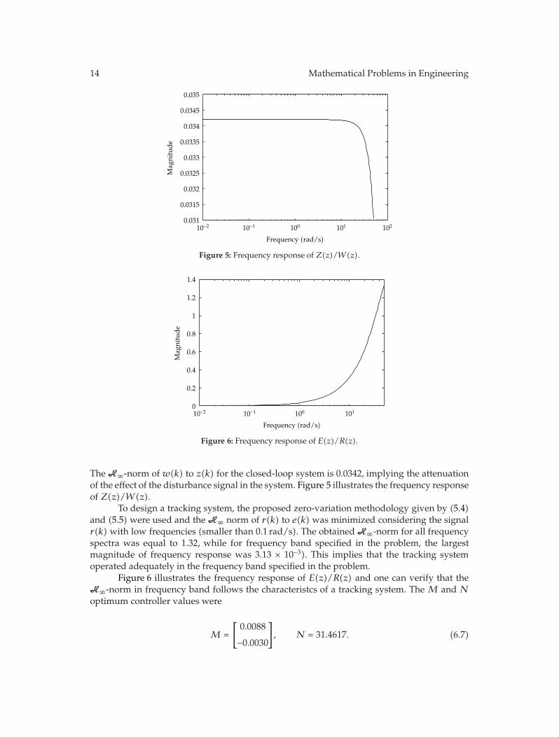
Figure 5: Frequency response of Z(z)/W(z).
10−2 10−1 100 101
Frequency (rad/s)
0
0.2
0.4
0.6
0.8
1
1.2
1.4
Mag
nitude
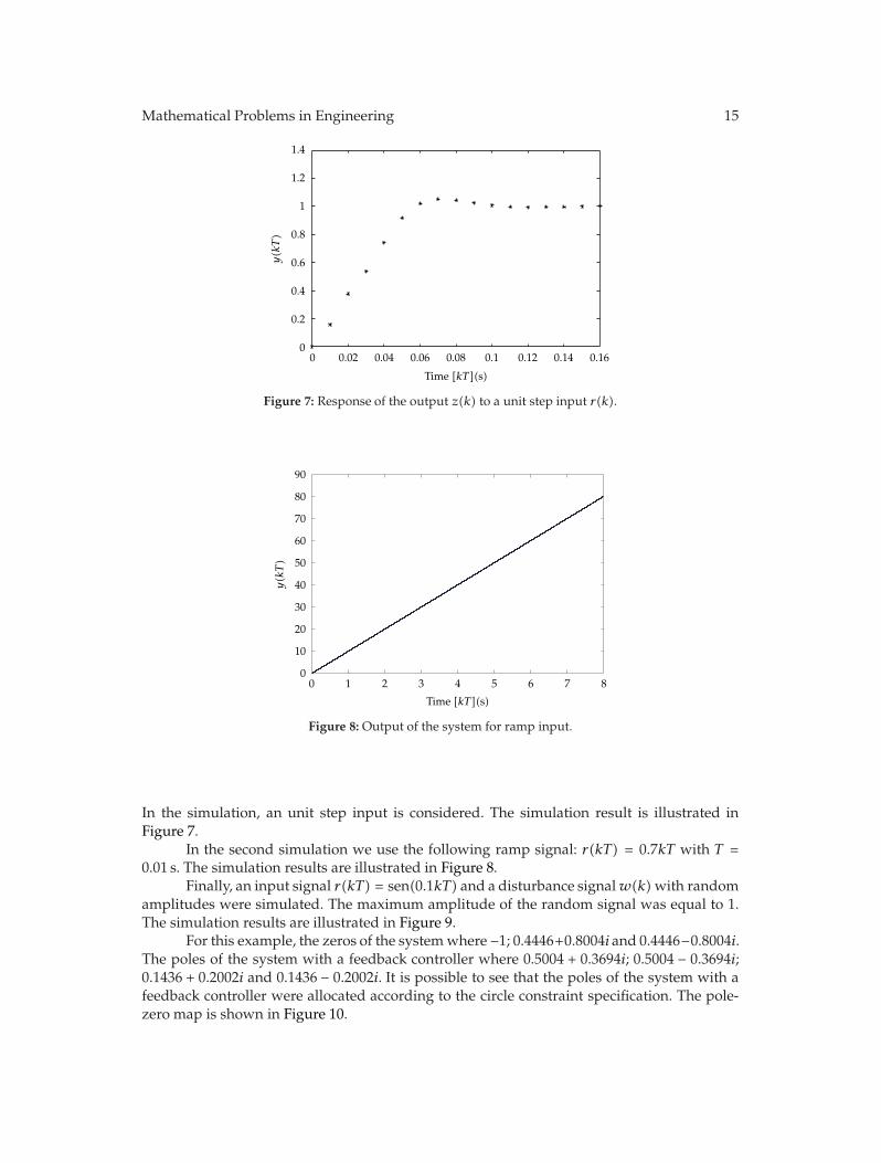
Figure 6: Frequency response of E(z)/R(z).
The H∞-norm of w(k) to z(k) for the closed-loop system is 0.0342, implying the attenuationof the effect of the disturbance signal in the system. Figure 5 illustrates the frequency responseof Z(z)/W(z).
To design a tracking system, the proposed zero-variation methodology given by (5.4)and (5.5) were used and the H∞ norm of r(k) to e(k) was minimized considering the signalr(k) with low frequencies (smaller than 0.1 rad/s). The obtained H∞-norm for all frequencyspectra was equal to 1.32, while for frequency band specified in the problem, the largestmagnitude of frequency response was 3.13 × 10⁻³). This implies that the tracking systemoperated adequately in the frequency band specified in the problem.
Figure 6 illustrates the frequency response of E(z)/R(z) and one can verify that theH∞-norm in frequency band follows the characteristcs of a tracking system. The M and Noptimum controller values were
M =
[0.0088
−0.0030
], N = 31.4617. (6.7)
Mathematical Problems in Engineering 15
0 0.02 0.04 0.06 0.08 0.1 0.12 0.14 0.160
0.2
0.4
0.6
0.8
1
1.2
1.4
Time [kT](s)
y(kT)
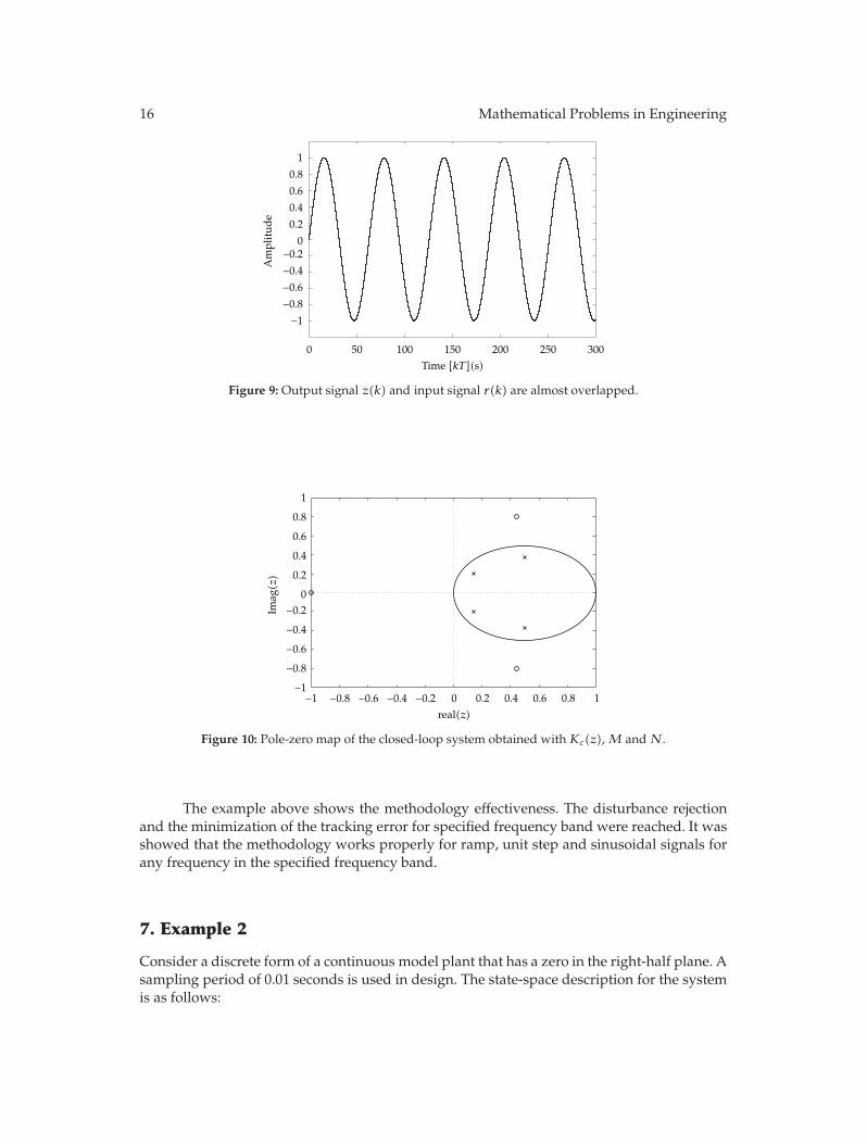
Figure 7: Response of the output z(k) to a unit step input r(k).
0 1 2 3 4 5 6 7 80
10
20
30
40
50
60
70
80
90
Time [kT](s)
y(kT)
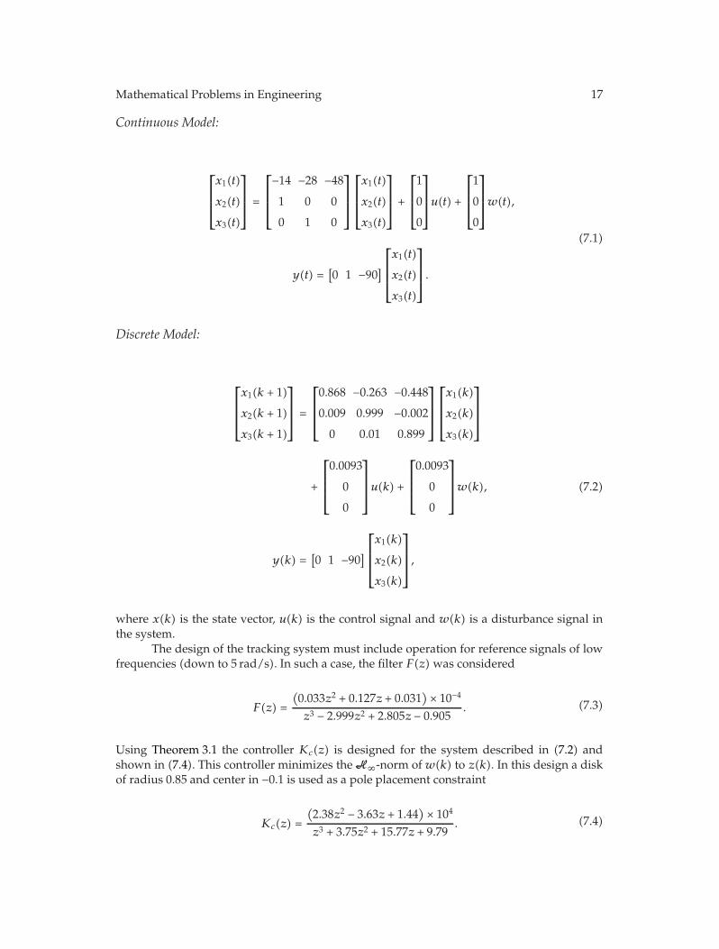
Figure 8: Output of the system for ramp input.
In the simulation, an unit step input is considered. The simulation result is illustrated inFigure 7.
In the second simulation we use the following ramp signal: r(kT) = 0.7kT with T =0.01 s. The simulation results are illustrated in Figure 8.
Finally, an input signal r(kT) = sen(0.1kT) and a disturbance signalw(k)with randomamplitudes were simulated. The maximum amplitude of the random signal was equal to 1.The simulation results are illustrated in Figure 9.
For this example, the zeros of the systemwhere −1; 0.4446+0.8004i and 0.4446−0.8004i.The poles of the system with a feedback controller where 0.5004 + 0.3694i; 0.5004 − 0.3694i;0.1436 + 0.2002i and 0.1436 − 0.2002i. It is possible to see that the poles of the system with afeedback controller were allocated according to the circle constraint specification. The pole-zero map is shown in Figure 10.
16 Mathematical Problems in Engineering
Time [kT](s)0 50 100 150 200 250 300
−1−0.8−0.6−0.4−0.2
0
0.2
0.4
0.6
0.8
1
Amplitud
e
Figure 9: Output signal z(k) and input signal r(k) are almost overlapped.
−1 −0.8 −0.6 −0.4 −0.2 0 0.2 0.4 0.6 0.8 1−1
−0.8−0.6−0.4−0.2
0
0.2
0.4
0.6
0.8
1
real(z)
Imag
(z)
Figure 10: Pole-zero map of the closed-loop system obtained withKc(z),M andN.
The example above shows the methodology effectiveness. The disturbance rejectionand the minimization of the tracking error for specified frequency band were reached. It wasshowed that the methodology works properly for ramp, unit step and sinusoidal signals forany frequency in the specified frequency band.
7. Example 2
Consider a discrete form of a continuous model plant that has a zero in the right-half plane. Asampling period of 0.01 seconds is used in design. The state-space description for the systemis as follows:
where x(k) is the state vector, u(k) is the control signal and w(k) is a disturbance signal inthe system.
The design of the tracking system must include operation for reference signals of lowfrequencies (down to 5 rad/s). In such a case, the filter F(z) was considered
F(z) =
(0.033z2 + 0.127z + 0.031
) × 10−4
z3 − 2.999z2 + 2.805z − 0.905. (7.3)
Using Theorem 3.1 the controller Kc(z) is designed for the system described in (7.2) andshown in (7.4). This controller minimizes the H∞-norm ofw(k) to z(k). In this design a diskof radius 0.85 and center in −0.1 is used as a pole placement constraint
Kc(z) =
(2.38z2 − 3.63z + 1.44
) × 104
z3 + 3.75z2 + 15.77z + 9.79. (7.4)
18 Mathematical Problems in Engineering
10−2 10−1 100 101
Frequency (rad/s)
1.54
1.545
1.55
1.555
1.56
1.565
1.57
1.575
1.58×10⁻³
Mag
nitude
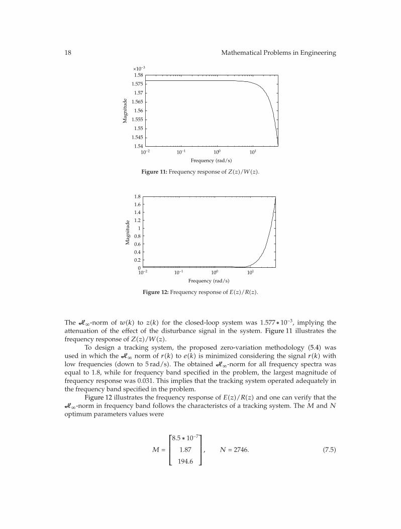
Figure 11: Frequency response of Z(z)/W(z).
10−2 10−1 100 101
Frequency (rad/s)
0
0.2
0.4
0.6
0.8
1
1.2
1.4
1.6
1.8
Mag
nitude
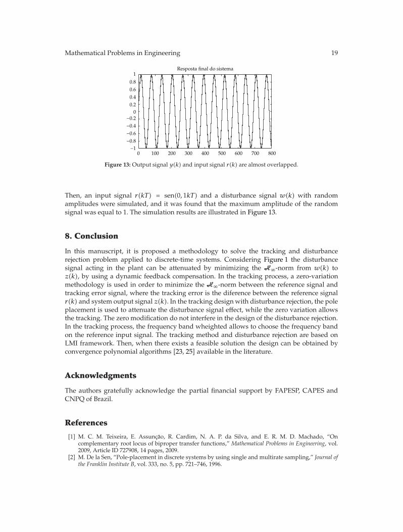
Figure 12: Frequency response of E(z)/R(z).
The H∞-norm of w(k) to z(k) for the closed-loop system was 1.577∗ 10−3, implying theattenuation of the effect of the disturbance signal in the system. Figure 11 illustrates thefrequency response of Z(z)/W(z).
To design a tracking system, the proposed zero-variation methodology (5.4) wasused in which the H∞ norm of r(k) to e(k) is minimized considering the signal r(k) withlow frequencies (down to 5 rad/s). The obtained H∞-norm for all frequency spectra wasequal to 1.8, while for frequency band specified in the problem, the largest magnitude offrequency response was 0.031. This implies that the tracking system operated adequately inthe frequency band specified in the problem.
Figure 12 illustrates the frequency response of E(z)/R(z) and one can verify that theH∞-norm in frequency band follows the characteristcs of a tracking system. The M and Noptimum parameters values were
M =
⎡⎢⎢⎣8.5 ∗ 10−7
1.87
194.6
⎤⎥⎥⎦, N = 2746. (7.5)
Mathematical Problems in Engineering 19
0 100 200 300 400 500 600 700 800−1
−0.8−0.6−0.4−0.2
00.20.40.60.8
1Resposta final do sistema
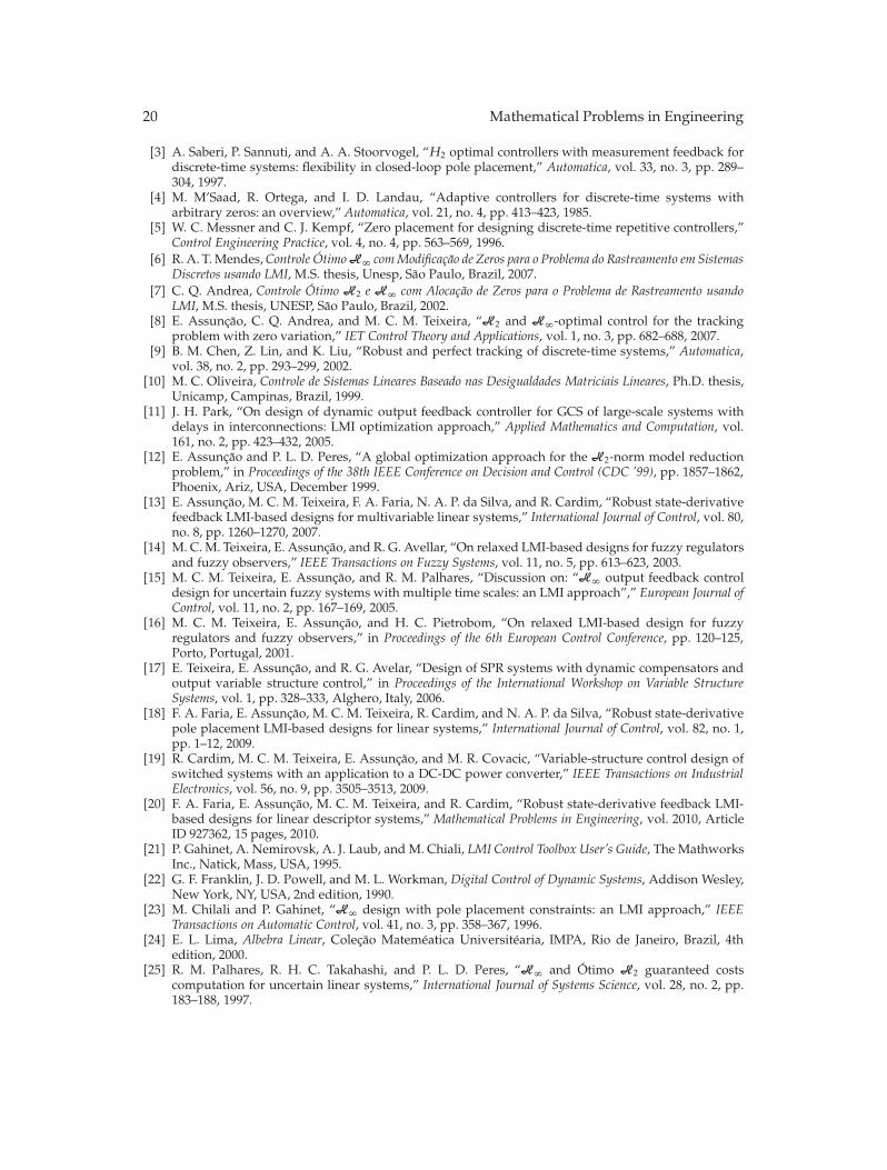
Figure 13: Output signal y(k) and input signal r(k) are almost overlapped.
Then, an input signal r(kT) = sen(0, 1kT) and a disturbance signal w(k) with randomamplitudes were simulated, and it was found that the maximum amplitude of the randomsignal was equal to 1. The simulation results are illustrated in Figure 13.
8. Conclusion
In this manuscript, it is proposed a methodology to solve the tracking and disturbancerejection problem applied to discrete-time systems. Considering Figure 1 the disturbancesignal acting in the plant can be attenuated by minimizing the H∞-norm from w(k) toz(k), by using a dynamic feedback compensation. In the tracking process, a zero-variationmethodology is used in order to minimize the H∞-norm between the reference signal andtracking error signal, where the tracking error is the diference between the reference signalr(k) and system output signal z(k). In the tracking designwith disturbance rejection, the poleplacement is used to attenuate the disturbance signal effect, while the zero variation allowsthe tracking. The zero modification do not interfere in the design of the disturbance rejection.In the tracking process, the frequency band wheighted allows to choose the frequency bandon the reference input signal. The tracking method and disturbance rejection are based onLMI framework. Then, when there exists a feasible solution the design can be obtained byconvergence polynomial algorithms [23, 25] available in the literature.
Acknowledgments
The authors gratefully acknowledge the partial financial support by FAPESP, CAPES andCNPQ of Brazil.
References
[1] M. C. M. Teixeira, E. Assuncao, R. Cardim, N. A. P. da Silva, and E. R. M. D. Machado, “Oncomplementary root locus of biproper transfer functions,” Mathematical Problems in Engineering, vol.2009, Article ID 727908, 14 pages, 2009.
[2] M. De la Sen, “Pole-placement in discrete systems by using single and multirate sampling,” Journal ofthe Franklin Institute B, vol. 333, no. 5, pp. 721–746, 1996.
20 Mathematical Problems in Engineering
[3] A. Saberi, P. Sannuti, and A. A. Stoorvogel, “H2 optimal controllers with measurement feedback fordiscrete-time systems: flexibility in closed-loop pole placement,” Automatica, vol. 33, no. 3, pp. 289–304, 1997.
[4] M. M’Saad, R. Ortega, and I. D. Landau, “Adaptive controllers for discrete-time systems witharbitrary zeros: an overview,” Automatica, vol. 21, no. 4, pp. 413–423, 1985.
[5] W. C. Messner and C. J. Kempf, “Zero placement for designing discrete-time repetitive controllers,”Control Engineering Practice, vol. 4, no. 4, pp. 563–569, 1996.
[6] R. A. T.Mendes,Controle OtimoH∞ comModificacao de Zeros para o Problema do Rastreamento em SistemasDiscretos usando LMI, M.S. thesis, Unesp, Sao Paulo, Brazil, 2007.
[7] C. Q. Andrea, Controle Otimo H2 e H∞ com Alocacao de Zeros para o Problema de Rastreamento usandoLMI, M.S. thesis, UNESP, Sao Paulo, Brazil, 2002.
[8] E. Assuncao, C. Q. Andrea, and M. C. M. Teixeira, “H2 and H∞-optimal control for the trackingproblem with zero variation,” IET Control Theory and Applications, vol. 1, no. 3, pp. 682–688, 2007.
[9] B. M. Chen, Z. Lin, and K. Liu, “Robust and perfect tracking of discrete-time systems,” Automatica,vol. 38, no. 2, pp. 293–299, 2002.
[10] M. C. Oliveira, Controle de Sistemas Lineares Baseado nas Desigualdades Matriciais Lineares, Ph.D. thesis,Unicamp, Campinas, Brazil, 1999.
[11] J. H. Park, “On design of dynamic output feedback controller for GCS of large-scale systems withdelays in interconnections: LMI optimization approach,” Applied Mathematics and Computation, vol.161, no. 2, pp. 423–432, 2005.
[12] E. Assuncao and P. L. D. Peres, “A global optimization approach for the H2-norm model reductionproblem,” in Proceedings of the 38th IEEE Conference on Decision and Control (CDC ’99), pp. 1857–1862,Phoenix, Ariz, USA, December 1999.
[13] E. Assuncao, M. C. M. Teixeira, F. A. Faria, N. A. P. da Silva, and R. Cardim, “Robust state-derivativefeedback LMI-based designs for multivariable linear systems,” International Journal of Control, vol. 80,no. 8, pp. 1260–1270, 2007.
[14] M. C.M. Teixeira, E. Assuncao, and R. G. Avellar, “On relaxed LMI-based designs for fuzzy regulatorsand fuzzy observers,” IEEE Transactions on Fuzzy Systems, vol. 11, no. 5, pp. 613–623, 2003.
[15] M. C. M. Teixeira, E. Assuncao, and R. M. Palhares, “Discussion on: “H∞ output feedback controldesign for uncertain fuzzy systems with multiple time scales: an LMI approach”,” European Journal ofControl, vol. 11, no. 2, pp. 167–169, 2005.
[16] M. C. M. Teixeira, E. Assuncao, and H. C. Pietrobom, “On relaxed LMI-based design for fuzzyregulators and fuzzy observers,” in Proceedings of the 6th European Control Conference, pp. 120–125,Porto, Portugal, 2001.
[17] E. Teixeira, E. Assuncao, and R. G. Avelar, “Design of SPR systems with dynamic compensators andoutput variable structure control,” in Proceedings of the International Workshop on Variable StructureSystems, vol. 1, pp. 328–333, Alghero, Italy, 2006.
[18] F. A. Faria, E. Assuncao, M. C. M. Teixeira, R. Cardim, and N. A. P. da Silva, “Robust state-derivativepole placement LMI-based designs for linear systems,” International Journal of Control, vol. 82, no. 1,pp. 1–12, 2009.
[19] R. Cardim, M. C. M. Teixeira, E. Assuncao, and M. R. Covacic, “Variable-structure control design ofswitched systems with an application to a DC-DC power converter,” IEEE Transactions on IndustrialElectronics, vol. 56, no. 9, pp. 3505–3513, 2009.
[20] F. A. Faria, E. Assuncao, M. C. M. Teixeira, and R. Cardim, “Robust state-derivative feedback LMI-based designs for linear descriptor systems,” Mathematical Problems in Engineering, vol. 2010, ArticleID 927362, 15 pages, 2010.
[21] P. Gahinet, A. Nemirovsk, A. J. Laub, and M. Chiali, LMI Control Toolbox User’s Guide, The MathworksInc., Natick, Mass, USA, 1995.
[22] G. F. Franklin, J. D. Powell, and M. L. Workman, Digital Control of Dynamic Systems, Addison Wesley,New York, NY, USA, 2nd edition, 1990.
[23] M. Chilali and P. Gahinet, “H∞ design with pole placement constraints: an LMI approach,” IEEETransactions on Automatic Control, vol. 41, no. 3, pp. 358–367, 1996.
[24] E. L. Lima, Albebra Linear, Colecao Matemeatica Universitearia, IMPA, Rio de Janeiro, Brazil, 4thedition, 2000.
[25] R. M. Palhares, R. H. C. Takahashi, and P. L. D. Peres, “H∞ and Otimo H2 guaranteed costscomputation for uncertain linear systems,” International Journal of Systems Science, vol. 28, no. 2, pp.183–188, 1997.