East Palatka_Nitrogen Modeling_Report

Estimation of Nitrogen Load from Septic

Systems to Surface Waterbodies in East

Palatka, Putnam County, FL.

Manuscript Completed: October, 2014

Prepared by

Mohammad Sayemuzzaman and Ming Ye

Department of Scientific Computing, Florida State University,

Tallahassee, FL 32306

Rick Hicks, FDEP Contract Manager

Prepared for

Florida Department of Environmental Protection

Tallahassee, FL

Estimation of Nitrogen Load for East Palatka, Putnam County, FL.

i

EXECUTIVE SUMMARY

The ArcGIS-based Nitrate Load Estimation Toolkit (ArcNLET), which was developed for the

Florida Department of Environmental Protection (FDEP) by the Florida State University

(FSU), was used in this study for East Palatka in Putnam County, FL. The purpose of this

project is to estimate the reduction of nitrogen load from 158 septic systems to the St. Johns

River and other surface waterbodies in the town. While ArcNLET is based on a simplified

model of groundwater flow and nitrogen transport, the model considers heterogeneous

hydraulic conductivity and porosity as well as spatial variability of septic system locations,

surface water bodies, and distances between septic systems and surface water bodies.

ArcNLET also considers key mechanisms controlling nitrogen transport, including advection,

dispersion, and denitrification. After preparing model input files in the ArcGIS format, setting

up an ArcNLET model run is easy through a graphic user interface. The modeling results are

readily available for post-processing and visualization within ArcGIS. The modeling results

include Darcy velocity, groundwater flow paths from septic systems to surface water bodies,

spatial distribution of nitrogen plumes, and nitrogen load estimates to individual surface water

bodies; these results can be used directly for environmental management and regulation of

nitrogen pollution. The ArcNLET flow and transport models of this study were established

using data downloaded from public-domain websites and provided by colleagues from FDEP.

Due to the lack of observations of hydraulic head and nitrogen concentration in the modeling

area, model calibration was not conducted in this study. Site-specific data of DEM,

waterbodies, septic locations, hydraulic conductivity, and porosity were used in the ArcNLET

modeling. The ArcGIS layer of surface waterbodies was updated to include small waterbodies

that are missing in the layer but reflected in the DEM layer. Literature-based parameter values

were used for smoothing factor in the flow modeling, and for longitudinal dispersivity (𝛼𝐿),

transverse horizontal dispersivity (𝛼𝑇), decay coefficient (k), inflow mass to groundwater (Min),

and source plane concentration (C0) in the transport modeling. Due to uncertainty in the

literature-based parameter values of dispersivities (𝛼𝐿 and 𝛼𝑇) and denitrification coefficient

(k), four cases with four sets of the parameters were considered, and their values are listed in

Table ES-1 together with the literature-based values of the other three parameters. Cases 1 and

2 considered two sets of 𝛼𝐿 and 𝛼𝑇 values, and Cases 3 and 4 used a different k value. The

justification of using these values is given in the text.

Table ES-1. Literature based values of ArcNLET model parameters.

Parameter Case 1 Case 2 Case 3 Case 4

Smoothing factor 60 60 60 60

Min (g/d) 19.84 19.84 19.84 19.84

C0 (mg/L) 40 40 40 40

𝛼𝐿 (m) 2.134 6 2.134 6

𝛼𝑇 (m) 0.0549 2.5 0.0549 2.5

k (d-1) 0.011 0.011 0.001 0.001

Figure ES-1 plots the simulated flow paths from the individual septic systems to the surface

waterbodies. The St. Johns River (waterbody 23 and waterbody 21), has the largest number

(106) of contributing septic systems. Waterbdy 4 has the second largest number (20) of


ii

contributing septic systems. Waterbody 8 has the third largest number (18) of contributing

septic systems.

Figure ES-1. Waterbodies FID, Septic tank locations and the particle flow paths

Table ES-2 lists for the four cases the ArcNLET-estimated total loads (in the units of g/d and

lb/yr) from the 158 septic systems, load (g/d) per septic system, reduction ratios (%), load (g/d)

to the St. Johns River, and the percent of the total loads that the St. Johns River receives. The

reduction ratio is the amount of denitrified nitrogen (i.e., the difference between the load to

groundwater and the load to surface waterbodies) divided by the load to groundwater (i.e., the

inflow mass, Min, listed in Table ES-1). This table shows that the load estimate depends more

on the denitrification coefficient than on the dispersivities. For example, Cases 1 and 3 have

the same dispersivities (αL = 2.134 m, αT = 0.0549 m) but different denitrification coefficients

(0.011 d-1 for Case 1 and 0.001 d-1 for Case 3). The two cases have dramatically different load

estimates, with the estimate of Case 3 being 2.96 times as large as that of Case 1. The ratio is

2.85 between the estimates of Cases 4 and 2, when the dispersivities change to another set (αL

= 6 m and αT = 2.5 m). The reduction ratio changes from 78% (case 1) and 77% (case 2) to

36% (case 3) and 36% (case 4), when the denitrification coefficient decreases from 0.011 d-1

to 0.001 d-1. These reduction ratios are comparable with those reported in literature, as

discussed in Ye and Sun (2013).

Figure ES-2 plots the estimated nitrogen loads to the eight waterbodies (with FIDs of 23, 8, 21,

4, 24, 25, 6, and 15) that receive all the nitrogen loads from the septic systems. For all the four

modeling cases, the St. Johns River (FID 23) and swamp (FID 21) adjacent to the St. Johns

River, receives the largest amount of load, about 80% of the total load. The percentage of total


iii

load is smaller in Cases 3 and 4 than in Cases 1 and 2. This may be attributed to the joint effects

of dispersivities and denitrification coefficient on the load estimate.

Table ES- 2. Simulated nitrogen loads to surface waterbodies and nitrogen reduction ratios for

158 septic systems in East Palatka.

Figure ES-2. Nitrogen loading (g/d) to the individual waterbodies for the four modeling

cases.

23 8 21 4 24 25 15 6 Total

Case 1 491 79 44 30 2 0.61 0.25 0.00 647

Case 2 509 82 48 33 2 0.67 0.25 0.00 675

Case 3 1262 183 185 214 45 16 10 2 1917

Case 4 1266 184 186 216 45 17 10 3 1927

0

200

400

600

800

1000

1200

1400

1600

1800

Nit

rate

load

(g/d

)

Total load

(g/d)

Total load

(lb/yr)

Load per septic

systems (g/d)

Reduction

ratio (%)

Load to

St. Johns

River

(g/d)

Percentage

of total load

to St. Johns

River

Case 1 647 521 4.10 78 536 83

Case 2 675 544 4.28 77 557 82

Case 3 1917 1543 12.13 36 1447 75

Case 4 1927 1551 12.20 36 1452 75


iv

The ArcNLET modeling of this study leads to the following major conclusions:

(1) The data and information needed to establish ArcNLET models for groundwater

modeling and nitrogen load estimation are readily available in the East Palatka. The

data are available in either the public domain (e.g., USGS websites) or FDEP database.

Site-specific data include DEM, waterbodies, septic locations, hydraulic conductivity,

and porosity. The values of smoothing factor, dispersivity, denitrification coefficient,

inflow mass to groundwater, and source plane concentration are obtained from

literature.

(2) Among the 158 septic systems, 106 septic systems contribute nitrogen load to the St.

Johns River. The rest of septic systems contribute nitrogen load to waterbodies that are

not connected to the St. Johns River. As a result, not all the future remove septic

systems will contribute to nitrogen load reduction in the TMDL practice. This suggests

importance of considering spatial variability in environmental management of nitrogen

contamination.

(3) For all the four modeling cases considered in this study, the load estimate to the St.

Johns River (combined of FID 23 and FID 21) is the largest, with the load ranging from

75% to 83% of the total load.

(4) The denitrification coefficient is the most influential parameter to the load estimate.

More effort should be spent to determine appropriate value of the parameter for more

accurate estimation of load reduction.


v

CONTENTS

EXECUTIVE SUMMARY ................................................................................................. i

1. INTRODUCTION .........................................................................................................1

2. SIMPLIFIED CONCEPTUAL MODEL OF ArcNLET................................................2

3. ARCNLET MODELING FOR EAST PALATKA (Lower St. Johns) ..........................7

3.1. Modeling Area and ArcGIS Input Data ............................................................ 7

3.2. Groundwater Flow Parameters ....................................................................... 10

3.3. Nitrogen Transport Parameters ....................................................................... 13

3.4. Nitrogen Load to Groundwater ....................................................................... 13

4. RESULTS AND DISCUSSION ..................................................................................15

4.1. Results of Groundwater Flow Modeling......................................................... 15

4.2. Nitrogen Transport Modeling Results ............................................................ 15

5. CONCLUSION ............................................................................................................22

6. REFERENCES ............................................................................................................23

APPENDIX A ....................................................................................................................27


vi

LIST OF FIGURES

Figure ES-1. Waterbodies FID, Septic tank locations and the particle flow paths.................. ii

Figure ES-2. Nitrogen loading (g/d) to the individual waterbodies for the four modeling cases.

.................................................................................................................................................. iii

Figure 2-1. Conceptual model of nitrate transport in groundwater adapted from Aziz et al.

(2000). The unsaturated zone is bounded by the rectangular box delineated by the dotted lines;

the groundwater zone is bounded by the box delineated by the solid lines .............................. 4

Figure 2-2. Main Graphic User Interface (GUI) of ArcNLET with four modules of

Groundwater Flow, Particle Tracking, Transport, and Denitrification. .................................... 6

Figure 3-1. Locations of septic systems (red dot) and modeling area delineated in the red

boundary. .................................................................................................................................. 7

Figure 3-2. Locations of waterbodies (red rectangular marked the modeling area) ................ 8

Figure 3-3. DEM data of the modeling area with the resolution of 3m × 3m. The black oval

delineate the areas where the layer of water body (Figures 3-2) needs to be updated to include

the missing pond/lake, swamp/marsh and part of river. ........................................................... 9

Figure 3-4. Google Earth image for part of the modeling area. The black oval mark from the

left represents part of river, swamp, and pond/lake consecutively, which reflected in the DEM

(Figure 3-3) but not shown in the layer of surface waterbodies (Figure 3-2). .......................... 9

Figure 3-5. Updated waterbodies map based on DEM and Google Earth. The waterbodies are

labeled by their FIDs; the FID of the added small channel of river is 23, ponds are 24 and 15,

and the FIDs of the added swamp/marsh is 25. ...................................................................... 10

Figure 3-6. Heterogeneous hydraulic conductivity (m/d) of soil units. ................................. 11

Figure 3-7. Heterogeneous porosity ([-]) of soil units. ......................................................... 12

Figure 4- 1 Simulated flow paths from septic systems to surface waterbodies. .................... 15

Figure 4- 2 Simulated flow paths from septic systems to surface waterbodies. Paramter values

specific to Case 1 are αL = 2.134 m, αT = 0.0549 m, and k = 0.011 d-1. .............................. 17

Figure 4- 3 Simulated flow paths from septic systems to surface waterbodies. Parameter values

specific to Case 2 are αL = 6 m, αT = 2.5 m, and k = 0.011 d-1. ........................................... 18


specific to Case 3 are αL = 2.134 m, αT = 0.0549 m, and k = 0.001 d-1. .............................. 19


specific to Case 4 are αL = 6 m, αT = 2.5 m, and k = 0.001 d-1. ........................................... 20

Figure 4- 6 Nitrogen loading (kg/d) to the individual waterbodies for the four modeling cases.

.................................................................................................. Error! Bookmark not defined.


vii

LIST OF TABLES

Table ES- 1 Literature-based values of ArcNLET model parameters. ..................................... i

Table ES- 2 Simulated nitrogen loads to surface waterbodies and nitrogen reduction ratios for

125 septic systems in East Palatka. .......................................................................................... iii

Table 3- 1 Literature-based values of ArcNLET model parameters. ..................................... 14

Table 4-1．Simulated nitrogen loads to surface waterbodies and groundwater (inflow mass)

for Case 1. Locations of the waterbodies are shown in Figure 4-2. ........................................ 17



Table 4-3. Simulated nitrogen loads to surface waterbodies and groundwater (inflow mass) for

Case 3. Locations of the waterbodies are shown in Figure 4-4. ............................................. 19



Table 4-5．Simulated nitrogen loads to surface waterbodies and nitrogen reduction ratios for

the four cases。....................................................................................................................... 21


1

1. INTRODUCTION

This report summarizes the modeling effort of the Florida State University (FSU) to support

management of nutrient pollution of the Florida Department of Environmental Protection

(FDEP) for the East Palatka. The location of East Palatka and the septic system locations

(provided by Richard Hicks, FDEP) are shown in Figure 1-1. The ArcGIS-Based Nitrate Load

Estimation Toolkit (ArcNLET) (Rios et al. 2013a; Wang et al., 2013), developed by FSU, is

used in this study to simulate groundwater flow and nitrate transport from septic systems in

surficial aquifers. With the assumption that ammonium transports in the same way as nitrate

does, ArcNLET can be used to simulate nitrogen fate and transport. ArcNLET provides the

following outputs:

(1) Approximation of water table shape in the modeling domain,

(2) Magnitude and direction of Darcy velocity at raster cells of the modeling domain,

(3) Nitrogen plumes from individual septic systems to nearby water bodies, and

(4) Nitrogen load estimates to the individual water bodies.

ArcNLET modeling requires the following ArcGIS raster and polygon files that are available

in the public domain:

(1) Digital elevation model (DEM) of topography that is available at the USGS National

Map Viewer and Download Framework (http://nationalmap.gov/viewer.html). The

DEM data is smoothed to generate the shape of water table, based on the assumption

that water table is a subdued replica of topography. The smoothed DEM is used to

evaluate groundwater flow magnitude and direction by using the Darcy’s law.

(2) Water body locations that are available from USGS National Hydrography Database

(http://nhd.usgs.gov/). Flow paths evaluated from the Darcy velocity vector from septic

systems are terminated at the water bodies.

(3) Locations of septic systems that are available in the database of Florida Department of

Health. For this study, the locations are provided by Richard W. Hicks at FDEP.

(4) Hydraulic conductivity and porosity of the modeling domain are available from the

Soil Survey Geographic Database (SSURGO) (http://websoilsurvey.nrcs.usda.gov).

The data above are site specific. ArcNLET modeling also involves the following parameters

of groundwater flow and solute transport that are obtained from model calibration and/or

literature:

(1) Dispersivities in the longitudinal and horizontal transverse directions,

(2) Inflow nitrogen mass from drainfields to groundwater,

(3) Nitrogen concentration in the effluent entering groundwater, and

(4) Decay coefficient of denitrification.

Site-specific values of these parameters can be obtained by model calibration, in which the

literature-based parameter values are adjusted to match the numerical simulations of hydraulic

head and nitrogen concentration to corresponding field observations. However, due to the lack

of field observations in this study, model calibration was not performed. Instead, the ArcNLET

simulation of this study is conducted using the parameter values obtained from literature and

our pervious modeling experience, e.g., the Julington Creek neighborhood in the City of

Jacksonville. Justification of using the parameter values is given Section 3.

http://nationalmap.gov/viewer.html

http://nhd.usgs.gov/

http://websoilsurvey.nrcs.usda.gov/


2

In the remainder of this report, the conceptual model of groundwater flow and nitrogen

transport used in ArcNLET and its computational implementation are briefly described in

Section 2. Sections 3 and 4 present the modeling practice and results for the East Palatka. The

summary and conclusions of this study are discussed in Section 5.

2. SIMPLIFIED CONCEPTUAL MODEL OF ArcNLET

ArcNLET is based on a simplified conceptual model of groundwater flow and nitrate transport.

The model has three sub-models: groundwater flow model, nitrate transport model, and nitrate

load estimation model. The results from the flow model are used by the transport model, whose

results are in turn utilized by the nitrate load estimation model. By invoking assumptions and

simplifications to the system being modeled, computational cost is significantly reduced,

which enables ArcNLET to provide quick estimates of nitrate loads from septic systems to

surface water bodies. The three submodels are briefly described here; more details of them can

be found in Rios (2010) and Rios et al. (2013a). Ammonium is not explicitly simulated in

ArcNLET. Instead, it is assumed in this study that ammonium transport is the same as nitrate

transport so that ArcNLET can simulate nitrogen transport and estimate nitrogen load, not

merely nitrate load, from septic systems to surface water bodies. This assumption however

may overestimate nitrogen loads.

The groundwater flow model of ArcNLET is simplified by assuming that the water table is a

subdued replica of the topography in the surficial aquifer. According to Haitjema and Mitchell-

Bruker (2005), the assumption is valid if

2

1RL

mKHd , (1)

where R [m/day] is recharge, L [m] is average distance between surface waters, m is a

dimensionless factor accounting for the aquifer geometry, and is between 8 and 16 for aquifers

that are strip-like or circular in shape, K [m/day] is hydraulic conductivity, H [m] is average

aquifer thickness, and d [m] is the maximum distance between the average water level in

surface water bodies and the elevation of the terrain. The criterion, as a rule of thumb, can be

met in shallow aquifers in flat or gently rolling terrain. Based on the assumption, the shape of

water table can be obtained by smoothing land surface topography given by DEM of the study

area. In ArcNLET, the smoothing is accomplished using moving-window average via a 7 × 7

averaging window. The smoothing process needs to be repeated for multiple times, depending

on discrepancy between the shapes of topography and water table. The number of the

smoothing process, called smoothing factor, is specified by ArcNLET users as an input

parameter of ArcNLET. This parameter needs to be calibrated against measured hydraulic

heads in the study area, as explained in detail in Section 4.

With the assumption that smoothed DEM has the same shape (not the same elevation) of water

table, hydraulic gradients can be estimated from the smoothed DEM. Subsequently,

groundwater seepage velocity, v, can be obtained by applying Darcy’s Law


3

x

y

K h K zv

x x

K h K zv

y y

, (2)

where K is hydraulic conductivity [LT-1], is porosity, h is hydraulic head, and hydraulic

gradient (∂h/∂x and ∂h/∂y) is approximated by the gradient of the smoothed topography (∂z/∂x

and ∂z/∂y). Implementing the groundwater flow model in the GIS environment yields the

magnitude and direction of the flow velocity for every discrete cell of the modeling domain,

which are used to estimate flow paths originating from individual septic systems and ending

in surface water bodies. The calculation considers spatial variability of hydraulic conductivity,

porosity, hydraulic head, and septic system locations. Because hydraulic gradients and water

bodies are not hydraulically linked in the model, ArcNLET users need to evaluate whether the

resulting shape of the water table is consistent with the drainage network associated the water

bodies. The values of hydraulic conductivity and conductivity can be obtained from field

measurements, literature data, and/or by calibration against measurements of hydraulic head

and groundwater velocity.

Additional assumptions and approximations of the flow model are made as follows: (1) the

Dupuit-Forchheimer assumption is used so that the vertical flow can be ignored and only two-

dimensional (2-D) isotropic horizontal flow is simulated; (2) the steady-state flow condition is

assumed, since this software is used for the purpose of long-term environmental planning; (3)

the surficial aquifer does not include karsts or conduits so that Darcy’s Law can be used; (4)

mounding on water table due to recharge from septic systems and rainfall is not explicitly

considered (but assumed to be reflected by the steady-state water table); (5) the flow field is

obtained from the water table without explicit consideration of a water balance; (6)

groundwater recharge from the estuary is disregarded. While these assumptions may not be

ideal, especially the assumption of steady-state, they are needed to make model complexity

compatible with available data and information and to make the model run efficient in the GIS

modeling environment.

Figure 2-1 shows the conceptual model of nitrate transport in ArcNLET, which is similar to

that of BIOSCREEN (Newell et al. 1996) and BIOCHLOR (Aziz et al. 2000) developed by

the U.S. EPA. In the conceptual model, nitrate enters the groundwater zone with a uniform and

steady flow in the direction indicated. The Y−Z plane in Figure 2-1 is considered as a source

plane (with a constant concentration C0 [ML-3]) through which nitrate enters the groundwater

system. Two-dimensional (2-D) nitrate transport in groundwater is described using the

advection-dispersion equation


4

Figure 2-1. Conceptual model of nitrate transport in groundwater adapted from Aziz et

al. (2000). The unsaturated zone is bounded by the rectangular box delineated by the

dotted lines; the groundwater zone is bounded by the box delineated by the solid lines

2 2

2 2x y

C C C CD D v kC

t x y x

(3)

where C is the nitrate concentration [M/L3], t is time [T], Dx and Dy are the dispersion

coefficients in the x and y directions, respectively [L2T−1], v is the constant seepage velocity in

the longitudinal direction [L], and k is the first-order decay coefficient [T−1]. This equation

assumes homogeneity of parameters (e.g., dispersion coefficient) and uniform flow in the

longitudinal direction. The last term in Eq. 3 is to simulate the denitrification, in which nitrate

is transformed into nitrogen gas through a series of biogeochemical reactions. Following

McCray et al. (2005) and Heinen (2006), the denitrification process is modeled using first-

order kinetics and included as the decay term, which can also be used to take into account other

loss processes. The steady-state form, semi-analytical solution of Eq. 3 is derived based on that

of West et al. (2007), which is of 3-D, steady-state form and similar to the work of Domenico

(1987). The analytical solution used in this study is (Rios, 2010; Rios et al., 2013a)

01 2

1

2

, ,2

4exp 1 1

2

/ 2 / 2

2 2

x

x

y y

CC x y F x F y x

kxF

v

y Y y YF erf erf

x x

(4)

where αx and αy [L] are longitudinal and horizontal transverse dispersivity, respectively, Y [L]

is the width of the source plane, and C0 [M/L3] is the constant source concentration at the

source plane. A review of analytical solutions of this kind and errors due to assumptions

involved in their derivation is provided by Srinivasan et al. (2007).

The 2-D concentration plume is extended downwards to the depth Z of the source plane Figure

2-1; the pseudo three-dimensional (3-D) plume is the basis for estimating the amount of nitrate

that enters into groundwater and loads to surface water bodies. While each individual septic

system has its own source concentration, C0, drainfield width, Y, and average plume thickness,

Z, the information and data of these variables are always unavailable in a management project.


5

Therefore, constant values are used for all septic systems in this study. ArcNLET allows using

different C0 values for different septic systems, if the data are available. Despite of the constant

values used for all the septic systems, each individual septic system has its own concentration

plume, because flow velocity varies between the septic systems. Since the flow velocity

estimated in the groundwater flow model is not uniform but varies in space, in order to use the

analytical solution with uniform velocity, the harmonic mean of velocity (averaged along the

flow path of a plume) is used for evaluating each individual plume. The plumes either end at

surface water bodies or are truncated at a threshold concentration value (usually very small,

e.g., 10-6). After the plumes for all septic systems are estimated, by virtue of linearity of the

advection-dispersion equation with respect to concentration, the individual plumes are added

together to obtain the spatial distribution of nitrate concentration in the modeling domain. The

superposition however may result in higher and shallower concentrations than exist in the field

unless the averaging depth is deep enough.

The nitrate load estimation model evaluates the amount of nitrate loaded to target surface water

bodies. For the steady-state model, this is done using the mass balance equation,

out in dnM M M , where outM [MT-1] is mass load rate to surface water bodies, inM [MT-1] is

mass inflow rate from septic systems to groundwater, and dnM [MT-1] is mass removal rate

due to denitrification. The mass inflow rate, inM , consists of inflow due to advection and

dispersion, and is evaluated via

0

0 0

41 1

2x

x

in x

k

C vM YZ vC v YZ vC

x

. (5)

The derivative, ∂C/∂x, used for calculating the dispersive flux is evaluated using an analytical

expression based on the analytical expression of concentration in equation (4). When the mass

inflow rate is known, it can be specified within ArcNLET. Otherwise, the mass inflow rate is

calculated by specifying the Z value. The mass removal rate due to denitrification, dnM , is

estimated via

i i iidnM kCV , (6)

where Ci and Vi are concentration and volume of the i-th cell of the modeling domain, and kCi

is denitrification rate assuming that denitrification is the first-order kinetic reaction (Heinen

2006). If a plume does not reach any surface water bodies, the corresponding nitrate load is

theoretically zero.

The simplified groundwater flow and nitrate transport model is implemented as an extension

of ArcGIS using the Visual Basic .NET programming language. In keeping with the object

oriented paradigm, the code project is structured in a modular fashion. Development of the

graphical user interface (GUI) elements is separated from that of the model elements; further

modularization is kept within the development of GUI and model sub-modules. The main panel

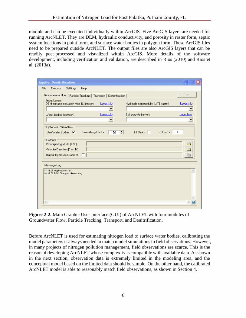
of the model GUI is shown in Figure 2-2; there are four tabs, each of which represents a

separate modeling component. For example, the tab of Groundwater Flow is for estimating

magnitude and direction of groundwater flow velocity, and the tab of Particle Tracking for

estimating flow path from each septic system. Each tab is designed to be a self-contained


6

module and can be executed individually within ArcGIS. Five ArcGIS layers are needed for

running ArcNLET. They are DEM, hydraulic conductivity, and porosity in raster form, septic

system locations in point form, and surface water bodies in polygon form. These ArcGIS files

need to be prepared outside ArcNLET. The output files are also ArcGIS layers that can be

readily post-processed and visualized within ArcGIS. More details of the software

development, including verification and validation, are described in Rios (2010) and Rios et

al. (2013a).

Figure 2-2. Main Graphic User Interface (GUI) of ArcNLET with four modules of

Groundwater Flow, Particle Tracking, Transport, and Denitrification.

Before ArcNLET is used for estimating nitrogen load to surface water bodies, calibrating the

model parameters is always needed to match model simulations to field observations. However,

in many projects of nitrogen pollution management, field observations are scarce. This is the

reason of developing ArcNLET whose complexity is compatible with available data. As shown

in the next section, observation data is extremely limited in the modeling area, and the

conceptual model based on the limited data should be simple. On the other hand, the calibrated

ArcNLET model is able to reasonably match field observations, as shown in Section 4.


7

3. ARCNLET MODELING FOR EAST PALATKA (Lower St. Johns)

3.1. Modeling Area and ArcGIS Input Data

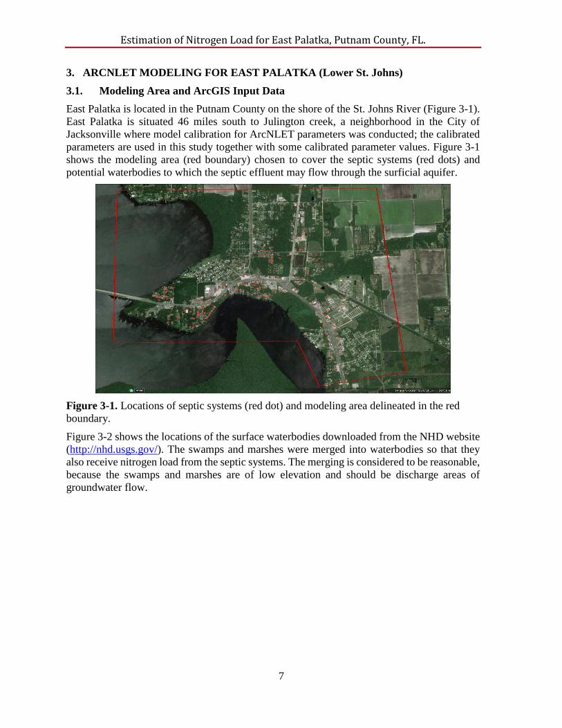
East Palatka is located in the Putnam County on the shore of the St. Johns River (Figure 3-1).

East Palatka is situated 46 miles south to Julington creek, a neighborhood in the City of

Jacksonville where model calibration for ArcNLET parameters was conducted; the calibrated

parameters are used in this study together with some calibrated parameter values. Figure 3-1

shows the modeling area (red boundary) chosen to cover the septic systems (red dots) and

potential waterbodies to which the septic effluent may flow through the surficial aquifer.

Figure 3-1. Locations of septic systems (red dot) and modeling area delineated in the red

boundary.

Figure 3-2 shows the locations of the surface waterbodies downloaded from the NHD website

(http://nhd.usgs.gov/). The swamps and marshes were merged into waterbodies so that they

also receive nitrogen load from the septic systems. The merging is considered to be reasonable,

because the swamps and marshes are of low elevation and should be discharge areas of

groundwater flow.

http://nhd.usgs.gov/


8

Figure 3-2. Locations of waterbodies (red rectangular marked the modeling area)

Figure 3-3 plots the DEM of the modeling area downloaded from the USGS National Map

Viewer and Download Framework (http://nationalmap.gov/viewer.html). The DEM resolution

is 3m × 3m, and it can capture small waterbodies, e.g., the pond, swamp/marsh and small

channel of river marked by the black oval, respectively in Figure 3-3. The pond and

swamp/marsh is also shown in Google Earth (Figure 3-4) but not reflected in the ArcGIS layer

of waterbodies (Figure 3-2). Therefore, the ArcGIS layer of waterbodies was updated manually

to include the missing pond and swamp/marsh as polygons, FIDs are 15, 24 and 25 as shown

in Figure 3-5.

http://nationalmap.gov/viewer.html


9

Figure 3-3. DEM data of the modeling area with the resolution of 3m × 3m. The black oval

delineate the areas where the layer of water body (Figures 3-2) needs to be updated to include

the missing pond/lake, swamp/marsh and part of river.

Figure 3-4. Google Earth image for part of the modeling area. The black oval mark from the

left represents part of river, swamp, and pond/lake consecutively, which reflected in the

DEM (Figure 3-3) but not shown in the layer of surface waterbodies (Figure 3-2).


10

Figure 3-5. Updated waterbodies map based on DEM and Google Earth. The waterbodies

are labeled by their FIDs; the FID of the added small channel of river is 23, ponds are 24 and

15, and the FIDs of the added swamp/marsh is 25.

3.2. Groundwater Flow Parameters

For the groundwater flow modeling, the hydraulic conductivity values are obtained directly

from the Soil Survey Geographic database (SSURGO) database, i.e., the representative values

contained in the database. Since the database does not include porosity data, the data was

evaluated as 1 – (DB/DP), where DB and Dp are bulk density and particle density, respectively;

bulk density was obtained directly from the SSURGO database and particle density was

assumed to be 2.65 gcm-3 that is commonly used in soil physics. The SSURGO database

contains data at the horizon levels; the data were aggregated to the component and

subsequently unit levels, because the hydraulic conductivity and porosity at the soil units are

used in ArcNLET modeling. The aggregation was completed by following the procedure

described in Wang et al. (2011). Figures 3-6 and 3-7 plot the heterogeneous hydraulic

conductivity (spatial distribution in top and contours in bottom figure) and porosity (spatial

distribution in top and contours in bottom figure) fields, respectively, for the soil units in the

modeling area. In Figure 3-6, a mix of low and high values are observed around the St. Johns

River shores, while high values (e.g., 7.95 m/d and 21.6 m/d) of hydraulic conductivity are

shown in most of the domain. Hydraulic conductivity values are assigned to be zero at the river


11

Figure 3-6. Heterogeneous hydraulic conductivity (m/d) (top) and contours (bottom) of soil

units.


12

Figure 3-7. Heterogeneous porosity (top) and contours (bottom) of soil units.


13

by SSURGO. The spatial pattern may be related to the depositional hydrogeology in the

modeling area. A similar pattern was also observed for porosity shown in Figure 3-7. Although

a large number of soil zones are shown in Figure 3-7, the spatial variation is negligible, ranging

between 0.4 and 0.51. Generally speaking, the porosity field can be considered to be

homogeneous in the modeling domain.

The smoothing factor value needed for the flow modeling was taken as 60, which is used in

our previous modeling at the Orange County (Ye and Zhu, 2014) and the Welaka town

(Sayemuzzaman and Ye, 2014). While it is ideal to have head observations for model

calibration so that site-specific value of the smoothing factor can be determined, head

observations at the modeling domain are unavailable.

3.3. Nitrogen Transport Parameters

Table 3-1 lists four sets of values of transport parameters (longitudinal and transverse

dispersivity and denitrification coefficient) used in this study. For the longitudinal and

transverse dispersivities, Davis (2000) used 7 ft. (2.134m) and 0.18 ft. (0.0549m), respectively,

for solute transport modeling in the Naval Air Station located in the City of Jacksonville. In

our previous modeling for the Julington Creek neighborhood (also located in the City of

Jacksonville), the two parameters were calibrated against field observations of nitrogen

concentrations, and the calibrated values are 6m and 2.5m for longitudinal and transverse

dispersivity, respectively. Considering the scaling effect of dispersivity (i.e., dispersivity

increases with spatial scale), the first set of 2.134m and 0.0549m seems more reasonable,

because the modeling area of this study is small. However, due to parametric uncertainty and

given that the two sites are close (within the 60 miles radius) to our modeling area, we adopted

the two sets of parameter values in this study.

The decay coefficient of denitrification is also subject to substantial uncertainty. McCray et al.

(2005) reported a range of 0.004 – 2.27 d-1, and Rios et al. (2013b) used the range of 0.004 –

1.08 d-1 in the recently developed ArcNLET Monte Carlo simulation package. According to

Anderson (1998), denitrification rate is a linear function of particulate organic carbon (POC)

content. Based on the POC comparison between Julington Creek and Welaka town, which is

also located 15 miles apart from East Palatka, 0.011 d-1 was used in Welaka town modeling.

To address uncertainty in the decay coefficient, a low value of 0.001 d-1 was used in Welaka

town modeling. We adopted the same values in this study, i.e., 0.011 d-1 in Cases 1 and 2 and

0.001 d-1 in Cases 3 and 4, to investigate impacts of the coefficient on the load estimation. A

larger load was obtained for the smaller coefficient, as shown in Section 4.

3.4. Nitrogen Load to Groundwater

Nitrogen load from a septic system to groundwater, which is the inflow mass Min (g/d) of

equation 5, is an important parameter in ArcNLET modeling. There are two equivalent ways

of handling the inflow mass: (1) to fix Min and evaluate Z using equation 5 (Z is the source plan

height needed for calculating the mass of denitrification and load), and (2) to fix Z and calculate

Min using equation 5. In this study, the first option was used, and the value of inflow mass was

approximated as nitrogen release per person per day × people/household × 0.7 (the amount of

nitrogen not lost in septic tanks). Instead of using national average, we used the average total

nitrogen (TN) load 11.2 g per person per day (from Marcy Policastro,

[email protected]). The U.S. Census Bureau website

mailto:[email protected]


14

(http://quickfacts.census.gov/qfd/states/12/12095.html) reported that there are 2.53 persons

per household in Putnam County. It is a general consensus that about 30% of nitrogen is

removed in Septic tank (e.g., MACTEC, 2007). Therefore, the input mass from septic to

groundwater is 19.84 g/d (for both commercial and residential), which is smaller than 21.7 g/d

reported in the Wekiva study (Roeder, 2008). Although the commercial loadings are smaller

than the residential, we used the same loadings for the commercial units in the modeling area

to have conservative load estimates. In other words, this value is used for all the individual

septic systems in the modeling sites.

Another quantity needed to use equation (5) for evaluating the inflow mass is the source plane

concentration (C0). It ranges between 0 mg/L and 80 mg/L (McCray et al., 1995), and the

average of 40 mg/L was used in this study.

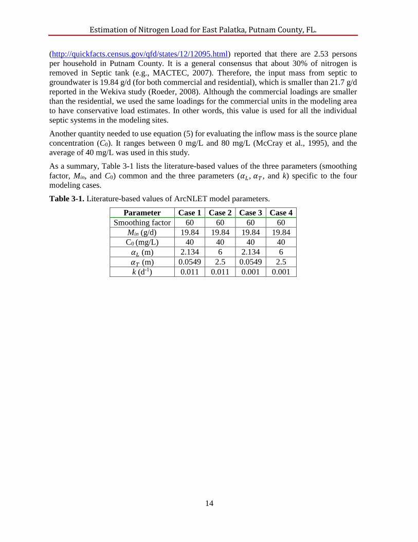
As a summary, Table 3-1 lists the literature-based values of the three parameters (smoothing

factor, Min, and C0) common and the three parameters (𝛼𝐿 , 𝛼𝑇 , and k) specific to the four

modeling cases.

Table 3-1. Literature-based values of ArcNLET model parameters.

Parameter Case 1 Case 2 Case 3 Case 4

Smoothing factor 60 60 60 60

Min (g/d) 19.84 19.84 19.84 19.84

C0 (mg/L) 40 40 40 40

𝛼𝐿 (m) 2.134 6 2.134 6

𝛼𝑇 (m) 0.0549 2.5 0.0549 2.5

k (d-1) 0.011 0.011 0.001 0.001

http://quickfacts.census.gov/qfd/states/12/12095.html


15

4. RESULTS AND DISCUSSION

4.1. Results of Groundwater Flow Modeling

With the data and information described in Section 3, ArcNLET groundwater flow module and

particle tracking module were executed. The flow model provides magnitude and direction of

seepage velocity (Darcy velocity divided by porosity) at the individual raster cells in the

modeling domain. They are used in the particle tracking module to evaluate flow paths from

individual septic systems to receiving waterbodies. Figure 4-1 plots the simulated flow paths.

The St. Johns River (waterbody 23 and 21) has the largest number (158 out of 106) of

contributing septic systems. Waterbody 4 has the second largest number (20) of contributing

septic systems.

Figure 4-1．Simulated flow paths from septic systems to surface waterbodies.

4.2. Nitrogen Transport Modeling Results

Using the nitrogen transport parameter values discussed in Section 3, ArcNLET transport

module was executed. The simulated nitrogen plumes are plotted in Figure 4-2 to Figure 4-5

for the four cases. Table 4-1 to Table 4-4 list the nitrogen load estimates to the receiving

waterbodies and reduction ratios for the four cases with different values of longitudinal


16

dispersivity (αL), horiontal transverse dispersivity (αT), and denitrification coefficient (k) listed

in Table 3-1. Comparing Figure 4-2 of Case 1 with Figure 4-3 of Case 2 shows that, the

simulated plumes become fatter when horizontal transverse dispersivity increases. However,

since the same denitrification coefficient is used for the two cases, the load estimates of the

two cases are similar, as shown in Tables 4-1 and 4-2. When the denitrification coefficient

decreases from 0.011 d-1 in Cases 1 and 2 to 0.001 d-1 in Cases 3 and 4, the load estimates

increase significantly (shown in Figure 4-4 and Figure 4-5 ). Each of the waterbody’s received

loadings can be found in Table 4-3 and Table 4-4 for Case 3 and Case 4, respectively. This is

reasonable because it was found in our previous sensitivity analysis that denitrification

coefficient is the most influential parameter to load estimate (Wang et al., 2012).

For the convenience of comparing the load estimates of the four modeling cases, Table 4-5

lists the total loads (in the units of g/d and lb/yr), load (g/d) per septic system to the surface

water bodies, and the reduction ratios (%) of the four parametric cases. This table shows again

that the load estimates depends more on the denitrification coefficient than on the dispersivities.

For example, Cases 1 and 3 have the same dispersivities (αL = 2.134 m, αT = 0.0549 m) but

different denitrification (0.011 d-1 for Case 1 and 0.001 d-1 for Case 3). The two cases have

dramatically different load estimates, with the estimate of Case 3 being 2.96 times as large as

that of Case 1. The ratio is 2.85 between the estimates of Cases 4 and 2, when the dispersivities

change to another set (αL = 6 m and αT = 2.5 m). The reduction ratio changes from 78% (case

1) and 77% (case 2) to 36% (case 3) and 36% (case 4), when the denitrification coefficient

decreases from 0.011 d-1 to 0.001 d-1. These reduction ratios are comparable with those

reported in literature, as discussed in Ye and Sun (2013).

Figure 4-6 plots the estimated nitrogen loads to the eight waterbodies (with FIDs of 23, 8, 21,

4, 24, 25, 6 and 15) that receive all the nitrogen loads from the septic systems. For all the four

modeling cases, the St. Johns River (FID 23 and FID 21) receives the largest amount of load

with the 67% (106 out of 158) contributing septic systems.


17


for Case 1. Locations of the waterbodies are shown in Figure 4-2.

Waterbody

FID

Load

(g/d)

Load

(lb/yr)

Inflow Mass

(g/d)

Reduction Ratio

(%)

23 491.41 395.50 1745.92 72

8 78.94 63.53 357.12 78

21 44.19 35.56 317.44 86

4 30.46 24.51 396.8 92

24 1.61 1.29 79.36 98

25 0.61 0.49 39.68 98

15 0.25 0.20 39.68 99

6 0.00 0.00 19.84 100

Total 647.47 521.10 3035.52 78

Figure 4-2．Simulated flow paths from septic systems to surface waterbodies. Paramter

values specific to Case 1 are αL = 2.134 m, αT = 0.0549 m, and k = 0.011 d-1.


18



Waterbody

FID

Load

(g/d)

Load

(lb/yr)

Inflow Mass

(g/d)

Reduction Ratio

(%)

23 509.48 410.04 1745.92 71

8 82.48 66.38 357.12 77

21 47.66 38.36 317.44 85

4 32.97 26.53 396.8 92

24 1.95 1.57 79.36 98

25 0.67 0.54 39.68 98

15 0.25 0.20 39.68 99

6 0.00 0.00 19.84 100

Total 675.46 543.62 3035.52 79

Figure 4-3. Simulated flow paths from septic systems to surface waterbodies. Parameter

values specific to Case 2 are αL = 6 m, αT = 2.5 m, and k = 0.011 d-1.


19

Table 4-3. Simulated nitrogen loads to surface waterbodies and groundwater (inflow mass)


Waterbody

FID

Load

(g/d)

Load

(lb/yr)

Inflow Mass

(g/d)

Reduction Ratio

(%)

23 1261.65 1015.41 1785.6 28

4 214.28 172.46 357.12 46

21 184.99 148.88 317.44 42

8 182.68 147.02 396.8 49

24 44.64 35.93 79.36 44

25 16.50 13.28 39.68 58

15 10.00 8.05 19.84 75

6 2.31 1.86 39.68 88

Total 1917.05 1542.89 3035.52 36


values specific to Case 3 are αL = 2.134 m, αT = 0.0549 m, and k = 0.001 d-1.


20



Waterbody

FID

Load

(g/d)

Load

(lb/yr)

Inflow Mass

(g/d)

Reduction Ratio

(%)

23 1265.83 1018.77 1785.6 27

4 215.99 173.83 357.12 46

21 186.43 150.04 317.44 41

8 183.98 148.07 396.8 48

24 45.25 36.42 79.36 43

25 16.81 13.53 39.68 58

15 10.23 8.23 19.84 74

6 2.55 2.05 39.68 87

Total 1927.06 1550.94 3035.52 36


values specific to Case 4 are αL = 6 m, αT = 2.5 m, and k = 0.001 d-1.


21

Table 4-5．Simulated nitrogen loads to surface waterbodies and nitrogen reduction ratios for

the four cases。

Figure 4-6. Nitrogen loading (g/d) to the individual waterbodies for the four modeling cases.

23 8 21 4 24 25 15 6 Total

Case 1 491 79 44 30 2 0.61 0.25 0.00 647

Case 2 509 82 48 33 2 0.67 0.25 0.00 675

Case 3 1262 183 185 214 45 16 10 2 1917

Case 4 1266 184 186 216 45 17 10 3 1927

0

200

400

600

800

1000

1200

1400

1600

1800

Nit

rate

load

(g/d

)

Total load

(g/d)

Total load

(lb/yr)

Load per

septic

systems

(g/d)

Reduction

ratio (%)

Load to

St. Johns

River

(g/d)

Percentage

of total load

to St. Johns

River

Case 1 647 521 4.10 78 536 83

Case 2 675 544 4.28 77 557 82

Case 3 1917 1543 12.13 36 1447 75

Case 4 1927 1551 12.20 36 1452 75


22

CONCLUSION

The ArcNLET modeling of this study leads to the following major conclusions:

1. Data and information needed to establish ArcNLET models for groundwater modeling

and nitrogen load estimation are readily available in the East Palatka. The data are

available in either the public domain (e.g., USGS websites) or FDEP database. Site-

specific data include DEM, waterbodies, septic locations, hydraulic conductivity, and

porosity. The values of smoothing factor, dispersivity, decay coefficient, inflow mass

to groundwater, and source plane concentration are obtained from literature.

2. Among the 158 combined residential and commercial septic systems, 106 septic

systems contribute nitrogen load to the St. Johns River. The rest of septic systems

contribute nitrogen load to waterbodies that are not connected to the St. Johns River.

As a result, not all the removed septic systems contributed to nitrogen load reduction

in the TMDL practice. This suggests importance of considering spatial variability in

environmental management of nitrogen contamination.

3. For all the four modeling cases considered in this study, the load estimate to the St.

Johns River (combined of FID 23 and FID 21) is the largest, with the load ranging from

75% to 83% of the total load.

4. The denitrification coefficient is the most influential parameter to the load estimate.

More effort should be spent to determine the appropriate value of the parameter for

more accurate estimation of load reduction.

Appendix A lists the input and output files of this modeling project. The readers who are

interested in repeating the modeling results may contact Professor Ming Ye ([email protected]) to

request these files.

mailto:[email protected]


23

5. REFERENCES

Anderson, D. (2006), A Review of Nitrogen Loading and Treatment Performance

Recommendations for Onsite Wastewater Treatment Systems (OWTS) in the Wekiva

Study Area, Hazen and Sawyer, P.C.

Blandford, T.N. and T.R. Birdie (1992), Ground-Water Flow and Solute Transport Modeling

Study for Eastern Orange County, Florida and Adjoining Regions, HydroGeoLogic Report

prepared for St. Johns River Water Management District, Orange County Public Utilities

Division, and City of Cocoa, Special Publication SJ93-SP4.

BMAP (2012), Basin Management Action Plan for the Implementation of Total Maximum

Daily Loads for Nutrients and Dissolved Oxygen by the Florida Department of

Environmental Protection in the Santa Fe River Basin, developed by the Florida

Department of Environmental Protection Division of Environmental Assessment and

Restoration Bureau of Watershed Restoration.

Byrme Sr., M.J., R.L. Smith, and D.A. Repert (2012), Potential for Denitrification near

Reclaimed Water Application Sites in Orange County, Florida, 2009, U.S. Geological

Survey Open File Report 2012-1123.

Davis, J. H. 2000. Fate and Transport Modeling of Selected Chlorinated Organic Compounds

at Operable Unit 3, U.S. Naval Air Station, Jacksonville, Florida. U.S. Geological Survey,

Tallahassee FL.Open-file report 00-255.

Domenico, P.A. (1987), An analytical model for multidimensional transport of a decaying

contaminant species. J Hydrol 91:49–58.

Gelhar, L.W., C. Welty, and K.R. Rehfeldt. (1992), A critical review of data on field-scale

dispersion in aquifers. Water Resour. Res. 28: 1955–1974.

Fernandes, R. (2011), Statistical methods for estimating the denitrification rate. Florida State

University, Master Thesis.

Harden, H., J. Chanton, R. Hicks, and E. Wade (2010), Wakulla County Septic Tank Study

Phase II Report on Performance Based Treatment Systems.

Heinen, M (2006) Simplified denitrification models: Overview and properties. Geoderma

133(3-4):444–463

Hicks, R.W. and K. Holland (2012), Nutrient TMDL for Silver Springs, Silver Springs Group,

and Upper Silver River (WBIDs 2772A, 2772C, and 2772E), Ground Water Management

Section, Florida Department of Environmental Protection, Tallahassee, FL.

Horsley, S.W., Santos, D., and Busby, D., 1996, Septic system impacts for the Indian River

Lagoon, Florida, available at

http://water.epa.gov/type/watersheds/archives/upload/2004_05_11_watershed_Proceed_s

ess41-60.pdf, accessible as of 1/20/2014.

MACTEC, (2007). Phase I Report Wekiva River Basin Nitrate Sourcing Study. Newberry, FL:

MACTEC http://www.dep.state.fl.us/water/wekiva/docs/phase-i-final-report.pdf

http://water.epa.gov/type/watersheds/archives/upload/2004_05_11_watershed_Proceed_sess41-60.pdf

http://water.epa.gov/type/watersheds/archives/upload/2004_05_11_watershed_Proceed_sess41-60.pdf


24

MACTEC, Inc. 2007. Phase I Report: Wekiva River Basin Nitrate Sourcing Study. Prepared

for St. Johns River Water Management District and Florida Department of Environmental

Protection.

Maggi, F., C. Gu, W.J. Riley, G.M. Hornberger, R.T. Venterea, T. Xu, N. Spycher, C. Steefel,

N.L. Miller, C.M. Oldenburg (2008), A mechanistic treatment of the dominant soil nitrogen

cycling processes: Model development, testing, and application. J Geophys Res.

doi:10.1029/2007JG000578.

McCray, J.E., M. Geza, K.F. Murray, E.P Poeter, D. Morgan (2009), Modeling onsite

wastewater systems at the watershed scale: a user’s guide. Water Environment Research

Foundation, Alexandria, VA.

McCray, JE, Kirkland SL, Siegrist RL, Thyne GD (2005) Model parameters for simulating

fate and transport of on-site wastewater nutrients. Ground Water 43(4):628–639.

O'Reilly, A.M., N.-B. Chang, and M. P. Wanielista (2012a), Cyclic biogeochemical processes

and nitrogen fate beneath a subtropical stormwater infiltration basin, Journal of

Contaminant Hydrology, 133, 53–75.

O'Reilly, A.M., M.P. Wanielista, N.-B. Chang, Z. Xuan, W.G. Harris (2012b), Nutrient

removal using biosorption activated media: Preliminary biogeochemical assessment of an

innovative stormwater infiltration basin, Science of the Total Environment, 432, 227–242.

Otis, R.J., Anderson, D.L., and Apfel, R.A., 1993, Onsite sewage disposal system research in

Florida: Report prepared for Florida Department of Health and Rehabilitative Services,

Contract No. LP-596, Ayres and Associates, Tampa, Fla., 57 p.

Phelps, G.G. (2004), Chemistry of Ground Water in the Silver Spring Basin, Florida, with an

Emphasis on Nitrate, U.S. Geological Survey, Reston, Virginia, Scientific Investigations

Report 2004-5144

Reddy, K.R., P.D. Sacco, and D.A. Graetz (1980), Nitrate reduction in an organic soil-water

system, Journal of Environmental Quality, 9(2), 283-288.

Rios, J.F. (2010), A GIS-Based Model for Estimating Nitrate Fate and Transport from Septic

Systems in Surfacial Aquifers, Master Thesis, Florida State University, Tallahassee, FL.

Rios, J.F., M. Ye, and L. Wang (2011a), uWATER-PA: Ubiquitous WebGIS Analysis Toolkit

for Extensive Resources - Pumping Assessment, Ground Water, 49(6), 776-780, DOI:

10.1111/j.1745-6584.2011.00872.x.

Rios, J.F., M. Ye, L. Wang, and P. Lee (2011b), ArcNLET: An ArcGIS-Based Nitrate Load

Estimation Toolkit, User’s Manual, Florida State University, Tallahassee, FL., available

online at http://people.sc.fsu.edu/~mye/ArcNLET/users_manual.pdf.

Rios, J.F., M. Ye, L. Wang, P.Z. Lee, H. Davis, and R.W. Hicks (2013a), ArcNLET: A GIS-

based software to simulate groundwater nitrate load from septic systems to surface water

bodies, Computers and Geosciences, 52, 108-116, 10.1016/j.cageo.2012.10.003.

Rios, J.F., M. Ye, and H. Sun (2013b), ArcNLET 2.0: New ArcNLET Function of Monte Carlo

Simulation for Uncertainty Quantification, Florida State University, Tallahassee, FL.


25

Roeder, E. (2008), Revised Estimates of Nitrogen Inputs and Nitrogen Loads in the Wekiva

Study Area. Available online at http://www.dep.state.fl.us/water/wekiva/docs/dohwekiva-

estimate-final2008.pdf.

Sayemuzzaman, M. and Ye M. (2014), Estimation of Nitrogen Load from Septic Systems to

Surface Waterbodies in Welaka Town, Putnam County, FL, technical report prepared for

FDEP, unpublished.

Srinivasan V, Clement TP, Lee KK (2007) Domenico solution – is it valid? Ground Water

45(2):136–146.

Sumner, D.M. and L.A. Bradner (1996), Hydraulic Characteristics and Nutrient Transport and

Transformation Beneath a Rapid Infiltration Basin, Reedy Creek Improvement District,

Orange County, Florida, U.S. Geological Survey, Water-Resources Investigations Report,

95-4281.

Ursin, E.L. and E. Roeder (2008), An assessment of nitrogen contribution from onsite

wastewater treatment systems (OWTS) in the Wekiva study area of central Florida. In

National Onsite Wastewater Recycling Association (NOWRA) Nitrogen Symposium.

Florida Department of Health, Tallahassee.

U.S. EPA (2003), Voluntary National Guidelines for Management of Onsite and Clustered

(Decentralized) Wastewater Treatment Systems. U.S. Environmental Protection Agency.

U.S. EPA. (2010), Water Quality Standards for the State of Florida’s Lakes and Flowing

Waters; Proposed Rule. Released by EPA on January 14, 2010.

http://edocket.access.gpo.gov/2010/pdf/2010-1220.pdf.

U.S. EPA (2013), A Model Program for Onsite Management in the Chesapeake Bay Watershed,

Office of Wastewater Management, U.S. Environmental Protection Agency.

Valiela, I. and J.E. Costa (1988), Eutrophication of Buttermilk Bay, a Cape Cod coastal

embayment: Concentrations of nutrients and watershed nutrient budgets. Environmental

Management 12, no. 4: 539–553.

Valiela, I., G. Collins, J. Kremer, K. Lajtha, M. Geist, B. Seely, J. Brawley, C.H. Sham (1997)

Nitrogen loading from coastal watersheds to receiving estuaries: new method and

application, Ecological Applications, 7(2), 358–380.

Valiela, I., M. Geist, J. McClelland, and G. Tomasky (2000), Nitrogen loading from

watersheds to estuaries: Verification of the Waquoit Bay Nitrogen Loading Model.

Biogeochemistry 49, no. 3: 277–293.

Wang, L., M. Ye, J.F. Rios, and P. Lee (2011), ArcNLET: An ArcGIS-Based Nitrate Load

Estimation Toolkit, Application Manual, Florida State University, Tallahassee, FL.,

available online at http://people.sc.fsu.edu/~mye/ArcNLET/application_manual.pdf.

Wang L, Ye M, J.F. Rios, Lee P (2012). Sensitivity analysis and uncertainty assessment for

ArcNLET-estimated nitrate load from septic systems to surface water bodies.

http://people.sc.fsu.edu/~mye/ArcNLET/ArcNLETSensitivityUncertainty.pdf

Wang, L., M. Ye, J.F. Rios, R. Fernandes, P.Z. Lee, and R.W. Hicks (2013), Estimation of

nitrate load from septic systems to surface water bodies using an ArcGIS-based software,

Environmental Earth Sciences, doi:10.1007/s12665-013-2283-5.

http://edocket.access.gpo.gov/2010/pdf/2010-1220.pdf

http://people.sc.fsu.edu/~mye/ArcNLET/ArcNLETSensitivityUncertainty.pdf


26

Wanielista, M., N.-B. Chang, Z. Xuan, L. Naujock, and P. Biscardi (2011), Nitrogen Transport

and Transformation Beneath Stormwater Retention Basins in Karst Areas and

Effectiveness of Stormwater Best Management Practices for Reducing Nitrate Leaching to

Ground Water Marion County, Florida, Florida Department of Environmental Protection,

FDEP Report # S0316.

West, MR, Kueper, BH, Ungs, MJ (2007) On the use and error of approximation in the

Domenico (1987) solution. Ground Water 45(2): 126–135.

Ye, M, Sun H (2013), Estimation of Nitrogen Load from Removed Septic Systems to Surface

Water Bodies in the City of Port St. Lucie, the City of Stuart, and Martin County, Technical

report submitted to Florida Department of Environmental Protection, Florida State

University, Tallahassee, FL., available online at

http://people.scs.fsu.edu/~mingye/FDEP/PortStLucieModeling.pdf, accessed as of

8/12/2014.

Ye, M and Y. Zhan (2014), Estimation of Groundwater Seepage and Nitrogen Load from

Septic Systems to Lakes Marshall, Roberts, Weir, and Denham, technical report prepared

for FDEP, unpublished.

http://people.scs.fsu.edu/~mingye/FDEP/PortStLucieModeling.pdf


27

APPENDIX A

The following files were used in the ArcNLET modeling. The readers who may repeat the

ArcNLET modeling using the input files listed below, and their modeling results should be the

same as the output files listed below. Bracket represents the name of the files saved for re-run.

List of Input Files:

1. DEM_NED-3m×3m (dem_ned)

2. Waterbody-NHD-River, Lakes, Ponds, Swamps and Marshes (nhd_merge.shp)

3. Septic tank location file (Palatka_Sewer_Points_10102014_Prj.shp)

4. Heterogeneous Porosity (porosity)

5. Heterogeneous hydraulic conductivity (hydcond)

List of Output Files:

1. Smoothed DEM of the first round of smoothing with the smoothing factor of 60 and

then mosaic the waterbody: (demS60_afMosaic.img).

2. DEM file for the waterbodies: (wb_extract)

3. Smoothed DEM after including the waterbodies elevation and having of the second

round of smoothing with the smoothing factor of 5: (demS60_5.img)

4. Seepage velocity final: velocity magnitude (vel_magS60_5.img) and velocity direction

(vel_dirS60_5.img)

5. Simulated flow path: Particle paths (partPath_S60_5)

6. Simulated plume for Case 1: Geodatabase files for Info and raster files for plume

distribution (plume_case1_info)






distribution (plume_case4_1_info)

Date post:	07-Aug-2015
Category:	Documents
Upload:	mohammad-sayemuzzaman-phd-fe
View:	66 times
Download:	0 times

East Palatka_Nitrogen Modeling_Report

Documents