Econ 831 Notes - Simon Fraser University

Econ 831 Math Econ Sept 13, 2010

Page 1 of 61

Sample Space Problem of the Day: A family has two kids, one of them is a girl. What is the probability that both kids are girls?

To solve the problem, we need to have a statistical model.

Statistical model is a set of assumptions A1: For each kid, Pr Pr 0.5 A2: The gender of the two kids are independent

Sample Space is the list of elementary events with their probability of occurrence.

Interpretation of the Problem

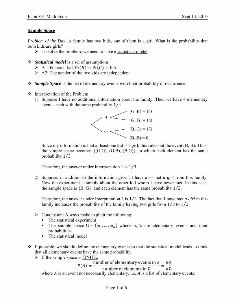
1) Suppose I have no additional information about the family. Then we have 4 elementary events, each with the same probability 1 4⁄ .

Since my information is that at least one kid is a girl, this rules out the event (B, B). Thus, the sample space becomes (G,G), (G,B), (B,G), in which each element has the same probability 1 3⁄ . Therefore, the answer under Interpretation 1 is 1 3⁄ .

2) Suppose, in addition to the information given, I have also met a girl from this family. Now the experiment is simply about the other kid whom I have never met. In this case, the sample space is B, G, and each element has the same probability 1 2⁄ . Therefore, the answer under Interpretation 2 is 1 2⁄ . The fact that I have met a girl in this family increases the probability of the family having two girls from 1 3⁄ to 1 2⁄ .

Conclusion: Always make explicit the following: The statistical experiment The sample space Ω , … , where ’s are elementary events and their

probabilities The statistical model

If possible, we should define the elementary events so that the statistical model leads to think

that all elementary events have the same probability. If the sample space is FINITE,

number of elementary events in number of elements in Ω

##Ω

where is an event not necessarily elementary, i.e. is a list of elementary events.

B

G

(G, B) = 1/3

(G, G) = 1/3

(B, G) = 1/3

(B, B) = 0


Page 2 of 61

In this case, is the uniform probability on Ω, Ω 0, 1

##Ω


Page 3 of 61

Algebras and -Algebras of Events Problem: I throw a piece of chalk on the blackboard. What is the probability for the chalk to hit below the given curve?

Sample space: Ω Statistical model

Assume that all the points on the blackboard have the same probability of being hit. Then, Ω 0. That is, if we ask about the probability of a single point being hit, the answer is going to be zero. Therefore, we need to resort to a different measure of probability—expressed as the area under a curve.

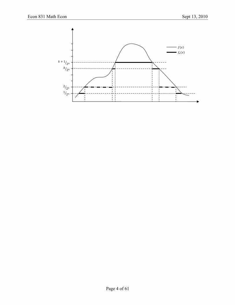
In the cases of constant and step-functions, the probability of the chalk hitting inside is

Ω. We can extend this idea to any function .

To find the probability of an event in general, given a function . • Define the event as

, Ω • Define the events as

, Ω where

2 ,

1 21

20

♦ for all and all ♦ lim

1 3⁄ A step-function


Page 4 of 61

12

22

2

12


Page 5 of 61

Algebras and -Algebras (Cont’d)

Recap. Let , Ω Let , Ω and ∑

We can show 1) , 2) is increasing implies that has a limit. Thus, lim for all . As a result of (1) and (2), , is such that , i.e. is increasing. Therefore, , and we can say

lim We can define for any set , such that

lim lim

More generally, whenever, is Riemann integrable, we can get by using the step-wise approximation.

Conclusion: For any sample Ω, the events for which I can define are the subsets of Ω including at least Ω itself (by definition, Ω 1) If exists, then 1 If and are included, then is included, and also If is included in , and all the ’s are such that exist, then has

to be included.

Definition. Let Ω be the sample space. An algebra of events of events of Ω is a family of subsets of Ω (i.e. Ω ) such that

1) Ω 2) 3) ,

is a -algebra (or -field) if in addition, we have 4) ,

Remark. If is an algebra, , … , finite collection of sets such that , 1, … , , then , and

Note. By the De Morgan’s Law, . Remark. If Ω is finite and Ω , then algebra -algebra

Note. If Ω is infinite, then -algebra algebra (but not reverse, see e.g. on P.11)

Theorem. If Ω is countable and is a -algebra of Ω such that , then Ω

Proof. We will demonstrate the equality by showing Ω and Ω . First, by the definition of a -algebra, Ω .


Page 6 of 61

Next, to show that Ω , we need to show that Ω . Since Ω is countable, we can describe its elements as

Ω , … , , … Consider the following sets defined for as , … , . It is easy to show that and (e.g. by recurrence: ). Now consider any set Ω , we can always rewrite as

Ω

lim

lim lim


Page 7 of 61

Probability Measure

Definition. Let Ω, be a measurable space, where Ω is the sample space and is a -algebra.

is a measure on Ω, if and only if

is such that

1) 0 2) ∑

where are pair-wise disjoint sets with for all . is a probability measure if and only if

is a measure Ω 1

Therefore, 0, 1

Remark. If , , then .

Consider countable collection , , , … , , use (2) and (1) Remark. If , , then Remark. Consider the measure space Ω, , , and 0 ∞ . The

associated probability measure on , is defined as

Note. ( ?)

Uniform Probability Measure Ω is finite:

1#Ω , Ω

Ω is infinite (and not countable), e.g. Ω . I can define the Lebesgue Measure on , which is

,

Consider Ω (think of as the blackboard), with 0 ∞. From the Lebesgue measure (area of ) on , I can define uniform probability measure on as

,

Empirical Probability Measure

Assume we have a statistical experiment with draws Ω. After repetitions of the experiment, we have , … , . The sampling frequency of

is given by


Page 8 of 61

1

E.g. could be “rolling a dice and get 3” or “rolling a dice and get 3, 4, 5” We can show that is a probability measure.

Law of Large Numbers (LLN)

Remark. We want to understand the connection between and , where the latter is the population (“genuine”) probability of event .

E.g. Toss a coin

If I repeat my experiment times

#

Sample space: Ω ,

under the assumption that 1) Tosses are independent 2) 1 2⁄

12 , Ω

• Strictly speaking, it is possible to only get heads with probability 1 2⁄ . In this case, 1, which does not converge to 1 2⁄ . However,

11

2 0 Here, we need to understand the meaning of converges to with probability approaching 1.

Definition. Monotone sequence A sequence is called an increasing sequence with limit:

lim lim

A sequence is decreasing with limit:

lim lim

A monotone class is a class that contains the limits of all its increasing and decreasing sequences. A -algebra is a monotone class (this is true by the last theorem in homework 1).

Head

Tail 1Head

Tail

Tail

Head


Page 9 of 61

A class is a collection of sets.

Theorem. Monotone Continuity of Probability Measure Consider a probability measure on Ω, where is a -algebra Suppose is an increasing (and countable) sequence in , and a

decreasing (countable) sequence in . Then, 1) lim lim 2) lim lim


Page 10 of 61

Monotone Continuity Theorem (cont’d)

Theorem. Monotone Continuity of Probability Measure. Consider a probability measure on Ω, where is a -algebra Suppose is an increasing (and countable) sequence in , and a

decreasing (countable) sequence in . Then, 1) lim lim 2) lim lim

Proof. We can define a sequence of disjoint sets such that \ ,

Note. . (We can justify this claim by induction.)

lim

\

\

lim \

lim \

lim

Definition. Limit Superior and Limit Inferior:

lim sup

occurs infinitely many times.

lim inf

occurs eventually. Ω, a -algebra, , Ω. What does it mean to say lim sup ??

lim sup ,

Similarly, lim inf ,

Reference: http://en.wikipedia.org/wiki/Limit_superior_and_limit_inferior#Special_case:_discrete_metric


Page 11 of 61

is an event because it is in the sample space Ω with Ω ,

is the set containing all the ’s that converge to , i.e. 1 2⁄ .

0, ,

, ,1

1

Note. Union corresponds to existential quantifier, and intersection to universal quantifier: , and, .

lim lim | |1

lim lim sup| |1

Recall: 1

with , , getting H Ω

Definition. Almost Surely Convergence and Probability Convergence

. . 0 sup 0

0 | | 0


Page 12 of 61

Convergence

Recall the two definitions Convergence in probability

0 | | 0 0 | | 1

Convergence almost sure . .

0 sup 0

0 sup 1

Note. . .

In general, however, the reverse does not hold. Consider

sup

Convergence almost sure is the Strong LLN • This is the stochastic analog of “pointwise convergence”.

Convergence in probability is the Weak LLN • Continuous Mapping Theorem. For every continuous function , if , then

.


Page 13 of 61

Quality Control and Sampling with / without Replacement

Sampling with / without Replacement Population of individuals Draw individuals among

1st experiment (with replacement):

Draw 1 individual from the population (this is #1). Put it back Draw 1 individual from the population (this is #2). Put it back …

Sample space

Ω , … , where #Ω Assuming independent draws, then

1

2nd experiment (without replacement):

Draw 1 individual from the population This is #1

Draw 1 individual from the remaining population This is #2

…

Sample space: Ω , … ,

where Ω Ω with #Ω 1 2

The two experiments / models are compatible.

defined on Ω defined on Ω , Ω We can move from the 1st experiment to the 2nd experiment by precluding repetition

Probability of having no repetition probability of Ω within Ω, Ω , #Ω#Ω

In both experiments, order matters.

Intuition 1. When is sufficiently smaller than .

Then the probability of no repetition is really large almost 1 1 … 1

Application: for survey polls, is usually quite large compared to ; so we can do calculations with repetitions.


Page 14 of 61

Intuition 2. When is sufficiently close to (extreme case: )

1 2 3 4 5 6 7

Probability of no

repetition ( ⁄ )

1 0.5 0.222 0.094 0.038 0.015

0.006 (99.4%

chance of having a

repetition!) Note. ! • The number of ways to choose an ordered sequence (without repetition) of all

individuals. = number of permutations of the set of individuals

• More generally !

!

♦ is the number of ordered (or arranged) samples of size without

repetitions in a population of size . ♦ Of course, several of these ordered samples share the exact same individuals

but ordered in a different way (there are ! ways of permuting individuals) ♦ The number of subsets of individual in a population of size without

repetition is given by the Binomial coefficient:

!!

! !

♦ Permutation (order matters) !

!

♦ Combination (order does not matter) !

! !

Quality Control without Replacement in Sampling light bulbs with deficient ones

Note. is not random. Minimum quality standard: No more than among are allowed to be deficient.

But it’s too expensive to check the light bulbs. So select randomly light bulbs among , observe deficient ones.

Question: Given , , , , what values are likely for ? (want to be smaller than ) We want to assess: observed and realize it depends on (if is large, then the

probability of observing a large is high, and vice versa). Conversely: we have observed . It makes more likely the value of for which

observed large • Given ,

♦ Note. Probability function indexed by .


Page 15 of 61

• Given , ♦ Note. This is the likelihood function.

Sample Space

1st choice: Ω 0,1,2, … , • However, this sample space is not convenient! Because the probabilities of the

elementary events are not equal, i.e. probability distribution is not uniform.

2nd choice: Ω the ordered samples that can be drawn without replacement. • For this sample space, we can define a uniform probability distribution.

deficient bulbselementary event

##Ω

probability of getting deficient bulbsfrom a sample of size in an ordered way

number of ways to orderthe defective bulbs

3rd choice: Ω the subsets • Uniform probability is induced from uniform probability with ordered samples.

deficient bulbs##Ω

• This is the most appropriate sample space for the question.

Remark. We end up with a probability that is not uniform on 1,2, … ,

,

This characterizes any event Ω This is the hypergeometric distribution, , ,

Econ 831 Math Econ Oct 4, 2010

Page 16 of 61

Quality Control (cont’d)

Recap Population: Defective light bulbs: Quality control:

Sample with defect

Case 1. Draw without replacement Ω arranged samples

Ω

Each sample in Ω corresponds to exactly ! arranged sample in Ω. means the probability of getting defective bulbs in a set of bulbs.

Case 2. Draw with replacement

Ω samples that are arranged.

1

1 • ⁄ is the population probability of picking a defective light bulb.

I have defined the Binomial probability distribution , . Remark. If I consider Ω sample where the arrangement does not matter (with

replacement). There is no way we can define a uniform probability from Ω to Ω . • E.g. 2, and , , … ,

Ω Ω, ,, ,, ,

1 gives the probability of success (picking a defective

bulb) in one draw. • 1 is the probability of picking a sequence with sucessses, exactly. • There are such sequences


Page 17 of 61

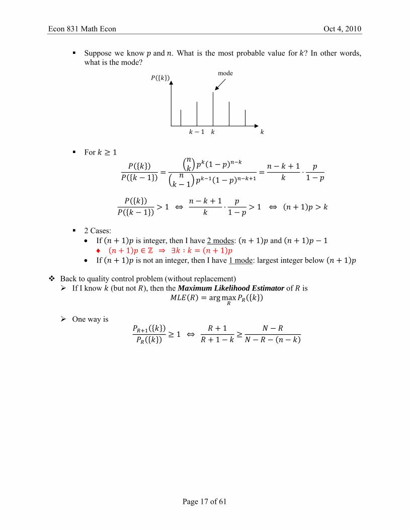
Suppose we know and . What is the most probable value for ? In other words, what is the mode?

For 1

11

1 1

11

1 1 1

1 1 1

2 Cases: • If 1 is integer, then I have 2 modes: 1 and 1 1

♦ 1 1 • If 1 is not an integer, then I have 1 mode: largest integer below 1

Back to quality control problem (without replacement)

If I know (but not ), then the Maximum Likelihood Estimator of is arg max

One way is

1 1

1

mode

1


Page 18 of 61

Quality Control (cont’d)

We are not interested in estimating , but testing whether # deficient ones quality standard

Defining a test is equivalent to defining a critical region that tells me when I should reject

This is true because we assume that

Critical region:

is the “rejection zone,” because we want . is the critical value.

Have to pick “much larger” than ; that is,

2 situations and 2 errors associated with the decision I take after running the experiment: Result

Truth Reject Not Reject

true Type I Error

true Type II Error

Neyman’s approach:

min , subject to

Pick (e.g. 1% or 5%) is the probability of making Type I Error.

For each , find Define Given (result of your experiment), decide whether or not to reject

Quality Control when Sampling with Replacement

, where ⁄ is the true probability of having deficient bulbs of :

arg max 1likelihood function of

It is often useful to take the log-transformation of the likelihood function: arg max arg max ln 1

Then, we can differentiate w.r.t. , set FOC equal zero, and solve for .


Page 19 of 61

Define critical region:

critical value associated with

Extension: Multinomial distribution

We have different colors, call them , … , , each with probability of being picked. Draw a sample of with replacement and independence

Ω , … , , , … , • Here we care about the order of ’s

, … , with

The probability of observing (un-ordered)

with ∑ . is the number of configurations: • Choose pick spots among the available

• Choose pick spots among the left

• Then,

!∏ !

Result: For , … , such that 0,1 and ∑ 1, The multinomial distribution ; , … , :

!∏ !

if with 0,

0 otherwise

This is a probability distribution on 0,1, … ,

Multinomial when 2, ; , and 1 . The distribution is about , 0,1, … , Ω

The binomial , is a distribution about 0,1, … , Ω


Page 20 of 61


Page 21 of 61

Counting Process

Events that occur over time (e.g. event could be a customer entering a store) A counting process is a stochastic process 0 such that

It is non-negative, i.e. 0 is an integer Non-decreasing, i.e.

Independence of 2 events occurring in 2 different (disjoint) time intervals Poisson Process. For an interval of size 0,

1 event

Here is the intensity of arrival. more than 1 event

0 In the same sense, we are interested in events that do not happen too often.

Question: What is the probability of observing events in the time interval 0, ?

We divide 0, into sub-intervals of length Δ ⁄ . Consider intervals 0, Δ , Δ , 2Δ , …, and treat them as consecutive experiments For each interval,

observe exactly 1 event observe more than 1 event

1 observe 0 event I have

⁄

and

⁄ 0 0

Recall the multinomial formula:

interval with exactly 1 event interval with more than 1 event

interval with 0 event!

! ! ! 1

What happens when ∞ while , remains fixed / finite?

!! 1 2 1


Page 22 of 61

!! ! ! 1

1

! !very small unless

this is of order

1

1 exp log 1

For small , log 1 . So the probability is constant as ∞. Then,

interval with 1 event exactly interval with 0 event

1! 1

1!

This approximately works for finite and large enough. Therefore, we have defined the Poisson distribution with parameter over 0 :

events1!

Check that ∑ events 1. this is true from the fact that the summation is a Taylor expansion for .

The only important parameter of the Poisson distribution is .


Page 23 of 61

Real Random Variable

The Lebesgue Measure Example: I draw randomly a number between 0 and 1. What is the probability that

0.47 ? Choice for the first decimal number:

0,1,2,3 0, … ,9 4 0, … ,6

Then, a total of 47 choices out of 100, namely

0.4747

100 0.47 In the book, they calculate 0.47 proof 0.47 0.

Define an infinite sequence of decimal digits and element must coincide with the decimal digits of

0.47 lim lim1

10 0

Definition. The Borel sets of are the smallest -algebra of containing all the open intervals in .

Any interval is a Borel set (but not every Borel set is an interval), and the set of all Borel sets is a -algebra.

(all possible) Borel sets = Borel ring = Borel field = Borel -algebra Theorem.

∞ ,

the smallest ‐algebra containingall the semi‐open intervals ,

Intervals → algebra spanned by intervals

,

Definition. Outer Measure. Suppose

is an algebra on Ω is -additive (i.e. countably additive) on with Ω 1

Then, the outer measure of any Ω is

inf such that

For any set , we can show that .

First, we show Since , we can define and for all 2. Then,


Page 24 of 61

Therefore, is actually the inf over all possible sequences. inf

Second, we show that . We know (by assumption) that . Define

Clearly, is increasing, and is also increasing to .


Page 25 of 61

Recap

is an algebra on Ω is -additive on with Ω 1 Outer measure of Ω

inf such that

We have shown that

Continue to prove that For any such that , define

Note that is an increasing sequence, and is increasing towards . We then have

lim∑

At the limit,

This inequality is true for any sequence with . Therefore, we can conclude that the inequality remains over the infimum

inf such that

Theorem (admitted). is the unique probability measure on Ω, such that

Remark. is defined for any Ω, but we cannot say that is a probability measure on Ω, Ω . This can be proved for the uniform probability measure on ,

The Lebesgue measure on , is defined such that

lim 2 , where is the uniform probability measure on ,

,length of ,

length of ,length of ,

2

is a positive measure on , with convention ∞ ∞,

Warning: only if ∞


Page 26 of 61

Similarly, lim lim only if ∞ for any . Counter-example: , ∞ where

lim 2 , ∞ However, lim . This is not equal to lim 0. The disagreement results from the fact that we cannot find an such that ∞ for .

Multivariate extension

∞,

is the smallest -field containing all ∏ ,

Lebesgue measure on , lim 2 , ,


Page 27 of 61

Random Variable and Random Vectors (r.v.)

(informally) A random variable is a function of the outcome of a statistical experiment. Example.

Ω = sample space of sequences of Bernoulli trials , … , with 0,1 . Ω is endowed with a probability measure:

Ω ∑ 1 ∑ So the probability space is Ω, Ω , . • We don’t need the binomial coefficient here because we’re only considering one

observation. The random variable is defined as

Ω 0,1, … ,

The associated probability is 1

where Ω with Ω (i.e. Ω ). • The probability measure induces another probability measure on 0,1, … ,

defined by

Ω

Ω

• Remark. We say that , . is the probability distribution (or law) of r.v.

More general case. Consider a probability space Ω, , . Define

Ω with Ω is not only countable part of Ω is the range (i.e. the minimum codomain). If Ω is countable, then the range of

should also be countable. should not be sufficient to characterize • This is true because singletons have probability zero if is in a continuum. • Example. Suppose , . Then, 0. So we cannot characterize .

Hopefully, we can use intervals.

∞,

1 if

if

0 if

,

We need to know that ∞, makes sense, because

∞, ∞,


Page 28 of 61

That is, I need to know that ∞, for all .

Definition. Ω, measurable space Ω is -measurable if

∞, Ω is -measurable if

∞,

The pre-image of Borel sets should belong to the -algebra. Definition. If Ω, , is a probability space, any function Ω which is -

measurable is called random variable.

Theorem. Suppose Ω , Ω

is -measurable if and only if . Proof. If is true. Then, it must be true, in particular, that

∞, .

Then, by definition is -measurable. Suppose is -measurable. That is,

∞, .

Need to show that .

Recall that ∏ ∞, . We have to show that

Or we need to show that .

Comments. We know that .

But what is not clear is that .

Note that the converse is clear, since

because

‐field

Lemma 1. Suppose Ω Ω

with being a -field on Ω . Then, is a -field on Ω.


Page 29 of 61

Lemma 2.

. From the above discussion and Lemma 1, we have

It remains to be proved that

. Define

. It can be shown (verify!) that is a -field.

.

Conclusion. When we have a function Ω with underlying probability space

Ω, , , then we say that is -measurable if and only if .

The smallest -field that makes measurable is equal to the pre-image of the Borel -field.

Note. is the smallest -field that makes measurable. Then, the probability distribution of is a probability measure on , :

Hence, is induced by .

When we say that ,

we mean

, for any , , . But we don’t really care about the original Ω, , .


Page 30 of 61

Distribution Function

For any r.v. Ω,

Probability distribution of is , which is a probability measure on , , defined by

and characterized by ∞, ∞, .

We can use a cumulative distribution function to characterize 0,1

Remark. Can we characterize ?

1) must be non-decreasing 2) 0 and 1 3) is right-continuous

lim1

• Why might not be left-continuous?

lim1

Thus, is left-continuous at if and only if 0.

1


Page 31 of 61

Cumulative Distribution Function

0,1 such that is Non-decreasing 0 and 1 Right-continuous

Question: Is it sufficient to define in order to characterize ?

Yes! From I can define a -additive function on all the intervals

, , , ∞ 1

Then, we can construct the outer measure

Unique Coincides with on the set of the intervals

is a probability measure on ,

Density Function

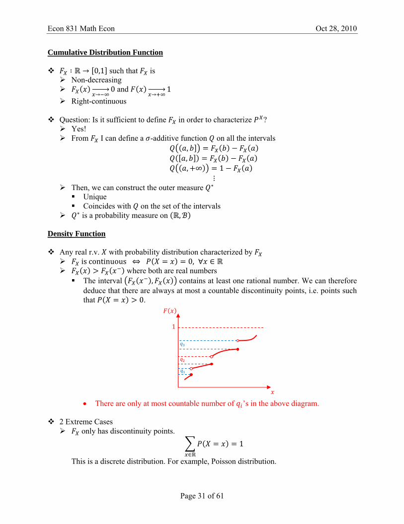
Any real r.v. with probability distribution characterized by is continuous 0, where both are real numbers

The interval , contains at least one rational number. We can therefore deduce that there are always at most a countable discontinuity points, i.e. points such that 0.

• There are only at most countable number of ’s in the above diagram.

2 Extreme Cases only has discontinuity points.

1

This is a discrete distribution. For example, Poisson distribution.

1


Page 32 of 61

is continuous. If is differentiable on with continuous derivative , then we need 0. In addition,

.

When ∞,

1.

(General Case) Definition. is absolutely continuous if and only if 0

Remark. may not be everywhere differentiable. Remark. is not unique, (it is defined up to a set of measure zero). Absolutely continuous functions are those that can be differentiable almost everywhere.

Example. Exponential Distribution.

1 ⁄ 1 ⁄ 00 0

is continuous is not differentiable at 0

lim lim1 ⁄ 1 1

lim1 ⁄ 1

However, the derivative on the left is equal to zero.

Econ 831 Math Econ Nov 1, 2010

Page 33 of 61

Absolute Continuity

Definition. is absolutely continuous if and only if

0 .

Interpretation: When is absolutely continuous, its probability distribution can be

characterized in 2 ways: The CDF (with its 3 properties) The PDF with

0 1, where is almost unique (cf Lebesgue measure zero)

Connection between and :

∆ , ∆∆

lim∆

∆∆

Also, for ∆ small enough, we can use the following approximation: ∆ ∆

Gamma Distribution, Γ , , , 0.

1Γ

⁄

Question: Is a PDF? 1Γ

⁄ 1Γ

⁄

I want Γ to be such that

Γ1 ⁄

Change of variable: ⁄ , so that 1⁄

Γ

This is the Gamma function. There is no closed (or explicit) form for Γ . It is only defined through the integral. The Gamma function is a continuous analog of factorials.

Properties of the Gamma Function

If 1, then Γ 1 Γ 1 If , then Γ 1 !

Proof. Use integration by parts:

Γ

Define


Page 34 of 61

1

Apply integration by parts:

Γ 1

Γ , , then Γ , 1 Γ

Proof. ⁄

Γ Γ ,

where ⁄ .

Multivariate Extension:

, , , ,

where

, , , , 1, ,

1, , , ,

1

For small enough and : , ,


Page 35 of 61

Lebesgue Integral and Mathematical Expectation

1st case: is discrete r.v. is finite or countable, and 1.

is like the Ω in previous lectures. Assume we repeat times the statistical experiment and we get: , , … ,

’s represent the th experiment and they all follow the same distribution (iid) For all , the sampling distribution is

# of times that value occurs# of experiments relative frequency of

where is the number of times I observe the value . Then, we can derive the mathematical (or population) expectation of

1 1if applies

Here we use instead of because we’re talking about the realizations, not the random variables. We could have used instead, in which case we’ll be referring to the random variable before the experiments.

Example 1. We draw (with replacement) balls from a box that contains a proportion of

green balls. : number of green balls picked during experiment # Here , . Then,

,1

1 !! ! 1

1 !! 1 ! 1

Here 1

Example 2.

! 1 ! !

CDF of Poisson distribution:

; , !

2nd case : absolutely continuous , ∆ ∆


Page 36 of 61

, ∆ ∆

well‐defined if | |

Example. Γ ,

1Γ

⁄ 1Γ 1

⁄

,

This leads to the linearity of the expectation operation :

This property is not limited to the Gamma distribution.


Page 37 of 61

Mathematical Expectation (cont’d)

Want to define

or

We have shown for the cases and . We will see that

Ω Identity function

for Ω .

1st case: takes a finite number of values that are non-negative

with . is the pre-image of .

Integrate on both sides:

Ω Ω

where

Ω1

This extends to the case where takes a countable number of non-negative values.

2nd case: is measurable non-negative r.v. such that

lim 2

We can use the monotone convergence theorem to conclude:

lim

In other words, lim lim

3rd case: is measurable (real) r.v.

where

max , 0 and max , 0 Note that both and are non-negative.

are well-defined and finite if and only if


Page 38 of 61

∞∞

| | ∞ is integrable Example.

Note 1. 1 → measure

1

Note 2. Transfer Theorem: Suppose where is integrable, i.e. | | ∞

Ω

is a r.v., and is a r.v. generated by . Then, to find expectation of , we can either evaluate it using the underlying probability space of (i.e. Ω ), or treating as the probability that generates , and evaluate using the distribution of .

0 0

| |


Page 39 of 61

Conditional Probability, Bayes’ Rule, and Independence

Definition. and are independent if and only if .

Note. If 0, then and are independent if and only if

is probable if 0 We can call a probability measure with all the probability 1 put on . • The probability space associated with is Ω, ,

This formula describes the statistical model when • We draw from Ω • But we are sure that , because we have some additional information

Here is a well-defined probability measure as long as 0 • is called the conditional probability distribution.

|

and are independent if and only if

has the same probability for and | |

Example 1. represents duration (e.g. the Poisson process).

No memory property |

For instance, is modeled using the exponential distribution

Given the Poisson, 1 if 0

0 if 0

Then, the survival function is

1 if 01 if 0

Example 2. A partition of Ω has the following properties:

, for any Ω

Decompose Ω into a partition.

Ω

where 0 for all . Then,


Page 40 of 61

|

Consider this: Ω

| | This is the key to define mixtures of distributions (cf. Wikipedia article) Example. Γ

1Γ

This is unimodal. 1

Γ – 1

0 1 Suppose Γ 1 Γ .

1 1

If ∑ , with ∑ 1 and 0, then ∑ , where . • Here ’s can be interpreted as PMF values (or probability of singletons). • This can extend to continuous cases, and the sum will be replaced by an integral. • This works for any distribution functions (CDF and PDF)

Note 3. The statement , are independent is always true.

If 0, then any set is independent of • Both sure and improbable sets are independent of anything, including themselves.

, are independent and are independent

and are independent and are independent

• This is the Independence Complement Theorem. • For proof, use the following as initial step:

, ,

1 1


Page 41 of 61

Note 4. , , are pairwise independent does NOT imply

where is independent of

Definition. are mutually independent if and only if for all with finite,

Theorem (0-1 Law of Borel-Cantelli). Consider sequence of events.

1) If ∑ ∞, then lim sup 0

2) If ∑ ∞, and are mutually independent, then, lim sup 1

Proof. Begin by recalling that lim sup

has the interpretation that happens infinitely many times. Proof of (1). Note that is a decreasing sequence. Thus,

lim sup lim lim 0

The last equality is justified by the fact that each is finite, and the sequence of partial sums is decreasing. Proof of (2).

lim sup lim 1 lim

Note that

lim

1 lim

1 lim

1 lim 1


Page 42 of 61

To show that the second term is indeed equal to zero,

1 exp exp

The inequality is justified by 1 1 . Since

Independence of r.v. Suppose we have Ω, , , and we have random variables , , …

, independent , , , and are independent and are independent

Definition. Ω, , with . Then, are independent if and only if

are independent

Definition. Ω, , with on , . are independent if and only if are independent

Theorem. Ω, , with for all . If

, Then, are independent if and only if are independent.

One easy case is when . are independent if and only if , Ω, , are independent.

Case 1: discrete r.v. 1 with finite or countable. are independent

if and only if

field defined by the values

independent

stable by intersection

independent

| | ∞,

is the support of .


Page 43 of 61

Independence or r.v.

Theorem. Ω, , with for all . If , , then are independent if and only if are independent.

2 discrete r.v. , are independent if and only if , , ,

, ,

Definition. Given Ω , , ,

is the probability measure on ∏ Ω , , where

, and finite Ω

such that

only a finitenumber of

them are not 1

Note. means the cross-product of collection of sets. Ω , , Ω , , , , , , , , , , , . Then,

Ω Ω , , , , , , , , , …

Example.

, , with and .

Theorem. are independent if and only if

Global CDF J CDF

induced probability

For us, the index set is most of time finite, and sometimes countable (if we are dealing with sequences)

When ’s are independent, then the global CDF is equal to the product of individual CDF.

Case 2 (continuation from last class): is a real-valued r.v. (extension to is “easy)

∞,by

∞,stable by intersection

are independent if and only if ∞, are independent


Page 44 of 61

finite ,

Therefore, if is finite, I only have to check this last equality on . Random variables are independent if and only if their joint CDF is a product of their

respective CDF’s.


Page 45 of 61

Expectation and Independence

Definition. For a real r.v. that is integrable,

variance of not . .not . .

Proposition. Suppose

∞ ∞ square integrable. Then, .

Square integrable means exists. Proof. By definition,

2

2

Note. 0 . • The inequality in this case is due to the convexity of the square function • Note that is a number, not a random variable, so 0.

Note. Since is r.v., we have to say 0 almost surely

Jensen Inequality: If is a concave function, then . If is a convex function, then .

Proposition. If is square integrable, and is a parameter, then

mean squared error

measure of variability

bias squared

Note. does not have to be . Note. .

2

2 2

Note.

Property of variance. Markov inequality

| |1

| |, 0


Page 46 of 61

| | 11

| |, 0

Bienayme-Chebyshev

| |1

Proof.

Proof of Markov inequality. | | | |,

| |1

| |, Take expectation of this inequality:

| |1

| | | |1

| |

• The key is to use the fact that the expectation of the indicator is the probability of the events.

Proof of Bienayme-Chebyshev. Same as in the Markov case. Just to square everything.

| | | | | | | | | | | |

| |1

Special cases of the above two inequalities. Pick | |. Then the Markov inequality is

| || |

1

Pick √ , where is the standard deviation. The B-C inequality is | | 1

Example. 2 | |

214 2 , 2

34


Page 47 of 61

Averaging reduces variability?

If , … , are r.v.’s that are identically and distributed and independent (iid) , then

1 1

1


Page 48 of 61

Variance (cont’d)

, … , is iid

1 1, is a representative . . of due to

Consequently, 1

is a consistent estimator of if

1 1

0

Example. , is a consistent estimator of .

Definition. 0

Note. √ is the norm in the space of square-integrable r.v.

is a normed space (a Hilbert space with , )

Property 1:

0

0

Proof. .

Property 2:

Proof. For any 0

| |1

by convergence

Note. Convergence in probability does not imply convergence in Counter example:


Page 49 of 61

Suppose for all with 1⁄ . If , then .

| |1

0 1

∞

• In this example, is a sequence of sets in the sample space. • is almost equal to except when .

Let . |

Definition. Suppose , are square integrable.

, , are uncorrelated if and only if , 0.

Theorem (Law of Large Numbers for uncorrelated r.v.). Consider such that

, ∞, , 0

Then, . This a strong LLN because it implies the weak LLN.

Characteristic Function.

Covariance of , does not characterize independence. The reason is that, knowing , , , only characterize the marginal distribution of and , but not the

joint distribution of and . But we need the joint distribution to determine independence.

We need to know for any , which is equivalent to knowing Similarly, for any , is equivalent to knowing , .

Definition. Given a r.v. Ω , the characteristic equation is

exp i , cos i sin

This is bounded within the unit circle.

,

,

1⁄

1 1⁄


Page 50 of 61

Characteristic Function (cont’d)

Definition. The characteristic function of a r.v. Ω is ,

Note. is a scalar. Note. Knowing on is equivalent to

Knowing , where exp i are a basis of function Knowing Knowing

Theorem. Consider 2 r.v. , .

Theorem. Given a one-dimensional real random variable, if | | ∞, then is -times differentiable and

0 i , 0, … , When is finite, we can switch the differentiation and expectation operation.

Example. Calculation of moments of a r.v. (one-dimensional) i 0 i

i 0 This is an “efficient” way to get higher order moments

Another way is to use the moment generating function (MGF):

This is the LaPlace transformation.

column vector

row vector

Note. ⁄ will give a column vector, ⁄ will give a row vector. Note. Since is a scalar, the order of differentiation does not matter, i.e. can

differentiate w.r.t and then . However, if is a column vector, must differentiate w.r.t. a row vector .

For random vector of dimension

where ,

is a typical element of .

• On the main diagonal ( ), we have • Off the main diagonal ( ), we have ,


Page 51 of 61

Covariance of random vectors: of dimension and of dimension ,

With linear combination of and , where is and is , , ,

Example of using MGF on Poisson distribution. Let

! !exp 1

Let exp 1 . Then, exp 1 0

exp 1 0 Therefore, .

Theorem. 2 r.v. , are independent if and only if , , ,

exp i i

exp i

Theorem. Let , be independent random vectors of size . Then

Example (with Poisson distribution). , , and , are independent.

exp 1 exp 1

exp 1 Therefore, .

Other ways to show this result. Let .

,

! !


Page 52 of 61

!!

! !

!

Let , … , be iid r.v. with ∑ and Σ

exp i

exp i1

expi

expi

⁄

, by independence

, by identically distributed This result is useful to understand the asymptotic behavior of :

√ exp i √

exp i√

√


Page 53 of 61

Deriving the Normal Distribution (cont’d)

We have , … , iid with and Σ

√ exp i √

exp i1

√

1√

where the second equality is justified by:

√ √1

√

1√

and the third equality is justified by:

expi

√exp

i√

expi

√

√

So we have transformed the a function of a -dimensional vector into a function of a real

number 1 √⁄ . Let

Taking the Taylor expansion of

0 0 00 0

2! ⁄

Substitute back the original function

√1

√


Page 54 of 61

1 01

√0

12

1

1Σ

21

exp ln 1Σ

21

exp ln 1Σ

21

expΣ

2

Conclusion. For any iid with and Σ,

√ expΣ

2

Question 1: What does it mean to have ? Convergence in distribution

Question 2: What is when exp ? Normal r.v.

Definition. For r.v. in and

Theorem. .

Recall that . .

Example. , but

| | | | 0 where the equality is justified by

, ,


Page 55 of 61

Convergence in distribution is about as long as is continuous. But is not continuous.

Central Limit Theorem. Suppose ’s are iid with ∞ and ∞.

√

0,1 . Let

√ √⁄,

. Then,

√

http://en.wikipedia.org/wiki/Central_limit_theorem#Proof


Page 56 of 61

Convergence in Distribution

Definition. , are r.v. in

Theorem. .

Lemma. Recall that

0, , , 0 | | Want to show that the distance of two characteristic functions goes to zero:

| | | |

Note that in the second term, 2

2

2 2

where Ω | |

For the first term, since is continuous | |

In the end, what we have “shown” is

To prove convergence, separate the set into two: one that has probability zero, the other

that doesn’t have probability zero, but get a bound for the thing that’s inside the intergral.

Theorem. Characterization of convergence in distribution:

for any continuous and bounded function .

Theorem.

for any where is continuous.

Example. Let and . Consider .


Page 57 of 61

∞,1 if

1

0 if 1

Thus, lim 1 if 0

0 if 0 But

∞, 1 if 00 if 0

Therefore, converges to everywhere except at point 0.

Note. If . .

, then .


Page 58 of 61

Normal Distribution

What we have done so far is to consider & Σ

√ expΣ

2

Definition. The standard normal distribution 0,1 with density function

1√2

exp 2 ,

It is not easy to define in close form Difficult to show that 1

Definition. Normal distribution , where and 0, ∞ ,

Φ where 0,1 , and

Φ1

√2⁄

Moment generating function

exp exp

exp exp exp exp

Here, exp

1√2

⁄

1√2

1√2


Page 59 of 61

Moments.

exp 2

exp 2

Therefore,

Econ 831 Math Econ Dec 2, 2010

Page 60 of 61

-Dimensional Normal Distribution

Definition. Let be a random vector in . is a normal vector .

If and Σ. We have

, Σ .

1 exp 1 1 2 expΣ

2

Thus,

, Σ expΣ

2 exp iΣ

2

We can also show that

exp 12 Σ

2 ⁄ det Σ ⁄

as long as det Σ 0.

In dimension 1, we have: 1

√2exp 2 ,

Recall that: If iid with and Σ, then

√ with expΣ

2

Thus, 0, Σ .

Central Limit Theorem. Let be iid with and Σ. Then,

√ 0, Σ and ,Σ

Consider 2 r.v. ,

, Σ exp i12 Σ

Suppose , are not correlated. This is true if and only if

, 0 Σ Σ 00 Σ

where Σ and Σ . Then,

Σ Σ Σ Then,

Econ 831 Math Econ Dec 2, 2010

Page 61 of 61

exp iΣ2 exp i

Σ2

where

This implies that , are independent. In general,

, 0 , are independent

Transformation of r.v. Let be r.v. in .

where is bijective.

| |

Here we have

Date post:	06-Feb-2022
Category:	Documents
Upload:	others
View:	2 times
Download:	0 times

Econ 831 Notes - Simon Fraser University

Documents