1

PRACTICAL METHOD TO PREDICT THE AXIAL CAPACITY OF RC

COLUMNS EXPOSED TO STANDARD FIRE

S.F. El-Fitiany1, M.A. Youssef2

Abstract

Existing analytical methods for the evaluation of fire safety of Reinforced Concrete (RC) structures

require extensive knowledge of heat transfer calculations and the finite element method. This paper

proposes a rational method to predict the axial capacity of RC columns exposed to standard fire.

The average temperature distribution along the section height is first predicted for a specific fire

scenario. The corresponding distribution of the reduced concrete strength is then integrated to

develop expressions to calculate the axial capacity of RC columns exposed to fire from four faces.

These expressions provide structural engineers with a rational tool to satisfy the objective-based

design clauses specified in the National Code of Canada in lieu of the traditional prescriptive

methods.

1 Assistant Professor, Alexandria University, Structural Engineering Department, Alexandria

Egypt.

2 Professor, Western University, Department of Civil ad Environmental Engineering, London,

ON, N6A 5B9, Canada, Phone: 519-661-2111 Ext. 88661, E-mail: youssef@uwo.ca.

2

Introduction

During fire events, elevated temperatures dramatically reduce the mechanical properties of

concrete and steel. They also induce thermal and transient creep strains (Lie et al. 1992). To ensure

that a fire exposed structure retains its integrity during the firefighting process; capacities of RC

columns need to be monitored at different durations of fire exposure.

Current North America’s building codes achieve the required fire ratings using prescriptive

methods. These methods specify minimum cross-section dimensions and minimum clear cover to

the reinforcing bars (CSA A23.3-04). Objective-Based Design (OBD) was first introduced in the

2005 National Building Code (NBCC 2005). Engineers are given the option to adhere to the

specified acceptable solutions, prescriptive design, or develop innovative & economical solutions

that achieve equivalent level of performance. This addition to the code is still not fully utilized in

many aspects of structural design, including structural fire safety, due to the complex phenomena

associated with structural behavior under fire exposure.

Capacity of RC columns during fire events can be evaluated using nonlinear coupled thermal-

stress Finite Element (FE) analysis. Raut and Kodur (2011) concluded that the FE method is a

powerful tool to predict the behavior of RC columns during fire exposure. Drawbacks of using the

FE method, including: the need for a comprehensive computer program, the difficulty to

comprehend its results and to identify potential modeling errors, and the long running time, make

it impractical for design engineers. A simplified sectional analysis method to estimate the axial

behavior of RC columns during fire exposure was proposed and validated by El-Fitiany and

Youssef (2009, 2010, and 2011) and Law and Gillie (2010). The method involves dividing the

cross-section into horizontal layers and converting the two-dimensional (2D) temperature

distribution within the section to a rational average one-dimensional (1D) distribution. The average

3

temperature is used to predict the section tangent stiffness and the axial load-axial deformation

relationship. Although sectional analysis is relatively easy to apply as compared to FE, it requires

evaluating the temperature distribution within the concrete section based on knowledge of heat

transfer principles. It also requires solving the equilibrium and kinematic equations utilizing

different constitutive relationships for the section layers (Caldas et al. 2010).

Dotreppe et al. (1999) proposed a simple equation to predict the fire resistance of RC columns.

This equation was based on a number of FE numerical simulations, and, thus is limited to the

studied cases: standard fire exposure (ISO 834, ASTM-E119, and ULC-S101), columns with cross-

sectional areas less than 0.2 𝑚 and aspect ratios (ℎ/𝑏) greater than 0.5 (where ℎ and 𝑏 are the

section’s height and width, respectively).

In this paper, a simplified method to predict the axial capacity of RC columns exposed to fire

is developed. It eliminates the need to divide a fire exposed section into finite elements or layers to

conduct heat transfer and nonlinear stress analyses. The proposed expressions are mathematically

derived based on several rational assumptions and can be easily applied by practitioners. The

method involves simple substitution to evaluate the average concrete temperature, the average

concrete stress, the stress in the steel bars, and the column’s reduced axial capacity. A similar

approach suitable for columns subjected to combined flexure moments and axial forces was

proposed by El-Fitiany and Youssef (2014). The paper discusses the axial behavior of RC columns,

evaluates errors associated with some simplifying assumptions, and provides the derivation and

validation of the proposed method.

4

Axial Behavior of RC Columns Exposed to Fire

Section Analysis Method

Fig. 1a shows a 305 𝑚𝑚 square column, column 𝐶1 in Table 1, exposed to fire from its four

sides and tested by Lie et al. (1984). The sectional analysis method developed and validated by El-

Fitiany and Youssef (2009) is used to calculate the axial capacity of this column using the following

steps:

1. At specific fire duration, the section is divided into a number of two dimensional elements, Fig.

1a, and the temperature distribution is predicted using the Finite Difference Method (FDM)

(Lie et al. 1992). The effect of steel bars is neglected in the heat transfer analysis. Fig. 1b shows

the predicted elevated temperatures after 1 ℎ𝑟 of ASTM-E119 fire exposure.

2. The section is divided into horizontal layers and two average temperatures, 𝑇 and 𝑇 , are

calculated for each layer, Fig. 2. 𝑇 results in the same average concrete compressive strength

for the considered layer, and, thus is suitable for strength calculations. 𝑇 represents the

algebraic average temperature of the elements within each layer and is suitable for thermal and

transient creep strains calculations (Youssef and Moftah 2007).

3. The total concrete strain at elevated temperatures (𝜀) is composed of three terms (Youssef and

Moftah 2007): unrestrained thermal strain (𝜀 ), instantaneous stress related strain (𝜀 ), and

transient creep strain (𝜀 ). The total strain is given by Eq. (1).

𝜀 = 𝜀 + 𝜀 + 𝜀 (1)

The nonlinear thermal strain (𝜀 ) distribution, Fig. 3f, is calculated using 𝑇 . The thermal

strain of steel bars is calculated based on the concrete temperature at their locations. 𝜀 is then

converted to an equivalent linear thermal strain (𝜀 ), Fig. 3c, by considering self-equilibrium of

internal thermal forces in concrete and steel layers. Fig. 3e shows the differences between the

5

equivalent linear and nonlinear thermal strains, which represent the self-induced thermal strains

(𝜀 ). These strains are assigned as initial strains for the concrete and steel layers to model the

corresponding self-induced self-equilibrating thermal stresses. The terms 𝜀 , 𝜀 , and 𝜀 are

lumped into an equivalent mechanical strain 𝜀 , Eq. (2), which can be used in the constitutive

stress-strain relationship for concrete developed by Youssef and Moftah (2007).

𝜀 = 𝜀 + 𝜀 + 𝜀 + 𝜀 = 𝜀 + 𝜀 (2)

4. For different values of 𝜀 , the constitutive relationship by Youssef and Moftah (2007) is used

to evaluate the internal stress for each layer. Considering equilibrium of the stresses for

different layers, the corresponding axial force is calculated.

5. The previous steps are repeated at different fire temperatures. The axial load (𝑃)–axial strain

(𝜀) curves at 𝑡 = 0.0 , 1.0 , and 3.0 ℎ𝑟𝑠 are shown in Fig. 4. The peak points of these diagrams

define the axial capacities of the analyzed section at different fire durations.

Error Analysis

The errors resulting from ignoring 𝜀 or using 𝑇 for strength calculations are assessed by

analyzing the columns shown in Table 1. Comparisons between the analytical axial capacities

obtained by considering all parameters, ignoring 𝜀 , and using 𝑇 are shown in Figs. 5a and 5b.

While ignoring 𝜀 leads to slight underestimation of the axial capacity, using 𝑇 for stress

calculations has a minor effect on the axial capacity of the examined concrete columns.

Proposed Method

The proposed method is based on the fact that the temperature distribution is steep close to the

heated faces and almost constant at the core of the column section, Fig. 1b. Consequently, the

6

concrete strength is variable near the heated faces and constant at the inner concrete core.

Application of the proposed method involves the following steps:

1) Evaluating a one-dimensional average temperature distribution for a specific fire scenario.

2) Choosing a mathematical expression to represent the predicted average temperature distribution.

3) Estimating the concrete strains at failure.

4) Evaluating the corresponding concrete and steel stresses.

5) Determining the axial capacity of the section.

Assumptions and derivations of simplified equations to conduct each of the mentioned steps are

given in the following sections.

Average Temperature Distribution

Any type of heat transfer analysis can be utilized to predict the average temperature distribution

along the height of a fire exposed section. In this paper, a simplified method to calculate the

elevated temperature distribution is first presented. The section is then divided into regions of

constant and variable temperatures. Equations to evaluate the average temperature profile for the

cross-section are derived.

Wickstrom Simplified Formulas

Wickstrom (1986) proposed and validated a set of handy formulas to calculate the temperature

distribution within a fire exposed concrete section. Wickstrom’s formulas can be applied for any

type of concrete and fire scenario. However, they are practically easy for ISO 834 standard fire and

normal weight concrete. Wickstorm’s formulas do not account for variability in the thermal

7

conductivity of concrete, moisture content, and nonlinear boundary conditions which include

prescribed temperature and heat flux (Wickstrom 1986).

Fig. 6 shows a RC concrete column subjected to fire from four sides; Left (L), Right (R),

Bottom (B), and Top (T) faces. Application of Wickstrom’s formulas to calculate the temperature

distribution within this section can be summarized as follows:

1) The fire temperature 𝑇 in Celsius is first calculated at a specific fire duration 𝑡 (ℎ𝑟) using a

prescribed fire temperature-time relationship.

2) An equivalent ISO 834 fire duration (𝑡∗) is then calculated. 𝑡∗ evaluates the corresponding time

of exposure to the standard ISO 834 standard fire to result in a fire temperature 𝑇 . The ratio

between the modified time (𝑡∗) and the actual fire duration (𝑡) defines a dimensionless

compartment time factor (Γ). The ISO 834 standard fire can be described by Eq. (3).

𝑇 ( ) = 345 log(480 𝑡∗ + 1) (3)

where 𝑇 ( ) is the ISO 834 standard fire temperature in Celsius at a modified fire duration 𝑡∗

in ℎ𝑟𝑠.

3) The temperature rise at any point (𝑥, 𝑦) within the section due to heating from four sides can

be estimated using Eq. (4).

𝑇 = 𝑛 𝑛 + 𝑛 − 2𝑛 . 𝑛 + 𝑛 . 𝑛 𝑇 (4a)

𝑛 = 1 − 0.0616 √Γ . 𝑡.

≥ 0.0 (4b)

𝑛 = 0.18 ln − 0.81 ( )

+ 0.18 ln( )

− 0.81 ( )

≥ 0.0 (4c)

𝑛 = 0.18 ln − 0.81 ( )

+ 0.18 ln( )

− 0.81 ( )

≥ 0.0 (4d)

where 𝑏 is the section width, ℎ is the section height, 𝑇 is the temperature rise at any point (𝑥,

𝑦) in Celsius, 𝑛 is the ratio between the surface temperature and the fire temperature, and 𝑛 and

8

𝑛 are the ratios between the internal and surface temperatures due to heating in the 𝑥 and 𝑦

directions, respectively.

Temperature Regions

Figs. 6 and 7 show different temperature regions within a concrete section. The values shown

in each region indicate the heating surface causing temperature variation in 𝑥 and 𝑦 directions.

Values of zero indicate that the temperature is constant in the given direction. While region

R2(0,0), Fig. 6, is not affected by the fire temperature, region R3(L+R, T+B), Fig.7, is affected by

fire temperature from the four sides. The value of 𝑧 that defines the boundaries of these regions

can be evaluated by equating 𝑛 and 𝑛 in Eqs. (4c) and (4d) to zero, which will result in Eq. (5).

Value of 𝑧 is less than 𝑏/2 and ℎ/2 in Fig. 6 and are greater than them in Fig. 7.

𝑧 = √𝑒 . 𝑡 (5)

The schematic temperature profiles for lines 1-1 and 2-2 in Fig. 6 present the variation of

temperature in 𝑥 direction at 𝑦 ≤ 𝑧 and 𝑦 = 𝑧 → (ℎ − 𝑧), respectively. Both profiles show varying

temperature for R1 and constant temperature for R2. The schematic temperature profiles for lines

1-1 and 2-2 in Fig. 7 present the variation of temperature in the 𝑥 direction at 𝑦 ≤ (ℎ − 𝑧) and

𝑦 = (ℎ − 𝑧) → 𝑧, respectively. All regions have variable temperature profile.

Average Temperatures

Eq. (4a) predicts the temperature rise at different locations within the studied concrete section.

For each of lines 1-1 and 2-2, 𝑛 is constant and 𝑛 value defines the temperature along the line.

To conduct uniaxial stress analysis for the fire exposed section, the average temperature for each

line needs to be calculated. Three equations are derived to evaluate the average temperature within

9

each region at a given y value. 𝑇 , Eq. (6a), represents the average temperature for regions

affected by heating from either L or R. 𝑇 , Eq. (6b), represents the average temperature for

regions not affected by heating from L or R. 𝑇 , Eq. (6c), represents the average temperature

due to heating from the left and right sides simultaneously, i.e. (L + R).

𝑇 = 0.18 𝑛 − 0.36 𝑛 . 𝑛 + 0.18 𝑛 𝑥 𝑙𝑛 – 𝑥 𝑙𝑛 ( )

−0.45 𝑇 . 𝑛 + 1.9 𝑇 . 𝑛 . 𝑛 − 0.45 𝑇 . 𝑛 𝑥 = 𝑥 → 𝑥 (6a)

𝑇 = 𝑇 . 𝑛 . 𝑛 (6b)

𝑇 = 0.18 𝑛 + 0.18 𝑛 − 0.36 𝑛 . 𝑛 𝑙𝑛( )

𝑥 – 𝑙𝑛( )

𝑥( )

+ 𝑏 0.36 𝑛 . 𝑛 − 0.18 𝑛 − 0.18 𝑛 𝑙𝑛( )

– 𝑙𝑛( )

( )

−0.45 𝑇 . 𝑛 + 0.9 𝑇 . 𝑛 . 𝑛 − 0.45 𝑇 . 𝑛 + 𝑇 𝑥 = 𝑥 → 𝑥 (6c)

The average temperatures 𝑇 , 𝑇 , and 𝑇 are represented in Figs. 6 and 7 by the

dashed lines. The ambient temperature (20 ℃) is added to the calculated average temperatures. A

weighted average temperature can then be calculated for each line to facilitate sketching the final

average temperature distribution along the section height. The final temperature profile can be

idealized using Eq. (7) where 𝑧 and 𝑧 are constants that can be estimated using average

temperature values at 𝑦 = 0.0 and 𝑦 = 𝑧. This equation was chosen as it can be easily integrated.

𝑇 = 𝑧 . 𝑒( . ) (7)

where 𝑧 = 𝑇 ( . ) ; and 𝑧 =

( )

10

Concrete Fire-induced Strains

The total concrete strain at elevated temperatures (𝜀) is given by Eq. (2) (Youssef and Moftah

2007, Terro 1998). The thermal deformations shift the axial load (𝑃)–axial strain (𝜀) diagrams but

do not affect the axial capacity of the studied section, Fig. 4. This fact allows ignoring 𝜀 in the

proposed method as it will not affect the member capacity. The effect of self-induced strains (𝜀 )

on the axial capacity is found to have minor effect on the predicted member capacity, Fig. 5a.

The value of 𝜀 at the peak stress (𝑓 ), i.e. 𝜀 , defines the stress-strain relationship during

fire exposure. For loaded RC columns, the effect of elevated temperatures on 𝜀 is negligible

(Youssef and Moftah 2007). Fig. 8 shows the variation of 𝜀 + 𝜀 with fire temperature (Eurocode

2-1992). A linear relationship, i.e. Eq. (8), is chosen to represent the Eurocode 2 recommendation.

Such a relationship allows reaching a closed form solution while accounting for concrete

nonlinearity as will be discussed in the next section. To evaluate the error associated with using the

approximate Eq. (8), the axial capacities of the columns shown in Table 1 are calculated up to 4 ℎ𝑟𝑠

of ASTM-E119 standard fire exposure. Fig. 9a shows that this approximation has a negligible effect

on the axial capacity predictions calculated using sectional analysis method.

𝜀 + 𝜀 = 2.52 × 10 𝑇 80 ℃ < 𝑇 ≤ 1200 ℃ (8)

Concrete subjected to lower 𝑇 develops their compressive capacity at lower 𝜀 . Thus,

failure strain is defined using the lowest 𝑇 in the section.

Stress-Strain Relationships

Concrete

Concrete compressive strength experiences significant degradation at elevated temperatures.

Eurocode 2 predicts the reduced compressive strength (𝑓 ) for siliceous and carbonate concretes

11

as a ratio from its ambient value (𝑓 ) (Eurocode 2-1992). The reduction in 𝑓 for siliceous

concrete is fitted by a polynomial equation, Eq. (9). For 𝑇 900 ℃, the proposed equation

results in coefficient of variations of 0.067 and 0.195 for siliceous and carbonate concrete,

respectively. Fig. 9b shows the axial load capacities of the columns in Table 1 considering either

siliceous or carbonate concrete. Carbonate aggregate slightly increases the axial capacity of RC

columns during fire exposure, and, thus the use of Eq. (9) yields conservative predictions.

𝑓 𝑓⁄ = 1.76 × 10 𝑇 − 3.00 × 10 𝑇 + 2.50 × 10 𝑇 + 1.00 (9)

where 𝑇 is the weighted average temperature, in ℃, calculated in previous section

The relationship between the compressive stress, 𝑓 , and the corresponding mechanical strain,

𝜀 , at elevated temperatures was studied by a number of researchers. Among the available models,

Youssef and Moftah (2007) proposed a stress-strain model, Eq. (10), which includes a simplified

representation of transient creep strains and better matches the available experimental data. It is

also consistent with the Eurocode 2 stress-strain relationship. Fig. 10 shows the concrete stress-

strain relationship at three average temperatures (𝑇 = 230, 400, and 600 ℃). 𝑓 and 𝜀 +

𝜀 are calculated using Eqs. (8) and (9), respectively.

𝑓 = 𝑓 2 − 𝜀 ≤ (𝜀 + 𝜀 ) (10)

The axial behavior of RC columns during fire exposure can be predicted by assuming different

mechanical strains (𝜀 ). At each 𝜀 , the corresponding concrete stresses at different 𝑦 values are

calculated using Eqs. (9) and (10). The axial load is then predicted by summing the normal concrete

stresses.

12

Using the average temperature distribution defined by Eq (7), the distribution of 𝜀 + 𝜀 and

𝑓 𝑓⁄ over the section height can be evaluated using Eqs. (8) and (9). The minimum value of

𝜀 + 𝜀 defines the failure strain 𝜀 . The distribution of stresses over the section height can then

be evaluated using Eq. (10). Integrating these stresses over a distance 𝑦 of the section height results

in an average concrete stress, Eq. (11).

= 2

−

(11)

where

=

. ×

[5.3 𝑧 𝑒 − 1.815 × 10 𝑧 𝑒 − 6.055 × 10 𝑒

+1.516 × 10 𝑧 𝑧 𝑧 − 5.3 𝑧 + 1.815 × 10 𝑧 + 6.055 × 10 ] , and

=

×

∗ [5.3 𝑧 𝑒 − 1.514 × 10 𝑒 − 7.58 × 10 𝑧 𝑒

−9.077 × 10 𝑧 𝑧 𝑧 − 5.3 𝑧 + 7.58 × 10 𝑧 + 1.514 × 10 ]

Steel

Lie et al.’s model (1992) is used to predict the reduced yield strength of reinforcing bars (𝑓 ),

Eq. (12), and the stress-strain (𝑓 − 𝜀 ) relationship, Eq. (13).

𝑓 = 1 + ( / )

𝑓 0 < 𝑇 ≤ 600 ℃ (12a)

=.

𝑓 600 < 𝑇 ≤ 1000 ℃ (12b)

𝑓 =[ , . ]

. 𝜀 𝜀 ≤ 𝜀 (13a)

𝑓 =[ , . ]

. 𝜀 + 𝑓 𝑇 , 𝜀 − 𝜀 + 0.001 − 𝑓[𝑇 , 0.001] 𝜀 > 𝜀 (13b)

𝜀 = 4 × 10 𝑓 (13c)

13

𝑓[𝑇, 0.001] = (50 − 0.04 𝑇) 1 − 𝑒( . ) √ . × 6.9 (13d)

𝑓 𝑇 , 𝜀 − 𝜀 + 0.001 = (50 − 0.04 𝑇) 1 − 𝑒( . ) .

× 6.9 (13e)

Predicting the Axial Capacity

The axial compression capacity is finally calculated by summing the forces in concrete and

steel. The following section provides example calculations for the proposed method.

Illustrative Example

The column tested by Lie et al. (1984), Fig. 1, is used as an example to explain the proposed

method. It has a section of 305 𝑚𝑚 by 305 𝑚𝑚. It is reinforced with four 25 𝑚𝑚 steel bars and

has 10 𝑚𝑚 ties spaced at 305 𝑚𝑚. The compressive and yield strengths of the siliceous concrete

and reinforcing steel bars are 36.1 and 443.7 𝑀𝑃𝑎, respectively. The column is exposed to a

standard ASTM-E119 fire while being axially loaded. The calculated ambient axial compressive

capacity of the column is 4120 𝑘𝑁. The following steps are conducted to calculate the axial

capacity of the tested column after 1 hr and 3 hrs of ASTM-E119 fire exposure.

1) The ASTM-E119 fire temperature (𝑇 ) is first calculated at fire durations of 𝑡 = 1.0 ℎ𝑟 and

3.0 ℎ𝑟𝑠 using Eq. (14), Lie et al. (1992).

𝑇 = 750 1 − 𝑒 . √ + 170.41√𝑡 (14)

where 𝑇 is the fire temperature in Celsius and 𝑡 (ℎ𝑟𝑠) is the fire duration.

For 𝑡 of 1 ℎ𝑟 and 3 ℎ𝑟𝑠, values of 𝑇 are 904 ℃ and 1044 ℃, respectively.

2) Γ values of 0.86 and 0.74 for 𝑡 of 1.0 ℎ𝑟 and 3.0 ℎ𝑟𝑠, respectively, are evaluated using Eq. (3).

14

3) 𝑛 values of 0.93 and 0.97 for 𝑡 of 1.0 ℎ𝑟 and 3.0 ℎ𝑟𝑠, respectively, are estimated using Eq.

(4b).

4) 𝑧 values of 0.105 m and 0.183 m for 𝑡 of 1.0 ℎ𝑟 and 3.0 ℎ𝑟𝑠 are calculated using Eq. (5).

5) The average temperatures for each region are calculated and are shown in Figs. 6 and 7 by the

dashed lines.

For 1 ℎ𝑟 fire exposure (Fig. 6): 𝑧 of 0.105 is used to define the region boundaries. Substituting

in Eq. (6a) using 𝑥 = 0.0 𝑚, and 𝑥 = 0.105 𝑚 results in 𝑇 = 304 + 562 𝑛 .

Substituting in Eq. (6b) using 𝑥 = 0.0 𝑚, and 𝑥 = 0.105 𝑚 results in 𝑇 = 844 𝑛 .

For 3 ℎ𝑟𝑠 fire exposure (Fig. 7): 𝑧 of 0.183 m is greater than 𝑏/2, thus the region boundary is

defined by the value of (𝑏 − 0.183 𝑚 = 0.122 𝑚). Using Eq. (6a), 𝑥 = 0.0 𝑚, and 𝑥 =

0.122 𝑚 results in 𝑇 = 512 + 518 𝑛 . Substituting in Eq. (6c) using 𝑥 of 0.122 𝑚, and

𝑥 of 0.183 𝑚 results in 𝑇 = 136 + 884 𝑛 .

6) The ambient temperature (20 ℃) is added to the calculated average temperatures. Weighted

average temperatures for 𝑡 of 1.0 ℎ𝑟 and 3.0 ℎ𝑟𝑠 are then calculated at different 𝑦 values. For

1 ℎ𝑟 fire exposure, 𝑇 (𝑦 = 0.0 𝑚) = 879 ℃ and 𝑇 (𝑦 = 0.105 𝑚) = 230 ℃. For 3 ℎ𝑟𝑠

of fire exposure, 𝑇 (𝑦 = 0.0 𝑚) = 1048 ℃ and 𝑇 ( 𝑦 = 0.153 𝑚) = 534 ℃. The

average temperature distribution is shown in Fig. 11. The figure shows that the values

calculated using the developed simplified method matches the values predicted using the FDM

method.

7) The constants (𝑧 and 𝑧 ) of Eq. (7) are evaluated using values of 𝑇 at 𝑦 of 0.0 𝑚 and 𝑦 of

0.105 𝑚 for 𝑡 of 1 ℎ𝑟 and at 𝑦 of 0.0 𝑚 and 𝑦 of 0.153 𝑚 for t of 3 hrs. The equations

representing the average temperature distribution over the section height are:

For 1 ℎ𝑟 of exposure, 𝑇 = 879 𝑒( . )

15

For 3 ℎ𝑟𝑠 of exposure, 𝑇 = 1048 𝑒( . )

8) The lowest average temperatures in the section for 𝑡 = 1 ℎ𝑟 and 𝑡 = 3 ℎ𝑟𝑠 are 230 ℃ and

534 ℃, respectively. The failure strain 𝜀 can be assumed to be equal to 𝜀 + 𝜀 . For 𝑡 of

1 ℎ𝑟 and 3 ℎ𝑟𝑠, 𝜀 equals to 5.80 × 10 and 13.47 × 10 , respectively.

9) Fig. 12 shows the constant strain distribution. The corresponding 𝑓 distributions for 𝑡 of 1 ℎ𝑟

and 3 ℎ𝑟𝑠 are also shown. Values of 𝑓 are evaluated using Eq. (10). 𝑓 is calculated as

follows:

a. For 𝑡 of 1 ℎ𝑟: substituting in Eq. (11) using 𝑦 = 0.105 𝑚, 𝑧 = 879, 𝑧 = −12.12 , and

𝜀 = 5.80 × 10 yields 𝑓 𝑓⁄ = 0.358, 𝑓 𝑓⁄ = 0.236, and

𝑓 𝑓⁄ = 0.481. 𝑓 𝑓⁄ for the constant temperature zone is calculated

directly using Eq. (9) as 0.920.

b. For 𝑡 of 3 ℎ𝑟𝑠: substituting in Eq. (11) using 𝑦 = 0.153 𝑚, 𝑧 = 1048, 𝑧 = −4.41 , and

𝜀 = 13.47 × 10 yields 𝑓 𝑓⁄ = 0.204, 𝑓 𝑓⁄ = 0.171, and

𝑓 𝑓⁄ = 0.237.

10) The temperature of steel bars can be calculated using the Wickstrom method (1986), Eq. (4a).

In this example, all bars have the same temperature that can be calculated as follows:

a. For 1 ℎ𝑟 of fire exposure: using Eqs. (4c) and (4d), 𝑛 and 𝑛 are equal to 0.2. Eq. (4a)

yields 𝑇 = 322 ℃.

b. For 3 ℎ𝑟𝑠 of fire exposure, 𝑛 and 𝑛 are equal to 0.39. Eq. (4a) yields 𝑇 = 668 ℃.

11) The steel stress is calculated using Eqs. (12) and (13). For 1 ℎ𝑟 of fire exposure, 𝑓 = 0.79 𝑓 .

𝜀 = 5.80 × 10 , 𝜀 = 0.0018, 𝑓[𝑇, 0.001] = 122 𝑀𝑃𝑎, 𝑓 𝑇 , 𝜀 − 𝜀 + 0.001 =

196 𝑀𝑃𝑎, and 𝑓 = 290 𝑀𝑃𝑎. For 3 hrs of fire exposure, 𝑓 = 0.26 𝑓 . 𝜀 =

16

12.47 × 10 , 𝜀 = 0.0018, 𝑓[𝑇, 0.001] = 108 𝑀𝑃𝑎, 𝑓 𝑇 , 𝜀 − 𝜀 + 0.001 =

108 𝑀𝑃𝑎, and 𝑓 = 142 𝑀𝑃𝑎.

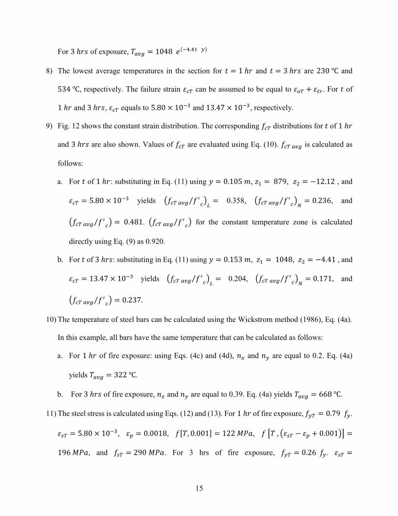
12) Using the steel and concrete stresses, the axial capacity of the example column is predicted as

2,618 𝑘𝑁 and 1,077 𝑘𝑁 after 1 ℎ𝑟 and 3 ℎ𝑟𝑠 fire exposure, respectively.

The steps mentioned above are repeated for the studied RC column at different fire durations.

The reduced axial capacity is estimated at each fire duration up to 3.75 ℎ𝑟𝑠, Fig. 13. Although the

proposed method results in conservative predictions, i.e. around 15% less than test results, it was

able to match the profile of degradation of the axial capacity and provided values with good

accuracy for design engineers. The proposed method can be applied to have a quick idea about the

structural fire safety of RC columns.

Validation

The proposed method is used to predict the axial compression capacity of three concentrically

loaded RC columns tested by Lie and Wollerton (1998); Dotreppe et al. (1997); and Hass (1986).

Lie and Wollerton (1998)

Table 2 shows the geometric and reinforcement properties of eighteen RC columns tested by

Lie and Wollerton (1998). All columns were axially loaded with a load 𝑃 and subjected to a

standard ASTM-E119 fire. Values for 𝑃 were kept constant during testing of all columns. The

fire endurance time (𝑡) was recorded at the end of each column test. The reinforcing steel cover

was 48 𝑚𝑚 for all columns except column NO. 16, where it was 64 𝑚𝑚. Fig. 14a shows a

comparison between 𝑃 , the predicted axial capacity using the method proposed in this paper and

17

the method proposed by Dotreppe et al. (1999) and applied by Tan and Tang (2004). The method

proposed in this paper provided good accuracy given the complexity of the problem.

Dotreppe et al. (1997)

Table 3 shows the properties of eight RC columns tested by Dotreppe et al. (1997). The

columns were loaded by the shown loads, 𝑃 . The heights of columns 1 to 3 and columns 4 to 8

were 3.90 𝑚 and 2.10 𝑚, respectively. All columns were exposed to a standard ISO 834 fire

exposure and the fire endurance (𝑡) for each column was recorded. The reinforcing steel cover was

25 𝑚𝑚 for all columns and the end conditions were pinned-pinned. Although all the loads were

concentrically applied at the beginning of the fire test, the columns were affected by buckling.

Dotreppe et al. (1999) proposed reducing the axial capacity by a buckling factor 𝜒(𝜆), Eq. (15).

𝜒(𝜆) = 1 − 𝜆 ≤ 20 (15a)

𝜒(𝜆) = 0.80.

20 < 𝜆 ≤ 70 (15b)

𝜒(𝜆) = 0.80.

70 < 𝜆 (15c)

where 𝜆 is the column slenderness ratio and 𝑐 is the concrete cover in 𝑚𝑚.

The predicted axial capacities by the proposed method are reduced by the factor 𝜒(𝜆). Fig. 14b

shows a comparison between applied concentric loads (𝑃 ) and the reduced axial capacity

predictions. The estimated axial capacities are in good agreement with the applied loads. Dotreppe

et al.’s method results in slightly better accuracy than the proposed method as shown in Fig. 14b.

This can be due to the fact that this method was calibrated using these experimental results.

18

Hass (1986)

Table 4 shows properties of seven RC columns tested by Hass (1986). All the columns were

subjected to a standard ISO 834 fire exposure. The reinforcing steel cover was 38 𝑚𝑚 and the end

conditions were pinned-pinned. The predicted axial capacities by the proposed method are reduced

by Dotreppe et al.’s buckling factor 𝜒(𝜆) to account for buckling (Dotreppe et al. 1999). Fig. 14c

shows a comparison between applied concentric loads (𝑃 ) and the predictions of the proposed

method. As shown in the figure, the proposed method underestimates the axial capacity of the tested

RC columns. A similar scatter in the results was found by Tan and Tang (2004) using Dotreppe et

al.’s method (1999). It should be noted that columns No. 1 and 2 have the same geometric, material,

and loading conditions but their fire endurance differs by 64%.

Limitations of the Proposed Method

Although the proposed method is simple and practical, it has the following limitations.

1) It does not account for concrete spalling. This assumption is only valid for normal strength

concrete (El-Fitiany and Youssef 2009). The spalling effect may be investigated by

reducing the fire exposed cross-section dimensions based on extent of spalling. The new

reinforcement cover, determined based on the new geometry, shall be used when

predicating the elevated temperature of the reinforcing bars.

2) It adopts a simple representation for transient creep strain in the constitutive stress-strain

relationship of concrete at elevated temperatures. This relationship is applicable for heating

rates between 2 and 50 𝐾/𝑚𝑖𝑛 (Eurocode 2-1992). For heating rates outside this range,

the reliability of using the proposed method should be investigated.

19

3) The buckling behavior can not be studied because of combined axial forces and flexural

moments.

Summary and Conclusion

This paper provides structural engineers with a rational tool to predict the axial compression

capacity of four-faces heated RC columns during fire events. The proposed tool can be applied

using a simple spreadsheet. The proposed method starts by dividing the analyzed section into

different temperature zones. Equations to evaluate the average temperature with each zone are

developed. The average temperature distribution is then used to estimate the failure strain.

Equations to evaluate the corresponding average concrete stress were developed by integrating the

concrete stresses along the height of the cross section. The failure strain is used to evaluate the

reinforcing bar stresses. The axial compressive capacity is then calculated by using the concrete

average stress and the reinforcing bar stresses. The errors resulting from different approximations

considered in this paper were found to be acceptable when evaluating the column axial capacity.

The proposed method is validated by comparing its predictions with the test results of thirty three

RC columns. A good agreement is found between the proposed method and the experimental

results. The presented work should be further validated for the parametric and natural fires based

on the available literature data.

Acknowledgments

This research was funded by the Natural Sciences and Engineering Research Council of Canada

(NSERC).

20

References Caldas RB, Sousa J, João BM and Fakurya RH (2010) Interaction diagrams for reinforced concrete

sections subjected to fire. Eng. Struct., 32(9), 2832–2838. Cement Association of Canada (2006) Concrete design handbook, CAN/CSA A23.3-04. 3rd Ed.,

Ottawa, ON, Canada. Dotreppe, JC, Franssen, JM and Vanderzeypen Y (1999) Calculation method for design of

reinforced concrete columns under fire conditions. ACI Struct. J., 96(1), 9-18. Dotreppe JC, Franssen JM, Bruls A, Baus R, Vandevelde P, Minne R, Nieuwenburg DV and

Lambotte H (1997) Experimental research on the determination of the main parameters affecting the behaviour of reinforced concrete columns under fire conditions. Mag. Concrete Res., 49(179), 117-127.

El-Fitiany SF and Youssef MA (2014) Simplified Interaction Diagrams for Fire-Exposed RC Columns, Eng. Struct., vol 70, pp. 246-259.

El-Fitiany SF and Youssef MA (2010) A Simplified Sectional Analysis Approach for RC Elements during Fire Events. 6th International Conference on Structures in Fire, Michigan State University, East Lansing, MI, 239-246.

El-Fitiany SF and Youssef MA (2009) Assessing the flexural and axial behaviour of reinforced concrete members at elevated temperatures using sectional analysis., FSJ, 44(5), 691-703.

El-Fitiany SF and Youssef MA (2011) Stress Block Parameters for Reinforced Concrete Beams During Fire Events. Innovations in Fire Design of Concrete Structures, ACI SP-279, 1-39.

Eurocode 2 (1992) Design of Concrete Structures. ENV EC2, Brussels. Hass R (1986) Practical rules for the design of reinforced concrete and composite columns

submitted to fire. Technical Rep. No. 69, Institute fur Baustoffe, Massivbau and Brandschutz der Technischen Universita Branschweig. (in German)

Law, A., and Gillie, M. (2010) Interaction Diagrams for Ambient and Heated Concrete Sections, Eng. Struct., 32(6), pp. 1641-1649.

Lie TT, and Woollerton J L (1998) Fire resistance of reinforced-concrete columns: Test results. Internal Rep. No. 569, National Research Council of Canada, Quebec, Canada.

Lie TT (1992) Structural fire protection. ASCE Manuals and Reports on Engineering Practice, no. 78, New York, 241 pp.

Lie TT, Lin TD, Allen DE, Abrams, MS (1984) Fire resistance of reinforced concrete columns. Technical Paper No. 378, Division of Building Research, National Research Council of Canada, Ottawa, Ontario, Canada.

NBCC (2005) National Building Code of Canada. National Research Council, Ottawa, ON. Raut N and Kodur VKR (2011) Modeling the fire response of reinforced concrete columns under

biaxial bending. ACI Struct. J., 108(6), 1-24. Tan KH, Tang CY (2004) Interaction Formula for Reinforced Concrete Columns in Fire

Conditions. ACI Struct. J., 101(1), 19-28. Terro MJ (1998) Numerical modeling of the behavior of concrete structures in fire. ACI Struct. J.,

95(2), 183-193. Wickstrom U (1986) A very simple method for estimating temperature in fire exposed concrete

structures. Fire Technology Technical report SP-RAPP 1986, 46, Swedish National Testing Institute, 186-194.

Youssef MA and Moftah, M (2007) General stress-strain relationship for concrete at elevated temperatures. Eng. Struct., 29(10), 2618-2634.

21

22

Tables and Figures Table 1–Parametric study cases

Col # b (𝑚𝑚)

h (𝑚𝑚)

f'c

(𝑀𝑃𝑎)

fy

(𝑀𝑃𝑎)

ρ % (Ag)

𝐶1 305 305 36.1 443.7 2.1

𝐶2 400 400 30 400 1.5

𝐶3 600 600 40 400 1.5

𝐶4 400 700 50 400 1.0

𝐶5 500 700 25 400 1.0

* all columns are analyzed up to 4 ℎ𝑟𝑠 of standard ASTM-E119 fire exposure Table 2–Details of Lie and Wollerton (1998)

No 𝑏

(𝑚𝑚) ℎ

(𝑚𝑚)

steel bars (𝑚𝑚)

𝑓

(𝑀𝑃𝑎)

𝑓

(𝑀𝑃𝑎)

𝑃

(𝑘𝑁) 𝑡

(𝑚𝑖𝑛)

1 305 305 4Ø25.5 36.9 444 1333 170

2 305 305 4Ø25.5 34.2 444 800 218

3 305 305 4Ø25.5 35.1 444 711 220

4 203 203 4Ø20.0 42.3 442 169 180

5 305 305 4Ø25.5 36.1 444 1067 208

6 305 305 4Ø25.5 34.8 444 1778 146

7 305 305 4Ø25.5 38.3 444 1333 187

8 305 305 4Ø25.5 43.6 444 1044 201

9 305 305 4Ø25.5 35.4 444 916 210

10 305 305 4Ø25.5 52.9 444 1178 227

11 305 305 4Ø25.5 49.5 444 1067 234

12 305 305 8Ø25.5 42.6 444 978 252

13 305 305 8Ø25.5 37.1 444 1333 225

14 406 406 8Ø25.5 38.8 444 2418 262

15 406 406 8Ø32.3 38.4 414 2795 285

16 406 406 8Ø32.3 46.2 414 2978 213

17 305 305 4Ø25.5 39.6 444 800 242

18 305 305 4Ø25.5 39.2 444 1000 220 * all columns have length (𝐿) of 3.81 𝑚 long

Table 3. Details of Dotreppe et al. (1997)

No 𝑏

(𝑚𝑚) ℎ

(𝑚𝑚)

steel bars (𝑚𝑚)

𝑓

(𝑀𝑃𝑎)

𝑓

(𝑀𝑃𝑎)

𝑃

(𝑘𝑁) 𝑡

(𝑚𝑖𝑛)

23

1* 300 300 4Ø16 33.9 576 950 61

2* 300 300 4Ø16 35.4 576 622 120

3* 300 300 4Ø16 29.3 576 422 116

4‡ 300 300 4Ø16 29.3 576 1270 63

5‡ 300 300 4Ø16 28.6 576 803 123

6‡ 300 300 4Ø25 26.2 591 878 69

7‡ 200 300 4Ø12 30.6 493 611 107

8‡ 200 300 4Ø12 27.3 493 620 97

* 𝐿 = 3.9 𝑚 ‡ 𝐿 = 2.1 𝑚

Table 4. Details of Hass (1986)

No 𝑏

(𝑚𝑚) ℎ

(𝑚𝑚)

steel bars (𝑚𝑚)

𝑓

(𝑀𝑃𝑎)

𝑓

(𝑀𝑃𝑎)

𝑃

(𝑘𝑁) 𝑡

(𝑚𝑖𝑛)

1* 300 300 6Ø20 24.1 487 930 84

2* 300 300 6Ø20 24.1 487 930 138

3‡ 300 300 6Ø20 34.1 487 880 108

4** 300 300 6Ø20 24.1 487 800 58

5* 200 200 4Ø20 24.1 487 420 58

6* 200 200 4Ø20 24.1 487 420 66

7‡ 200 200 4Ø20 24.1 487 340 48

* 𝐿 = 3.76 𝑚 ‡ 𝐿 = 4.76 𝑚 ** 𝐿 = 5.76 𝑚

24

x

y

h=305mm

b=305 mm

61 184 61

61

184

61Fire

( Left )

Fire

( Right )

Fire

( Upper )

Fire

( Bottom )

A = 4 - 25 mm

steel barss

heat transfer mesh

elements

A'

steel layer

concrete

s

A slayers

steel layer

Fire Fire

Fire

Fire

305 mm

305mm

Temperature ( oC )

300 600 900

He

igh

t (m

m)

0

75

150

225

300

T

Tavg

3 hrs1.0 hr

-1000

-500

0

500

1000

1500

Tem

per

atur

e (o

C)

b =

305

mm

h = 305 mm

steel bars

Fire (Bottom)

Fire (Upper)

Fire

(R

ight

)

Fire

(Lef

t)

100300

Fig. 1. Heat transfer analysis using FDM.

Fig. 2. Average temperature distribution.

b) 1 hr ASTM-E119 temperature contour. a) column section and mesh.

25

+ =

_ =

_ + 𝜀

_

𝜀

+ 𝜀

equivalent

linear strain

nonlinear

thermal strain

thermalstrain intop bars

thermalstrain inbottom bars

+

+

A's

A s

Fire Fire

Fire

Fire

b

h

Fig. 3. Sectional analysis approach for axially loaded RC sections exposed to fire.

c) equivalent linear thermal strain (𝜀 )

b) total strain (𝜀) d) equivalent mechanical strain (𝜀 )

f) nonlinear thermal strain (𝜀 )

a) fiber model

c) equivalent linear thermal strain (𝜀 )

e) self-induced thermal strain (𝜀 )

26

-15 -10 -5 0 5 10

Axi

al L

oad

(P )

x 1

03 (kN

)

0

1

2

3

4

5t = 0.0 hr

t = 1.0 hr

Axial Strain ( ) x 10-3

cT i

t = 3.0 hr

t = 3.0 hr

st is considered ( x 103 kN)

4000 8000 12000 16000

(st =

0.0

) (

x 1

03 k

N)

4000

8000

12000

16000

line of equality

Mean 0.952SD 0.028COV 0.029

T , Tavg ( x 103 kN)

4000 8000 12000 16000

T

= T

avg

( x

103 k

N)

4000

8000

12000

16000

line of equality

Mean 1.033SD 0.040COV 0.039

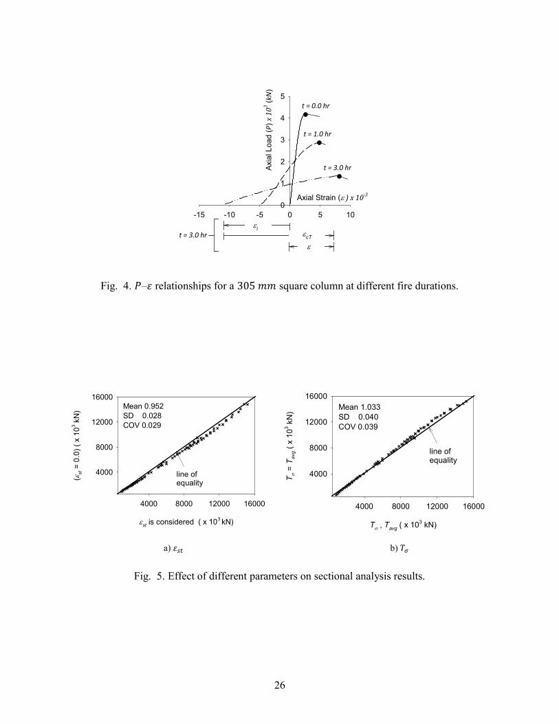
Fig. 4. 𝑃–𝜀 relationships for a 305 𝑚𝑚 square column at different fire durations.

Fig. 5. Effect of different parameters on sectional analysis results.

a) 𝜀

b) 𝑇

27

x

y

z

zR 1L , B

R 20 , B

R 1R , B

R 1L , 0

R 20 , 0

R 1R , 0

R 1L , T

R 20 , T

R 1R , T

z

zFire

( Left )

Fire

( Right )

Fire

( Top )

Fire

( Bottom )

area affectedby fire temp

area not affectedby fire temp

2

1

b

h

T avg 1

y = 0.0

y = z

Line 1-1

Line 2-2

T avg 1T avg 2

T avg 1 T avg 1T avg 2

R 1L , B

R 20 , B

R 1R , B

R 1L , 0

R 20 , 0

R 1R , 0

Fig. 6. Temperature calculation of example RC column (𝑧 ≤ 𝑏/2).

28

Line 1-1

y = h - z

Line 2-2

R 3L+R,T+B

T avg 1

y = 0.0

R 1L , B

R 3L+R, R 1

R , BB

L, T+BR 1

R, T+BR 1

Tavg 3

T avg 1

T avg 1

Tavg 3

T avg 1

x

y

z

L, T+B

zFire

( Right )

Fire

( Top )

R 1L , B

R 3L+R, R 1

R , B

R 1L , T

R 3L+R,

R 1R , T

T

B

R 1R, T+BR 1

Fire

( Left )

Fire

( Bottom )

2

1

b

h

R 3L+R,

T+B

z

z

Fig. 7. Temperature calculation of example RC column (𝑧 > 𝑏/2).

29

Tavg ( oC )

0 300 600 900 1200

oT

+

tr

0.00

0.02

0.04

0.06

0.08

Eurocode 2

Eq. (12)

Eurocode model for oT+ tr ( x 103 kN)

4000 8000 12000 16000

Eq.

(8

) fo

r o

T+

tr (

x 1

03 kN

)

4000

8000

12000

16000line of equality

Mean 0.966SD 0.046COV 0.048

Eurocode f 'cT siliceous ( x 103 kN)

4000 8000 12000 16000Eu

roco

de

f ' cT

ca

rbo

nat

e (

x 1

03 k

N)

4000

8000

12000

16000

line of equality

Mean 1.076SD 0.060COV 0.055

Fig. 8. Variation of 𝜀 + 𝜀 at elevated temperatures.

Fig. 9- Effect of different parameters on sectional analysis results.

a) proposed Eq. (8)

b) aggregate type

30

x

y

305mm

305 mm

Fire

( Left )

Fire

( Right )

Fire

( Upper )

Fire

( Bottom )

Tavg ( oC )

0 400 800 1200

He

ight

(m

m)

0

75

150

225

300

FDM [1]

ModifiedWickstorm

1 hr

3 hrs

cT x 10-3

0 3 6 9 12 15 18

f cT /

f ' c

0.00

0.25

0.50

0.75

1.00

oT + tr = 5.58 x 10-3

Tavg = 230 oC400 oC

600 oC

Fig. 10. Concrete stress-strain relationship at different 𝑇 values.

Fig. 11. 𝑇 distribution of the example RC column.

b) 𝑇 dist a) four-face heated RC section

31

𝜀

x

y

305

305

Fire

( Left )

Fire

( Right )

Fire

( Upper )

Fire

( Bottom )

f cT / f 'c

0.0 0.5 1.0

He

igh

t (m

m)

0

75

150

225

300

0.48 f 'c

0.92 f 'c

0.48 f 'c

y

f cT / f 'c

0.0 0.5 1.0

0.24 f 'c

y

Fire duration (min)

0 60 120 180 240

Axi

al C

apa

city

x 1

03 (

kN)

0

1

2

3

4 Test Lie et al. (1984)

Sectional method

Proposed method

Fig. 12. Average compression stresses distribution.

Fig. 13. Axial capacity predictions of example column.

b) 𝜀 dist. a) four-face heated RC section

d) 𝑓 dist.. (𝑡 = 3.0 ℎ𝑟𝑠)

c) 𝑓 dist.. (𝑡 = 1.0 ℎ𝑟)

32

Applied load x 103 (kN)

0 1 2 3 4

Pre

dic

ted

cap

acity

x 1

03 (

kN)

0

1

2

3

4

line of equality

Lie and Wollerton (1998)Mean 1.117SD 0.294COV 0.263

Applied load x 103 (kN)

0.0 0.2 0.4 0.6 0.8 1.0

Pre

dict

ed c

apa

city

x 1

03 (

kN)

0.0

0.2

0.4

0.6

0.8

1.0

line of equality

Hass (1986)Mean 0.877SD 0.258COV 0.295

Applied load x 103 (kN)

0.0 0.2 0.4 0.6 0.8 1.0 1.2 1.4

Pre

dict

ed

capa

city

x 1

03 (

kN)

0.0

0.2

0.4

0.6

0.8

1.0

1.2

1.4

line of equality

Dotreppe et al. (1997)Mean 0.782SD 0.140COV 0.179

Applied load x 103 (kN)

0 1 2 3 4

Pre

dic

ted

ca

paci

ty x

10

3 (

kN)

0

1

2

3

4

line of equality

Lie and Wollerton (1998)Mean 0.747SD 0.160COV 0.213

Applied load x 103 (kN)

0.0 0.2 0.4 0.6 0.8 1.0 1.2 1.4

Pre

dic

ted

cap

acity

x 1

03 (kN

)

0.0

0.2

0.4

0.6

0.8

1.0

1.2

1.4

line of equality

Dotreppe et al. (1997)Mean 0.905SD 0.228COV 0.252

Applied load x 103 (kN)

0.0 0.2 0.4 0.6 0.8 1.0

Pre

dict

ed

capa

city

x 1

03 (

kN)

0.0

0.2

0.4

0.6

0.8

1.0

line of equality

Hass (1986)Mean 0.705SD 0.134COV 0.190

Proposed method Tan and Tang [18]

Fig. 14. Proposed method predictions for different experimental works.

a)

c)

b)