Energy Conservation In The Crushed Stone Industryinfohouse.p2ric.org/ref/33/32450.pdf · ·...

:

ENERGY MANAGEMENT GUIDELINES

nsa National Stone Association

REPRINTED JUNE 1992

1988 Review and Update This Energy Conservation Manual was written in 1978 by a group of well-informed individuals who were very

close to the energy issues at that time. Ten years have passed since the manual was completed and it became incumbent on the Automation Committee to review this manual. Our review indicated that the manual was very well written and the substance of it did not in any way require corrections of any nature. We felt that the basic principles relating to electricity and diesel and the applications of these energies were well defined and we should only try to build on this foundation rather than attempt otherwise.

In the last 10 years, natural gas has become an economic factor in the heating and drying area to the extent many operators are or should be involved in the alternate fuel management program. Energy management of operations in conjunction with redesigned electrical rate structures has become a real challenge.

In our effort to make this manual a resource tool for the members of NSA we have included:

An example of demand management. Cross comparison of various fuels to natural gas for alternate fuel use consideration. A listing of available energy groups. and state stone associations. Characteristics of lubricants to help in proper application. Update on diesel versus electric to reflect present costs. A diagram of an energy management system. Various forms that could assist in your energy analysis. Several examples of using the energy management guidelines.

We hope this updated manual will become an important part of your library. If you feel other aspects to energy

The committee members involved in this update were: considerations should be added or modification made, we welcome comments.

Steve Gregory, Vulcan Materials Company George B. Brewer, Florida Rock Industries, Inc. Robert Martin, Marttec, Inc. Winfield E. Rogers, Genstar Building Materials

TABLE OF CONTENTS

INTRODUCTION

SECTION I HOW TO ANALYZE YOUR PRESENT ENERGY USAGE

A. Audit Goals B . Assigning Responsibility C. Setting Up an Audit D. Using the Information E. Sample Audit Forms F. Utility Verification Record

SECTION 11 WAYS TO CONSERVE ENERGY

A. General Practices B . Electrical Facilities

1. Power Source 2. Electric Motor Application 3. Power Factor 4. Instrumentation 5. Electric Motor Design

C. Diesel Equipment , 1. Plant Production Facilities 2. Diesel-Powered Mobile Equipment

1. General 2. Distance 3. Pump and Fan Design Considerations 4. Pipeline Capacity

E. Lighting F. Grease Application Guide G. Energy Management Systems

D. Pump and Fan Systems

SECTION III WAYS TO SAVE ON ENERGY COSTS

A. Electrical Systems 1. Rate Structure 2. Primary Metering 3. PeakDemand 4. Power Factor

B. Diesel Versus Electric C. Lighting D. Natural Gas Versus Other Fuels

SECTION IV INDUSTRIAL ENERGY GROUPS AND STATE STONE ASSOCIATIONS

SECTION V ENERGY PUBLICATIONS

SECTION VI EQUATIONS, FORMULAS, CONVERSION FACTORS

SECTION VII DEMAND AND ENERGY SAVINGS

SECTION VIII IMPLEMENTING THE ENERGY MANAGEMENT PROGRAM

PAGE

1

1-1 to 1-8

I- I I- 1 1-1 to 3 1-3 1-4 to 6 1-7 to 8

11-1 to 11-34

II- 1 11-2 to 22 11- 1 11-2 to 3 11-3 to 14 11-14 to 16 11-16 to 22 11-22 to 24 11-22 11-22 to 24 11-24 to 27 11-24 11-24 11-25 to 26 11-26 to 27 11-27 to 30 11-30 to 31 11-31 to 34

111- 1 to 111- 15

nI-1 to 7 HI-1 to 4 111-5 111-5 to 6 111-6 to 7 111-7 111-7 111-7 to 15

IV-1 to IV-5

v-1 to v-2

VI-1 to VI-3

VII-1 TO VII-17

VIII-1 TO VIII-19

INTRODUCTION Just a few short years ago this country had an abundance of low cost energy. Today as a nation we have to

pay the price of a changing world situation. Energy consumption continues to grow and costs continue to escalate. The situation promises to get no better and, as a nation, we must not wait until tomorrow to accept this fact of life. While our current dilemma is the availability of inexpensive energy, our ultimate problem will lie in the availability of energy at any price. The alternatives are to act now to conserve what we have and develop new sources of

Not everyone can develop these new sources of energy for the future but everyone can help conserve what we now have and use. Energy conservation is a common term today, unheard of 10 years ago.

Since industrial, commercial and transportation business activity accounts for almost 70 percent of total energy consumption in the United States, the business community in general is in an important position to contribute to a reduction in the seriousness of the problem.

Why should industry do anything to conserve energy? There are two obvious reasons. One is our national interest-work together for the common cause. The other, which has more tangible meaning, is profit. Every dollar reduced from present energy costs falls directly to the bottom line. Profit-central to the free enterprise system that molded our progress, is the same motivation that will help us in our current energy dilemma. These two reasons, national survival and profit, are unbeatable.

With this as a basic concept, it becomes fairly obvious that conservation through energy management is no different than the application of the same basic techniques, applied to the use of energy, that would apply to administration, finance, marketing, purchasing and production in any well-run business venture.

Can it be done? Can we do it? The answer is yes. Much has been written on progress made by many major energy-intensive industries, But these corporate giants have large staffs with energy administrators and coordinators. Nevertheless, even without this advantage any organization, once committed to a program, can achieve results through a planned approach. The results will be limited only by your commitment and innovation.

This manual is intended to outline for you how to go about conserving energy. It is intended to help you develop a specific, real world plan of action to reduce the money you spend on energy without reducing your capacity or efficiency. It will outline how to conduct an energy survey or audit. You must know where you are before you know where you want to go. From this, beginning suggestions on analyzing opportunities, evaluation and making recommendations, organizing, managing, monitoring and action planning will be outlined.

Once you are really committed to the program, the only thing that will surprise you are the opportunities that lie within your reach.

supply *

1

SECTION I ANALYZE YOUR PRESENT USAGE

A. Audit Goals Assigning Responsibility Setting Up an Audit Using the Information Sample Audit Forms Utility Verification Record

I- 1 I- 1 1-1 to 3 1-3 1-4 to 6 1-7 to 9

SECTION I: ANALYZE YOUR PRESENT USAGE In order to initiate an energy conservation program it is necessary to determine what energy is being consumed,

how and where. Since we are really looking to reductions in energy consumption to save money, we’ll use the financial term

“audit” for this process. We find that in many cases our accounting systems are not set up for this kind of audit, however, and it becomes necessary to start from scratch.

A. Audit Goals

1) To pinpoint equipment that operates inefficiently and locate specific energy “leaks.”

2) To identify energy saving opportunities and allow their translation into projects.

3) To calculate the energy cost of various operations and to determine the cost saving potential associated with each project.

4) To assign priorities to the various energy saving projects or study areas.

B. Assigning Responsibility

The responsibility for conducting an energy audit, and following through with energy conservation projects or practices will be assigned to various positions in different organizations. Whether it requires one person or a team, be it a full-time responsibility or an add-on to an existing job, the person(s) assigned must:

1) be aware of the dollar value of conserving energy;

2) have the commitment of top management; and

3) understand the basics of energy technology and the operations of the facilities.

C. Setting Up an Audit

It would be impossible to set up an energy audit that would fit everyone’s needs. There are, however, three guidelines which should apply to most operations:

1) Production equipment (any equipment that operates when you are producing a product and does not operate when you are not producing) should be separated from non-production equipment.

2) Separate processes should be monitored separately. In addition, processes making different products at different times should be monitored so that the energy consumption for each product line is reported separately.

3) Since the various types of energy consumed (electricity, gas, oil, gasoline, etc.) have different amounts of energy per unit, the units should be converted to a common base. Sooner or later you may want to compare electric versus diesel, etc. in deciding which type of equipment to buy.

The standard energy unit in the United States is the BTU (British Thermal Unit), which is defined as the amount of heat required to raise the temperature of one pound of water from 59.5”F to 60.5”F. Figure I- A shows approximate energy content of various energy sources, if your suppliers cannot give you an exact number.

For a first round comparison, an analysis of overall energylton data is meaningful. It is necessary to select a period of time as a basis of study. A month is most convenient since this represents

thausual billing period. One caution-the billing periods do not necessarily coincide with the calendar month. Care must be exercised to use the same starting and stopping period when measuring usage of more than one energy source.

1- 1

Energy Source Units Conversion

Electricity* Coal (Bituminous) Natural Gas Oil - No. 6

No. 4 No. 2 No. 2 Diesel

Kerosene Gasoline L-P Gas, Propane

Kilowatt Hour (KWH) Tons

Thousand Cubic Feet (MCF) Barrel (BBL) 42 G/Barrel

Gallon Gallon Gallon Gallon Gallon Gallon Gallon

3412 BTU/KWH 25-28 Million BTU/Ton 1.03 Million BTU/MCF 6.3 Million BTU/BBL 150,000 BTU/GAL 144,000 BTU/GAL 138,000 BTU/GAL 138,000 BTU/GAL 135,000 BTU/GAL 125,000 BTU/GAL 95,000 BTU/GAL

*The energy value of electricity is the value the consumer receives when using it. To produce 1 KWH of electricity requires approximately 10,500 BTU/KWH.

FIGURE I-A ENERGY CONVERSION UNITS

To complete the analysis the only other information needed is the actual usage of energy by source for the selected study period. This is best accomplished using meters that are read at the beginning of each period, or in finite increments as in the case of mobile fuel delivery. In cases where the energy source is stored (example: coal or fuel) add deliveries to beginning inventory, then subtract ending inventory to obtain consumption.

With the above information, an audit of the overall energy usage can be prepared. This can be reduced to usage per ton of production by dividing the production matching the study period into the total energy usage figure.

A sample Energy Use/Cost Report form, Figure I-B, gives the minimum amount of information necessary for management to trace energy costs and energy use efficiency. For many plants, a form similar to the sample copy (with changes to reflect the local situation, e.g., eliminating the unused fuel categories) would be adequate. However, in cases where different products requiring significantly different amounts of energy are being produced, single forms should be used for each such product. Examples of such cases might be where parts of the products are dried or where some of the product goes through the primary crusher only, while another portion goes through a secondary crushing process. To set up energy forms on a product basis, it is only necessary to allocate per ton of product the energy used in common to produce all products and then add for each product any extra energy required, (e.g., gas for drying or secondary crusher KWH). Carrying out the analyses product by product also ensures that the additional energy costs to produce a particular product are actually being recovered in the selling price.

An alternate approach to energy audits is to arrange the fuel usage and cost by function-for example, loading, transferring to crusher, crushing, screening, distribution, etc. This approach is actually more desirable since an increase in energy costs for a particular area would become immediately evident, allowing timely action to be taken. With the product-by-product approach, increases might not be noticed immediately. The problem with functional auditing is that considerable additional time and record keeping and the installation of individual meters would be required, expenses that might not be justified in many cases. Nonetheless, each plant should select particular pieces of equipment using large amounts of energy for functional audits. The audit can save money if it reveals, for example, that the KWWton for the crusher are rapidly increasing or the fuel usage per hour for a front-end loader has increased.

Comparisons of these figures monthly can be helpful in alerting you to wasteful practices. Likewise, comparison to industry-wide figures will give you an indication of your overall efficiency.

Care should be exercised in comparing different operations, however. Major variables affecting consumption include stripping methods and volume, haulage lengths, grades, pit water quantity and pumping height, rock hardness and toughness, and product sizing.

The Energy Committee has developed some figures for member plants, however, which should give you an idea if you are in the ballpark. The data ranged from 20,000 BTU/ton for a concrete stone plant to 54,000 BTU/ ton for a plant producing fine agricultural limestone as well as graded stone. The average for approximately 20 plants was 33,500 BTU/ton, excluding blasting.

Once you have determined the BTU/ton produced, your audit should be continued to check power factor and power demand. Power factor is an indication of how much of the voltage and amps the utility sells you are actually doing work. It is a rather complex item, and is lower than unity due to losses in motor windings, etc. A power factor of 1 .O would be ideal, but normally impractical. Most utilities measure KWH and power factor, and charge

1-2

a penalty if the power factor is below a given level (usually 0.85 or 0.90). In these cases, you should consider the use of capacitors or other means to correct your power factor to above the penalty levels. In some cases, the utility will meter KVA directly and your penalty becomes the purchase of extra KVA to accomplish the work your motors do with KWH, and correction to higher power factors may be indicated. Power factor correction will be discussed further on in this handbook.

The power demand charge is included in almost every industrial rate, and is a charge for the maximum amount of power you require in a given month for a short period of time (usually 5, 15 or 30 minutes). In some cases, your maximum or peak demand may be applied for the next full year.

For example, let’s assume a plant which normally operates at 2,000 KW, with a 15-minute demand period. If that plant were able to maintain that maximum level for the entire billing period, their demand charge would be based on 2,000 KW. If the plant, for some reason, drew 2,300 KW for only 15 minutes during the month, its demand charge for the month would be based on 2,300 KW. At $3.00/KW, the penalty for that 15 minutes use of an extra 300 KW would cost $900, and in many contracts would also increase the energy portion of the power bill.

Both power factor and demand meters can be purchased or rented, and may be available from your utility if you do not presently meter these items. Reduction of peak demand and power factor improvement can save considerable energy dollars. See Sections I1 and 111 for further discussion of these topics.

After this first rough comparison, the information developed in the audit can be used to begin isolating energy gulpers-areas where high usage, low power factor, etc., flag high potential for savings. Priorities should be established, listing in order of potential savings (or in ease of obtaining results) each area of the plant.

Beginning with an area selected after the general audit, a unit-by-unit survey of each piece of electrically driven equipment is performed, using a survey form similar to Figure I-C at the back of this section. Each unit is checked for actual consumption compared with rated consumption. A large discrepancy indicates that corrective action should be taken.

A similar survey can be run for mobile equipment and diesel sets. Hourly fuel consumption is checked against manufacturers’ data and other similar vehicles; differences indicate potential problems and cost reduction possibilities.

This step is time consuming, but well worth the effort. In addition to flagging energy wasters (or showing proper sizing and operation) the survey has value in two ways. First, you now have a detailed record of every motor in the plant, useful during breakdown emergencies and the like. Second, you have an operating data base to refer to when future problems or modifications arise, which can be invaluable for troubleshooting.

D. Using the Information

With the information gained in the audits, you are now well informed on your energy consumption, and can begin to take steps to reduce it. The following sections of this handbook are to assist you in making the changes in equipment or operating methods required to obtain the best operation of your equipment at the least cost for energy.

1-3

Monthly Energy UseKOst Report

CONVERSION FUEL

Electricity

Diesel Oil

#2 Oil

Gasoline

Natural Gas

Propane or LPG

Others

TOTALS

Production Tons: Month YTD

Energy Cost Per Ton: Month YTD

MBTU Per Ton: Month YTD

Definitions: MBTU = 1000 BTU MCF = 1000 Cubic Feet P.U. = Purchase Unit (tons coal, etc.)

Figure 1-6

1-4

ELECTRIC ENERGY AUDIT FORM

x

* COI (1) x 0.746; (HP x 0.746 = KW) ** Col (6) x Col (5) X 1.732 x P.F. + 1000 = KW

(If P.F. not known, use 0.9) *** Actual operating data is more meaningful, in energy studies, if one takes no load, average load, and full load readings.

Figure I-C

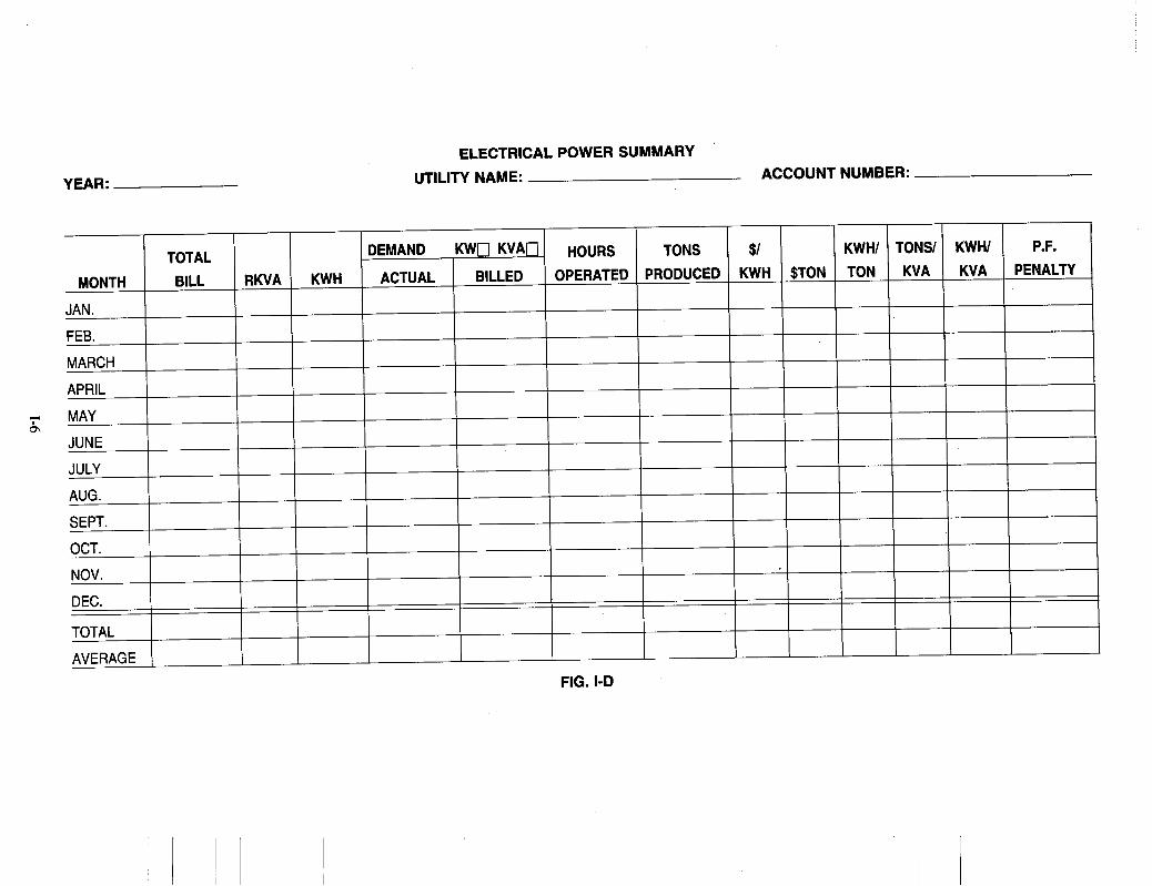
YEAR:

P.F. TOTAL DEMAND KWO KVAU HOURS TONS $1 KWH/ TONS/ KWH/

MONTH BILL RKVA KWH ACTUAL BILLED OPERATED PRODUCED KWH $TON TON KVA KVA PENALTY

JAN.

FEB.

MARCH

APRIL

MAY

JUNE

JULY

AUG.

SEPT.

OCT.

NOV.

DEC.

TOTAL

AVERAGE

z

p- -- p-

--- ---

ELECTRICAL POWER SUMMARY UTILITY NAME: ACCOUNT NUMBER:

-

F. Utility Verification Record Instructions

The instructions for filling out and using the attached utility verification are very simple:

1. Fill out the blanks for date, plant, utility name and account number (from power bill) on the f i s t page.

2. Put your return address, as indicated, on the second page. 3. Mail it to your local utility.

Fill in other blanks if known.

The information you receive from your utility can be most valuable in evaluating areas of potential savings. Many utilities will not be capable of furnishing the information requested on this form. Most of the larger utilities, however, will have this information available, but only if you request it. If nothing else, this request form will serve as an indication of your interest in reducing power cost and your desire to have the utility assist you in this matter. It would also be advisable to set up an appointment with your utility representative to review the information being requested.

UTILITY VERIFICATION RECORD Date:

Plant:

Utility name: Address:

Account no.:

Utility representative: Phone no.: (-)

Contract date: Current rate schedule:

Power factor clause: (yes, no) Average power factor:

Service (Primary, Secondary) Voltage: Primary

Secondary

No. of meters at this location: Demand basis (KW, KVA)

Highest demand past 12 months:

Minimum power factor to avoid penalty:

Month Demand KWH

Demand interval: (15 min., 30 min.) Sliding window: (yes, no)

A. Which of the following information appears on monthly bill?

c] KWH c] Power factor

c] KW (Billed) KW (Actual)

KVA (Billed) 0 KVA (Actual)

c] RKVA Power factor penalty

B. Is there a ratchet associated with this rate schedule? (yes, no)

1-7

C. How is monthly power factor determined?

0 Power factor at peak demand

0 Average power factor for billing cycle

0 Average power factor at three (3) highest peak demands

0 Power factor calculated using RKVA at highest peak demand

0 Other

If other, please explain:

D. Are mag-tape printouts available?

E. Is there a discount for primary metering? If yes, what is the discount?

F. Please attach the following information: 1. Load profile of monthly demand 2. Previous 12 month history 3. Copy of current rate schedule 4. Current fuel adjustment or fuel cost recovery charge 5 . Copy of effective contract 6 . Minimum bill calculation 7. How demand is determined 8. Copies of all rate schedules available, including all available rate riders, such as off-peak, time-of-use,

(yes, no)

(yes, no)

intermptable, supplemental energy, etc.

I verify, to the best of my knowledge, that this facility is currently being billed on the most economical rate available.

Utility Representative Date

Retum to:

1-8

SECTION 11 WAYS TO CONSERVE ENERGY

Page

A. General Practices

B. Electrical Facilities 1. Power Source 2. Electric Motor Application

a) Crushers b) Screens c) Conveyors

3. Power Factor 4. Instrumentation 5 . Electric Motor Design

a) Insulation Class b) Ambient Temperature c) Temperature Rise d) Service Factor e) NEMA Design Type f) Power Factor and Efficiency g) System Voltage and Frequency Variation

C. Diesel Equipment 1. Plant Production Facilities 2. Diesel-Powered Mobile Equipment

a) Vehicle Selection 1) Match equipment to your operation 2) Proper gearing ratios 3) Automatic transmissions

1) Keep engine tuned 2) Keep fuel clean 3) Pay attention to tire performance 4) Preheat cold engine

b) Maintenance

c) Payload

D. Pump and Fan Systems 1. General 2. Distance 3. Pump and Fan Design Considerations 4. Pipeline Capacity

E. Lighting F. Grease Application Guide G. Energy Management Systems

11- 1

11-1 to 22 II-1 to 2 11-2 to 3 11-2 11-2 to 3 II-3 11-3 to 14 11-14 to 16 11-16 to 22 11- 16 11- 16 11-16 11-16 to 18 11-18 to 19 11-19 to 21 11-22

11-22 to 24 11-22 11-22 to 24 11-23 11-23 11-23 11-23 11-23 to 24 11-23 11-24 11-24 11-24 11-24

11-24 to 27 11-24 11-24 to 25 11-25 to 26 11-26 to 27 11-27 to 30 11-30 to 31 11-31 to 34

!

i

SECTION 11: WAYS TO CONSERVE ENERGY

A. General Practices

1) Energy is defined as the capacity to do work. Work can be further defined as the application of a force over a distance. With these in mind any revision in equipment or procedures that would result in a reduction in the force applied or in the distance involved (be it horizontal or vertical) results in energy conservation.

2) Housekeeping-Obviously clean, well-lubricated equipment performs more efficiently than does equipment covered with rust, corrosion, and dirt.

3) Distances-Total energy usage for an operation involves the distance stone travels from the quarry face to the scale house. Therefore, relocating stockpiles relative to plants, or plants relative to quarry faces only alters the energy distribution within the operation. Conversely, opening deeper lifts or faces further from the crushers increases energy requirements.

Energy can be conserved by careful layout of a quarrying operation, and these savings accumulate for the life of the operation. Therefore, it behooves operational management to be conscious of distance when developing plans.

4) Consistency-Equipment manufacturers are generally in agreement that their equipment works most efficiently under uniform loading. It follows then that any practice that would tend to eliminate peaks and valleys would conserve energy.

a) Sensors-Sensors that measure performance and then cause reaction to wide variances in performance are helpful in smoothing out surges. Ammeters, speed measuring devices, and weighing devices all fit in this category.

b) Surge Piles-In any production line the rate of production is only as high as its weakest unit. When one unit malfunctions, it affects overall performance.

By use of surge piles with corresponding recovery methods, the impact of a breakdown or even slowdown of any one part of the production line is minimized. Surge piles of crushed material within the production line use tunnels with feeders for reclaiming the material. Surges of shot rock prior to the crusher can be reclaimed using large front-end loaders. In either case the net effect is to keep the feed rate consistent, improving production rates and minimizing the energy requirement per ton of production.

5) Operate at Full Capacity-The most efficient use of energy for any equipment that converts an energy source into mechanical movement occurs when that equipment operates at full capacity. This applies regardless of energy source.

With this in mind it is important to size all phases of production to meet the same rate of production. Designers then must be very careful in reacting to other design considerations such as capital cost, startup loading, weather conditions, availability and market fluctuations.

B. Electrical Facilities

Electricity as an energy source has many desirable features but several factors must be recognized.

1) Power Source-The source of generation is important. If supplied by a power company, the availability is 100 percent unless a general system failure occurs, as has happened on several occasions in recent years on the east coast. However, energy purchased in this form is expensive because all the hidden costs of generation and distribution are included.

On-site generation using diesel generators is an option. If the cost of fuel is the only cost recognized, this means of providing electric energy is only a fraction of the cost of buying electricity from a power company. Lest this imbalance becomes misleading, the operator is cautioned to recognize the very real and significant presence of other costs that sometimes do not get included. These other costs include the ownership and

11- 1

operating costs for the diesel generators. And even more significant is the cost of downtime. If the profit that could have been realized during that downtime is added to the fuel, ownership, and operating costs, the initial advantage of on-site generation when considering energy purchase only quickly disappears. The cost of on-site diesel generation is explored in Section 111.

The question is frequently asked which option uses more energy. There appears at this time to be no significant difference.

Electric Motor Applicufiion-The properly applied induction motor should develop enough starting torque to start the machine to which it is connected, accelerate this machine in a reasonably short time to rated speed, and continuously drive the machine efficiently. It is not always easy to get acceptable performances with all three requirements satisfied. Motor characteristics are such that the most efficient operation occurs near rated load horsepower, but machine characteristics often require high starting torques and low running torques. These high starting torque requirements occur on loaded equipment. Operqting personnel find it undesirable to unload the machine by hand (thereby reducing torque requirements to within motor capabilities). Therefore, a motor large enough to develop starting torque for any load condition is often chosen to drive the machine. This results in the motor being lightly loaded at rated speed and in turn, it operates less efficiently. This type of motor application can be kept to a minimum by fully understanding how to choose a motor with the proper characteristics to drive a machine.

Electric motor characteristics are also important to proper application. Starting and maximum torque, service factor, speed, relative wk2 (inertia) at motor shaft, and bearing type are some factors to be evaluated for each operation. Should the motor be squirrel cage or wound rotor induction type or synchronous? These questions must be answered after careful study.

Optimum electrical power application and utilization is dependent on proper selection of (1) product sizes to meet specification, (2) type of crushing (jaw, cone, gyratory) to reduce over crushing, (3) adequate screening, (4) stockpile size and location, (5) number of hours, and (6) time of day for operation.

a) Crushers-Horsepower consumed in any crushing operation is directly proportional to tons per hour, to the hardness or crushability of the ore, and to the ratio of reduction (ratio of topsize of feed to topsize of product). A common measure of power usage is HP/ton or KWWton. The lower this number, the better the energy efficiency.

Because of the size requirements, crusher motor application commands special emphasis. Certain characteristics that relate to resistance to crushing of material, whether stone or ore, must be known prior to determining horsepower requirements. These include the “crushability” of the feed, often referred to as toughness, friability or hardness of material. These factors are difficult to evaluate without proper testing because the same material type will differ in various locations. One method to determine HP requirements is to perform actual crushing tests on the feed material using a pilot crushing circuit. Crusher motor power draw can be recorded directly in KWH per ton. This method involves availability of from several hundred pounds to several tons of crusher feed material and hence can be quite time consuming and costly.

The Bond Twin Pendulum Crushability Test,* a more common and much less expensive method, establishes the impact crushability of quarried rock, stone or ore. In these tests, approximately 20 to 30 representative pieces, passing 3 inch and retained on 2 inch, are subjected to impact by swinging pendulums. The energy required to completely fracture the specimen tested is used to determine a Work Index. Using the standard Bond Energy Formula,* which takes into account the ratio of reduction of the feed (ratio of feed size to product size), a close approximation of total HP required can be determined using proposed crushing rate in tons per hour for gyratory, jaw and cone crushers.

In the absence of a Work Index test, initial power estimates can be made by comparing data for a proposed project with operating conditions at similar installations.

*Crushing and grinding calculations, by Fred C. Bond, Sr. Staff Engineer, Process Machinery Department, Allis-Chalmers Manufacturing Company, January 2, 1961.

11-2

b) Screens-Screen horsepower requirements are primarily based on torque needed to effectively start the screen vibrating mechanism. These requirements are essentially a function of live weight of the screen as well as speed and amplitude (throw). Therefore, proper screen size (weight) selection is essential to proper horsepower requirements. Screen operating horsepower is about 50 to 75 percent of starting horsepower due to the high starting torque required.

c) Conveyors-For belt conveyors, the power required for proper operation depends primarily on the maximum tonnage handled, the length of the conveyor, and the vertical distance that material is lifted. Additional power considerations include friction from idlers, loading hoppers, belt scrapers, take-up, etc .

Another important consideration in the application of motors for operation of processing equipment in the aggregate industry is that of “over crushing,” or “over screening.” Too close a crusher setting may result in too many fines or waste. Too much screening area wastes space, power and capital costs. Too large a crusher (for tonnages processed) results in inefficiency through low reduction ratios and improper sizing of product.

In summation, those factors discussed above as well as other intangible elements must be carefully analyzed and reviewed by the energy conscious operator. Remember that the suppliers of crushers, screens and conveyors have the technical expertise to apply motors properly if application data is provided them. In essence, the more information the equipment supplier has regarding the application and type operation, the more accurate will be the motor application and the greater the efficiency of the operation.

3) Power Factor-Electric power factor is an important yet difficult concept for laymen to understand. However, because it does affect energy consumption and costs, it must be considered.

Lewis Pettinos, in his address to the joint NSGA-NRMCA session in February 1976 in Houston, discussed power factor as follows: “Poor power factor is caused by operation of any inductive device-that is, any alternating current component on the principle of magnetism. In an inductive component, current flow can be compared somewhat to action of waves on a beach. First, there is an inrush (useful current). This is followed by a rush of current out of phase with the voltage, producing no useful work. Yet this out-of- phase current produces a very real heating effect, and must be considered in sizing transformers, distribution and transmission conductors, and even the generating equipment far away at the utility’s generating plant.”

Power companies add on the penalty of power factor because they have to furnish power equipment, lines and so forth, which are of higher capacity than actually used. Since motors usually make up the largest single use of electrical energy at a plant, and since most are induction motors, it is not too unusual to find overall uncontrolled power factors as low as 60 to 70 percent.

Thus, if a plant is operating with an electrical load of 300 kilowatts with a low power factor of 60 percent, the total electrical power that has to be transmitted is 300 divided by decimal .60 or 500 KVA. This means that the entire electrical distribution system must now carry 500 KVA to deliver 300 KW of useful power to the point of application. This results in direct energy loss, and can overload the wiring system. To illustrate how much low power factor increases the load on the system, consider the following: “If four identical induction motors operate with an average power factor of 75 percent, then correcting the power factor to 94 percent leaves enough system capacity to carry a fifth motor.”

Power factor is said to be “high” or ‘‘low’’ and “leading” and “lagging.” Power factor is generally said to be high if it is 90 or 95 percent. Anything below 80 percent is considered low.

The leading and lagging aspects of PF are dependent on the electrical system’s inductive or capacitive reactance. Industrial loads such as induction motors, transformers, and fluorescent lighting have a lagging power factor. Synchronous motors and capacitors have leading power factors. Although some individual machines may have leading PFs, it is generally desirable for a system to have a high lagging PF. Low PF is bad primarily for three reasons:

a) low PF causes high load current, which must be supplied by the power company. This requires the

11-3

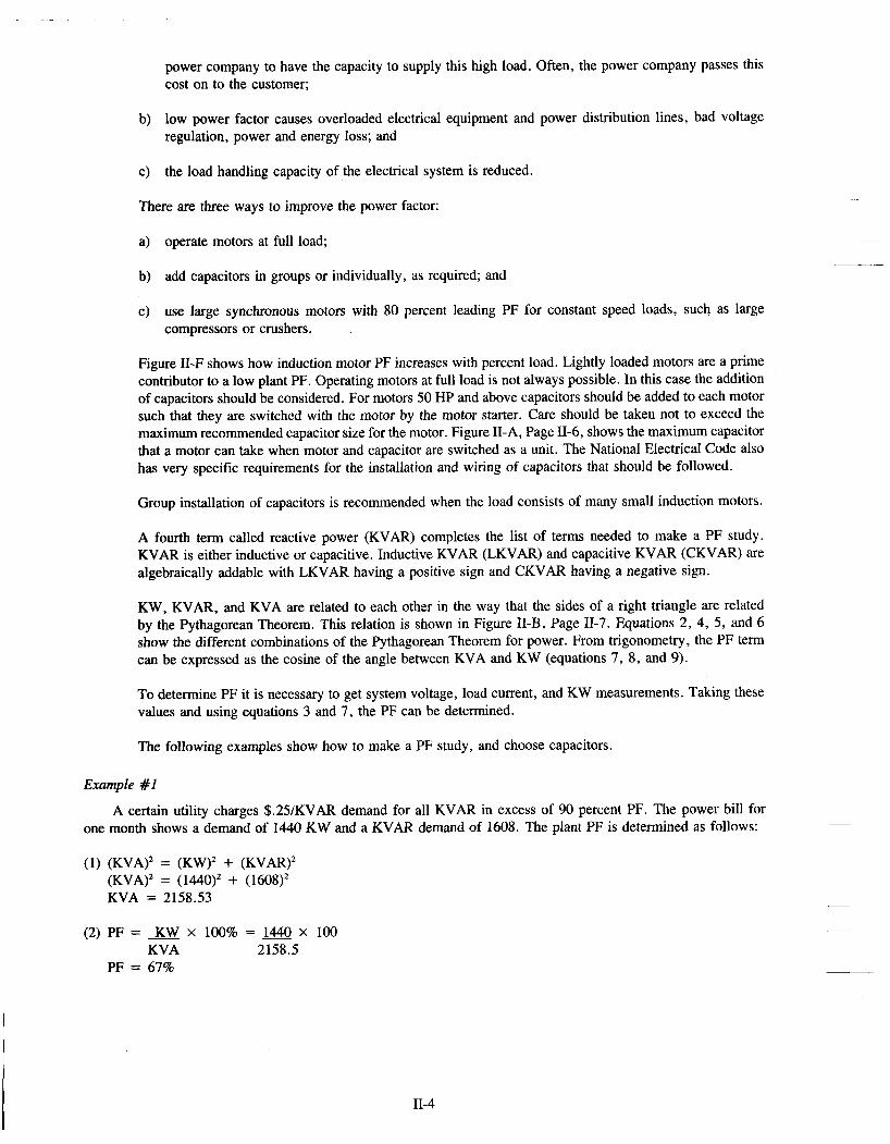
power company to have the capacity to supply this high load. Often, the power company passes this cost on to the customer;

b) low power factor causes overloaded electrical equipment and power distribution lines, bad voltage regulation, power and energy loss; and

c) the load handling capacity of the electrical system is reduced.

There are three ways to improve the power factor:

a) operate motors at full load;

b) add capacitors in groups or individually, as required; and

c) use large synchronous motors with 80 percent leading PF for constant speed loads, such as large compressors or crushers.

Figure 11-F shows how induction motor PF increases with percent load. Lightly loaded motors are a prime contributor to a low plant PF. Operating motors at full load is not always possible. In this case the addition of capacitors should be considered. For motors 50 HP and above capacitors should be added to each motor such that they are switched with the motor by the motor starter. Care should be taken not to exceed the maximum recommended capacitor size for the motor. Figure 11-A, Page 11-6, shows the maximum capacitor that a motor can take when motor and capacitor are switched as a unit. The National Electrical Code also has very specific requirements for the installation and wiring of capacitors that should be followed.

Group installation of capacitors is recommended when the load consists of many small induction motors.

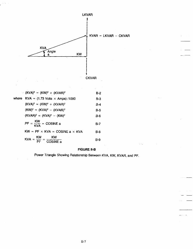
A fourth term called reactive power (KVAR) completes the list of terms needed to make a PF study. KVAR is either inductive or capacitive. Inductive KVAR (LKVAR) and capacitive KVAR (CKVAR) are algebraically addable with LKVAR having a positive sign and CKVAR having a negative sign.

KW, KVAR, and KVA are related to each other in the way that the sides of a right triangle are related by the Pythagorean Theorem. This relation is shown in Figure 11-B, Page 11-7. Equations 2, 4, 5, and 6 show the different combinations of the Pythagorean Theorem for power. From trigonometry, the PF term can be expressed as the cosine of the angle between KVA and KW (equations 7, 8, and 9).

To determine PF it is necessary to get system voltage, load current, and KW measurements. Taking these values and using equations 3 and 7, the PF can be determined.

The following examples show how to make a PF study, and choose capacitors.

Example #1

one month shows a demand of 1440 KW and a KVAR demand of 1608. The plant PF is determined as follows: A certain utility charges $.25/KVAR demand for all W A R in excess of 90 percent PF. The power bill for

(1) (KVA)’ = (KW)’ + (KVAR)’ (KVA)’ = (1440)’ + (1608)2 KVA = 2158.53

(2) PF = KW X 100% = 1440 X 100 KVA 2158.5

PF = 67%

11-4

At 90 percent PF the allowable KVAR is next determined:

(3) @ 90% PF KVA = KW = 1440 = 1600 PF .90

(4) (KVAR)2 = (KVA)’ - (KW)’ (KVAR)’ = (1600)’ - (1440)’

Allowable KVAR = 697.42

(5) Excess KVAR = 1608-698 = 916 KVAR

By adding 916 KVAR in capacitors to the plant electrical system this penalty can be eliminated.

Example # 2

It is desired to determine the plant PF and correct it if necessary to 90 percent. A plant served on a 2300 volt line from the utility has a load of 850 amperes and KW demand of 2500 KW.

First calculate existing plant PF and KVAR:

(1) KVAl = (1.73 Volts X Amps) 110oO KVAl (1.73 x 2300 x 850) /lo00 KVAl = 3382.2

(2) PFl = KW X 100% = 2500 X 100% KVA 3382.2

PF1 = 73.9%

(3) (KVARl)’ = (KVA)2 - (KW)’ (KVAR1)2 = (3382.15)’ - (2500)2 KVARl = 2277

At 90 percent PF, calculate KVAR2:

(4) KVA2 = KW = 2500 = 2777.78 0.90 0.90

(5) (KVAR2)’ = (KVA2)2 - (KW)‘ = (2777.78)’ - (2500)’

KVAR2 = 1210

(6) CKVAR = KVARl - KVAR2 CKVAR = 2277- 1 2 10 KVAR = 1066

By adding 1066 CKVAR in capacitors the plant PF will be increased from 73.9 percent to 90 percent. Note that the 2500 KW load was used in each calculation.

11-5

NOMINAL MOTOR SPEED IN RPM

1800 1200 900 720 Induction Motor Capacitor Capacitor Capacitor Capacitor Horsepower Rating Rating Rating Rating Rating KVAR KVAR KVAR KVAR 3 1.5 1.5 2 2.5 5 2 2 3 4 7.5 2.5 3 4 5.5 10 3 3.5 5 6.5 15 4 5 6.5 8 20 5 6.5 7.5 9 25 6 7.5 9 1 1 30 7 9 10 12 40 9 1 1 12 15 50 1 1 13 15 19 60 14 15 18 22 75 16 18 21 26

100 125 150 200 250 300 350 400 450 500

21 26 30 37.5 45 52.5 60 65 67.5 72.5

25 30 35 42.5 52.5 60 67.5 75 80 82.5

27 32.5 37.5 47.5 57.5 65 75 85 92.5 97.5

FIGURE Il-A*

Maximum Capacitor Rating When Motor and Capacitor are Switched As a Unit.

*“A Guide To Power Factor Correction For the Plant Engineer” Sprague Electric Company, North Adams, Mass., 1962

32.5 40 47.5 60 70 80

95 100 107.5

87.5

11-6

LKVAR

f I I !

1 I I I I

i CKVAR

(KVA)' = (KW)' + (KVAR)' 8-2

where KVA = (1.73 Volts x Amps) /lo00 8-3 8-4

8-5

8-6

(KVA)' = (KW)' + (KVAR)'

(KW)' = (KVA)' - (KVAR)'

(KVAR)' = (KVA)' - (KW)'

p F = - - KW - COSINE^ KVA 8-7

KW = PF x KVA = COSlNEa x KVA 8-8

KW KW KVA = p~ = COSINE a B-9

FIGURE ll-B

Power Triangle Showing Relationship Between KVA, KW, KVAR, and PF.

II-7

Function of Capacitors The power used by industrial plants has two components:

1. Real power which produces work. 2. Reactive power needed to generate magnetic fields required for operation of inductive electrical equipment. No useful work is performed.

Because of the second component, sometimes called “wattless power,” inductive electrical equipment such as motors and transformers must take from the power distribution system more current than is necessary to do the work involved.

The ratio of working current to total current is called the “power factor. ” The function of power factor correction capacitors is to increase the power factor by supplying the “wattless power” when installed at or near inductive electrical equipment.

Fig. 1 REAL POWFR

U I - MOTOR REACTIVE

POWER GENERATOR

Figure 1 shows an induction motor operating under partially loaded conditions without power factor correction. Here the feeder line must supply BOTH magnetizing (reactive) and useful currents.

MOTOR ’ /I I bEACTIVE CDE POWER

CAPACITORS

Figure 2 shows the result of installing a capacitor near the same motor to supply the magnetizing current required to operate it. The total current requirement has been reduced to the value of the useful current only, thus either reducing power cost or permitting the use of more electrical equipment on the same circuit.

Equipment Causing Poor Power Factor A great deal of equipment utilized by modern industry causes poor plant power factor. One of the worst

offenders is the lightly loaded induction motor. Examples of this type of equipment, and their approximate power factors follow:

80 percent power factor or better: Air conditioners (correctly sized), pumps, centerless grinders, cold headers, upsetters, fans or blowers. 60 to 80 percent power factor: Induction furnaces, standard stamping machines, and weaving machines. 60 percent power factor and below: Single-stroke presses, automated machine tools, finish grinders, welders. When the above equipment functions within a plant, savings can be achieved by utilizing industrial capacitors.

How Capacitors Save Money Capacitors lower electrical costs two ways:

In many areas the electrical rate includes a penalty charge for low power factor. Installation of power capacitors on the plant distribution system within the plant makes it unnecessary for the utility to supply the wattless or the non-working power required by the inductive electrical equipment connected to it. Savings the utility realizes in reduced generation, transmission, and distribution costs are passed on to the plant in the form of lower electrical bills.

The second saving possible through the use of power factor correction capacitors is in the form of increased KVA capacity of the electrical distribution system. Installation of capacitors to furnish the non-productive current requirements of the plant makes it possible to increase the plant connected load as much as 20 percent, without a corresponding increase in size of the transformers, conductors and protective devices making up the distribution system that services the load.

11-8

Benefits of Power Factor Improvement

POWER FACTOR

REAL POWER REACTIVE POWER

TOTAL POWER

Power factor (PF) is the ratio of useful current to total current. It also is the ratio of useful power expressed in kilowatts (KW) to total power expressed in kilovolt-amperes (KVA). Power factor usually is expressed as a decimal or as a percentage.

60% 70% 80% 90% 100% 600 KW 600 KW 600 KW 600 KW 600 KW 800 KVAR 612 KVAR 450 KVAR 291 KVAR 0 KVAR

1000 KVA 857 KVA 750 KVA 667 KVA 600 KVA

Useful Power 60 KW Total Power 100 KVA = .60 = 60% - PF = -

60% 360 KW

The significant effect of improving the power factor of a circuit is to reduce the current flowing through that circuit, which in tum results in the following benefits:

70% 80% 90% 100% 420 KW 480 KW 540 KW 600 KW

Benefit No. 1

480 KVAR

600 KVA

Less Total Plant KVA for the Same KW Working Power

Dollar savings are very significant in areas where utility billing is affected by KVA usage.

428 KVAR 360 KVAR 262 KVAR 0 KVAR 600 KVA 600 KVA 600 KVA 600 KVA

100

Percent Speed

80

Benefit No. 2

' I .

/%Load Speed ' I

More KW Working Power for the Same KVA Demand

Released system capacity allows for additional motors, lighting, etc. to be added without overloading existing distribution equipment.

Example: 600 KVA demand vs available KW

POWER FACTOR

REAL POWER REACTIVE POWER

TOTAL POWER

, I

Benefit No. 3

Improved Voltage Regulation Due to Reduced Line Voltage Drop

This benefit will result in more performance of motors and other electrical equipment,

Example: Fig. 3 depicts what happens to the full load speed and starting torque of a motor at various levels of rated voltage.

11-9

Percent Torque and

Full Load Current

160

140

120

100

80

60

40

20 60 70 80 90 100 110 120

Percent Rated Voltage

Benefit No. 4

Reduction in Size of Transformers, Cables and Switchgear in New Installations-Thus Less Investment

Example: Fig. 4 represents the increasing size of conductors required to carry the same 100 KW at various power factors.

KVA-100 KVA-111 KVA-125 KVA.141 KVA-167 P.F.-100% P.F.-90% P.F.-80°/o P.F.-70% P.F.-60°/o

Benefit No. 5

Reduced Power Losses in Distribution Systems Since These Losses are Proportional to the Square of the Current

Since the losses are proportionate to the square of the current, the following formula applies:

original P.F. ( new P.F. )* % reduction of power losses = 100 - 100

Example: Improve power factor from 65 percent to 90 percent.

Reduction of power losses = 100 - 100 (2)’ = 48%

Facts and Formulas

(motor input) KW

1. P.F. = COS^= - KVA

hp x .746 2. KW (motor input) =

(KVA)Z - (KVAR)* KVAR

KW = KVA X P.F. = - - TAN 0-

11-10

V 3 X V X I 3. KVA = (three phase)

KW KVAR (KW)’ - (KVAR)’ KVA = - = - = .\/

P.F. sme V X I

4. KVA = - 103

(single phase)

5 . Motor KVA (approx.) = Motor hp (@ full load)

KVA X lo2 (three phase)

*V 6. I =

KVA x 103 7. I = (single phase) V

8. IC = (27~ f) CV X (single phase)

KVAR x 103 V 3 V

(three phase) 9. IC =

10. I C = KVAR (single phase) - - KVAR = KVA SIN e KW TAN e =V(KVAY - (KWY

27~ fC (KV)’ 103

1 1 . KVAR =

KVAR x 103 (2n f ) (Kv)2

12. c =

1 O6 (27F f) x c

lo6 (27F f) c

13. C =

14. XC = -

where K = 1000 W = watts v = volts A = amperes hp = horsepower I = line current (amperes) IC = capacitor current (amperes) C = capacitance (microfarads) f = frequency

- Improved voltage @ transformer due to capacitor addition: KVAR of capacitors X % reactance of transformer

KVA of transformer % voltage rise =

Note: system reactance should be added to the transformer reactance if available.

- Reduced power losses in the distribution system due to capacitor addition:

Y original power factor ( improved power factor % reduction of losses = 100 - 100

- Reduced KVAR when operating 60 Hz unit @ 50 HZ:

Actual KVAR = rated KVAR - = .83 rated KVAR (3 - Reduced KVAR when operating @ below rated voltage:

operating voltage rated voltage

Actual KVAR = rated KVAR

i.e., 240 V @ 208 = .751 rated KVAR

11-1 1

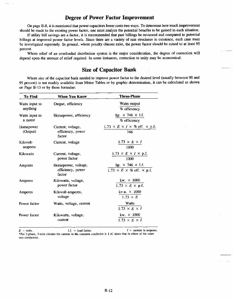
Degree of Power Factor Improvement On page 11-8, it is mentioned that power capacitors lower costs two ways. To determine how much improvement

should be made to the existing power factor, one must analyze the potential benefits to be gained in each situation. If utility bill savings are a factor, it is recommended that past billings be reviewed and compared to potential

billings at improved power factor levels. Since there are a variety of rate structures in existence, each case must be investigated separately. In general, where penalty clauses exist, the power factor should be raised to at least 95 percent.

Where relief of an overloaded distribution system is the major consideration, the degree of correction will depend upon the amount of relief required. In some instances, correction to unity may be economical.

Size of Capacitor Bank Where size of the capacitor bank needed to improve power factor to the desired level (usually between 90 and

95 percent) is not readily available from Motor Tables or by graphic determination, it can be calculated as shown on Page 11- 13 or by these formulae:

To Find When You Know Three-phase

Watts input to Output, efficiency anything

Watts output % efficiency

Watts input to Horsepower, efficiency hp. X 746 X 1.f. a motor % efficiency

Horsepower Current, voltage, (Output) efficiency, power 746

1.73 X E X I x % eff. X p.f.

factor Kilovolt- Current, voltage

Kilowatts Current, voltage,

amperes

power factor

1.73 X E X I 1000

1.73 X E X I X p.f. 1000

Amperes Horsepower, voltage, hp. X 746 X 1.f. efficiency, power factor

1.73 x E x % eff. X p.f.

Amperes Kilowatts, voltage,

Amperes Kilovolt-amperes,

Power factor Watts, voltage, current

power factor

voltage

Power factor Kilowatts, voltage, current

kw. x 1000 1.73 X E X p.f.

kv-a. x lo00 1.73 X E

Watts 1.73 x E x I kw. x 1000

1.73 X E X I ~~ ~

E = volts. *For 2-phase, 3-wire circuits the current in the common conductor is 1.41 times that in either of the other two conductors.

1.f. = load factor. I = current in amperes.

11-12

Determining Your Capacitor Requirements The total KVAR rating of capacitors required to improve a plant power factor to any desired value may be calculated very easily by using the several basic formulas below, and by applying the appropriate multiplier selected from Table 1.

KW-ACTUAL or REAL POWER ESSENTIALLY CONSTANT FOR SAME LOAD

Formulae:

1.

2.

3.

KW or KW = KVA X PF or KVA = - KW

PF PF = -

KVA

Capacitor KVAR = KW X Table I Multiplier

* (amps) x v (volts) or I (amps) = KVA X 1000 KVA (3 phase) = 1.73 X -

1000 1.73 X V (volts)

Examples:

1. A plant with a metered demand of 196 KW is operating at a 52 percent power factor. What capacitor KVAR is required to correct the present power factor to 95 percent?

a. From Table 1, multiplier to improve PF from 52% to 95% is 1.314 b. Capacitor KVAR = KW X Table 1 multiplier = 196 X 1.314 = 257.5, say 260 KVAR.

2. A plant load of 425 KW has a total power requirement of 670 KVA. What size capacitor is required to improve the present power factor to 90 percent?

KW 425 KVA 670

a. Present PF = - = - - - .634 = 63.4%, say 63%

b. From Table 1, multiplier to improve PF from 63% to 90% is .749 c. Capacitor KVAR = KW X Table 1 multiplier = 425 X .749 = 318, say 320 KVAR.

3. A plant operating from a 480 volt system has a metered demand of 258 KW. The line current read by a clip- on ammeter is 420 amperes. What amount of capacitors are required to correct the present power factor to 90 percent?

a.

b.

C. d.

X V = 1.73 X - 420 x 480 = 349 KVA KVA = 1.73 X - I 1000 1000

KW 258 KVA 349

Present PF = - = - - - 73.9, say 74%

From Table 1, multiplier to improve PF from 74% to 90% is .425 Capacitor KVAR = KW X Table 1 multiplier = 258 X .425 = 109.6, say 110 KVAR.

11- 13

Table 1 -KW Multipliers for Determining Capacitor Kilovars

94

1369

1 324 1280 1237 1 196 1 156

1 117 1079 1 042 1006 1970

1936 I903 3870 1838 I806

1775 1745 1715 1686 1657

1629 1601 1573 1546 3519

0 492 D 466 0 439 0413 0 387

0 361 0 335 0 309 0283 0 257

0 230 0 204 0 177 0 149 0 121

0093 0063 0032 0000

Desired Power Factor In Percentage

95 96

1403 1440

1 358 1 395 1314 1351 1271 1308 1230 1267 1190 1227

1 151 1 188 1 113 1 150 1 076 1 113 1040 1077 1004 1041

0970 1007 0937 0 974 0 904 0 941 0 872 0 909 0 840 0877

0 809 0 846 0 779 0816 0 749 0 786 0 720 0 757 0 691 0 728

0 663 0 700 0 635 0672 0 607 0 644 0 580 0617 0553 0590

0 526 0 563 0 500 0 537 0 473 0 510 0447 0484 0 421 0458

0 395 0 432 0 369 0 406 0 343 0 380 0317 0354 0 291 0 328

0 264 0 301 0 238 0 275 0211 0248 0 183 0 220 0 155 0 192

0 127 0 164 0097 0 134 0 066 0 103 0 034 0 071 0 000 0 037

-

- 50

51 52 53 54 55

56 57 58 59 60

61 62 63 64 65

66 67 68 69 70

71 12 73 74 75

76 17 18 79 BO

81 82 83 04 85

86 07 I8 )9 30

Q1 82 83 84 15

86 I7 18 I9

-

80

0 982

0 937 0 893 0 850 0 809 0 769

0 730 0 692 0 655 0 619 0 583

0 549 0 516 0 483 0 451 0 419

0 388 0 358 0 328 0 299 0 270

0 242 0 214 0 186 0 159 0 132

0 105 0 079 0 052 0 026 0 000

- 81

008

I962 I919 I876 835

1795

1756 I718 1681 645 609

575 542 509 474 445

414 384 354 325 296

268 240 212 185 158

131 105 078 052 026

000

- -

82 - I 034

3 989 1945 1902 1861 1821

I782 1744 1707 1 671 1635

1601 I 568 1535 1503 1471

I440 1 410 I 380 1 351 ) 322

1 294 1 266 1238 1 211 1184

1157 1131 1104 1078 1052

1026 I 000

- 83 -

I 060

I 015 1971 1928 1887 1847

1 808 1770 1733 1 697 1661

I627 I 594 I561 I529 I497

I466 I436 I 406 I 3 7 7 I348

I320 I292 I264 I237 I210

1183 1157 1130 1104 1078

052 1 026 1000

- 84 -

I 086

I041 I997 ) 954 1 913 I873

I834 I 796 I759 I723 I687

I653 I620 I587 I555 I523

I492 I462 1432 1403 I374

I346 1318 1290 I263 I236

I209 I183 I156 I130 I104

IO78 I052 I026 I 000

- 85 - 112

067 023

I980 I939 I 899

I 860 I822 I785 1749 I 713

679 646 613 581 549

518 488 458 429 400

372 344 316 289 262

I235 I 209 I182 1156 I130

1104 1078 I052 I026 I 000

- 86 -

1 139

1 094 1 050 1 GQ? 9 966 1926

3 887 1849 1812 1 776 1740

1 706 1 673 1640 1 608 1576

1545 1 515 1485 1 456 1427

1 399 ) 371 1343 1316 1289

1262 1236 1209 3 183 3 157

3 131 1 105 3 079 3 053 D 027

0 000

81 - 1 165

1120 1 076 1 033 0 992 0 952

0 913 0 875 0 838 0 802 0 766

0 732 0 699 0 666 0 634 0 602

0 571 0 541 0 511 0 482 0 453

0 425 0 397 0 369 0 342 0 315

0 288 0 262 0 235 0 209 0 183

0 157 0 131 0 105 0 079 0 053

0 026 0 000

88 - 1 192

1 147 1103 1 060 1019 0 979

0 940 0 902 0 865 0 829 0 793

D 759 0 725 0 693 0 661 0 629

0 598 0 568 0 538 0 509 0 480

0 452 0 424 0 396 0 369 0 342

0 315 0 289 0 262 0 236 0 210

0 184 0 158 0 132 0 106 0 080

0 053 0 027 0000

89 - 1 220

1 175 1131 1 088 1047 1007

0 968 0 930 0 893 3 857 3 821

1787 3 754 3 721 1689 3 657

I 626 I 596 1566 3537 1508

1480 1452 1424 1397 1370

0 343 0 317 0 290 0 264 0 238

0 212 0 186 0 160 0 134 0 108

0 081 0 055 0 028 0 000

- 90

1 248

1 203 1 159 1116 I 075 I 035

9 9% 3 958 1921 1885 1849

1 815 1782 1749 1717 1 685

1654 1 624 I 594 1565 1 536

1 508 1480 1452 1425 1398

1 371 1 345 3 318 D 292 3 266

3 240 1214 0 188 3 162 0 136

0 109 0 083 0 056 0 028 0 ooc

-

-

91

1 276

1231 1 187 1144 1 103 1 063

1 024 0 986 0 949 0 913 0 877

0 843 0 810 0 777 0 745 0 713

0 682 0 652 0 622 0 593 0 564

0 536 0 508 0 480 0 453 0 426

0 399 0 373 0 346 0 320 0 294

0 268 0 242 0 216 0 190 0 164

0 137 0 111 0 084 0 056 0 028

0 000

-

-

- 92

1306

1261 1217 1 174 1 133 1 093

1 054 1016 0 979 0 943 0 907

0 873 0 840 0 807 0 775 0 743

0 712 0 682 0 652 0 623 0 594

0 566 0 538 0 510 0 483 0 456

0 429 0 403 0 376 0 350 D 324

0 298 0 272 0 246 0 220 0 194

0 167 0 141 0 114 0 086 0 058

0 030 0 000

- -

93

1337

1 292 1248 1 205 1 164 1124

1085 1047 1010 D 974 0 938

3 904 D 871 D 838 3 806 0 774

3 743 D 713 3 683 D 654 D 625

D 597 0 569 3 541 D 514 3 487

0 460 0 434 0 407 0 381 0 355

0 329 0 303 0 277 0 251 0 225

0 198 0 172 0 145 0 117 0 089

0 061 0 031 0 000

-

- il

- 91 -

1481

1 436 1 392 1 349 1 308 1 268

1 229 1 191 1 154 I 118 1 092

1 048 1015 0 982 0 950 0 918

0 887 0 857 0 827 n 798 0 769

0 741 0 713 0 685 0 658 0 631

0 604 0 578 0 551 0 525 0 499

0 473 0 447 0 421 0 395 0 369

0 342 0 316 0 289 0 261 0 233

0 205 0 175 0 144 0 112 0 079

0 041 OOOC

-

- 98

1 529

1 484 1 440 1 397 1 356 1316

1277 1 239 1 202 1166 1 130

1 096 1 063 1 030 1998 3 966

3 935 D 905 D 875 3 846 3 817

3 789 3 761 3 733 3 706 D 679

0 652 0 626 0 599 0 573 0 547

0 521 0 495 0 469 0 443 0 417

D 390 0 364 0 33i 0 306 0 281

0 252 0 22: 0 192 0 16( 0 121

0 08' 0 04 0 00

-

-

- 99

1 589

1 544 1 500 1457 1416 1 376

1 337 1 299 1 262 1 226 1190

I156 I123 I 090 I 068 I 026

1995 1965 1935 I 906 1877

1849 182 t I 793 1766 I 739

3 712 3 686 1 659 I 633 D 609

D 581 3 555 D 529 D 503 0 477

0 450 0 424 0 391 0 369 0 341

0 313 0 283 0 252 0 22c 0 18€

0 14' 0 101 0 061 0 WI

-

-

- 1 0 -

1 732

1 M)7 1 643 1 600 1 559 1519

1480 1442 1 405 1 369 1 333

1 299 1 266 1233 1201 1 169

1 138 1 108 1078 1049 1 020

0 992 0 964 0 936 0 909 0 882

0 855 0 829 0 802 0 776 0 750

0 724 0 698 0 672 0 646 0 620

0 593 0 567 0 540 0 512 0 484

0 456 0 426 0 395 0 363 0 329

0 29; 0 251 0 20: 0 14: 0 00(

Example Total KW input 01 load lrom wattmeter reading 100 KW at a power laclor of 60% The leading reactive KVAR necessary l o raise the power laclor 10 90% is l w n d by multiplying Me 100 KW by the factor found in the table which IS 849 Then 100 KW x 0 849 = 84 9 KVAR Use 85 KVAR

4) Instrumentation-The installation of measuring instruments helps in the effort to operate at optimum production and energy usage.

a> Ammeters are the easiest way to measure power usage. The disadvantage of an ammeter is that it does not take into account load power factor. A load with relatively high current, but with low power factor is doing less work (production) than a load with that same current and high power factor. For this reason wattmeters are best for measuring work and loading.

11-14

b) Portable recording wuttmeters are useful when a power and energy study is to be made. This instrument, which can be temporarily installed anywhere in a power system, can be used to identify a machine that is an inefficient user of power or has an excessive KW demand.

c) Utilities use integrating watthour demand meters. This instrument continuously measures energy (KWH), and average power demand (KW) over an interval of time (15 minutes or 30 minutes). At the end of the time interval, the demand counter resets to zero and starts over. The single highest KW demand in a billing period is taken by the utility as the actual demand for that billing period. Depending on the rate schedule, this actual demand figures into the billing demand.

A plant can extend the application of this type instrument into the electrical load centers within a plant. This will give area metering and show exactly where demand and energy is used. If synchronized with the utility, plant demand and energy usage can be correlated with the utility meter. This will aid in identifying ways for off-peak scheduling of production. Figure II-C is a schematic diagram of a recording WHDM installation that would cost about $1 ,OOO.

Incoming 3-Phase Power

Voltage Transformers KW Demand Pulses

1 -phase 120 VAC For Chart Power

r /

Circuit Breaker

WattHour Meter Circulator Chart Equipped with KW Demand Totalizer

(General Electric G-9) KW Demand Contact Device

Current Transformers To Load

Figure 11-C

Typical KW Demand Instrument

Recent developments in electronic technology have made available versatile watthour demand instruments that not only monitor power and energy but control it through the use of set points and alarms. These instruments have readouts that show accumulated KWH and KW demand. When KWH or KW reaches the set point value, an alarm, or contact will operate providing a means of control.

The next step in these electronic instruments is the demand controller. Demand controllers are capable of monitoring plant KW and KWH and turning on or off, in any sequence, literally dozens of loads. For further data on demand and KW control, see section 11-G, page 11-31.

The most important consideration in applying a demand controller is to determine just how much load can be turned on and off. In a crushed stone plant quarry, pumps, air compressors, shop and office loads are the most likely candidates.

d) The best measure of plant electrical energy efficiency is energy use per ton of production, KWH/Ton.

11- 15

The lower this number, the better the energy efficiency. The easiest way to get this number is to divide monthly power usage by monthly production. When compared to an average figure based on a year or more of record keeping, a good idea of how energy efficient a plant has been operating can be determined.

Table II-D, which follows, lists several ways to maintain machine operating efficiency. e)

TABLE II-D A. Fans

1. 2. Keep fan blades clean. 3. 4.

5. 6.

Check for excessive noise and vibration. Determine cause and correct as necessary.

Inspect and lubricate bearings regularly. Inspect drive belts. Adjust or replace as necessary to ensure proper operation. Proper tensioning of belts is critical. Inspect inlet and discharge screens on fans. They should be kept free of dirt and debris at all times. Inspect fans for normal operation.

B. Pumps 1 .

2.

Check for packing wear, which can cause excessive leakage. Repack to avoid excessive water wastage and shaft erosion. Inspect bearings and drive belts for wear and binding. Adjust, repair or replace as necessary.

C. Motors 1. 2. 3 . Keep motors clean. 4. Eliminate excessive vibrations. 5.

Check alignment of motor to equipment drive. Align and tighten as necessary. Check for loose connections and bad contacts on a regular basis. Correct as necessary.

Lubricate motor and drive bearings on a regular basis. This will help reduce friction and excessive torque, which can result in overheating and power losses. (For detail grease applications see Section II-F, p. 11-42)

6. Replace worn bearings. 7. 8.

Tighten belts and pulleys to eliminate excessive losses. Check for overheating. It could be an indication of a functional problem or lack of adequate ventilation.

D. Conveyors 1. Lubricate idlers. A stuck idler can cost $100/year in energy usage.

5 . Electric Motor Design

When selecting an electric motor for a particular application the first thing most people think of is horsepower, followed by speed and voltage. It is true that these three characteristics are of primary importance, but the motor selection process should not stop here. There are several other characteristics of equal and perhaps more importance. The following is a list of these other characteristics that should be considered.

a) Insulation Class b) Ambient Temperature Rating c) Temperature Rise d) Service Factor e) NEMA Design Type (Torque) f) Power Factor and Efficiency g) System Voltage and Frequency Variation

Items “a” through “d” are all related to motor heating, which is lost energy.

II- 16

a) Insulation Class Motor insulation materials are divided into four classes, which correspond to the maximum temperature the insulation can withstand before it begins to degrade. The four classes are:

Class Max Temperature A 105 C (221F) B 130 C (266F) F 155 C (311F) H 180 C (356F)

At present most motors have Class B insulation with a trend toward Class F. With the Class F insulation, a motor can take more overloads for longer periods of time without reducing life expectancy, which is about 20 years.

b) Ambient Temperature40 C (104F)

A motor will be at the same temperature, before running, as the surrounding air, which is the ambient temperature. All motor ratings are at ambient temperature. NEMA has standardized this value at 40C. Special motors may have 65C or 90C ambient ratings.

c) Temperature Rise

This is the temperature increase that a motor can withstand for short periods of time and still maintain its rated values. For each class of winding insulation these temperature rises are as follows:

(1) (2) (3) (4) (5) (6) Max. Rated Hot Spot Safety

Class Temp. Temp. Rise Ambient Allowable Factor A 105C (221F) 40C (72F) 40C (104F) 15C (27F) 1OC (18F) B 13OC (266F) 60C (1 08F) 40C (104F) 20C (36F) 1OC (18F) F 155C (311F) 75C (1 35F) 40C (104F) 25C (45F) 15C (27F) H 18OC (356F) 90C (162F) 40C (104F) 30C (54F) 20C (36F)

Notice that columns 3,4,5, and 6 add to give column 2, insulation class maximum temperature. Column 5 is a factor manufacturers use to allow for differences between the temperature at the point of measurement and a theoretical hottest point in the winding. Column 6 is a factor that manufacturers use to allow some overheating above rated temperature rise.

It should be pointed out that if a motor is operated above a 40C ambient, it will not have its rated temperature rise. In general, for each degree above ambient, one degree must be subtracted from the rated temperature rise.

d. Service Factor

General purpose motors of 200 HP or less are given a “service factor.” Service factor is a multiplier which, applied at rated voltage, indicates a permissible loading which may be carried continuously under the conditions specified for that service factor. This is done by providing for a higher temperature rise. However, if a motor is operated at service factor load, the insulation life of the motor may be reduced by more than half. The table below compares the temperature rise of motors with a 1.0 SF with motors having a 1.15 SF.

Class B Class F 1.15 SF 90C 115C 1.0 SF 60C 75c

11- 17

In summarizing the importance of insulation, temperature rise, and service factor we should look at cost and enclosure. First, comparative costs of typical motors are shown below.

HP V RPM Enel. SF Insulation List Cost 25 460 1800 DP * 1.15 B $1226.00 25 460 1800 TEFC ** 1 .oo B $1230.00 25 460 1800 TEFCXT*** 1 .o F $1542.00 25 460 1800 TEFC XT 1.15 F $1542.00

* OpenDripProof

*** Heavy Duty Motor ** Totally Enclosed Fan Cooled

From this it is seen that the drip proof motor will be the most motor for the least cost, provided that the environment is acceptable.

e) NEMA Design Type

Second to horsepower, this may be the most important characteristic that a motor has. The motor design type describes the motor torque and speed relationship. AC induction motors are divided into four design types, which are:

Design A-Normal starting torque, Normal starting current,

Design B-Normal starting torque, Low starting current,

Design C-High starting torque, Low starting current,

Design D-High slip

Slip is defined as the percent difference between the motor’s synchronous or rated speed and actual speed.

% S = [(Ns - N,) + N,] X 100%

For example, if the synchronous speed of a motor is 1,800 RPM, the actual speed, depending on the driven machine load, would be nominally 1,760 RPM and the slip would be:

S = [(1800-1760) + 18001 X 100% = 2.22%.

Slip will vary from 1 or 2 percent at no load to 4 or 5 percent at full load.

The torque a motor develops varies as the speed of the motor. The speed-torque characteristics of the various design type motors are shown in Figure 11-E. The differences in the design types are clearly shown by these curves.

Note from the curves that full load torque is developed at a speed less than synchronous speed. If the load torque is less than full load, this actual speed will increase some, or if the load torque is greater than full load, the motor’s actual speed will be slower. If the load torque ever exceeds the motor torque, the motor will stall causing the motor starter overloads to trip. This sometimes happens when conveyors or crushers are overloaded. Ideally a motor should be operated at as near full load as possible to obtain best operating efficiency and power factor.

When a motor operates at low efficiency, the power losses are higher than when the motor operates at high efficiency. These power losses contribute directly to the kilowatt demand and energy usage on the power bill but do not contribute to plant production.

11- 18

Desinn D

0 10 20 30 40 50 60 70 80 90

Percent Synchronous Speed

Slip - 100

- Note: Full Load Torque is determined by

the equation T = F w v ft. Ibs.

Where HP is nameplate horsepower and N is rated speed.

Figure 11-E

Speed Torque Characteristics of NEMA Design A,B,C, and D 3-Phase Induction Motors

Similarly, a motor that operates at low power factor will require more current to develop load horsepower than one that operates at a high power factor. This higher current causes voltage drop in the power lines, and energy losses. Utilities are required to increase the size of their equipment to handle the higher power requirements and often penalize a customer for poor power factor. By operating the motors at high efficiencies and power factors these losses are reduced or eliminated.

Figure 11-G shows a typical load speed-torque curve superimposed on the motor speed-torque curve with machine breakaway, accelerating, and peak running figures shown. Breakaway torque is the torque required to start the shaft turning. Accelerating torque is the torque required to bring the load from standstill to rated speed. Peak torque is the maximum torque that a load will require. Table 11-H lists these torque requirements for machines commonly found in a crushed stone plant.

Table 11-1 shows the PF and efficiency for 3-phase AC induction motors at %, Y4 and full load.

f) Power Factor and EfJiciency

The power factor and efficiency of electric motors vary as the load on the motor. Figure 11-F shows

11-19

how efficiency and power factor vary under various loads. It is emphasized that these curves reflect nominal values. Actual efficiencies and power factors will vary from motor to motor.

100

80

60

40

20

I I I I I I I I I I I I I I I I I I

0 10 20 30 40 50 60 70 80 90 100

Percent Load

FIGURE Il-F

Nominal Efficiency and Power Factor Curve For 3-Phase induction Motor

200 a, 3 e 2 D m 0

-J - 100

I C a,

a, a 2

Breakaway Torque

10 20 30 40 50 60 70 80 90 100

Percent Synchronous Speed

FIGURE Il-G

Typical Load Speed-Torque Curve Superimposed on Design B Motor Speed-Torque Curve.

* Peak running torque usually occurs momentarily while machine operates at full load.

** Accel. Torque = (Motor Torque) - (Load Torque)

11-20

Table II-H LOAD TORQUE REQUIREMENTS OF VARIOUS MACHINES

(In O h of Full Load Torque**)

Breakaway Accelerating Peak Running Machine Torque % Torque % Torque % Agitators (Liquid) Agitators (Slurry) Compressors, Recip

(Start Unloaded) Conveyors-Belt (Loaded) Conveyors-Screw (Loaded) Crus her-G yratory

(Start Unloaded) (Choke Fed)

Crusher-Jaw (Start Unloaded)

Crusher-Hammermill Crusher-Roll

(Choke Fed) Fans-Centrifugal

Ambient-Valve Closed

Hot Gas-Valve Closed Valve Open

Valve Open Pumps-Centrifugal

1 00 1 50

40 110 150

50 100

50 50 50 200

25 25 25 25 40

1 00 100

50 130 100

60 200

100 100 50 200

60 110 60 200 100

100 100

1 00 100 100

300 300

200 150

1 50

50 100 100 175 100

-

“Robert W. Smeaton “Motor Applications and Maintenance Handbook,” McGraw Hill 1969, pp. 1-6 through 1-14. *‘Full Load Torque = (Load HP x 5250) + RPM

Table 11-I*

% EFFICIENCY AND POWER FACTOR FOR 3-PHASE AC INDUCTION MOTOR AT 1/2, 3/4 AND FULL LOAD

112 Load 314 Load Full Load Motor HP PF EFF. PF EFF. PF EFF.

1 75 57 77 69 76 76 3 80 70 82 80 81 84 5 80 76 82 83 82 86 7% 83 77 85 84 85 87 10 83 81 85 86 85 88 15 84 82 86 85 88 87 20 87 82 88 86 87 87 25 87 83 88 86 87.5 87 30 87.5 84 88.5 86 88.5 87 40 87.5 84 89 87 89.5 88 50 87.5 84 89 87 89.5 88 60 88 84 89.5 87 89 88 75 88.5 84 89.5 87 89.5 88 100 89 84 90 88 90.5 88 125 90 84 90.5 88 91 89 150 90 84 91.5 88 92 89 200 90 85 91.5 89 92 90 250 91 84 92.5 89 93 90 300 92 84 93.5 89 94 90 ‘Croft, Carr, and Watt, “American Electricians Handbook,” 9th Edition, McGraw-Hill, 1970, pp. 7-88.

11-2 1

g) System Voltage and Frequency Variation

System voltage and frequency variations have an effect on how a motor performs. Table II-J shows the effect of high and low voltage and frequency on a motor. Frequency variations usually are not a problem from utility supplied plants, but may be from those plants that get power from a portable engine-generator.

TABLE II-J

Characteristic

EFFECT OF VOLTAGE AND FREQUENCY VARIATION ON INDUCTION MOTOR CHARCTERISTICS

Voltage Frequency 1 1 0% 90% 110% 90%

~~~~~ ~

Torque Speed-Synchronous

Full Load Slip

Eff iciency-I 00% Load 75% Load

Power Factor-I 00% Load 75% Load 50% Load

Current-Start Run

Temp. Rise Overload Capacity

+ 21% - 19% Negligible Effort

- 17% + 23% + .75% - 2%

0 0 - 3% + 1% - 4% + 2% - 5% f 4% + 10% - 10% - 7% + 11% - 3°C + 6°C + 21 Yo - 19%

+ 1% - 1.5%

- 10% + 1 1 Yo

4- 5% - 5% 4- 5% - 5%

Negligible Effect Negligible Effect Negligible Effect Negligible Effect Negligible Effect Negligible Effect

Negligible Effect Negligible Effect Negligible Effect

- 5% + 5%

C. Diesel Equipment

1) Plant Production Facilities

Diesel fuel is the second largest energy source used in the quarrying industry. It can be converted directly to mechanical energy through a diesel engine directly connected to the load or connected by mechanical transmission means such as shafts, V-belts, chains, gears, etc. Or the diesel engine can be used to drive a generator and the electric energy so produced can be conveyed by wire to an electric motor and there converted into mechanical energy.

In either form the use of diesel energy does at the same time provide flexibility and yet is restrictive. Diesel engines can be towed, hauled, or driven to many remote sites where electric distribution systems are not available. In these cases, diesel operated plants lend themselves to being portable. However, once the diesel power is converted to a mechanical or electrical form, it must by nature be adjacent to or at least very close to the load.

When the option of either using electric power furnished from a power company or diesel power or generators is available, the operator is again cautioned to consider all factors, not just the cost of fuel versus the cost of electricity. This is discussed earlier in this section under II-B . The costs will be reviewed later under Section 111.

2 ) Diesel-Powered Mobile Equipment

In most quarries some portion of the handling of feed material in the production line, and again as finished products to stockpile or to the customer, is done in diesel-powered equipment. Shovels and front-end loaders load shot rock from the muckpiles. Trucks carry to the crusher, interplant, and ultimately to stockpiles and customers.

11-22

Operators can take steps to reduce fuel consumption without compromising performance. These steps include:

a) Vehicle Selection

1) Give serious time and thought to matching vehicle selection to your type of operations. Recognize that larger vehicles use less fuel per ton of payload. Selection of larger equipment, however, must take into account other factors such as compatibility with other equipment, plants and shops as well as initial investment.

Quarry size, depth, and method of operation should influence vehicle selection too. If you operate a flat quarry or one with only slight grades, consider hauling with tractor trailer type vehicles. They transport approximately 60 percent more payload per gallon of fuel.

Example:

A comparison was made between a 35 ton rear dump and a 70 ton tractor trailer. Both vehicles had Detroit Diesel 12V71N engines with 55MM, (N) injectors, and were operated under the same conditions on a hard packed surface:

A 35 tod24 cubic yard consumed 5.5 gallons/hour-ll.3 yarddgallon. A 70 ton/40 cubic yard consumed 5.7 gallons/hour- 18.2 yarddgallon.

Approximately a 61 percent greater productivity per gallon of fuel.

2) When selecting haul trucks, scrapers and basically all off-highway vehicles, you should discuss carefully planetary gearing ratios so that the practical, obtainable speeds on your existing haul roads will be done at a lock-up point in the transmission as opposed to a converter mode. The hauling transmission is operating at a 70 percent efficiency factor while in the converter mode, as opposed to an 85 percent plus efficiency factor in the lock-up position.

3) Today the two leading hauling transmission manufacturers are strongly advocating the use of automatic transmissions in smaller tonnage trucks, and in the larger units of approximately 75-125 tons, the electro-hydraulic shift control mechanism (better known as the “Black BOX’ ’). This will take the shifting responsibility away from the operator. Both of these systems will lead to better fuel economy.

b) Maintenance

1) Keep your engine tuned at the recommended time intervals. It is very difficult to determine the exact number of hours an engine should run before a tune-up is required, due to the many variables encountered in the multitude of quarrying operations across North America. One should, however, investigate all power complaints or reports of black smoke. When these two warning signs appear, it is obvious that the engine is beginning to use excessive fuel. The case may not necessarily be one of an expensive engine tune-up, but of a plugged air filter cartridge. Or it can be caused by blockage of the intake plumbing, such as a damaged or misplaced snorkel. Either case would rob the engine of air and cause a low air-to-fuel ratio and hence low power.

Consider using proper Vortex of Donaldson Air Restriction gauges in order to change the air filters of naturally asperated engines at 25 inches of vacuum and turbo-charge engines at 20 inches of vacuum. Too much fuel is wasted in waiting for the red marker to appear in the standard restriction gauge.

Check the date of your engine’s last fuel system calibration (valves and injectors). Also make sure engine performance has not grown significantly due to changes in fuel pump adjustment. Increasing fuel rate (over-fueling) and governor cut-off speed (over-speeding) are inefficient ways to improve performance and may be illegal due to environmental regulations. A 10 percent increase in power gained this way can use 15 percent more fuel.

11-23

2 ) Filter out any water in fuel storage tanks and check tanks for leaks. Water is the greatest enemy of the diesel engine injector system.

Keep fuel tank breathers clean and fuel tanks tightly sealed. Top your tanks at night when your engines are hot in order to leave little room for condensation to gather ovemight.

Change fuel filters at the recommended intervals. These intervals should be determined after consultation with the engine manufacturer and the fuel supplier.

3) A constant study of tire performance pays dividends.

Irregular or early excessive tire wear could be due to frame or wheel misalignment, incorrect inflation or tire mis-match or imbalance. It takes extra power and therefore, extra fuel to wear tires prematurely.

4) In cold climate conditions ensure that engines have proper block and/or oil pan heaters for prompt starting. Electric heaters that are properly sized to the engine (either 1500, 1750, or 2000 watts need only three to four hours to bring an engine up to desired starting temperature (100 F). This is based on 20 F ambient temperature with slight modifications required for colder days.

Since it is not necessary to run heaters all the time, we should consider timers with thermostat relays (for ambient temperature). This will provide early moming start-up and automatic shut-off.

Where electricity is not available, diesel fuel heaters can be used to preheat the cooling system liquid. Cold engines waste fuel.

c) Payload

Obviously, an increase in payload decreases the fuel requirements per ton. For quarry trucks the limitations have always been the carrying capability of the truck bed relative to spillage, particularly when going up ramps. The construction of lower grade ramps permits bigger payloads. A recent development of tailgates for quarry trucks has proven very beneficial in increasing payloads 15 to 20 percent.

For over-the-road trucks the gross load is limited by legal requirements. Care should be exercised here when making the initial purchase. Aluminum bodies, fiberglass cabs, abrasion metal in wear areas only versus heavier bodies, all permit the payload to become a bigger percentage of the allowable gross.

D. Pump and Fan Systems

1) General

Pumps and fans are equipment involved in conveying a liquid or gas from one point to another. Four considerations enter into the design of these systems:

(a) quantity and quality of liquid or gas; (b) distance, both vertical and horizontal; (c) capabilities of the pump or fan; and (d) capacity of the conveying pipe line.

The last three items can be juggled in such a way as to have a real influence on capital outlay, energy consumption and maintenance, and all should be considered.

2) Distance

We repeat here for emphasis the definition of energy as first presented in Section 11-A, the capacity to do work, and work as application of force over a distance. It follows then that a reduction in distance results in a reduction in energy usage. Where possible then, place the fan or pump in such a manner as to have the shortest conveying distance possible.

11-24

When the pumping is addressing the water accumulating from the surface runoff and underground seepage, two possibilities should be recognized. As a quarry is deepened, a new sump and discharge pumping system should be maintained for each lift. In this manner the water accumulating at each level need only be pumped from its level to the surface. The less attractive option is to allow it all to accumulate at the lowest lift and pump the entire quantity the maximum height.

A word of caution, however, is warranted. This is only valid if each level has its own piping system to the surface. A relay system where the lowest pump discharges to an intermediate lift is vulnerable to the very real possibility of seepage occurring back to the bottom level. In this case a portion of the water is recirculating and being pumped multiple times.

3 ) Pump and Fan Design Considerations

Centrifugal fans and centrifugal pumps have the same characteristics. The fan and pump laws we should be concerned with relate to speed changes. A speed change from one RPM to another will affect volume, pressure and horsepower as follows:.

I RPM2 = Volume 2 RPM 1 Volume 1

I1 (RPM 2) = Pressure 2 (RPM 1) Pressure 1

111 (RPM 2) = - HP 2 (RPM 1) HP 1

Thus a 10 percent increase in speed will:

Increase volume 10 percent; Increase pressure 21 percent; and Increase horsepower 33 percent.

A 10 percent decrease in speed will:

Decrease volume 10 percent; Decrease pressure 19 percent; and Decrease horsepower 27 percent.

From these numbers one can see that a small reduction in fan or pump speed can offer a significant reduction in power. Many pumps are direct connected, however, and would have to be equipped with a belt drive to accomplish a speed change. There is one other option short of changing pumps, and that is to install a smaller impeller in the pump. (Those operations with a machine shop might consider turning the existing impeller down on a lathe.) A 10 percent reduction in impeller diameter will:

Reduce volume by 10 percent; Reduce pressure by 19 percent; and Reduce horsepower by 27 percent.

Caution-a 10 percent or larger impeller reduction should be checked with the pump manufacturer. In addition, a loss in pump efficiency occurs when impeller size is reduced within a given casing, reducing power savings below the theoretical calculated values.

To utilize the pump and fan laws to save energy, we must check out fans and pumps to see where they stand. Signs to look for are:

a) A fan damper or slide gate continually closed more than 25 percent.

11-25

b) A pump running against a throttling valve.

c) A pump cycling off and on to maintain a level.

d) Fans or pumps delivering more flow than needed.

FAN SPEED CHANGE

A typical energy waster is a dust collector fan. In many cases, they are installed and the dampers opened up and left. If the fan is oversized, as many are, this not only wastes power but shortens bag life, etc.

Gradually close the damper or slide gate (install a simple slide gate if there is no damper) until you just maintain adequate venting under all conditions. Reopen the damper about five percent and lock in place. Allow for sufficient time to check for variations in operating conditions, temperature, etc. , then evaluate a speed reduction.

Ideally, you would measure the airflow through the fan with a pitot tube, and locate the fan operating point on the fan curve. As a quick altemate, measuring fan motor amps and comparing them to full load amps as given on the motor nameplate will allow you to calculate percent of rated horsepower drawn. Locating this on the fan curve gives you an operating point.

Next, measure the static pressure on the inlet and outlet of the fan. Adding these gives you the static pressure the fan is overcoming.

You now have the CFM and static pressure which the fan must develop and can calculate a new fan speed. For example, take a 50 HP fan running at 1400 RPM. After you have adjusted the damper and determined

the proper setting, you note that the damper is 50 percent open. Measuring the fan amps at this setting, you determine that the motor is running at 40 percent of full load, or drawing .4 X 50 = 20 HP. Measuring the static pressure on the inlet and outlet you obtain -6 inches and + 1 inch, for a total of 7 inches of water column. Using the fan curve, Figure 11-K, you find that the airflow for 20 HP is 8,000 CFM. Also, you note the fan will deliver 14,000 CFM at 7 inches by projecting the 7 inch static pressure point downward.

Next we construct new fan curves at various lower speeds to determine at which speed the fan will deliver 8,000 CFM at 7 inches:

1400 RPM 1200 RPM 1100 RPM

(1) (2) (3) (1) (2) (3) (1) (2) (3) CFM S.P. H.P. CFM S.P. H.P. CFM S.P. H.P.

12,000 9.5 30 10,286 7.0 19.5 9,429 5.9 14.6 10,000 11.5 24.5 8,571 8.5 15.4 7,857 7.1 11.0 8,000 13.0 20.0 5,878 9.6 12.6 6,286 8.0 9.8

Note that the 1200 and 1100 RPM columns are developed by multiplying column (1) by the ratio of the speeds, column (2) by the speed ratio squared, and column (3) by the speed ratio to the third power. Plotting the 1100 RPM speed on the fan curve shows the fan performance at this new speed, developing the required 7 inches static pressure at 8000 CFM, requiring 12 HP instead of 20.

Neglecting motor efficiency changes, this exercise has shown a way to cut back eight horsepower with an

Pump speed changes can be handled in a similar manner to that shown for fans. annual dollar saving of $300 to $600.

4) Pipeline Capacity

Pipeline size and configuration is a large factor in pumping costs. For example, 1000 feet of horizontal 6-inch line handling 1000 GPM of water will require a pump pressure of 27 psi just to overcome pipe friction. An 8-inch line, under the same conditions will require only 7 psi to overcome friction. With a pump efficiency of 70 percent, this translates to an additional 17 HP required to pump through the 6-inch line, due to line size alone. Adding the additional losses due to elbows, valves, and other fittings, this can add up to a considerable difference in operating costs over the life of a pipeline. When installing a new line or replacing an old one, have the engineer calculate the head losses at various sizes of pipe and work out the horsepower difference. A larger line will cost more, but will save power and possibly reduce the cost of pump and motor.

11-26

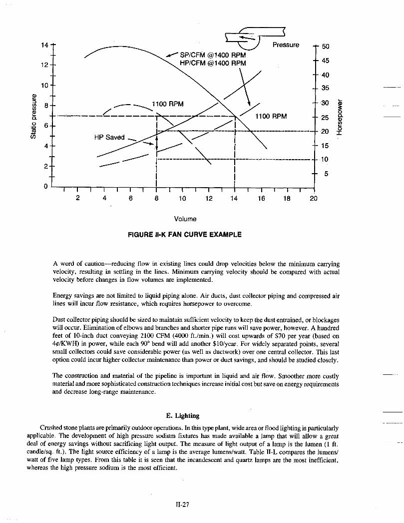
14

12

10 2 v) 2 8-- E 2 6- - G

Q

a

-- 4

2 -- --

0

Volume

-- -- 45

-- 40

-- 35

-- --

-- --

-- .-------------

--

-- 5

--

I I I

I I I I I l l I l l I I I I I I I I

FIGURE Il-K FAN CURVE EXAMPLE

A word of caution-reducing flow in existing lines could drop velocities below the minimum carrying velocity, resulting in settling in the lines. Minimum carrying velocity should be compared with actual velocity before changes in flow volumes are implemented.

Energy savings are not limited to liquid piping alone. Air ducts, dust collector piping and compressed air lines will incur flow resistance, which requires horsepower to overcome.

Dust collector piping should be sized to maintain sufficient velocity to keep the dust entrained, or blockages will occur. Elimination of elbows and branches and shorter pipe runs will save power, however. A hundred feet of 10-inch duct conveying 2100 CFM (4000 ft./min.) will cost upwards of $70 per year (based on 4$/KWH) in power, while each 90" bend will add another $lO/year. For widely separated points, several small collectors could save considerable power (as well as ductwork) over one central collector. This last option could incur higher collector maintenance than power or duct savings, and should be studied closely.

The construction and material of the pipeline is important in liquid and air flow. Smoother more costly material and more sophisticated construction techniques increase initial cost but save on energy requirements and decrease long-range maintenance.

E. Lighting

Crushed stone plants are primarily outdoor operations. In this type plant, wide area or flood lighting is particularly applicable. The development of high pressure sodium fixtures has made available a lamp that will allow a great deal of energy savings without sacrificing light output. The measure of light output of a lamp is the lumen (1 ft. candle/sq. ft.). The light source efficiency of a lamp is the average lumendwatt. Table 11-L compares the lumens/ watt of five lamp types. From this table it is seen that the incandescent and quartz lamps are the most inefficient, whereas the high pressure sodium is the most efficient.

11-27

TABLE II-L

Light Source Efficiency

Lamp Type Incandescent Quartz Mercury Vapor Metal Halide High Pressure Sodium

Example:

Average Lumens Per Watt 22 22 55 90

125

A 400 watt high pressure sodium lamp produces nominally 400W X 125 lumens/watt = 50,000 lumens. At 22 lumendwatt, 2272 watts of incandescent or quartz lighting is required to produce the same light. In other words, it takes 2272 watts + 400 watt = 5.7 times as much power (and energy) of incandescent or quartz lighting to do the same job as a 400 watt high pressure sodium lamp.

Similarly, it would take 2.25 times as much mercury vapor lamp wattage to do the job of the high pressure sodium fixture.

APPROX. IF YOU NOW HAVE TRY THIS MAINTAINED

TYPE OF OR ARE CONSIDERING HPS SYSTEM Yo ENERGY LIGHT APPLICATION: THIS SYSTEM: (LAMP + BALLAST): SAVINGS INCREASE

750R52 Incandescent LU250/DX UP TO 59% + 50% lNDUSTRIAL 1 OOOW PS52 Incandescent LU250 UP TO 70% + 23%

BAY 1000 W Mercury LU400 UP TO 57% + 13% BUILDING 1OOOW Mercury LU400 UP TO 57% + 13% FACADE 400W Mercury LU250 UP TO 33% 4- 33%

1 OOOW Mercury LU400 UP TO 57% 4- 13% AREA 400W Mercury LU200 UP TO 45% 4- 55%

150W PAR Incandescent LU70/DWRFL UP TO 37% + 40% 400W Mercury LU250 UP TO 33% + 93%

175W Mercury LU 100 UP TO 33% + 19% 250W Mercury LU 1 50 UP TO 34% + 47%

1 OOW Mercury LU70 UP TO 24% + 63%

SECURITY 1 OOW Mercurv LU50 UP TO 50% + 13% 1 OOW Mercury LU70/DWMED UP TO 24% EQUAL

175W Mercury LU100 UP TO 33% + 19% 150W Incandescent LU50 UP TO 60% + 53% 150W Incandescent LU70/RFL UP TO 37% + 10% DOCK

WAREHOUSE 400W Mercury AISLES 400W Mercurv

LU250 UP TO 33% + 93% LU250/DX UP TO 33% + 62%

BLDG. ENTRY 150W PAR Incandescent LU35 UP TO 70% + 9% STAIRWELL 150W PAR Incandescent LU7O/DWMED UP TO 37% + 64%

11-28

LAMP EFFICIENCY

$52,004

INCANDES’CENT 17-24

MERCURY

74 100

!32 1 1 I63

FLUORESCENT

’

- $31,374 ’ -

$17,952 $16,480 - - - -

0 10 20 30 40 50 60 70 80 90 100 110 120 130 140 150

Lumens Per Watt (Avg.) Ballast watts not included.

COST COMPARISONS

Example: Annual costs to light a facility of 50,000 square feet to 50 footcandles, (4000 hours pedyear, $.OG/KWH, $5.00 labor/lamp):

1 ooow 1 ooow 400 W High 400W 1 ooow Incand. Deluxe Multi- output Lucalox Lucalox

( V W (LW WM) Mercury Vapor Fluorescent

Furnished By General Electric

11-29

COST OF LIGHT

0 FLOODLlGHT/NlGHT

0 BASED ON 4,000 HOURS PER YEAR

0 $10 LABOR TO REPLACE A LAMP

0 $.07 PER KWH ELECTRICITY RATE

9002 LESS 10% PRICES

Q1500 LU400 LAMPS (240V) $ 22.66 $ 7.66 LABOR 20.00 1.70 ELECTRICITY 420.00 96.00

$466.66 $105.36

ANNUAL SAVINGS PER SOCKET-$361.30


HOW TO CALCULATE ANNUAL ELECTRICITY COST

WATTAGE OF FIXTURE WATTS X HRS. USED/YEAR

EQUALS WATT HRSNEAR t BY 1000 TO EQUAL (KWH)

KILOWATT HRSNEAR MULTIPLY BY RATE CHARGED

PERKWH = $ PER FIXTURE

KWHNR

# OF FIXTURES x ANNUAL COST PER FIXTURE = SYSTEM COST

Note: * There are 8760 hours in one year * $.07 per KWH is the average cost of electricity


F. Grease Application Guide

The grease application guide shown as Exhibit A on the next page will assist the end user in making a preliminary selection. Thickener is given so the user can be aware of the possibility of incompatibility among products and take suitable precautions. Properties are shown for greases made from 10 thickeners, along with remarks and an indication of important uses. Some of the ratings given are subjective and will vary significantly from one supplier to another, but it is believed that user and equipment builder can find a helpful starting point in this table. The greases described are fully formulated products, as found in the marketplace.

The following glossary may be helpful in the application of the guide to specific needs:

1) Dropping point: Grease does not have a sharp melting point. Instead, on heating, it becomes softer until at some point it no longer functions as a thickened lubricant.

2) Water resistance: Deals with the ability of the grease to maintain consistency under water exposure.

3 ) Work stability: The subjection of lubricating grease to any form of agitation or shearing action.

11-30

Oxidation stability: The ability of a grease to hold up under oxidation. Most technologists believe that the only practical measure of service oxidation would be obtained in an actual operating bearing.

Protection against rust: Rusting may be controlled, or even prevented, by incorporation into the lubricant of a suitable rust inhibitor.

Pumpability: Indicates the ease of pumping and dispensing grease and is valuable in estimating the pressure drop in a distribution system, or in determining the optimum pipe diameters for such a system.

Oil separation: Thickener is not soluble in the oil it thickens but must have some attraction for that oil. When more oil is added or thickener decreased, the force between the thickener and oil decreases resulting in some of the oil in a grease being loosely held and easily separated.

Note: Souce material from the National Lubricating Grease Guide.

EXHIBIT “A’

GREASE APPLICATION GUIDE

Calcium- Calcium- Aluminum Calcium Lithium PrOlJeftbS Aluminum Sodium Lithium Comdex Conventional Anhydrous

205-220 275-290 96-104 135-143 200 230

Complex

500 + 260 + 350

Complex

500 + 260 + 350

Polyurea

470 243 350

OrganeClay

500 + 260 + 350

Dropping point (F) 230 Dropping point (C) 110 Maximum usable 175 temperature (F) Maximum usable 79 temperature (C) Water resistance Good to

excellent Work stabili Poor

Oxidation stability Excellent

325-350 163-177 250

350-400 177-204 275

500+ 206 + 350

121 93 110 135 177 177 177 177 177

Poor to fair Good to Excellent excellent Fair to good Good to

excellent Poor to Fair to excellent excellent Poorto Poorto excellent excellent Good to Fair to excellent excellent Poorto Good

Smooth and S m t h and buttery buttery EP grades EP grades available available

good

Good Good to excellent Good to excellent Fair to excellent Good to excellent Fair to good

Fair to excellent Fair to good

Good to excellent Good to excellent Fair to excellent Fair to excellent Good to excellent Good to excellent Smooth and buttely EP grades available

Good to excellent Poor to good Good to excellent Fair to excellent Good to excellent Good to excellent Smooth and buttery EP grades available

Fair to excellent Fair to good Fair Good to

excellent Fair to excellent Poor to excellent Fair to excellent Good to excellent Smooth and buttery EP grades available, reversible The leader

Poor to good Good to excellent Poor to fair

Poor to good Fair to excellent Poor to fair

Good

Protection against rust Good to excellent

Pumpability (in centralized Poor system) Oil separation Good

Poor to excellent Good

Fair to good Smooth to fibrous Adhesive & cohesive

Good to excellent Smooth and buttery EP grades available, reversible Increasing

Good to excellent Smooth and buttery EP and antiwear inherent Declining

Multiservice automotive & industrial

Good to excellent Smooth and buttery

Appearance Smooth

Other properties and dear

Production volume and No change trend’ Prindpal uses’ Thread

lubricants

Declining Declining No change Increasing


No change


Declining

High temp. (frequent relube)

Rolling contact bearings

General Military uses for multiservice economy


Multiservice industrial

Notes ‘Lithium grease over 50 percent of production and all others below 10 percent. ‘Multiservice includes rolling contact bearings, plain bearings, and others.

G. Energy Management Systems

The term “Energy Management System” (EMS) applies to a computer-based monitoring, management, and control system designed and installed for the primary purpose of managing the use and cost of energy in a facility. There are many and varied Energy Management Systems today that can be used to reduce your overall energy costs by:

1) Keeping energy consuming devices (loads) off when they are not required.

11-3 1

2) Cycling loads ON and OFF when they are not required full time and spreading the off-time of similar loads over each hour to reduce the demand charges.

3) Monitoring power consumption and increasing the off-time of loads before a specific power demand level is reached.

4) Monitoring a range of analog measurements associated with need-to-know information such as the boiler temperature, the quantity of fluid in a tank, or the pressure maintained in a steam system.

5) Monitoring an ON or OFF (binary) indication associated with a load or a condition requiring your attention such as an inoperative fan, a high fluid level, a high or low temperature, or a door left open.

Equipment Configuration

The equipment configuration shown in the following diagrams (Figures 1 and 2) can support up to 10 locations. Each location may be equipped with circuitry to control loads and monitor analog sensors, binary sensors, and power meters. The loads, analog sensors, binary sensors, and power meters are interfaced to the Master Control Unit (MCU) as follows:

1) The MCU equipment cabinets (Figure 1) provide mounting space for power, alarm and tape units, ventilating fans, and circuit pack carriers. The carriers are equipment frames that provide mounting arrangements for the various circuit packs required. An MCU system can have a maximum of two equipment cabinets and a maximum of two circuit pack carriers per cabinet. Circuit packs required to provide the interface between the MCU and the energy consuming equipment are:

Energy Load Control Circuit: Provides the MCU circuitry, which is cabled to the MCU Load Control Contact interface for connection to your equipment control circuits.

Power Meter Znterj-acelBinary Feedback Circuit: Provides the MCU circuitry, which is cabled to the MCU power meter interface for connection to the power company’s pulse generator circuits. The power company’s power meter drives the kilowatt hour pulse generator. The pulses are used by the MCU to compute energy consumption and demand information. The Power Meter Interface/Binary Feedback Circuit also provides the MCU circuitry which is cabled to the MCU binary sense point interface for connection to your binary on-off switch sensors.

MCU Analog Sense Point Circuit: Provides the MCU circuitry, which is cabled to the MCU analog sense point interface for connection to your analog signal sensors.

A Remote Controller circuit pack provides the circuitry required to link the MCU processor and a Master Remote Unit (MCU) with a single pair of wires or a private line circuit.

2 ) Load Control Contact Znterj-ace: The MCU provides an internal relay with a normally open (Le. make) contact for each load that is to be controlled. The contact is cabled to a low-voltage interface where your load control circuit is connected. The load control circuit enables and disables the load as connected and designated in the MCU system.

3) Analog Feedback Sense Point ZnterJace: The MCU provides an analog sense point to sense a linear voltage or current (analog) condition. The sense point is cabled to an interface where your binary sensor circuit is connected. The MCU console displays the sensor status depending on the high or low parameters established. Optional alarm indications associated with the sense point status can also be displayed.

4) Binary Feedback Sense Point InterJace: The MCU provides a binary sense point with the power required to sense a dry switch-contact closure. The sense point is cabled to an interface where your binary sensor circuit is connected. The MCU console displays the open or closed sensor state depending on the provided response. When a sense point is assocated with a load, the ON-OFF status of the load is displayed. Optional alarm indications associated with the sense point state can also be provided.

5 ) Power Meter Interjiace: The power meter interface allows the MCU to monitor the consumption (i.e.,

11-32

kilowatts being used) recorded at your power company’s power meter. A maximum of 16 power meter interfaces are available for each MCU location and 34 maximum per system.

Individual results of the accumulated consumption and a calculation of the highest demand for each interface is available. Interfaces may also be used for other meters, such as water or gas. The results for all meters are in kilowatt hour (kWh) and kW units, and must be translated to the units appropriate for other meter uses.

The accumulated total kW consumption and a calculation of the highest demand are available for each location. Any location power meter interface can be initially designated to be included in this total.

EQUIPMENT DESCRIPTION

FUSE PANEL

CIRCUIT. BREAKERS

AC POWER DISTRIBUTIOb ANDFAN - ASSEMBLY

POWER SUPP

m ALARM PANEL

0 0 n o n o 0 0 O D n o

ENERGY CARRIER

0 0 0 0 0 0

0

CONTROUENERGY CARRIER

0 0

n o 0 0 0 0 0 0 0 0 0 0 n o O D 0 0

0 ~

MINIRECORDER

‘WHEN ONLY CONTROUENERGY CARRIER IS PROVIDED, THE THERMAL ASSEMBLY WILL BE MOUNTED DIRECTLY ABOVE THE CARRIER.

BAlTE RY CHARGER

JAND BATTERY

FIGURE 1. MCU Basic Cabinet

11-33

Conclusion

Energy Management Systems can be designed to accommodate each operator’s needs. It can be a small system consisting of meters and demand controllers or more elaborate as outlined above. It is essential that a justification study be conducted before any system is installed to ascertain its practicality.

Note: The system outlined in this section is the AT&T Energy Communications Service Adjunct.

EQUIPMENT DESCRIPTION

CONSOLE

PRINTER

MAJOR AND MINOR ALARM

LEDs INTERFACES

LOAD CONTROLCONTACT

ANALOG SENSE POINT

BINARY SENSE POINT

POWER METER

CONTROL CIRCUIT

\

, , ;---------------- -3 I I

1 (OFF PREMISES)

\yTiq SENSE POINT 1 I

FIGURE 2. Equipment Configuration

11-34

SECTION III WAYS TO SAVE ON ENERGY COSTS

A. Electrical Systems 1. Rate Structure 2. Primary Metering 3. PeakDemand 4. Power Factor

B. Diesel Versus Electric C. Lighting D. Natural Gas vs. Other Fuels

Page

111-1 to 7 111-1 to 4 111-5 111-5 to 6 111-6 to 7 111-7 111-7 111-7 to 15

SECTION 111: WAYS TO SAVE ON ENERGY COSTS

A. Electrical Systems

An excellent presentation of this subject was made by Lewis McM. Pettinos, President of George F. Pettinos, Inc., at the joint NSGA-NRMCA convention in Houston in February 1976. Portions of that presentation are incorporated here.

What can we do to use less power, or what methods are available to reduce those costs for the power consumed? As previously noted, consumption and costs have been separated because in many cases, you can use the same power and yet pay less for those kilowatt hours by using proper methods of operation.

1 ) Rate Structure

When is the last time you reviewed the tariff or rate schedule under which you operate and are billed? Most electric utilities offer a number of rate schedules to their customers. When you first began operations, you probably sat down with a power engineer or salesman from the local electric company and he recommended a tariff for you depending upon your total connected load, hours of operation, ownership of power distribution equipment, location, etc. When was that? Has your operation changed significantly? Has your connected load changed materially-either up or down? Has your business become seasonal, or have your hours of operation changed? Also, has the electric utility offered new rate schedules that would more closely match your operation?

These, and other variables may have caused you to now be operating under the wrong rate schedule- and in all probability costing you more than you should be paying. Many operators are under the mistaken idea that it is the responsibility of the electric company to make sure you are under the correct schedule. This is not so-the responsibility rests on the customer’s shoulders. True, in some areas, periodic review by the utility is performed but this seems to be in a distinct minority of cases. Most operators will find that the determination of proper rate schedule is left up to the customer. One member company reviewed its rate schedules recently and was able to change from a rate with $6000/month minimum demand to a rate with a $300/month minimum. Needless to say, savings were significant during the months the plant did not operate. In this instance, the member company initiated the study, not the utility.

Because of the great number of utilities in the country, and multiple schedules offered by each utility, it is difficult to generalize. The rate structure and schedule field is so complicated, there are a number of companies in business to review electric bills for 50 percent of the savings obtained. In other words, you sign up for one of these services, turn over current plus last two years electric bills and receive 50 percent of any savings discovered by the consultants-the other half of the savings going to the consultant. These service consultants are quite successful, and almost invariably their discovered savings come about by the customer operating on an incorrect tariff for his electric usage.

We do feel, however, that each operator has the same ability to determine the proper rate schedule if he will take the time and effort to work with his own power company. If it is determined your rate schedule has been incorrect, it is advisable to pursue readjustment of past bills with the utility.

A necessary first step in proper rate schedule determination is an inventory of your electric needs. Make a list of your total connected load in kilowatts including motors, heaters, lights, air conditioners, etc. Opposite each item give an estimate of the number of hours per day that each operates. The result is the expected daily kilowatt usage. This information-connected load and estimated kilowatt hours consumed- will enable you or the power engineer to superimpose your usage on various rate schedules to determine the one to offer the minimum cost.

In selecting a rate schedule for a new operation, or in reviewing your present one, be sure you understand the various factors that make up the schedule, as it is the combination of these factors which make up your total monthly electric bill. On the subject of a new operation-it is well worth the time and money to have a qualified power engineer go over any projected plans in an effort to determine areas of possible power savings.

There is another aspect of rate structure that quarry operators must face. In most areas of the country the

111- I

public agencies responsible for establishing or approving rate structures are under extreme pressure to revise these structures to the benefit of various special interest groups. The quarry operators must become involved in the public hearings if they wish to preserve their interests. It is recommended that you seek other large industrial plant users in given areas and work together to hire attorneys and experts to testify before utility commissions. Often a utility company is hesitant to buck residential customers and your support of the cost-to-serve principle would be welcomed. Remember, if you do nothing, you deserve what you get-now is the time to become involved in these issues. The following is a questiodanswer discussion for clarification of the various rate structures and their potential impact.

ELECTRIC UTILITY RATES

In the past few years the electric utilities have been forced to ask for frequent and substantial rate increases due to escalating fuel costs, escalating costs to build new generating stations, the increasing cost of borrowing money needed for expansion, etc. The public awareness of the energy problem and its associated costs to the consumer have stimulated an inspection of utility rate structures. From this has come a barrage of proposals for new rate structures, which are being promoted on the basis that they will lower costs to consumers (particularly the residential sector), help conserve energy, help improve the environment, etc. These proposals are discussed, both good and bad points, in the following text:

Question: Answer:

Question: Answer:

Question: Answer:

Question: Answer:

Question: Answer:

Question: Answer:

Question: Answer:

Question: Answer:

Why does a utility have a rate structure? Electric utilities operate under a government franchise. They have no direct competition. In order to assure that they do not take advantage of their monopoly position, it was determined many years ago that their prices (rates) should be controlled by government.

How has government controlled the utilities’ rates? By regulating the allowable level for customer billings.

How is the allowable level determined? Today, allowable rates are determined by the utilities’ overall cost of supplying service. This includes the company’s operating expenses and costs for generating and transmission equipment. A rate increase is allowed only when the utility can prove that its existing rates are inadequate to cover its costs of operation and to furnish an ROI, so as to create a sufficient flow for debt service. This approach is called cost of service rate structuring.

Do the utilities make a profit? In the absolute sense, no. What are normally referred to as profits are limited by the rate fixing procedures to levels that only allow the utility to fulfill its obligation to its investors. These include interest payments and an adequate level of earning on its publicly held stock.

Who determines the rates and are they the same for different utilities? The utility proposes the rates for local government approval. Utilities offer service under different rate schedules differentiated by type of service or customer usage. No two utilities offer exactly the same set of rates.

Why should there be different rates? Different customers impose different requirements, e. g . , a residential customer requires electricity at 110 volts whereas in many cases industry can receive electricity at thousands of volts and itself reduce it to the required level.

What is the typical difference in residential and industrial rate structuring? Residential rate structures are “one part,” only kilowatt hours. Industry is “two-part” with separate kilowatt and kilowatt hour charges. Ideally, to fully reflect the cost of service, a two-part rate structure is preferable. This, however, would require two meters, and a separate kilowatt meter for each residential customer would not be considered cost justified.

Why charge on a two-part basis, for kilowatt and kilowatt hours? This is because some customers purchase power at a steady rate while others purchase more on the peaks and less during the utilities valleys. It is a fact that certain expenses increase in proportion to

111-2

Question: Answer:

Question: Answer:

Question: Answer:

Question: Answer:

Question: Answer:

the rate of usage and others in proportion to the amount. The demand charges reflect fixed costs and the energy charges the variable costs, e.g., fuel.

Isn’t it true that industry pays less for electricity than the residential customer and why is this? Yes, industry does pay less than the residential user on a per unit basis. The lower industrial kilowatt hour energy charge is due to separately stating the demand charge and also due to smaller electrical losses to the industrial consumer. Between point of electricity generation and consumption there are energy losses due to voltage changes and transmission over the power lines. As a result, the utility has to generate more electricity to deliver 100 kilowatts to a residential customer than it does to supply the same amount of energy to industry. Additionally, industrial customers serviced directly by high voltage transmission lines do not require the many miles of distribution lines that the residential sector requires. This is the basis for cost of service rate structuring.

What is declining block rate structuring? Declining block structuring simply means that electricity consumption (kilowatt hours) is paid for by blocks with a common charge within a block which gets progressively smaller as more blocks are used, e.g., the first 5,000 kwh are 1.4OG per kwh, the next 50,000 kwh are 1.10~ per kwh, etc. This is justified because as more units are generated, the cost per unit gets smaller due to being able to spread the fixed costs of generation over a much larger number of units. The same philosophy is seen in many every day purchases, e.g., one bottle of beer may cost 40G whereas if a case of 24 is bought the per unit cost is only 20G.

Why are other forms of rate structures being proposed, and what are they? The energy problem has resulted in a tremendous increase in fuel prices. Construction costs have multiplied and the cost of borrowing money has also increased. Accordingly the utilities have been faced with two major problems: (1) a lack of money to build needed additional generating stations and (2) a situation where their cost of service rates do not cover the cost of generating electricity. Therefore, they have had to frequently ask for rate increases. Due to the frequency of rate increases and the fact that the growing costs are so substantial, the possibility of modifying rate structures has been receiving great attention. Proposed changes can be categorized into four classes: flattening or inverting rates, lifeline rates, the use of marginal costs, and time of day rates.

How do these new rate structures work? First, let’s look at flattening or inverted rates. This is a proposal to eliminate the declining block structure by adjusting the blocks so that there is a common charge per kilowatt hour or, going a step further, to make purchase of large amounts of electricity more costly per kilowatt hour than the smaller amounts.

The basis for these proposals is the argument that the declining block structure encourages the excessive use of electricity by giving a lower average rate for large users. Therefore, it can be argued that today’s structures encourage wastefulness, which is criminal in our present situation of energy shortages.

This is nonsense. Nobody, particularly industry, will spend money for electricity just because additional quantities are cheaper than the first.

Will flat rates produce an equitable charge to all customers? Considering only the residential sector, each customer needs from the utility a meter, a line drop, a meter reader and service to prepare his billing. These costs will be independent of electricity usage and could amount to $6 per month. Assuming a flat-rate structure with a kwh costing 3.5# and assuming the variable cost to produce electricity is 2G per kwh, a customer using 100 kwh imposes on the utility a cost of $6 plus $2 for a total of $8. Under a flat rate he would pay only $3.50. Another customer using 2,000 kwh would cost the utility $6 plus $40 for a total of $46 but his flat rate billing would be $76. Clearly the large user subsidizes the small user. This, now becomes a social and welfare issue and, as such, should not be a part of utility rate structuring. Social and welfare issues are the province of the federal govemment through taxation.

Further, penalizing the large industrial users who create jobs and pay the largest share of taxes is both discriminatory and damaging to the economy.

111-3

Question: Answer:

Question: Answer:

Question: Answer:

Question: Answer:

Question: Answer:

Question: Answer:

Question: Answer:

Question: Answer:

How would lifeline rate work? These rates would provide a low level rate for a certain consumption to the residential sector, with the balance of the needed revenue for the utility to be provided by the large individual users, e.&, industry. In theory, this protects the residential user from the impact of increasing rates. Lifeline rates are predicated on the assumption that the poor are generally small users.

Will this really benefit the low income families? Not necessarily. Many low income users live in apartment complexes where the cost of electricity is included in the rent. In these cases, the apartment’s rate structure will be in a commercial category and will, therefore, not benefit from lifeline rates. Therefore, the tenants will not receive the expected subsidy and in fact their electricity costs could increase.

Also if lifeline is accepted, the balance of the needed revenues for the utility have to be supplied by the other users, e.g., industry. Therefore, their rates are unduly increased, the costs of manufacturing their products increases and, for them to remain profitable, they therefore have to pass along the increased costs to the consumer. Eventually the subsidy provided by lifeline rates will be eaten away by the inflated cost of goods bought.

What is marginal costing or incremental costing? This proposal would fix rates not on the utility’s actual test year costs but on forecasts of the additional generating capacity over the next five to ten years.

Because this revenue gathering method may produce more than required by the utility, it is further proposed that power be priced to the large users at the marginal level, reducing the level to the small user to achieve the required balance.

Why is this so bad? Marginal costing, and resulting rates, are based upon specific assumptions about the future. Therefore, out of all the possibilities for the future, a single set of conditions has to be chosen. This is dangerous and could result in giving the utility a very precarious financial future over which it has very little control. The potential excess revenue also provides a problem of indiscriminate price control for different users where there is no justifiable basis for the difference in prices.

What about time of day-peak load pricing? This is a proposal to assign fixed costs to consumers using electricity in peak periods so that they are responsible for costs imposed by their demands, This is logical in the sense that generating stations are sized to meet peak demand. Therefore, those causing the peak should be assigned to related costs. Theoretically, this will help reduce or limit the peak demands and also limit the need for additional facilities.

Since this proposal is logical, why has it not been implemented? To a degree it has been implemented. For years industrial rates have included a demand charge which is based on peak demand. Also, many major utilities have differential day-night rates for industry.

Where, therefore, is the problem with wide application of these rates? Unfortunately, industry is not the primary force in seasonal or time-of-day demand changes. Rather it is the commercial customers (who close at night) and the residential users (who sleep at night) who provide the significant daytime demand increase. The use patterns here cannot be changed and, in addition, load pricing would also require the installation of additional meters in the residential sector, another cost increase.

What, therefore, is a sensible and equitable rate structure? Today’s cost of service rate structure is sensible, adequate and fair to all customers. However, it is vitally important and much needed that the costs-of-service be well documented, justifiable and be available for inspection by all interested parties. To help further the imposition of true cost of service rates, the review procedures have to be reevaluated so that there is a minimum time delay between rate filing, review and determination. Only then can true and equitable rates be arrived at.

111-4

Primary Metering

In many areas of the country there still are utilities that offer discounts in their rate schedules if the customer has what is called primary metering. This simply means that the customer supplies and owns the primary transformer, which lowers the power company’s voltage to the customer’s required voltage. The power company then locates their power consumption meters on the higher voltage side of the transformer and gives the customer a discount for transformer loss of energy. The discount lowers the metered kilowatt hour consumption to a billing kilowatt hour.

A typical discount might be five percent of the meter reading, whereas the actual transformer loss-for a properly maintained transformer-would be only two percent or less. As you can see, a net three percent discount (five allowed versus two actual) can add up to a substantial savings over a period of years-far exceeding the cost of the primary transformers. Generally, primary metering, where offered, is a pretty safe bet.

Another method used by some utilities is a credit to the dollar amount of the electric bill when the customer furnishes and maintains the complete substation equipment, including any transformers and/or switches and/or other apparatus necessary to take service at the voltage of the available transmission or distribution line. Quite often the rate of credit varies with the delivery voltage. Power companies prefer to deliver their power at a high voltage to the consumer as it reduces line losses and they do not have to maintain transformers. Once again, with the electrical energy costs of today, it usually is advantageous for an operator to install his own equipment and receive the credit.

Peak Demand

The next important factor of most industrial electric rate schedules is demand charge. This is a term used by electric utilities to define the potential power consumption of a customer. The usual method of determining the demand factor is by the use of a demand meter installed by the electric company. While demand meters can be of various types, the principle is to record the highest electrical demand within the billing period. This can be done by either a “stay needle” which drives upscale when load is applied and stays at the highest reading until manually reset, or, by a sampling meter which records in 1 5 , 30- or 60-minute intervals, the demand impressed on it. This impressed demand is the power being consumed by the operator within the time interval of the meter. To start an electric motor, more power is consumed than is required to maintain the motor at operating load. Consequently, a number of motors or other electrical loads started within the demand period interval will result in a higher demand meter reading, and thus, a higher electric bill.

You‘can see that one possible operating procedure to save you money is load scheduling, where possible. Depending upon your type of operation, load scheduling might be starting up one section of your plant at a time or switching high demand operations to off-peak hours where such reduced rate schedules are offered by some utilities. Where the sampling-type meter is employed, a devious-but permissible and legitimate-method of holding down demand meter reading can be used. Known as interval splitting, it involves scheduling loads so that half of the load will appear in each of two different samplings. Air conditioning compressors and air compressors are excellent examples of large loads that can be adapted conveniently to interval splitting; a simple timer can be installed to permit this to be done automatically.

One piece of equipment you might look into, depending upon your particular type operation and electrical energy usage, is a demand controller. This device automatically turns off or sheds certain loads when it determines that the preset demand may be exceeded. The user determines. the loads to be shed, so that shedding will not impair production or plant efficiency. Electric heaters, air conditioning units, and other heavy electrical loads are prime targets for load demand control.

Generally, the larger the controlled portion, the larger the demand charge savings-and the faster the control will pay for itself. Basically, the demand controller is a comparator. It compares the plant’s actual rate of energy usage during any demand interval. When the actual usage rate approaches the ideal usage rate, the control determines if the preset demand will be exceeded and, if so, begins to shed loads.

Control action usually takes place in the last few minutes of the demand interval. Whenever a new demand interval is started, all shed loads are restored and the control is updated. In this way, loads are only off

111-5

the line for a few minutes. However, in our category of continous process type of industries, the demand controller has somewhat limited application, but it should not be eliminated until after you explore its use. There is just too much of a diversity of size and integration of our industries to generalize-explore your own particular operation, and then determine its suitability.

Remember two important principles in the demand charge portion of your power bill-first, it is a lot better to run a one horsepower motor for 24 hours to do a job, rather than a 24 horsepower motor for one hour to do the same job. And second, the demand billing is based on the maximum-not the average- demand for the billing period. One slip up during a month can cost you money for the whole month. In fact, it can be a lot worse than that.

Many utilities have schedules that limit billing demands on the low side to a percentage-such as 80 percent-of the highest demand reading in the preceding three months, or some other amount of time. Thus, one very high reading can haunt you for a long time and cost many dollars. Those of you with greatly fluctuating demand readings might want to consider the installation of your own demand meters on various sections of your plant to. help isolate problem areas. (Note: for example of demand and KWH savings see Section VII)

4) Power Factor

In Section I1 an extended discussion was presented on power factor. Ideally, an industrial plant would operate at unity (100 percent) power factor. At unity power factor, distribution facilities would have to be sized only to provide the power measurable on a kilowatt hour meter. It is usually economically impractical to install equipment required to correct power factor to 100 percent. In most cases, however, power factor can be economically brought up to better than 90 percent through use of static capacitors, synchronous motors, or-in larger plants-synchronous condensors.

As indicated before, most industrial billing rate structures contain a low power penalty clause, and a considerable reduction in billing is often possible through power factor correction. It is not uncommon to recover cost of a power factor improvement project in less than a year, through reduced billing. Power factor improvement can be approached by taking a hard look at plant induction motors. While the induction motor is the backbone of most industrial plants, it is notorious for its low power factor. While power factor of an induction motor is poor at best, it becomes even worse under conditions of light loading. A survey of your plant might uncover a surprising number of 20-horsepower motors driving five horsepower loads.

You must have proper size motors for the required job if you want the minimum electric cost. Improperly sized motors adversely affect billing demand, power factor and power consumption. Most equipment drivers are originally installed with motors of the horsepower and speed specified by the manufacturer of the driven device or machine. A majority of these motors were probably well selected and applied, although often a 20-horsepower motor was connected to a 15-horsepower load-just to be safe. In other cases, a 10-horsepower motor was connected to this drive, and, when the machine was started, no tests were made to verify operating conditions. Nevertheless, the motor continued to turn over and the equipment still runs.

In many cases, operating conditions have been changed but the equipment has not been remodeled to compensate for such changes. Still other conditions are represented by the statement-“That is certainly a good motor. We put’er in back in 1910 and look at ’er-still running.” Proper testing may indicate that the mammoth old version of 1910, for which everyone has justifiable respect, should be relegated to the scrap pile-or the museum-as modem motors have significantly higher power factor ratios than old ones.

The installation of capacitors is by far the most widely used method of raising power factors. They are electric storage devices that supply the magnetizing power required for induction motors. Capacitors have the advantages of being flexible as to sizing and have no moving parts, thus requiring little maintenance. They can be placed in strategic and convenient locations in the plant distribution system. They can also be wired directly in connection with a major offender, such as a large horsepower lightly-loaded induction motor. Generally, capacitors should be wired as close to the load as possible for best results.

Another method of remedy to low power factors would be to install synchronous motors on major machinery such as air compressors. Without getting into leading and lagging power factors, suffice it to say that the

111-6

synchronous type of motor tends to offset the power factor characteristics of induction motors. Synchronous machinery should be especially considered when horsepower required is 200 or above. At replacement time, evaluate the effect of changing types of motors.

A realistic goal of power factor percentage would be in the range of 93 to 96 percent. You might still have a small power factor penalty to pay-depending upon the particular rate schedule-but much smaller than a low power factor of say 70 percent. This is due to the prevailing practice of powerfactor penalties being on a geometric, rather than a linear progression, in most rate schedules. For example, a 70 percent power factor penalty is almost I O times the penalty for a 93 percent power factor.

B. DIESEL VERSUS ELECTRIC

The Energy Committee is frequently asked the question, “Which source of energy, diesel or electric, is more efficient?” Before an answer can even be attempted, some follow-up questions must be answered. First it must be clarified when speaking of efficiency as to whether the reference is to cost or energy usage. Secondly, when diesel is referred to, is generation of electricity by diesel powered generators meant or does the questioner mean use of diesel engines for direct drive of all plant components. Assuming these follow-up questions are answered, a discussion of all aspects can proceed.

A very limited study has been made by one operator comparing a plant where all fixed equipment was electrified using energy from a central power plant to a portable plant where the crushers had their individual diesel drives and conveyors, screens, and dust collectors operated off diesel-generated electricity. Pumping energy requirements were carefully eliminated. Diesel requirements for loading trucks at the muckpile, conveying the material to the crusher, and stockpiling the finished products were included however. The total energy usage was so close as to be virtually identical.

Comparison of costs for energy, however, becomes much more complicated and great care must be exercised to include all costs. A simple summation of the electric bills for the totally electrified plant versus the cost of diesel fuel for a plant using diesel engines for power or electricity generation will always favor the latter. But it now behooves the operator to try to summarize the cost to own and operate the diesels over and above the fuel costs. These would logically include the purchase, installation, depreciation, finance charges, taxes, insurance, and maintenance. Just as significant and not to be overlooked is consideration of availability. Electricity from a central power company is, with rare exception, 100 percent available. The most efficient diesel engines incur 10-20 percent downtime. When this happens, production ceases and loss of profit on that lost production now becomes a cost. The only way to avoid this cost is to have stand by diesel units, and their cost must then be included. These “hidden” costs quickly mount and many times close the gap between the respective purchased energy costs.

The use of diesel generators may be economically favorable in some cases. If a particular utility charges excessive penalties for KW demand, a diesel generator can be used to serve a portion of that load, thereby lowering the utility KW demand. Other circumstances, such as temporary service or remote locations may justify diesel generators.

Table 111-A, page 111-15, also shows typical costs that may be expected when using diesel generators. This table is based on a 24,000 hour life. Obviously, the costhour will vary greatly with the use. The column “Ownership $/tu.” is a factor that takes into account the purchase, installation, financing, and depreciation that may be expected.

C. LIGHTING

The cost of sodium vapor lighting has decreased and its reliability increased recently to the point that it is economically wise to replace mercury vapor, quartz or incandescent lamps immediately in most areas of the country. That is, the cost of the new fixture and lamp plus the value remaining in the old fixture and lamp, are less than the energy dollars saved by switching. Sodium vapor also emits a light which penetrates fog much better than mercury, improving lighting during inclement weather. Caution is advised when applying sodium vapor in indoor applications due to its unusual color.

D. NATURAL GAS VS. OTHER FUELS

The original manual, prepared in September 1978, did not focus on natural gas as an alternate or optional fuel because it dealt primarily with the energies used in the crushed stone operation. Members of NSA who have related operations with drying and heating requirements may be interested in the relationship of natural gas to other fuels.

111-7

As a result of the OPEC curtailment and subsequent oil crunch, and “panic buying at any price” for natural gas, various pipelines and brokers found themselves in very serious trouble because of the “Take or Pay” contracts they entered into. Gas prices escalated above oil prices and large industrial operators with dual fuel capability were switching from natural gas to #6 or other grade oils.

In order to entice these industrial customers back on to their gas distribution systems, certain pipelines and local distribution companies (L.D.C.) agreed to transport gas that the end user could buy at the wellhead or from a broker at prices drastically below the prices charged by the utility company. This began a new phase in energy management commonly called “Self Help Gas.”

Self Help Gas

With the advent of this new program, the operator who has dual fuel capability now has the option of shopping around for the most economical fuel. The mechanics of establishing the “Self Help Gas” program could proceed as follows:

1) First, determine your cost of present fuel per MMBTU. This cost should include all expenses necessary to deliver the fuel to the burner tip.’ An accurate determination of the costs to preheat and pump the fuel as well as realistic maintenance costs are essential for proper comparison.

2) Next, contact your local distribution company and their pipeline company to determine whether they are presently carrying gas for others and/or would consider transporting gas for you. The L.D.C. must have a published state tariff and the interstate pipeline company must have a federal tariff. Determine what their transportation and shrinkage figures would be.

3) Find a producer or broker that has gas available either spot market or long term at attractive prices. Develop a market out contract (price sensitive) for the most advantageous term. Care should be taken not to get tied up for extended periods of time with inflexible pricing.

4) For each of the participants in your natural gas purchasinghransportation arrangement, you must have good contracts that provide you with protection on delivery and costs.

Other Possibilities

If self help gas transportation is not available in your area you may be able to negotiate special alternate fuel contracts with your L.D.C. In many cases they will provide a special contract gas agreement (lower priced) rather than lose your business to your oil supplier.

Price Structure Analysis

Regardless of what type arrangement you make, a detailed analysis of the price structure should be made in order to know with certainty that the added transportation fees and shrinkage charges still allow for adequate savings. This comparison can be equitably made by developing your costs via the MMBTU values supplied on Figure I-A, Energy Conversion Units, supplemented by the other factors mentioned above. A sample worksheet indicating the various charges that are applied to the wellhead price of natural gas and the fuel costs comparable to that total price is presented as Exhibit A. The resultant $2.45 cost for MMBTU can be pictorially displayed for easy comparison as shown on the “Natural Gas vs. Other Fuels” graphs, included here as Exhibits B through F.

111-8

SELF HELP GAS PRICING STRUCTURE EXHIBIT “A’

FACTOR SUPPLIER Wellhead price 1.4000 Pipeline A transportation cost 0.1058 Shrinkage (retainage) 3.22% 0.0451 Pipeline B transportation cost 0.2850 Shrinkage (retainage) 2.63% 0.0355 Cost to city gate (LDC) 1.871 4 LDC transportation cost 0.471 7 Shrinkage (retainage) 1.7% 0.031 8 Commission (if any) Sub total 2.3749 Cust. charge 0.0760 (N G total cosVMMBTU) 2.4509*

Equivalent cost Gallon #2 oil 0.3382 Gallon #6 oil 0.3676 Waste oil 0.3578 Ton coal (26 MMBTU) 63.7227 Ton coal (65135 mix)

*Explanation of equivalent cost: The price that each type of fuel must be purchased at to be competitive with gas.

A. #2 oil cost = (N G total cosVMMBTU) x 1.38 conversion factor B. #6 oil cost = (N G total cosVMMBTU) x .15 conversion factor C. Waste oil = (N G total cosVMMBTU) x .146 conversion factor D. Ton of coal cost = (N G total cosVMMBTU) x 26 conversion factor E. Natural gas cost = (N G total cosVMMBTU) x 1 conversion factor

Effective date: 7/1/88-#2 Oil Prices

Location Date Price 0611 4/88 0.4830 Location #1

Location #2 0611 4/88 0.491 0

111-9

5 -

4 .

I I- 0 3

1

0

NATURAL GAS VS #2 OIL COST COMPARISON REFLECTING LOWER HEATING VALUES

\ \

EXHIBIT "B"

1 0.65 0.58 0.52 0.45 0.39 0.32 0.26 0.1 9 0.1 3 0.06 0.00

EQUIVALENT PRICE OF #2 OIUGALLON

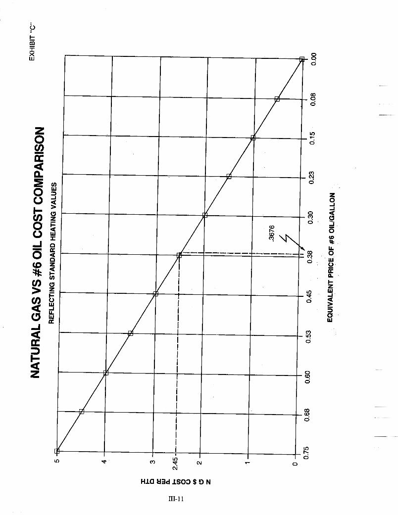
L - m r X w

F

I

a0

0 @?

v)

0 t

0

0 (9 i

1 1 I

I

0 m v ) t cu l-

cu

Hla U3d IS03 $ 9 N

co 0 (9

v) h 1 0

111- 1 1

4-1

I + 0: w 0 3 -

n 3

2.45 - G o o

w 8 2 - z

1 -

0 -

NATURAL GAS VS WASTE OIL REFLECTING STANDARD HEATING VALUES

EXHIBIT “D”

0.58 0.51 0.44 0.37 0.29 0.22 0.1 5 0.73 0.66

EQUIVALENT PRICE OF WASTE OIUGALLON

1

0.07 0.00

EXHIBIT “E” NATURAL GAS VS VARIOUS FUELS

REFLECTING STANDARD HEATING VALUES

5.00 4.50 4.00 3.50 3.00 2.56 2.00 1.50 1 .oo 0.50 0.00

COST/DTH FOR NATURAL GAS 0 #2 OIL + #60IL 0 WASTE OIL

EXHIBIT “F”

5 ,

4

3

2.45

2

1

0

\

NATURAL GAS VS COAL REFLECTING STANDARD HEATING VALUES

I

1

I I I I I

I I

I

I J I

\

I

130 117 104 91 78 65 52 39 26 13 0

EQUIVALENT PRICE OF COAL/TON

1

TABLE III-A

Cost Per Hour For Typical Diesel Generators

Fuel Diesel Generator Size $/Hr. 50 KW $ 2.70 100 KW 5.1 0 250 KW 11.40 500 KW 19.50 750 KW 33.00 900 KW 45.00

Maint. UHr.

Ownership YHr.

$0.50 1 .oo 2.50 5.00 7.50 9.00

$0.54 0.75 1.13 2.08 3.54 5.00

Total $/Hr.

$ 3.74 6.85 15.03 26.58 44.04 59.00

(1) 63 $0.60@al. See Table 111-8

(2) Based on $0.01 per KWH [Le. (50 KW) x (0.01) x (1 Hour) = $0.501

(3) Nominal value only. Wide variations in this factor are expected, depending on whether the machine is new or used and installation. Based on 24,000 hour life expectancy.

TABLE III-B

Cost and Fuel Usage Of Typical Diesel Generators

Diesel Generator Size 1988 List Price Gal/Hr 50 KW $ 1 1 ,000-$ 13,000 4-5 100 KW 15,000- 18,000 8-9 250 KW 23,000- 27,000 18-20 500 KW 44,000- 50,000 30-35 750 KW 80,000- 85,000 53-57 900 KW 100,000- 120,000 73-77

III- 15

i

SECTION IV INDUSTRIAL ENERGY GROUPS

AND STATE STONE ASSOCIATIONS

Industrial Energy Groups

There are regulatory issues that should also be of concern to all of us. Issues that relate to gas, electricity, telephone, etc. that are regulated by your state regulatory commission should be thoroughly scrutinized. Whenever the utility company wants to increase rates, change the rate structure or change anything that may impact your service, they must go before the commission for approval. It is incumbent on each producer to have a voice in the energy structure that the utility plans to impose. If you do not exercise this opportunity you may pay dearly for it.

It’s probably no surprise to most that industrials are subsidizing other classes of customers. Not often do you find all classes carrying theirfull cosf of service. Parity for all should be the goal of the industrials. Even within the industrial arena you may find sweetheart contracts for others that could have a negative impact on your rate. No one should have to subsidize another.

The most effective way to analyze and prepare a good position on any rate or adjustment case brought before the commission by a utility is to unite with an established industrial energy group in your area that exists for just such purposes. If one doesn’t exist, ad-hoc groups can be established to share expenses and to present a unified front. In most cases, professionals are obtained to coordinate and present the opinioils of the group. If your voice is not heard, the commission may assume that the industrial sector is satisfied with the submitted request and rule accordingly.

In order to assist the members in this area a partial listing of known energy groups is presented for your review. It may be beneficial to contract one listed in your area or investigate the possibility of others not listed.

ENERGY GROUPS

STATE GROUP NAME TYPE CONTACT TELEPHONE # 1. Alabama

2. Alaska

3. Arizona

4. Arkansas

5. California California Manufacturers Assn. (CMA) Formal Bob Burt 916-441-5420 Karen Lindh

California Industrial Energy Consumers Ad-Hoc Phillip Stohr 916-441-1031 Industrial Users Ad-Hoc Phillip Stohr 916-441-1031

California Large Energy Consumer Assn Narrow Richard Berby 41 5-271 -21 23

California Industrial Group (CIG) Ad-Hoc Keith McCrae 209-626-661 4 Formal

6. Colorado

7. Connecticut New England Energy Group (NEEG) Formal Jack Lahey 61 7-542-21 00 8. Delaware

9. Florida ~~~~~~

10. Georgia Georgia Industrial Group Formal Chris Hagy 404-658-8700 11. Hawaii

12. Idaho

13. Illinois Illinois Industrial Shipper Group (IISG) Formal Randall Robertson 61 8-876-8500 Illinois Industrial Energy Consumers Group (IIEC) Ad-Hoc Randall Robertson 618-876-8500

14. Indiana (See also Ohio) Firm Robert Hartley 31 7-924-6700

15. Iowa

16. Kansas

17. Kentucky Ad-Hoc David Boehm 51 3-621 -1 045 18. Louisiana (See also Pennsylvania) Ad-Hoc Henry McNicholes 71 7-232-8000

19. Maine See NEEG-New England Energy Group Formal Jack Lahey 61 7-542-21 00

20. Maryland Maryland Industrial Group (MIG) Formal Jack Campbell 301 -563-5679 301 -685-1 71 7

Robert Bair 301-244-7460

21. Massachusetts The Energy Consortium Ad-Hoc David Bell,Ch. 617-227-8010

Ad-HOC

Multi-State

John Hardwicke

Andrew Newman Attorney

See also NEEG-New England Energy Group Multi-State Jack Lahey 61 7-542-21 00 Formal

IV- 1

22. Michigan Association of Businesses Advocating Formal Douglas West 313-259-3232 Tariff Eauitv (ABATE) Attornev

23. Minnesota

24. MississiDDi

25. Missouri

96. Montana ~ ~

27. Nebraska

28. Nevada 29. New Hampshire See NEEG-New England Energy Group Formal Jack Lahey 61 7-542-21 00

30. New Jersey New Jersey Industrial Energy Users (NJIEU) Formal Chris Griemel, 201 -831 -2389

Bill Watkins, 201 -233-6800

Multi-State

Chairman

Attorney

31. New Mexico 32. New York Multi Intervenor Formal AI White 518-434-1161

33. North Carolina Carolina Utility Customer Assn (CUCA) Formal Jerry Roberts, Director 91 9-782-7843

34. North Dakota 35. Ohio (See also Indiana) Firm David Boehm 513-621-1045

Attorney

Ad-HOC Attornev ~~ ~

36 Oklahoma

37. Oregon Also see Washington. Northwest Industrial Gas Users (NIGU)

Industrial Customers of Northwest Utilities (ICNU) Electricity

Assn of Public Aging Customers (APAC) (9 large members)

Private Owned Utilities

TeleDhone Interest

Allen Garten 503-221 -1 440 Ad-HOC Mary Ann Hutton, 503-981 -5095

Ad-HOC Ken Cannon 503-239-91 69 Attorney

Formal Mark Hoehne 206-425-1 550

Private Rog Small 503-635-971 1 Utilities Ad-HOC Jack Landan 503-226-1 191

~~~ ~

38. Pennsylvania (See also Louisiana) Ad Hoc David Boehm 513-621 -1045

39. Rhode Island (See New England Energy Group-NEEG) Multi-State Jack Lahey 61 7-542-21 00

State Group? Formal Andrew Weicker 401 -823-2243

John Bowen, Atty. 803-799-9800 RalDh Millarv 608-257-9521

Formal

40. South Carolina South Carolina Users Committee Formal Ron Cash, Dir.

~~~~ ~

41. South Dakota

42. Tennessee 43. Texas Texas Industrial Energy Consumers Formal Johnathan Day, 71 3-225-701 1

Attorney

44. Utah 45. Vermont See also NEEG-(New England Energy Group) Multi-State Jack Lahey 61 7-542-21 00

Formal

46. Viroinia Viroinia Committee For Fair Utilitv Rates Formal A.C. EDDS. Attornev 804-644-7851

47. Washington See Oregon (#37)

48. West Virginia 49. Wisconsin Ad-HOC Mike Stewart 608-257-9521

50. Wvomina ~~~ ~

GENERAL NOTES 51. NEEG-

Elcon- PGC-

New England Energy Group Formal Jack Lahey, Attorney 617-542-2100 6 states in N.E.

National Electric Group Natural Gas

W. E. Rogers

2806N 8-3-88

IV-2

State Stone Associations

In addition to energy matters, industry is also confronted with many political, environmental and other regulatory problems. For the convenience of the members the National Stone Association has provided a list of the state associations and the name and address of the contact person. In order to protect your interest and to develop a good relationship with allied industrials it would be very advantageous for each NSA member to become affiliated with a state group.

NATIONAL STONE ASSOCIATION 1415 Elliot Place, NW

Washington, DC 20007 (800/342-1415)

(FAX: 202/342-0702)

STATE ASSOCIATION EXECUTIVES

ALABAMA ALABAMA CRUSHED STONE ASSOCIATION, Jim Cunningham, 660 Adams Avenue, Montgomery, Alabama 361 04 205/263-3407

ARIZONA ARIZONA ROCK PRODUCTS ASSOCIATION, Phillip R. Gagle, 420 West Roosevelt St., Suite 10, Phoenix, Arizona 85003 6021271 -0346

CALIFORNIA AGGREGATE PRODUCERS ASSOCIATION OF NORTHERN CALIFORNIA, George H. Cope, 1121 L Street, Suite 1000, Sacramento, California 95814 91 6/443-5353 CENTRAL VALLEY ROCK, SAND AND GRAVEL ASSOCIATION, Linda A. Falasco, P.O. Box 1 11 1, Los Banos, California 93635 209/826-5066 SOUTHERN CALIFORNIA ROCK PRODUCTS ASSOCIATION, Don Reining, P.O. Box 40, South Pasadena, California 91 030 81 8/441-3107

CANADA AGGREGATE PRODUCERS ASSOCIATION OF ONTARIO, Robert P. Cook, 325 Eddystone Avenue, Downsview, Ontario M3N 1 H 8 Canada 41 6/743-5121 LES PRODUCTEURS DE PIERRE A CHAUX DU QUEBEC INC., Roger J. Blais, Agence De Publicite Agrex, Inc., LaSalle Building, 7708 Edouard Street, LaSalle, Quebec H8P 1TP 51 4-363-0851

COLORADO COLORADO ROCK PRODUCTS ASSOCIATION, Jim Sells, 925 South Niagara, Suite 200, Denver, Colorado 80224 303/321-0785

CONNECTICUT CONNECTICUT CRUSHED STONE ASSOCIATION, Donald G. Leavitt, 46 Avery Road, Newington, Connecticut 061 11 203/549-6390

FLORIDA FLORIDA CONCRETE & PRODUCTS ASSOCIATION, INC., Tom Monahan, 649 Vassar Street, Orlando, Florida 32804 3051423-8279 FLORIDA LIMEROCK & AGGREGATE INSTITUTE, INC., Eugene Cowger, P.O. Box 1563, Tallahassee, Florida 32302 904/224-9469

GEORGIA GEORGIA CRUSHED STONE ASSOCIATION, George M. Howard, 3050 Presidential Drive, Suite 21 8, (P.O. Box 941 039) Atlanta, Georgia 30341 4041451-3573

IV-3

ILLINOIS ILLINOIS ASSOCIATION OF AGGREGATE PRODUCERS, George E. Dirkes, 522 West Burlington Avenue, LaGrange, Illinois 60525 312/354-8838

INDIANA INDIANA MINERAL AGGREGATES ASSOCIATION, Joe L. Harrison, P.E., 4905 E. 56th Street, Suite 103, Indianapolis, Indiana 46220 31 7/257-8920

IOWA IOWA LIMESTONE PRODUCERS ASSOCIATION, INC., Ken McNichols, 61 5 East 14th Street, Suite F, Des Moines, Iowa 5031 6-3543 51 51262-8668

KANSAS KANSAS AGGREGATE PRODUCERS ASSOCIATION/KANSAS READY MIX CONCRETE ASSOCIATION, Edward R. Moses, 250 North Rock Road, Suite #340, Wichita, Kansas 67207 31 61687-1 122

KENTUCKY KENTUCKY CRUSHED STONE ASSOCIATION, INC., John W. Sullivan, P.O. Box 326, Frankfort, Kentucky 40602 502/223-2379

LOUISIANA LOUISIANA CRUSHED STONE ASSOCIATION, Ronald M. Madden, P.E., 11823 Market Place, Baton Rouge, LA 7081 6, 504/292-9827 (FAX: 504/292-9260)

MARYLAND MARYLAND AGGREGATES ASSOCIATION, George A. Grier, 2307 Uniontown Road, Westminster, Maryland 21 157 3011876-3751

MASSACHUSETTS MASSACHUSETS CRUSHED STONE ASSOCIATION, % Essex Bituminous Products Company, Attn: John Drislane, 55 Russell Street, Peabody, Massachusetts 01 960 61 7/535-0794

MICHIGAN MICHIGAN MINERAL RESOURCES ASSOCIATION, Doug Graham, 11 16 North Washington Avenue, Lansing, Michigan 48906 51 7/374-8500

MINNESOTA MINNESOTA LIMESTONE PRODUCERS ASSOCIATION, % J.L. Shiely Company, Attn: Mike McCormick, 1 101 North Snelling Avenue, St. Paul, Minnesota 55108 61 2/646-8601

MISSOURI MISSOURI LIMESTONE PRODUCERS ASSOCIATION, INC. Steve Rudloff, P.O. Box 1725 Jefferson City, Missouri 651 02 31 4/635-0208.

NEW JERSEY NEW JERSEY CONCRETE & AGGREGATES ASSOCIATION, William J. Cleary, 770 River Road, West Trenton, NJ 08628 609/771-0099

NEW YORK EMPIRE STATE CONCRETE & AGGREGATE ASSOCIATION, Douglas A. Fuess, 421 New Karner Road, Suite 10, Albany, New York 12205 51 8/456-0036

NORTH CAROLINA NORTH CAROLINA AGGREGATES ASSOCIATION, Fred R. Allen, P.O. Box 30603, Raleigh, North Carolina 27622 91 9/782-7055

OHIO OHIO AGGREGATES ASSOCIATION, Robert A. Wilkinson, 20 South Front Street, Suite 200, Columbus, Ohio 4321 5 61 4/224-2717

IV-4

OKLAHOMA AGGREGATE COMMITlEE, ASSOCIATION OF OKLAHOMA GENERAL CONTRACTORS, Bill Skeith, P.O. Box 53385, Oklahoma City, Oklahoma 73152 405/843-5661

OREGON OREGON CONCRETE & AGGREGATE PRODUCERS ASSOCIATION, Richard L. Angstrom, 3000 Market Street, N.E., #222, Salem, Oregon 97301 503/588-2430

PENNSY LVANlA PENNSYLVANIA AGGREGATES & CONCRETE ASSOCIATION, Kenneth E. Meyer, 3509 North Front Street, Harrisburg, Pennsylvania 171 10 71 7/234-2603

PUERTO RlCO ASSOCIACION DE IND. PROD. DE AGREGADOS, Carlos E. Robles, % Master Enterprises Carr #2, Toa Baja, Puerto Rico 00759 809/785-9255

TENNESSEE TENNESSEE ROAD BUILDERS ASSOCIATION, Bradford Miller, 21 7 6th Avenue North, Nashville, Tennessee 3721 9 61 5/255-5751

TEXAS TEXAS AGGREGATES & CONCRETE ASSOCIATION, Bob R. Beard, 6633 U.S. Highway 290 East, Suite 100, Austin, Texas 78723 51 2/451-5100

VIRGINIA VIRGINIA AGGREGATES ASSOCIATION, INC., James E. Fox, 231 7 Westwood Avenue, Richmond, Virginia 23230 804/353-7464

WASHINGTON WASHINGTON AGGREGATES 81 CONCRETE ASSOCIATION, Roy Bettesworth, 2366 Eastlake Avenue East, #325, Seattle, Washington 981 02 206/329-7744

IV-5

SECTION V ENERGY PUBLICATIONS

UNITED STATES DEPARTMENT OF COMMERCE OFFICE OF ENERGY PROGRAMS

PUBLICATIONS LIST

Brochures listed below are available free of charge when requesting single copies from the Office of Energy Programs or any U.S. Department of Commerce Field Office. Additional copies may be purchased for the prices indicated from the Office of Energy Programs, U.S. Department of Commerce, Washington, D.C. 20230, or the Superintendent of Documents, U.S. Govemment Printing Office, Washington, D.C. 20402. Make check or money order payable to Superintendent of Documents. A 25% discount is available on all orders of 100 or more copies of each brochure when mailed to the same address. The brochures may be reproduced locally, if you so desire.

How to Start an Energy Management Program. Describes how a practical four-point energy management program can be applied to business operations. Price $.25.

33 Money Saving Ways to Conserve Energy in Your Business ($.25) and Energy Management: Economic Sense for Retailers. Basic guides to energy conservation in small industrial and retail businesses. Price $.30.

Energy Conservation Handbook for Capital Light Industries and Commercial Buildings. Aids in identifying specific steps that can be taken to improve fuel utilization in plant buildings and processes and equipment. Price $.35.

How to Profit by Conserving Energy. Provides a sample energy audit that businesses can use to measure the cost of energy per unit output. No charge-only single copies available.

Energy: Critical Choices Ahead. Brochure based on the film with the same title. Gives story of the U.S. energy supply situation and its equally serious long-term implications. No charge-only single copies available.

SavEnergy Kit for Promoting Energy Conservation. A model public awareness kit with sample promotional materials to be incorporated into your public affairs program. No charge-only single copies available.

Total Energy Management. A practical handbook on energy conservation from the National Electrical Contractors Association and the National Electrical Manufacturers Association. For owners and managers of office buildings and small retail stores. No charge-only single copies available.

Copies of the following publications should be ordered from the Superintendent of Documents:

Energy Conservation Program Guide for Industry and Commerce (EPIC). A comprehensive guide to energy conservation opportunities in almost all types of business operations. Price $2.90 (Order from Superintendent of Documents #C13:11:115).

Making the Most of Your Energy Dollars. Describes simple, cost-saving practices of conserving energy for the home-owner. Price $0.70. (Order from the Superintendent of Documents #C13:53:8).

Energy User News. Up to date prices on fuel, utility rankings, energy dialogue, state-of-the-art energy instrumentation, and latest news on rate cases and energy politics. To subscribe: P.O. Box 1087, Southeastern, PA 19398-1087, Attn: Circulation Dept.

FILM LIST

“Energy: Critical Choices Ahead”-available in 18- and 27-minute versions. A color film that analyzes the nature and order of magnitude of our energy problem, discussing our energy needs between now and the year 2000. Price $125.00 (18 min.) and $175.00 (27 min.).

These films are ideal for personnel briefings, association presentations, and group discussions. Available for purchase from the Office of Energy Programs or loan through either the nearest U.S. Department of Commerce Field Office or film library of Modern Talking Picture Service.

v- 1

OTHER SOURCES

Additional materials on energy are available for other government agencies, particularly the Federal Energy Ad- ministration. The materials range from brief brochures to detailed manuals, and cover topics from car pooling to heating and lighting, to specific industrial processes (e.g., cement, glass, plastics, and paper).

Federal Energy Administration, 13th and Pennsylvania Avenue, N.W., Washington, D.C. 20461: Department of Transportation, 400 7th Street, S.W., Washington, D.C.: Energy Research & Development Administration, 20 Mass. Avenue, N. W., Washington, D.C.

Scientijic Methods to Design Crushing and Screening Plants: a reprint from "Mining Engineering" July, 1977, M.D. Flavel, Crushing and Screening Equipment Division, Allis-Chalmers Corporation.

Tools of Power, Power-SME reprint 76-B-311, C.A. Rowland, Jr., Mining Systems Division, Allis-Chalmers Corporation.

v-2

SECTION VI EQUATIONS, FORMULAS, CONVERSION FACTORS

ELECTRICAL EQUATIONS

EQUATIONS FOR DETERMINING KW, KVA, REACTIVE KVA, HP, PF AND AMPERES

ALTERNATING CURRENT

DESIRED DATA SINGLE PHASE THREEPHASE DIRECT CURRENT Kilowatts

KVA

REACTIVE KVA

HORSEPOWER (Output)

AMPERES (When Horse- power is known)

AMPERES (When KVA is

(Volts)(Amps)P.F. 1000

(Volts)(Amps) 1000

(Volts)(Amps) d(P.F.)2’ 1000

(Volts)(Amps)( Eff .)( P.F.) (746)( 1 00)

(HP)(746)( 1 00) (Volts)( Eff .)( P.F.)

(KVA)( 1000) (Volts)

1.73 (Volts)(Amps)P.F. (Volts)(Amps) 1000 1000

1.73 (Volts)(Amps) 1000

1.73 (Volts)(Amps) d(P.F.)2 1000

1.73 (Volts)(Amps)(Eff .)(P.F.) (746) ( 1 00)

(HP)(746)(100) (1.73)( Volts)( Eff .)( P.F.)

(Volts) (Amps) ( Eff . ) (746)( 100)

x

(H P) (746)( 1 00) (Volts)(Eff.)

(KVA)(lOOO) (1.73)(Volts)

known)

VI- 1

Kilowatts KVA

POWER FACTOR =

Kilowatts X lo00 (for 3-phase) 1.73 X Volts X Amps

POWER FACTOR =

Horsepower X 0.746 X 100 Efficiency

MOTOR KILOWATTS =

Horsepower x 0.746 x 100 - MOTOR KVA = - Kilowatts Power Factor Efficiency x Power Factor

5250 X Full-Load Horsepower Speed in RPM

MOTOR FULL-LOAD TORQUE =

7200 Number of Poles

- - 120 X Frequency Number of Poles

SYNCHRONOUS SPEED IN RPM =

Single-phase, Two-wire: Kva = Volts across wires X amperes in one wire t 1000.

Single-phase, Three-wire (Balanced): Kva=Volts across neutral to outside wire x amperes in outside wire X 2 1000.

Three-phase, Three-wire (Balanced): Kva = Volts across any two wires X amperes in any wire X 1.732 f 1OOO.

Three-phase, Three-wire (Unbalanced): Kva = Volts across any two wires X average of the amperes in the three wires X 1.732 t 1000.

Three-phase, Four-wire (Balanced): Kva = Volts across any outside wire to neutral wire X amperes in any outside wire x 3 +- 1000.

Three-phase, Four-wire (Unbalanced): Kva = Volts across any outside wire to neutral wire X average of the amperes in three outside wires X 3 t 1000.

VI-2

ILLUMINATION LEVELS

For Outdoor Lighting

Outdoor R O C ~ E ~ O N I and Sports Frtillles

The lighting installation should be designed and the luminaire selected on the basis of minimum maintained light levels, rather than initial values.

Ylnimum Average Racommsnded Footcandhs*

ILLUMINATION LEVELS-ROADWAYS Vabcutar Roadway Commercial Intermediale Re 1 kkm I i a 1

Footcandle Foolcandle Fwtundh Freeway Expressway Malor 2 0 Collector 1 2 0 9 0 6 Local 0 9 0 6 0 4 Alleys 0 6 0 4 0 4

Tournament Recreational Badminton Tournament Club Recreational Baseball

Regulation Jr League

t o 5

30 20 10

Inlleld Ounleld

30 20 General Application Minimum Average Racommended Foolcandies.

Hangar aprons to approx 50 feet out I Service amons lo amrox 200 feet out I I Center of aircraft sirvice area I

Bedford or butf limestone. smooth buff face brick.

Smooth or medium gray brick. common tan or concrete. aluminum

I Bulletin and Poster Boards I

Buildlna Exleriors I 2 0 (Vertical)

Terra cotla. liqht marble or Dlaster I

I dark field gray brick

surfaces Brownstone, slained wooden shingles. other dark

lndustrlal Yard Material Handling Loading Unloading Platforms. Freight Docks Malls Parks and Gardens Parking Areas Inadstrial N = l n

Hangar aprons to approx 50 feet out Service aprons lo approx 200 feet out Center of aircraft service area Building Exleriors

Bedford Or buff limestone. Smooth buff face brick.

Smooth or medium gray brick. common tan or

Brownstone, slained wooden shingles. other dark

Bulletin and Poster Boards

Terra cotla. light marble or plaster

concrete. aluminum

dark field gray brick

surfaces

1 0 0 5

2 0 (Vertical)

City Suburban 'Runt

15 to 5

20 15 t o

30 20 15

50 35 20

Recreation 70

Entrances laclo,e) Entrances lnormally Ioc*ea nfrequenlly Lsedl Vrta locallons or SlrLCILres. proson yards B L ~ nq sdrrounds

Casting Pool and Area, Ball or Fly croquet Tournament Recreational Football (Index distance from nearest sideline to

Class I: over 100 feet Class 11: 50 feet to 100 feet Class 111: 30 feet to 50 feet Class IV: under 30 feet Class V: no fixed seating

farthest row of spectators)

Golf Courses Driving range Miniature

5 1 5 1

Pier-10, Target-5

to 5

100 50 30 20 to

Grwn or Tee Fairw~ys 5 3 (vertical)

10 5 (vertical) 3 "

Bright surroundings. light surfaces Bright surroundings. dark surfaces Dark surroundings, light surfaces Dark surroundings. dark surfaces Central Station Catwalks Cinder dumps Coal storage area Coal yards (protective) Constructlon General

50 100 20 50

2 0 1 0 1

0 2

i n Excavation Industrial Roadways Adjacent to buildings Not bordered by buildinqs

Active I Inactive

2

1 0 0 5

20 1

Putting green ," to

Club 20 Recredtional t o

Amateur 20 Recreational 10

Tournament to

Lacrosse 20

Hockey, Ice (Rink 65 feet x 200 feet) Professional 50

Horseshoe Pitching

Recreational 5

Marines 1

Playgrounds 5 Raclng Auto. Horse, Motorcycle 20

Dragstrip (staging, acceleration 10.20

Bicycle (touring, competition, recreational) Dog 30

30, 20. 10

deceleration 1st-2nd 660 feet shutdown 620 feet) 5

15, 10

Rifle and Pistol Range Firing point. range, target Rodeos Professional. amateur. recreational Shuffle Board

Recreational 5

Skating Rink 5 P " d

10, 5, 50 (vertical)

50. 30, 10

Tournament 10

I . - I Shoooino centers I 7.6

h;ajor League

Semi-pro and municipal Recreational Combination-baseball. football 20

Basketball Regulation 20

Shopping centers Commercial lots (open, sheltered) Passenger Platforms Protective

. - 2-5 2-5

20

On water to 150 feet out I On beach 100 feet wide

COmmer&Il lots (open, sheltered) Passenger Platforms Protective

- - 2-5

20

All Switch Points Hump area-side of car for reading numbers inspection pit underneath car Shipyards General WaW

2 20 (vertical) 20 (vertical

5 *"

. I Skeet and Trap Shooting-Firing, Target I 5, 30 Skl S low I

Fa&ation areas ," 30

I I G.E. Product Catalog # GEP-635E Dala sublecl lo change wlthoui nmce

Advertising Messages

VI-3

and post boards

Used Car Lots Front Line-first 20 feet of lot Remaining area

100-500 20-75

Soccer Softball

Semi-pro

Swimmlng Pools. Water Surface and Aprons

Prolessional or championship

Industrial League Recreational

Tennis Courts Tournament Club Recreational Volleyball Tournament Recreational

See Football

Infield outtieid

50 30 30 20 20 15 10 7

10

30 20 to

20 I n

SECTION VII DEMAND AND ENERGY SAVINGS

!

SECTION VII: DEMAND AND ENERGY SAVINGS The purpose for this study is to determine the power cost and demand of a typical automated aggregate plant in the southeast and how to reduce this cost. With power costs rising, and this being the second highest cost on an aggregate plant’s financial statement, managers have to consider alternative methods of operating their plants in order to reduce costs.

The typical automated plant in Figure I that we have designed, will have the capability of operating in three separate segments. Each section will be able to operate independently from the others. The first segment is the primary, which will consist of the primary through the surgepile. The second segment is the finishing plant, which will consist of the surge tunnel through to the stockpiles, and the third segment is the load-out, which will consist of the blending tunnels through to the loading bins and classifier. This plant will produce I .8 million tons per year at a 90 percent availability from the primary (1 ,OOO tonshour) and the finishing plant (500 tondhour).

The power charges incurred by an industrial service, such as an aggregate plant, are derived from the schedule “PL-7-1s” (Appendix IV). In order to make this service benefit the aggregate producer, the managers have to operate smarter. Also, new plants need to be‘designed to have the capability to run in segments over three shifts.

Figure 2 is a plan layout of the aggregate plant that we have described. Listed in Appendix I are the horsepowers required to operate this plant. To determine the peak demand, you would take the total horsepower, which is 2,610, and multiply that by a .745699 conversion factor to determine the peak kilowatt demand. Therefore, the kilowatt demand for this plant is 1,946 kw when all three segments are operating together.

In order to meet the market demand of 1.8 million tons per year, the aggregate plant will have to operate the primary plant eight hours per day, 21.67 days per month. The finishing plant will have to operate two eight-hour shifts per day, 21.67 days per month. The load-out will operate on a set 10 hours per day, 21.67 days per month to meet the customer needs. There is a 90 percent overall availability figure built in to take into account mechanical and electrical breakdowns, acts of God, etc.

Five scenarios have been developed for this study. The first scenario (p. VII-5) is to run the primary, finishing plant and load-out one eight-hour shift, or 173.33 block hours per month. As you know by the previous criteria, the finishing plant cannot meet the market demand by operating one eight-hour shift. Also, the load-out will have to operate 10 hours per day to meet the customer needs. The purpose of Scenario No. 1 is for cost comparison only. Operating by this schedule, the kilowatt demand would be 1,946 kw. The operating costs for this 173.33 hours per month would be $28,835.95, as shown on p. VII-5.

In Scenario No. 2 (p. VII-6) the aggegate plant will operate two eight-hour shifts, or 252 block hours per month. This will enable the finishing plant to meet the market demand and will allow the load-out to be open 10 hours. The primary in this case will only have to operate eight hours per day to meet the finishing plant’s demand. Therefore, the peak demand is still 1,946 kw. The operating cost for this schedule is $35,352 per month. This is only a $6,516 increase over one eight-hour shift and only a 22 percent increase in cost, while a 100 percent increase in operating time of the finishing plant and a 25 percent increase in operating time of the load-out.

What these two scenarios have shown us is an increased operating time of 46 percent (block hours), and only a 22 percent increase in power cost. Therefore, what we need to do to reduce power costs using this previous criteria, is to decrease the peak demand and stagger the operation time of each segment. This can be done two ways using a five-day work week.

This brings us to Scenario No. 3 (p. VII-7). We have reduced the peak demand by 44 percent, staggered the operating time of the plant segments, and we are operating 24 hours a day. This reduced the peak demand to 1,100 kw and the monthly operating costs to $27,234, a saving of $8,118 per month. This is in comparison to Scenario No. 2 (shown in Appendix 111), which also fits our production and market criteria.

Finally, Scenario No. 4 (p. VII-8) would be the most economical, but one must consider operating the primary at night. There are several reasons why this might not be possible: (1) safety of equipment operators at night; and (2) noise levels higher than permitted. The cost of lighting the primary will possibly pay for itself. If one can overcome these considerations and operate the schedule under Scenario No. 4, the peak demand will be 1,032 kw. Therefore, the operating cost of this scenario is $26,482 per month. The cost savings per month, year, and ton of No. 4 over No. 2 and No. 3 are shown in Appendix 111.

VII- 1

Another alternative to the conventional industrial power service is the interruptible power service as explained in Scenario No. 5 (pp. VII-9 and 10) and Appendix V. By operating under this service and under the operating schedule in Scenario No. 3, the monthly power cost would be $27,068. These cost savings are also included in the cost comparison in Appendix III. Listed in Appendix 11 is a summary of operating scenarios No. 1 - No. 5 .

This study has shown that there is a tremendous power cost savings by segmenting an automated aggregate plant and by operating 24 hours per day. In return, the peak kilowatt demand and your power cost will be reduced. The final analysis has shown a 25 percent (Scenario No. 4), 23 percent (Scenario No. 3), or a 23 percent (Scenario No. 5) power cost savings over the conventional non-segmented aggregate plant (Scenario No. 2).

VII-2

L

I

i

VII-3

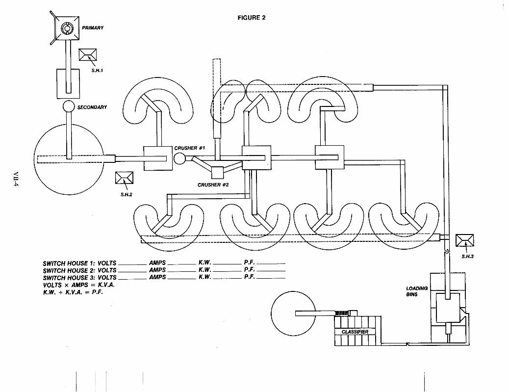
FIGURE 2

SWlTCH HOUSE 1: VOLTS AMPS K. W. P.F. SWlTCH HOUSE 2: VOLTS AMPS K. W. P.F. SWlTCH HOUSE 3: WOLTS AMPS K. W. P.F. VOLTS x AMPS = K.V.A. K.W. + K.V.A. = P.F.

LOADING BINS

I

SCENARIO NO. 1

AUTOMATED AGGREGATE PLANT

HRS.MIK. OPERATING TIMES 40 40 40

8 A.M. - 4 P.M. 8 A.M. - 4 P.M. 8 A.M. - 4 P.M.

PEAK DEMAND PRIMARY -914 kw FINISHING - 846 kw LOAD-OUT- 186 kw

Peak Demand = 914 kw + 846 kw + 186 kw = 1946 kw kwh Consumption:

1946 kw Demand x 173.33 HrsIMonth = 337,300 kwh

kw Hrs. Used -337,300 Billing Demand - 1946 Actual Demand - 1946 Estimated RKVA - 1751

MONTHLY POWER BILL CALCULATION Using Short-cut Formula Method

19

-TO- Service Period

SCENARIO NO. 1

0.01 61 85 c/KWH Fuel Cost Recoverv

FROM BILL:

Kw Billing/Demand KWH Consumption RKVA Actual KW 1946 KW 337,300 KWH 1751 RKVA 1946 KW

piZJ lRKVA[ B WI 337,300 173.3 Hours Use

of Demand 1) Calculate Hours Use of Demand: - - =- pGG1- 1946

2) Determine appropriate category on short-cut formula sheet - Under 200 Hours Use of Demand - Over 200 Hours Use of Demand (but less than 400 Hours Use of Demand) - Over 400 Hours Use of Demand (but less than 600 Hours Use of Demand) - Over 600 Hours Use of Demand

3) Locate appropriate KWD or KWH range in category selected above.

4) Correction Factor from Table - - $ 3,923.85 .................................................................................. S/KWD .................................................................. - 5) + Demand Charge: - x - - $ W[

from table

337,300 5.43 = $ 18,315.39 6) + Energy Charge: x - + (1 OO@/$) ............................................. lKWHl cKWH -

from table

337,300 0.01 61 85 = $ 5,459.20 7) + Fuel Cost Recovery Charge: X ........................................ Wl (1751) 1 102.33 = $ 297.63

x $0.27 8) + Excess RKVA ...........................

Use Only If SUB-TOTAL $ 27,996.07 Positive + 3 %TAX 839.88

(Drop Decimal) TOTAL $ 28,835.95

VII-5

SCENARIO NO. 2

AUTOMATED AGGREGATE PLANT PEAK DEMAND HRS.MIK. OPERATING TIMES

PRIMARY -914 kw 40 7A.M.- 3 P.M. FINISHING - 846 kw 80 7 A.M. - 11 P.M. LOAD-OUT- 186 kw 50 7A.M.- 5 P.M.

PeakDemand = 914kw + 846kw + 186kw = 1946kw

kwh Consumption: 1946 kw Demand x 173.33 Hrs/Month = 337,300 kwh 1032 kw Demand x 43.33 Hrs/Month = 44,716 kwh

Hrs/Month = 109,980 kwh TOTAL: 491,996 kwh

846 kw Demand x 130

kw Hrs. Used -491,996 Billing Demand - 1946 Actual Demand - 1946 Estimated RKVA - 1751


SCENARIO NO. 2

~ TO - Service Period

0.01 61 85 c/KWH Fuel Cost Recovery

FROM BILL:

Kw Billing/Demand KWH Consumption RKVA Actual KW 491,996 KWH 1751 RKVA 1946 KW 1946 KW

~~~ p G i q ml pmiq ml 491,996 252.8 "Jrs Use

of Demand -- 1) Calculate Hours Use of Demand: - - - - 1946


3) Locate appropriate KWD or KWH range in category selected above. 4) Correction Factor from Table .................................................................................. = $ 3,923.85

1946 8.906 = $ 17,331.08 5) + Demand Charge: - x - S,KWD ..................................................................

(KWD] from table

= $ 4,806.80 + (loot/$) 491,996 0.977 x - ............................................. piq CMWH 6) + Energy Charge:

from table 491,997 0.016185 = $ 7,962.97 ........................................ p q 7) + Fuel Cost Recovery Charge;

I/J x=t = ...........................

I ..

Positive + 3 % TAX $ 1,029.67 I (Drop Decimal)l TOTAL $ 35,352.00

VII-6

SCENARIO NO. 3


PEAK DEMAND HRS.MIK. OPERATING TIMES PRIMARY -914 kw 40 7 A.M. - 3 P.M. FINISHING - 846 kw 80 3 P.M. - 7 A.M. LOAD-OUT- 186 kw 50 7 A.M. - 5 P.M.

Peak Demand = 914 kw + 186 kw = 1100 kw

kwh Consumption: 1100 kw Demand 1032 kw Demand 846 kw Demand

x 173.33 Hrs/Month = 190,633 kwh x 43.33 Hrs/Month = 44,716 kwh x 303.33 Hrs/Month = 256,617 kwh

TOTAL: 491,996 kwh

kw Hrs. Used - 491,996 Billing Demand - 1100 Actual Demand - 1100 Estimated RKVA - 990


19

SCENARIO NO. 3

-TO- Service Period

FROM BILL:

Kw BillindDemand 1100 KW

0.01 61 85 c/KWH Fuel Cost Recovery

491,996 KWH 990 RKVA 1100 KW KWH Consumption RKVA Actual KW

IAKW] k!!!!d 491,996 447.3 Hours Use

Calculate Hours Use of Demand: - - =- of Demand

Determine appropriate category on short-cut formula sheet - Under 200 Hours Use of Demand - Over 200 Hours Use of Demand (but less than 400 Hours Use of Demand) - Over 400 Hours Use of Demand (but less than 600 Hours Use of Demand) - Over 600 Hours Use of Demand

E]- 1100

Locate appropriate KWD or KWH range in category selected above.

.................................................................................. Correction Factor from Table - $ - 3,923.85

1100 10.582 = $ 11,640.20 + Demand Charge: - x - S/KWD .................................................................. from table

491,996 0.558 = $ 2,745.34 + Energy Charge: x - + (lOOqY$) ............................................. pci] CKWH from table

491,996 0.016185 = $ 7,962.97 + Fuel Cost Recovery Charge: ........................................

(990) ( llKll) 623.33 = $ 168.30

Use Only If SUB-TOTAL $ 26,440.66 Positive + 3 %TAX $ 793.22


+ Excess RKVA- - 1/3 x - = - x $0.27 .............................. -1

VII-7

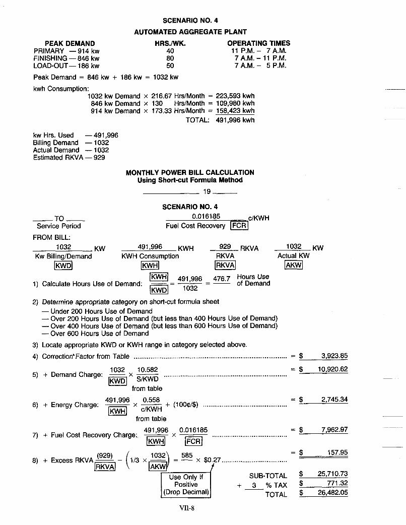
SCENARIO NO. 4


HRS./WK. OPERATING TIMES 40 11 P.M. - 7 A.M. 80 7 A.M. - 11 P.M. 50 7A.M.- 5 P.M.

PEAK DEMAND PRIMARY -914 kw FINISHING - 846 kw LOAD-OUT- 186 kw

Peak Demand = 846 kw + 186 kw = 1032 kw

kwh Consumption: 1032 kw Demand x 216.67 Hrs/Month = 223,593 kwh 846 kw Demand x 130 Hrs/Month = 109,980 kwh 914 kw Demand x 173.33 Hrs/Month = 158,423 kwh

TOTAL: 491,996 kwh

kw Hrs. Used - 491,996 Billing Demand - 1032 Actual Demand - 1032 Estimated RKVA - 929


SCENARIO NO. 4

-TO- Service Period

c/KWH 0.01 61 85 Fuel Cost Recovery

FROM BILL: 1032 KW 491,996 KWH g29 RKVA 1032 KW

Kw Billing/Demand KWH Consumption

[KWD] lKWHl RKVA [RKVAl

Actual KW piG7l

Wl 491,996 476.7 Hours Use of Demand - - - -- Calculate Hours Use of Demand: El- 1032

Determine appropriate category on short-cut formula sheet - Under 200 Hours Use of Demand - Over 200 Hours Use of Demand (but less than 400 Hours Use of Demand) - Over 400 Hours Use of Demand (but less than 600 Hours Use of Demand) - Over 600 Hours Use of Demand

Locate appropriate KWD or KWH range in category selected above. Correction' Factor from Table .................................................................................. = $ 3,923.85

1032 10.582 = $ 10,920.62 Demand Charge: - x - S/KWD ..................................................................

piVD.1 from table

491.996 0.558 . . - - ._. = $ 2,745.34 Energy Charge: ............................................

491,996 0.016185 = $ 7,962.97 ........................................ ~~] Fuel Cost Recovery Charge:,

= $ 157.95 Excess RKVA - (929) - 1/3 x - - - x $0.27 ...................................

SUB-TOTAL $ 259710.73 Positive + 3 %TAX $ 771.32


WJ ( ,+ Use Only If

VII-8

SCENARIO NO. 5 OFF-PEAK DEMAND SHIFTING & BILLING RIDERS

Utility companies usually experience their peak system demand (KW) on a seasonal and hourly basis. In the southeast for example, their peak system demands historically occur during the summer months (June-September), from 1400 hours through 1800 hours, and have become predictable on a daily trend basis.

It is very desirable for the utility to reduce their peak system demand, thereby reducing their fixed and operating costs. The utility is therefore justified in passing on a substantial portion of those savings to the customers who can reduce their KW demand on the required days and hours. These Rate Riders are usually attached to the Standard Rate Schedule.

The Schedule Riders are variously called Time-of-Use (TOU), Off-peak (OP), Variable Off-peak (VOP), etc. and require a voluntary daily demand reduction during the days and hours of the peak summer season. These rider types typically offer 8-12 percent annual savings, but must be strictly adhered to on a daily basis.

Other Schedule Riders such as Supplemental Energy (SE) etc., offer less interruptions and more savings, but require more stringent qualification. Most two-shift operations can qualify for SE type riders, with annual savings of 18- 30 percent. Daily KW trends are monitored by the utility. Only when a peak system demand is predicted for that day will the customer be notified (minimum 30 minutes) of a time and duration (usually 1-2 hours) for his plant KW reduction to a previously contracted level (usually 30 to 60 percent of his normal peak KW). This method substantially reduces the hours of interruption, and the reduced demand KW (by contract) becomes the new contract and billing demand for eight remaining winter months (October through May).

Our example plant can meet market requirements by running 16 hours in the following manner: reduce the normal run 1946 KW demand to a contract 1100 KW for a period of two hours (average). If not exceeded in the peak season, the 1100 KW then also becomes the monthly billing demand for all months annually.

It is readily seen the plant can be run all year at 1946 KW (or more) and billed at 1100 KW, except during the four summer months for a given duration when notified by the utility. Interruptions and duration usually average a total 30 hours in the four months.

COST SUMMARY No. 2 - Standard Rate No. 5 - Interruptible Rate Monthly Savings

$35,352.00 27,067.76

!$ 8,284.24 - 23.4%

VII-9

SCENARIO NO. 5 OFF PEAWINTERRUPTIBLE RATE

Automated Aggregate Plant "Normal Operation @ 16 Hours "Contracted for Demand Reduction to 1100 KW on Interruptible Service Rider

From Scenario 3: Actual Peak Demand Billing Peak Demand Energy

Interruptible Rate: Base Charge First 200,000 KWH @ 0.0739 Next 20,133 KWH @ 0.0543 Next 220,132 KWH @ 0.00977 Next 51,731 KWH @ 0.00558 FCR 491,996 KWH @ 0.016185

Sub Total 3% Sales Tax

Total

PRIMARY Gyratory #1 Belt Scalping Screen Secondary Cone #2 A Belt #2 B Belt #2 C Belt

H.P. 400

175 50 300 100 150 150

1,225

APPENDIX 1

FINISHING #3 Belt

Scalping Screen #4 Belt #5 Belt

Cone Crusher #6 Belt

#1 Screen #7 Belt

Impact Crusher #8 Belt #9 Belt #10 Belt #11 Belt #12 Belt #13 Belt #14 Belt #15 Belt #16 Belt #17 Belt

#2 Screen #18 Belt #19 Belt #20 Belt #21 Belt #22 Belt #23 Belt #24 Belt #25 Belt

1946 KW 1100 KW

491,996 KWH

$ 12.75 14,771.1 0 1,093.22 2,150.69 288.66

7,962.96 $26,279.38

788.38 $27,067.76

H.P. 50 50 20 30 200 40 40 20 250 20 15 20 15 20 10 30 15 30 30 40 15 30 15 30 15 15 30 40

1,135

LOAD OUT #26 Belt #27 Belt #28 Belt #29 Belt

Wash Screen #30 Belt

Fines Pump Sand Screw

#31 Belt

H.P. 40 40 30 30 30 10 30 15 20 245 -

VII- 10

APPENDIX II

OPERATING SCENARIOS

SCENARIO 1st SHIFT 2nd SHIFT 3rd SHIFT TOTAL kw x Hrs/Mo = kwh/Mo kw x Hrs/Mo = kwh/Mo kw x HrslMo = kwh/Mo kwh

#I Primary Finishing Load-Out Totals

#2 Primary Finishing Load-Out Totals




Scenario

Monthly Cost Costrron Yearly Cost Costrron

914 173.33 158,424 846 173.33 146,637 186 173.33 32,239

1946 519.99 337.300 - - -

914 173.33 158,424 846 173.33 146,637 846 173.33 146,637 186 216.66 40,298

1946 563.32 345,359 846 173.33 146.637 - - - - - -

337,300

491,996

914 173.33 158,424

186 216.66 40,298 846 173.33 146,637 846 173.33 146,637

- - - - - - - - - 1100 389.99 198,772 846 173.33 146,637 846 173.33 146,637 491,996

914 173.33 158,424 846 173.33 146,637 846 173.33 146,637 186 216.66 40,298 - - - - - - - - -

1032 389.99 186,935 846 173.33 146,637 914 173.33 158,424 491,996

914 173.33 158,424

186 216,66 40,298 846 173.33 146,637 846 173.33 146,637

- - - - - - - - - 1100 389.99 198,722 846 173.33 146,637 846 173.33 146,637 491,996

APPENDIX 111

COST COMPARISON

No. 1* No. 2 No. 3 No. 4 No. 5

28,836 35,352 27,234 26,482 27,068 .192 .236 .182 .176 .18

346,032 424,224 326,808 31 7,784 324,816 .192 .236 .182 .176 .18

Cost Savings of No. 5 Over Monthly Cost 8,284 166 Costrron .055 .001 Yearly Cost 99,408 1,992 Costrron .055 .001

Cost Savings of No. 4 Over Monthly Cost 8,870 752 Costrron .059 .005 Yearly Cost 106,440 9,024 Costrron ,059 .005

Cost Savings of No. 3 Over Monthly Cost 8,118 CostiTon .054 Yearly Cost 97,416 Costrron .054

*Scenario No. 1 is unrealistic because they do not meet the market demand. It is included for comparative purposes.

VII- 1 1

APPENDIX IV Page Number 4.12 (Superseding Page Number 4.1 Twenty-First Revised

Power and Light Industrial Service

SCHEDULE “PL-7-1s” AVAILABILITY:

Throughout the company’s service area from existing lines of adequate capacity.

APPLICABILITY:

metered at or compensated to that voltage. To all electric service of one standard voltage required on the customer’s premises, delivered at one point and

TYPE OF SERVICE: Single or three phase, 60 hertz, at a standard voltage.

MONTHLY RATE-Energy charge including demand charge: Base charge ............................................................................................................ $12.75 All consumption (kWh) not greater than 200 hours times the billing demand: First 3,000 kWh ......................................................................................... @ 9.81$ per kWh Next 7,000 kWh ........................................................................................ @ 8.94$ per kWh Next 190,000 kWh ..................................................................................... @ 7.29$ per kWh Over 200,000 kWh ..................................................................................... @ 5.43$ per kWh

All consumption (kWh) in excess of 200 hours and not greater than 400 hours times the billing demand ..................................................................... @ 0.977$ per kWh

All consumption (kWh) in excess of 400 hours and not greater than 600 hours times the billing demand ........................... .......................................... 0 0.558$ per kWh

All consumption (kWh) in excess of 600 hours times the billing demand .................................................................................... @ 0.480$ per kWh

Minimum monthly bill: A. $12.75 base charge plus $7.00 per kW of billing demand in excess of 30 kW, plus excess kVAR charges

and fuel cost recovery as applied to the current month kWh.

B. Metered outdoor lighting: The lesser of (1) that determined from paragraph “A” above, or (2) $35.00 per meter plus fuel cost recovery for metered outdoor lighting installations, provided service is limited to the lighting equipment itself and such incidental load as may be required to operate coincidentally with the lighting equipment.

FUEL COST RECOVERY:

Cost Recovery Schedule. The amount calculated at the above rate will be increased under the provisions of the company’s effective Fuel

DETERMINATION OF BILLING DEMAND:

The billing demand shall be based on the highest 30-minute kW measurements during the current month and the preceding eleven (1 1) months. For the billing months of June through September, the billing demand shall be the greatest of (1) the current actual demand or (2) ninety-five percent (95%) of the highest actual demand occurring in any previous applicable summer month or (3) sixty percent (60%) of the highest actual demand occurring in any previous applicable winter month (October through May). For the billing months of October through May, the

VII- 12

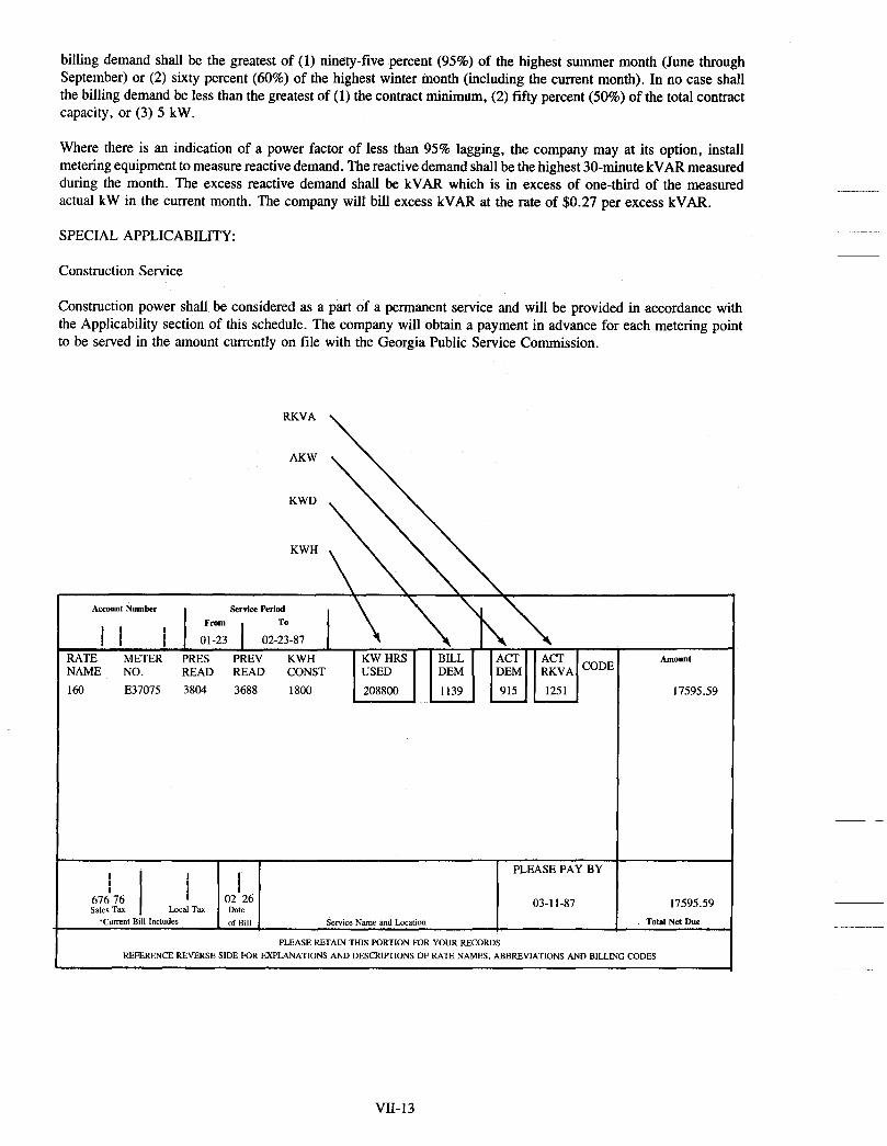
billing demand shall be the greatest of (1) ninety-five percent (95%) of the highest summer month (June through September) or (2) sixty percent (60%) of the highest winter month (including the current month). In no case shall the billing demand be less than the greatest of (1) the contract minimum, (2) fifty percent (50%) of the total contract capacity, or (3) 5 kW.

Where there is an indication of a power factor of less than 95% lagging, the company may at its option, install metering equipment to measure reactive demand. The reactive demand shall be the highest 30-minute kVAR measured during the month. The excess reactive demand shall be kVAR which is in excess of one-third of the measured actual kW in the current month. The company will bill excess kVAR at the rate of $0.27 per excess kVAR.

SPECIAL APPLICABILITY:

Construction Service

Construction power shall be considered as a part of a permanent service and will be provided in accordance with the Applicability section of this schedule. The company will obtain a payment in advance for each metering point to be served in the amount currently on file with the Georgia Public Service Commission.

Account Number Service Period

I Amount

17595.59

17595.59 Tohl Net Due

PLEASE RETAIN THIS PORTION FOR YOUR RECORDS REFERENCE REVERSE SIDE FOR EXPLANATIONS AND DESCRIPTIONS OF RATE NAMES, ABBREVIATIONS AND BILLING CODES

A

VII- 13


-TO- Service Period

19

c/KWH Fuel Cost Recovery

FROM BILL:

KW KWH RKVA KW Kw Billing1Demand KWH Consumption RKVA Actual KW

lKWHl jiGil lAKWl Hours Use of Demand -- 1) Calculate Hours Use of Demand: lKWHl - - -

[iGq -


3) Locate appropriate KWD or KWH range in category selected above.

4) Correction Factor from Table .................................................................................. = $

Demand Charge: - x ~ .................................................................. = $ ml S/KWD - from table

Energy Charge: x - + (lOOqY$) ............................................. = $ m CKWH - from table

Fuel Cost Recovery Charge: X ........................................ = $ pviq ml = $ ...........................

SUB-TOTAL Positive + O/O TAX $

TOTAL !b

VII- 14

APPENDIX V Page Number 6.2 Sixth Revised

(Superseding Page Number 6.2 Fifth Revised)

Supplemental Energy

SCHEDULE “SE-5”

AVAILABILITY:

Throughout the company’s service area from existing lines of adequate capacity.

APPLICABILITY:

This schedule applies in addition to the company’s Off-peak Service Rider conditional to the customer being able to demonstrate and maintain a peak 30-minute demand not less than 1,OOO kW each month and an annual load factor not less than thirty-five percent (35%). The initial load factor shall be based on the month’s load factor in which normal operation occurs or on the annual load factor once twelve months of operating history exists. In either case, the load factor is based on the customer’s maximum actual demand (kW) times the total hours divided into the energy (kWh) used.

The customer will be responsible to the company for any additional cost of installing and removing any equipment required to meter or deliver the requested extra energy.

DEFINITION:

The supplemental energy billed under this schedule shall be the kWh used during the period of supplemental energy availability which results from the product of the current month load factor, the number of hours the customer receives supplemental energy, and the additional demand used. The additional demand used during an on-peak period is determined by calculating the difference between the maximum kW measured during the period of supplemental energy sales and the greater of the maximum kW used on-peak during the period of non-supplemental energy sales or the established billing demand. The additional demand used during an off-peak period is determined by calculating the difference getween the maximum kW measured during the period of supplemental energy sales and the greater of the maximum kW used off-peak during the period of non-supplemental energy sales or the off- peak threshold (billing demand divided by the off-peak ratchet).

CONVERSION OF EXISTING LOAD TO SE LOAD

Existing customers now being served on the company’s standard f i i tariffs (power and light or full-use service to governmental institutions) and who meet all applicability requirements stated under the “Applicability” section above may convert load currently being served on the company’s standard firm tariffs from these standard firm tariffs to the supplemental energy tariff until a maximum of 150,000 kW has been converted. All ratchet provisions contained in the company’s standard firm service tariffs shall be satisfied for any load shifted from the standard f i i tariffs to the supplemental energy tariff.

PROOF OF ABILITY TO REDUCE LOAD:

The customer must demonstrate his ability to interrupt his load to the firm tariff level during each summer that he is subjected to SE interruptions. Failure to interrupt load to the firm tariff level will result in the establishment of a new firm billing demand, subject to the ratchet provisions of the applicable firm tariff.

COGENERATION:

Customers having cogeneration capability shall be required to take service on the company’s limited standby service

VII- 15

rider or the back-up service rider. Supplemental energy shall not be available as a replacement for service on the limited standby service rider or the back-up service rider.

LIMITATION:

This service will be provided if and when the company has supplemental energy available. Supplemental energy will not be available at any time the company’s delivered costs exceed the monthly energy rate plus fuel cost recovery. The company shall have the right to interrupt or deny service under this agreement at any time solely at the option of the company. The minimum notification time for interruption or denial shall be 30 minutes. Usage metered at the customer’s premise during a period of unavailability or interruption shall be billed on the rate under which the customer’s regular service is provided.

LIQUIDATED DAMAGES:

The customer’s actual demand during each continuous period of supplemental energy purchases is limited to the nameplate capacity of the company facilities on the customer’s premise provided for his regular service. The customer shall pay $30.00 per kW per occurrence as liquidated damages for exceeding this limit. The liquidated damages will be applied to the differences between the peak demands established and the nameplate capacity of the company facilities on the customer’s premise provided for his regular service.

TYPE OF SERVICE:

Three phase, 60 hertz, at the voltage the customer’s regular service is provided.

MONTHLY RATE:

Administration charge ...................................................................................... $125 .OO Energy charge ............................................................................................... 1.83 $ per kwh Demand charge (June through September) ............................................................. $ 0.75 per kW

FUEL COST RECOVERY:

The amount calculated at the above rate will be increased under the provisions of the company’s effective fuel cost recovery schedule.

MINIMUM BILLING DEMAND:

The minimum billing demand on the referenced rider shall be ninety-five percent (95%) of the contracted on-peak demand.

Service hereunder subject to rules and regulations for electric service on file with the Public Service Commission.

Effective with service rendered on and after November 2, 1987.

VII- 16

Page Number 9.54 Second Revised (Superseding Page Number 9.54 First Revised)

Supplemental Energy Off-peak Service Rider

SCHEDULE “SEOP-1”

(REVISED)

AVAILABILITY:

Throughout the company’s service area from existing lines of adequate capacity. This rider will be in effect until February 4, 1989.

APPLICABILITY:

Applicable upon request as a modification of the supplemental energy rate schedule, when off-peak usage exists.

RATE:

Off-peak energy charge . . . . . . . . . . . . . . . . . . . . . . . . . . . . . . . . . . . . . . . . . . . . . . . . . . . . . . . . . . . . . . . . . . . . . . . . . . . . . . . . . . . . . . . . . . 1.20$ per kWh

FUEL COST RECOVERY:

The amount calculated at the above rate will be increased under the provisions of the company’s effective fuel cost recovery schedule.

Service hereunder subject to the rules and regulations for electric service on file with the Service Commission.

Public

Effective with service rendered on and after November 2, 1987.

VII- 17

SECTION VIII ENERGY MANAGEMENT

Implementing the Energy Management Program

As another example of applying the energy management techniques developed in the guidelines, the following plant situation was created to better illustrate the implementation of an energy management program. The electrical loads and data will be used from the preceding example.

The following hypothetical plant was developed to show producers how to use the energy guidelines effectively in their own operations. It would be very difficult, if not impossible, to create a set of generic utility rate schedules that would apply to all producers, therefore, the energy committee has attempted to utilize only the basic principles of energy management for this example. A rate analysis was included in this study, using one particular utility, simply to make producers aware that alternate rate schedules and rate riders are available in many areas. Each plant must contact their utility representatives for assistance in rate analysis.

The following example is intended to assist all producers in setting up a functional and effective energy management program by using a step-by-step approach. It is not this committee’s intent for this example to be used to imply, suggest or recommend engineering design criteria, equipment layout or any particular manufacturers equipment.

VIII- I

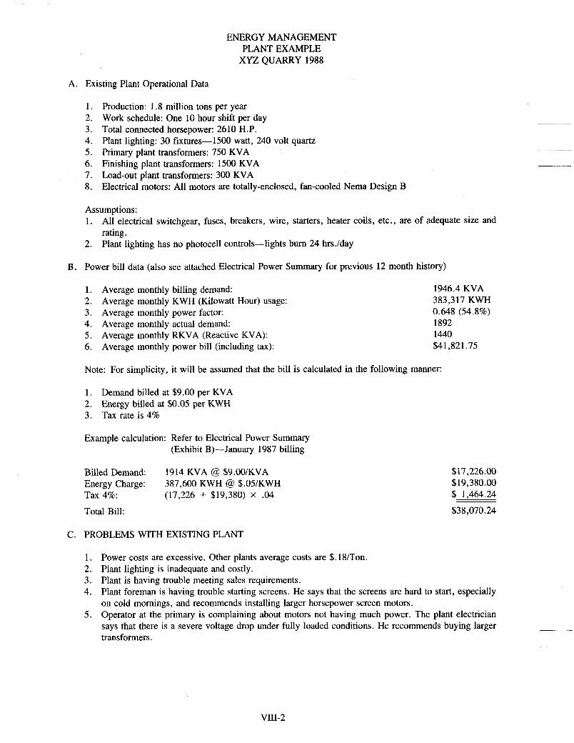
ENERGY MANAGEMENT PLANT EXAMPLE

XYZ QUARRY 1988

A. Existing Plant Operational Data

1. Production: 1.8 million tons per year 2. Work schedule: One 10 hour shift per day 3. Total connected horsepower: 2610 H.P. 4. Plant lighting: 30 fixtures-1500 watt, 240 volt quartz 5 . Primary plant transformers: 750 KVA 6. Finishing plant transformers: 1500 KVA 7. Load-out plant transformers: 300 KVA 8. Electrical motors: All motors are totally-enclosed, fan-cooled Nema Design B

Assumptions: 1. All electrical switchgear, fuses, breakers, wire, starters, heater coils, etc., are of adequate size and

rating. 2. Plant lighting has no photocell controls-lights bum 24 hrs./day

B. Power bill data (also see attached Electrical Power Summary for previous 12 month history)

1. Average monthly billing demand: 2. 3. Average monthly power factor: 4. Average monthly actual demand: 5. Average monthly RKVA (Reactive KVA): 6. Average monthly power bill (including tax):

Average monthly KWH (Kilowatt Hour) usage: 1946.4 KVA 383,317 KWH 0.648 (54.8%) 1892 1440 $41,821.75

Note: For simplicity, it will be assumed that the bill is calculated in the following manner:

1. Demand billed at $9.00 per KVA 2. Energy billed at $0.05 per KWH 3. Tax rate is 4%

Example calculation: Refer to Electrical Power Summary (Exhibit B)-January 1987 billing

Billed Demand: Energy Charge: Tax 4%:

Total Bill:

1914 KVA @ $9.00/KVA 387,600 KWH @ $.OWKWH (17,226 + $19,380) x .04

$17,226.00 $19,380.00 !$ 1.464.24

$38,070.24

C. PROBLEMS WITH EXISTING PLANT

1. Power costs are excessive. Other plants average costs are $. 18/Ton. 2. Plant lighting is inadequate and costly. 3. Plant is having trouble meeting sales requirements. 4. Plant foreman is having trouble starting screens. He says that the screens are hard to start, especially

on cold mornings, and recommends installing larger horsepower screen motors. 5 . Operator at the primary is complaining about motors not having much power. The plant electrician

says that there is a severe voltage drop under fully loaded conditions. He recommends buying larger transformers.

VIII-2

6. Plant maintenance personnel are complaining about having to change quartz light bulbs every three months. Plant superintendent has noticed that he is spending over $lOOO.OO per year on quartz lamps, not to mention the labor associated with changing bulbs. Operator at load-out plant is complaining about not having enough wash water. He says he needs an additional water pump. The engineering department informs the plant superintendent that the existing 200 H.P. pump is rated for 3000 gallons per minute, which should be more than adequate.

7.

IMPLEMENTING THE ENERGY MANAGEMENT PROGRAM

(SEE GUIDELINES)

A. Analyzing Present Usage

1. Audit goals--let us assume that audit goals have been established. We will attempt to: a. Pinpoint inefficient equipment b. Identify opportunities for energy savings c. Compare energy costs at various operations to determine potential savings d. Assign priorities to various energy saving projects

2. Assigning responsibility-The chief electrician was selected for this project, since he understands the principles and has manpower and monitoring equipment. He was required to spend two days with the local utility representative to review the rate structure and bill calculations. He does have a commitment from top management.

3. Setting up the audit

a. Production Equipment-All conveyors, screens, crushers, and associated devices. Non-production equipment-Turbine pump in pit and plant lighting, since lighting is not required during daylight hours and the turbine pump is used to supply make-up water for the settling ponds only. The ponds are sufficiently sized to provide water to the washing system for a minimum of two days. The plant has been divided into three processes: 1) primary plant 2) finishing plant and 3) load-

A demand analyzer will be used to monitor voltage, current, KW demand, kilowatt hours, reactive KVA, and power factor at each of these three electrical switch houses. An electric energy audit form (Exhibit A) has been completed by the plant electrician on every motor. The energy audit form will be used to give us some idea of the efficiency and cost of each motor. Since our example plant contains electrical motors and equipment only, the electrical power summary (Exhibit B) will be used to evaluate energy use and cost. Remember that utility billing periods may not coincide with calendar months. One other form which may be helpful in understanding how a utility bills its customers is the utility verification record (Exhibit C). This form is a standardized request for information about your power bill. It can be mailed to your local utility to obtain information about your particular rate structure. Some of the questions may not apply to your utility, however, it may prove very useful and will certainly indicate your interest in reducing energy costs.

b. out plant.

c.

d.

B. Using the Information

1. We now have, basically, four (4) forms with which to work. a. Exhibit A-Energy Audit Form b. Exhibit B-Electrical Power Summary c. Exhibit C-utility verification record d. Exhibit D-load profile sent by the utility-we could develop our own if mag-tape printouts are

available

VIII-3

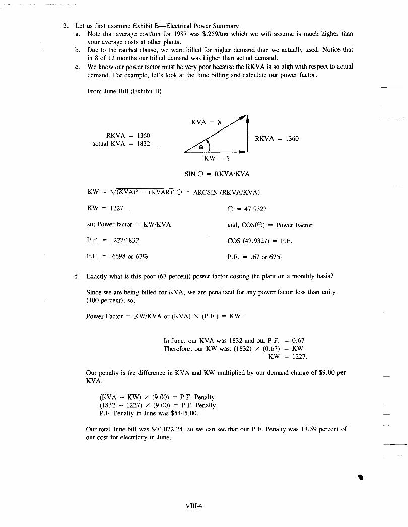
2 . Let us first examine Exhibit B-Electrical Power Summary a.

b.

c.

Note that average cost/ton for 1987 was $.259/ton which we will assume is much higher than your average costs at other plants. Due to the ratchet clause, we were billed for higher demand than we actually used. Notice that in 8 of 12 months our billed demand was higher than actual demand. We know our power factor must be very poor because the RKVA is so high with respect to actual demand. For example, let’s look at the June billing and calculate our power factor.

From June Bill (Exhibit B)

KW = ?

SIN^ = RKVNKVA

KW = V(KVA)~ - (KVAR)’ e = ARCSIN (RKVNKVA)

KW = 1227 e = 47.9327

so; Power factor = KW/KVA and, COS(@) = Power Factor

P.F. = 1227/1832 COS (47.9327) = P.F.

P.F. = .6698 or 67% P.F. = .67 or 67%

d. Exactly what is this poor (67 percent) power factor costing the plant on a monthly basis?

Since we are being billed for KVA, we are penalized for any power factor less than unity (100 percent), so;

Power Factor = KW/KVA or (KVA) X (P.F.) = KW.

In June, our KVA was 1832 and our P.F. = 0.67 Therefore, our KW was: (1832) X (0.67) = KW

KW = 1227.

Our penalty is the difference in KVA and KW multiplied by our demand charge of $9.00 per KVA.

(KVA - KW) X (9.00) = P.F. Penalty (1832 - 1227) X (9.00) = P.F. Penalty P.F. Penalty in June was $5445.00.

Our total June bill was $40,072.24, so we can see that our P.F. Penalty was 13.59 percent of our cost for electricity in June.

VIII-4

e. What can be done to eliminate this penalty?

The penalty cannot be economically eliminated completely, but it can be minimized by adding power factor correction capacitors.

Next, let’s look at the way in which to reduce this costly penalty by adding capacitors.

This is what our power triangle looks like presently (June):

KW = 1227

Suppose we correct our P.F. to 85 percent which would cause our power triangle to look like this:

KW = 1227

We do not know our KVA (x) or our RKVA (y). From the equation COS(0) = P.F. we can solve for these values because we know we want to achieve an 85 percent (.85) P.F.

c o q e ) = P.F.

c o s ( e ) = .85

e = ARCCOS

e = 31.7883

If our angle (e) was 31.7883 then,

(KW) x Tan(0) = RKVA 1227 X TAN (31.7883) = RKVA

RKVA = 760.4

TAN (e) = RKVNKW

If we know that KW = 1227 and RKVA = 760 we can solve for KVA KVA = V(KW)2 + (RKVA)2 KVA = d(1227)’ + (760)2 KVA = 1443.5

VIII-5

Now our P.F. penalty will be:

(1443.5 - 1227) X ($9.00) = P.F. penalty

P.F. penalty = $1948.76, a savings of $3496.24lmo

A simpler way to calculate savings would be to say that, currently, our P.F. is .67 and we want it to be .85.

Since P.F. = KW/KVA and we know our KW = 1227

If P.F. = .85 then .85 = KW/KVA KVA = KWl.85 = 1227/.85 K V A = 1443.5

Our P.F. penalty = (1443.5 - 1227) X ($9.00) = $1948.76

This is a savings of $3496.24

f. The example in e. above showed us the potential savings, but how many capacitors are necessary to correct our P.F. to 85 percent and how much will they cost?

The answer to this question is a bit more tricky and will vary depending on where the capacitors are located and how they are switched. This will depend on your plant electrical system and could be estimated more accurately by your own electrician, engineer, or electrical contractor, but, let’s take a look at some typical numbers.

Our RKVA at 67% (.67) power factor was 1360

Our RKVA at 85% ( . 85 ) power factor was 760

The necessary KVAR (capacitors) to reduce 1360 RKVA to 646 RKVA is simply the difference in the two.

1360 - 760 = 600 KVAR

An average cost for capacitors is $15.00/KVAR depending on quantity and voltage.

(600 KVAR) x ($15.00/KVAR) = $9,000.00

Capacitor Wire & misc. material Switching contactors 4% tax ($35 .OO/M.H. ) Labor

Total

$ 9,000.00 $ 2,000.00 $ 2,500.00 $ 608.40 $ 3,150.00

$17,258.40

This is a lot of money, however, we are going to save $3,496.24 per month. This project will pay for itself in 4.94 months. After that we are looking at bottom line savings.

Now look at our cost/ton if we are saving $3,496.24 per month. Again let’s look at the month of June.

VIII-6

Our power bill is now $40,072.24 - $3,496.24 or $36,576.00. Our production was 134,500 tons, so our cost is now $.2719/ton. We have reduced our costhon by 8.76 percent.

Another alternative to the above power factor calculations could be to install a power factor meter.

3. In reviewing the utility verification record (Exhibit C), which was mailed to and completed by our local utility, we notice that there is a discount for primary metering of $.Ol/KWH (Item E). How can we take advantage of this discount?

Answer: We have two options, 1) build our own substation or 2) purchase the substation from our utility.

We will assume the utility does not wish to sell their substation and we will look at some rough approximations of cost to build our own. Keep in mind that the following cost figures are “ballpark” numbers. A detailed cost estimate should be made by qualified engineers, consultants, contractors, etc., before pursuing a project of this nature.

PRIMARY SUBSTATION 25000 VOLTS12470 VOLTS

COST STUDY 1 ea.-3500 KVA transformer (used or rebuilt) 1 ea.-15KV main breaker (vacuum type) 1 ea.-Gang operated switch (load break) 1 ea.-25 KVA station service transformer 1 ea.-15 KV substation structure (used) Site preparation (75’ x 75’) Substation fence and signs Concrete pad Substation lighting Miscellaneous wire, lugs, conduit, etc. Labor (480 manhours at $35.OO/M.H.)

Total Cost

$35,000.00 $15,000.00 $ 7,000.00 $ 300.00 $ 4,500.00 $ 2,000.00 $ 2,600.00 $ 7,500.00 $ 500.00 $ 4,000.00 $16,800 .OO

$95,200 .OO

From our utility verification record (Exhibit C) and our average monthly KWH consumption of 383, 317 KWH our monthly savings should be approximately $3,833.17.

(383,317) x ($.Ol/KWH) = $3,833.17

This project would pay for itself in approximately 25 months depending on energy consumption. This may or may not be an attractive return but is most definitely a savings worth consideration. If we take advantage of this discount we will save 2.85Won based on June production. Our cost/ton will be lowered by an additional 10.6% bringing the cost down to $.2397/ton, assuming we have already added our power factor correction capacitors.

4. What about plant lighting? Is there a potential for savings?

Yes, we know that there are 30 each of a 1500 watt, 240 volt quartz fixture used for plant lighting. Our energy management team tells us that these lights burn 24 hours per day. Let’s look at costs.

(30 fixtures) x (1500 watts) = 45000 watts or 45 KW

(45 KW) X (24 hours/day) x (30.4 days/mo) = 32,832 KWH

VIII-7

If we were to cut the lights off during daylight hours we would only use:

(45 KW) X (12 hourslday) X (30.4 dayslmonth) = 16,416 KWH For a savings (based on $.05 KWH) of:

(16,416 KWH) X ($.05) = $820.80 per month

Another option, for long range savings, would be to replace these quartz fixtures with high pressure (HID) lighting. Comparing these two types of lighting we have: (see Table 11-M in guidelines)

(30 each) x (1500 watts) x (22 lumenslwatt) = 990,000 lumens

To get approximately the same level of lighting we will need 8 - IOOO-watt HPS floodlights.

(8 each) x (loo0 watt) X (125 lumenslwatt) = 1,OOO,000 lumens

For a cost comparison, consider the following example of the typical costs associated with each type of light.

cost of light per fixture (based on 8760 hours per year)

Lamp cost Labor Electricity

Total

1500 watt quartz 1000 watt H.P.S. $88.00 (4 lamps) $34.00 $40.00 (4 changes) $3.34

$657.00 $438.00

$785.00 $475.34

This is an annual savings of $309.66 per fixture. For our example, using 30 quartz fixtures we are spending approximately $23,550.00 on lighting. By burning the quartz lights only 12 hours per day we can reduce this to $1 1,775.00, but, by replacing the 30 quartz fixtures with 8 high pressure sodium lights our annual cost for lighting will be only $3,802.00 if we bum them 24 hours per day; and we will actually have a little more light. The installed cost of 8 HPS floodlights is approximately $5,500.00 based on installing two (2) power poles with 4 lights per pole. The price per light is about $420.00, which includes lamp and labor to mount. If we consider the present situation, of burning the quartz lights 24 hours per day, and elect to replace the quartz fixtures with HPS, our savings will be about $19,748.00 annually. This is a monthly savings of $1,645.67 which means the $5,500.00 investment will pay for itself in 3.34 months.

5 . Examining the load profile (Exhibit D), which was sent to us by our utility, as we requested in our utility verification record, we can gain some insight as to what our KW demand is doing throughout a typical day of operation.

In looking at the load profile, it is obvious that there are several peaks. These peaks occur at various times during the day. Our highest peak of the day occurs at approximately 1 1.15 AM. But also notice that the peak falls noticeably at 1:00 PM, remains fairly constant until about 4:OO PM, peaks upward again at 4:00 PM and stays up until about 5:30 PM when it drops, remains constant until about 7:OO PM, where it peaks upward again and finally starts dropping about 7:30 PM. Let’s summarize these peaks:

1. Peaks at 11: 15 AM at about 2000 KW 2. Falls sharply at 1:00 PM 3. Remains somewhat constant at 1750 KW from 1:OO - 4:OO PM

VIII-8

4. Peaks at 4:00 PM to about 1900 KW 5. Remains fairly constant until about 5:30 PM 6. Falls sharply at 530 PM 7. Remains constant until about 7:00 PM 8. Peaks at about 7:15 to about 1950 KW 9. Falls at 7:30 PM

10. Continues to fall until about 10:30 PM

What does this information tell us?

Let’s suppose we have checked with our plant operations personnel and they tell us that, on the day of the load profile (July 18, 1987), the maintenance people were working on the 500 H.P. pit turbine pump. While making repairs, the maintenance crew had to start, stop and take amp readings, flow measuFements and other information on the pump. The pit foreman remembers that the pump was started once at 4:OO PM and again at 7:00 PM, but he is not sure about other times. These times correspond to peaks on our load profile. The peaks we have seen are in the 300 KVA range, which is about what our 500 H.P. turbine pump should run (if we have a good power factor). If we can shift this 300 KVA to a time when our plant is not running, we can reduce our peak demand. This will lower our actual demand as well as our billed demand which could save us about $2700.00 per month ($9.00 per KVA X 300 KVA). Why not take advantage of this savings by running the turbine pump at night? If we can pump enough water at night to fill our settling ponds, this should not pose a problem and we will save the $2700.00 per month. As you can see, the load profile has been very helpful in identifying problems and indicating solutions to peak demand control.

6. Let’s solve the primary plant operator’s problem of motors not having much power. The electrician has told us that the voltage is too low under full load conditions. The solution could be found by reviewing the electric energy audit form. Notice that, under “actual operation,” our total amps are 1434 amps, our KW is 751 and our voltage runs about 450 volts. Our power factor, however, is running about 65 percent (.65). We know, from our previous power factor calculations that KVA = KW/P.F., so;

KVA = KW1P.F. KVA = 75U.65 KVA = 1155

Our transformer bank, at the primary, is rated for 750 KVA. We have overloaded this transformer bank by 54 percent. By adding power factor correction capacitors, we can improve this overloaded condition for example, if we correct our P.F. to 90 percent. (.90) our bank of transformers will only see 834.4 KVA.

KVA = 75U.90 KVA = 834.4

Now our transformers are only 11.26 percent overloaded, which has improved our power factor, reduced the P.F. penalty and improved our voltage. By improving our voltage we have increased the torque of our motors. For more information on the function and benefits of capacitors, review section IIB-3 in the guidelines. Pay particular attention to the graph on page 11-10 and notice that as rated voltage decreases, the full load current increases and rated torque goes down. For example, if voltage is running at 90 percent of nameplate rating, then the torque is only 80 percent of what it is rated.

7. Our plant foreman is still having problems starting his screens and still insists that we increase the horsepower of the screen motors. We can see, from our electric energy audit form (Exhibit C), that the screens are pulling close to full load amps. There is no need to increase horsepower, which would only lower the efficiency of our motors. We have several options:

a. Increase the size of heater elements in our overload relay. This could be an easy, inexpensive

VIII-9

solution, provided we do not increase the elements to the point of sacrificing our overload protection of the motor. It would be advisable to check with a knowledgeable person before doing this. The motor manufacturer or distributor can be helpful in this area.

b. Install a timed shunt on the overload relay. This would bypass (jump out) the overload relay for the amount of time to get the motor started only. This may not be inexpensive and could create maintenance problems.

c. Replace the Nema design B motors with an equivalent size Nema design C motor. This would greatly increase the starting torque and is always a good decision when building a new installation. Check with your motor distributor first, because some manufacturers build their Nema B motors to Nema design C specifications. Your motor may be nameplated as Nema design B, but in reality it may be a Nema design C already. See figure 11-E in the guideline for a graph comparing Nema design A, B, C, and D torque curves.

8. Now for the load-out plant operator and his water problem. Our energy management team installed a demand analyzer and a flow meter on the 200 H.P. settling pond pump. Our measurements show that, although, the pump motor seems loaded, we are only pumping about 1500 G.P.M. This is only half of what our engineers say it should pump. A further inspection of the pump revealed a badly wom impellar. After this is done we will take power and flow readings to insure the pumping efficiency. It is not necessary to install an additional pump.

c. summary In the preceeding example, we have attempted to demonstrate how the energy management

guidelines can be effectively put into use in a real plant. Obviously, the applications will differ from plant to plant and utility to utility. Some of the concepts are technical but most are just plain common sense. The main ideas are: 1) do we know how we are using the energy we buy? 2) do we know how much this energy costs? 3) are we using this energy wisely and effectively? and 4) can we reduce these rising energy costs? Energy costs will, most likely, never decrease and it will, most likely, continue to increase. We must decide for ourselves what priority we will place on the four questions above and take positive steps to control these rising costs to run our operations.

Let’s briefly review the problems our energy management team started out trying to solve and see what they accomplished. 1. We corrected the poor power factor ............................................ savings-$3946.00/month 2. We replaced quartz lights with HPS ........................................... savings-$l645.00/month 3. We took advantage of primary metering discount ........................... savings-$3833 .OO/month 4. We are reducing demand by running turbine pump at night ............... savings-$27OO.OO/month

If we apply the total savings (1 thru 4) above to our June bill, we will have reduced that power bill from $40,072.24 down to $28,398.24 which is a cost reduction of 29.1 percent. This is a unit cost savings of $0.0868 per ton, which reduces the June electrical cost from $0.298 per ton to $0.2111 per ton.

Other accomplishments include:

5.

6.

7. 8.

Correcting low power conditions at the primary. This has allowed the operator to increase the production through the primary by feeding more rock, since motors no longer “pull down.” It also will increase the life of motors and we did not spend money on larger transformers. By replacing screen motors with NEMA Design C motors, we did not lose efficiency and we are no longer losing production while trying to start screens. We are no longer spending money on bulbs and labor to change lamps on quartz lighting. Our load-out operator has plenty of wash water and we have not bought an additional pump.

We have invested about $119,668.00 to save $1 1,674.00 per month, which gives us an overall payback of about 9.8 months. This does not include the cost to replace the screen motors since we are putting them into inventory as spares.

VIII- 10

Many steps and approaches can be taken to save money on energy, and this example does not, by any means, cover all possibilities. The intention is only to illustrate what can be achieved through a commitment of effort and funds to a good energy management program.

VIII- 1 1

PRIMARY PLANT ELECTRIC ENERGY AUDIT FORM

s U

+ 7 N

COI (1) x 0.746; (HP x 0.746 = KW) ** COI (6) x COI (5) x 1.732 x P.F. + 1000 = KW

flf P.F. not known. use 0.9 ~ ~~

*** Actual operating data is more meaningful, in energy studies, if one takes no load, average load, and full load readings.

Exhibit A

ELECTRIC

ITEM NAME PLATE DATA

HP AMPS VOLTS KW*

(1 1 (2) (3) (4)

#3 BELT 50 65 480 37

SCALPING SCREEN 50 65 480 37

#4 BELT 20 27 480 15

#5 BELT 30 40 480 22

CONE CRUSHER 200 240 480 149

#6 BELT 40 52 480 30

#1 SCREEN 40 52 480 30

#7 BELT 20 27 480 15

IMPACT CRUSHER 250 31 2 480 187

#8 BELT 20 27 480 15

#9 BELT 15 21 480 11

#10 BELT 20 27 480 15

#11 BELT 15 21 480 11

#12 BELT 20 27 480 15 8

88

888

ENERGY AUDIT FORM

ACTUAL OPERATION*** DIFFERENCES NOTES

AMPS VOLTS KW** AMPS VOLTS KW

(5) (6) (7) (8) (9) (10)

62 480 33 3 0 4

62 480 33 3 0 4

26 480 14 1 0 1

38 480 21 2 0 1

228 480 123 12 0 26

49 480 27 3 0 3

49 480 27 3 0 3

26 480 14 1 0 1

296 480 160 16 0 27

26 480 14 1 0 1

20 480 11 1 0 0

26 480 14 1 0 1

20 480 10 1 0 1

26 480 14 1 0 1

COI (1) x 0.746; (HP x 0.746 = KW) COI (6) x COI (5) x 1.732 x P.F. + 1000 = KW (If P.F. not known, use 0.9 Actual operating data is more meaningful, in energy studies, if one takes no load, average load, and full load readings.

Exhibit A (continued)

I i

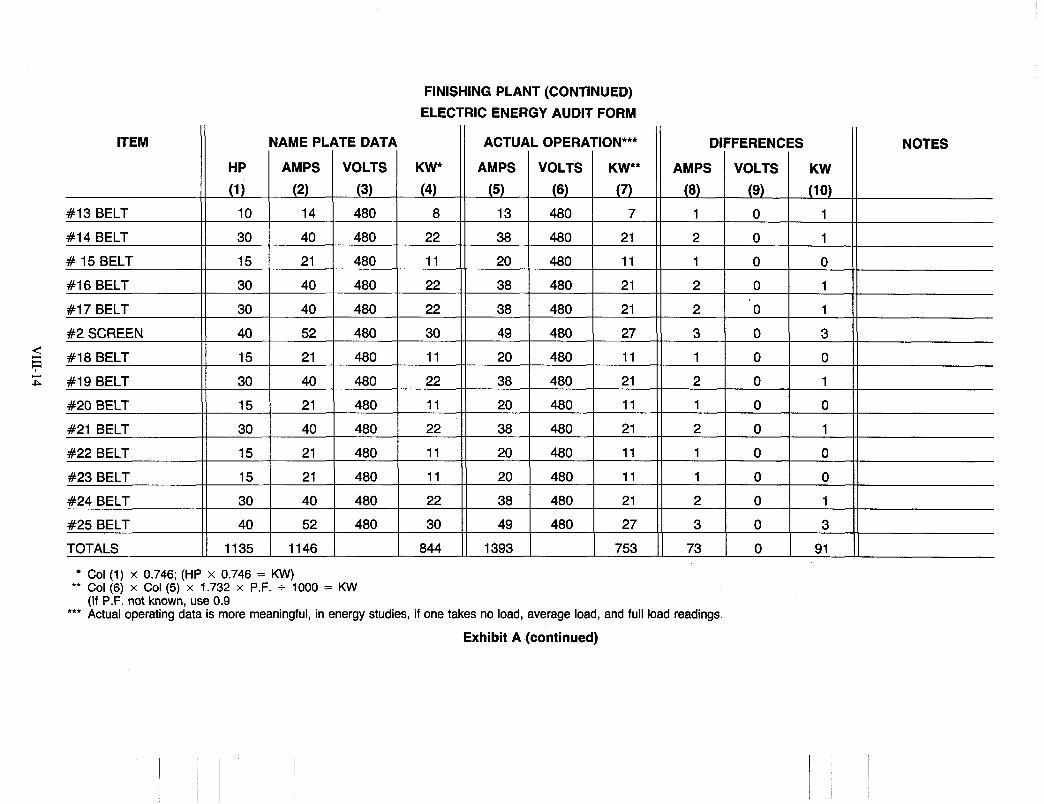
FINISHING PLANT (CONTINUED) ELECTRIC ENERGY AUDIT FORM

ITEM

#13 BELT

#14 BELT

# 15 BELT

#16 BELT

#17 BELT

#2 SCREEN

#18 BELT

#19 BELT

#20 BELT

#21 BELT

#22 BELT

#23 BELT

#24 BELT

#25 BELT

TOTALS

NAME PLATE DATA ACTUAL OPERATION*** DIFFERENCES

HP AMPS VOLTS KW* AMPS VOLTS KW** AMPS VOLTS KW

(1 1 (2) (3) (4) (5) (6) (7) (8) (9) (10)

10 14 480 8 13 480 7 1 0 1

30 40 480 22 38 480 21 2 0 1

30 40 480 22 38 480 21 2 0 1

40 52 480 30 49 480 27 3 0 3

1135 1146 844 1393 753 73 0 91

COI (1) x 0.746; (HP x 0.746 = KW) ** Col (6) x Cot (5) x 1.732 x P.F. + 1000 = KW

*** Actual operating data is more meaningful, in energy studies, if one takes no load, average load, and full load readings. (If P.F. not known, use 0.9


NOTES

LOAD OUT PLANT ELECTRIC ENERGY AUDIT FORM

NAME PLATE DATA

HP AMPS VOLTS KW*

(1) (2) (3) (4)

#26 BELT 40 52 480 30

#27 BELT 40 52 480 30

#28 BELT 30 40 480 22

#29 BELT 30 40 480 22

WASH SCREEN 30 40 480 22

#30 BELT 10 14 480 8 2 ? FINESPUMP 30 40 480 22

SAND SCREW 15 21 480 1 1

#31 BELT 20 27 480 15

v1

TOTALS 245 326 182

NOTES ACTUAL OPERATION*** DIFFERENCES

AMPS VOLTS KW** AMPS VOLTS KW

(5) (6) (7) (8) (9) (10)

49 480 27 3 0 3 49 480 27 3 0 3

38 480 21 2 0 1

38 480 21 2 0 1 38 480 21 2 0 1

13 480 7 6 0 1

38 480 21 2 0 1

20 480 1 1 1 0 0

26 480 14 1 0 1

309 170

ITEM

COI (1) x 0.746; (HP x 0.746 = KW) ** Col (6) x Col (5) x 1.732 x P.F. + 1000 = KW

(If P.F. not known, use 0.9 *** Actual operating data is more meaningful, in energy studies, if one takes no load, average load, and full load readings.


OTHER LOADS ELECTRIC ENERGY AUDIT FORM

. OPERATION***

VOLTS 1 KW**

ITEM DIFFERENCES

AMPS I VOLTS I KW

PIT PUMP ITURBINE)

2300

480 SETTLING POND

303 6 100 70

123 12 0 26

TOTALS

200

PLANT LIGHTING

(30 - each 1500 watts

@ 6.25 amps)

240 480 149 228

NAME PLATE DATA 1 1 ACTW

700

1 A F ~ V ( X f S ~ 1 1 A r

500 123 2400 373 117

363 522 345

187.5 240 45 187.5 240 45 1500 WATT, 240 VOLT

QUARTZ FIXTURES

NOTES

426

COI (1) x 0.746; (HP x 0.746 = KW) ** COI (6) x COI (5) x 1.732 x P.F. + 1000 = KW

(If P.F. not known, use 0.9 *** Actual operating data is more meaningful, in energy studies, if one takes no load, average load, and full load readings.


YEAR: 1987

BILL

$38,070.24

$38,702.56

$33,343.44

$33,619.04

$37,505.52

$40,072.24

$44,100.1 6

$42,957.20

ELECTRICAL POWER SUMMARY UTILITY NAME: RKW ELECTRIC CO.

RKVA KWH ACTUAL BILLED OPERATED PRODUCED KWH $.TON TON KVA KVA PENALTY

* 1388 387,600 1827 1914* 21 7 156,000 $0.098 $0.098 2.485 81 S O 202.50 $5373.00

1495 394,000 1946 1946 221 135,000 $0.098 $0.282 2.91 9 69.73 202.50 $6302.26

1440 296,700 1854 191c 21 0 112,000 $0.112 $0.283 2.649 58.52 155.00 $5878.16

141 4 302,000 1840 1914 223 122,903 $0.1 11 $0.274 2.457 64.21 157.80 $561 6.35

1457 376,200 1917 1917 220 11 5,000 $0.1 00 $0.326 3.271 59.99 196.20 $6040.72

1360 426,100 1832 191 4* 237 134,500 $0.094 $0.298 3.1 68 70.27 222.60 $51 05.05

1507 478,000 2056 2056 240 281,000 $0.092 $0.157 1.701 136.70 232.50 $5916.58

1497 471,500 1970 1970 231 201,300 $0.091 $0.21 3 2.342 102.20 239.30 $6204.76

ACCOUNT NUMBER: 61-750014-01

$33,891.28 141 6 41 5,600 1863 1953 205 163,750 $0.096 $0.244 2.538 83.85 212.80 $5471.57

$38,580.88 1468 390,400 1890 1953 21 6 165,000 $0.099 $0.234 2.366 84.49 199.90 $5984.16

$38.757.68 1477 393,800 1922 1953 200 130,000 $0.098 $0.298 3.029 66.56 201.60 $6077.13

$32,210.88 1359 267,900 1788 1953 202 134,000 $0.120 $0.240 1.999 68.61 137.20 $4953.47

$457,811.12 17,278 4,599,800 22,705 23,357 2622 1,850,453 $1.21 1 $3.1 12 30.925 946.23 2360.00 $68,923.21

$38,150.93 1439.8 383,317 1892 1946 21 8.5 154,204 $0.101 $0.259 2.577 78.85 196.70 $5743.60

MONTH

,

-

JAN.

FEB.

MARCH

APRIL

MAY

2 JUNE 7 Ti JULY

AUG.

SEPT.

OCT.

NOV.

DEC.

TOTAL

AVERAGE

TOTAL I 1 I KWH/ 1 TONS/ I KWH/ I P.F.

* 1986 Summer Peak of 2015 (2015) x (0.95) = 1914

Note: Power bills are not usually billed on calendar months, care must be used when evaluating ratios since production reports are normally based on a calendar month.

Exhibit B

!

UTILITY VERIFICATION RECORD Date: 1-5-88

Plant: XY z Utility name: RKW ELECTRIC Address: 1010 Old Quarry Hwy.

Somewhere, U.S.A.

Account no.: 61-750014-01

Utility representative: John Doe Phone no.: (555) 555-5555

Contract date: 6-14-72 Current rate schedule: Large Power User ( Lpu

Power factor clause: Yes (Yes/No) Average power factor: 65%

Service Secondary (Primary/Secondary) Voltage: Primary 25000 Volts Secondary 12470 Volts

No. of meters at this location: 1 Demand basis KVA (KW/KVA) July 2056 478000

Month Demand KWH Highest demand past 12 Months:

Minimum power factor to avoid penalty:

Demand interval: 15 min. (1 5 min./30 min.) Sliding window: No (Yes/No)

A. Which of the following information appears on monthly bill?

100%

H KWH KVA (Billed) 0 Power factor KVA (Actual) 0 KW (Billed) RKVA 0 KW (Actual) 0 Power factor penalty

B. Is there a ratchet associated with this rate schedule?

C. How is monthly power factor determined? Power factor at peak demand

0 Average power factor for billing cycle H Average power factor at three (3) highest peak demand

Power factor calculated using RKVA at highest peak demand 0 Other

Yes (Yes/No)

If other, please explain:

D.

E.

F.

~~

Are mag-tape printouts available? Yes (Y es/No)

Is there a discount for primary metering? Yes (Yes/No)

If yes, what is the discount?

Please attach the following information: 1. Load profile of monthly demand 2. Previous 12 month history 3. Copy of current rate schedule 4. Current fuel adjustment or fuel cost recovery

5. Copy of effective contract

$0 . 0 1 Per KWH

6. Minimum bill calculation 7. How demand is determined 8. Copies of all rate schedules available,

including all available rate riders, such as off

energy, etc. charge peak, time-of-use, interruptable, supplemental

I verify, to the best of my knowledge, that this facility is currently being billed on the most economical rate available.

Utility Representative Date

Return to: XYZ Quarry 1010 Old Quarry Highway

Somewhere, U. S . A. Zip Code Exhibit c VIII- 18

PEAK DAY DEMANDS 2000

1750 1 1600 KVA

0 z

W 1250

n -I

K W I-

w 750 I- 3

5 1000

z

z 500 0

c3

250

0

I I I I I I I I I I I I I I I I I I I I I

0O:OO 02:OO 04:OO 06:OO 08:OO 1O:OO 12:OO 14:OO 16:OO 18:OO 20:OO 22:OO 24:OO

July 18, 1987

Exhibit D

VIII- 19

Date post:	26-May-2018
Category:	Documents
Upload:	vophuc
View:	212 times
Download:	0 times