Enforcement of Vintage Differentiated Regulations: The Case of New Source Review James B. Bushnell and Catherine Wolfram * February 2012 Abstract We analyze the effects of the New Source Review (NSR) environmental regulations on coal- fired electric power plants. Regulations that grew out of the Clean Air Act of 1970 required new electric generating plants to install costly pollution control equipment but exempted existing plants. Plants lost their exemptions if they made “major modifications.” We examine whether this caused firms to invest less in grandfathered plants, possibly leading to lower efficiency and higher emissions. We find evidence that heightened NSR enforcement reduced capital investment at vulnerable plants. However, we find no discernible effect on other inputs or emissions. JEL Classification: L51, L94, Q58, and Q52 Keywords: New Source Review, Environmental Regulations, Productivity, and Electricity * Bushnell: UC Davis and NBER. Email: [email protected]. Wolfram: Haas School of Business, UC Berkeley and NBER. Email: [email protected]. We are grateful to Meredith Fowlie, Michael Greenstone, Erin Mansur, Nancy Rose and Rob Stavins for valuable comments and discussions, and we thank Justin Gallagher, Rob Letzler, Carla Peterman, Amol Phadke, Jenny Shanefelter and Ethan Yeh for excellent research assistance.
Transcript
Enforcement of Vintage Differentiated Regulations: The Case of
New Source Review
James B. Bushnell and Catherine Wolfram∗
February 2012
Abstract
We analyze the effects of the New Source Review (NSR) environmental regulations on coal-fired electric power plants. Regulations that grew out of the Clean Air Act of 1970 requirednew electric generating plants to install costly pollution control equipment but exemptedexisting plants. Plants lost their exemptions if they made “major modifications.” We examinewhether this caused firms to invest less in grandfathered plants, possibly leading to lowerefficiency and higher emissions. We find evidence that heightened NSR enforcement reducedcapital investment at vulnerable plants. However, we find no discernible effect on other inputsor emissions.
JEL Classification: L51, L94, Q58, and Q52 Keywords: New Source Review, EnvironmentalRegulations, Productivity, and Electricity
∗Bushnell: UC Davis and NBER. Email: [email protected]. Wolfram: Haas School of Business, UCBerkeley and NBER. Email: [email protected]. We are grateful to Meredith Fowlie, Michael Greenstone,Erin Mansur, Nancy Rose and Rob Stavins for valuable comments and discussions, and we thank Justin Gallagher,Rob Letzler, Carla Peterman, Amol Phadke, Jenny Shanefelter and Ethan Yeh for excellent research assistance.
1
1 Introduction
Many regulations in the United States apply different standards to new and old units, whether the
units are cars subject to fuel-efficiency standards, buildings subject to building codes, or electric
power plants subject to environmental regulations. This asymmetric regulatory treatment is
known as vintage differentiated regulation (VDR). There are several rationales for using a VDR.
From an efficiency perspective, it is often prohibitively expensive to retrofit existing units with the
new technology, either because the retrofits themselves are expensive or because the transaction
costs involved in running a recall program are prohibitive. From a political perspective, if owners
of existing units are exempt from the new regulation, their incentives to oppose it are limited.
Policymakers envision that over time, new units will replace old ones, so that in the long run,
the universe of units will reflect the new standard.
Previous theoretical and empirical work has shown that vintage differentiated regulations can
lead to several types of distortions in the short run (see Stavins (2006) for an overview of the
literature). First, if the regulations increase the cost of building the new unit, old units will be
kept in service far longer than they would have absent the VDR. For example, previous work
has found some evidence that the Corporate Average Fuel Economy standards for new vehicles
increased sales of used vehicles (Goldberg, 1998). Related to this, in contexts where consumers
face a choice between using a new or an old unit, they may favor the old unit if the new regulation
imposes an additional variable cost.
Another distortion can arise in contexts where regulators attempt to impose the new standards
on old units. Often this is accomplished by enforcing the new standards when the old units
engage in what the regulator deems significant retrofitting. Regulators target retrofitting both
to mitigate the incentive to keep old units in service to avoid building new units compliant with
the stricter standard and because the costs of complying with new standards may be lower when
coupled with other changes. If units subject to this oversight take costly steps to avoid meeting
the new standards, this can lead to distortions. For example, in many states, new residential
2
buildings are required to meet certain safety or energy efficiency standards. To avoid triggering
those standards when they remodel, existing homeowners may hire unlicensed contractors or
design their remodeling plans to preserve enough of the existing structure to avoid invoking the
new standards, actions they might not have taken in the absence of the VDR. More significantly,
the threat of meeting new standards may lead homeowners to defer or avoid any remodeling,
even though the contemplated changes may have made the home somewhat more safe or energy
efficient.
This paper considers evidence that this second type of distortion impacted electric power
plants subject to environmental regulation. Specifically, we consider the effects of the New
Source Review (NSR) program, which grew out of the Clean Air Act of 1970. Under the Clean
Air Act, new fossil-fuel-fired power plants have been required to install various forms of pollution
control equipment. In an attempt to counteract the incentive to defer retirements of grandfa-
thered plants, the regulations require that existing plants install pollution control equipment if
they perform a major overhaul. However, exactly what qualifies as a major, lifetime-extending
modification has been the subject of extensive debate. Sparring over the application of the
retrofitting rules culminated in several lawsuits filed by the Department of Justice on behalf of
the EPA beginning in late 1999. The lawsuits alleged that a number of utilities had performed
modifications to their coal-fired power plants without seeking the proper permits or installing
required mitigation technologies. The utilities countered with claims that, enforced in the way
the lawsuits suggested it should be, NSR could become “the greatest current barrier to increased
efficiency at existing units” (National Coal Council, 2001). In a 2002 report, the EPA largely
accepted these arguments, finding that “NSR discourages some types of energy efficiency im-
provements” (EPA, 2002). This paper provides the first empirical evidence to address these
claims.
The stakes in this debate are substantial. Power produced at coal-fired plants, a prime target
of NSR enforcement, provides roughly half of the electricity consumed in the US. These power
plants used over 30 billion dollars in fossil fuels during 2004, so even a small fractional impact
3
on fuel efficiency could lead to large absolute increases in costs. Coal-fired power plants are
also major polluters, emitting nearly 30 percent of the carbon dioxide, the major contributor to
climate change, and 67 percent of the sulfur dioxide, the major contributor to acid rain, in the
US. Policies that impact their emissions can have significant effects on environmental quality.
NSR has also been one of the most contentious pieces of environmental regulation, and legal
wrangling over how to determine whether plants have engaged in routine maintenance have been
taken all the way up to the Supreme Court (Environmental Defense v. Duke Energy 549 U. S.
(2007)). The lawsuits have resulted in substantial payouts by the utilities. For instance,
American Electric Power settled its NSR enforcement case in 2007 by agreeing to pay over $4.5
billion in fines and for new pollution control equipment (see Cusick, 2007).
The onset of carbon dioxide (CO2) regulations may produce an important new chapter in the
debate over the enforcement of NSR. Since a 2007 Supreme Court ruling determined that the EPA
was responsible for regulating CO2 under the Clean Air Act, the agency has been developing a
new set of performance standards.1 These standards would create CO2 performance requirements
for both new facilities and those undertaking “major modifications.” The substantial additional
compliance costs will likely exacerbate the tensions over NSR, which were previously dominated
by concerns over the costs of complying with SO2 regulations.
We consider evidence that coal units concerned about triggering NSR changed their operations
in the late 1990s and early 2000s when the threat of NSR enforcement became acute. We argue
that plants that had already installed the most expensive type of pollution control equipment,
scrubbers, provide a useful control group, so we use a difference-in-difference approach to compare
input use at plants with and without scrubbers. We see some evidence that plants without
scrubbers reduced their capital investment more than the control plants, but little evidence that
they changed their operations and maintenance expenditures. Also, we see no evidence that fuel
efficiency degraded or that emissions increased at the plants without scrubbers compared to the
control plants.
1These initiatives are summarized at http://www.epa.gov/airquality/ghgsettlement.html
4
This paper proceeds as follows. The next section presents an overview of the NSR program
and reviews some of the existing literature that speaks to the effects that it has had. Section 3
outlines our empirical approach to testing for an effect of NSR on unit operations and Section 4
discusses the empirical results from applying those tests. Section 5 concludes.
2 The New Source Review Program
The 1970 amendments to the Clean Air Act (CAA) established the New Source Performance
Standards (NSPS), requirements for the installation of pollution control equipment on major
stationary sources of emissions, including electricity generation units. In recognition of cost
concerns and political realities, these standards were applied only to new facilities (Ellerman and
Joskow, 2000). Existing facilities were not required to retrofit.
Due to frustrations over the pace of emissions reductions, the NSR program was created as
part of the 1977 amendments to the Clean Air Act. The 1977 amendments also strengthened
source-specific emission regulations on new facilities, particularly those for emissions of SO2. The
new requirements effectively mandated the use of flue gas desulfurization (FGD), also known as
“scrubbers,” further widening the cost gap between existing and new (post-1978) facilities.
The NSR program was designed to review any proposed new source as well as major modifi-
cations to existing sources. By including major modifications, regulators intended to counteract
the incentives provided by the 1970 and 1977 amendments to extend the lifetime of existing
facilities in order to avoid building a replacement that would require more costly mitigation tech-
nology. In order to police attempts to artificially extend the lifetime of plants, however, the EPA
was put in the position of trying to differentiate between “routine maintenance” and “major
modifications.” Almost from the inception of the NSR program, there has been controversy over
which activities constituted a major modification to an existing facility and what criteria should
be used to identify these activities.2 Eventually, in November 1999, the Department of Justice,
2A background paper by EPA, EPA (2002), describes the history and controversy surrounding NSR enforcement.
5
acting for the enforcement division of the EPA, filed suits against seven utility companies as well
as the federally owned Tennessee Valley Authority alleging NSR violations at many power plants.
The violations cited in the lawsuits involved actions going back 15 to 20 years. The EPA
claimed that major, life-extending modifications had taken place in these plants without proper
permitting under the NSR program. The agency sought the installation of pollution control
equipment compliant with NSPS or the immediate shutdown of the plants, as well as up to
$27,500 per violation-day in civil penalties.
The defendants and other firms in the industry expressed dismay that actions that could po-
tentially trigger new source review might include “like kind replacement of component parts with
new equipment that has greater reliability”(Utility Air Regulatory Group, 2001). Such activities
might include “[r]epair or replacements of steam tubes, and [r]eplacement of turbine blades,”
activities which utilities believed to be completely routine. For its part, the EPA claimed that
it was not reinterpreting the rule and that such projects were non-routine, increased genera-
tion capacity, and extended the lifetime of the plant, so the rule governing major modifications
applied.
The struggle during this period highlighted the differences between those who were frustrated
at the lack of proliferation of mitigation technologies mandated 20 years earlier and those who
felt existing plants should never have to install such equipment. The original Clean Air Act of
1970 was intended to avoid the incremental costs of retrofitting these technologies in favor of
applying them to new facilities. But in order for the technologies to proliferate, new facilities
had to replace the old ones. However, aggressively policing the incentives to artificially extend
the life of existing plants threatened to severely impact the efficiency of those existing plants.
The lawsuits and the more aggressive enforcement stance underlying them spawned a huge
outcry within the electricity industry. A utility group argued that “the NSR interpretations
currently being advanced by EPA Enforcement would create an entirely unworkable system where
every capital project would be deemed non-routine” (UARG, 2001).
6
The scale of the lawsuits and the broader implications of the EPA enforcement initiatives
made NSR policy a major focus of lobbying efforts and policy debate during the early years of
George W. Bush’s presidency. In 2001, the EPA initiated another review of its NSR policies
that culminated a year later in the June 2002 New Source Review Report to the President. In
this report the EPA established a finding that “NSR discourages some types of energy efficiency
improvements when the benefits to the company of performing such improvements is outweighed
by the costs to retrofit pollution controls or to take measures necessary to avoid a significant net
emissions increase” (EPA, 2002). In August 2003, the EPA issued the Equipment Replacement
Provision (ERP). It stated that any repair, replacement, and maintenance activities would be
considered routine maintenance, and therefore not subject to NSR, so long as those activities
did not exceed 20% of the capital costs of the plant in one year. By establishing an extremely
high threshold for routine maintenance, the ERP effectively eliminated the risk that an existing
power plant would be forced to retrofit emissions controls under the NSR provisions.
2.1 Existing Empirical Evidence on NSR
Early empirical work on NSR focused on its impact on the retirement of old plants and entry of
newer, cleaner ones. Maloney and Brady (1988) found that electric power plants were kept in
service longer during the 1970s in states with more stringent environmental regulations. Nelson,
Tietenberg, and Donihue (1993) estimate a similar model using utility-level data and also show
that tighter regulation increased the age of capital, but they emphasize that the aging capital
stock did not significantly impact overall emissions.
Several recent papers analyze various dimensions of NSR. Heutel (2011) builds a structural
model to revisit the question of the extent to which NSR and NSPS delayed power plant retire-
ments. Lange and Linn (2008) present results from an event study of the 2000 election and show
that stock prices for electric utilities with a large fraction of coal-fired power plants increased
more than the stock prices of other utilities when the Supreme Court decision established George
W. Bush’s presidency, a result which they attribute to anticipated weakening of the NSR pro-
7
cess. Keohane, Mansur and Voynov (2009) consider whether the threat of the NSR lawsuits
caused coal plants to reduce SO2 emissions in the year before the first round of lawsuits were
announced, hypothesizing that utilities would reduce emissions in an attempt to avert a lawsuit.
While they are studying the effect of NSR on generating plant level variables over a similar time
period to ours, the two papers differ in several ways. First, Keohane, Mansur and Voynov focus
exclusively on emissions, while we analyze the substitution in plant inputs that could be caused
by NSR enforcement. They also focus on behavior in the year following October 1998, when they
hypothesize that efforts to avert a lawsuit would be highest. We look at a longer time period.
Finally, they identify an effect based on the estimated probability of being sued for historical
actions, while we focus on the expected costs of triggering the NSR provisions.
There has been little empirical work addressing the incentive effects of the regulatory policing
of plant retrofit activities, which is our focus. Yet, many of the policy decisions by the EPA with
respect to NSR have been driven by the belief that the enforcement of NSR has negatively
impacted productivity. One exception is List, Millimet, and McHone (2004) who use variation
in county attainment status to examine modification decisions at manufacturing plants in New
York State from 1980-1990. Under the highly plausible assumption that the costs of complying
with the NSPS are higher in nonattainment areas, the disincentive to invest in a plant, for fear of
triggering NSR, should be strongest there.3 They find some evidence that plants were less likely
to undertake modifications if they were located in non-attainment areas, although they did not
find an effect on the retirement of existing plants. Facing data limitations, List, Millimet and
McHone are only able to look at modification decisions and not the resulting effects on efficiency
or emissions, as we are able to do in this paper. Also, while they measure the impact on a
count variable indicating the number of modifications, we are able to measure capital directly.
Finally, we focus on coal-fired power plants, and, as we documented in the introduction, these
are significant sources of pollution and were the only targets of the NSR lawsuits.
3We also explored distinctions between plants in attainment and nonattainment areas but found no effect. Notethat the attainment-nonattainment distinction may be less relevant for coal power plants since all new plants mustinstall the same SO2 emissions control equipment, regardless of location.
8
3 Empirical Approach
As is true of most capital equipment, power plant performance can degrade over time. Firms can
undertake a number of different capital projects to recover lost efficiency. We assume that all
power plant owners are optimizing their choice of inputs against a set of incentives provided by
the market and regulatory environment in which they operate.4 These firms decide how much
capital to invest (i.e., how many projects to undertake) by comparing the cost of new capital
versus the expected savings and benefits from lower input costs (primarily through lower fuel use
and greater reliability).5 Rigorous NSR enforcement increases the effective cost of capital, since
firms must not only pay for the specific project, but also risk having to pay for new pollution
control equipment. This means that under a rigorous NSR enforcement regime, firms will see
fewer capital projects that have the required pay-back in terms of fuel and other savings. This
will cause plants to invest less capital, but perhaps spend more on other inputs to the production
process such as fuel or nonfuel materials.
To assess the impact of NSR enforcement activities, we characterize units as either being con-
cerned about triggering NSR or not concerned. We then use a difference-in-difference approach
to compare input use across the two types of units around the various NSR enforcement events
to evaluate whether fear of increased NSR enforcement impacted the mix of inputs. The units
that were not concerned serve as controls for other changes in coal-fired power plant operations.
In the following subsection, we detail a model that summarizes our research design, discuss our
identification strategy, summarize our data and discuss evidence bearing on the validity of our
identifying assumptions.
4We also assume that these incentives do not change during the period of heightened NSR enforcement, withthe exception of the effect of NSR enforcement itself.
5As all of the firms in our data set were subject to some form of cost-plus regulation over the time period westudy, it is reasonable to question whether they would minimize costs. For this reason, part of our null hypothesisis that the NSR enforcement did not affect utilities’ incentives because their costs were regulated. We note thatthis view is inconsistent with the vociferous objections the utilities raised to NSR enforcement, some of which wehave quoted above.
9
3.1 Research Design
Electric generating plants have been used to estimate production functions in a number of pre-
vious papers (see, e.g., Nerlove, 1963; Christensen and Greene, 1976; Kleit and Terrel, 2001;
Knittel, 2002). All of these papers specify output as a function of several inputs. Here, to
motivate our empirical specifications, we posit a Cobb-Douglas production function:
Qit = FγFiit OM
γOMi
it KγKiit (1)
for plant i in period t where F describes fuel, OM captures non-fuel operating and main-
tenance expenses, including labor, K represents capital, and the gammaI parameters capture
output elasticities for input I. While several of the papers mentioned above focused on pro-
ductivity and jointly estimate the set of inputs used to produce Qit, we follow the approach of
Fabrizio, et al. (2007) and use factor-demand equations for the specific inputs of interest. A cost-
minimizing firm faced with input costs St, Wt, and Rt for fuel, O&M, and capital respectively
would select optimal inputs by
minFit,OMit,Kit
St · Fit +Wt ·OMit +Rt ·Kit
s.t. Qit ≤ FγFiit OM
γOMi
it KγKiit
yielding the following factor demand equations
Fit = (λitγFi Qit)/St, (2)
OMit = (λitγOMi Qit)/Wt, (3)
10
Kit = (λitγKi Qit)/Rt (4)
where λit is the Lagrangian on the production constraint.
We adopt the factor-demand approach because our focus is on dissecting the use of individual
inputs. The argument that NSR enforcement has impacted power plant operations suggests that
by reducing their capital investment, utilities have compromised their units’ fuel efficiencies or
increased their operations and maintenance costs and so are spending more on other inputs for
a given level of output. Put another way, we are interested in whether NSR introduced a new
bias against capital, and what the implications of that change in relative input costs were to
input usage. We are particularly interested in assessing whether NSR enforcement caused the
plants to reduce fuel efficiency (e.g. substitute fuel for capital), since fuel use is highly correlated
with pollution output. We cannot exclude the possibility that any new bias provided by NSR
Similar transformations can be applied to (2) and (3). Note that λit is defined simultaneously
by equations (2)-(4). Our hypothesis is that heightened enforcement of NSR increased the cost
of capital for firms, to Rt ∗NSR1 where NSR1 > 1, causing a potential shift away from capital
toward one of the other inputs.7 Intuitively, an increase in one of the factor prices causes an
increase in the shadow value of the production constraint, to λit ∗ NSR2 where NSR2 > 1.
6Existing biases may have favored capital due to the Averch-Johnson effect, for instance.7Modeling NSR as an increase in the price of capital reflects the assumption that the likelihood of triggering
the regulation was increasing in the amount of the capital expenditure. This is consistent with the distinction theregulation drew between “routine maintenance” and “major modifications.”
11
It is now more expensive to produce at the same level, and therefore the value of relaxing the
production constraint has increased. We would therefore expect λit to increase with an increase
for unit or plant i in period t where I indexes the input category, Q is output of the plant,
V ulnerable∗NSR Enforcement Period is a dummy variable equal to one during the enforcement
period for V ulnerable units (we define both the enforcement period and the set of V ulnerable
units in the next subsection), and Xit is a set of control variables. The unit-fixed effects (µi)
reflect the unit-specific production characteristics captured by the γi in equations (6) and (7).
Note that we do not directly observe input prices or the λit. The unit- and time-specific fixed
effects capture most of the variation in these factors.
8Combining equations (4) and (2) one can see that KitFit
=γK
RitγF
Fit
. For a given output level Q, an increase in
capital costs Rit therefore implies both a reduction in K and increase in F as the ratio K/F must decline and Qis unchanged.
12
We hypothesize that β2 will be negative for I = capital if the heightened enforcement of NSR
caused utilities to cut back on investing in their vulnerable plants. We conjecture β2 will be posi-
tive for I = fuel if degradations in the capital caused fuel efficiency to go down, in effect creating
a substitution of fuel for capital. The expected sign for β2 for I = maintenance expenditures
is less clear. To the extent our variable measures expenditures that reflect truly routine main-
tenance, they may be positively affected if they substitute for capital. On the other hand,
the category may include expenditures that firms perceive to be subject to regulatory scrutiny.
V ulnerable ∗ Post NSR Enforcement Period is a dummy variable equal to one after the en-
forcement period. We include it to assess whether utilities increased capital at V ulnerable plants
to make-up for any reductions made during the enforcement period. We discuss the assumptions
necessary to identify β2 in the following subsections.
3.2 Identification Strategy
An important step to our empirical approach is identifying the units that were most concerned
about NSR. Our fundamental identifying assumption is that firms were less concerned about
heightened enforcement at plants where they had already installed state-of-the-art pollution
mitigation technologies. This is due less to the fact that such plants were unlikely to be the
subject of an enforcement action, and more to the fact that the likely result of any enforcement
would be a requirement to install equipment that they already had. Since these plants had
already borne the main costs that would arise from enforcement, they had relatively little cost
exposure to an NSR enforcement action.
Environmental regulations (see 40CFR52) specified that new coal units, or existing coal units
that triggered the new source requirements, were required to mitigate multiple pollutants, in-
cluding nitrogen oxides (NOx), sulfur dioxide (SO2) and particulates. Retrofitting a plant with
a scrubber to remove SO2 was far more costly than retrofitting a plant with a control device for
NOx or particulates. Industry estimates suggest that installing and operating a scrubber was
over six times more expensive than the comparable costs for the most expensive type of pollution
13
control equipment required to remove NOx, and particulate controls are less than one-tenth the
cost of NOx controls (see ICF, 2001). Confirming this, of the 20 plants in our data set that we
know installed scrubbers during our time period and for which we know the year of installation,
the median increase in the total capital of the plant in the year the scrubber was installed was
17 percent and the mean increase was nearly 40 percent. By contrast, of the four plants that
we know installed selective catalytic reduction equipment, the most expensive and effective NOx
removal technology, the mean increase in the total capital of the plant in the year the equipment
was installed was two percent. For these reasons, we focus on SO2 removal technology and char-
acterize plants that had scrubbers installed (i.e., were Scrubbed) by 1998 as not concerned about
NSR since they had already installed the most expensive pollution control device that would be
required if they were to trigger a new source review.9
The outcomes of the lawsuits brought beginning in November 1999 support the assumption
that plants with scrubbers were less concerned about NSR. In all of the cases involving coal-fired
plants that have settled to date, the companies have agreed to install scrubbers, suggesting that
the lawsuits foced the companies to do what they should have done had they gone through the
NSR process at the time they made the capital investments.10 Further, company expenditures
on pollution control equipment were by far the largest monetary component of the settlements.
Our base specifications use the time between 1998-2002 as the period of heightened NSR
enforcement. We start the enforcement period in 1998 (implying that the utilities were sensitive to
the heightened risk of NSR enforcement action throughout most of 1998) as it is roughly halfway
between two dates that could plausibly be linked to a signal of heightened enforcement.11 We end
the enforcement period in 2002. By the end of that year, the Bush Administration had signaled
9Six plants installed scrubbers in 1998 or later, several in response to the NSR lawsuits. We treat these plantsas part of the treatment group and include a dummy variable to measure the effect the installation of the scrubberhad on the plants’ operations.
10See US EPA Compliance and Enforcement, Case Settlements (http://cfpb.epa.gov/compliance/cases/#572)for a summary of the disposition of the NSR cases.
11In testimony to the Senate in 2004, Bruce Buckheit, formerly the EPA Enforcement Chief, stated that inFebruary 1997, the Air Enforcement Division, “began investigations of coal fired utility boilers to determinecompliance with NSR provisions” (Buckheit, 2004). It is unclear how long it took the utilities to become awarethat the EPA could be interpreting past investment decisions as potentially requiring an NSR process. In October1998, an article in the trade press announced that the EPA requested information from boiler manufacturers onknown changes to boilers they had sold to utilities (Electricity Daily, 1998).
14
its willingness to relax the enforcement of NSR, culminating in the Equipment Replacement
Provision, which as we described above, was issued in August 2003 and articulated very generous
definitions of what constituted routine maintenance. We explore the sensitivity of our results to
the specific delineation of the enforcement time period.
Our main estimating equation is thus equation (8) where we define V ulnerable units as
NotScrubbed and use 1998 to 2002 as the enforcement period.
3.3 Data
We use data on nearly 900 coal generating units housed at over 300 plants.12 We use both detailed
hourly data on fuel use spanning the nine years from 1996 to 2004, and annual data on all inputs
from 1988 to 2004. We draw on data filed with various regulatory agencies by investor- and
municipally-owned utilities. The sources are described more fully in the online data appendix.
Our panel is not balanced because non-utility owners are not required to report these data and
some of the plants in our sample were divested to non-utility owners. (We discuss the potential
bias this may create below.)
For inputs, we analyze fuel use, operations and maintenance (O&M) expenditures and cap-
ital. O&M expenditures include both labor and materials.13 For consistency with the industry
standard for describing fuel use, we divide Fuel by Q and use the HeatRate–the inverse of fuel
efficiency.14 Our measure of capital captures the aggregate depreciated value of land, buildings,
and machinery for each plant. For capital and O&M, we consider dollar amounts and not quanti-
ties. Because these categories comprise many different physical inputs, we cannot properly define
a variable that measures the physical inputs given the data we have. Note that we do not include
the prices of the inputs, but to the extent that these are constant within a time period across
units, the time effects (κt) pick up price trends. Also, in some specifications, we allowed κt to
12Most electric power plants in our data comprise multiple generating units, ranging from one to ten.13We also have data on the number of employees at the plants. Estimates using employees as the input showed
no statistically significant effect of Not Scrubbed ∗NSR Enforcement Period.14Except for the coefficient on Q, the results are numerically identical if we use ln(Fuel) as the dependent
variable.
15
vary by age, size, region, divestiture status, or other covariates which could be correlated with
input prices.
The set of controls, the granularity with which we observe input use (i.e., what t measures),
and the unit of observation (i.e., whether i indexes a plant or a unit) all vary by input. A
number of the items that comprise O&M and capital are not attributable to a particular unit.
This is true for most of the employees and oftentimes multiple units will share facilities such as
the fuel handling system or a cooling tower. For these reasons, our data on capital and O&M
are reported at the plant level and not the unit level. Because fuel use is directly tied to a unit,
we can estimate the fuel equations at the unit level.
Because some input data are only available at the plant level, we must aggregate unit charac-
teristics to form our control and treatment group identifiers. Specifically, some plants have some
units that are scrubbed and others that are not. We define a plant as Scrubbed if the capacity-
weighted average of the scrubbed units at the plant is greater than .5.15 Summary statistics and
more detail on our data are provided in the online data appendix.
3.4 Identification Assumptions
This section considers the assumptions necessary to interpret β2, the coefficient on V ulnerable
in equation (8) where V ulnerable is measured as Not Scrubbed ∗ NSR Enforcement Period,
as an NSR effect. We discuss and address issues related to the comparability of our treatment
and control groups, including the existence of pre-existing time trends, and potential endogeneity
concerns.
Potential Pre-existing Time Trends
By including plant- or unit-fixed-effects in equation (8), we are controlling for the time-
invariant differences between Not Scrubbed and Scrubbed plants. This does not address the
15The distribution is skewed towards either 1 (all scrubbed) or 0 (no units scrubbed). Out of 329 plants in oursample in 1996, less than 1/3 (93) have any units with scrubbers. Of those, 68 plants are fully scrubbed, and 9more have a capacity weighted average between .5 and 1. We have also estimated specifications where we enterNot Scrubbed as the capacity-weighted share of units without scrubbers (i.e. as a continuous variable). Results arequantitivatively very similar for Total Capital and qualitatively similar (insignificant) in the case of Total O&M .
16
concern, however, that trends in input use varied across these different plant types. Specifically,
the Scrubbed plants help identify the year effects, κt, which control nonparametrically for time
trends in input use. β2, therefore, captures systematic shocks to the factor demands of the
Not Scrubbed (treatment) plants that are contemporaneous with the heightened NSR enforce-
ment. The crucial assumption is that the Scrubbed plants serve as good controls for all other
industry-wide trends in factor demands. In other words, our identification rests on the assump-
tion that there is no systematic difference between plants with and without scrubbers during the
NSR enforcement period other than the exposure to NSR.
If they were ideal controls, Scrubbed units would be identical to Not Scrubbed units on
all dimensions except the fact that they had pollution control equipment installed. This is
hardly the case: the average Scrubbed plant is almost 13 years younger and ten percent larger
than the average Not Scrubbed plant (see Table A1a and A1b in the online data appendix).
While the means of the Size and Age variables differ, the distributions overlap substantially, as
demonstrated in Figures 1 and 2. In most of the specifications reported below, we control for age-
and size-specific trends by dividing the distributions into two age and two size subgroups. Figures
1 and 2 suggest that there is enough overlap in the distributions to identify a Not Scrubbed effect
within subgroups. The regressions reported below are also robust to using different cut-offs to
define the two age and size bins, as well as to the inclusion of finer cuts in the distributions (we
have tried up to five categories of both the age and size distribution).
To assess the extent to which time trends in input use differed between Not Scrubbed and
Scrubbed plants in the pre-period, we estimated the following variant of equation (8):
where Not Scrubbedi,Scrubbedi, Largei and Y oungi are indicator variables for plants with
17
those fixed characteristics.16 Large plants are defined to be greater than 800 MWs in size, of
which there are 36 Scrubbed plants and 105 Not Scrubbed. A t-test on the difference in means
amongst the Large plants fails to reject the null of equal means (t=0.85), although amongst
the Small plants, where there are 41 Scrubbed and 147 Not Scrubbed, the t-test suggests that
the Scrubbed plants are significantly larger. Y oung plants are defined to be less than 30 years
old, of which there are 55 Scrubbed plants and 60 Not Scrubbed plants. The Scrubbed plants
are significantly younger (t=2.63) in the Y oung category, although they are indistinguishable
from the Not Scrubbed plants in the Old category, where there are 22 Scrubbed plants and 192
Not Scrubbed (t=1.15).
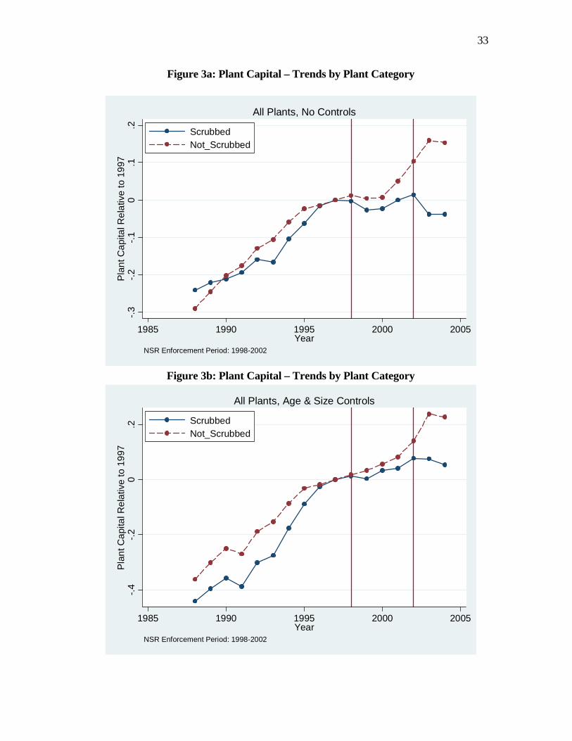
Figures 3a-c and 4a-c plot Not Scrubbedi ∗ κt and Scrubbedi ∗ κt (1997 is the omitted year).
Consider first Figure 3a, based on specifications with ln(Total Capital) as the dependent variable
where we do not estimate Largei ∗ κt or Y oungi ∗ κt, the year-effects by size and age group. In
the years before 1998, the beginning of the treatment period, the trends in input use are not the
same: Scrubbed plants’ capital stocks grow more slowly than Not Scrubbed plants. This causes
two problems. First, this suggests that the two groups of plants trend at different rates, which
could suggest that the Scrubbed plants may not be good controls during the treatment period, if
the difference in trends continues. Second, even if the Scrubbed and Not Scrubbed plants followed
similar trends during the treatment phase (absent an NSR effect), the pre-period mean will be
lower for the Not Scrubbed plants, which will cause the difference-in-difference methodology to
estimate a larger change for these plants.
Figure 3b plots Not Scrubbedi ∗ κt and Scrubbedi ∗ κt from specifications that included the
age- and size-specific year effects, Largei ∗ κt and Y oungi ∗ κt. In this specification, Scrubbed
plants’ capital appear to grow more quickly than Not Scrubbed.
As we document above, installing scrubbers entails a large capital expenditure. If some
of the Scrubbed plants in Figure 3b installed their equipment during the pre-period, this could
explain why their capital was growing faster than Not Scrubbed plants. Figure 3c plots coefficient
16Note that this equation replicates equation (8), our main estimating equation, but captures the treatmenteffects through the NotScrubbed year effects.
18
estimates from the same specification depicted in Figure 3b, but estimated on the subset of plants
that either had no scrubber or for which we could confirm that the scrubber was installed before
the data set begins (before 1988). We have scrubber installation dates for only approximately
80 percent of our plants, so the restriction may exclude plants with scrubbers built before the
period covered by our data.17
In Figure 3c, the Scrubbed and Not Scrubbed plants appear to follow very similar trends in
capital during the pre-period. The year effects during the treatment period suggest that there
was an NSR effect and that Scrubbed plants reduced capital spending relative to Not Scrubbed
plants. The next section reports regression estimates to test this hypothesis directly. Based on
the pre-period trends, we will focus on results that include age- and size-specific year effects and
that exclude plants at which scrubbers were installed after 1988.
Figures 4a-c depict the year effects for Scrubbed and Not Scrubbed plants from specifications
with ln(Total O&M) as the dependent variable. In Figure 4a, the newer, scrubbed plants appear
to increase their rate of expenditures on O&M slightly faster than the older plants, which may
have already been at higher annual O&M expenditure levels. When we control for age- and
size-specific trends in Figure 4b the difference diminishes. When we exclude plants that might
have installed scrubbers during the pre-period, the Scrubbed plants appear to spend on O&M
at an increasing rate relative to Not Scrubbed plants, although the differences are statistically
different in only three of the ten pre-period years.
The data that we use to estimate equation (8) for fuel and emissions is only available begin-
ning in 1996, so we have a very short (two-year) pre-period. Our plant-level database contains
information on heatrates beginning in 1988, and we have produced figures similar to 3a-c and 4a-c
using ln(HeatRate) as the dependent variable. In all specifications, the trends in ln(HeatRate)
were similar across Scrubbed and Not Scrubbed plants, and in no case could we reject the hy-
17Note that this restriction requires that the plant itself was built before 1988. We have not imposed a similarrequirement on the nonscrubbed plant, although results are almost identical when we do as there was only onenonscrubbed plant built after 1988. Once we exclude plants for which scrubber installation was either unknownor after 1987, we have 20 Small and 22 Large plants that are Scrubbed and 33 Y oung and 9 Old plants that areScrubbed.
19
pothesis that the year effects were the same across the two groups of plants. This provides some
comfort that trends in Scrubbed and Not Scrubbed heat rates were similar, although the result
should be interpreted cautiously, both because it is estimated at the plant- and not the unit-level
and because the plant-level heat rate data can be noisy.
The second approach we take to controlling for pre-period differences in input use trends is
to condition on the trends directly by estimating versions of the following equation:
for input I at plant i in year τ . We estimate separate versions of equation (10) for τ ∈
{1998, 1999, ...2004}. We expect β2 to follow the same pattern as in equation (8): negative for
I ∈ {capital} in 1998-2002 if the heightened enforcement of NSR caused utilities to cut back
on investing in plants that were at risk of triggering expensive upgrades in pollution control
equipment (Not Scrubbed plants), but positive for I ∈ {fuel} for Tau ∈ {1998 − 2002} if low
capital investment caused fuel efficiency to degrade. Any post-enforcement catch-up would be
reflected in positive values of β2 in 2003 and 2004. As in equation (8), Q measures electrical
output and Xiτ is a vector of contemporaneous control variables. Pi is a vector that includes levels
of input use and, in some specifications, output (Q) from the years before the NSR enforcement
period began. This approach is very similar to one used by Greenstone (2004). Essentially,
the variable Pi controls flexibly for the pre-existing trends in input use, and β2 is identified by
differences between Scrubbed andNot Scrubbed plants in the NSR enforcement period conditional
on these trends.
Potential Endogeneity of Output Levels
One further issue we confront in estimating factor demand equations as in (8) is the potential
for simultaneity in the relationship between Q and I. This would arise if units adjusted their
output to accommodate shocks to their efficiency, for example lowering output when a malfunc-
tioning piece of equipment causes the unit to be less fuel efficient. This is analogous to the
20
simultaneity of inputs problem identified in much of the production function literature.18 We
choose to address the simultaneity problem by instrumenting for Q with electricity demand at
the state level. This instrument is highly correlated with unit-level output but uncorrelated with
information that an individual plant manager has about a particular unit’s shock to productiv-
ity. We do not instrument for Q when we estimate equation (10). Under the assumption that
capital investment in previous periods measures the plant-specific productivity shock (this is the
assumption used by Olley and Pakes (1996)), εiτ will not be correlated with Q.
4 Empirical Results
This section presents the results from estimating equations (8) and (10). Because the data sets
and control variables differ across nonfuel and fuel inputs, we consider the two sets of results
separately.
4.1 Capital and Operations and Maintenance Inputs
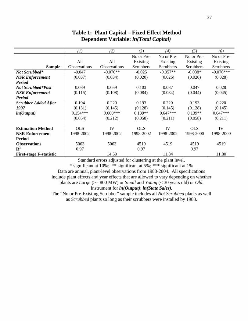
Table 1 reports results from estimating equation (8) using ln(Total Capital) as the dependent
variable. In light of the analysis in the previous section, all specifications include plant-fixed
effects. We also estimate every specification with year-fixed effects that vary for big and small
plants and old and young plants. In column (1), which includes all of the plants in the dataset
and is estimated using OLS, the coefficient on Not Scrubbed ∗ NSR Enforcement Period is
negative, suggesting that plants that were concerned about NSR reduced capital investment
relative to control plants during the period of heightened NSR enforcement. The coefficient is
statistically indistinguishable from zero.
The specification reported in column (2) is nearly identical to column (1), except that we
use ln(StateSales) as the instrument for ln(Output). The coefficient on ln(StateSales) in the
first-stage regression is positive, since higher demand in a year (e.g. due to hotter weather) causes
18See Griliches and Mairesse (1998) for an overview of the issue and survey of various approaches to dealingwith it. Recent papers by Olley and Pakes (1996) and Levinsohn and Petrin (2003) propose structural approachesto addressing simultaneity. Ackerberg, Caves and Frazer (2005) compares and critiques the approaches proposedby them. Fabrizio, Rose and Wolfram (2007) address the simultaneity problem by instrumenting.
21
plants to run more intensively over the year. The F-statistic soundly rejects the hypothesis that
the coefficient is zero (F=14.59), suggesting that our instrument is not weak a la Staiger and
Stock (1997).19 Note that the coefficient on ln(Output) increases substantially between the OLS
and IV specifications. This is consistent with a negative correlation between input shocks and
output. Purely mechanically, plants must be shut down and the boilers cold for most capital
projects to proceed. Also, since our data are measured yearly, this could reflect the fact that plant
outages due to capital equipment failure necessitate large capital expenditures in the following
months.
When we instrument for output, the coefficient on Not Scrubbed∗NSR Enforcement Period
increases in absolute value. Output at Not Scrubbed plants increased during the treatment period
(this could be independent of the enforcement and driven by the demand shocks captured in our
instrument), so with a larger coefficient on output suggesting a tighter relationship between out-
put and capital, the effects of the reduced capital during the NSR period are accentuated. Also,
the standard error goes down slightly, so the negative coefficient is now statistically significant
at the five percent level.
Figure 3c above suggested that capital levels at Scrubbed and Not Scrubbed plants tracked
each other most closely once we excluded plants that could have been installing scrubbers
during the pre-period (1988-1997). Columns (3) and (4) report OLS and IV results on this
subset of the data. Comparable to columns (1) and (2), the coefficients on Not Scrubbed ∗
NSR Enforcement Period are both negative, and larger and statistically significant in the IV
specification.
Finally, columns (5) and (6) report specifications where the NSR enforcement period ends
in 2000. It is possible that utilities were confident that a Bush Administration would interpret
NSR less strictly and did not need the detailed policy statement in the Equipment Replacement
Provision to signal that the cost of investing in their Not Scrubbed plants had again fallen.
Consistent with this hypothesis, the coefficients on Not Scrubbed ∗NSR Enforcement Period
19F-statistics from the other IV specifications are reported in the final row of the table. They are also bothabove 11.5.
22
in columns (5) and (6) are larger in absolute value than the comparable coefficients in columns
(3) and (4).
The magnitude of the coefficient in column (6) suggests that plants concerned about triggering
NSR reduced Total Capital by over seven percent relative to the control plants during the
period when NSR enforcement was most likely. Given that Total Capital measures capital
stock, this amounts to a substantial change in annual expenditures. For example, at the mean
level of Total Capital for Not Scrubbed plants, a seven percent reduction reflects approximately
a $25 million dollar reduction in total capital. Consistent with this finding, when we estimate a
specification idential to column (6) but use the change in Total Capital interacted with a dummy
variable for positive changes, the coefficient on Not Scrubbed ∗ NSR Enforcement Period (-
0.824, standard error = 0.196) suggests a reduction of over 50 percent.
In all columns of Table 1, we include two additional control variables. Not Scrubbed ∗
Post NSR Enforcement Period tests whether utilities changed their investment patterns at
Not Scrubbed plants after the heightened enforcement of NSR. The positive coefficient is con-
sistent with a policy of accelerating investments to “make up” for the period of low investment,
though the standard errors on the coefficient are large and it is never statistically distinguishable
from zero. Finally, the coefficient on Scrubber Added After 1997 suggests that plants increase
their capital by around 20 percent when they add scrubbers, though it is also estimated with
considerable noise and statistically indistinguishable from zero.
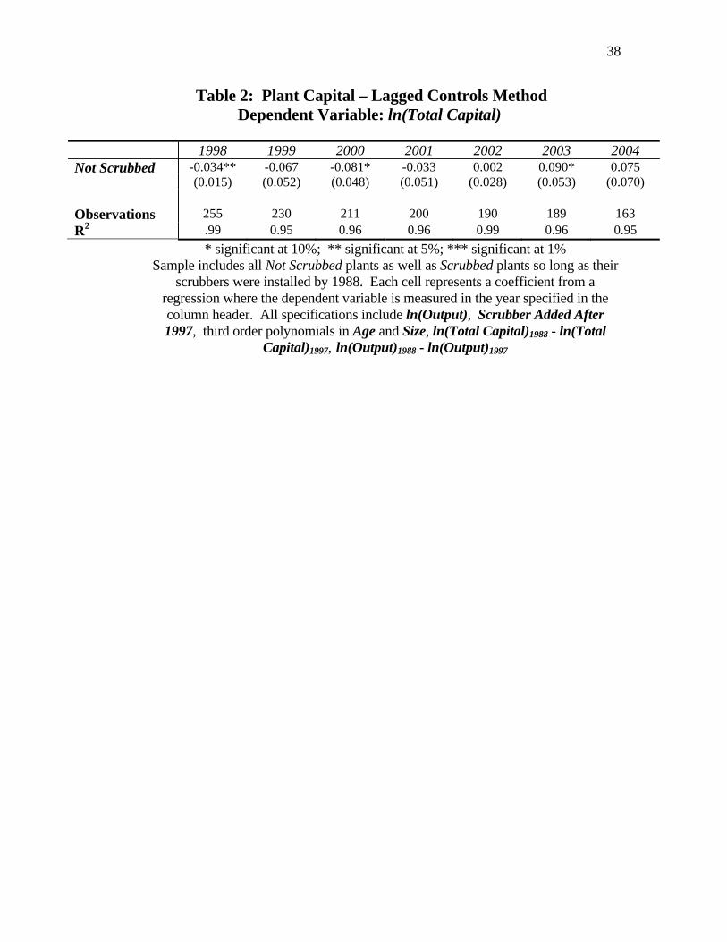
Table 2 reports estimates of equation (10) using ln(Total Capital) levels in 1998 to 2004. The
table is based on the same sample as reported in columns (3)-(6) of Table 1 (i.e., excluding plants
that installed scrubbers after 1988). The signs of the coefficient estimates are consistent with
those reported in Table 1, suggesting slower growth in capital at Not Scrubbed plants in the 1998-
2002 period. The implied magnitudes of the effects, eight percent less capital at Not Scrubbed
plants in 2000 and more than three percent in 1998, imply a slightly larger effect than reflected
in Table 1.20 Not Scrubbed plants invested significantly more capital in 2003, perhaps suggesting
20In light of the differences in age and capacity identified in Section 3, we re-estimated the specifications reported
23
they were making up for several years of low investment.
As the number of observations by year reported in Table 2 indicates, we have a fair amount of
attrition in our data set. This is primarily due to divestitures, wherein plants are transferred to
nonutility owners who are no longer required to report plant financial statistics to the regulatory
agencies. Between 1998 and 2004, there were only 25 coal units retired (out of over 800 in our data
set) and 8 coal plants retired (out of over 300 in our data set). As a result, it seems unlikely that
the attrition is related to efficiency.21 We estimated versions of both the specifications reported
in the fifth column of Table 1 and the specifications reported in Table 2 using a balanced panel
and obtained similar results to those reported.
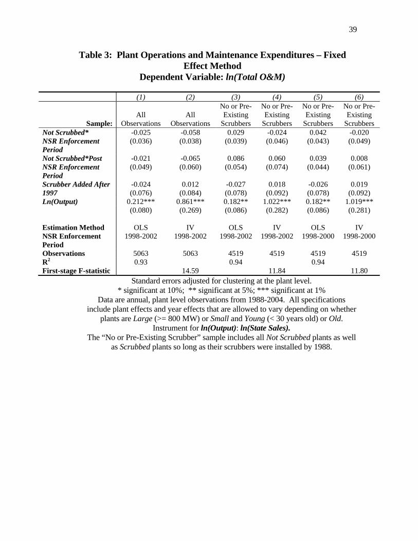
Table 3 report specifications of equation (8) for the operations and maintenance expenditures.
The coefficients on Not Scrubbed ∗ NSR Enforcement Period are small and statistically in-
distinguishable from zero across all specifications. Specifications based on equation (10) showed
similarly inconclusive results in the early years or the treatment period, and significantly negative
results in 2001 and 2002.
The results discussed in this section suggest that the increased enforcement of NSR during
the 1998-2002 period may have reduced capital spending at plants at risk of triggering a costly
review. NSR enforcement does not seem to have systematically reduced spending on O&M.
4.2 Fuel Efficiency and Emissions
The data we use to estimate equation (8) for fuel inputs are available with much finer disag-
gregation than the capital and O&M expenditures both over time and across units, but are
unfortunately only available beginning in 1996. As described more fully in the appendix, the
fuel input data are collected by the EPA every hour from each unit. Since we have nearly 900
units operating over 9 years, we begin with an hourly data set with over 55 million observations.
in Table 2 using five-part linear splines in both Age and Size instead of the third-order polynomial. The resultswere very similar to those reported.
21Divestitures were essentially mandated by some state regulatory agencies as part of the electricity industryrestructuring. See Bushnell and Wolfram (2005).
24
The NSR effects that we are looking for require nowhere near this level of detail, but the con-
trol variables that we use, output and temperature, vary hour to hour in important ways. To
balance these factors, we aggregated observations for each unit up to the weekly level.22 Since
the temperature data are only available after July 1996, we do not use the first half of 1996
in our specifications, although unreported specifications that omitted temperature and included
observations from the first half of 1996 were very similar to the reported results.
Table 4 reports specifications for which the dependent variable is ln(HeatRate). All speci-
fications include unit-fixed effects and year-fixed effects that vary depending on whether a unit
is Large or Small and depending on whether it is Y oung or Old. The specification in column
(1) is based on all units in the data set and uses 1998-2002 as the treatment period, while col-
umn (2) is estimated using all non-scrubbed units and scrubbed units if their scrubbers were
intsalled before 1988. Column (3), which is based on the same data sample as column (2),
uses 1998-2000 as the treatment period, and column (4) uses instrumental variables to estimate
a similar specification to column (3).23 Note that in the case of fuel efficiency, instrument-
ing has the classic effect and dampens its relationship with output. The variable of interest,
Not Scrubbed∗NSR Enforcement Period, is small and statistically indistinguishable from zero
in all specifications. The coefficient is so precisely estimated that we can reject the hypothesis
that Not Scrubbed units’ heat rates increased (i.e., fuel efficiency decreased) by one percent in
every specification.
Table 5 reports results that evaluate whether emissions rates changed with heightened NSR
enforcement. The first two columns of Table 5 are estimated using ln(NOxRate) as the dependent
variable, and the last two columns use ln(SO2Rate) as the dependent variable. Sulfur dioxide
(SO2) and nitrogen oxide (NOx) are the most expensive pollutants for coal-fired power plants to
22In related work, we used the hourly data to estimate a nonparametric relationship between output and fuelefficiency (Bushnell and Wolfram, 2005). The estimated relationship is quite close to the log-log specification weuse here.
23To save space, Table 4 does not include IV versions of the specifications in columns (1) and (2). In thosespecifications, the coefficients on Not Scrubbed ∗NSR Enforcement Period is smaller in absolute value than incolumn (4). Also, hourly sales data were not available for 6 states in 2004, so there are slightly fewer observationsin column (4) than in column (3). OLS results using the column (4) data set were very similar to those reportedin column (3).
25
mitigate.24 The specifications are comparable to columns (3) and (4) of Table 4.25 Results from
other specifications, including those comparable to columns (1) through (4) of Tables 1 and 3,
similarly showed no discernible effect. The specifications in all of the columns of Table 5 suggest
that increased NSR enforcement had no appreciable effect on either NOx or SO2 emissions.26
As noted above, a feared perverse outcome is that rigorous enforcement of NSR inhibited
firms from investing in capital leading to higher emissions from existing plants than there would
be if they were not policed. Our results are inconsistent with this outcome, at least over the short
time period when NSR was strictly enforced. Note that our specifications test whether emissions
at grandfathered plants are higher under rigorous enforcement of NSR than they would have
been under a lax enforcement regime. It is theoretically possible that an increase in emissions
from existing plants subject to tight NSR enforcement could more than offset the reduction in
emissions from the new plants driven by their compliance with the New Source Performance
Standards, suggesting that emissions are overall higher with the regulation than they would be
absent any regulation. As we find no discernible impact on emissions at the existing plants, we
do not consider this counterfactual.
5 Conclusion
This paper considers the effects of NSR on coal-fired power plant operations. A vintage-differentiated
regulation such as NSR can distort behavior in several ways. Perhaps most obviously, it may
cause owners of existing plants to keep their capital in service for longer since building a new
24Carbon dioxide was not mitigated during our sample period, and CO2 emissions are proportional to fuelefficiency.
25The results in Table 5 include three dummy variables to control for changes in regional regulations thatimpacted NOx emissions rates, including the Ozone Transport Commission NOx Budget Program and the NOxBudget Trading Program. While highly significant, the inclusion of the dummy variables does not affect thecoefficients on Not Scrubbed ∗ NSR Enforcement Period, suggesting that there are roughly equal fractions ofscrubbed and unscrubbed plants across the regions affected and not affected by these regulations.
26Keohane, Mansur and Voynov (2009) find that plants that faced a high probability of being sued reduced SO2emissions in 1999. That paper has a different control group than ours – plants that faced a low probability of beingsued, whether or not they had a scrubber. They also have a different specification for the emissions regression, asthey estimate emissions while our dependent variable is the emissions rate. Also, we control flexibly for differentialtrends by age and size of the plant. However, we suspect that the main cause of the differences is that Keohane,Mansur and Voynov (2009) consider the addition of a scrubber, if the investment happened during the treatmentwindow, as a treatment effect. By contrast, we isolate plants that add scrubbers during the treatment windowwith a separate dummy variable. For this set of plants, emissions do indeed decline substantially.
26
plant becomes more expensive. Early work on NSR found some evidence of this effect (Maloney
and Brady, 1988 and Nelson, Tietenberg and Donihue, 1993). At the same time, monitoring of
existing plants to ensure that significant, life-extending upgrades include state-of-the-art pollu-
tion control equipment may cause firms to invest less in their plants. We find some evidence
that this effect was relevant at coal-fired power plants, but no evidence that this led to reduced
fuel efficiency or increased emissions. There are several possible interpretations of this result. It
could imply that industry claims about the efficiency impacts of heightened enforcement were
overblown, or even that the new bias against capital introduced by NSR offset some pre-existing
bias in favor of capital.27 However, given the complexities and durable nature of power plants, it
is also possible that continued under-investment in the capital stock would have eventually led
to a decline in fuel efficiency. We find some evidence that the reductions in capital investment
during this period were offset when the rules were subsequently relaxed.
Over the past decade, the New Source Review program has come under fire from both en-
vironmentalists and the utility companies. The environmentalists, apparently frustrated that
plants exempt from regulations in the 1970s are still in service today, contend that utilities are
routinely flouting the regulations and performing major overhauls to their plants without apply-
ing for permits. While this might be true, it is possible that the utilities would have overhauled
their plants even in the absence of the regulations, so the question boils down to how stringently
the EPA should enforce the NSR requirement and whether the old units should be required to
install pollution control equipment.
Since the early 1990’s the EPA has moved away from command-and-control regulation and has
implemented or proposed implementing market-based cap-and-trade programs. This calls into
question the role of performance standards such as NSR. For instance, the Acid Rain Program
caps the number of SO2 permits available nationwide, so if the EPA took steps to require the
older plants to install scrubbers, this would just mean that those plants could sell their permits
27For example, if plant owners were allowed a regulatory rate-of-return in excess of their true cost of capital, the“Averch-Johnson effect” may have led toward excessive spending on capital. The additional capital cost introducedby the NSR effect may then have offset this pro-investment bias and pushed the plant closer to an efficient frontier.
27
and other plants could increase their emissions of SO2. In light of this shift, EPA regulators
with whom we have spoken suggest that NSR is now most effective as a tool for preventing local
“hot spots” of pollution. With performance standards for greenhouse gas emissions potentially
on the horizon, there will again be questions about the extent to which new source performance
standards should be imposed on existing plants that retrofit. This paper provides evidence that
applying these standards can induce distortions in capital investment.
28
References
[1] Ackerberg, Dan, Kevin Caves and Garth Frazer (2005). “Structural Identification of Pro-
duction Functions,” UCLA mimeo.
[2] Buckheit, Bruce (2004). Former EPA Enforcement Chief. Personal testimony. Sen-
ate Democratic Policy Committee Hearing. February 6. ”Clearing the Air: An
Oversight Hearing on the Administration’s Clean Air Enforcement Program.”
http://democrats.senate.gov/dpc/dpc-hearing.cfm?A=11 (Last accessed January 2008.)
[3] Bushnell, James and Catherine Wolfram (2005). “Ownership Change, Incentives and Plant
Efficiency: The Divestiture of U.S. Electric Generation Plants.” CSEM Working Paper WP-
140, University of California Energy Institute. March. Available at www.ucei.org.
[4] Christensen, Laurits R. and William H. Greene (1976). “Economies of Scale in U.S. Electric
Power Generation,” Journal of Political Economy, 84 (4), 655-676.
[5] Cusick, Daniel (2007). “AEP Settlement Ends Long Battle over Power Plant Upgrades,”
Standard errors adjusted for clustering at the plant level. * significant at 10%; ** significant at 5%; *** significant at 1%
Data are annual, plant-level observations from 1988-2004. All specifications include plant effects and year effects that are allowed to vary depending on whether
plants are Large (>= 800 MW) or Small and Young (< 30 years old) or Old. Instrument for ln(Output): ln(State Sales).
The “No or Pre-Existing Scrubber” sample includes all Not Scrubbed plants as well as Scrubbed plants so long as their scrubbers were installed by 1988.
* significant at 10%; ** significant at 5%; *** significant at 1% Sample includes all Not Scrubbed plants as well as Scrubbed plants so long as their
scrubbers were installed by 1988. Each cell represents a coefficient from a regression where the dependent variable is measured in the year specified in the column header. All specifications include ln(Output), Scrubber Added After 1997, third order polynomials in Age and Size, ln(Total Capital)1988 - ln(Total
Standard errors adjusted for clustering at the plant level. * significant at 10%; ** significant at 5%; *** significant at 1%
Data are annual, plant level observations from 1988-2004. All specifications include plant effects and year effects that are allowed to vary depending on whether
plants are Large (>= 800 MW) or Small and Young (< 30 years old) or Old. Instrument for ln(Output): ln(State Sales).
The “No or Pre-Existing Scrubber” sample includes all Not Scrubbed plants as well as Scrubbed plants so long as their scrubbers were installed by 1988.
Standard errors adjusted for clustering at the unit level. * significant at 10%; ** significant at 5%; *** significant at 1%
Data are weekly, unit level observations from July 1996-December 2004. All specifications include unit effects and year effects that are allowed to vary
depending on whether units are Large (>= 400 MW) or Small and Young (< 30 years old) or Old. Instrument for ln(Output): ln(State Sales).
The “No or Pre-Existing Scrubber” sample includes all Not Scrubbed units as well as Scrubbed units so long as their scrubbers were installed by 1988.
Temperature -0.157*** -0.161*** -0.006 -0.006 (0.013) (0.014) (0.009) (0.010)
Estimation Method OLS IV OLS IV NSR Enforcement Period 1998-2000 1998-2000 1998-2000 1998-2000 Observations 308,952 306,328 311,965 309,339 R2 0.66 0.84 First-stage F-statistic 218.3 217.7
Standard errors adjusted for clustering at the unit level. * significant at 10%; ** significant at 5%; *** significant at 1%
Data are weekly, unit level observations from July 1996-December 2004. All specifications also include a dummy variable indicating the beginning of the Ozone Transport Commission NOx Budget Program, which covered 9 states and DC and
began in 1999, and two dummy variables indicating the beginning of the NOx Budget Trading Program in 2004—one variable for the units in the states that were already part of the Ozone Transport Commission and a second for the units in the
12 states newly covered by the NOx Budget Trading Program. All specifications include unit effects and year effects that are allowed to vary depending on whether units are Large (>= 400 MW) or Small and Young (< 30
years old) or Old. Instrument for ln(Output): ln(State Sales). All specifications are estimated using the “No or Pre-Existing Scrubber” sample, which includes all Not Scrubbed units as well as Scrubbed units so long as their