Error analysis of the s-step Lanczos method in finite ... · ERROR ANALYSIS OF THE S-STEP LANCZOS...

Error analysis of the s-step Lanczos method in finite

precision

Erin CarsonJames Demmel

Electrical Engineering and Computer SciencesUniversity of California at Berkeley

Technical Report No. UCB/EECS-2014-55

http://www.eecs.berkeley.edu/Pubs/TechRpts/2014/EECS-2014-55.html

May 6, 2014

Copyright © 2014, by the author(s).All rights reserved.

Permission to make digital or hard copies of all or part of this work forpersonal or classroom use is granted without fee provided that copies arenot made or distributed for profit or commercial advantage and that copiesbear this notice and the full citation on the first page. To copy otherwise, torepublish, to post on servers or to redistribute to lists, requires prior specificpermission.

Acknowledgement

Research is supported by DOE grants DE-SC0004938, DE-SC0005136,DE-SC0003959, DE-SC0008700, DE-FC02-06-ER25786, and AC02-05CH11231, DARPA grant HR0011-12-2-0016, as well as contributionsfrom Intel, Oracle, and MathWorks.

ERROR ANALYSIS OF THE S-STEP LANCZOS METHOD INFINITE PRECISION

ERIN CARSON AND JAMES DEMMEL

Abstract. The s-step Lanczos method is an attractive alternative to the classical Lanczosmethod as it enables an O(s) reduction in data movement over a fixed number of iterations. Thiscan significantly improve performance on modern computers. In order for s-step methods to be widelyadopted, it is important to better understand their error properties. Although the s-step Lanczosmethod is equivalent to the classical Lanczos method in exact arithmetic, empirical observationsdemonstrate that it can behave quite differently in finite precision. In the s-step Lanczos method,the computed Lanczos vectors can lose orthogonality at a much quicker rate than the classical method,a property which seems to worsen with increasing s.

In this paper, we present, for the first time, a complete rounding error analysis of the s-stepLanczos method. Our methodology is analogous to Paige’s rounding error analysis for the classicalLanczos method [IMA J. Appl. Math., 18(3):341–349, 1976]. Our analysis gives upper bounds on theloss of normality of and orthogonality between the computed Lanczos vectors, as well as a recurrencefor the loss of orthogonality. The derived bounds are very similar to those of Paige for classicalLanczos, but with the addition of an amplification term which depends on the condition numberof the Krylov bases computed every s-steps. Our results confirm theoretically what is well-knownempirically: the conditioning of the Krylov bases plays a large role in determining finite precisionbehavior.

Key words. Krylov subspace methods, error analysis, finite precision, roundoff, Lanczos, avoid-ing communication, orthogonal bases

AMS subject classifications. 65G50, 65F10, 65F15, 65N15, 65N12

1. Introduction. Given an n-by-n symmetric matrix A and a starting vector v0with unit 2-norm, m steps of the Lanczos method [21] theoretically produces the or-thonormal matrix Vm = [v0, . . . , vm] and the (m+1)-by-(m+1) symmetric tridiagonalmatrix Tm such that

AVm = VmTm + βm+1vm+1eTm+1. (1.1)

When m = n − 1, the eigenvalues Tn−1 are the eigenvalues of A. In practice, theeigenvalues of T are still good approximations to the eigenvalues of A when m� n−1,which makes the Lanczos method attractive as an iterative procedure. Many Krylovsubspace methods (KSMs), including those for solving linear systems and least squaresproblems, are based on the Lanczos method. In turn, these various Lanczos-basedmethods are the core components in numerous scientific applications.

Classical implementations of Krylov methods, the Lanczos method included, re-quire one or more sparse matrix-vector multiplications (SpMVs) and one or moreinner product operations in each iteration. These computational kernels are bothcommunication-bound on modern computer architectures. To perform an SpMV,each processor must communicate entries of the source vector it owns to other pro-cessors in the parallel algorithm, and in the sequential algorithm the matrix A mustbe read from slow memory. Inner products involve a global reduction in the paral-lel algorithm, and a number of reads and writes to slow memory in the sequentialalgorithm (depending on the size of the vectors and the size of the fast memory).

Thus, many efforts have focused on communication-avoiding Krylov subspacemethods (CA-KSMs), or s-step Krylov methods, which can perform s iterations withO(s) less communication than classical KSMs; see, e.g., [4, 5, 7, 9, 10, 16, 17, 8, 33, 35].In practice, this can translate into significant speedups for many problems [24].

1

2 ERIN CARSON AND JAMES DEMMEL

Equally important to the performance of each iteration is the convergence rate ofthe method, i.e., the total number of iterations required until the desired convergencecriterion is met. Although theoretically the Lanczos process described by (1.1) pro-duces an orthogonal basis and a tridiagonal matrix similar to A after n steps, theseproperties need not hold in finite precision. The effects of roundoff error on the idealLanczos process were known to Lanczos when he published his algorithm in 1950.Since then, much research has been devoted to better understanding this behavior,and to devise more robust and stable algorithms.

Although s-step Krylov methods are mathematically equivalent to their classicalcounterparts in exact arithmetic, it perhaps comes as no surprise that their finiteprecision behavior may differ significantly, and that the theories developed for classicalmethods in finite precision do not hold for the s-step case. It has been empiricallyobserved that the behavior of s-step Krylov methods deviates further from that ofthe classical method as s increases, and that the severity of this deviation is heavilyinfluenced by the polynomials used for the s-step Krylov bases (see, e.g., [1, 4, 17, 18]).

Arguably the most revolutionary work in the finite precision analysis of classicalLanczos was a series of papers published by Paige [25, 26, 27, 28]. Paige’s analysissuccinctly describes how rounding errors propagate through the algorithm to impedeorthogonality. These results were developed to give theorems which link the loss oforthogonality to convergence of the computed eigenvalues [28]. No analogous theorycurrently exists for the s-step Lanczos method.

In this paper, we present, for the first time, a complete rounding error analysisof the s-step Lanczos method. Our analysis here for s-step Lanczos closely followsPaige’s rounding error analysis for orthogonality in classical Lanczos [27].

We present upper bounds on the normality of and orthogonality between thecomputed Lanczos vectors, as well as a recurrence for the loss of orthogonality. Thederived bounds are very similar to those of Paige for classical Lanczos, but withthe addition of an amplification term which depends on the condition number ofthe Krylov bases computed every s steps. Our results confirm theoretically whatis well-known empirically: the conditioning of the Krylov bases plays a large role indetermining finite precision behavior. In particular, if one can guarantee that the basiscondition number is not too large throughout the iteration, the loss of orthogonalityin the s-step Lanczos method should not be too much worse than in classical Lanczos.As Paige’s subsequent groundbreaking convergence analysis [28] was based largely onthe results in [27], our analysis here similarly serves as a stepping stone to furtherunderstanding of the s-step Lanczos method.

The remainder of this paper is outlined as follows. In Section 2, we presentrelated work in s-step Krylov methods and the analysis of finite precision Lanczos. InSection 3, we review a variant of the Lanczos method and derive the correspondings-step Lanczos method, as well as provide a numerical example that will help motivateour analysis. In Section 4, we first state our main result in Theorem 4.2 and commenton its interpretation; the rest of the section is devoted to its proof. In Section 5,we recall our numerical example from Section 3 in order to demonstrate the boundsproved in Section 4. Section 6 concludes with a discussion of future work.

2. Related work. We briefly review related work in s-step Krylov methods aswell as work related to the analysis of classical Krylov methods in finite precision.

2.1. s-step Krylov subspace methods. The term ‘s-step Krylov method’,first used by Chronopoulos and Gear [6], describes variants of Krylov methods wherethe iteration loop is split into blocks of s iterations. Since the Krylov subspaces

ERROR ANALYSIS OF S-STEP LANCZOS 3

required to perform s iterations of updates are known, bases for these subspaces canbe computed upfront, inner products between basis vectors can be computed with oneblock inner product, and then s iterations are performed by updating the coordinatesin the generated Krylov bases (see Section 3 for details). Many formulations andvariations have been derived over the past few decades with various motivations,namely increasing parallelism (e.g., [6, 35, 36]) and avoiding data movement, bothbetween levels of the memory hierarchy in sequential methods and between processorsin parallel methods. A thorough treatment of related work can be found in [17].

Many empirical studies of s-step Krylov methods found that convergence oftendeteriorated using s > 5 due to the inherent instability of the monomial basis. Thismotivated research into the use of better-conditioned bases (e.g., Newton or Cheby-shev polynomials) for the Krylov subspace, which allowed convergence for higher svalues (see, e.g., [1, 16, 18, 31]). Hoemmen has used a novel matrix equilibration andbalancing approach to achieve similar effects [17].

The term ‘communication-avoiding Krylov methods’ refers to s-step Krylov meth-ods and implementations which aim to improve performance by asymptotically de-creasing communication costs, possibly both in computing inner products and comput-ing the s-step bases, for both sequential and parallel algorithms; see [9, 17]. Hoemmenet al. [17, 24] derived communication-avoiding variants of Lanczos, Arnoldi, ConjugateGradient (CG) and the Generalized Minimum Residual Method (GMRES). Details ofnonsymmetric Lanczos-based CA-KSMs, including communication-avoiding versionsof Biconjugate Gradient (BICG) and Stabilized Biconjugate Gradient (BICGSTAB)can be found in [4]. Although potential performance improvement is our primarymotivation for studying these methods, we use the general term ‘s-step methods’ hereas our error analysis is independent of performance.

Many efforts have been devoted specifically to the s-step Lanczos method. Thefirst s-step Lanczos methods known in the literature are due to Kim and Chronopou-los, who derived a three-term symmetric s-step Lanczos method [19] as well as athree-term nonsymmetric s-step Lanczos method [20]. Hoemmen derived a three-termcommunication-avoiding Lanczos method, CA-Lanczos [17]. Although the three-termvariants require less memory, their numerical accuracy can be worse than implemen-tations which use two coupled two-term recurrences [15]. A two-term communication-avoiding nonsymmetric Lanczos method (called CA-BIOC, based on the ‘BIOC’ ver-sion of nonsymmetric Lanczos of Gutknecht [14]) can be found in [2]. This workincludes the derivation of a new version of the s-step Lanczos method, equivalent inexact arithmetic to the variant used by Paige [27]. It uses a two-term recurrence likeBIOC, but is restricted to the symmetric case and uses a different starting vector.

For s-step KSMs that solve linear systems, increased roundoff error in finite pre-cision can decrease the maximum attainable accuracy of the solution, resulting in aless accurate solution than found by the classical method. A quantitative analysis ofroundoff error in CA-CG and CA-BICG can be found in [3]. Based on the work of [34]for conventional KSMs, we have also explored implicit residual replacement strategiesfor CA-CG and CA-BICG as a method to limit the deviation of true and computedresiduals when high accuracy is required (see [3]).

2.2. Error analysis of the Lanczos method. Lanczos and others recognizedearly on that rounding errors could cause the Lanczos method to deviate from itsideal theoretical behavior. Since then, various efforts have been devoted to analyzing,and explaining, and improving the finite precision Lanczos method.

Widely considered to be the most significant development was the series of pa-


pers by Paige discussed in Section 1. Another important development was due toGreenbaum and Strakos, who performed a backward-like error analysis which showedthat finite precision Lanczos and CG behave very similarly to the exact algorithmsapplied to any of a certain class of larger matrices [12]. Paige has recently showna similar type of augmented stability for the Lanczos process [29]. There are manyother analyses of the behavior of various KSMs in finite precision, including somemore recent results due to Wulling [37] and Zemke [38]; for a thorough overview ofthe literature, see [22, 23].

A number of strategies for maintaining the orthogonality among the Lanczosvectors were inspired by the analysis of Paige, such as selective reorthogonalization [30]and partial reorthogonalization [32]. Recently, Gustafsson et al. have extended suchreorthogonalization strategies for classical Lanczos to the s-step case [13].

3. The s-step Lanczos method. The classical Lanczos method is shown inAlgorithm 1. We use the same variant of Lanczos as used by Paige in his erroranalysis for classical Lanczos [27] to allow easy comparison of results. This is thefirst instance of an s-step version of this particular Lanczos variant; other existings-step Lanczos variants are described in Section 2.1. Note that as in [27] our analysiswill assume no breakdown occurs and thus breakdown conditions are not discussedhere. We now give a derivation of s-step Lanczos, obtained from classical Lanczos inAlgorithm 1.

Algorithm 1 Lanczos

Require: n-by-n real symmetric matrix A and length-n starting vector v0 such that‖v0‖2 = 1

1: u0 = Av02: for m = 0, 1, . . . until convergence do3: αm = vTmum4: wm = um − αmvm5: βm+1 = ‖wm‖26: vm+1 = wm/βm+1

7: um+1 = Avm+1 − βm+1vm8: end for

Suppose we are beginning iteration m = sk where k ∈ N and 0 < s ∈ N. Byinduction on lines 6 and 7 of Algorithm 1, we can write

vsk+j , usk+j ∈ Ks+1(A, vsk) +Ks+1(A, usk) (3.1)

for j ∈ {0, . . . , s}, where Ki(A, x) = span{x,Ax, . . . , Ai−1x} denotes the Krylov sub-space of dimension i of matrix A with respect to vector x. Note that since u0 = Av0,if k = 0 we have

vj , uj ∈ Ks+2(A, v0).

for j ∈ {0, . . . , s}.For k > 0, we then define ‘basis matrix’ Yk = [Vk,Uk], where Vk and Uk are size

n-by-(s + 1) matrices whose columns form bases for Ks+1(A, vsk) and Ks+1(A, usk),respectively. For k = 0, we define Y0 to be a size n-by-(s+ 2) matrix whose columnsform a basis for Ks+2(A, v0). Then by (3.1), we can represent vsk+j and usk+j , forj ∈ {0, . . . , s}, by their coordinates (denoted with primes) in Yk, i.e.,

vsk+j = Ykv′k,j , usk+j = Yku′k,j . (3.2)


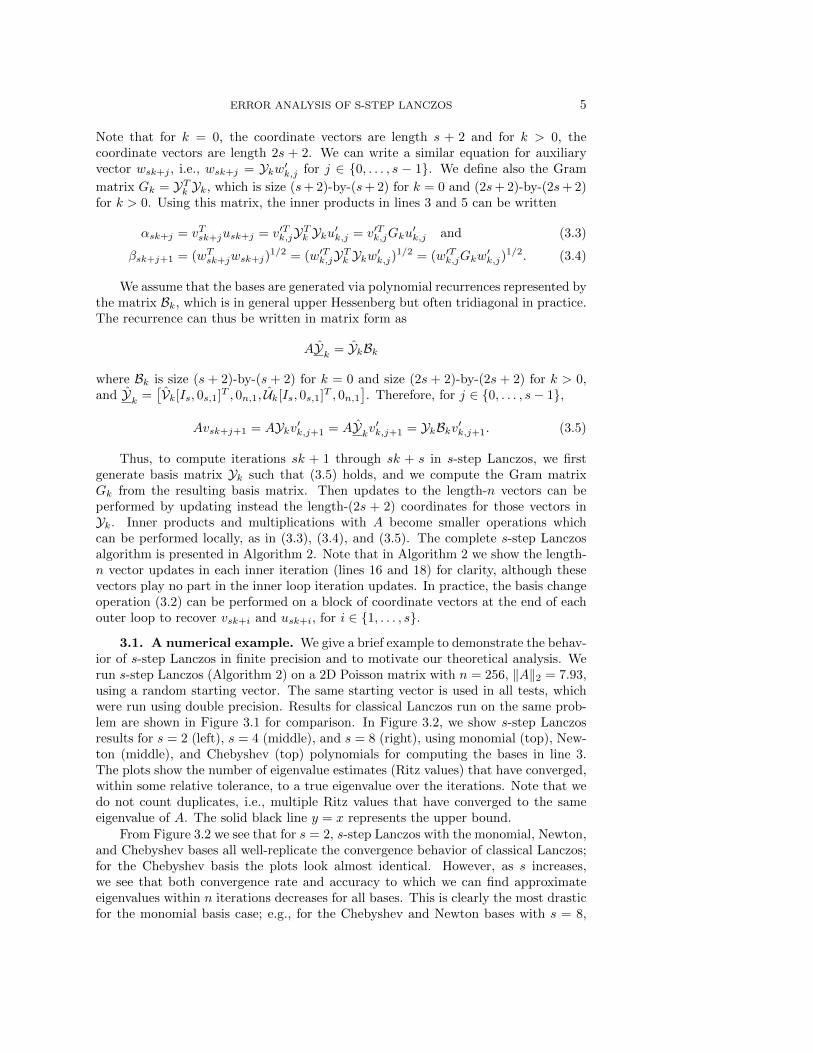
Note that for k = 0, the coordinate vectors are length s + 2 and for k > 0, thecoordinate vectors are length 2s + 2. We can write a similar equation for auxiliaryvector wsk+j , i.e., wsk+j = Ykw′k,j for j ∈ {0, . . . , s − 1}. We define also the Gram

matrix Gk = YTk Yk, which is size (s+ 2)-by-(s+ 2) for k = 0 and (2s+ 2)-by-(2s+ 2)for k > 0. Using this matrix, the inner products in lines 3 and 5 can be written

αsk+j = vTsk+jusk+j = v′Tk,jYTk Yku′k,j = v′Tk,jGku′k,j and (3.3)

βsk+j+1 = (wTsk+jwsk+j)1/2 = (w′Tk,jYTk Ykw′k,j)1/2 = (w′Tk,jGkw

′k,j)

1/2. (3.4)

We assume that the bases are generated via polynomial recurrences represented bythe matrix Bk, which is in general upper Hessenberg but often tridiagonal in practice.The recurrence can thus be written in matrix form as

AYk = YkBk

where Bk is size (s + 2)-by-(s + 2) for k = 0 and size (2s + 2)-by-(2s + 2) for k > 0,and Yk =

[Vk[Is, 0s,1]T , 0n,1, Uk[Is, 0s,1]T , 0n,1

]. Therefore, for j ∈ {0, . . . , s− 1},

Avsk+j+1 = AYkv′k,j+1 = AYkv′k,j+1 = YkBkv′k,j+1. (3.5)

Thus, to compute iterations sk + 1 through sk + s in s-step Lanczos, we firstgenerate basis matrix Yk such that (3.5) holds, and we compute the Gram matrixGk from the resulting basis matrix. Then updates to the length-n vectors can beperformed by updating instead the length-(2s + 2) coordinates for those vectors inYk. Inner products and multiplications with A become smaller operations whichcan be performed locally, as in (3.3), (3.4), and (3.5). The complete s-step Lanczosalgorithm is presented in Algorithm 2. Note that in Algorithm 2 we show the length-n vector updates in each inner iteration (lines 16 and 18) for clarity, although thesevectors play no part in the inner loop iteration updates. In practice, the basis changeoperation (3.2) can be performed on a block of coordinate vectors at the end of eachouter loop to recover vsk+i and usk+i, for i ∈ {1, . . . , s}.

3.1. A numerical example. We give a brief example to demonstrate the behav-ior of s-step Lanczos in finite precision and to motivate our theoretical analysis. Werun s-step Lanczos (Algorithm 2) on a 2D Poisson matrix with n = 256, ‖A‖2 = 7.93,using a random starting vector. The same starting vector is used in all tests, whichwere run using double precision. Results for classical Lanczos run on the same prob-lem are shown in Figure 3.1 for comparison. In Figure 3.2, we show s-step Lanczosresults for s = 2 (left), s = 4 (middle), and s = 8 (right), using monomial (top), New-ton (middle), and Chebyshev (top) polynomials for computing the bases in line 3.The plots show the number of eigenvalue estimates (Ritz values) that have converged,within some relative tolerance, to a true eigenvalue over the iterations. Note that wedo not count duplicates, i.e., multiple Ritz values that have converged to the sameeigenvalue of A. The solid black line y = x represents the upper bound.

From Figure 3.2 we see that for s = 2, s-step Lanczos with the monomial, Newton,and Chebyshev bases all well-replicate the convergence behavior of classical Lanczos;for the Chebyshev basis the plots look almost identical. However, as s increases,we see that both convergence rate and accuracy to which we can find approximateeigenvalues within n iterations decreases for all bases. This is clearly the most drasticfor the monomial basis case; e.g., for the Chebyshev and Newton bases with s = 8,


Algorithm 2 s-step Lanczos

Require: n-by-n real symmetric matrix A and length-n starting vector v0 such that‖v0‖2 = 1

1: u0 = Av02: for k = 0, 1, . . . until convergence do3: Compute Yk with change of basis matrix Bk4: Compute Gk = YTk Yk5: v′k,0 = e16: if k = 0 then7: u′0,0 = Bke18: else9: u′k,0 = es+2

10: end if11: for j = 0, 1, . . . , s− 1 do12: αsk+j = v′Tk,jGku

′k,j

13: w′k,j = u′k,j − αsk+jv′k,j14: βsk+j+1 = (w′Tk,jGkw

′k,j)

1/2

15: v′k,j+1 = w′k,j/βsk+j+1

16: vsk+j+1 = Ykv′k,j+1

17: u′k,j+1 = Bkv′k,j+1 − βsk+j+1v′k,j

18: usk+j+1 = Yku′k,j+1

19: end for20: end for

0 50 100 150 200 2500

50

100

150

200

250

Num

ber

of c

ompu

ted

eige

nval

ues

conv

erge

d to

with

in to

l * ||

A||

2 of t

rue

eige

nval

ue

Iteration

Eigenvalue convergence, classical Lanczos

tol=10−14

tol=10−12

tol=10−8

tol=10−4

Fig. 3.1. Number of converged Ritz values versus iteration number for classical Lanczos.

we can at least still find eigenvalues to within relative accuracy√ε at the same rate

as the classical case.It is clear that the choice of basis used to generate Krylov subspaces affects the

behavior of the method in finite precision. Although this is well-studied empiricallyin the literature, many theoretical questions remain open about exactly how, where,and to what extent the properties of the bases affect the method’s behavior. Ouranalysis is a significant step toward addressing these questions.

4. The s-step Lanczos method in finite precision. Throughout our analy-sis, we use a standard model of floating point arithmetic where we assume the compu-tations are carried out on a machine with relative precision ε (see [11]). Throughoutthe analysis we ignore ε terms of order > 1, which have negligible effect on our results.We also ignore underflow and overflow. Following Paige [27], we use the ε symbol torepresent the relative precision as well as terms whose absolute values are bounded


0 50 100 150 200 2500

50

100

150

200

250

Num

ber

of c

ompu

ted

eige

nval

ues

conv

erge

d to

with

in to

l * ||

A||

2 of t

rue

eige

nval

ue

Iteration

Eigenvalue convergence, s=2,monomial basis

tol=10−14

tol=10−12

tol=10−8

tol=10−4

0 50 100 150 200 2500

50

100

150

200

250

Num

ber

of c

ompu

ted

eige

nval

ues

conv

erge

d to

with

in to

l * ||

A||

2 of t

rue

eige

nval

ue

Iteration


tol=10−14

tol=10−12

tol=10−8

tol=10−4

0 50 100 150 200 2500

50

100

150

200

250

Num

ber

of c

ompu

ted

eige

nval

ues

conv

erge

d to

with

in to

l * ||

A||

2 of t

rue

eige

nval

ue

Iteration


tol=10−14

tol=10−12

tol=10−8

tol=10−4

0 50 100 150 200 2500

50

100

150

200

250

Num

ber

of c

ompu

ted

eige

nval

ues

conv

erge

d to

with

in to

l * ||

A||

2 of t

rue

eige

nval

ue

Iteration

Eigenvalue convergence, s=2, Newton basis

tol=10−14

tol=10−12

tol=10−8

tol=10−4

0 50 100 150 200 2500

50

100

150

200

250

Num

ber

of c

ompu

ted

eige

nval

ues

conv

erge

d to

with

in to

l * ||

A||

2 of t

rue

eige

nval

ue

Iteration


tol=10−14

tol=10−12

tol=10−8

tol=10−4

0 50 100 150 200 2500

50

100

150

200

250

Num

ber

of c

ompu

ted

eige

nval

ues

conv

erge

d to

with

in to

l * ||

A||

2 of t

rue

eige

nval

ue

Iteration


tol=10−14

tol=10−12

tol=10−8

tol=10−4

0 50 100 150 200 2500

50

100

150

200

250

Num

ber

of c

ompu

ted

eige

nval

ues

conv

erge

d to

with

in to

l * ||

A||

2 of t

rue

eige

nval

ue

Iteration

Eigenvalue convergence, s=2, Chebyshev basis

tol=10−14

tol=10−12

tol=10−8

tol=10−4

0 50 100 150 200 2500

50

100

150

200

250

Num

ber

of c

ompu

ted

eige

nval

ues

conv

erge

d to

with

in to

l * ||

A||

2 of t

rue

eige

nval

ue

Iteration


tol=10−14

tol=10−12

tol=10−8

tol=10−4

0 50 100 150 200 2500

50

100

150

200

250

Num

ber

of c

ompu

ted

eige

nval

ues

conv

erge

d to

with

in to

l * ||

A||

2 of t

rue

eige

nval

ue

Iteration


tol=10−14

tol=10−12

tol=10−8

tol=10−4

Fig. 3.2. Number of converged Ritz values versus iteration number for s-step Lanczos usingmonomial (top), Newton (middle), and Chebyshev (bottom) bases for s = 2 (left), s = 4 (middle),and s = 8 (right).

by the relative precision.

We will model floating point computation using the following standard conven-tions (see, e.g., [11]): for vectors u, v ∈ Rn, matrices A ∈ Rn×m and G ∈ Rn×n, andscalar α,

fl(u− αv) =u− αv − δw, |δw| ≤ (|u|+ 2|αv|)ε,f l(vTu) =(v + δv)Tu, |δv| ≤ nε|v|,f l(Au) =(A+ δA)u, |δA| ≤ mε|A|,

f l(ATA) =ATA+ δE, |δE| ≤ nε|AT ||A|, and

fl(uT (Gv)) =(u+ δu)T (G+ δG)v, |δu| ≤ nε|u|, |δG| ≤ nε|G|.

where fl() represents the evaluation of the given expression in floating point arithmeticand terms with δ denote error terms. We decorate quantities computed in finiteprecision arithmetic with hats, e.g., if we are to compute the expression α = vTu infinite precision, we get α = fl(vTu).

We first prove the following lemma, which will be useful in our analysis.

Lemma 4.1. Assume we have rank-r matrix Y ∈ Rn×r, where n ≥ r. Let Y +

denote the pseudoinverse of Y , i.e., Y + = (Y TY )−1Y T . Then for any vector x ∈ Rr,


we can bound

‖|Y | |x|‖2 ≤ ‖|Y |‖2‖x‖2 ≤ Γ‖Y x‖2.

where Γ =∥∥Y +

∥∥2

∥∥ |Y |∥∥2≤√r∥∥Y +

∥∥2

∥∥Y ∥∥2.

Proof. We have

‖|Y ||x|‖2 ≤ ‖|Y |‖2‖x‖2 ≤‖|Y |‖2‖Y +Y x‖2 ≤ ‖|Y |‖2‖Y +‖2‖Y x‖2 ≤ Γ‖Y x‖2.

We note that the term Γ can be thought of as a type of condition number forthe matrix Y . In the analysis, we will apply the above lemma to the computed‘basis matrix’ Yk. We assume throughout that the generated bases Uk and Vk arenumerically full rank. That is, all singular values of Uk and Vk are greater thanεn · 2blog2 σ1c where σ1 is the largest singular value of A. The results of this sectionare summarized in the following theorem:

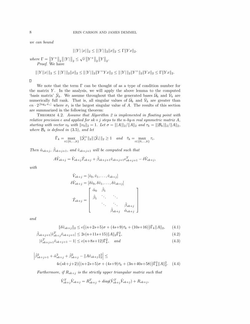
Theorem 4.2. Assume that Algorithm 2 is implemented in floating point withrelative precision ε and applied for sk+j steps to the n-by-n real symmetric matrix A,starting with vector v0 with ‖v0‖2 = 1. Let σ = ‖|A|‖2/‖A‖2 and τk = ‖|Bk|‖2/‖A‖2,where Bk is defined in (3.5), and let

Γk = maxi∈{0,...,k}

‖Y+i ‖2‖|Yi|‖2 ≥ 1 and τk = max

i∈{0,...,k}τi.

Then αsk+j, βsk+j+1, and vsk+j+1 will be computed such that

AVsk+j = Vsk+j Tsk+j + βsk+j+1vsk+j+1eTsk+j+1 − δVsk+j ,

with

Vsk+j = [v0, v1, . . . , vsk+j ]

δVsk+j = [δv0, δv1, . . . , δvsk+j ]

Tsk+j =

α0 β1

β1. . .

. . .

. . .. . . βsk+jβsk+j αsk+j

and

‖δvsk+j‖2 ≤ ε((n+2s+5)σ + (4s+9)τk + (10s+16)

)Γk‖A‖2, (4.1)

βsk+j+1|vTsk+j vsk+j+1| ≤ 2ε(n+11s+15)‖A‖2Γ2k, (4.2)

|vTsk+j+1vsk+j+1 − 1| ≤ ε(n+8s+12)Γ2k, and (4.3)

∣∣∣β2sk+j+1 + α2

sk+j + β2sk+j − ‖Avsk+j‖22

∣∣∣ ≤4ε(sk+j+2)

((n+2s+5)σ + (4s+9)τk + (3n+40s+58)

)Γ2k‖A‖22. (4.4)

Furthermore, if Rsk+j is the strictly upper triangular matrix such that

V Tsk+j Vsk+j = RTsk+j + diag(V Tsk+j Vsk+j) +Rsk+j ,


then

Tsk+jRsk+j −Rsk+j Tsk+j = βsk+j+1VTsk+j vsk+j+1e

Tsk+j+1 +Hsk+j , (4.5)

where Hsk+j is upper triangular with elements η such that

|η1,1| ≤2ε(n+11s+15)‖A‖2Γ2k, and for i ∈ {2, . . . , sk+j+1},

|ηi,i| ≤4ε(n+11s+15)‖A‖2Γ2k,

|ηi−1,i| ≤2ε((n+2s+5)σ+(4s+9)τk + n+18s+28

)Γ2k‖A‖2, and

|η`,i| ≤2ε((n+2s+5)σ+(4s+9)τk+(10s+16)

)Γ2k‖A‖2, for ` ∈ {1, . . . , i−2}.

(4.6)

Remarks. This generalizes Paige [27] as follows. The bounds in Theorem 4.2 giveinsight into how orthogonality is lost in the finite precision s-step Lanczos algorithm.Equation (4.1) bounds the error in the columns of the resulting perturbed Lanczosrecurrence. How far the Lanczos vectors can deviate from unit 2-norm is given in (4.3),and (4.2) bounds how far adjacent vectors are from being orthogonal. The boundin (4.4) describes how close the columns of AVsk+j and Tsk+j are in size. Finally, (4.5)can be thought of as a recurrence for the loss of orthogonality between Lanczos vectors,and shows how errors propagate through the iterations.

One thing to notice about the bounds in Theorem 4.2 is that they depend heavilyon the term Γk, which is a measure of the conditioning of the computed s-step Krylovbases. This indicates that if Γk is controlled in some way to be near constant, i.e.,Γk = O(1), the bounds in Theorem 4.2 will be on the same order as Paige’s analogousbounds for classical Lanczos [27], and thus we can expect orthogonality to be lost ata similar rate. The bounds also suggest that for the s-step variant to have any use,we must have Γk = o(ε−1/2). Otherwise there can be no expectation of orthogonality.Note that ‖|Bk|‖2 should be . ‖|A|‖2 for many practical basis choices.

Comparing to Paige’s result, we can think of sk + j steps of classical Lanczos asthe case where s = 1, with Y0 = In,n (and then vsk+j = v′k,j , Bk = A). In this case

Γk = 1 and τk = σ and our bounds reduce (modulo constants) to those of Paige [27].

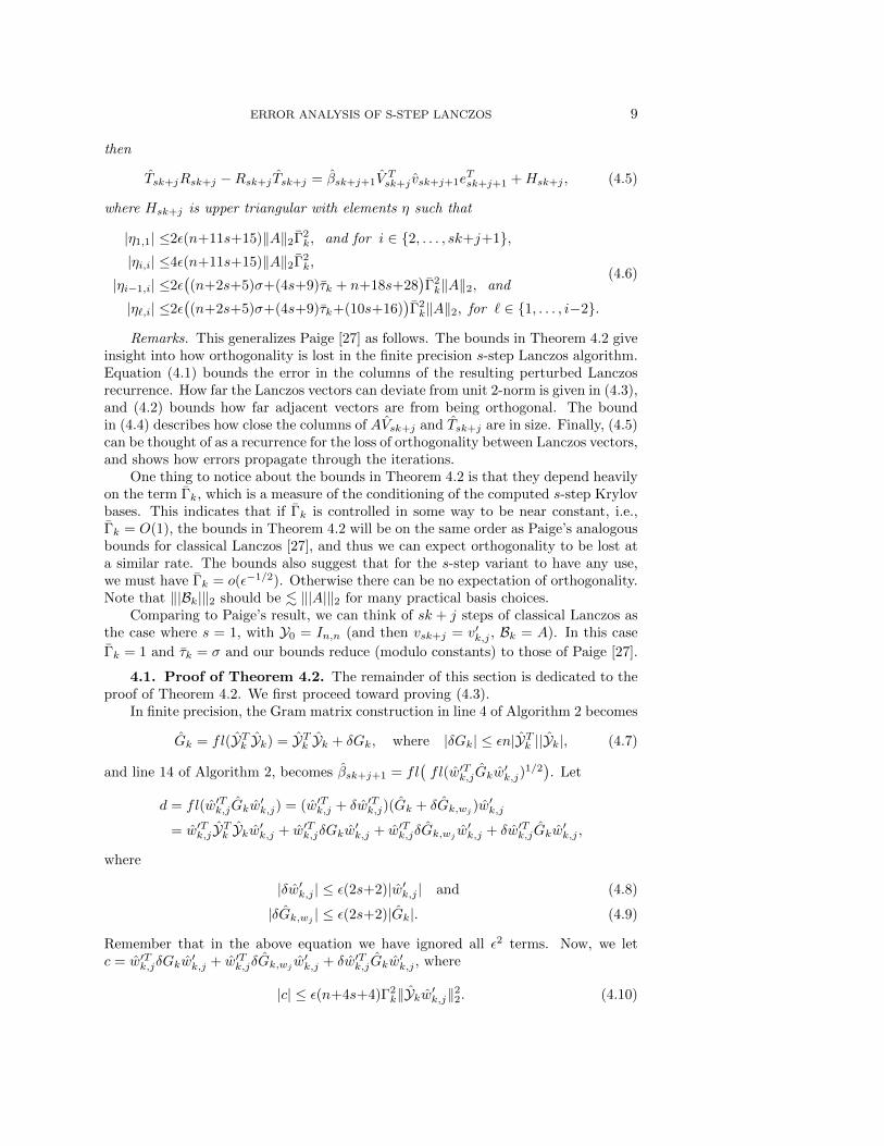
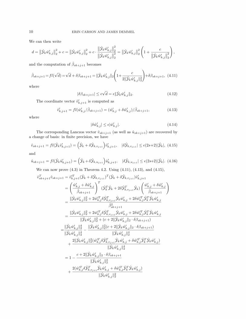
4.1. Proof of Theorem 4.2. The remainder of this section is dedicated to theproof of Theorem 4.2. We first proceed toward proving (4.3).

In finite precision, the Gram matrix construction in line 4 of Algorithm 2 becomes

Gk = fl(YTk Yk) = YTk Yk + δGk, where |δGk| ≤ εn|YTk ||Yk|, (4.7)

and line 14 of Algorithm 2, becomes βsk+j+1 = fl(fl(w′Tk,jGkw

′k,j)

1/2). Let

d = fl(w′Tk,jGkw′k,j) = (w′Tk,j + δw′Tk,j)(Gk + δGk,wj

)w′k,j

= w′Tk,jYTk Ykw′k,j + w′Tk,jδGkw′k,j + w′Tk,jδGk,wj

w′k,j + δw′Tk,jGkw′k,j ,

where

|δw′k,j | ≤ ε(2s+2)|w′k,j | and (4.8)

|δGk,wj| ≤ ε(2s+2)|Gk|. (4.9)

Remember that in the above equation we have ignored all ε2 terms. Now, we letc = w′Tk,jδGkw

′k,j + w′Tk,jδGk,wj

w′k,j + δw′Tk,jGkw′k,j , where

|c| ≤ ε(n+4s+4)Γ2k‖Ykw′k,j‖22. (4.10)


We can then write

d =∥∥Ykw′k,j∥∥22 + c =

∥∥Ykw′k,j∥∥22 + c ·∥∥Ykw′k,j∥∥22∥∥Ykw′k,j∥∥22 =

∥∥Ykw′k,j∥∥22(

1 +c∥∥Ykw′k,j∥∥22

),

and the computation of βsk+j+1 becomes

βsk+j+1 =fl(√d) =√d+ δβsk+j+1 = ‖Ykw′k,j‖2

(1+

c

2‖Ykw′k,j‖22

)+δβsk+j+1, (4.11)

where

|δβsk+j+1| ≤ ε√d = ε‖Ykw′k,j‖2. (4.12)

The coordinate vector v′k,j+1 is computed as

v′k,j+1 = fl(w′k,j/βsk+j+1) = (w′k,j + δw′k,j)/βsk+j+1, (4.13)

where

|δw′k,j | ≤ ε|w′k,j |. (4.14)

The corresponding Lanczos vector vsk+j+1 (as well as usk+j+1) are recovered bya change of basis: in finite precision, we have

vsk+j+1 = fl(Ykv′k,j+1) =(Yk + δYk,vj+1

)v′k,j+1, |δYk,vj+1

| ≤ ε(2s+2)|Yk|, (4.15)

and

usk+j+1 = fl(Yku′k,j+1) =(Yk+δYk,uj+1

)u′k,j+1, |δYk,uj+1

| ≤ ε(2s+2)|Yk|. (4.16)

We can now prove (4.3) in Theorem 4.2. Using (4.11), (4.13), and (4.15),

vTsk+j+1vsk+j+1 = v′Tk,j+1(Yk + δYk,vj+1)T (Yk + δYk,vj+1

)v′k,j+1

=

(w′k,j + δw′k,j

βsk+j+1

)T(YTk Yk + 2δYTk,vj+1

Yk)

(w′k,j + δw′k,j

βsk+j+1

)

=‖Ykw′k,j‖22 + 2w′Tk,jδYTk,vj+1

Ykw′k,j + 2δw′Tk,jYTk Ykw′k,jβ2sk+j+1

=‖Ykw′k,j‖22 + 2w′Tk,jδYTk,vj+1

Ykw′k,j + 2δw′Tk,jYTk Ykw′k,j‖Ykw′k,j‖22 + (c+ 2‖Ykw′k,j‖2 · δβsk+j+1)

=‖Ykw′k,j‖42‖Ykw′k,j‖42

−‖Ykw′k,j‖22(c+ 2‖Ykw′k,j‖2 · δβsk+j+1)

‖Ykw′k,j‖42

+2‖Ykw′k,j‖22(w′Tk,jδYTk,vj+1

Ykw′k,j + δw′Tk,jYTk Ykw′k,j)

‖Ykw′k,j‖42

= 1−c+ 2‖Ykw′k,j‖2 · δβsk+j+1

‖Ykw′k,j‖22

+2(w′Tk,jδYTk,vj+1

Ykw′k,j + δw′Tk,jYTk Ykw′k,j)

‖Ykw′k,j‖22


Now, using bounds in (4.7), (4.8), (4.9), (4.10), (4.15), (4.16), and Lemma 4.1, weobtain

|vTsk+j+1vsk+j+1 − 1| ≤ε(n+4s+4)Γ2k + 2ε+ 2ε(2s+2)Γk + 2εΓk

≤ε(n+4s+4)Γ2k + ε(4s+6)Γk + 2ε

≤ε(n+8s+12)Γ2k.

This thus proves (4.3), and we now proceed toward proving (4.2). Using (4.9), line 12in Algorithm 2 is computed in finite precision as

αsk+j = fl(v′Tk,jGku′k,j) = (v′Tk,j + δv′Tk,j)(Gk + δGk,uj

)u′k,j ,

where |δv′k,j | ≤ ε(2s+2)|v′k,j | and |δGk,uj | ≤ ε(2s + 2)|Gk|. Expanding the aboveequation using (4.7), and (4.15), we obtain

αsk+j =v′Tk,jGku′k,j + v′Tk,jδGk,uj

u′k,j + δv′Tk,jGku′k,j

=v′Tk,j(YTk Yk + δGk)u′k,j + v′Tk,jδGk,uju′k,j + δv′Tk,jGku

′k,j

=v′Tk,jYTk Yku′k,j + v′Tk,jδGku′k,j + v′Tk,jδGk,uj

u′k,j + δv′Tk,jGku′k,j

=(vsk+j − δYk,vj v′k,j)T (usk+j − δYk,uju′k,j) + v′Tk,jδGku

′k,j + v′Tk,jδGk,uj

u′k,j

+ δv′Tk,jGku′k,j

=vTsk+j usk+j + δαsk+j , (4.17)

with δαsk+j = δv′Tk,jGku′k,j + v′Tk,j(δGk + δGk,uj

− YTk δYk,uj− δYTk,vj Yk)u′k,j .

Using bounds in (4.3), (4.7), (4.8), (4.9), (4.15), and (4.16), as well as Lemma 4.1,we can write (again, ignoring ε2 terms),

|δαsk+j | ≤ε(n+8s+8)|v′Tk,j ||YTk ||Yk||u′k,j |

≤ε(n+8s+8) ‖|Yk||v′k,j |‖2 ‖|Yk||u′k,j |‖2≤ε(n+8s+8)(Γk‖vsk+j‖2)(Γk‖usk+j‖2)

≤ε(n+8s+8)(Γk(1 + (ε/2)(n+8s+12)Γ2

k))(Γk‖usk+j‖2)

≤ε(n+8s+8)Γk(Γk‖usk+j‖2)

≤ε(n+8s+8)Γ2k

∥∥usk+j∥∥2. (4.18)

Taking the norm of (4.17), and using the bounds in (4.18) and (4.3), we obtain thebound

|αsk+j | ≤‖vTsk+j‖2‖usk+j‖2 + |δαsk+j |≤(1 + (ε/2)(n+8s+12)Γ2

k

)‖usk+j‖2 + ε(n+8s+8)Γ2

k‖usk+j‖2

≤(

1 + ε((3/2)n+12s+14

)Γ2k

)‖usk+j‖2. (4.19)

In finite precision, line 13 of Algorithm 2 is computed as

w′k,j = u′k,j − αsk+j v′k,j − δw′k,j , where |δw′k,j | ≤ ε(|u′k,j |+ 2|αsk+j v′k,j |). (4.20)

Multiplying both sides of (4.20) by Yk gives

Ykw′k,j = Yku′k,j − αsk+jYkv′k,j − Ykδw′k,j ,


and multiplying each side by its own transpose, we get

w′Tk,jYTk Ykw′k,j = (Yku′k,j−αsk+jYkv′k,j−Ykδw′k,j)T (Yku′k,j−αsk+jYkv′k,j−Ykδw′k,j)

= u′Tk,jYTk Yku′k,j − 2αsk+j u′Tk,jYTk Ykv′k,j + α2

sk+j v′Tk,jYTk Ykv′k,j

− δw′Tk,jYTk (Yku′k,j−αsk+jYkv′k,j)−(Yku′k,j−αsk+jYkv′k,j)T Ykδw′k,j .

Using (4.15) and (4.16), we can write

w′Tk,jYTk Ykw′k,j = (usk+j − δYk,uj u′k,j)

T (usk+j − δYk,uj u′k,j)

− 2αsk+j(usk+j − δYk,uj u′k,j)

T (vsk+j − δYk,vj v′k,j)

+ α2sk+j(vsk+j − δYk,vj v′k,j)T (vsk+j − δYk,vj v′k,j)

− 2δw′Tk,jYTk (Yku′k,j − αsk+jYkv′k,j)

= uTsk+j usk+j − 2uTsk+jδYk,uju′k,j − 2αsk+j u

Tsk+j vsk+j

+ 2αsk+j uTsk+jδYk,vj v′k,j + 2αsk+j u

′Tk,jδYTk,uj

vsk+j

+ α2sk+j v

Tsk+j vsk+j − 2α2

sk+j vTsk+jδYk,vj v′k,j

− 2δw′Tk,jYTk (Yku′k,j − αsk+jYkv′k,j)= uTsk+j usk+j − 2αsk+j u

Tsk+j vsk+j + α2

sk+j vTsk+j vsk+j

− 2(δYk,uju′k,j − αsk+jδYk,vj v′k,j)T (usk+j − αsk+j vsk+j)

− 2δw′Tk,jYTk (Yku′k,j − αsk+jYkv′k,j).

This can be written

‖Ykw′k,j‖22 = ‖usk+j‖22 − 2αsk+j uTsk+j vsk+j + α2

sk+j‖vsk+j‖22− 2(δYk,uj

u′k,j − αsk+jδYk,vj v′k,j + Ykδw′k,j)T (usk+j − αsk+j vsk+j),

where we have used Yku′k,j − αsk+jYkv′k,j = usk+j − αsk+j vsk+j + O(ε). Now, us-ing (4.17),

‖Ykw′k,j‖22 = ‖usk+j‖22 − 2αsk+j(αsk+j − δαsk+j) + α2sk+j‖vsk+j‖22

− 2(δYk,uj u′k,j − αsk+jδYk,vj v′k,j + Ykδw′k,j)T (usk+j − αsk+j vsk+j)

= ‖usk+j‖22 + α2sk+j(‖vsk+j‖22 − 2) + 2αsk+jδαsk+j

− 2(δYk,uju′k,j − αsk+jδYk,vj v′k,j + Ykδw′k,j)T (usk+j − αsk+j vsk+j).

Now, we rearrange the above equation to obtain

‖Ykw′k,j‖22 + α2sk+j − ‖usk+j‖22 = α2

sk+j(‖vsk+j‖22 − 1) + 2αsk+jδαsk+j

− 2(δYk,uju′k,j − αsk+jδYk,vj v′k,j + Ykδw′k,j)T (usk+j − αsk+j vsk+j).

Using Lemma 4.1 and bounds in (4.3), (4.15), (4.16), (4.18), (4.19), and (4.20),


we can then write

‖Ykw′k,j‖22+α2sk+j−‖usk+j‖22 ≤

(1+ε

((3/2)n+12s+14

)Γ2k

)2· ε(n+8s+12)Γ2

k‖usk+j‖22

+ 2(1+ε

((3/2)n+12s+14

)Γ2k

)· ε(n+8s+8)Γ2

k‖usk+j‖22+ 2ε

((2s+2) + (2s+2) + 3

)Γk‖usk+j‖2 · 2‖usk+j‖2

≤ ε(n+8s+12)Γ2k‖usk+j‖22 + 2ε(n+8s+8)Γ2

k‖usk+j‖22+ ε(16s+28)Γk‖usk+j‖22,

where, again, we have ignored ε2 terms. Using Γk ≤ Γ2k, this gives the bound

‖Ykw′k,j‖22 + α2sk+j − ‖usk+j‖22 ≤ ε(3n+40s+56)Γ2

k‖usk+j‖22. (4.21)

Given the above, we can also write the bound

‖Ykw′k,j‖22 ≤ ‖Ykw′k,j‖22 + α2sk+j ≤

(1 + ε(3n+40s+56)Γ2

k

)‖usk+j‖22, (4.22)

and using (4.10), (4.11), and (4.12),

|βsk+j+1| ≤ ‖Ykw′k,j‖2

(1 + ε+

c

2‖Ykw′k,j‖22

)

≤(1 + (1/2)ε(3n+40s+56)Γ2

k

)‖usk+j‖2

(1 + ε+

c

2‖Ykw′k,j‖22

)≤(1 + ε+ (1/2)ε(n+4s+4)Γ2

k + (1/2)ε(3n+40s+56)Γ2k

)‖usk+j‖2.

Combining terms and using 1 ≤ Γ2k, the above can be written

|βsk+j+1| ≤(1 + ε(2n+22s+31)Γ2

k

)∥∥usk+j∥∥2. (4.23)

Now, rearranging (4.13), we can write

βsk+j+1v′k,j+1 = w′k,j + δw′k,j ,

and premultiplying by Yk, we obtain

βsk+j+1Ykv′k,j+1 = Ykw′k,j + Ykδw′k,j .

Using (4.15), this can be written

βsk+j+1(vsk+j+1 − δYk,vj+1v′k,j+1) = Ykw′k,j + Ykδw′k,j .

Rearranging and using (4.13),

βsk+j+1vsk+j+1 = Ykw′k,j + Ykδw′k,j + βsk+j+1δYk,vj+1v′k,j+1

= Ykw′k,j + Ykδw′k,j + δYk,vj+1(w′k,j + δw′k,j)

= Ykw′k,j + Ykδw′k,j + δYk,vj+1w′k,j

≡ Ykw′k,j + δwsk+j , (4.24)


where δwsk+j = Ykδw′k,j + δYk,vj+1w′k,j . Using Lemma 4.1 and bounds in (4.14),

(4.15), and (4.22),

‖δwsk+j‖2 ≤ ε‖|Yk||w′k,j |‖2 + ε(2s+2)‖|Yk||w′k,j |‖2≤ ε(2s+3)Γk‖Ykw′k,j‖2≤ ε(2s+3)Γk‖usk+j‖2. (4.25)

We premultiply (4.24) by vTsk+j and use (4.15), (4.16), (4.17), and (4.20) to obtain

βsk+j+1vTsk+j vsk+j+1 = vTsk+j(Ykw′k,j + δwsk+j)

= vTsk+j(Yku′k,j − αsk+jYkv′k,j − Ykδw′k,j) + vTsk+jδwsk+j

= vTsk+j(Yku′k,j − αsk+jYkv′k,j

)− vTsk+j

(Ykδw′k,j − δwsk+j

)= vTsk+j

((usk+j − δYk,uj u

′k,j)− αsk+j(vsk+j − δYk,vj v′k,j)

)− vTsk+j(Ykδw′k,j − δwsk+j)

= vTsk+j usk+j − αsk+j vTsk+j vsk+j− vTsk+j(δYk,uj

u′k,j − αsk+jδYk,vj v′k,j + Ykδw′k,j − δwsk+j)= (αsk+j − δαsk+j)− αsk+j‖vsk+j‖22− vTsk+j(δYk,uj u

′k,j − αsk+jδYk,vj v′k,j + Ykδw′k,j − δwsk+j)

= −δαsk+j − αsk+j(‖vsk+j‖22 − 1)

− vTsk+j(δYk,uju′k,j − αsk+jδYk,vj v′k,j + Ykδw′k,j − δwsk+j),

and using Lemma 4.1 and bounds in (4.3), (4.13), (4.15), (4.16), (4.18), (4.19), (4.20),and (4.25), we can write the bound∣∣∣βsk+j+1 · vTsk+j vsk+j+1

∣∣∣ ≤ |δαsk+j |+ |αsk+j ||vTsk+j vsk+j − 1|

+ ‖vsk+j‖2(‖|δYk,uj

||u′k,j |‖2 + |αsk+j |‖|δYk,vj ||v′k,j |‖2)

+ ‖vsk+j‖2(‖|Yk||δw′k,j |‖2 + ‖δwsk+j‖2

)≤ 2ε(n+11s+15)Γ2

k‖usk+j‖2. (4.26)

This is a start toward proving (4.2). We will return to the above bound once welater prove a bound on ‖usk+j‖2. Our next step is to analyze the error in each columnof the finite precision s-step Lanczos recurrence. First, we note that we can write theerror in computing the s-step bases (line 3 in Algorithm 2) by

AYk = YkBk + δEk (4.27)

where Yk =[Vk[Is, 0s,1]T , 0n,1, Uk[Is, 0s,1]T , 0n,1

]. It can be shown (see, e.g., [3]) that

if the basis is computed in the usual way by repeated SpMVs,

|δEk| ≤ ε((3+n)|A||Yk|+ 4|Yk||Bk|

). (4.28)

In finite precision, line 17 in Algorithm 2 is computed as

u′k,j =Bkv′k,j−βsk+j v′k,j−1+δu′k,j , |δu′k,j | ≤ ε((2s+3)|Bk||v′k,j |+2|βsk+j v′k,j−1|

), (4.29)


and then, with Lemma 4.1, (4.15), (4.16), (4.27), and (4.29), we can write

usk+j = (Yk + δYk,uj)u′k,j

= (Yk + δYk,uj )(Bkv′k,j − βsk+j v′k,j−1 + δu′k,j)

= YkBkv′k,j − βsk+jYkv′k,j−1 + Ykδu′k,j + δYk,ujBkv′k,j − βsk+jδYk,uj

v′k,j−1

= (AYk − δEk)v′k,j − βsk+j(vsk+j−1 − δYk,vj−1 v′k,j−1) + Ykδu′k,j

+ δYk,ujBkv′k,j − βsk+jδYk,uj

v′k,j−1

= AYkv′k,j − δEkv′k,j − βsk+j vsk+j−1 + βsk+jδYk,vj−1

v′k,j−1 + Ykδu′k,j+ δYk,ujBkv′k,j − βsk+jδYk,uj v

′k,j−1

= A(vsk+j − δYk,vj v′k,j)− δEkv′k,j − βsk+j vsk+j−1 + βsk+jδYk,vj−1v′k,j−1

+ Ykδu′k,j + δYk,ujBkv′k,j − βsk+jδYk,uj v′k,j−1

= Avsk+j −AδYk,vj v′k,j − δEkv′k,j − βsk+j vsk+j−1 + βsk+jδYk,vj−1v′k,j−1

+ Ykδu′k,j + δYk,ujBkv′k,j − βsk+jδYk,uj

v′k,j−1

≡ Avsk+j − βsk+j vsk+j−1 + δusk+j , (4.30)

where

δusk+j = Ykδu′k,j − (AδYk,vj − δYk,ujBk + δEk)v′k,j + βsk+j(δYk,vj−1 − δYk,uj)v′k,j−1.

Using the bounds in (4.15), (4.16), (4.23), (4.28), and (4.29) we can write

|δusk+j | ≤ ε((2s+3)|Yk||Bk||v′k,j |+ 2|βsk+j ||Yk||v′k,j−1|

)+ ε(2s+2)|A||Yk||v′k,j |+ ε(2s+2)|Yk||Bk||v′k,j |

+ ε((3+n)|A||Yk||v′k,j |+ 4|Yk||Bk||v′k,j |

)+ 2ε(2s+2)|βsk+j ||Yk||v′k,j−1|

≤ ε(n+2s+5)|A||Yk||v′k,j |+ ε(4s+9)|Yk||Bk||v′k,j |

+ ε(4s+6)(1 + ε(2n+22s+31)Γ2

k

)‖usk+j−1‖2 · |Yk||v′k,j−1|.

and from this we obtain

‖δusk+j‖2 ≤ ε(n+2s+5) ‖|A|‖2 ‖|Yk|‖2 ‖v′k,j‖2 + ε(4s+9) ‖|Yk|‖2 ‖|Bk|‖2 ‖v′k,j‖2+ ε(4s+6) ‖|Yk|‖2 ‖v′k,j−1‖2 ‖usk+j−1‖2≤ ε(n+2s+5) ‖|A|‖2 Γk + ε(4s+9) ‖|Bk|‖2 Γk + ε(4s+6) ‖usk+j−1‖2 Γk.

We will now introduce and make use of the quantities σ ≡ ‖|A|‖2/‖A‖2 and τk ≡‖|Bk|‖2/‖A‖2. Note that the quantity ‖|Bk|‖2 is controlled by the user, and for manypopular basis choices, such as monomial, Newton, or Chebyshev bases, it should bethe case that ‖|Bk|‖2 . ‖|A|‖2. Using these quantities, the bound above can bewritten∥∥δusk+j∥∥2 ≤ ε(((n+2s+5)σ + (4s+9)τk

)‖A‖2 + (4s+6)‖usk+j−1‖2

)Γk. (4.31)


Manipulating (4.24), and using (4.15), (4.16), and (4.20), we have

βsk+j+1vsk+j+1 = Ykw′k,j + δwsk+j

= Yku′k,j − αsk+jYkv′k,j − Ykδw′k,j + δwsk+j

= (usk+j−δYk,uju′k,j)−αsk+j(vsk+j−δYk,vj v′k,j)−Ykδw′k,j+δwsk+j

= usk+j−αsk+j vsk+j−δYk,uj u′k,j+αsk+jδYk,vj v′k,j−Ykδw′k,j

+ δwsk+j ,

and substituting in the expression for usk+j in (4.30) on the right, we obtain

βsk+j+1vsk+j+1 ≡ Avsk+j − αsk+j vsk+j − βsk+j vsk+j−1 + δvsk+j , (4.32)

where

δvsk+j = δusk+j − δYk,uj u′k,j + αsk+jδYk,vj v′k,j − Ykδw′k,j + δwsk+j .

From this we can write the componentwise bound

|δvsk+j | ≤ |δusk+j |+ |δYk,uj | |u′k,j |+ |αsk+j | |δYk,vj | |v′k,j |+ |Yk| |δw′k,j |+ |δwsk+j |,

and using Lemma 4.1, (4.14), (4.15), (4.16), (4.19), (4.20), and (4.25) we obtain

‖δvsk+j‖2 ≤ ‖δusk+j‖2 + ε(2s+2)‖|Yk||u′k,j |‖2+(1 + ε((3/2)n+12s+14)Γ2

k

)‖usk+j‖2 · ε(2s+2)‖|Yk||v′k,j |‖2

+ ε‖|Yk||u′k,j |‖2 + 2ε(1 + ε((3/2)n+12s+14)Γ2

k

)‖usk+j‖2‖|Yk||v′k,j |‖2

+ ε(2s+3)Γk‖usk+j‖2≤ ‖δusk+j‖2 + ε(2s+2)Γk‖usk+j‖2 + ε(2s+2)Γk‖usk+j‖2

+ εΓk‖usk+j‖2 + 2εΓk‖usk+j‖2 + ε(2s+3)Γk‖usk+j‖2≤ ‖δusk+j‖2 + ε(6s+10)Γk‖usk+j‖2.

Using (4.31), this gives the bound

‖δvsk+j‖2 ≤

ε((

(n+2s+5)σ+(4s+9)τk)‖A‖2+(6s+10)‖usk+j‖2+(4s+6)‖usk+j−1‖2

)Γk. (4.33)

We now have everything we need to write the finite-precision s-step Lanczosrecurrence in its familiar matrix form. Let

Tsk+j =

α0 β1

β1. . .

. . .

. . .. . . βsk+j

βsk+j αsk+j

,

and let Vsk+j = [v0, v1, . . . , vsk+j ] and δVsk+j = [δv0, δv1, . . . , δvsk+j ]. Note that

Tsk+j has dimension (sk+j+1)-by-(sk+j+1), and Vsk+j and δVsk+j have dimensionn-by-(sk + j + 1). Then (4.32) in matrix form gives

AVsk+j = Vsk+j Tsk+j + βsk+j+1vsk+j+1eTsk+j+1 − δVsk+j . (4.34)


Thus (4.33) gives a bound on the error in the columns of the finite precision s-stepLanczos recurrence. Again, we will return to (4.33) to prove (4.1) once we bound‖usk+j‖2.

Now, we examine the possible loss of orthogonality in the vectors v0, . . . , vsk+j+1.We define the strictly upper triangular matrix Rsk+j of dimension (sk + j + 1)-by-(sk + j + 1) with elements ρi,j , for i, j ∈ {1, . . . , sk + j + 1}, such that

V Tsk+j Vsk+j = RTsk+j + diag(V Tsk+j Vsk+j) +Rsk+j .

For notational purposes, we also define ρsk+j+1,sk+j+2 ≡ vTsk+j vsk+j+1. (Note thatρsk+j+1,sk+j+2 is not an element in Rsk+j , but would be an element in Rsk+j+1).

Multiplying (4.34) on the left by V Tsk+j , we get

V Tsk+jAVsk+j = V Tsk+j Vsk+j Tsk+j + βsk+j+1VTsk+j vsk+j+1e

Tsk+j+1 − V Tsk+jδVsk+j .

Since the above is symmetric, we can equate the right hand side by its own transposeto obtain

Tsk+j(RTsk+j +Rsk+j)− (RTsk+j +Rsk+j)Tsk+j =

βsk+j+1(V Tsk+j vsk+j+1eTsk+j+1 − esk+j+1v

Tsk+j+1Vsk+j)

+ V Tsk+jδVsk+j−δV Tsk+j Vsk+j +diag(V Tsk+j Vsk+j) · Tsk+j− Tsk+j ·diag(V Tsk+j Vsk+j).

Now, let Msk+j ≡ Tsk+jRsk+j − Rsk+j Tsk+j , which is upper triangular and hasdimension (sk+ j + 1)-by-(sk+ j + 1). Then the left-hand side above can be writtenas Msk+j −MT

sk+j , and we can equate the strictly upper triangular part of Msk+j

with the strictly upper triangular part of the right-hand side above. The diagonalelements can be obtained from the definition Msk+j ≡ Tsk+jRsk+j−Rsk+j Tsk+j , i.e.,

m1,1 =− β1ρ1,2, msk+j+1,sk+j+1 = βsk+jρsk+j,sk+j+1, and

mi,i =βi−1ρi−1,i − βiρi,i+1, for i ∈ {2, . . . , sk + j}.

Therefore, we can write

Msk+j = Tsk+jRsk+j −Rsk+j Tsk+j = βsk+j+1VTsk+j vsk+j+1e

Tsk+j+1 +Hsk+j ,

where Hsk+j has elements satisfying

η1,1 =− β1ρ1,2,

ηi,i =βi−1ρi−1,i − βiρi,i+1, for i ∈ {2, . . . , sk+j+1},

ηi−1,i =vTi−2δvi−1 − δvTi−2vi−1 + βi−1(vTi−2vi−2 − vTi−1vi−1), and

η`,i =vT`−1δvi−1 − δvT`−1vi−1, for ` ∈ {1, . . . , i− 2}.

(4.35)

To simplify notation, we introduce the quantities

usk+j = maxi∈{0,...,sk+j}

‖ui‖2, Γk = maxi∈{0,...,k}

Γi, and τk = maxi∈{0,...,k}

τi.


Using this notation and (4.3), (4.23), (4.26), and (4.33), the quantities in (4.35) canbe bounded by

|η1,1| ≤ 2ε(n+11s+15)Γ2k usk+j , and, for i ∈ {2, . . . , sk+j+1},

|ηi,i| ≤ 4ε(n+11s+15)Γ2k usk+j ,

|ηi−1,i| ≤ 2ε((

(n+2s+5)σ + (4s+9)τk)‖A‖2 + (n+18s+28)usk+j

)Γ2k, and

|η`,i| ≤ 2ε((

(n+2s+5)σ+(4s+9)τk)‖A‖2+(10s+16)usk+j

)Γ2k,

(4.36)

for ` ∈ {1, . . . , i−2}.The above is a start toward proving (4.6). We return to this bound later, and

now shift our focus towards proving a bound on ‖usk+j‖2. To proceed, we must firstfind a bound for |vTsk+j vsk+j−2|. From the definition of Msk+j , we know the (1, 2)element of Msk+j is

α0ρ1,2 − α1ρ1,2 − β2ρ1,3 = η1,2,

and for i > 2, the (i−1, i) element is

βi−2ρi−2,i + (αi−2 − αi−1)ρi−1,i − βiρi−1,i+1 = ηi−1,i.

Then, defining

ξi ≡ (αi−2 − αi−1)βi−1ρi−1,i − βi−1ηi−1,i

for i ∈ {2, . . . , sk+j}, we have

βi−1βiρi−1,i+1 = βi−2βi−1ρi−2,i + ξi = ξi + ξi−1 + . . .+ ξ2.

This, along with (4.19), (4.23), (4.26), and (4.36) gives

βsk+j−1βsk+j |ρsk+j−1,sk+j+1| = βsk+j−1βsk+j |vTsk+j−2vsk+j |

≤sk+j∑i=2

|ξi| ≤sk+j∑i=2

(|αi−2|+ |αi−1|)|βi−1ρi−1,i|+ |βi−1||ηi−1,i|

≤2ε

sk+j∑i=2

(((n+2s+5)σ+(4s+9)τk

)‖A‖2 +(3n+40s+58)usk+j

)Γ2kusk+j

≤2ε(sk+j−1)((

(n+2s+5)σ+(4s+9)τk)‖A‖2 +(3n+40s+58)usk+j

)Γ2kusk+j .

(4.37)

Rearranging (4.30) gives

usk+j − δusk+j = Avsk+j − βsk+j vsk+j−1,

and multiplying each side by its own transpose (ignoring ε2 terms), we obtain

uTsk+j usk+j − 2uTsk+jδusk+j = ‖Avsk+j‖22+β2sk+j‖vsk+j−1‖22−2βsk+j v

Tsk+jAvsk+j−1.

(4.38)Rearranging (4.32) gives

Avsk+j−1 = βsk+j vsk+j + αsk+j−1vsk+j−1 + βsk+j−1vsk+j−2 − δvsk+j−1,


and premultiplying this expression by βsk+j vTsk+j , we get

βsk+j vTsk+jAvsk+j−1

=βsk+j vTsk+j

(βsk+j vsk+j + αsk+j−1vsk+j−1 + βsk+j−1vsk+j−2 − δvsk+j−1

)=β2

sk+j‖vsk+j‖22 + αsk+j−1(βsk+j vTsk+j vsk+j−1) + βsk+j βsk+j−1v

Tsk+j vsk+j−2

− βsk+j vTsk+jδvsk+j−1≡β2

sk+j + δβsk+j , (4.39)

where, using bounds in (4.3), (4.19), (4.23), (4.26), (4.33), and (4.37),

|δβsk+j | ≤ ε((

(n+2s+5)σ + (4s+9)τk)‖A‖2 + (3n+40s+58)usk+j

)Γ2kusk+j (4.40)

+2ε(sk+j−1)((

(n+2s+5)σ+(4s+9)τk)‖A‖2+(3n+40s+58)usk+j

)Γ2kusk+j .

Adding 2uTsk+jδusk+j to both sides of (4.38) and using (4.39), we obtain

‖usk+j‖22 = ‖Avsk+j‖22 + β2sk+j

(‖vsk+j−1‖22 − 2

)− 2δβsk+j + 2uTsk+jδusk+j

≡ ‖Avsk+j‖22 + β2sk+j

(‖vsk+j−1‖22 − 2

)+ δβsk+j , (4.41)

where δβsk+j = −2δβsk+j+2uTsk+jδusk+j , and, using the bounds in (4.31) and (4.40),

|δβsk+j |≤ 2|δβsk+j |+ 2‖uTsk+j‖2‖δusk+j‖2

≤ 4ε(sk+j)((

(n+2s+5)σ+(4s+9)τk)‖A‖2 + (3n+40s+58)usk+j

)Γ2kusk+j

+ 2ε((

(n+2s+5)σ+(4s+9)τk)‖A‖2 + (4s+6)usk+j

)Γ2kusk+j

≤ 4ε(sk+j+1)((

(n+2s+5)σ+(4s+9)τk)‖A‖2+(3n+40s+58)usk+j

)Γ2kusk+j .

(4.42)

Now, using (4.41), and since β2sk+j ≥ 0, we can write

‖usk+j‖22≤‖usk+j‖22+β2sk+j ≤‖A‖22‖vsk+j‖22+β2

sk+j

(‖vsk+j−1‖22−1

)+|δβsk+j |. (4.43)

Let µ ≡ max{usk+j , ‖A‖2

}. Then (4.43) along with bounds in (4.3), (4.23), and (4.42)

gives

‖usk+j‖22≤‖A‖22+4ε(sk+j+2)((n+2s+5)σ+(4s+9)τk+(3n+40s+58)

)Γ2kµ

2. (4.44)

We consider the two possible cases for µ. First, if µ = ‖A‖2, then

‖usk+j‖22 ≤ ‖A‖22 + 4ε(sk+j+2)((n+2s+5)σ + (4s+9)τk + (3n+40s+58)

)Γ2k‖A‖22

≤ ‖A‖22(

1 + 4ε(sk+j+2)((n+2s+5)σ + (4s+9)τk + (3n+40s+58)

)Γ2k

).

Otherwise, we have the case µ = usk+j . Since the bound in (4.44) holds for all‖usk+j‖22, it also holds for u2sk+j = µ2, and thus, ignoring terms of order ε2,

µ2 ≤ ‖A‖22 + 4ε(sk+j+2)((n+2s+5)σ + (4s+9)τk + (3n+40s+58)

)Γ2kµ

2

≤ ‖A‖22 + 4ε(sk+j+2)((n+2s+5)σ + (4s+9)τk + (3n+40s+58)

)Γ2k‖A‖22

≤ ‖A‖22(

1 + 4ε(sk+j+2)((n+2s+5)σ + (4s+9)τk + (3n+40s+58)

)Γ2k

),


and, plugging this in to (4.44), we get

‖usk+j‖22≤‖A‖22(1+4ε(sk+j+2)

((n+2s+5)σ+(4s+9)τk+(3n+40s+58)

)Γ2k

). (4.45)

In either case we obtain the same bound on ‖usk+j‖22, so (4.45) holds.Taking the square root of (4.45), we have

‖usk+j‖2 ≤ ‖A‖2(

1+2ε(sk+j+2)((n+2s+5)σ+(4s+9)τk+(3n+40s+58)

)Γ2k

), (4.46)

and substituting (4.46) into (4.26), (4.33), and (4.36) proves the bounds (4.2), (4.1),and (4.6) in Theorem 4.2, respectively, assuming that

2ε(sk+j+2)((n+2s+5)σ + (4s+9)τk + (3n+40s+58)

)Γ2k � 1.

The only remaining inequality to prove is (4.4). To do this, we first multiply bothsides of (4.24) by their own transposes to obtain

β2sk+j+1‖vsk+j+1‖22 = ‖Ykw′k,j‖22 + 2δwTsk+jYkw′k,j .

Adding α2sk+j − ‖usk+j‖22 to both sides,

β2sk+j+1‖vsk+j+1‖22 + α2

sk+j − ‖usk+j‖22 = ‖Ykw′k,j‖22 + α2sk+j − ‖usk+j‖22

+ 2δwTsk+jYkw′k,j .

Substituting in (4.41) on the left hand side,

β2sk+j+1‖vsk+j+1‖22 + α2

sk+j − ‖Avsk+j‖22 − β2sk+j(‖vsk+j−1‖22 − 2)− δβsk+j =

‖Ykw′k,j‖22 + α2sk+j − ‖usk+j‖22 + 2δwTsk+jYkw′k,j ,

and then subtracting β2sk+j+1 from both sides gives

β2sk+j+1(‖vsk+j+1‖22 − 1) + α2

sk+j − ‖Avsk+j‖22 − β2sk+j(‖vsk+j−1‖22 − 2)− δβsk+j =

‖Ykw′k,j‖22 + α2sk+j − ‖usk+j‖22 + 2δwTsk+jYkw′k,j − β2

sk+j+1.

This can be rearranged to give

β2sk+j+1 + α2

sk+j + β2sk+j − ‖Avsk+j‖22 = ‖Ykw′k,j‖22 + α2

sk+j − ‖usk+j‖22+ 2δwTsk+jYkw′k,j + β2

sk+j(‖vsk+j−1‖22 − 1)

− β2sk+j+1(‖vsk+j+1‖22 − 1) + δβsk+j ,

and finally, using (4.3), (4.21), (4.23), (4.25), and (4.42) gives the bound∣∣∣β2sk+j+1 + α2

sk+j + β2sk+j − ‖Avsk+j‖22

∣∣∣ ≤4ε(sk+j+2)

((n+2s+5)σ + (4s+9)τk + (3n+40s+58)

)Γ2k‖A‖22.

This proves (4.4) and thus completes the proof of Theorem 4.2.


0 50 100 150 20010

−17

10−10

100

1010

1020

Iteration

Normality, classical Lanczos

0 50 100 150 20010

−17

10−10

100

1010

1020

Iteration

Orthogonality, classical Lanczos

0 50 100 150 20010

−17

10−10

100

1010

1020

Iteration

ColBound, classical Lanczos

0 50 100 150 20010

−17

10−10

100

1010

1020

Iteration

Diffbound, classical Lanczos

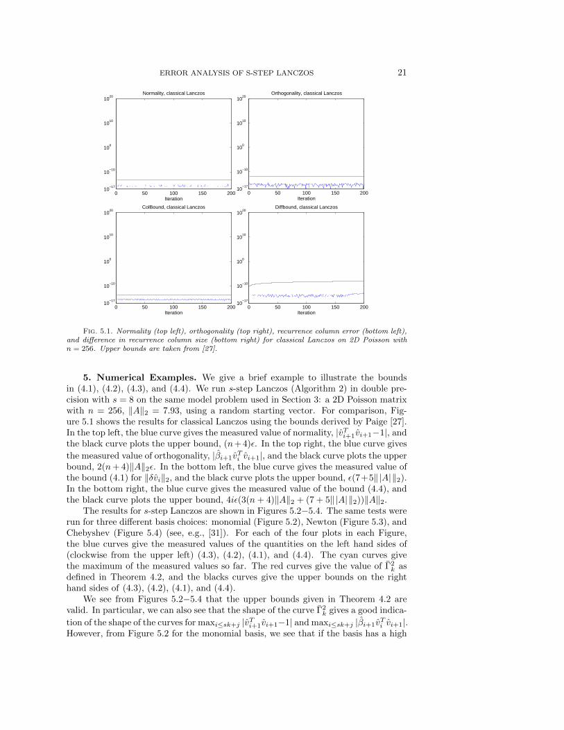
Fig. 5.1. Normality (top left), orthogonality (top right), recurrence column error (bottom left),and difference in recurrence column size (bottom right) for classical Lanczos on 2D Poisson withn = 256. Upper bounds are taken from [27].

5. Numerical Examples. We give a brief example to illustrate the boundsin (4.1), (4.2), (4.3), and (4.4). We run s-step Lanczos (Algorithm 2) in double pre-cision with s = 8 on the same model problem used in Section 3: a 2D Poisson matrixwith n = 256, ‖A‖2 = 7.93, using a random starting vector. For comparison, Fig-ure 5.1 shows the results for classical Lanczos using the bounds derived by Paige [27].In the top left, the blue curve gives the measured value of normality, |vTi+1vi+1−1|, andthe black curve plots the upper bound, (n+ 4)ε. In the top right, the blue curve gives

the measured value of orthogonality, |βi+1vTi vi+1|, and the black curve plots the upper

bound, 2(n+ 4)‖A‖2ε. In the bottom left, the blue curve gives the measured value ofthe bound (4.1) for ‖δvi‖2, and the black curve plots the upper bound, ε(7+5‖|A|‖2).In the bottom right, the blue curve gives the measured value of the bound (4.4), andthe black curve plots the upper bound, 4iε(3(n+ 4)‖A‖2 + (7 + 5‖|A|‖2))‖A‖2.

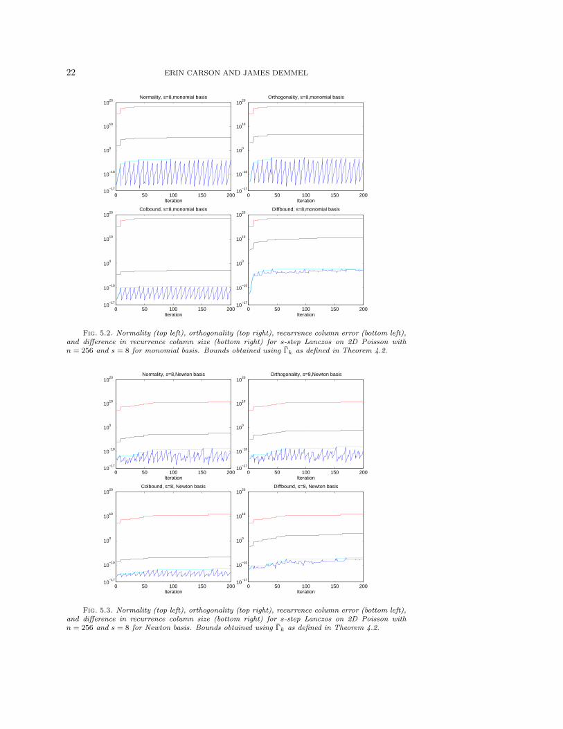
The results for s-step Lanczos are shown in Figures 5.2−5.4. The same tests wererun for three different basis choices: monomial (Figure 5.2), Newton (Figure 5.3), andChebyshev (Figure 5.4) (see, e.g., [31]). For each of the four plots in each Figure,the blue curves give the measured values of the quantities on the left hand sides of(clockwise from the upper left) (4.3), (4.2), (4.1), and (4.4). The cyan curves givethe maximum of the measured values so far. The red curves give the value of Γ2

k asdefined in Theorem 4.2, and the blacks curves give the upper bounds on the righthand sides of (4.3), (4.2), (4.1), and (4.4).

We see from Figures 5.2−5.4 that the upper bounds given in Theorem 4.2 arevalid. In particular, we can also see that the shape of the curve Γ2

k gives a good indica-

tion of the shape of the curves for maxi≤sk+j |vTi+1vi+1−1| and maxi≤sk+j |βi+1vTi vi+1|.

However, from Figure 5.2 for the monomial basis, we see that if the basis has a high


0 50 100 150 20010

−17

10−10

100

1010

1020

Normality, s=8,monomial basis

Iteration0 50 100 150 200

10−17

10−10

100

1010

1020

Orthogonality, s=8,monomial basis

Iteration

0 50 100 150 20010

−17

10−10

100

1010

1020

Colbound, s=8,monomial basis

Iteration0 50 100 150 200

10−17

10−10

100

1010

1020

Diffbound, s=8,monomial basis

Iteration

Fig. 5.2. Normality (top left), orthogonality (top right), recurrence column error (bottom left),and difference in recurrence column size (bottom right) for s-step Lanczos on 2D Poisson withn = 256 and s = 8 for monomial basis. Bounds obtained using Γk as defined in Theorem 4.2.

0 50 100 150 20010

−17

10−10

100

1010

1020

Normality, s=8,Newton basis

Iteration0 50 100 150 200

10−17

10−10

100

1010

1020

Orthogonality, s=8,Newton basis

Iteration

0 50 100 150 20010

−17

10−10

100

1010

1020

Colbound, s=8, Newton basis

Iteration0 50 100 150 200

10−17

10−10

100

1010

1020

Diffbound, s=8, Newton basis

Iteration

Fig. 5.3. Normality (top left), orthogonality (top right), recurrence column error (bottom left),and difference in recurrence column size (bottom right) for s-step Lanczos on 2D Poisson withn = 256 and s = 8 for Newton basis. Bounds obtained using Γk as defined in Theorem 4.2.


0 50 100 150 20010

−17

10−10

100

1010

1020

Normality, s=8,Chebyshev basis

Iteration0 50 100 150 200

10−17

10−10

100

1010

1020

Orthogonality, s=8,Chebyshev basis

Iteration

0 50 100 150 20010

−17

10−10

100

1010

1020

Colbound, s=8, Chebyshev basis

Iteration0 50 100 150 200

10−17

10−10

100

1010

1020

Diffbound, s=8, Chebyshev basis

Iteration

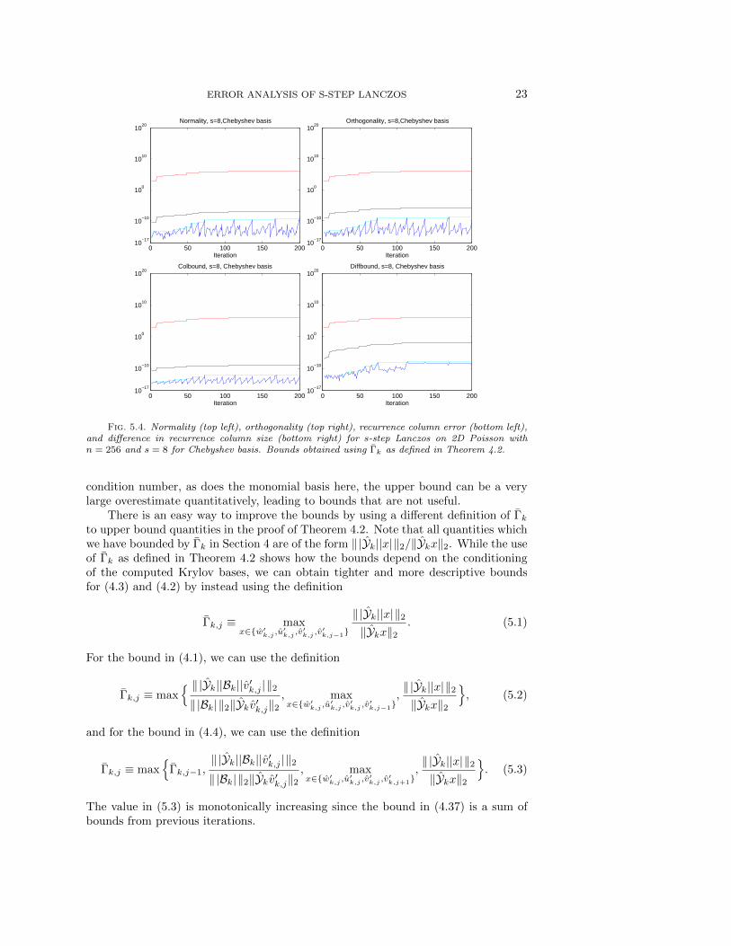
Fig. 5.4. Normality (top left), orthogonality (top right), recurrence column error (bottom left),and difference in recurrence column size (bottom right) for s-step Lanczos on 2D Poisson withn = 256 and s = 8 for Chebyshev basis. Bounds obtained using Γk as defined in Theorem 4.2.

condition number, as does the monomial basis here, the upper bound can be a verylarge overestimate quantitatively, leading to bounds that are not useful.

There is an easy way to improve the bounds by using a different definition of Γkto upper bound quantities in the proof of Theorem 4.2. Note that all quantities whichwe have bounded by Γk in Section 4 are of the form ‖|Yk||x|‖2/‖Ykx‖2. While the useof Γk as defined in Theorem 4.2 shows how the bounds depend on the conditioningof the computed Krylov bases, we can obtain tighter and more descriptive boundsfor (4.3) and (4.2) by instead using the definition

Γk,j ≡ maxx∈{w′k,j ,u

′k,j ,v

′k,j ,v

′k,j−1}

‖|Yk||x|‖2‖Ykx‖2

. (5.1)

For the bound in (4.1), we can use the definition

Γk,j ≡ max{ ‖|Yk||Bk||v′k,j |‖2‖|Bk|‖2‖Ykv′k,j‖2

, maxx∈{w′k,j ,u

′k,j ,v

′k,j ,v

′k,j−1}

,‖|Yk||x|‖2‖Ykx‖2

}, (5.2)

and for the bound in (4.4), we can use the definition

Γk,j ≡ max{

Γk,j−1,‖|Yk||Bk||v′k,j |‖2‖|Bk|‖2‖Ykv′k,j‖2

, maxx∈{w′k,j ,u

′k,j ,v

′k,j ,v

′k,j+1}

,‖|Yk||x|‖2‖Ykx‖2

}. (5.3)

The value in (5.3) is monotonically increasing since the bound in (4.37) is a sum ofbounds from previous iterations.


0 50 100 150 20010

−17

10−10

100

1010

1020

Normality, s=8,monomial basis

Iteration0 50 100 150 200

10−17

10−10

100

1010

1020

Orthogonality, s=8,monomial basis

Iteration

0 50 100 150 20010

−17

10−10

100

1010

1020

Colbound, s=8,monomial basis

Iteration0 50 100 150 200

10−17

10−10

100

1010

1020

Diffbound, s=8,monomial basis

Iteration

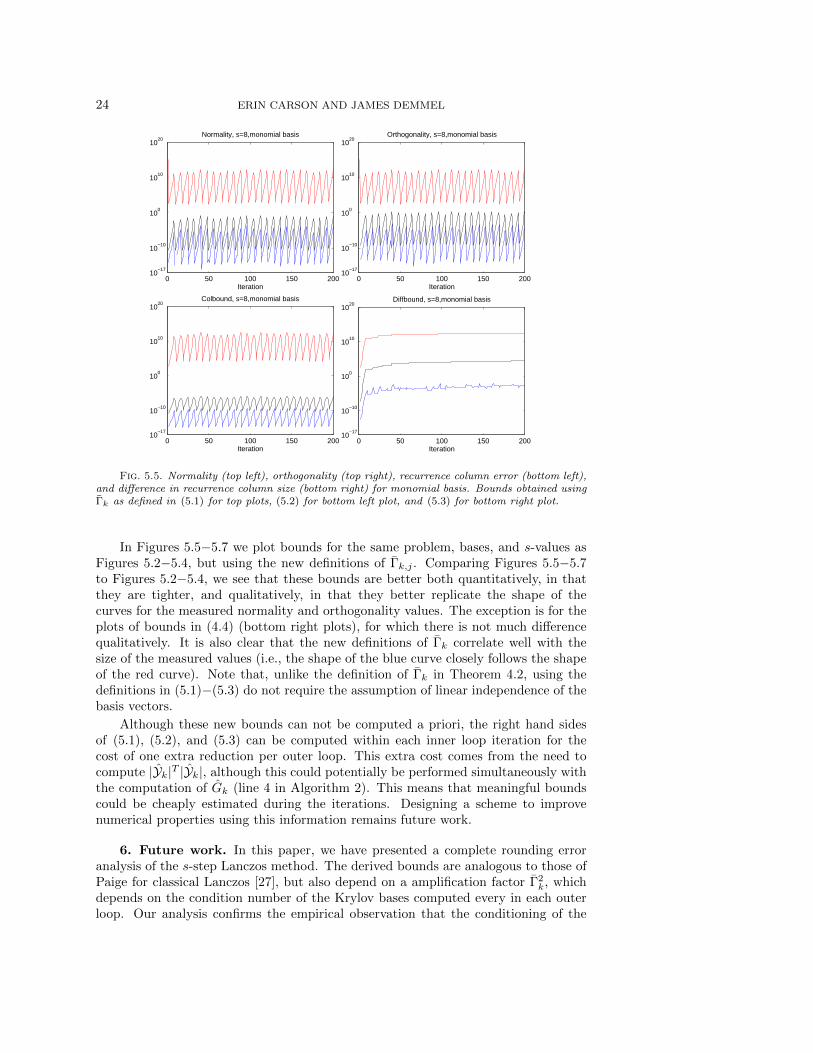
Fig. 5.5. Normality (top left), orthogonality (top right), recurrence column error (bottom left),and difference in recurrence column size (bottom right) for monomial basis. Bounds obtained usingΓk as defined in (5.1) for top plots, (5.2) for bottom left plot, and (5.3) for bottom right plot.

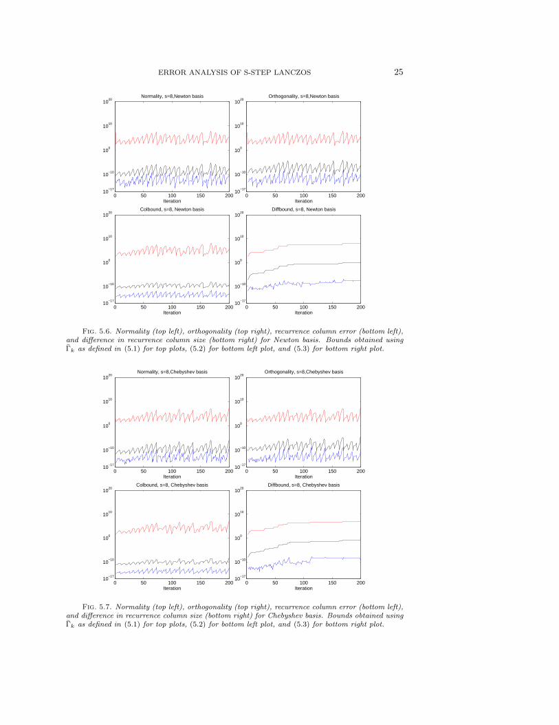
In Figures 5.5−5.7 we plot bounds for the same problem, bases, and s-values asFigures 5.2−5.4, but using the new definitions of Γk,j . Comparing Figures 5.5−5.7to Figures 5.2−5.4, we see that these bounds are better both quantitatively, in thatthey are tighter, and qualitatively, in that they better replicate the shape of thecurves for the measured normality and orthogonality values. The exception is for theplots of bounds in (4.4) (bottom right plots), for which there is not much differencequalitatively. It is also clear that the new definitions of Γk correlate well with thesize of the measured values (i.e., the shape of the blue curve closely follows the shapeof the red curve). Note that, unlike the definition of Γk in Theorem 4.2, using thedefinitions in (5.1)−(5.3) do not require the assumption of linear independence of thebasis vectors.

Although these new bounds can not be computed a priori, the right hand sidesof (5.1), (5.2), and (5.3) can be computed within each inner loop iteration for thecost of one extra reduction per outer loop. This extra cost comes from the need tocompute |Yk|T |Yk|, although this could potentially be performed simultaneously withthe computation of Gk (line 4 in Algorithm 2). This means that meaningful boundscould be cheaply estimated during the iterations. Designing a scheme to improvenumerical properties using this information remains future work.

6. Future work. In this paper, we have presented a complete rounding erroranalysis of the s-step Lanczos method. The derived bounds are analogous to those ofPaige for classical Lanczos [27], but also depend on a amplification factor Γ2

k, whichdepends on the condition number of the Krylov bases computed every in each outerloop. Our analysis confirms the empirical observation that the conditioning of the


0 50 100 150 20010

−17

10−10

100

1010

1020

Normality, s=8,Newton basis

Iteration0 50 100 150 200

10−17

10−10

100

1010

1020

Orthogonality, s=8,Newton basis

Iteration

0 50 100 150 20010

−17

10−10

100

1010

1020

Colbound, s=8, Newton basis

Iteration0 50 100 150 200

10−17

10−10

100

1010

1020

Diffbound, s=8, Newton basis

Iteration

Fig. 5.6. Normality (top left), orthogonality (top right), recurrence column error (bottom left),and difference in recurrence column size (bottom right) for Newton basis. Bounds obtained usingΓk as defined in (5.1) for top plots, (5.2) for bottom left plot, and (5.3) for bottom right plot.

0 50 100 150 20010

−17

10−10

100

1010

1020

Normality, s=8,Chebyshev basis

Iteration0 50 100 150 200

10−17

10−10

100

1010

1020

Orthogonality, s=8,Chebyshev basis

Iteration

0 50 100 150 20010

−17

10−10

100

1010

1020

Colbound, s=8, Chebyshev basis

Iteration0 50 100 150 200

10−17

10−10

100

1010

1020

Diffbound, s=8, Chebyshev basis

Iteration

Fig. 5.7. Normality (top left), orthogonality (top right), recurrence column error (bottom left),and difference in recurrence column size (bottom right) for Chebyshev basis. Bounds obtained usingΓk as defined in (5.1) for top plots, (5.2) for bottom left plot, and (5.3) for bottom right plot.


Krylov bases plays a large role in determining finite precision behavior.

The next step is to extend the analogous subsequent analyses of Paige, in whichhe proves properties about Ritz vectors and Ritz values, relates the convergence ofa Ritz pair to loss of orthogonality, and, more recently, proves a type of augmentedbackward stability for the classical Lanczos method [28, 29].

Another area of interest is the development of practical techniques for improvings-step Lanczos based on our results. This could include strategies for reorthogonal-izing the Lanczos vectors, (re)orthogonalizing the generated Krylov basis vectors, orcontrolling the basis conditioning in a number of ways. The bounds could also be usedfor guiding the use of extended precision in s-step Krylov methods; for example, if wewant the bounds in Theorem 4.2 for the s-step method with precision ε to be similarto those for the classical method with precision ε, one must use precision ε ≈ ε/Γ2

k.

In this analysis, our upper bounds are likely large overestimates. This is in partdue to our replacing Γk with Γ2

k in order to simplify many of the bounds. If theanalysis in this paper is performed instead keeping both Γk and Γ2

k terms, it can beshown that increasing the precision in a few computations (involving the constructionand application of the Gram matrix Gk) can improve the error bounds in Theorem 4.2by a factor of Γk. This motivates the development of mixed precision s-step Lanczosmethods, which could potentially trade bandwidth (in extra bits of precision) forfewer total iterations. As demonstrated in Section 5, it is also possible to use a tighter,iteratively updated bound for Γk which results in tighter and more descriptive boundsfor the quantities in Theorem 4.2.

Acknowledgements. Research is supported by DOE grants DE-SC0004938,DE-SC0005136, DE-SC0003959, DE-SC0008700, DE-FC02-06-ER25786, and AC02-05CH11231, DARPA grant HR0011-12-2-0016, as well as contributions from Intel,Oracle, and MathWorks.

REFERENCES

[1] Z. Bai, D. Hu, and L. Reichel, A Newton basis GMRES implementation, IMA J. Numer.Anal., 14 (1994), pp. 563–581.

[2] G. Ballard, E. Carson, J. Demmel, M. Hoemmen, N. Knight, and O. Schwartz, Commu-nication lower bounds and optimal algorithms for numerical linear algebra, Acta Numer.(in press), (2014).

[3] E. Carson and J. Demmel, A residual replacement strategy for improving the maximumattainable accuracy of s-step Krylov subspace methods, SIAM J. Matrix Anal. Appl., 35(2014), pp. 22–43.

[4] E. Carson, N. Knight, and J. Demmel, Avoiding communication in nonsymmetric Lanczos-based Krylov subspace methods, SIAM J. Sci. Comp., 35 (2013).

[5] A. Chronopoulos and C. Gear, On the efficient implementation of preconditioned s-stepconjugate gradient methods on multiprocessors with memory hierarchy, Parallel Comput.,11 (1989), pp. 37–53.

[6] , s-step iterative methods for symmetric linear systems, J. Comput. Appl. Math, 25(1989), pp. 153–168.

[7] A. Chronopoulos and C. Swanson, Parallel iterative s-step methods for unsymmetric linearsystems, Parallel Comput., 22 (1996), pp. 623–641.

[8] E. de Sturler, A performance model for Krylov subspace methods on mesh-based parallelcomputers, Parallel Comput., 22 (1996), pp. 57–74.

[9] J. Demmel, M. Hoemmen, M. Mohiyuddin, and K. Yelick, Avoiding communication in com-puting Krylov subspaces, Tech. Report UCB/EECS-2007-123, EECS Dept., U.C. Berkeley,Oct 2007.

[10] D. Gannon and J. Van Rosendale, On the impact of communication complexity on the designof parallel numerical algorithms, Trans. Comput., 100 (1984), pp. 1180–1194.

[11] G. Golub and C. Van Loan, Matrix computations, JHU Press, Baltimore, MD, 3 ed., 1996.


[12] A. Greenbaum and Z. Strakos, Predicting the behavior of finite precision Lanczos and con-jugate gradient computations, SIAM J. Matrix Anal. Appl., 13 (1992), pp. 121–137.

[13] M. Gustafsson, J. Demmel, and S. Holmgren, Numerical evaluation of the communication-avoiding Lanczos algorithm, Tech. Report ISSN 1404-3203/2012-001, Department of Infor-mation Technology, Uppsala University, Feb. 2012.

[14] M. Gutknecht, Lanczos-type solvers for nonsymmetric linear systems of equations, ActaNumer., 6 (1997), pp. 271–398.

[15] M. Gutknecht and Z. Strakos, Accuracy of two three-term and three two-term recurrencesfor Krylov space solvers, SIAM J. Matrix Anal. Appl., 22 (2000), pp. 213–229.

[16] A. Hindmarsh and H. Walker, Note on a Householder implementation of the GMRESmethod, Tech. Report UCID-20899, Lawrence Livermore National Lab., CA., 1986.

[17] M. Hoemmen, Communication-avoiding Krylov subspace methods, PhD thesis, EECS Dept.,U.C. Berkeley, 2010.

[18] W. Joubert and G. Carey, Parallelizable restarted iterative methods for nonsymmetric linearsystems. Part I: theory, Int. J. Comput. Math., 44 (1992), pp. 243–267.

[19] S. Kim and A. Chronopoulos, A class of Lanczos-like algorithms implemented on parallelcomputers, Parallel Comput., 17 (1991), pp. 763–778.

[20] , An efficient nonsymmetric Lanczos method on parallel vector computers, J. Comput.Appl. Math., 42 (1992), pp. 357–374.

[21] C. Lanczos, An iteration method for the solution of the eigenvalue problem of linear differentialand integral operators1, J. Res. Natn. Bur. Stand., 45 (1950), pp. 255–282.

[22] G. Meurant, The Lanczos and conjugate gradient algorithms: from theory to finite precisioncomputations, SIAM, 2006.

[23] G. Meurant and Z. Strakos, The Lanczos and conjugate gradient algorithms in finite pre-cision arithmetic, Acta Numer., 15 (2006), pp. 471–542.

[24] M. Mohiyuddin, M. Hoemmen, J. Demmel, and K. Yelick, Minimizing communication insparse matrix solvers, in Proc. ACM/IEEE Conference on Supercomputing, 2009.

[25] C. Paige, The computation of eigenvalues and eigenvectors of very large sparse matrices, PhDthesis, London University, London, UK, 1971.

[26] , Computational variants of the Lanczos method for the eigenproblem, IMA J. Appl.Math., 10 (1972), pp. 373–381.

[27] , Error analysis of the Lanczos algorithm for tridiagonalizing a symmetric matrix, IMAJ. Appl. Math., 18 (1976), pp. 341–349.

[28] , Accuracy and effectiveness of the Lanczos algorithm for the symmetric eigenproblem,Linear Algebra Appl., 34 (1980), pp. 235–258.

[29] , An augmented stability result for the Lanczos hermitian matrix tridiagonalization pro-cess, SIAM J. Matrix Anal. Appl., 31 (2010), pp. 2347–2359.

[30] B. Parlett and D. Scott, The Lanczos algorithm with selective orthogonalization, Math.Comput., 33 (1979), pp. 217–238.

[31] B. Philippe and L. Reichel, On the generation of Krylov subspace bases, Appl. Numer. Math,62 (2012), pp. 1171–1186.

[32] H. Simon, The Lanczos algorithm with partial reorthogonalization, Math. Comput., 42 (1984),pp. 115–142.

[33] S. Toledo, Quantitative performance modeling of scientific computations and creating localityin numerical algorithms, PhD thesis, MIT, 1995.

[34] H. Van der Vorst and Q. Ye, Residual replacement strategies for Krylov subspace iterativemethods for the convergence of true residuals, SIAM J. Sci. Comput., 22 (1999), pp. 835–852.

[35] J. Van Rosendale, Minimizing inner product data dependencies in conjugate gradient itera-tion, Tech. Report 172178, ICASE-NASA, 1983.

[36] H. Walker, Implementation of the GMRES method using Householder transformations, SIAMJ. Sci. Stat. Comput., 9 (1988), pp. 152–163.

[37] W. Wulling, On stabilization and convergence of clustered Ritz values in the Lanczos method,SIAM J. Matrix Anal. Appl., 27 (2005), pp. 891–908.

[38] J. Zemke, Krylov subspace methods in finite precision: a unified approach, PhD thesis, Tech-nische Universitat Hamburg-Harburg, 2003.

Date post:	17-Jul-2018
Category:	Documents
Upload:	dobao
View:	221 times
Download:	0 times

Error analysis of the s-step Lanczos method in finite ... · ERROR ANALYSIS OF THE S-STEP LANCZOS...

Documents