ERROR ESTIMATES FOR GAUSSIAN BEAM SUPERPOSITIONS December 8, 2011 HAILIANG LIU * , OLOF RUNBORG † , AND NICOLAY M. TANUSHEV ‡ Abstract. Gaussian beams are asymptotically valid high frequency solutions to hyperbolic partial differential equations, concentrated on a single curve through the physical domain. They can also be extended to some dispersive wave equations, such as the Schr¨ odinger equation. Superpositions of Gaussian beams provide a powerful tool to generate more general high frequency solutions that are not necessarily concentrated on a single curve. This work is concerned with the accuracy of Gaussian beam superpositions in terms of the wavelength ε. We present a systematic construction of Gaussian beam superpositions for all strictly hyperbolic and Schr¨ odinger equations subject to highly oscillatory initial data of the form Ae iΦ/ε . Through a careful estimate of an oscillatory integral operator, we prove that the k-th order Gaussian beam superposition converges to the original wave field at a rate proportional to ε k/2 in the appropriate norm dictated by the well-posedness estimate. In particular, we prove that the Gaussian beam superposition converges at this rate for the acoustic wave equation in the standard, ε-scaled, energy norm and for the Schr¨ odinger equation in the L 2 norm. The obtained results are valid for any number of spatial dimensions and are unaffected by the presence of caustics. We present a numerical study of convergence for the constant coefficient acoustic wave equation in R 2 to analyze the sharpness of the theoretical results. Key words. high-frequency wave propagation, error estimates, Gaussian beams AMS subject classifications. 58J45, 35L05, 35A35, 41A60, 35L30 1. Introduction. In simulations of high frequency wave propagation, a large number of grid points is needed to resolve and maintain an accurate in time represen- tation of the wave field. Consequently, in this regime, direct numerical simulations are computationally expensive and at sufficiently high frequencies, such simulations are no longer feasible. To circumvent this difficulty, approximate high frequency asymp- totically valid methods are often used. One such popular approach is geometrical optics [7, 33], which is obtained in the limit when the frequency tends to infinity. This method is also known as the WKB method or ray-tracing. The solution of the partial differential equation (PDE) is assumed to be of the form a(t,y,ε)e iφ(t,y)/ε , (1.1) where 1/ε is the large high frequency parameter, φ is the phase, and a is the amplitude of the solution having the Debye expansion in terms of ε, a(t,y,ε)= ∑ N j=0 ε j a j (t,y). The phase and amplitudes a j are independent of the frequency and vary on a much coarser scale than the full wave solution. They can therefore be computed at a compu- tational cost independent of the frequency. However, the geometrical optics approxi- mation breaks down at caustics, where rays concentrate and the predicted amplitude is unbounded [24, 19]. The consideration of difficulties caused by caustics, beginning with Keller in [16] and Maslov and Fedoriuk (see [25]), led to the development of the theory of Fourier integral operators, e.g., as given by H¨ ormander in [10]. Gaussian beams form another high frequency asymptotic model which is closely related to geometrical optics. However, unlike geometrical optics, Gaussian beams * Department of Mathematics, Iowa State University, Ames, IA 50011, USA. ([email protected]). † Department of Numerical Analysis, CSC, KTH, 100 44 Stockholm, Sweden and Swedish e-Science Research Center (SeRC), KTH, 100 44 Stockholm, Sweden. ([email protected]). ‡ Department of Mathematics, The University of Texas at Austin, 1 University Station, C1200, Austin, TX 78712, USA. ([email protected]). 1
Transcript
ERROR ESTIMATES FOR GAUSSIAN BEAM SUPERPOSITIONS
December 8, 2011
HAILIANG LIU∗, OLOF RUNBORG† , AND NICOLAY M. TANUSHEV‡
Abstract. Gaussian beams are asymptotically valid high frequency solutions to hyperbolicpartial differential equations, concentrated on a single curve through the physical domain. They canalso be extended to some dispersive wave equations, such as the Schrodinger equation. Superpositionsof Gaussian beams provide a powerful tool to generate more general high frequency solutions thatare not necessarily concentrated on a single curve. This work is concerned with the accuracy ofGaussian beam superpositions in terms of the wavelength ε. We present a systematic construction ofGaussian beam superpositions for all strictly hyperbolic and Schrodinger equations subject to highlyoscillatory initial data of the form AeiΦ/ε. Through a careful estimate of an oscillatory integraloperator, we prove that the k-th order Gaussian beam superposition converges to the original wavefield at a rate proportional to εk/2 in the appropriate norm dictated by the well-posedness estimate.In particular, we prove that the Gaussian beam superposition converges at this rate for the acousticwave equation in the standard, ε-scaled, energy norm and for the Schrodinger equation in the L2
norm. The obtained results are valid for any number of spatial dimensions and are unaffected bythe presence of caustics. We present a numerical study of convergence for the constant coefficientacoustic wave equation in R
2 to analyze the sharpness of the theoretical results.
1. Introduction. In simulations of high frequency wave propagation, a largenumber of grid points is needed to resolve and maintain an accurate in time represen-tation of the wave field. Consequently, in this regime, direct numerical simulations arecomputationally expensive and at sufficiently high frequencies, such simulations areno longer feasible. To circumvent this difficulty, approximate high frequency asymp-totically valid methods are often used. One such popular approach is geometricaloptics [7, 33], which is obtained in the limit when the frequency tends to infinity.This method is also known as the WKB method or ray-tracing. The solution of thepartial differential equation (PDE) is assumed to be of the form
a(t, y, ε)eiφ(t,y)/ε, (1.1)
where 1/ε is the large high frequency parameter, φ is the phase, and a is the amplitude
of the solution having the Debye expansion in terms of ε, a(t, y, ε) =∑Nj=0 ε
jaj(t, y).The phase and amplitudes aj are independent of the frequency and vary on a muchcoarser scale than the full wave solution. They can therefore be computed at a compu-tational cost independent of the frequency. However, the geometrical optics approxi-mation breaks down at caustics, where rays concentrate and the predicted amplitudeis unbounded [24, 19]. The consideration of difficulties caused by caustics, beginningwith Keller in [16] and Maslov and Fedoriuk (see [25]), led to the development of thetheory of Fourier integral operators, e.g., as given by Hormander in [10].
Gaussian beams form another high frequency asymptotic model which is closelyrelated to geometrical optics. However, unlike geometrical optics, Gaussian beams
∗Department of Mathematics, Iowa State University, Ames, IA 50011, USA. ([email protected]).†Department of Numerical Analysis, CSC, KTH, 100 44 Stockholm, Sweden and Swedish e-Science
Research Center (SeRC), KTH, 100 44 Stockholm, Sweden. ([email protected]).‡Department of Mathematics, The University of Texas at Austin, 1 University Station, C1200,
are defined for all t. For Gaussian beams, the solution is also assumed to be ofthe geometrical optics form (1.1), but a Gaussian beam is a localized solution thatconcentrates near a single ray of geometrical optics in space-time. Although thephase function is real-valued along the central ray, Gaussian beams have a complex-valued phase function off their central ray. The imaginary part of the phase is chosensuch that the solution decays exponentially away from the central ray, maintaining aGaussian-shaped profile. To form a Gaussian beam solution, we first pick a ray andsolve a system of ordinary differential equations (ODEs) along it to find the valuesof the phase, its first and second order derivatives and the amplitude on the ray. Todefine the phase and amplitude away from this ray to all of space-time, we extendthem using a Taylor expansion. Heuristically speaking, along each ray we propagateinformation about the phase and amplitude and their derivatives that allows us toreconstruct the wave field locally in a Gaussian envelope. The existence of Gaussianbeam solutions has been known since sometime in the 1960’s, first in connection withlasers, see Babic and Buldyrev [2]. Later, they were used in the analysis of propagationof singularities in partial differential equations by Hormander [11] and Ralston [30].
In this article, we are interested in the accuracy of Gaussian beam solutions tom-th order linear, strictly hyperbolic PDEs with highly oscillatory initial data of thetype
Pu = 0, (t, y) ∈ (0, T ] × Rn, (1.2)
∂ℓtu(0, y) = ε−ℓN∑
j=0
εjAℓ,j(y)eiΦ(y)/ε , ℓ = 0, . . . ,m− 1 ,
where the strictly hyperbolic operator, P , is defined in Section 2.1, the real valuedphase, Φ(y) belongs to C∞(K0; R) for some compact set K0 ⊂ Rn, and the complexvalued amplitudes, Aℓ,j(y) belong to C∞
0 (K0; C). Furthermore, we will assume that|∇Φ(y)| is bounded away from zero on K0. As a special case, we include the acousticwave equation,
utt − c(y)2∆u = 0, (t, y) ∈ (0, T ]× Rn ,
u(0, y) =
N∑
j=0
εjA0,j(y)eiΦ(y)/ε , and ut(0, y) =
1
ε
N∑
j=0
εjA1,j(y)eiΦ(y)/ε . (1.3)
We also treat the dispersive Schrodinger equation,
− iεut −ε2
2∆u+ V (y)u = 0, (t, y) ∈ (0, T ]× R
n, (1.4)
u(0, y) =
N∑
j=0
εjAj(y)eiΦ(y)/ε .
As above, we will assume that Φ ∈ C∞(K0; R) and Aj ∈ C∞0 (K0; C). Furthermore,
we assume the potential V (y) is smooth and bounded along with all its derivatives,∂βy V ∈ C∞
b (Rn) for all β. For the Schrodinger equation the Hamiltonian is smooth inp (see Section 2.3) and there is no need to assume the bound on |∇Φ| that is necessaryfor strictly hyperbolic equations.
Since these partial differential equations are linear, it is a natural extension toconsider sums of Gaussian beams to represent more general high frequency solutions
ERROR ESTIMATES FOR GAUSSIAN BEAM SUPERPOSITIONS 3
that are not necessarily concentrated on a single ray. This idea was first introduced byBabic and Pankratova in [3] and was later proposed as a method for wave propagationby Popov in [28]. The sum, or rather the integral superposition, of Gaussian beamsin the simplest first order form can be written as
uGB(t, y) =
(
1
2πε
)n2∫
K0
a(t; z)eiφ(t,y−x(t;z);z)/εdz , (1.5)
where K0 is a compact subset of Rn and the phase that defines the Gaussian beam isgiven by
φ(t, y; z) = φ0(t; z) + y · p(t; z) + y · 1
2M(t; z)y . (1.6)
The real vector p(t; z) is the direction of wave propagation and the matrixM(t; z) has apositive definite imaginary part and it gives Gaussian beams their profile. Extensionsof the above superposition are possible in several directions, including using higherorder Gaussian beams in the superposition and using a sum of several superpositionsto approximate the different modes of wave propagation. Higher order Gaussianbeams are created by using an asymptotic series for the amplitude and using higherorder Taylor expansions to define the phase and the amplitude functions, see (2.12)and (2.13). Also, for higher order beams, a cutoff function (2.9) is necessary toavoid spurious growth away from the central ray. Superpositions with higher orderGaussian beams have an improved asymptotic convergence rate. For m-th orderstrictly hyperbolic PDEs, we approximate the solution to the initial value problem bysuperpositions containing beams corresponding to the m families of bicharacteristics.
Accuracy studies for a Gaussian beam solution uGB have traditionally focused onhow well it asymptotically satisfies the PDE, i.e. the size of the norm of PuGB interms of ε. The question of determining the error of the Gaussian beam superpositioncompared to the exact solution was thought to be a rather difficult problem decadesago, see the conclusion section of the review article by Babic and Popov [4]. How-ever, some progress on estimates of the error has been made in the past few years.This accuracy study was initiated by Tanushev in [34], where a convergence rate wasobtained for the initial data. Some earlier results on this were also established byKlimes in [18]. The part of the error that is due to the Taylor expansion off thecentral ray was considered by Motamed and Runborg in [27] for the Helmholtz equa-tion. Liu and Ralston [22, 23] gave rigorous convergence rates in terms of ε for theacoustic wave equation in the scaled energy norm and for the Schrodinger equation inthe L2 norm. However, the error estimates they obtained depend on the number ofspace dimensions in the presence of caustics, since the projected Hamiltonian flow tophysical space becomes singular at caustics. The superpositions in (1.5) can also beinterpreted as a superposition over a phase space submanifold confined in a domainmoving with the Hamiltonian flow, as shown in [22, 23]. A different approach is tocarry out the superpositions in the full phase space and replace the integration in zby integration in (z, p). This was proposed in [20, 21], where initial data was preparedby the Fourier-Bros-Iaglonitzer (FBI) transform. In that case the Hamiltonian flowis regular and there are no caustics, so one expects to obtain a dimensionally inde-pendent error estimate. This has been confirmed for the wave equation by Bougacha,Akian and Alexandre in [5]. A similar result on the Herman-Kluk propagator for theSchrodinger equation was proved by Rousse and Swart [31, 32]. From a computationalstand point, superposition over full phase space generally involves more work thansuperposition over a compact manifold in phase space or in physical space.
4 H. LIU, O. RUNBORG AND N. M. TANUSHEV
Building upon these recent advances, together with an application of a non-squeezing argument proved in Lemma 3.3, we are able to provide a definite answer tothe question of accuracy for Gaussian beam superposition solutions. More precisely,we obtain dimensionally independent estimates for the superposition in physical spacefor general m-th order strictly hyperbolic PDEs and the Schrodinger equation. Ourmain result is the following theorem.
Theorem 1.1. Let u be the exact solution to the PDEs considered, (1.2), (1.3)and (1.4), under the stated assumptions on initial data and partial differential oper-ators. Moreover, let uk be the corresponding k-th order Gaussian beam superpositiongiven in Section 2.2 and Section 2.3, with a sufficiently small cutoff parameter η whenk > 1. We then have the following estimates. For the m-th order strictly hyperbolicPDE (1.2),
εm−1m−1∑
ℓ=0
∥
∥∂ℓt [u(t, ·) − uk(t, ·)]∥
∥
Hm−ℓ−1 ≤ C(T )εk/2 .
For the acoustic wave equation (1.3),
||u(t, ·) − uk(t, ·)||E ≤ C(T )εk/2 ,
where || · ||E is the scaled energy norm (3.2). Finally, for the Schrodinger equation(1.4),
||u(t, ·) − uk(t, ·)||L2 ≤ C(T )εk/2 .
This improves on the results in [22, 23] where the last two error estimates were alsoproved, but with an additional factor ε−γ in the right hand side, where γ = (n− 1)/4for the wave equation and γ = n/4 for the Schrodinger equation. Note that therescaling by εm−1 in the first estimate is convenient here, since it exactly balancesthe rate at which the corresponding norm of the initial data for the PDE (1.2) goesto infinity as ε→ 0.
At present there is considerable interest in using numerical methods based onsuperpositions of beams to resolve high frequency waves near caustics, which beganin the 1980’s with numerical methods for wave propagation in [28, 15, 6] and morespecifically in geophysical applications in [17, 8, 9]. Recent work in this directionincludes simulations of gravity waves [36], of the semiclassical Schrodinger equation[14, 20], and of acoustic wave equations [26, 34]. Numerical techniques based onboth Lagrangian and Eulerian formulations of the problem have been devised [14,21, 20, 26]. A numerical approach for general high frequency initial data closelyrelated to the FBI transform, but avoiding the cost of superposing over all of phasespace, is presented in [29] for the Schrodinger equation. Numerical approaches fortreating general high frequency initial data for superposition over physical space wereconsidered in [35, 1] for the wave equation. Our theoretical results show that thenumerical solutions found in these papers will be accurate when ε≪ 1.
To test the sharpness of the theoretical convergence rates, we present a shortnumerical study in the case of the acoustic wave equation with constant sound speed.Our numerical results indicate that the theoretical rates are sharp for even order k,but similar to the result in [27], we observe a gain in the convergence rate of a factorof ε1/2 for beams of odd order k, which suggests that the actual convergence rate isO(ε⌈k/2⌉).
ERROR ESTIMATES FOR GAUSSIAN BEAM SUPERPOSITIONS 5
This paper is organized as follows: Section 2 introduces Gaussian beams andtheir superpositions for m-th order strictly hyperbolic equations. Furthermore, weconstruct Gaussian beams for the Schrodinger equation. Section 3 is devoted toerror estimates for Gaussian beam superpositions. Detailed norm estimates of theoscillatory operators used in obtaining the error estimates are given in Section 4.Numerical validation of our results is finally presented in Section 5.
2. Construction of Gaussian Beams. In this section, we outline the construc-tion of Gaussian beam superpositions for strictly hyperbolic PDEs. We also constructGaussian beams for the Schrodinger equation.
2.1. Hyperbolic Equations. Let P = Pm + L be a linear strictly hyperbolicm-th order partial differential operator (PDO) in n dimensions with
Pm = ∂mt +
m−1∑
j=0
∑
|β|=m−jgβ(t, y)∂
βy
∂jt , (2.1)
and L a differential operator of order m− 1. The principal symbol of P , denoted byσm(t, y, τ, p), is defined by the formal relationship Pm = σm(t, y,−i∂t,−i∂y). Follow-ing [13, 30], we make the assumptions:
(H1) The coefficients gβ(t, y) are smooth functions, bounded in t and y along withall their derivatives, ∂ℓt∂
αy gβ ∈ C∞
b (Rn) for all ℓ, α.(H2) For |p| 6= 0, the principal symbol σm(t, y, τ, p) has m distinct real roots, when
it is considered as a polynomial in τ .(H3) These roots are uniformly simple in the sense that
∣
∣
∣
∣
∂σm(t, y, τ, p)
∂τ
∣
∣
∣
∣
≥ c0|p|m−1 whenever σm(t, y, τ, p) = 0. (2.2)
We now consider a null bicharacteristic (t(s), x(s), τ(s), p(s)) associated with the prin-cipal symbol σm, defined by the Hamiltonian system of ODEs:
t =∂σm∂τ
, x =∂σm∂p
, τ = −∂σm∂t
, p = −∂σm∂y
, (2.3)
and initial conditions (t(0), x(0), τ(0), p(0)) such that σm(t(0), x(0), τ(0), p(0)) = 0,with p(0) 6= 0. Note that for fixed t(0), x(0) and p(0), we have m distinct choicesfor τ(0), equal to the m distinct real roots of σm(t(0), x(0), τ, p(0)). These choices forτ(0) give m distinct waves that travel in different directions. The curve (t(s), x(s)) inphysical space is the space-time ray that Gaussian beams are concentrated near. Fora proof that the Gaussian beam construction is only possible near this ray, we referthe reader to [30].
The following lemma shows that changing variables s → t in the ODEs above isalways allowed, and also that p(s) remains non-zero if p(0) 6= 0.
Lemma 2.1. Let (t(s), x(s), τ(s), p(s)) be a null bicharacteristic of the Hamil-tonian flow (2.3) with initial data such that |p(0)| 6= 0, σm(t(0), x(0), τ(0), p(0)) = 0and t(0) > 0. Then |p(s)| 6= 0 and t(s) > 0 for all s ≥ 0. Moreover, t(s) → ∞ ass→ ∞.
Proof. We first show that for any fixed (t, y) with (H1) satisfied, the relationσm(t, x, τ, p) = 0 ensures that
|τ | ≤ C|p| (2.4)
6 H. LIU, O. RUNBORG AND N. M. TANUSHEV
for some constant C > 0. This is obviously true if τ = 0. When τ 6= 0, let ξ = p/τ ,we observe that, by homogeneity,
0 = σm(t, y, τ, p) = τmσm(t, y, 1, ξ).
Hence ξ is a root of the polynomial equation
1 +
m∑
|β|=1
gβ(t, y)ξβ = 0 .
Since the coefficients gβ(t, y) are bounded by (H1) it follows that there is a constantsuch that |ξ| ≥ C > 0, which proves (2.4). Note that σm is preserved along theHamiltonian flow (2.3); we have
σm(t(s), x(s), τ(s), p(s)) = 0
by the assumption σm(0) = 0. Hence, |τ(s)| ≤ C|p(s)| for all s.From |p(0)| 6= 0 and the ODE p = −∂σm
∂y it follows that there exists s0 > 0 such
that |p(s)| 6= 0 for s ∈ [0, s0]. For any s when |p(s)| 6= 0 we have |ξ|−1 ≤ C−1, withwhich we can then bound |p| from below as follows:
d
ds|p| = −p · p|p| ≥ −
∣
∣
∣
∣
∣
∣
m−1∑
j=0
∑
|β|=m−j∂ygβ(t, y)p
β
τ j
∣
∣
∣
∣
∣
∣
≥ −Cm−1∑
j=0
∑
|β|=m−j|p||β||τ |j = −C
m−1∑
j=0
∑
|β|=m−j|p|m|ξ|−j ≥ −c1|p|m.
Integration of |p|−m∂s|p| over [0, s] then gives |p(s)| ≥ |p(0)|e−c1s when m = 1, andwhen m > 1,
|p(s)|1−m ≤ |p(0)|1−m + c1(m− 1)s. (2.5)
These two a priori inequalities together with |p(s)| 6= 0 in [0, s0] show that |p(s)| 6= 0for all s ≥ 0. By the strict hyperbolicity (H2), σm(t(s), x(s), τ, p(s)), as a polynomialof τ , has distinct roots and since σm = 0 on the null bicharacteristic, we have thatt(s) = ∂σm/∂τ(s) 6= 0. Continuity and the choice of initial data imply that t(s) > 0for all s ≥ 0. We have left to show that t(s) → ∞. By (H3) and the positivity of t(s),
t(s) − t(0) =
∫ s
0
|t(s′)|ds′ =
∫ s
0
∣
∣
∣
∣
∂σm(t, y, τ, p)
∂τ
∣
∣
∣
∣
ds′ ≥ c0
∫ s
0
|p(s′)|m−1ds′.
Hence, t(s) ≥ t(0) + c0s→ ∞ when m = 1. When m > 1 we use (2.5) above,
t(s) − t(0) ≥∫ s
0
c0|p(0)|1−m + c1(m− 1)s′
ds′ → ∞
when s→ ∞ since the integral is divergent. This proves the lemma.Remark 2.1. Assumptions (H1) and (H2) imply a weaker version of (2.2). The
roots τℓ(t, y, p), ℓ = 0, . . . ,m − 1 of σm(t, y, τ, p) = 0 are positive homogeneous ofdegree one in p. Thus, for η = τ
|p| and ω = p|p| we have
∂σm(t, y, τ, p)
∂τ=
m−1∑
ℓ=0
σmτ − τℓ
= |p|m−1m−1∑
ℓ=0
σm(t, y, η, ω)
η − τℓ(t, y, ω), (2.6)
ERROR ESTIMATES FOR GAUSSIAN BEAM SUPERPOSITIONS 7
which, together with the uniform bound for η by (2.4), yields (2.2) on compact sets in(t, y). In the simple proof above we do, however, need the stronger assumption (H3)(uniformity in (t, y)).
As mentioned above, an immediate consequence of Lemma 2.1 is that we can uset to parametrize the Hamiltonian flow (2.3) instead of s, since the lemma guaranteesthat for a fixed t0 ∈ [0, T ], there exists a unique s0 such that t(s0) = t0. With aslight abuse of notation we will now write x(t) and p(t) for the Hamiltonian flowparametrized by t. Following [30], we define a phase function φ and amplitude func-tions aj via Taylor polynomials. After changing variables s → t in the formulationused in [30] we can write:
φ(t, y) =
k+1∑
|β|=0
1
β!φβ(t)y
β ≡ φ0(t) + y · p(t) + y · 1
2M(t)y +
k+1∑
|β|=3
1
β!φβ(t)yβ ,
aj(t, y) =
k−2j−1∑
|β|=0
1
β!aj,β(t)y
β . (2.7)
We can now define the preliminary k-th order Gaussian beam vk(t, y) as:
vk(t, y) =
⌈k/2⌉−1∑
j=0
εjaj(t, y − x(t))eiφ(t,y−x(t))/ε .
Applying the operator P to this beam and collecting terms containing the same powerof ε, we have
P vk(t, y) =
(
J∑
r=−mεrcr(t, y)
)
eiφ(t,y−x(t))/ε ,
where cr(t, y) are smooth functions independent of ε. The construction in [30] thenproceeds to make cr(t, y) vanishe up to order k− 2(r+m)+ 1 on y = x(t). To obtainthis, (x(t), p(t)) must follow the Hamiltonian flow and the coefficients in the Taylorpolynomials should satisfy ODEs, which are given as follows. By assumption (H2)above, whenever p 6= 0, we can define m Hamiltonians Hℓ(t, x, p) implicitly by therelations σm(t, x,−Hℓ(t, x, p), p) = 0 for ℓ = 0, . . . ,m − 1. For any choice H = Hℓ,the first several ODEs are
x = ∂pH(t, x, p) , p = −∂yH(t, x, p) , (2.8)
φ0 = −H + p · ∂pH(t, x, p) , M = −A−MB −BTM −MCM ,
with
A =∂2H
∂y2, B =
∂2H
∂p∂y, C =
∂2H
∂p2.
By Lemma 2.1 the Hamitonian will be well-defined for all times if p(0) 6= 0. Moreover,we have the following result for the Hessian matrix M(t) of the phase that guaranteesthat the leading order shape of the beam stays Gaussian for all time:
Lemma 2.2 (Ralston ’82, [30]). Suppose that M(0) is chosen so that it has apositive definite imaginary part, M(0)x(0) = p(0), and M(0) = MT(0). Then, for all
8 H. LIU, O. RUNBORG AND N. M. TANUSHEV
t ∈ [0, T ], M(t) will be such that M(t) will have a positive definite imaginary part andM(t) = MT(t).
Before we can fully define a Gaussian beam, one last point needs to be addressed.Since x(t) and p(t) are real, if φ0(0) is real and M(0) chosen as in Lemma 2.2, then theimaginary part of φ(t, y) will be a positive quadratic plus higher order terms aboutx(t). Thus, we must only construct the Gaussian beam in a domain on which thequadratic part is dominant so that ℑφ(t, y) ≥ c|y|2 holds uniformly. To this end, weuse a cutoff function ρη ∈ C∞(Rn; R) with cutoff radius 0 < η ≤ ∞ satisfying,
ρη(z) ≥ 0 and ρη(z) =
1 for |z| ≤ η0 for |z| ≥ 2η
for 0 < η <∞
1 for η = ∞. (2.9)
Now, by choosing η > 0 sufficiently small, we can ensure that on the support ofρη(y − x(t)), ℑφ(t, y − x(t)) > δ|y − x(t)|2 for t ∈ [0, T ]. However, note that for firstorder beams the imaginary part of the phase is quadratic with no higher order terms,so that the cutoff is unnecessary. Thus, to include this case we let the cutoff functionbe defined for η = ∞ by ρ∞ ≡ 1. Nonetheless, we point out that our estimate for firstorder beams remains valid for any 0 < η < ∞. In practical computations one has tobe careful in choosing the appropriate cutoff radius η. We are now ready to finallydefine the k-th order Gaussian beam vk(t, y) as:
vk(t, y) =
⌈k/2⌉−1∑
j=0
εjρη(y − x(t))aj(t, y − x(t))eiφ(t,y−x(t))/ε . (2.10)
2.2. Superpositions of Gaussian Beams. In the previous section, we intro-duced Gaussian beam solutions that satisfy Pu = 0 in an asymptotic sense (see [30]for a precise statement), without too much concern for the values of the solution att = 0. The initial value problem that a single Gaussian beam vk(t, y) approximateshas initial data that is simply given by its values (and the values of its time derivatives)at t = 0. While they resemble the initial conditions for (1.2), they are quite differentsince for example the phase, φ, for vk is complex valued and vk is concentrated in y.
Our goal is to create an asymptotically valid solution to the PDE (1.2), thuswe must also consider the m distinct pieces of initial data given in the form of timederivatives of u at t = 0. To generate solutions based on Gaussian beams thatapproximate the initial data for (1.2), we exploit the linearity properties of P . That is,we use the fact that a linear combination of two Gaussian beams, with different initialparameters, will also be an asymptotic solution to Pu = 0, since each Gaussian beamis itself an asymptotic solution. Building on this idea, we take a family of Gaussianbeams that is indexed by a parameter z ∈ K0, where K0 is the compact subset ofRn discussed in the introduction that contains the support of the amplitudes of theinitial data for (1.2). We will use the notation xℓ(t; z), pℓ(t; z), φℓ(t, y − x(t; z); z),etc, to denote the dependence of these quantities on the indexing parameter z andon the m choices for H(t, x, p) = Hℓ(t, x, p) denoted by ℓ = 0, . . . ,m − 1. Thus, wewill write the k-th order Gaussian beam vk,ℓ(t, y; z). Note that the cutoff radius ηmay vary with z and ℓ between beams, however, as the beam superposition is takenover the compact set K0 and 0 ≤ ℓ ≤ m− 1, there is a minimum value for η that willwork for all beams in the superposition. Thus, we form the k-th order superposition
ERROR ESTIMATES FOR GAUSSIAN BEAM SUPERPOSITIONS 9
solution uk(t, y) as
uk(t, y) =
m−1∑
ℓ=0
(
1
2πε
)n2∫
K0
vk,ℓ(t, y; z)dz , (2.11)
where the phase and amplitude that define the Gaussian beam,
vk,ℓ(t, y; z) =
⌈k/2⌉−1∑
j=0
εjρη(y − xℓ(t; z))aℓ,j(t, y − xℓ(t; z); z)eiφℓ(t,y−xℓ(t;z);z)/ε ,
are given by
φℓ(t, y; z) = φℓ,0(t; z) + y · pℓ(t; z) + y · 1
2Mℓ(t; z)y +
k+1∑
|β|=3
1
β!φℓ,β(t; z)y
β , (2.12)
aℓ,j(t, y; z) =
k−2j−1∑
|β|=0
1
β!aℓ,j,β(t; z)y
β . (2.13)
We remind the reader that each vk,ℓ(t, y; z) requires initial values for the ray and allof the amplitude and phase Taylor coefficients. The appropriate choice of these initialvalues will make uk(0, y) asymptotically converge the initial conditions in (1.2). Thefirst step is to choose the origin of the rays and the initial coefficients of φℓ up toorder k+ 1. Letting the ray begin at a point z and expanding Φ(y) in a Taylor seriesabout this point,
Φ(y) =
k+1∑
|β|=0
1
β!Φβ(z)(y − z)β + error ,
we initialize the ray and Gaussian beam phase associated with τℓ as
Determining the initial coefficients for the amplitudes involves a more complicatedprocedure. As with the phase, we expand all of the amplitude functions in Taylorseries,
Aℓ,j(y) =
k−2j−1∑
|β|=0
1
β!Aℓ,j,β(z)(y − z)β + error .
Next, we look at the time derivatives of uk at t = 0, to the lowest order in ε. We equatethe coefficients of (y − z) to the the corresponding terms in the Taylor expansions ofBℓ,j and recalling that
we obtain the following m×m system of linear equations:
1 · · · 1...
...(iτ0)
ℓ · · · (iτm−1)ℓ
......
(iτ0)m−1 · · · (iτm−1)
m−1
a0,0,β
...aℓ,0,β
...am−1,0,β
=
A0,0,β
...Aℓ,0,β
...Am−1,0,β
.
10 H. LIU, O. RUNBORG AND N. M. TANUSHEV
Since the τℓ are distinct, this Vandermonde matrix is invertible, so the solution willgive the initial coefficients for the first amplitude for each of the m Gaussian beams. Ifwe proceed with the next orders in ε, we would obtain the same m×m linear systemfor [a0,j,β, . . . , am−1,j,β]
T, except that the right hand side will not only depend on theTaylor coefficients Bℓ,j,β, but also on previously computed aℓ,q,γ , q < j, coefficientsand their time derivatives. Thus, all of the necessary initial coefficients for each of them Gaussian beams can be computed sequentially. Summarizing this construction, wehave that at t = 0 and ℓ = 0, . . . ,m− 1,
∂ℓtuk(0, y) =
(
1
2πε
)n2∫
K0
ε−ℓN∑
j=0
εjρη(y − z)bℓ,j(y)eiφ(y)/εdz + O(ε∞) , (2.14)
where φ(y) is the Taylor expansion of Φ(y)+ i|y− z|2/2 to order k+1 and each bℓ,j isthe same as the Taylor expansion of Bℓ,j up to order k − 2j − 1. The O(ε∞) term ispresent because some of the time derivatives fall on the cutoff function ρη(y−xℓ(t; z)).The contributions of such terms decays exponentially as ε → 0, since the derivativesof ρη(y − xℓ(t; z)) are compactly supported and vanish near y = z.
Remark 2.2. For ease of notation and exposition, in (1.2) we have taken thephase Φ to be the same for all of the m initial data, however, this is not a requirement.We can form m different Gaussian beam superpositions that each satisfy one of thesem conditions with a specific phase and the rest with zero initial data. Then, summingthese m solutions we obtain a more general solution of (1.2) with m different phasefunctions for each of initial data piece.
Remark 2.3. In the initialization of Mℓ(0; z) we take its imaginary part to begiven by i Idn×n for simplicity. All of the results in this paper can be carried out if weinstead took the imaginary part to be given by iγ Idn×n, for some constant γ > 0, andadjusted the normalization constant in (2.11) appropriately. However, it is importantto note that the constants throughout this paper will depend on γ and that in general,we expect that increasing γ will increase the evolution error in the Gaussian beamsand that decreasing γ will increase the error in approximating the initial data.
This completes the construction of the Gaussian beam superpositions uk for theinitial value problem (1.2) for general m-th order strictly hyperbolic operators. Fromthis point, we will assume that the parameter η is chosen as η = ∞ for the first ordersuperposition u1 and that for higher order superpositions it is taken small enough (andindependent of z and ℓ) to make ℑφℓ(t, y − xℓ(t; z); z) > δ|y − xℓ(t; z)|2 for t ∈ [0, T ]and y ∈ suppρη(y − xℓ(t; z)). Lemma 3.4 below shows that this is always possible.
2.3. The Schrodinger Equation. The construction of Gaussian beams forhyperbolic equations can be extended to the Schrodinger equation by replacing theoperator P with a semiclassical operator P ε. Then, we can similarly construct asymp-totic solutions to P εu = 0 as ε→ 0. In this section, we briefly review the constructionpresented in [23] for the Schrodinger equation (1.4) with a smooth external potentialV (y). Note that the small parameter ε represents the fast space and time scale intro-duced in the equation, as well as the typical wavelength of oscillations of the initialdata.
We recall that the k-th order Gaussian beam solutions are of the form
vk(t, y; z) =
⌈k/2⌉−1∑
j=0
εjρη(y − x(t; z))aj(t, y − x(t; z); z)eiφ(t,y−x(t;z);z)/ε,
ERROR ESTIMATES FOR GAUSSIAN BEAM SUPERPOSITIONS 11
where the phase and amplitudes are given in (2.12) and (2.13) and ρη is the cutofffunction (2.9). Furthermore, the subindex “ℓ” has been suppressed since for theSchrodinger equation there is only one choice for H(t, x, p), namely
H(t, x, p) =|p|22
+ V (x) . (2.15)
The system (2.8) for the bicharacteristics (x(t; z), p(t; z)) is then given by
x = p , x(0; z) = z ,
p = −∇yV, p(0; z) = ∇yΦ(z) .
The equations for the phase and amplitude Taylor coefficients are derived in thesame way as for the strictly hyperbolic equations. The phase coefficients along thebicharacteristic curve satisfy
have global in time solution, thus vk(t, y; z) is well-defined for all 0 ≤ t ≤ T .The k-th order Gaussian beam superposition is finally formed as
uk(t, y) =
(
1
2πε
)n2∫
K0
vk(t, y; z)dz .
As in the case of strictly hyperbolic PDEs, we will assume that the cutoff parameterη is chosen as η = ∞ for the first order superposition u1 and that for higher ordersuperpositions it is taken small enough (and independent of z) to make ℑφ(t, y −x(t; z); z) > δ|y − x(t; z)|2 for t ∈ [0, T ] and y ∈ suppρη(y − x(t; z)). Again,Lemma 3.4 ensures that this can be done. Furthermore, we note that Remark 2.3concerning the initial choice of the imaginary part of M(0; z) also applies to thesuperposition for the Schrodinger equation.
3. Error Estimates for Gaussian Beams. In this section we prove the asymp-totic convergence results for superpositions of Gaussian beams given in our main re-sult, Theorem 1.1. The corner stone of our error estimates are the well-posednessestimates for each PDE. Since they are crucial to our analysis we summarize themhere.
12 H. LIU, O. RUNBORG AND N. M. TANUSHEV
Theorem 3.1. The generic well-posedness estimate
‖u(t, ·)‖S ≤ ‖u(0, ·)‖S + Cεq∫ t
0
‖Θ[u](τ, ·)‖L2dτ , (3.1)
applies to• the m-th order strictly hyperbolic PDE (1.2) with Θ = P , q = 0 and ‖ · ‖S the
Sobolev space-time norm,
m−1∑
ℓ=0
∥
∥∂ℓtu(t, ·)∥
∥
Hm−ℓ−1 ,
where Hs is the Sobolev s-norm (H0 = L2),• the wave equation (1.3) with Θ = ∂2
t − c(y)2∆, q = 1 and ‖ · ‖S the ε-scaledenergy norm,
||u(t, ·)||E :=
(
ε2
2
∫
Rn
|ut|2c(y)2
+ |∇u|2dy)1/2
, (3.2)
• and the Schrodinger equation (1.4) with Θ = P ε, q = −1 and ‖ · ‖S thestandard L2 norm.
Proof. The results for the wave and Schrodinger equation are standard and canbe found in most books on PDEs. The result for m-th order equations is a bit moretechnical to prove and appears in Section 23.2 of [13] (Lemma 23.2.1).
Remark 3.1. Since the wave equation is a second order strictly hyperbolic PDE,we have two distinct well-posedness estimates in terms of two different norms. Fur-thermore, we note that ‖ · ‖E is only a norm over the class of functions that tend tozero at infinity, which we are considering here.
When Theorem 3.1 is applied to the difference between the Gaussian beam super-position, uk, and the true solution, u, for any one of the PDEs that we are considering,we obtain the following estimate for t ∈ [0, T ],
with the appropriate choices for Θ, q and ‖ · ‖S. We will refer to the first term on theright hand side as the error in approximating the initial data or the initial data errorand to the second term as the evolution error.
Using the ideas in [34], we prove Theorem 3.7, which shows the convergence ratein ε of the Gaussian beam superposition to the initial data for any given Sobolevnorm. Thus, this theorem extends a result of [34], so that we can use it to estimatethe initial data error in the more general well-posedness estimates above.
The evolution error has been estimated in the work of previous authors [22, 23, 5,32]. The necessary steps used by those authors are quite general and can be appliedto any strictly hyperbolic equation as well as any linear dispersive wave equation aslong as it is semi-classically rescaled. Following these ideas, we show in Lemma 3.5that for all of the PDEs that we consider, Θ[uk] can be written in the form
ERROR ESTIMATES FOR GAUSSIAN BEAM SUPERPOSITIONS 13
so that the key to estimating the evolution error is precise norm estimates in terms ofε of the oscillatory integral operators Qαj ,gj ,η : L2(K0) 7→ L∞([0, T ];L2(Rn)), definedas follows. For a fixed t ∈ [0, T ], a multi-index α, a compact set K0 ⊂ Rn, a cutofffunction ρη (2.9) with cutoff radius 0 < η ≤ ∞ and a function g(t, y; z), we let
with the functions g(t, y; z), φ(t, y; z) and x(t; z) satisfying for all t ∈ [0, T ],(A1) x(t; z) ∈ C∞([0, T ] ×K0),(A2) φ(t, y; z), g(t, y; z) ∈ C∞([0, T ]× Rn ×K0),(A3) ∇φ(t, 0; z) is real and there is a constant C such that for all z, z′ ∈ K0,
|∇yφ(t, 0; z) −∇yφ(t, 0; z′)| + |x(t; z) − x(t; z′)| ≥ C|z − z′| ,(A4) for |y| ≤ 2η (or for all y if η = ∞), there exists a constant δ such that for all
z ∈ K0,
ℑφ(t, y; z) ≥ δ|y|2 ,(A5) for any multi-index β, there exists a constant Cβ , such that
supz∈K0
y∈Rn
∣
∣∂βy g(t, y; z)∣
∣ ≤ Cβ .
With this definition, the following norm estimate of Qα,g,η will be proved in Section 4.Theorem 3.2. Under the assumptions (A1)–(A5),
supt∈[0,T ]
‖Qα,g,η‖L2 ≤ C(T ).
This theorem improves the norm estimate of Qα,g,η given in [22, 23], which has anadditional factor ε−γ in the right hand side, with γ = (n−1)/4 for the wave equationand γ = n/4 for the Schrodinger equation. Instead of estimating the integral directly,we follow the arguments in [5, 31] to relate the estimate of the oscillatory integral tothe operator norm, through the use of an adjoint operator. An essential ingredientin estimating the operator norm is the non-squeezing lemma (Lemma 3.3), whichstates that the distance between two physical points is comparable to the distancebetween their Hamiltonian trajectories measured in phase space, even in the presenceof caustics. Using Theorem 3.2 we are able to prove the same convergence rate forGaussian beam superpositions over physical space that is achieved in [5] for beamsuperposition carried out in full phase space. Thus, we improve on the error estimatesgiven in [22, 23] to obtain error estimates for the Gaussian beam superposition thatare independent of dimension as given in Theorem 1.1.
We conclude this section with two remarks.Remark 3.2. The assumption of C∞ smoothness for all functions is made for
simplicity to avoid a too technical discussion about precise regularity requirements. Inthis sense, Theorem 1.1 and Theorem 3.2 can be sharpened, since they will be truealso for less regular functions.
Remark 3.3. If the condition in assumption (A4) is satisfied for all y there isno need for the cutoff function in the definition of the operator Q in (3.5). We treatthis case by taking η = ∞ and defining ρ∞ ≡ 1. The operators with η = ∞ are usedin the case of first order Gaussian beams.
14 H. LIU, O. RUNBORG AND N. M. TANUSHEV
3.1. Gaussian Beam Phase. In this section, we show that the Gaussian beamphase φ given in (2.12) is an admissible phase for the operators Qα,g,η. We beginwith a lemma based on the regularity of the Hamiltonian flow map, St, stating thatthe difference |z − z′| is comparable to the sum |p(t; z)− p(t; z′)| + |x(t; z) − x(t; z′)|.Note, however, that because of caustics it is not true that |z − z′| is related in thisway to either of the individual terms |p(t; z) − p(t; z′)| or |x(t; z) − x(t; z′)|.
Lemma 3.3 (Non-squeezing lemma). Let St be a Hamiltonian flow map,(x(t; z), p(t; z)) = St(x(0; z), p(0; z)), associated to a strictly hyperbolic PDO (2.8)or to the Schrodinger operator (2.15). Let K0 be a compact subset of Rn and as-sume that p(0; z) is Lipschitz continuous in z ∈ K0 for the flow associated with theSchrodinger operator. Additionally, assume that infz∈K0
|p(0; z)| = δ > 0 for theflow associated with the strictly hyperbolic PDO. Under these conditions, there existpositive constants c1 and c2 depending on T and δ, such that
We begin with the flow associated with the Hamiltonian for the Schrodinger operator.Let us introduce the set K0 = (z, p(0; z)) : z ∈ K0 and note that St is invertiblewith inverse S−t and regular for all t so that
supt∈[0,T ]
supZ∈conv(K0)
∥
∥
∥
∥
∥
∂St(Z)
∂Z
∥
∥
∥
∥
∥
≤ C , supt∈[0,T ]
supX∈conv(St(K0))
∥
∥
∥
∥
∥
∂S−t(X)
∂X
∥
∥
∥
∥
∥
≤ C ,
where conv(E) denotes the convex hull of the set E. Now, noting that
X −X ′ =
∫ 1
0
d
dsSt(sZ + (1 − s)Z ′)ds =
∫ 1
0
∂St(sZ + (1 − s)Z ′)
∂Z(Z − Z ′)ds , (3.7)
and taking ℓ1 norms, since sZ + (1 − s)Z ′ ∈ conv(K0), we have
which completes the proof of the lemma for the Hamiltonian flow associated with theSchrodinger operator.
For the flow associated with the strictly hyperbolic operator, we follow the sameidea, but we have to be careful near |p| = 0. Thus, in addition to K0, we introducethe sets
provided that p(s) = (1 − s)p0 + sp′0 satisfies inf0≤s≤1 |p(s)| ≥ δ/2, which guarantees
that sZ + (1 − s)Z ′ ∈ K0 \ Bδ/2 for 0 ≤ s ≤ 1. On the other hand, suppose thatinf0≤s≤1 |p(s)| < δ/2. We define p∗ as the point on the line connecting p0 to p′0 withsmallest norm and let s∗ = argmin0≤s≤1 |p(s)| so that p∗ = p(s∗). Then
which shows that (3.8) holds for all Z, Z ′ ∈ K0. This gives the right half of (3.6).For the left half of (3.6), we note that by Lemma 2.1, inft∈[0,T ],z∈K0
|p(t; z)| ≥ δ > 0,so that we can consider the inverse map S−t in exactly the same way as St above andshow that ||Z − Z ′||1 ≤ C||X −X ′||1. Thus we obtain the left half of (3.6),
We are now ready to show that the phase function for a k-th order Gaussian beamis an admissible phase for the operators Qα,g,η.
Lemma 3.4. Let φ(t, y; z) and x(t; z) be the phase and central ray associatedto a k-th order Gaussian beam for (1.2), (1.3) or (1.4) as given in Section 2.2 andSection 2.3. The rays x(t; z) satisfy (A1) and φ(t, y; z) satisfies assumptions (A2)through (A4) if η is sufficiently small. In the case of k = 1, η can take any value in(0,∞].
Proof. The smoothness assumptions (A1) and (A2) follow from smoothness ofinitial data and smoothness of the coefficients in the underlying PDE. By definition,∇yφ(t, 0; z) = p(t; z) and (A3) follows from the non-squeezing lemma, Lemma 3.3.Finally, since the lower order terms of φ are real,
ℑφ(t, y; z) = y · (ℑM(t; z))y +
k+1∑
|β|=3
1
β!ℑφβ(t; z)yβ .
16 H. LIU, O. RUNBORG AND N. M. TANUSHEV
Recalling that by Lemma 2.2, ℑM(t; z) is positive definite, we therefore have thatwhen |y| ≤ 2η,
ℑφ(t, y; z) ≥ C|y|2 −k+1∑
|β|=3
1
β!‖ℑφβ(t; z)‖L∞|y||β|
≥ C|y|2 − |y|2k+1∑
|β|=3
1
β!‖ℑφβ(t; z)‖L∞(2η)|β|−2
≥ |y|2
C − 2η
k+1∑
|β|=3
1
β!‖ℑφβ(t; z)‖L∞(2η)|β|−3
≥ δ(η)|y|2,
where the constant δ(η) is positive for small enough η and independent of t ∈ [0, T ],since φβ(t; z) are smooth functions of t. This shows that φ(t, y; z) satisfies (A4).When k = 1, there are only quadratic terms in the phase and in this case φ(t, y; z)will satisfy (A4) for any choice of η ∈ (0,∞].
3.2. Representations of P [uk] in Terms of Qα,g,η. In this section, we showthat several of the intermediate quantities in the proof of Theorem 1.1 can be writtenas sums involving the operators Qα,g,η.
Lemma 3.5. Let P be an m-th order strictly hyperbolic operator and P ε asemiclassical Schrodinger operator, satsifying the assumptions stated for (1.2) (inSection 2.1) and (1.4) respectively. Let uk be the corresponding Gaussian beam su-perpositions given in Section 2.2 and Section 2.3. Then P [uk] and P ε[uk] can beexpressed as a finite sum of the operators Q:
P [uk]
P ε[uk]
=
(
1
2π
)n2
J∑
j=1
εℓj(
Qαj ,gj ,η χK0
)
(t, y) + O(ε∞),
ℓj ≥ k/2 −m+ 1
ℓj ≥ k/2 + 1,
with χK0(z) the characteristic function on K0 and Qαj ,gj ,η satisfying assumptions
(A1)-(A5) if η is sufficiently small. In the case of k = 1, η can take any value in(0,∞].
Proof. For a single Gaussian beam vk,ℓ(t, y; z) for the hyperbolic operator, fol-lowing the discussion in [30] and Section 2.1, we have
P [vk,ℓ(t, y; z)] =
⌈k/2⌉−1∑
r=−mεrρη(y − xℓ(t; z))cr,ℓ(t, y; z)e
iφ(t,y−xℓ(t;z);z)/ε + Ek(t, y; z) ,
where Ek contains terms that are multiplied by derivatives of the cutoff function.For first order beams η = ∞ and ρ∞ ≡ 1 making E1(t, y; z) ≡ 0. For higher orderbeams, Ek ≡ 0 in an η neighborhood of xℓ(t; z) and since η is small enough so thatthe imaginary part of φℓ is strictly positive for η ≤ |y − xℓ(t; z)| ≤ 2η, Ek will decayexponentially as ε→ 0. Thus, Ek = O(ε∞) for all orders of beams and t ∈ [0, T ].
Each cr can be expressed in terms of the symbols of P :
ERROR ESTIMATES FOR GAUSSIAN BEAM SUPERPOSITIONS 17
where aℓ,j ≡ 0 for j 6∈ [0, ⌈k/2⌉−1] and L is given by (using the Einstein summation),
La = −i(
∂σm∂pj
(y, ∇φℓ)∂a
∂yj
)
−(
i
2
∂2σm∂pj pq
(y, ∇yφℓ)φℓ,yj yq + σm−1(y, ∇φℓ))
a ,
with ∇ = (∂t,∇), y = (t, y) and p = (τ, p). The function Rℓ,0(t, y; z) ≡ 0 and thefunctions Rℓ,j(t, y; z) for j > 0 are complicated functions of the m−2 and lower ordersymbols of P and the functions φℓ, aℓ,0, . . . , aℓ,j−1 and their derivatives. We note thatsince aℓ,j(t, y; z) are compactly supported in z ∈ K0, so are the functions cr,ℓ(t, y; z).
By the construction of a Gaussian beam, cr,ℓ vanishes up to order k − 2(r +m) + 1on y = xℓ(t; z). Note that k − 2(r +m) + 1 may be negative, in which case, cr,ℓ isnot necessarily 0 on y = xℓ(t; z). Thus, by Taylor’s remainder formula,
cr,ℓ(t, y; z) =∑
|α|=[k−2(r+m)+2]+
cr,ℓ,α(t, y; z) (y − xℓ(t; z))α ,
for some coefficient functions cr,ℓ,α(t, y; z) that are compactly supported in z ∈ K0
and [a]+ = max[a, 0]. For the superposition uk(t, y), we have
modulo additive terms that are O(ε∞) and where χK0(z) is the characteristic function
on K0 and the functions cr,ℓ,α(t, y; z) satisfy condition (A5) since the coefficients ofP , φℓ,β and aℓ,j,β are all smooth. By Lemma 3.4 the operators also satisfy (A1)-(A4)under the condition on η.
To simplify the notation, let j = 1, . . . , J < ∞ enumerate all of the combinationof ℓ, r, and α in the triple sum above and rewrite the sums as
P [uk] =
(
1
2π
)n2
J∑
j=1
εℓj(
Qαj ,gj ,η χK0
)
(t, y) + O(ε∞) ,
with ℓj ≥ (k/2 −m+ 1) and gj = crj,ℓj ,αj . Thus, we have the desired result for P .
18 H. LIU, O. RUNBORG AND N. M. TANUSHEV
Now, for each Gaussian beam vk(t, y; z) for the Schrodinger equation defined inSection 2.3, following [23], we compute
P ε[vk] = ρηPε
⌈k/2⌉−1∑
j=0
εjajeiφ/ε
+ Ek(t, y; z)
where again Ek = O(ε∞). Note that
e−iφ/εP ε[aeiφ/ε] = aG(t, y) − iεLa− ε2
2a ,
with
G = ∂tφ+1
2|∇yφ|2 + V (y) and L = ∂t + ∇yφ · ∇y +
1
2yφ .
Thus, we have
P ε
⌈k/2⌉−1∑
j=0
εjajeiφ/ε
=
⌈k/2⌉−1∑
j=0
εj[
ajG− iεLaj −ε
2yaj
]
eiφ/ε =
⌈k/2⌉+1∑
r=0
εrdreiφ/ε ,
where for convenience aj ≡ 0 for j 6∈ [0, ⌈k/2⌉ − 1] and
dr = arG− iLar−1 −1
2yar−2 , r = 0, . . . , ⌈k/2⌉+ 1 .
By construction of the phase coefficients in Section 2.3, we have that on y = x(t; z), Gvanishes to order k+1 and by construction of the amplitude coefficients, the quantity−iLar−1 − 1
2yar−2 vanishes to order k−2r+1. Thus, dr vanishes to order k−2r+1on y = x(t; z), where again we remark that if k−2r+1 is negative, dr does not vanishon y = x(t; z). By Taylor’s remainder formula, we have
dr(t, y; z) =∑
|α|=[k+2−2r]+
dr,α(t, y; z) (y − x(t; z))α ,
with dr,α(t, y; z) compactly supported in z ∈ K0. Hence,
P ε[vk] = ρη
⌈k/2⌉+1∑
r=0
εr
∑
|α|=[k+2−2r]+
dr,α(y − x(t; z))α
eiφ/ε + O(ε∞) .
For the superposition, we have
P ε[uk] =
(
1
2πε
)n2∫
K0
P ε[vk]dz
=
(
1
2π
)n2
⌈k/2⌉−1∑
r=0
∑
|α|=[k+2−2r]+
εr+|α|/2(Qα,dr,α,ηχK0)(t, y) + O(ε∞) .
As above, the smoothness of V (y), φβ and aj,β guarantees that dr,α satisfies (A5),while Lemma 3.4 ensures that also (A1)-(A4) are true for Qα,dr,α,η under the conditionon η. Again, we let j = 1, . . . , J <∞ enumerate all of the combination of r and α inthe double sum above. Thus,
P ε[uk] =
(
1
2π
)n2
J∑
j=1
εℓj(
Qαj ,gj ,η χK0
)
(t, y) + O(ε∞) ,
with ℓj ≥ (k/2 + 1) and gj = drj ,αj . Thus, the proof is complete.
ERROR ESTIMATES FOR GAUSSIAN BEAM SUPERPOSITIONS 19
3.3. Initial Data Errors. In addition to establishing the role of the Q-operatorsand estimating their norms, we need to consider the convergence of the Gaussian beamsuperposition to the initial data to be able to prove Theorem 1.1. We start with thefollowing lemma.
Lemma 3.6. Let Φ ∈ C∞(K0) be a real-valued function and Aj ∈ C∞0 (K0).
With k ≥ 1, define
u(y) =
N∑
j=0
εjAj(y)eiΦ(y)/ε,
uk(y) =
(
1
2πε
)n2∫
Rn
ρη(y − z)
N∑
j=0
εjaj(y − z; z)eiφ(y−z;z)/ε−|y−z|2/2εdz ,
where φ(y− z; z) is the k+1 order Taylor series of Φ about z, aj(y− z; z) is the sameas the Taylor series of Aj about z up to order k − 2j − 1 (but may differ in higherorder terms) and ρη is the cutoff function (2.9) with 0 < η ≤ ∞. Then for someconstant Cs,
‖uk − u‖Hs ≤ Csεk2−s .
Proof. The proof of this lemma is based on a discussion in [34]. We first assumethat η <∞. Looking at each of the terms in the sum above separately, the estimatedepends on how well
Since we want to estimate the difference between these two functions in a Sobolevnorm, we need to consider differences between their ∂βy derivatives in the L2 norm.Since derivatives of (3.10) that fall on the cutoff function ρη(y− z) vanish in a neigh-borhood of z = y and the integrand is compactly supported in y and z, they will beO(ε∞) in the L2 norm and do not contribute to the estimate. Thus, when we differen-tiate (3.9) and (3.10) by ∂βy and pair the results from the sequence of differentiations,the terms that will contribute to the estimate will be of the form
(
1
2πε
)n2
εj−ℓCγℓℓ ∂δ1y [Aj(y)]
(
ℓ∏
m=1
∂γmy
[
iΦ(y) − |y − z|2/2]
)
(3.11)
for (3.9) and
(
1
2πε
)n2
εj−ℓCγℓℓ ∂δ1y [aj(y − z; z)]
(
ℓ∏
m=1
∂γmy
[
iφ(y − z; z)− |y − z|2/2]
)
(3.12)
for (3.10), where Cγℓℓ are combinatorial coefficients. These terms are integrated
over Rn in z and summed over the multi-indexes δ1 + γ = β, the index ℓ = 1 . . . |γ|,
20 H. LIU, O. RUNBORG AND N. M. TANUSHEV
and multi-indexes |γ1|, . . . , |γℓ| ≥ 1, γ1 + . . . + γℓ = γ. Furthermore, we have thatmaxm[γm] ≤ |γ| − ℓ + 1. These formulas can be obtained through long but straight-forward calculations. The important part is to recall that iφ(y − z; z)− |y − z|2/2 isthe k+1 order Taylor series of iΦ(y)− |y− z|2/2 about z and aj(y− z; z) agrees withthe Taylor series of Aj(y) about z up to order k − 2j − 1, so that (3.12) will agreewith the Taylor series of (3.11) up to order
min
[
k − 2j − 1 − |δ1|, k + 1 − max1≤m≤ℓ
|γm|]
≥ k − 2j − 1 − |δ1| − |γ| + ℓ
= k − 2j − 1 − |β| + ℓ .
Thus, we have that ‖∂βy (uk − u)‖L2 can be estimated by a sum of terms of the form
εj−ℓ
∥
∥
∥
∥
∥
(
1
2πε
)n2∫
Rn
[
Bℓ(y)eiΦ(y)/ε−|y−z|2/2ε
− ρη(y − z)bℓ(y − z; z)eiφ(y−z;z)/ε−|y−z|2/2ε]
dz
∥
∥
∥
∥
∥
L2
, (3.13)
where ℓ ≤ |β|, |Bℓ− bℓ| = O(|y− z|k−2j−|β|+ℓ) and |Φ−φ| = O(|y− z|k+2). Now, theproof of Theorem 2.1 in [34] can be applied directly to (3.13) to obtain the estimate,
‖∂βy (uk − u)‖L2 ≤N∑
j=0
εj−ℓCεk2−j− |β|
2+ ℓ
2 ≤ Cεk2−|β| .
Thus, we have the result for η <∞. The extension for ρ∞ ≡ 1 follows directly, sincethe cutoff ρν for ν <∞ introduces O(ε∞) errors in the L2 norm:
as 1− ρν vanishes in a neighborhood z = y and the integrand is compactly supportedin z.
Using Lemma 3.6, we can estimate the asymptotic convergence rate of the super-position solution to the initial data.
Theorem 3.7. For the Gaussian beam superposition, uk, given in Section 2.2and the solution, u, to the strictly hyperbolic PDE (1.2), we have
∥
∥∂ℓtuk(0, ·) − ∂ℓtu(0, ·)∥
∥
Hs ≤ Cℓ,sεk2−ℓ−s ,
for some constant Cℓ,s and 0 ≤ ℓ ≤ m− 1.Similarly, for the Gaussian beam superposition, uk, given in Section 2.2 and the
solution, u, to the wave equation (1.3), we have
‖uk(0, ·) − u(0, ·)‖E ≤ Cεk2 .
Furthermore, for the superposition, uk, given in Section 2.3 and the solution, u, tothe Schrodinger equation (1.4), we have
‖uk(0, ·) − u(0, ·)‖L2 ≤ Cεk2 .
ERROR ESTIMATES FOR GAUSSIAN BEAM SUPERPOSITIONS 21
Proof. The proof of this theorem for hyperbolic PDEs follows directly fromLemma 3.6, since for each power of ε, ∂ℓtuk(0, y) and ∂ℓtu(0, y) given in (2.14) and(1.2), respectively, are exactly in the assumed form in the Lemma 3.6.
The result for the wave equation follows after noting that
Similarly, the result for the Schrodinger equation follows directly from the definitionof the uk and u at t = 0 in Section 2.3.
3.4. Proof of Theorem 1.1. We prove the results for each type of PDE sepa-rately. For the strictly hyperbolic m-th order PDE (1.2), applying the well-posednessestimate given in Theorem 3.1 to the difference between the true solution u and thek-th order Gaussian beam superposition, uk, defined in Section 2.2, we obtain fort ∈ [0, T ],
m−1∑
ℓ=0
∥
∥∂ℓt [u(t, ·) − uk(t, ·)]∥
∥
Hm−ℓ−1
≤ C(T )
(
m−1∑
ℓ=0
∥
∥∂ℓt [u(0, ·) − uk(0, ·)]∥
∥
Hm−ℓ−1 +
∫ T
0
‖P [uk](τ, ·)‖L2 dτ
)
.
The first term of the right hand side, which represents the difference in the initialdata, can be estimated by Theorem 3.7 and the second term, which represents theevolution error, can be estimated by Lemma 3.5 to obtain
m−1∑
ℓ=0
∥
∥∂ℓt [u(t, ·) − uk(t, ·)]∥
∥
Hm−ℓ−1
≤ C(T )
εk2−m+1 +
J∑
j=1
εℓj supt∈[0,T ]
∥
∥Qαj ,gj ,η
∥
∥
L2
+ O(ε∞) ,
with ℓj ≥ (k/2 −m+ 1) and Qαj ,gj ,η satisfying (A1)-(A5), for small enough η whenk > 1. Thus, using Theorem 3.2, we obtain
m−1∑
ℓ=0
∥
∥∂ℓt [u(t, ·) − uk(t, ·)]∥
∥
Hm−ℓ−1 ≤ C(T )εk2−m+1 ,
which completes the proof for strictly hyperbolic PDEs. Since the wave equation is asecond order strictly hyperbolic PDE, applying the above estimate to (1.3), we obtainfor t ∈ [0, T ],
‖u(t, ·) − uk(t, ·)‖E ≤ ε
1∑
ℓ=0
∥
∥∂ℓt [u(t, ·) − uk(t, ·)]∥
∥
H1−ℓ ≤ C(T )εk2 ,
which completes the proof of Theorem 1.1 for the wave equation.For the Schrodinger equation (1.4), applying the well-posedness estimate given in
Theorem 3.1 to the difference between the true solution u and the k-th order Gaussianbeam superposition, uk, defined in Section 2.3, we obtain for t ∈ [0, T ],
The initial data part of the right hand side can be estimated by Theorem 3.7 to obtain‖u(0, ·)−uk(0, ·)‖L2 ≤ Cε
k2 . With the help of Lemma 3.5, we can estimate the second
part of the right hand side as
1
ε
∫ T
0
‖P ε[uk](τ, ·)‖L2dτ ≤J∑
j=1
εℓj−1 supt∈[0,T ]
‖Qαj ,gj ,η‖L2 + O(ε∞) ,
with ℓj ≥ (k/2 + 1) and, as above, Qαj ,gj ,η satisfying (A1)-(A5), for small enough ηwhen k > 1. Again, using Theorem 3.2 and combining, we obtain,
‖uk(t, ·) − u(t, ·)‖L2 ≤ Cεk2 + ε
k2
J∑
j=1
Cα(T ) + O(ε∞) ≤ C(T )εk2 .
Thus, the proof of Theorem 1.1 is complete.
4. Norm Estimates of Qα,g,η. In this section we prove Theorem 3.2. We followthe ideas in [5, 31] to relate the estimate of the oscillatory integral to the operatornorm, through the use of an adjoint operator. A key ingredient in estimating theoperator norm is the non-squeezing lemma (Lemma 3.3), which allows us to obtain adimensionally independent estimates for the oscillatory integral operator.
4.1. Operator Norm Estimates of Qα,g,η. We let Q∗α,g,η be the adjoint op-
ψ(t, y, z, z′) := φ(t, y + ∆x; z′) − φ(t; y − ∆x; z) .
This symmetrization will simplify expressions later on.Recall Schur’s lemma:
ERROR ESTIMATES FOR GAUSSIAN BEAM SUPERPOSITIONS 23
Lemma 4.1 (Schur). For integrable kernels K(x, y),
∥
∥
∥
∥
∫
K(x, y)u(x)dx
∥
∥
∥
∥
2
L2
≤(
supx
∫
|K(x, y)|dy)(
supy
∫
|K(x, y)|dx)
||u||2L2 .
Using Schur’s lemma, we can now deduce that
||Qα,g,η||2L2 = supw∈L2(K0)
〈w,Q∗α,g,ηQα,g,ηw〉||w||2L2
≤ supw∈L2(K0)
||Q∗α,g,ηQα,g,ηw||L2
||w||L2
≤ ε−n−|α|(
supz∈K0
∫
K0
|Iεα,g(t, z, z′)|dz′)
12(
supz′∈K0
∫
K0
|Iεα,g(t, z, z′)|dz)
12
≤ ε−n−|α|(
supz∈K0
∫
K0
|Iεα,g(t, z, z′)|dz′)
upon noting that |Iεα,g(t, z, z′)| = |Iεα,g(t, z′, z)|.Before continuing, we need some utility results.
4.1.1. Utility results. We will prove a few general results that will be usefulin the proof of Theorem 3.2.
Lemma 4.2 (Phase estimate). Let η be the same as in assumption (A4). Then,under the assumptions (A2)–(A4), t ∈ [0, T ], and y such that |y±∆x| ≤ 2η (or all yif η = ∞), we have:
• For all z, z′ ∈ K0, there exists a constant δ independent of t such that
ℑψ (t, y, z, z′) ≥ 1
2δ[
|y + ∆x|2 + |y − ∆x|2]
= δ|y|2+1
4δ|x(t; z)−x(t; z′)|2 .
• For |x(t; z) − x(t; z′)| ≤ θ|z − z′|,
infy∈Ω(t,µ)
|∇yψ(t, y, z, z′)| ≥ C(θ, µ)|z − z′| ,
where Ω(t, µ) = y : |y − ∆x| ≤ 2µ and |y + ∆x| ≤ 2µ and C(θ, µ) isindependent of t and positive if θ and µ < η are sufficiently small.
Proof. By assumption (A4), there exists a constant δ independent of t such that
ℑψ (t, y, z, z′) = ℑφ(t, y + ∆x; z′) + ℑφ(t, y − ∆x; z) ≥ δ(
|y + ∆x|2 + |y − ∆x|2)
= δ
[
∣
∣
∣
∣
y +x− x′
2
∣
∣
∣
∣
2
+
∣
∣
∣
∣
y − x− x′
2
∣
∣
∣
∣
2]
= 2δ|y|2 +1
2δ|x− x′|2 .
For convenience, we divide by 1/2 to eliminate the factor in front of δ|y|2.
24 H. LIU, O. RUNBORG AND N. M. TANUSHEV
For the second result, we have
|∇yψ(t, y, z, z′)| ≥ |ℜ∇yψ(t, y, z, z′)|= |ℜ∇yφ(t, y + ∆x; z′) −ℜ∇yφ(t, y − ∆x; z)|=∣
where C(θ, µ) is independent of t ∈ [0, T ] and positive if θ and µ are small enough.Next we have a version of the non-stationary phase lemma.Lemma 4.3 (Non-stationary phase lemma). Suppose that u(y; ζ) ∈ C∞
0 (D×Z),where D and Z are compact sets and ψ(y; ζ) ∈ C∞(O) for some open neighborhood Oof D × Z. If ∇yψ never vanishes in O, then for any K = 0, 1, . . .,
∣
∣
∣
∣
∫
D
u(y; ζ)eiψ(y;ζ)/εdy
∣
∣
∣
∣
≤ CKεK∑
|α|≤K
∫
D
|∂αu(y; ζ)||∇yψ(y; ζ)|2K−|α| e
−ℑψ(y;ζ)/εdy ,
ERROR ESTIMATES FOR GAUSSIAN BEAM SUPERPOSITIONS 25
where CK is a constant independent of ζ.
Proof. This is a classical result. A proof can be obtained by modifying the proofof Lemma 7.7.1 of [12]. However, we omit the details for the sake of brevity.
With this lemma in hand we can estimate |Iεα,g(t, z, z′)|.Lemma 4.4. Under the assumptions (A2)–(A5), for any K = 0, 1, . . ., fixed
0 < µ < η ≤ ∞, s > 0 and t ∈ [0, T ], there are constants CK and Cs independent oft such that
|Iεα,g(t, z, z′)| ≤ CKεn/2+|α|
exp(
− δ|∆x|2ε
)
1 + infy∈Ω(t,µ) |∇yψ(t, y, z, z′)/√ε|K + Csε
s , (4.2)
where Ω(t, µ) = y : |y − ∆x| ≤ 2µ and |y + ∆x| ≤ 2µ ⊆ y : |y| ≤ 2µ is a compactset.
Proof. By the definition of Iεα,g(t, z, z′), we have
Iεα,g(t, z, z′) =
∫
Rn
eiψ(t,y,z,z′)/εg(t, y + x; z′)g(t, y + x; z)
× (y − ∆x)α(y + ∆x)αρη(y + ∆x)ρη(y − ∆x)dy
=
∫
Ω(t,µ)
eiψ(t,y,z,z′)/εg(t, y + x; z′)g(t, y + x; z)
× (y − ∆x)α(y + ∆x)αρη(y + ∆x)ρη(y − ∆x)dy
+
∫
Ω(t,η)\Ω(t,µ)
eiψ(t,y,z,z′)/εg(t, y + x; z′)g(t, y + x; z)
× (y − ∆x)α(y + ∆x)αρη(y + ∆x)ρη(y − ∆x)dy
=: I1 + I2.
The integral I1 will correspond to the first part of the right hand side of the estimatein the lemma and I2 to the second part. We begin estimating I1. By Lemma 4.2 and(A5), for a fixed t, we compute,
|I1| ≤ C
∫
Ω(t,µ)
|y − ∆x||α||y + ∆x||α|e−δ(|y−∆x|2+|y+∆x|2)/εdy .
Now, using the estimate spe−as2 ≤ (p/e)p/2a−p/2e−as
2/2 , with p = |α|, a = δ/ε ands = |y − ∆x| or |y + ∆x|, and continuing the estimate of I1, we have for a constant,C, independent of t, z and z′,
|I1| ≤ C(ε
δ
)|α| ∫
Ω(t,µ)
e−δ2ε (|y+∆x|2+|y−∆x|2) dy
≤ C(ε
δ
)|α| ∫
Ω(t,µ)
e−δε |y|
2− δε |∆x|
2
dy ≤ Cεn/2+|α|e−δε |∆x|
2
.
Thus, we have proved the needed estimate for I1 for the case K = 0 as well as thethe case K > 0 when infy∈Ω(t,µ) |∇yψ(t, y, z, z′)| = 0. Therefore, in the remainder ofthe proof we will consider the case K 6= 0 and infy∈Ω(t,µ) |∇yψ(t, y, z, z′)| 6= 0. In this
26 H. LIU, O. RUNBORG AND N. M. TANUSHEV
case, Lemma 4.3 can be applied to I1 with ζ = (t, z, z′) ∈ [0, T ]×K0 ×K0 to give,
|I1| ≤ CKεK∑
|β|≤K
∫
Ω(t,µ)
∣
∣∂βy[
(y − ∆x)α(y + ∆x)αg′gρ+η ρ
−η
]∣
∣
|∇yψ(t, y, z, z′)|2K−|β| e−ℑψ(t,y,z,z′)/εdy
≤ CK∑
|β|≤K
(
ε|β|/2
infy∈Ω(t,µ) |∇yψ/√ε|2K−|β|
×∫
Ω(t,µ)
∣
∣∂βy[
(y − ∆x)α(y + ∆x)αg′gρ+η ρ
−η
]∣
∣ e−ℑψ/εdy
)
≤ CK∑
|β|≤K
ε|β|/2
ν(t, z, z′)2K−|β|
(
∑
β1+β2=ββ1≤2α
∫
Ω(t,µ)
∣
∣∂β1
y [(y − ∆x)α(y + ∆x)α]∣
∣
×∣
∣∂β2
y
[
g′gρ+η ρ
−η
]∣
∣ e−ℑψ/εdy
)
,
where ρ±η = ρη(y ± ∆x), ν(t, z, z′) = infy∈Ω(t,µ) |∇yψ(t, y, z, z′)/√ε| and CK is inde-
pendent of t, z and z′. By assumption (A5) and since ρη is uniformly smooth and t, z,z′ vary in a compact set,
∣
∣∂β2y
[
g′gρ+η ρ
−η
]∣
∣ can be bounded by a constant independentof y, t, z and z′. We estimate the other term as follows,
∣
∣∂β1
y [(y − ∆x)α(y + ∆x)α]∣
∣ ≤ C∑
β11+β12=β1
β11,β12≤α
∣
∣(y − ∆x)α−β11(y + ∆x)α−β12
∣
∣
≤ C∑
β11+β12=β1
β11,β12≤α
|y − ∆x||α|−|β11| |y + ∆x||α|−|β12| .
Now, using the same argument as for the K = 0 case, we have∫
Ω(t,µ)
∣
∣∂β1
y [(y − ∆x)α(y + ∆x)α]∣
∣
∣
∣∂β2
y
[
g′gρ+η ρ
−η
]∣
∣ e−ℑψ/εdy
≤ C∑
β11+β12=β1
β11,β12≤α
∫
Ω(t,µ)
|y − ∆x||α|−|β11| |y + ∆x||α|−|β12|e−ℑψ/εdy
≤ C(β2)εn+|α|−|β11|+|α|−|β12|
2 e−δ2ε |∆x|
2
= C(β2)εn/2+|α|−|β1|/2e−
δε |∆x|
2
,
and consequently,
|I1| ≤ CK∑
|β|≤K
ε|β|/2
ν(t, z, z′)2K−|β|
∑
β1+β2=ββ1≤2α
C(β2)εn/2+|α|−|β1|/2e−
δε |∆x|
2
≤ CKεn/2+|α|e−
δε |∆x|
2∑
|β|≤K
1
ν(t, z, z′)2K−|β| .
Using the fact that |I1| will be bounded by the minimum of the K = 0 and K > 0estimates, we have
|I1| ≤ Cεn/2+|α|e−δε |∆x|
2
min
1,∑
|β|≤K
1
ν(t, z, z′)2K−|β|
.
ERROR ESTIMATES FOR GAUSSIAN BEAM SUPERPOSITIONS 27
Noting that for positive a, b, and c,
min[a, b+ c] ≤ min[a, b] + min[a, c] and min[1, 1/a] ≤ 2/(1 + a) ,
we have,
min
1,∑
|β|≤K
1
ν(t, z, z′)2K−|β|
≤∑
|β|≤Kmin
[
1,1
ν(t, z, z′)2K−|β|
]
≤∑
|β|≤K
2
1 + ν(t, z, z′)2K−|β| ≤ CK1
1 + ν(t, z, z′)K.
This shows the I1 contribution to the estimate (4.2). It remains to show the smallnessof I2. Indeed, since either |y+ ∆x| > µ or |y−∆x| > µ on Ω(t, η) \Ω(t, µ), we get inthe same way as for I1 in the K = 0 case,
|I2| ≤ C(ε
δ
)|α| ∫
Ω(t,η)\Ω(t,µ)
e−δ2ε (|y+∆x|2+|y−∆x|2) dy ≤ C
(ε
δ
)|α|+ n2
e−δµ2ε ≤ Csε
s ,
for any s > 0 with Cs independent of t. This concludes the proof of the lemma.
4.1.2. Proof of Theorem 3.2. We now have all of the ingredients to completethe proof of Theorem 3.2. We fix t ∈ [0, T ] and start with the estimate,
||Qα,g,η||2L2 ≤ ε−n−|α|(
supz
∫
K0
|Iεα,g(t, z, z′)|dz′)
,
derived in the beginning of Section 4.1 and we turn our attention to estimating theintegral of |Iεα,g(t, z, z′)|.
We will use the shorthand notation IεD(t, z, z′) ≡ χD(z, z′)Iεα,g(t, z, z′), where
χD(z, z′) is the characteristic function on a domain D ⊆ K0 ×K0. We will considertwo disjoint subsets of K0 ×K0 given by
where θ is the small parameter θ in Lemma 4.2. Note that D1 ∪D2 = K0 ×K0 andD1 ∩D2 = ∅. Thus,
∫
K0
∣
∣Iεα,g(t, z, z′)∣
∣ dz′ =
∫
K0
∣
∣IεD1(t, z, z′)
∣
∣ dz′ +
∫
K0
∣
∣IεD2(t, z, z′)
∣
∣ dz′ .
The set D1 corresponds to the non-caustic region of the solution. There, we estimateIεD1
(t, z, z′) by taking K = 0 and s = n+ |α| in Lemma 4.4.
∫
K0
∣
∣IεD1(t, z, z′)
∣
∣ dz′ ≤ Cεn/2+|α|∫
K0
e−δ4ε |x(t;z)−x(t;z
′)|2 + εn/2dz′
≤ Cεn/2+|α|∫
K0
e−δθ2
4ε |z−z′|2dz′ + C|K0|εn+|α|
≤ Cεn/2+|α|∫ ∞
0
sn−1e−δθ2
4ε s2
ds+ Cεn+|α|
≤ Cεn+|α| .
28 H. LIU, O. RUNBORG AND N. M. TANUSHEV
The setD2 corresponds to the region near caustics of the solution. OnD2, we estimateIεD2
(t, z, z′) using Lemma 4.4 again where we pick µ small enough to allow us to usealso Lemma 4.2. Letting R = supz,z′∈K0
|z − z′| < ∞ be the diameter of K0 ands = n+ |α|, we compute
∫
K0
∣
∣IεD2(t, z, z′)
∣
∣ dz′ ≤ Cεn2+|α|
∫
K0
(
e−δ4ε |x(t;z)−x(t;z
′)|2
1 + infy∈Ω(t,µ) |∇yψ(t, y, z, z′)/√ε|K + ε
n2
)
dz′
≤ Cεn2+|α|
∫
K0
1
1 +(
C(θ,µ)|z−z′|√ε
)Kdz′ + Cεn+|α|
≤ Cεn2+|α|
∫ R
0
1
1 + (C(θ, µ)s/√ε)K
sn−1ds+ Cεn+|α|
≤ Cεn+|α| ,
if we take K = n+ 1.Since all of the constants are independent of the fixed t ∈ [0, T ], by putting all of
these estimate together we obtain
||Qα,g,η||2L2 ≤ ε−n−|α|(
supz∈K0
∫
K0
|Iεα,g(t, z, z′)|dz′)
≤ C ,
for all t ∈ [0, T ], which proves the theorem.
5. Numerical study of convergence. In this section, we perform numericalconvergence analyses to study the sharpness of the theoretical estimates in this paperfor the constant coefficient wave equation with sound speed c(y) = 1, for whichH(t, x, p) = ±|p|. The ODEs that define the Gaussian beams are solved numericallyusing an explicit Runge-Kutta (4, 5) method (MATLAB’s ode45). We use the fastFourier transform to obtain the “exact solution” and use it to determine the error inthe Gaussian beam solution. When the norms require it, we compute derivatives viaanalytical forms rather than numerical differentiation.
5.1. Single Gaussian Beams. First, we study the convergence rate for a singleGaussian beam to show the sharpness of the estimate proved in [30]. For 2D, thisestimate states that for a single Gaussian beam vk(t, y),
‖(∂2t − c(y)2∆)vk(t, y)‖L2 ≤ Cεk/2−1/2 ,
for t ∈ [0, T ]. Using the well-posedness estimate for the wave equation, we obtain therescaled energy norm estimate
for t ∈ [0, T ], where u is the exact solution to the wave equation. Taking the initialconditions for u to be the same as the 1-st, 2-nd and 3-rd order Gaussian beams att = 0 (modulo the cutoff function), we obtain the asymptotic error estimate,
‖vk(t, ·) − u(t, ·)‖E ≤ Cεk/2+1/2 .
To test the sharpness of this estimate, we investigate the numerical convergence asfollows. We let the Gaussian beam parameters for the 1-st order Gaussian beam be
ERROR ESTIMATES FOR GAUSSIAN BEAM SUPERPOSITIONS 29
given by
x(0) =
[
00
]
, p(0) =
[
−10
]
, φ0(0) = 0 ,
M(0) =
[
i 00 2 + i
]
, a0,0(0) = 1 ,
and pickH = −|p|. The additional coefficients necessary for the Taylor polynomials ofphase and amplitudes for 2-nd and 3-rd order Gaussian beams are all initially takento be 0. Note that even though the phase and amplitudes for 1-st, 2-nd and 3-rdorder beams are the same at t = 0, their time derivatives will not be, as the ODEs forthe higher order coefficients are inhomogeneous. Thus, since the initial data for theexact solution, u, matches the initial data for the Gaussian beam, u depends on theorder of the beam. With this choice of parameters, we generate the 1-st, 2-nd and3-rd order Gaussian beam solution at t = 0.5, 1. For 2-nd and 3-rd order beams weadditionally use a cutoff function with η = 1/10. At each t, we compute the rescaledenergy norm of the difference vk − u. The asymptotic convergence as ε→ 0 is shownin Figure 5.1. We draw the attention of the reader to the following features of theplots in Figure 5.1:
1. For 1-st order beam: The error decays as ε1.2. For 2-nd and 3-rd order beams: The error for larger ε is dominated by the
error induced by the cutoff function. In this region, the error decays expo-nentially fast. As ε gets smaller, the error decays as ε3/2 for the 2-nd orderbeam and ε2 for the 3-rd order beam.
The numerical results agree with the estimate given in [30] and, thus, the estimatefor single Gaussian beams is sharp.
||vk(0.5, ·) − u(0.5, ·)||E
ε
||vk(1, ·) − u(1, ·)||E
ε
k = 1
k = 2
k = 3
10−3 10−210−3 10−2
10−6
10−4
10−2
10−6
10−4
10−2
Fig. 5.1. Single Gaussian beams: Asymptotic behavior of vk − u in the rescaled energy norm
at t = 0.5, 1 for k = 1, 2, 3 order beams. The results are shown on log-log plots along with c1ε1,
c2ε3/2, and c3ε2 to help with the interpretation of the asymptotic behavior. The asymptotic behavior
agrees with the analytical estimates: 1-st order beam is O(ε1), 2-nd order beam is O(ε3/2), and 3-rdorder beam is O(ε2).
30 H. LIU, O. RUNBORG AND N. M. TANUSHEV
5.2. Cusp Caustic. We consider an example in 2D that develops a cusp caustic.The initial data for u at t = 0 is given by
u(0, y) = e−10|y|2ei(−y1+y22)/ε .
Thus, the initial phase and amplitudes are given by
where the Φt, A0,0,t and A0,1,t are obtained from the Gaussian beam ODEs andvarious y derivatives of Φ, A0,0 and A0,1. Specifically, we take Φt(y) = +|∇yΦ(y)| sothat waves propagate in the positive y1 direction. As was shown in [34], this particularexample develops a cusp caustic at t = 0.5 and two fold caustics for t > 0.5.
To form the Gaussian beam superposition solutions, it is enough to considerGaussian beams governed by H = −|p|, because of the initial data choice. We takethe initial Taylor coefficients to be
where only the necessary parameters are used for each of the 1-st, 2-nd and 3-rd orderbeams. For 2-nd and 3-rd order beams, we additionally use a cutoff function withη = 1/10. We propagate the Gaussian beam solutions to t = 0, 0.25, 0.5, 0.75, 1. Ateach t, we compute the rescaled energy norm of the difference uk−u. The asymptoticconvergence as ε→ 0 is shown in Figure 5.2.
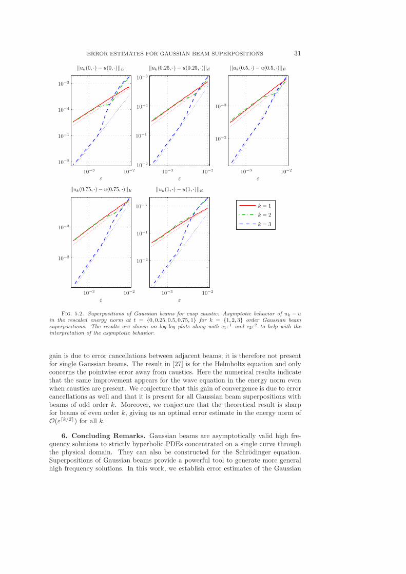
We draw the attention of the reader to the following features in the plots:1. At all t:
(a) The asymptotic behavior of 1-st and 2-nd order solutions is the sameand of order O(ε1).
(b) The asymptotic behavior of 3-rd order solution is of order O(ε2).(c) For large value of ε the error for 2-nd and 3-rd order solutions is dom-
inated by the error induced by the cutoff function. In this region theerror decays exponentially.
(d) For midrange values of ε, 2-nd order solutions experience a fortuitouserror cancellation. This is due to the cutoff function. Changing thecutoff radius η shifts this region.
2. At t = 0.5 and t > 0.5, the asymptotic behavior of the error is unaffected bythe cusp and fold caustics, respectively.
For this example we note that the convergence rate for odd beams k ∈ 1, 3 is infact half an order better than our theoretical estimates. This improvement was alsoobserved and proved for a simplified setting in [27], where the analysis shows that the
ERROR ESTIMATES FOR GAUSSIAN BEAM SUPERPOSITIONS 31
||uk(0, ·) − u(0, ·)||E
ε
||uk(0.25, ·)− u(0.25, ·)||E
ε
||uk(0.5, ·) − u(0.5, ·)||E
ε
||uk(0.75, ·)− u(0.75, ·)||E
ε
||uk(1, ·) − u(1, ·)||E
ε
k = 1
k = 2
k = 3
10−3 10−210−3 10−2
10−3 10−210−3 10−210−3 10−2
10−3
10−2
10−110−3
10−2
10−3
10−2
10−4
10−3
10−2
10−1
10−4
10−3
10−2
10−1
Fig. 5.2. Superpositions of Gaussian beams for cusp caustic: Asymptotic behavior of uk − u
in the rescaled energy norm at t = 0, 0.25, 0.5, 0.75, 1 for k = 1, 2, 3 order Gaussian beam
superpositions. The results are shown on log-log plots along with c1ε1 and c2ε2 to help with the
interpretation of the asymptotic behavior.
gain is due to error cancellations between adjacent beams; it is therefore not presentfor single Gaussian beams. The result in [27] is for the Helmholtz equation and onlyconcerns the pointwise error away from caustics. Here the numerical results indicatethat the same improvement appears for the wave equation in the energy norm evenwhen caustics are present. We conjecture that this gain of convergence is due to errorcancellations as well and that it is present for all Gaussian beam superpositions withbeams of odd order k. Moreover, we conjecture that the theoretical result is sharpfor beams of even order k, giving us an optimal error estimate in the energy norm ofO(ε⌈k/2⌉) for all k.
6. Concluding Remarks. Gaussian beams are asymptotically valid high fre-quency solutions to strictly hyperbolic PDEs concentrated on a single curve throughthe physical domain. They can also be constructed for the Schrodinger equation.Superpositions of Gaussian beams provide a powerful tool to generate more generalhigh frequency solutions. In this work, we establish error estimates of the Gaussian
32 H. LIU, O. RUNBORG AND N. M. TANUSHEV
beam superposition for all strictly hyperbolic PDEs and the Schrodinger equation.Our study gives the surprising conclusion that even if the superposition is done overphysical space, the error is still independent of the number of dimension and of thepresence of caustics. Thus, we improve upon earlier results by Liu and Ralston [22, 23].
Acknowledgement. The authors would like to thank James Ralston and BjornEngquist for many helpful discussions. HL’s research was partially supported bythe National Science Foundation under Kinetic FRG grant No. DMS 07-57227 andgrant No. DMS 09-07963. NMT was partially supported by the National ScienceFoundation under grant No. DMS-0914465 and grant No. DMS-0636586 (UT AustinRTG).
REFERENCES
[1] G. Ariel, B. Engquist, N. M. Tanushev, and R. Tsai. Gaussian beam decomposition of highfrequency wave fields using expectation-maximization. J. Comput. Phys., 230(6):2303–2321, 2011.
[2] V. M. Babic and V. S. Buldyrev. Short-Wavelength Diffraction Theory: Asymptotic Methods,volume 4 of Springer Series on Wave Phenomena. Springer-Verlag, 1991.
[3] V. M. Babic and T. F. Pankratova. On discontinuities of Green’s function of the wave equationwith variable coefficient. Problemy Matem. Fiziki, 6, 1973. Leningrad University, Saint-Petersburg.
[4] V. M. Babic and M. M. Popov. Gaussian summation method (review). Izv. Vyssh. Uchebn.
Zaved. Radiofiz., 32(12):1447–1466, 1989.[5] S. Bougacha, J.L. Akian, and R. Alexandre. Gaussian beams summation for the wave equation
in a convex domain. Commun. Math. Sci., 7(4):973–1008, 2009.[6] V. Cerveny, M. M. Popov, and I. Psencık. Computation of wave fields in inhomogeneous media
— Gaussian beam approach. Geophys. J. R. Astr. Soc., 70:109–128, 1982.[7] B. Engquist and O. Runborg. Computational high frequency wave propagation. Acta Numerica,
12:181–266, 2003.[8] N. R. Hill. Gaussian beam migration. Geophysics, 55(11):1416–1428, 1990.[9] N. R. Hill. Prestack Gaussian beam depth migration. Geophysics, 66(4):1240–1250, 2001.
[10] L. Hormander. Fourier integral operators. I. Acta Math., 127(1-2):79–183, 1971.[11] L. Hormander. On the existence and the regularity of solutions of linear pseudo-differential
equations. L’Enseignement Mathematique, XVII:99–163, 1971.[12] L. Hormander. The analysis of linear partial differential operators. I. Classics in Mathematics.
Springer, Berlin, 2003. Distribution theory and Fourier analysis, Reprint of the 1990edition.
[13] L. Hormander. The analysis of linear partial differential operators. III. Classics in Mathematics.Springer, Berlin, 2007. Pseudo-differential operators, Reprint of the 1994 edition.
[14] S. Jin, H. Wu, and X. Yang. Gaussian beam methods for the Schrodinger equation in the semi-classical regime: Lagrangian and Eulerian formulations. Commun. Math. Sci., 6:995–1020,2008.
[15] A. P. Katchalov and M. M. Popov. Application of the method of summation of Gaussian beamsfor calculation of high-frequency wave fields. Sov. Phys. Dokl., 26:604–606, 1981.
[16] J. B. Keller. Corrected Bohr-Sommerfeld quantum conditions for nonseparable systems. Ann.
Physics, 4:180–188, 1958.[17] L. Klimes. Expansion of a high-frequency time-harmonic wavefield given on an initial surface
into Gaussian beams. Geophys. J. R. astr. Soc., 79:105–118, 1984.[18] L. Klimes. Discretization error for the superposition of Gaussian beams. Geophys. J. R. Astr.
Soc., 86:531–551, 1986.[19] Yu. A. Kravtsov. On a modification of the geometrical optics method. Izv. VUZ Radiofiz.,
7(4):664–673, 1964.[20] S. Leung and J. Qian. Eulerian Gaussian beams for Schrodinger equations in the semi-classical
regime. J. Comput. Phys., 228:2951–2977, 2009.[21] S. Leung, J. Qian, and R. Burridge. Eulerian Gaussian beams for high frequency wave propa-
gation. Geophysics, 72:SM61–SM76, 2007.[22] H. Liu and J. Ralston. Recovery of high frequency wave fields for the acoustic wave equation.
Multiscale Model. Sim., 8(2):428–444, 2009.
ERROR ESTIMATES FOR GAUSSIAN BEAM SUPERPOSITIONS 33
[23] H. Liu and J. Ralston. Recovery of high frequency wave fields from phase space–based mea-surements. Multiscale Model. Sim., 8(2):622–644, 2010.
[24] D. Ludwig. Uniform asymptotic expansions at a caustic. Comm. Pure Appl. Math., 19:215–250,1966.
[25] V. P. Maslov and M. V. Fedoriuk. Semiclassical approximation in quantum mechanics, volume 7of Mathematical Physics and Applied Mathematics. D. Reidel Publishing Co., Dordrecht,1981. Translated from the Russian by J. Niederle and J. Tolar, Contemporary Mathematics,5.
[26] M. Motamed and O. Runborg. A wave front Gaussian beam method for high-frequency wavepropagation. In Proceedings of WAVES 2007, University of Reading, UK, 2007.
[27] M. Motamed and O. Runborg. Taylor expansion and discretization errors in Gaussian beamsuperposition. Wave Motion, 2010.
[28] M. M. Popov. A new method of computation of wave fields using Gaussian beams. Wave
Motion, 4:85–97, 1982.[29] J. Qian and L. Ying. Fast Gaussian wavepacket transforms and Gaussian beams for the
Schrodinger equation. J. Comput. Phys., 229:7848–7873, 2010.[30] J. Ralston. Gaussian beams and the propagation of singularities. In Studies in partial differ-
ential equations, volume 23 of MAA Stud. Math., pages 206–248. Math. Assoc. America,Washington, DC, 1982.
[31] V. Rousse and T. Swart. Global L2-boundedness theorems for semiclassical Fourier integraloperators with complex phase. arxiv:0710.4200v3, 2007.
[32] V. Rousse and T. Swart. A mathematical justification for the Herman–Kluk propagator. Comm.
Math. Phys., 286(2):725–750, 2009.[33] O. Runborg. Mathematical models and numerical methods for high frequency waves. Commun.
Comput. Phys., 2:827–880, 2007.[34] N. M. Tanushev. Superpositions and higher order Gaussian beams. Commun. Math. Sci.,
6(2):449–475, 2008.[35] N. M. Tanushev, B. Engquist, and R. Tsai. Gaussian beam decomposition of high frequency
wave fields. J. Comput. Phys., 228(23):8856–8871, 2009.[36] N. M. Tanushev, J. Qian, and J. V. Ralston. Mountain waves and Gaussian beams. Multiscale