36
Chapter 1: Introduction – A Simple Mathematical Model – Conservation Laws – MATLAB Fundamentals – Computer Programming – Programming with Matlab
| Date post: | 12-Jul-2015 |
| Category: |
Technology |
| Upload: | batuhan-yildirim |
| View: | 111 times |
| Download: | 0 times |
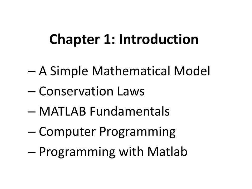
Chapter 1: Introduction
– A Simple Mathematical Model
– Conservation Laws
– MATLAB Fundamentals
– Computer Programming
– Programming with Matlab

A simple Mathematical Model
mgFg
2vcF dD
Problem of a falling object in air:
Fg= Force of gravity
FD=Drag force
m=mass
v(t)= Velocity of the object
cd= Drag coefficient
(Equation of motion)dt
dvmmaFFF Dgnet
m
dt
dvmvcmg d
2 )(tvv
2vm
cg
dt
dv d An Ordinary Differential Equation (ODE)
Need to solve for v(t)
Newton’s 2nd law:
Initial condition: The object is initially at rest
2vm
cg
dt
dv d
0;0 vt
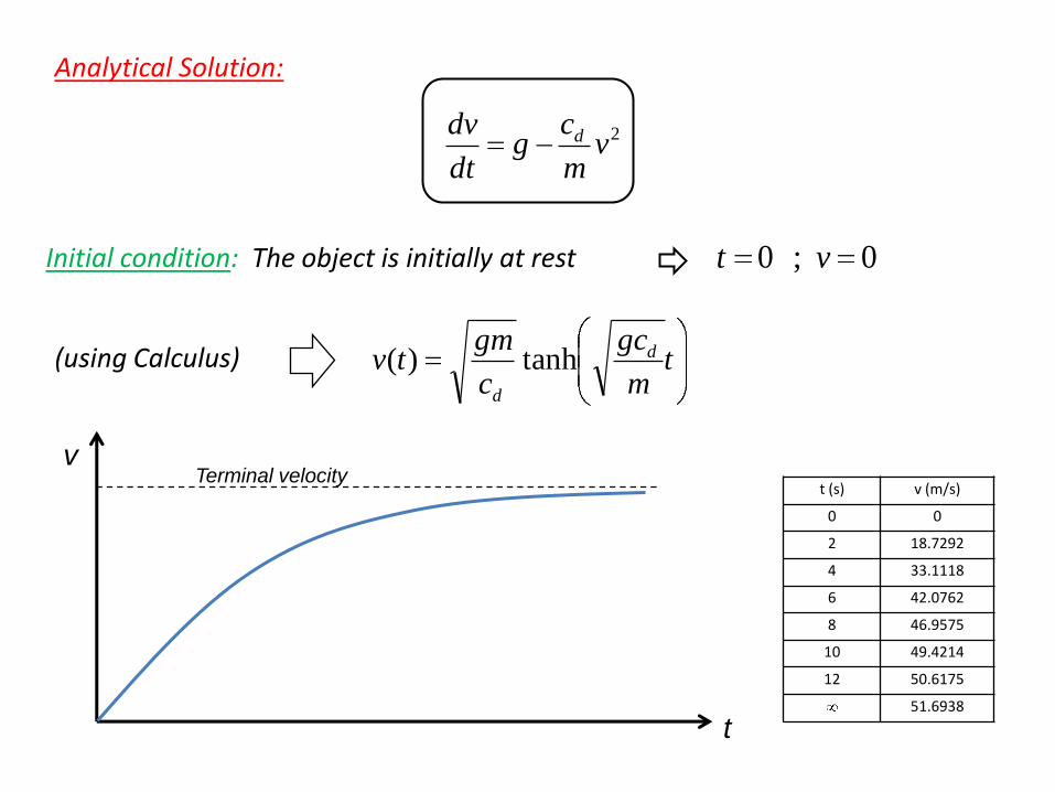
Analytical Solution:
tm
gc
c
gmtv d
d
tanh)(
v
t
Terminal velocityt (s) v (m/s)
0 0
2 18.7292
4 33.1118
6 42.0762
8 46.9575
10 49.4214
12 50.6175
51.6938
(using Calculus)
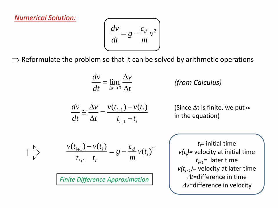
Numerical Solution:
2vm
cg
dt
dv d
ii
ii
tt
tvtv
t
v
dt
dv
1
1 )()(
Reformulate the problem so that it can be solved by arithmetic operations
ti= initial timev(ti)= velocity at initial time
ti+1= later timev(ti+1)= velocity at later time
t=difference in timev=difference in velocity
(Since t is finite, we put in the equation)
2
1
1 )()()(
id
ii
ii tvm
cg
tt
tvtv
t
v
dt
dv
t 0lim (from Calculus)
Finite Difference Approximation
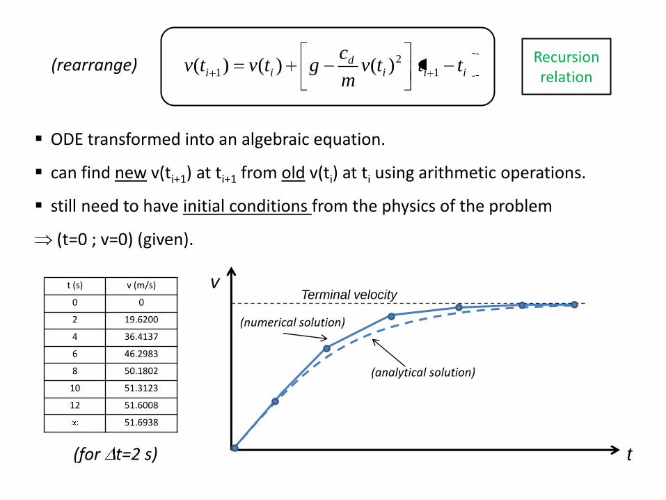
(rearrange)iii
dii tttv
m
cgtvtv 1
2
1 )()()(
ODE transformed into an algebraic equation.
can find new v(ti+1) at ti+1 from old v(ti) at ti using arithmetic operations.
still need to have initial conditions from the physics of the problem
(t=0 ; v=0) (given).
Recursion relation
t (s) v (m/s)
0 0
2 19.6200
4 36.4137
6 46.2983
8 50.1802
10 51.3123
12 51.6008
51.6938
(for t=2 s)
v
t
Terminal velocity
(analytical solution)
(numerical solution)
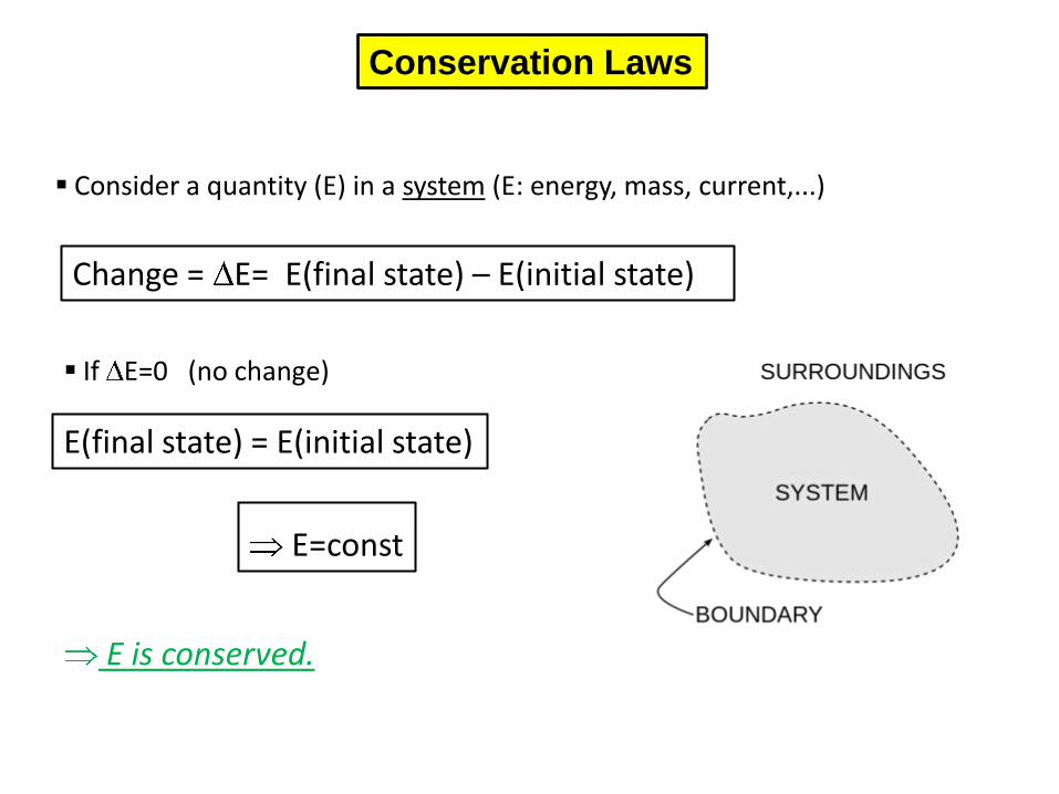
Conservation Laws
Consider a quantity (E) in a system (E: energy, mass, current,...)
Change = E= E(final state) – E(initial state)
If E=0 (no change)
E(final state) = E(initial state)
E=const
E is conserved.
Conservation Laws in Engineering:
Conservation of Energy (All)
Conservation of Mass (Chemical, Mechanical, etc.)
Conservation of Momentum (Civil; Mechanical, etc.)
Conservation of Charge (Electrical, etc.)
...
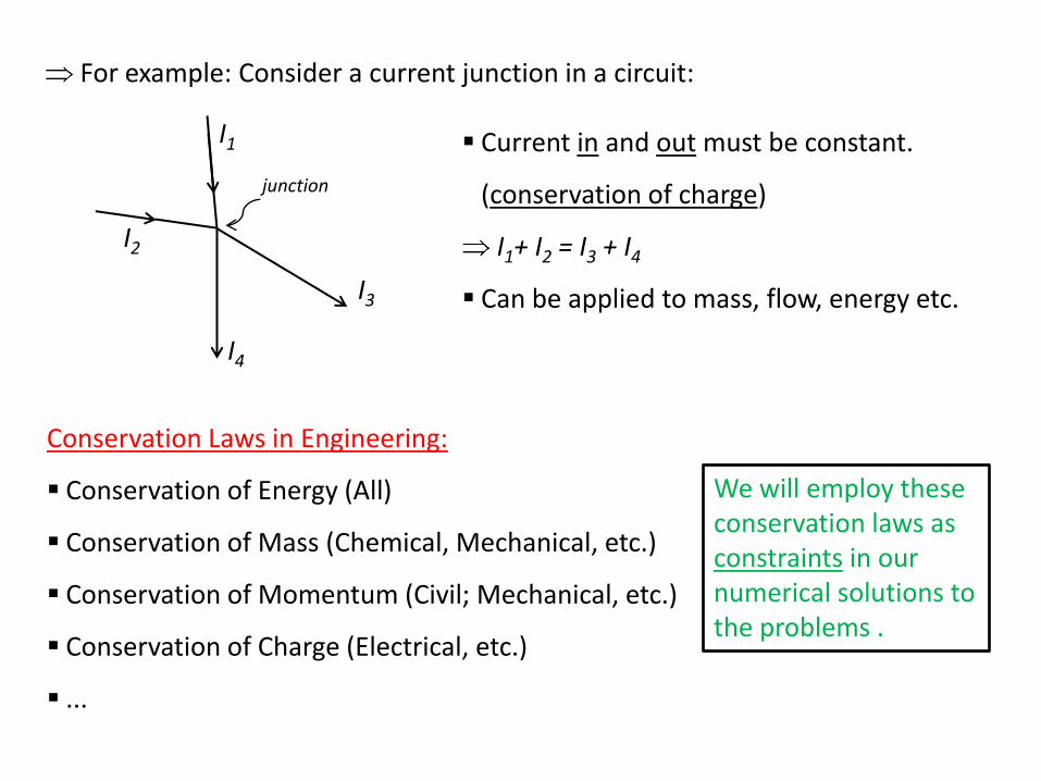
For example: Consider a current junction in a circuit:
I1
I2
I3
I4
Current in and out must be constant.
(conservation of charge)
I1+ I2 = I3 + I4
Can be applied to mass, flow, energy etc.
We will employ these conservation laws as constraints in our numerical solutions to the problems .
junction

Matlab Fundamentals
Command window: to enter commands and data.
Graphics window: to plot graphics.
Edit window: create and edit M-files.
Command window:
Can be operated just like a calculator
>> 55-16
ans=
39
Define a scalar value
>> a=4
a=
4
Assignments can be suppressed by semicolon (;)
>> a=4;
(just stored in memory w/o displaying)
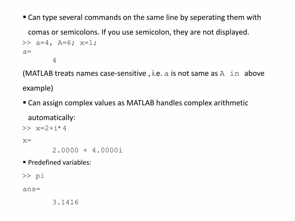
Can type several commands on the same line by seperating them with
comas or semicolons. If you use semicolon, they are not displayed.>> a=4, A=6; x=1;
a=
4
(MATLAB treats names case-sensitive , i.e. a is not same as A in above
example)
Can assign complex values as MATLAB handles complex arithmetic
automatically:>> x=2+i*4
x=
2.0000 + 4.0000i
Predefined variables:
>> pi
ans=
3.1416
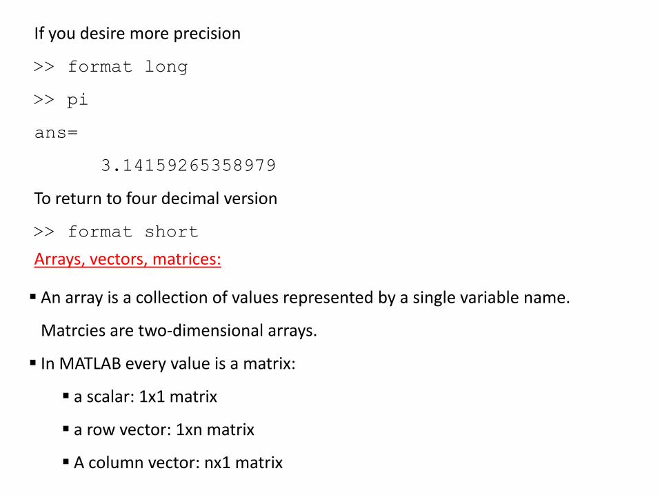
If you desire more precision
>> format long
>> pi
ans=
3.14159265358979
To return to four decimal version
>> format short
An array is a collection of values represented by a single variable name.
Matrcies are two-dimensional arrays.
In MATLAB every value is a matrix:
a scalar: 1x1 matrix
a row vector: 1xn matrix
A column vector: nx1 matrix
Arrays, vectors, matrices:
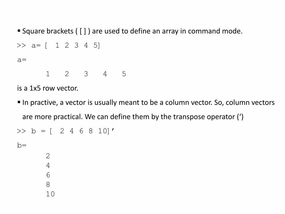
Square brackets ( [ ] ) are used to define an array in command mode.
>> a= [ 1 2 3 4 5]
a=
1 2 3 4 5
is a 1x5 row vector.
In practive, a vector is usually meant to be a column vector. So, column vectors
are more practical. We can define them by the transpose operator (‘)
>> b = [ 2 4 6 8 10]’
b=
2
4
6
8
10

A matrix of values can be assigned as follows:
>> A = [1 2 3 ; 4 5 6; 7 8 9]
A=
1 2 3
4 5 6
7 8 9
Alternatively “Enter” key can be used at the end of each row to define A:
>> A =[ 1 2 3
4 5 6
7 8 9 ];
(strike Enter key after 3 and 6)
To see the list of all variables at any session:
>> who
Your variables are:
A a ans b x
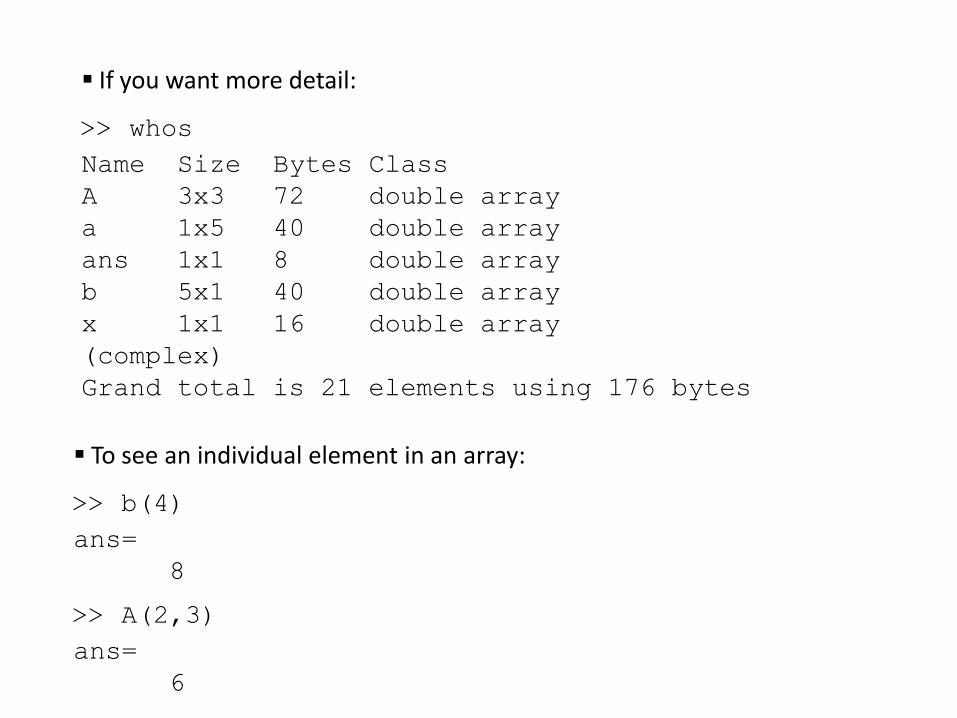
If you want more detail:
>> whos
Name Size Bytes Class
A 3x3 72 double array
a 1x5 40 double array
ans 1x1 8 double array
b 5x1 40 double array
x 1x1 16 double array
(complex)
Grand total is 21 elements using 176 bytes
To see an individual element in an array:
>> b(4)
ans=
8
>> A(2,3)
ans=
6

Some predefined matrices are very useful.
>> E= zeros(2,3)
E=
0 0 0
0 0 0
>> u=ones(1,3)
u=
1 1 1
Colon (:) operator is very useful to generating arrays:
>> t=1:5
t=
1 2 3 4 5
If you want increment other than 1, then you type:
>> t= 1:0.5:3
t=
1.0000 1.5000 2.000 2.500 3.0000
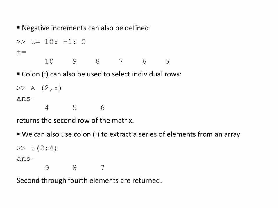
Negative increments can also be defined:
>> t= 10: -1: 5
t=
10 9 8 7 6 5
Colon (:) can also be used to select individual rows:
>> A (2,:)
ans=
4 5 6
returns the second row of the matrix.
We can also use colon (:) to extract a series of elements from an array
>> t(2:4)
ans=
9 8 7
Second through fourth elements are returned.
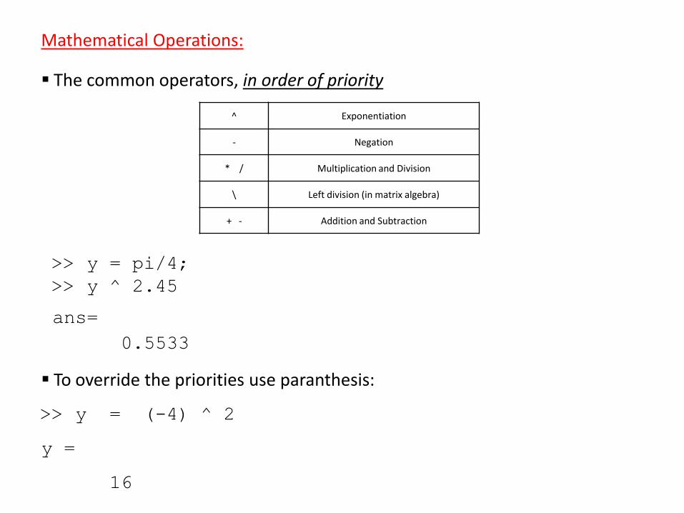
Mathematical Operations:
The common operators, in order of priority
^ Exponentiation
- Negation
* / Multiplication and Division
\ Left division (in matrix algebra)
+ - Addition and Subtraction
>> y = pi/4;
>> y ^ 2.45
ans=
0.5533
To override the priorities use paranthesis:
>> y = (-4) ^ 2
y =
16
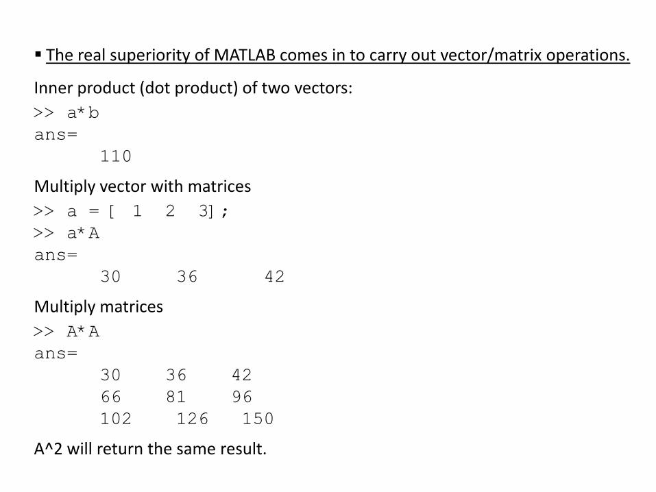
The real superiority of MATLAB comes in to carry out vector/matrix operations.
Inner product (dot product) of two vectors:
>> a*b
ans=
110
Multiply vector with matrices
>> a = [ 1 2 3];
>> a*A
ans=
30 36 42
Multiply matrices
>> A*A
ans=
30 36 42
66 81 96
102 126 150
A^2 will return the same result.
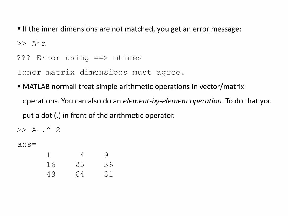
If the inner dimensions are not matched, you get an error message:
>> A*a
??? Error using ==> mtimes
Inner matrix dimensions must agree.
MATLAB normall treat simple arithmetic operations in vector/matrix
operations. You can also do an element-by-element operation. To do that you
put a dot (.) in front of the arithmetic operator.
>> A .^ 2
ans=
1 4 9
16 25 36
49 64 81
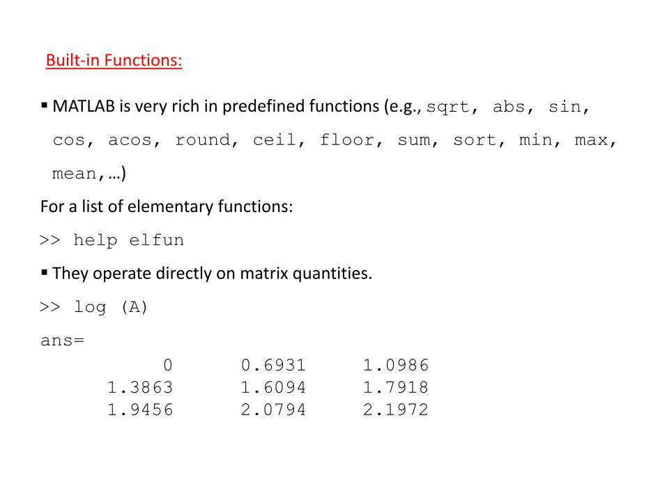
Built-in Functions:
MATLAB is very rich in predefined functions (e.g., sqrt, abs, sin,
cos, acos, round, ceil, floor, sum, sort, min, max,
mean,…)
For a list of elementary functions:
>> help elfun
They operate directly on matrix quantities.
>> log (A)
ans=
0 0.6931 1.0986
1.3863 1.6094 1.7918
1.9456 2.0794 2.1972
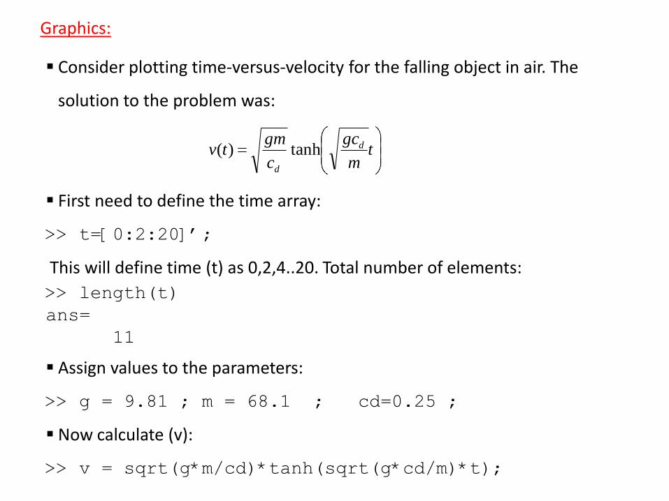
Graphics:
Consider plotting time-versus-velocity for the falling object in air. The
solution to the problem was:
First need to define the time array:
>> t=[0:2:20]’;
This will define time (t) as 0,2,4..20. Total number of elements:
>> length(t)
ans=
11
Assign values to the parameters:
>> g = 9.81 ; m = 68.1 ; cd=0.25 ;
Now calculate (v):
>> v = sqrt(g*m/cd)*tanh(sqrt(g*cd/m)*t);
tm
gc
c
gmtv d
d
tanh)(
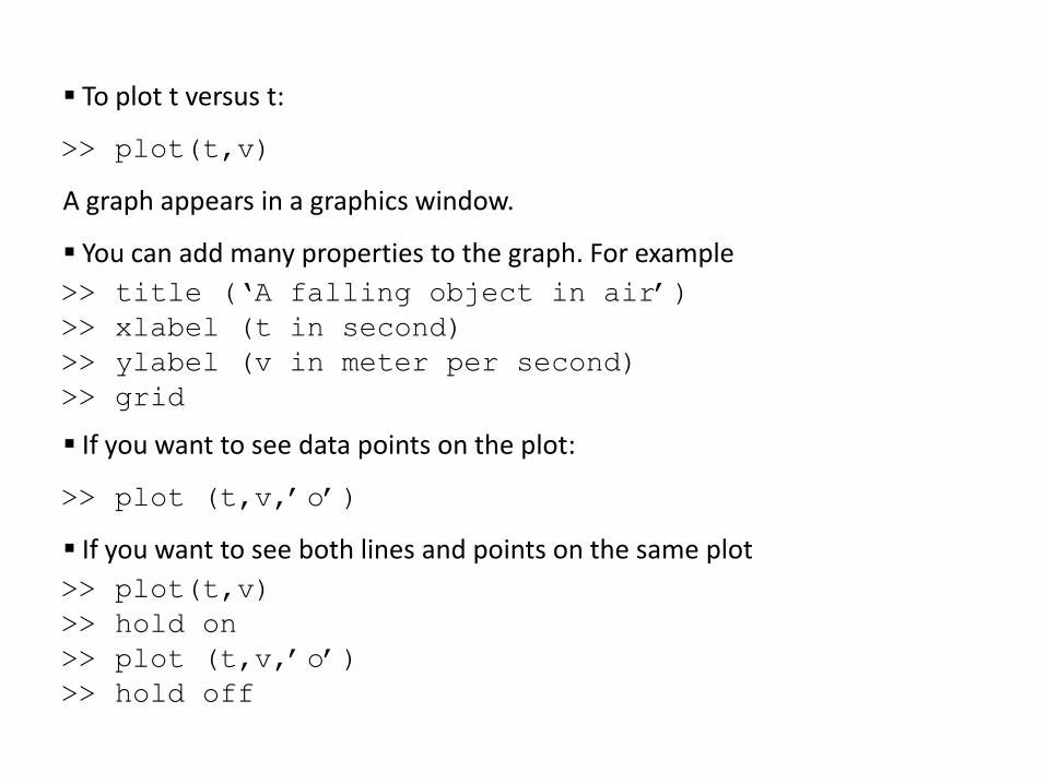
To plot t versus t:
>> plot(t,v)
A graph appears in a graphics window.
You can add many properties to the graph. For example
>> title (‘A falling object in air’)
>> xlabel (t in second)
>> ylabel (v in meter per second)
>> grid
If you want to see data points on the plot:
>> plot (t,v,’o’)
If you want to see both lines and points on the same plot
>> plot(t,v)
>> hold on
>> plot (t,v,’o’)
>> hold off

Step 1: Start the calculation
Step 2: Input a value for A
Step 3: Input a value for B
Step 4: Add A to B and call the
answer C
Step 5: Output the value for C
Step 6: End the calculation
Start
Input A
A simple addition algorithm
using natural language
The same algorithm using a flowchart
end
Input B
Add A and BCall the result C
Output C

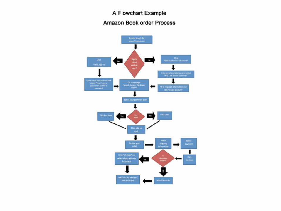
A flowchart is a type of diagram that represents an algorithm.
Steps are shown by boxes of various kinds.
The order of the flow is shown by arrows.
Flowcharts:
Monopoly flowchart
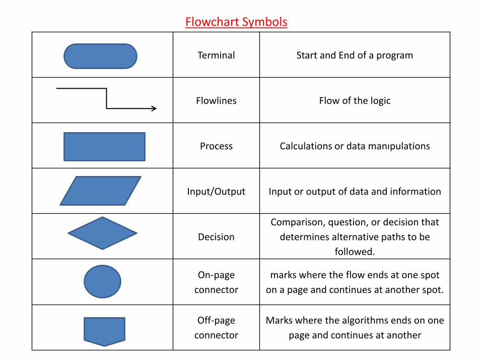
Terminal Start and End of a program
Flowlines Flow of the logic
Process Calculations or data manıpulations
Input/Output Input or output of data and information
Decision
Comparison, question, or decision that
determines alternative paths to be
followed.
On-page
connector
marks where the flow ends at one spot
on a page and continues at another spot.
Off-page
connector
Marks where the algorithms ends on one
page and continues at another
Flowchart Symbols
An algorithm is the step-by-step procedure for calculations.
It is a finite list of well-defined instruction for calculting a function.
Can be expressed in many ways: natural languages, pseudocodes,
flowcharts, etc.
Natural languages are usually ambigous and not a preferred way and
rarely used for comlex algorithms.
Programming lanuguages express algorithms so that they can be
executed by a computer.
Algorithms:
It is the comprehensive process of
(problem algorithm coding executables)
Computer Programming
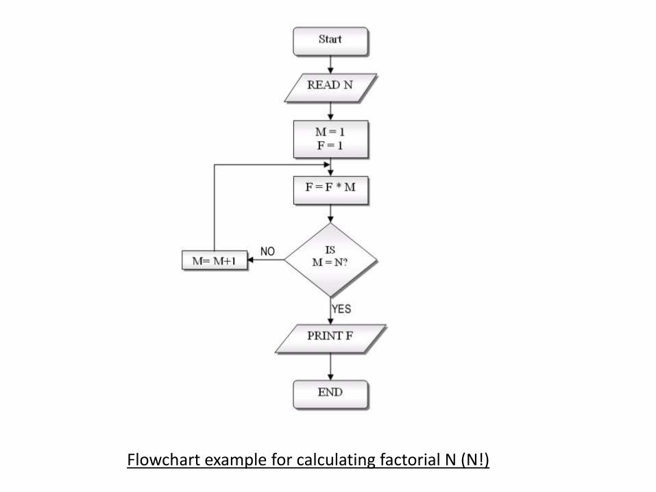
Flowchart example for calculating factorial N (N!)

Pseudocode is a higher-level method for describing an algorithm.
It uses the structural convention of a programming language but is
intended for human reading rather than machine reading.
It is easier for people to understand than a programming code.
It is environment-independent description of the key principles of an
algorithm.
It omits the details not essential for human understanding of the algorithm
(such as variable declarations).
It can also advantage of natural language.
It is commonly used in textbooks and scientific publications.
No standard for pseudocode syntax exists.
Pseudocodes:
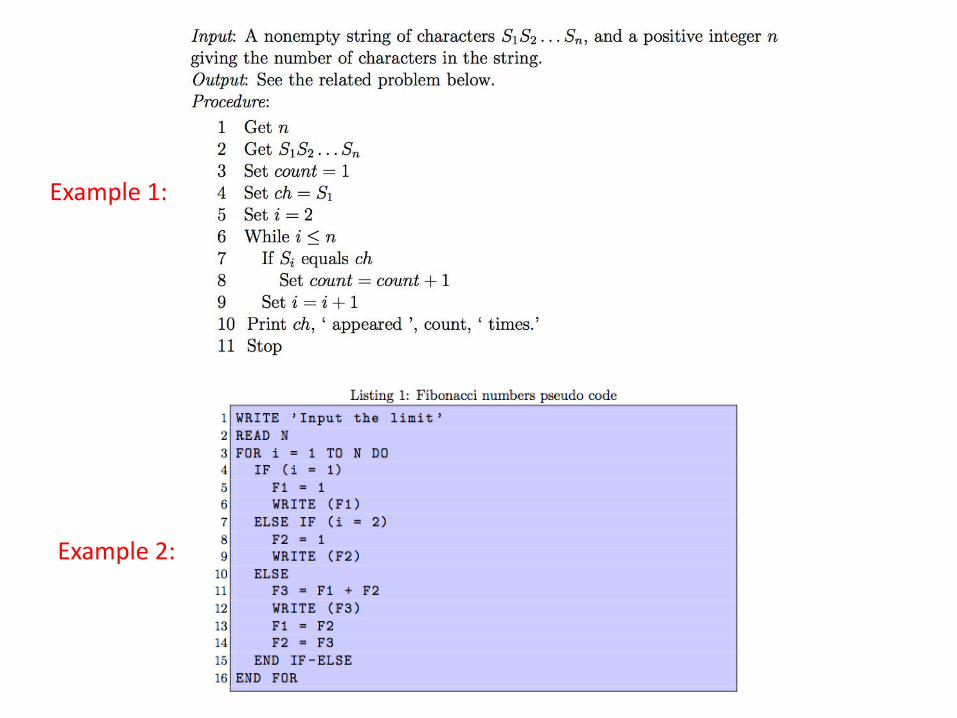
Example 1:
Example 2:

FlowchartPseudocode
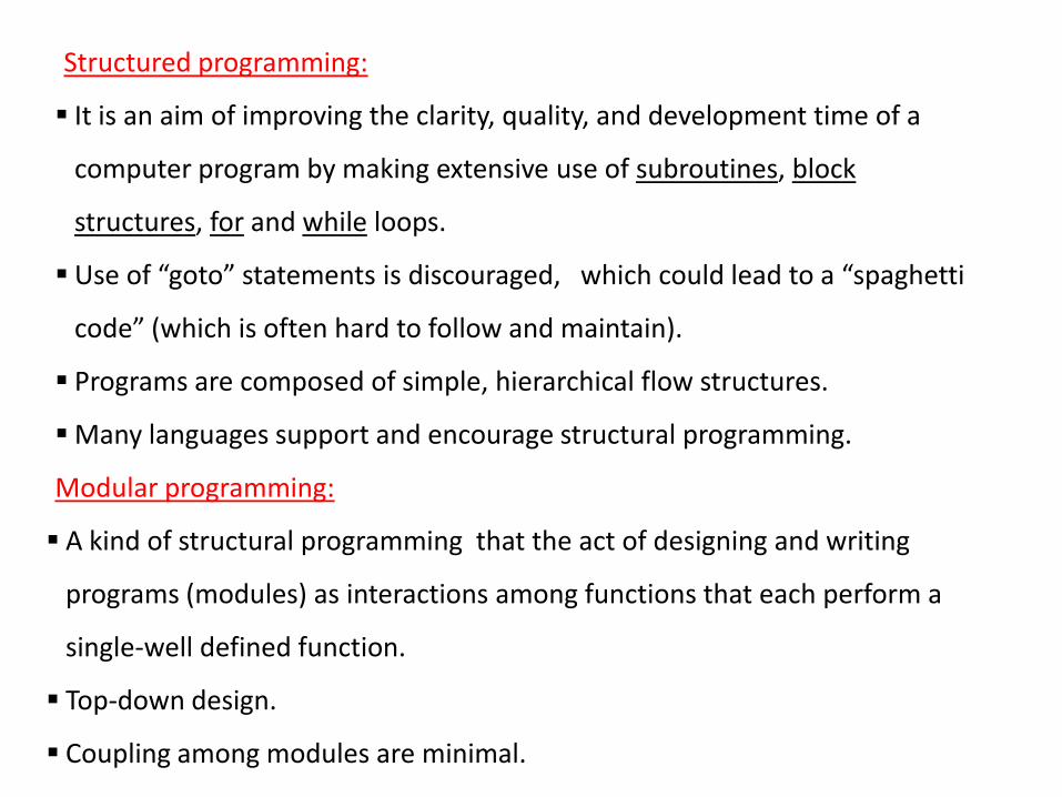
Structured programming:
It is an aim of improving the clarity, quality, and development time of a
computer program by making extensive use of subroutines, block
structures, for and while loops.
Use of “goto” statements is discouraged, which could lead to a “spaghetti
code” (which is often hard to follow and maintain).
Programs are composed of simple, hierarchical flow structures.
Many languages support and encourage structural programming.
Modular programming:
A kind of structural programming that the act of designing and writing
programs (modules) as interactions among functions that each perform a
single-well defined function.
Top-down design.
Coupling among modules are minimal.
Programming with Matlab
We use the editor window to generate M-files.
M-files contain a series of statements that can be run all at once.
Files are stored with extension .m
M-files can be script files or function files.
M-files:
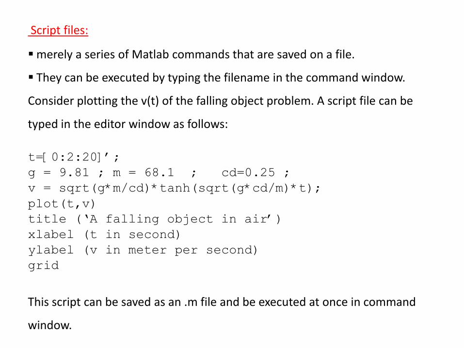
Script files:
merely a series of Matlab commands that are saved on a file.
They can be executed by typing the filename in the command window.
Consider plotting the v(t) of the falling object problem. A script file can be
typed in the editor window as follows:
t=[0:2:20]’;
g = 9.81 ; m = 68.1 ; cd=0.25 ;
v = sqrt(g*m/cd)*tanh(sqrt(g*cd/m)*t);
plot(t,v)
title (‘A falling object in air’)
xlabel (t in second)
ylabel (v in meter per second)
grid
This script can be saved as an .m file and be executed at once in command
window.

Function files:
M-files that start with the word function.
Unlike script files they can accept input arguments and return outputs.
They must be stored as “functionname.m”.
Consider writing a function freefall.m for the falling body problem:
function v = freefall(t,m,cd)
% Inputs
% t(nx1) = time (nx1) in second
% m = mass of the object (kg)
% cd = drag coefficient (kg/m)
% Output
% v(nx1) = downward velocity (m/s)
g = 9.81 ; % acceleration of gravity
v = sqrt(g*m/cd)*tanh(sqrt(g*cd/m)*t);
return
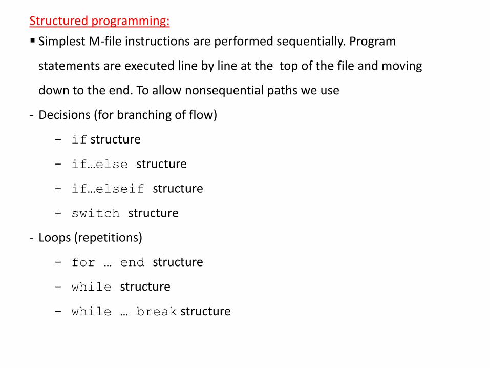
Simplest M-file instructions are performed sequentially. Program
statements are executed line by line at the top of the file and moving
down to the end. To allow nonsequential paths we use
- Decisions (for branching of flow)
- if structure
- if…else structure
- if…elseif structure
- switch structure
- Loops (repetitions)
- for … end structure
- while structure
- while … break structure
Structured programming:
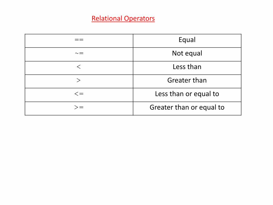
Relational Operators
== Equal
~= Not equal
< Less than
> Greater than
<= Less than or equal to
>= Greater than or equal to


