Estimating Gravity Equation Models in the Presence of Sample Selection and Heteroskedasticity Bo Xiong 1 Sixia Chen 2 1 University of California, Davis [email protected]2 Iowa State University [email protected]Selected Paper prepared for presentation at the Agricultural & Applied Economics Association’s 2012 AAEA Annual Meeting, Seattle, Washington, August 12-14, 2012 Copright 2012 by Bo Xiong and Sixia Chen. All rights reserved. Readers may make verbatim copies of this document for non-commercial purposes by any means, provided that this copyright notice appears on all such copies.
Transcript
Estimating Gravity Equation Models in the Presence of Sample Selection and
Method of Moments, intensive margin, extensive margin, market access
JEL classification: F10, C10
Bo Xiong (correspondence author), [email protected] , is a postdoctoral researcher in the Agricultural and Resource Economics Department, University of California, Davis; and Sixia Chen, [email protected], is a senior survey methodologist at the Westat corporation, Rockville, Maryland. We thank John Beghin and Joseph Herriges at Iowa State University, and participants in the session of non-tariff barriers at the 2012 Agricultural and Applied Economics Association annual meeting for helpful discussions. The usual disclaimer applies.
1
1. Introduction
The gravity equation model has been a long-time workhorse in international trade since
Tinbergen (1962). It posits that the bilateral trade flow from one country to another can
be explained by the two countries’ income levels, geographic distance, and various other
factors (such as import tariffs, non-tariff regulations, contiguity condition, historical
colonial relationship, and religion similarity between the trading partners) that could
affect the cost of trade. In addition to its empirical success in fitting trade data reasonably
well (Baldwin and Taglioni, 2006), the gravity equation model has recently received
more recognition because of the development of its microeconomic foundations.1
Following Anderson (1979), Anderson and van Wincoop (2003) derive a full
specification of the gravity equation model with trade costs from the utility maximization
behavior of a representative consumer with Constant Elasticity of Substitution (CES)
preferences. Most importantly, they emphasize the role of countries’ multi-lateral trade
resistance terms in a cross-sectional gravity equation analysis. Novy (2010) innovates a
gravity equation under a general equilibrium framework with a translog demand system.
Markusen (1986) and Bergstrand (1985, 1989) introduce non-homothetic preferences in
gravity equation models and shed light on the impacts of per-capital income on trade
patterns. Deardorff (1998) shows that a gravity equation can emerge from a Heckscher-
Ohlin setting as well. Evenett and Keller (2002) report that both the Heckscher-Ohlin
theory and the monopolistic-competition trade theory can lead to the gravity equation and
that each provides unique insights to the international variation of production and trade
patterns. In a comprehensive review, Feenstra, Markusen, and Rose (2001) examine how
1 Interested readers are referred to Anderson (2010) for a survey on the theoretical and empirical
developments of the gravity equation approach to trade.
2
various trade theories are linked to the gravity equation approach and provide evidence in
favor of the monopolistic-competition theory and the reciprocal-dumping theory.
Following the new trade theory of heterogeneous firms, Helpman, Melitz, and Rubinstein
(2008) (HMR hereafter) build up a generalized gravity equation with firms facing fixed
costs of exporting. Their model predicts that only the most productive firms are able to
overcome the fixed cost of trade and penetrate foreign markets, and that trade
liberalization induces more firms to participate in the world market.
Despite the rapid development of the microeconomic functions for the gravity
equation model, there is no consensus in the literature on how to statistically estimate a
gravity equation in the presence of the two stylized features of trade data: sample
selection and heteroskedasticity. On the one hand, zeros are commonly found in trade
data, which could give rise to the classical sample selection issue. For example, zeros can
take up nearly 50% of all bilateral trade records at the national level (e.g., HMR). Even
with panel data covering more recent years in agricultural sectors, zeros easily account
for 30% of all the observations (Sun and Reed, 2010; Grant and Boys, 2012). The
treatment of these frequent zeros is an important concern in the analysis of trade policies
for at least two reasons. First, from a statistical viewpoint, the omission or mis-treatment
of zeros could lead to the sample selection bias, as defined by Heckman (1979), unless
the zeros correspond to “missing at random.”2 Second, from an economic perspective, the
modeling of zeros directly speaks to the question whether trade polices improve or
deteriorate market access for sporadic traders who frequently opt out of the world market.
Such market access effect is of particular importance when the policies of interest play a
2 Interested readers are referred to Little and Rubin (1987) for a classification of missing data problems.
3
major role in determining the cost of trade for smallholder exporters from the developing
world. For instance, Shepherd (2010) shows that the reduction in export costs, tariffs, and
transport costs can encourage developing countries to export to more destinations.
Besedes and Prusa (2011) argue that developing countries are more likely to experience
long-run export growth if new entrants to world market have a better chance to survive
beyond the first year. Bergin and Lin (2008) demonstrate that currency unions facilitate
international trade predominantly through increasing the number of exporting firms and
the number of traded products.
On the other hand, trade data often exhibit heteroskedasticity. The data sample of
a gravity equation analysis usually consists of bilateral trade flows collected from
multiple countries, which naturally gives ground to heteroskedasticity. In general,
heteroskedasticity is less a concern as long as the model is correctly specified because it
does not undermine the consistency of estimates. In a gravity equation analysis, however,
heteroskedasticity challenges the common practice of logarithmic transformation. As
Santos Silva and Tenreyro (2006) (SST hereafter) show, if the true gravity equation
model is in its multiplicative form and heteroskedasticity is present, estimates from the
log-linearized gravity equation models can be severely biased. Arguably, the above two
features of trade data, sample selection and heteroskedasticity, warn against the use of the
Ordinary Least Square technique. As various new estimators for the gravity equation
model are being proposed, two camps emerge in the literature.
One camp in the debate focuses on the economics of zero trade flows. The new
trade theory, pioneered by Melitz (2003) and later developed by several others such as
Chaney (2008) and HMR, posits that the absence of trade can be attributed to firms’ self-
4
selection behavior: zero trade flow is observed when none of the firms in the potential
exporting country is productive enough to overcome the fixed costs imposed by the
destination market. Therefore, zeros can be seen as generated from a selection process,
which gives grounds to the Heckman sample selection model (Heckman, 1979), or, to a
less degree, the E.T.-Tobit model (Eaton and Tamura, 1994). In a Heckman sample
selection model, the selection equation fully captures zeros and explains why trade takes
place at all, while the outcome equation characterizes the volume of the trade conditional
on trade occurring. The E.T.-Tobit model treats zeros as censored outcomes and assumes
that there is minimal threshold to jump if trade flows are to be observed. Besides well
connected with the new trade theory, both the Heckman sample selection model and the
E.T.-Tobit model deliver rich comparative statics. Specifically, one can decompose the
effect of trade liberalization into the intensive margin (the intensification of pre-existing
trade) and the extensive margin (the creation of new trade partnership).3 Nevertheless,
built upon the log-linearized version of the gravity equation, the Heckman sample
selection model or the E.T.-Tobit model may deliver biased estimates when trade data
exhibits heteroskedasticity in levels.
The other camp in the debate suggests specifying the gravity equation in its
multiplicative form and estimating it via some variants of count data models. In
particular, SST propose the Poisson Pseudo Maximum Likelihood (PPML) estimator to
accommodate heteroskedasticity in trade data. By estimating trade flows in levels, as
opposed to in logs, the PPML estimator permits zeros and has been shown to be robust to
3 Throughout the paper, we refer to the extensive margin of trade as new trade partnership at national level. Alternatively, the extensive margin can refer to the newly entered firms (HMR), or the newly traded varieties (Hummels and Klenow, 2005), or the newly reached consumers (Arkolakis, 2010). We omit these dimensions because our data is at national level.
5
a wide range of heteroskedastic patterns. However, Martin and Pham (2008) note that the
PPML estimates are severely biased when zeros are not random outcomes.4 Some
variants of the PPML estimator are also proposed. For example, Burger, Linders, and
Oort (2009) consider the Negative Binomial Pseudo Maximum Likelihood estimator
(NBPML), the Zero Inflated Poisson Pseudo Maximum Likelihood estimator (ZIPPML),
and the Zero Inflated Negative Binomial Pseudo Maximum Likelihood estimator
(ZINBPML). Although with merits of their own (such as permitting over-dispersion and
excessive zeros), none of the above variants is robust to a change of the unit of
measurement of the dependent variable (e.g., different estimates result when trade flows
are measured in thousands of dollars instead of dollars). Such a defect arguably prevents
NBPML, ZIPPML, and ZINBPML from being widely adopted.
We contribute to the estimation of gravity equation models in two important
ways. First, we propose a Two-Step Method of Moments (TS-MM) estimator that
simultaneously deals with sample selection and heteroskedasticity. The estimator works
as follows. In the first step, we characterize the binary decision of trade or no trade by a
selection process and predict the probability of trade accordingly. As a result, we can
explain the absence of trade and evaluate determinants of market access. In the second
step, we capture positive trade flows by a gravity equation in its multiplicative form, with
the potential sample selection bias corrected. By estimating the gravity equation via the
method of moments approach and constructing the heteroskedasticity-resistant standard
errors (White, 1980), we are able to obtain consistent point estimates and conduct
statistical inferences correspondingly. Our Monte-Carlo experiments confirm that the
4 In a reply, Silva and Tenreyro (2011) show that the PPML estimator is able to accommodate high
frequency of zeros, without fully addressing the sample selection issue.
6
proposed TS-MM estimator strictly dominates the Heckman, PPML, and E.T.-Tobit
models under certain qualifications.
Second, we suggest a model selection strategy that allows one to choose the most
appropriate estimator in practice. Our proposed strategy utilizes both economic theory
and statistical tests. Guided by the new trade theory, we argue that, in the presence of
sample selection and heteroskedasticity, the Heckman sample selection model, the TS-
MM model, and the PPML model are three competing estimators to choose from. We
employ the MacKinnon-White-Davidson test (MacKinnon, White, and Davidson, 1983)
to differentiate the Heckman sample selection model and the TS-MM model. The
survivor of the MWD test is considered the most preferred estimator if evidence of
sample selection bias is found. Otherwise, we use the Theil’s inequality coefficient
(Theil, 1961), as a measure of goodness of fit, to further compare the estimator surviving
the MWD test with the PPML estimator. We illustrate how the proposed estimator and
model selection work by re-examining the bilateral world trade in 1990.
The rest of the article is organized as follows. Section 2 introduces the TS-MM
estimator and discusses its properties. Section 3 uses a set of Monte-Carlo experiments to
assess the performance of various estimators. Section 4 presents the model selection
strategy. Section 5 applies the TS-MM estimator and the model selection strategy to the
data set in SST. Section 6 concludes.
2. The Gravity Equation and the Two-Step Method of Moments Estimator
The gravity equation approach to trade posits that country j ’s import from country i ,
ijM , can be characterized by
7
(1) exp( )ij i j ij ijM Y Y D X ,
where iY and jY denote country i and j ’s characteristics (e.g., GDP, population,
remoteness to the rest of the world); ijD includes any trade cost terms that are specific to
the country pair (e.g., applied tariff rates, geographic distance, contiguity condition,
historical colonial relationship, religion similarity, and the existence of preferential trade
agreements);5 , , and are parameters to be estimated. Simple algebra leads to the last
term in equation (1), where ijX is a row vector containing all explanatory variables in
their log scales and is a column vector stacking all parameters. To take the gravity
equation to practice, one needs to specify the stochastic version of (1), which we pursue
next.
Motivated by the new trade theory, we explicitly account for the absence of trade
by introducing a selection process. Specifically, we set up the stochastic gravity equation
model as follows:
(2a) * exp( )ij ij ijM X ,
(2b) *ij ij ijd Z ,
(2c) )0( * ijij dId ,
(2d) *ij ij ijM d M .
5 Interested readers are referred to Anderson and van Wincoop (2004) for a detailed discussion of trade
costs.
8
*ijM is the notional trade flow from country i to country j in the absence of fixed cost of
trade.6 *ijd is the latent variable for the binary trade decision ijd which equals one if
country j imports from country i , and 0 otherwise. ijZ contains all factors that potentially
affect the fixed cost of trade between the two countries, and is the associated vector of
parameters. ijM is the observed trade flow, which is a product of the binary decision and
the notional trade flow. As in Heckman (1979), we assume that ij and ij are two
idiosyncratic terms following a bivariate normal distribution.7 Specifically,
11 12
21 22
0,
0ij ij
ij
uN
, where 12 21 . The correlation between the two
idiosyncratic terms accounts for omitted variables that affect both the fixed and variable
costs of trade. Noticeably, heteroskedasticity is allowed because ij11 varies across
countries.
The model setup, (2a)-(2d), is appealing in three aspects. First, the theoretical
gravity equation, (2a), is expressed in its multiplicative form, thus is free from the bias
due to logarithmic transformation. Furthermore, as elaborated below, consistent estimates
of can be derived even if heteroskedasticity is present in (2a). Second, (2b)-(2c)
captures the absence of trade and allows investigating determinants of international
market access. In fact, in addition to all variables in ijX , ijZ can contain extra variables
6 The concept of the notional trade is similar to the desired amount of trade as defined by Ranjan and Tobias (2007). 7 Alternatively, the approach of instrumental variable can be used to address the sample selection issue
(e.g., Chang and Kott (2008)).
9
that exclusively affect the fixed cost of trade.8 Lastly, the characterization of observed
trade flows in (2d) facilities the decomposition of the extensive and intensive margins of
trade. For instance, the elimination of tariffs promotes international trade, ijM , either by
improving market accessibility, ijd , or by enhancing pre-existing trade, *ijM , or both.
Following Maddala (1986), we estimate system (2a)-(2d) via a two-step
procedure. In the first step, we estimate (2b)-(2c) using a standard Probit model.
Mathematically, the probability that country j imports from country i can be derived as:
(3a) Pr( 1) ( )ij ijd Z ,
where 22/ . Defining the extensive margin of trade as the probability of trade in
its logarithmic scale, we can compute the marginal effect through the extensive margin
by differentiating (3a). For instance, a change in a trade determinant, ijz , would lead to a
change in the extensive margin as follows:
(3b) ˆln(Pr( 1))ij ij z ijd z ,
where ˆ ˆ( ) ( )ij ij ijZ Z is the Inverse Mill’s Ratio as in Heckman (1979).
In the second step, we characterize the volume of trade conditioning on trade
taking place. Taking advantage of the bivariate normality of ij and ij , we can derive
the conditional trade volume as:
(4a) ( | 1) exp( )ij ij ij ijE M d X .
where 12 22/ . Intuitively, (4a) states that the observed trade follows a gravity
equation augmented by an additional term correcting for the potential sample selection
8 For example, HMR examine how institutional factors such as “days to start business” can affect firms’
decision to trade.
10
bias. In the extreme case where 12 0 , (4a) reduces to the specification proposed by
SST.9
We estimate the second-stage equation, (4a), via the method of moments (MM)
and construct the heteroskedasticity-consistent variance covariance estimates as in White
(1980). Specifically, the point estimates of [ ', ']' satisfy the following system of
equations:
( exp( ) ) 0p p pM X ,
where pM is column vector stacking all positive trade flows, pX and p are subsets of
X an where positive trade flows are observed, and [ , ]'p pX . The MM method
has two major advantages. First, the resulting estimates are consistent as long as (4a) is
correctly specified. Therefore, the MM estimates are robust to heteroskedasticity.10
Second, when endogeneity is a concern, the MM technique can be easily extended to
generalized methods of moments (GMM) in practice.
Defining the intensive margin of trade as the conditional trade volume in its
logarithmic scale, we can compute the marginal effect through the intensive margin by
differentiating (4a). For instance, a change in a trade determinant, ijx , leads to a change
in the intensive margin as follows:
(4b) 2( '( ) ( ) )
ln( ( | 1))exp( )
x ij ij ij x ijij ij ij x
ij ij
Z ZE M d x
X
,
9 However, even in this extreme case, (4a) suggests that the PPML technique can be only applied to the truncated sample with positive trade flows. 10 In fact, the unknown heteroskedastic pattern pre-excludes the characterization of the higher moments or the full distribution of trade flows.
11
where '( ) is derivative of the normal density function. Intuitively, (4b) states that a
change in market conditions or trade policies affects the volume of trade via two
channels. Besides the direct impact through , there is an indirect impact through
altering the self-selection behavior, as represented by the second term on the right hand
side of (4b). The overall marginal effect, if the factor of interest affects both the fixed and
variable costs of trade, is the sum of its effect through the extensive margin, (3b), and the
intensive margin, (4b). Or, the overall marginal effect is computed as
ln ( ) ln(Pr( 1)) ln( ( | 1))ij ij ij ij ij ij ijE M x d x E M d x .
We now compare the proposed TS-MM estimator with the alternative estimators
in the literature, i.e., the Heckman model, the E.T.-Tobit model, and the PPML
estimator.11 The treatment of zeros in the TS-MM estimator is similar to that in the
Heckman sample selection model or the E.T.-Tobit model: all three models attribute
zeros to countries’ self-selection to not trade. However, the TS-MM model differs from
the Heckman or the Tobit model in that it characterizes the volumes of trade in levels, as
opposed to in logs. Therefore, when the true trade data generating process is in levels and
heteroskedasticity is present, the TS-MM model is more likely to deliver consistent
estimates (as shown in Section 3 below). Additionally, the TS-MM estimates are more
stable than the Heckman estimates because the identification of the TS-MM model does
not require an excluded variable.12 Compared to the PPML estimator which uses one
single process to explain both positive and zero trade flows, the TS-MM model
11 We exclude NBPML, ZIPPML, and ZINBPML because of their vulnerability to re-scaling of the dependent variable, as mentioned earlier. 12
The near linearity of the Inverse Mills’ Ratio often makes the second stage of the Heckman procedure unidentifiable, unless a variable can be excluded in the second stage. See Puhani (2000) for more discussions.
12
accommodates zeros in a way that is consistent with the new trade theory and addresses
the sample selection issue. Practically, while the PPML model is muted about the market
access effect, the TS-MM model allows disentangling the extensive margin from the
intensive margin of trade.
3. The Monte-Carlo Experiments
In this section, we conduct a set of Monte-Carlo experiments to assess the performance of
the proposed TS-MM estimator and the alternative estimators (the PPML model, the
Heckman procedure, and the E.T.-Tobit model), under the hypothesis that the system
(2a)-(2d) is the underlying data generating process. We expect the TS-MM estimator to
outperform the alternatives because it simultaneously deals with sample selection and
heteroskedasticity.
For simplicity, we introduce only one explanatory variable, x , to the data
generating process. Specifically, x is a drawn from a normal distribution with mean 1
and variance 0.1, i.e., (1,0.1)x N . One can think of x as the importing country’s
income, which presumably affects both the volume of trade and the propensity to trade.
We let 1 1 and 1 0.05 be the coefficients of x in (2a) and (2b) respectively, so that
the variable of interest affects trade primarily through the intensive margin. We set
0 1 for the intercept in (2a). As to the intercept in (2b), we consider two scenarios:
(a) 0 0.05 , in which case we have relatively few zeros; and (b) 0 0.05 , in which
case we have many zeros. In particular, if we let 22 0.005 , the proportion of zeros is
about 15% in case (a) and 50% case (b).
13
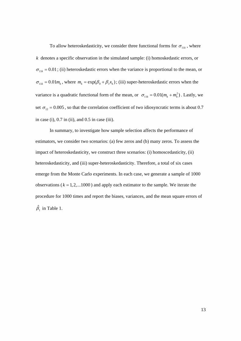
To allow heteroskedasticity, we consider three functional forms for 11k , where
k denotes a specific observation in the simulated sample: (i) homoskedastic errors, or
11 0.01k ; (ii) heteroskedastic errors when the variance is proportional to the mean, or
11 0.01k km , where 0 1exp( )k km x ; (iii) super-heteroskedastic errors when the
variance is a quadratic functional form of the mean, or 211 0.01( )k k km m . Lastly, we
set 12 0.005 , so that the correlation coefficient of two idiosyncratic terms is about 0.7
in case (i), 0.7 in (ii), and 0.5 in case (iii).
In summary, to investigate how sample selection affects the performance of
estimators, we consider two scenarios: (a) few zeros and (b) many zeros. To assess the
impact of heteroskedasticity, we construct three scenarios: (i) homoscedasticity, (ii)
heteroskedasticity, and (iii) super-heteroskedasticity. Therefore, a total of six cases
emerge from the Monte Carlo experiments. In each case, we generate a sample of 1000
observations ( 1,2,...1000k ) and apply each estimator to the sample. We iterate the
procedure for 1000 times and report the biases, variances, and the mean square errors of
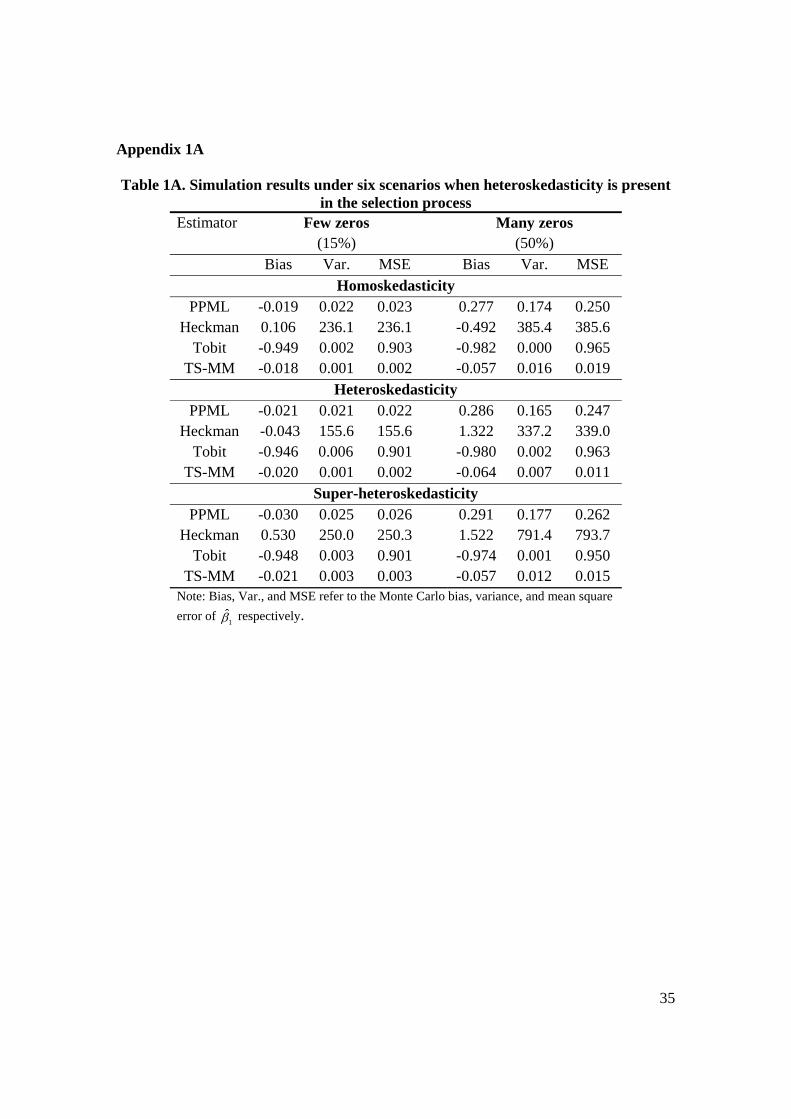
Note: Bias, Var., and MSE refer to the Monte Carlo bias, variance, and mean square
error of 1 respectively.
15
We discuss the performance of each estimator in turn. As shown in Table 1, the
PPML estimate of 1 is biased upward by 9% when zeros are few, and by more than
40% when zeros are prevalent. The reason is that, without differentiating the extensive
margin from the intensive margin, the PPML estimate co-finds the effect through 1 and
the effect through 1 . The problem becomes more evident when the portion of zeros
increases, as the extensive margin of trade plays a greater role. This finding echoes
Martin and Pham (2008) in that the PPML estimates can be severely biased when trade
data is limitedly dependent and zeros are frequent. Nevertheless, the PPML estimates are
fairly stable across different heteroskedastic patterns, as claimed in SST.
Three features are worth noting in the Heckman estimates. First, the Heckman
estimates are generally biased, due to the logarithmic transformation of trade flows. The
magnitude of the bias ranges from -4% in the case of few zeros and super-
heteroskedasticity to over 70% in the case of many zeros and heteroskedasticity. Second,
the Heckman estimates are not robust to heteroskedasticity. In either the case of few
zeros or many zeros, the Heckman estimate varies a lot as the variance structure of the
error term changes. Thirdly, the variances of the Heckman estimates are large in all cases,
illustrating the identification problem of the Heckman model in the absence of an
excluded variable. A glance at the E.T.-Tobit models reveals that the associated estimates
are severely biased in all scenarios, as found in SST.
Now we discuss the performance of the proposed TS-MM estimator. Table 1
suggests that the TS-MM estimate is reasonably accurate, with the bias around 2% when
zeros are few, and 7% when zeros are many. In other words, the TS-MM estimator
satisfactorily addresses the issue of sample selection. Moreover, the TS-MM estimate is
16
robust to various degrees of heteroskedasticity, as evidenced by the stability of bias and
variance across different heteroskedastic patterns. In fact, by the criteria of either the
magnitude of bias or mean squared error, the TS-MM estimator strictly dominates the
PPML estimator, the Heckman sample selection model, or the E.T.-Tobit model.
Several robustness checks are warranted for the Monte Carlo experiments. One
legitimate question is whether the TS-MM estimator is robust to heteroskedasticity in the
stage of selection as well. To address this concern, we conduct another set of Monte-
Carlo experiments in which we replace 22 0.005k with 22 0.01k km (so that the
variance of the error term in the selection equation increases with x ). The associated
results, reported in Appendix 1A, suggest that the TS-MM estimator again outperforms
the alternatives. Another interesting scenario worth considering is when the two margins
of trade work in opposite directions. For example, one can think of technical barriers,
which might increase the market shares of larger and capital-abundant exporters, while
driving out smallholder exporters who can barely meet the regulations. In this case, we
expect the PPML estimates, which co-find the two margins, to be biased downward. To
test the hypothesis, we conduct another set of experiments in which we set 1 0.05 .13
The associated results, reported in Appendix 1B, confirm that the PPML model delivers
attenuated results, while the TS-MM model remains outperforming all other alternatives.
We conclude from the Monte Carlo experiments that the proposed TS-MM model
outperforms the alternatives when the underlying data generating process follows the
system (2a)-(2d), because it simultaneously deals with both sample selection and
heteroskedasticity.
13 To maintain the same proportions of zeros, we set
0 0.125 and 0 0.05 for the case of few zeros
and many zeros respectively.
17
4. The Model Selection Strategy
In practice, however, the true data generating process is barely known to
researchers. Therefore, one has to explore whether sample selection is a concern and to
what degree heteroskedasticity matters for a particular application. To guide applied
work, we suggest a model selection strategy that allows one to choose the most
appropriate estimator.
Our proposed model selection strategy starts with screening various estimators
based on their economic and statistical properties. Specifically, we focus on each
estimator’s capability in dealing with zeros, accommodating heteroskedasticity, and
addressing sample selection. It is worth noting that the concern of heteroskedasticity is
closely related to the functional form in which the gravity equation is specified, i.e.,
whether trade flows ought to be characterized in levels, or in their logarithmic scales.
Given the right specification, heteroskedasticity is less of a concern for statistical
inferences if we use the heteroskedasticity-consistent standard errors. Therefore, the issue
with heteroskedasticity translates into the choice between the specification in levels and
the one in logs. The sample selection issue, in the context of trade, is closely related to
the identification of the two margins of trade. That is, the two margins of trade can be
told apart only when the sample selection is properly addressed.
Table 2 summarizes the strengths and weaknesses of commonly used estimators
for the gravity equation model. We argue that one can eliminate the Truncated OLS
estimator and the E.T.-Tobit model from the pool of candidate estimators. First, the
Truncated OLS estimator is inferior to other alternatives because it fails to accommodate
18
zeros at all. Second, the E.T.-Tobit model is dominated by the Heckman sample selection
model. The reason is that, although similar to the Heckman model in many aspects (as
shown in Table 2), The E.T.-Tobit model imposes a common threshold for all countries
to jump (Eaton and Tamura, 1994), which is at odds with the fact that fixed costs of trade
vary a lot across countries (Anderson and van Wincoop, 2004). Therefore, the evaluation
of the economic and statistical properties of estimators leads to a candidate pool of three
competing estimators: the PPML estimator, the Heckman sample selection model, and
the TS-MM estimator.
19
Table 2. Advantages and disadvantages of various estimators Estimator Zeros? In levels?
(robust to heteroskedasticity) Two margins? (sample selection)
Trun-OLS no no no PPML yes yes no Heckman yes no yes E.T.-Tobit yes no yes TS-MM yes yes yes
20
The second-round selection involves two statistical tools. First, we focus on the
sample selection issue and compare the Heckman model with the TS-MM model. While
both models correct for the potential sample selection bias, the TS-MM model differs
from the Heckman model in that, in the second-stage estimation, it characterizes trade in
levels, as opposed to in logarithmic scales. The MacKinnon-White-Davidson (MWD) test
can be used to choose between the specification in levels and the one in logs
(MacKinnon, White, and Davidson, 1983). Intuitively, the MWD test works as follows.14
We fit both the TS-MM model and the Heckman model and generate predicted trade
flows in the second stage. Denoting the series of predicted trade from the TS-MM model
and the Heckman model as M and N respectively, we run the second stage of the TS-
MM model again with an additional explanatory variable ˆ ˆln( )M N . We reject the null
hypothesis that the TS-MM model is correctly specified if the auxiliary variable is
statistically significant.15 Therefore, the MWD test results enable us to choose a preferred
model between the Heckman model and the TS-MM model.
The sample selection bias, as revealed by the model that survives the MWD test,
may or may not be statistically significant. In case the sample selection is an issue indeed,
we conclude from the model selection strategy that the model wins the MWD test is the
most appropriate model. On the other hand, if the sample selection bias is insignificant,
we need to further compare the model that wins the MWD test with the PPML model.
The reason is that, in the absence of sample selection, the PPML model might perform
14 Interested readers are referred to MacKinnon, White, and Davidson (1983) and Gujarati (2004) for more discussions. 15
One can also test the Heckman model against the TS-MM model by fitting the second stage of Heckman with an additional variable ˆ ˆexp( )M N . The null hypothesis that the Heckman model is correctly
specified is rejected if the auxiliary variable is statistically significant.
21
well in estimating the overall marginal effects. We use the Theil’s inequality coefficient,
as a measure of goodness-of-fit, to compare the two models. Specifically, the Theil’s
inequality coefficient is computed as
2 2 2ˆ ˆ( ) ( )i i i ii i i
TU y y y y ,
where y and y denote the observed and predicted trade flows respectively.16 The Theil’s
inequality coefficient lies between 0 and 1, with a smaller value indicating a better
goodness-of-fit. Therefore, in the absence of sample selection, the most appropriate
model is either the PPML model or the model that wins the MWD test, depending on
which fits the data better. The decision tree in Figure 1 summarizes the model selection
strategy.
16 For the PPML model, the predicted trade is computed as ˆexp( )X . For the TS-MM model, the
predicted trade is computed as ˆ ˆ ˆ( ) (exp( ) )Z X . For the Heckman model, the predicted trade is
computed ˆ ˆ ˆ( ) exp( )Z X .
22
Figure 1. Decision tree for the model selection strategy
23
5. An Empirical Application
We illustrate how the proposed TS-MM estimator and the model selection
strategy work by investigating world trade in 1990. The data come from SST. We have
aggregate bilateral trade records among 136 countries in the year 1990. Among the 18360
(=136*135) observations, 48% are zeros. The explanatory variables include the
geographic distance, the border dummy variable, the common language dummy variable,
the colonial tie, and the FTA dummy variable. As in Anderson and van Wincoop (2003),
we include both the importers’ fixed effects and the exporters’ fixed effects in the
regression analysis to control for the multi-lateral trade resistance terms.17
Following the model selection strategy, we restrict our attention to the three
competing estimators: the PPML model, the Heckman sample selection model, and the
TS-MM model. We expect two countries further apart to trade less. On the other hand,
we speculate that the volume of trade is larger if the two countries share a country border,
or use a common language, or had a colonial relationship, or engage in a regional trade
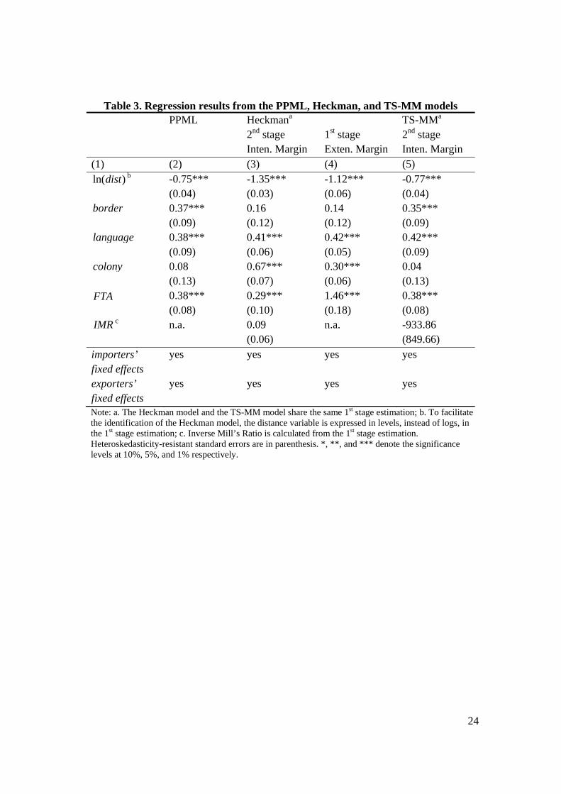
agreement. Table 3 presents the econometric results from all three models.
17
Due to the cross-sectional nature of the data, all country-specific characteristics (such as income, population, and remoteness) are subsumed into the exporters’ and importers’ fixed effects.
24
Table 3. Regression results from the PPML, Heckman, and TS-MM models PPML Heckmana TS-MMa 2nd stage
Inten. Margin 1st stage Exten. Margin
2nd stage Inten. Margin
(1) (2) (3) (4) (5) ln( )dist b -0.75***
(0.04) -1.35*** (0.03)
-1.12*** (0.06)
-0.77*** (0.04)
border 0.37*** (0.09)
0.16 (0.12)
0.14 (0.12)
0.35*** (0.09)
language 0.38*** (0.09)
0.41*** (0.06)
0.42*** (0.05)
0.42*** (0.09)
colony 0.08 (0.13)
0.67*** (0.07)
0.30*** (0.06)
0.04 (0.13)
FTA 0.38*** (0.08)
0.29*** (0.10)
1.46*** (0.18)
0.38*** (0.08)
IMR c n.a.
0.09 (0.06)
n.a. -933.86 (849.66)
importers’ fixed effects
yes yes yes yes
exporters’ fixed effects
yes yes yes yes
Note: a. The Heckman model and the TS-MM model share the same 1st stage estimation; b. To facilitate the identification of the Heckman model, the distance variable is expressed in levels, instead of logs, in the 1st stage estimation; c. Inverse Mill’s Ratio is calculated from the 1st stage estimation. Heteroskedasticity-resistant standard errors are in parenthesis. *, **, and *** denote the significance levels at 10%, 5%, and 1% respectively.
25
The PPML estimates, shown in Column (2) of Table 3, replicate the results
reported in SST. All explanatory variables bear the expected signs and all are statistically
significant except for the colonial tie dummy variable. Noticeably, since the PPML model
co-finds the two margins of trade, the estimated raw coefficients can be interpreted as the
overall marginal effects. Column (4) of Table 3 reports the first-stage estimation from the
Probit model, which is shared between the Heckman model and the TS-MM model.
Instead of presenting the estimated raw coefficients, we report the marginal effects on the
extensive margins of trade, as defined in (3b), after fitting the Probit model. Interestingly,
while all other trade determinants affect the propensity to trade in ways we anticipate, a
common country border does not seem to increase the likelihood of trade significantly.
The second-stage estimation of the Heckman model, as shown in Column (3) of Table 3,
reinforces this finding by showing contiguity does not matter for the size of trade either.
Additionally, since the sample selection bias is not statistically significant in the
Heckman model, the estimated raw coefficients in the second stage directly translate into
the marginal effects on the intensive margins of trade.
Turning to the second-stage estimation of the TS-MM model, or Column (5) of
Table 3, we find that the sample selection bias is not statistically significant either.
Hence, the estimated raw coefficients can be interpreted as the marginal effects on the
intensive margins of trade, as defined by (4b). Compared to the Heckman estimates, the
results from the second-stage TS-MM estimation suggest that countries sharing borders
trade more, but that countries with historical colonial ties do not trade significantly more
(although they are more likely to trade).
26
The difference in statistical and economic inferences across three models calls for
diagnostic analysis. Following the proposed model selection strategy, we first deal with
the sample selection issue and choose one between the Heckman model and the TS-MM
model. Specifically, we conduct two WMD tests to guide the choice of the specification
for the gravity equation (i.e., whether trade flows should be modeled in levels or in their
logarithmic scales). As shown in Table 4, the first WMD test is under the hypothesis that
the Heckman model is correctly specified, or, the logarithmic transformation can be taken
to the gravity equation; whereas the second one tests the TS-MM model against the
Heckman model. The associated P values of the WMD tests suggest that the TS-MM
model is preferred over the Heckman model.
27
Table 4. MWD test results and Theil’s indices The MWD tests P value H0: the 2nd stage of Heckman is correctly specified 0.00 H0: the 2nd stage of TS-MM is correctly specified 0.16
Goodness of fit Theil’s inequality coefficients PPML 0.14 TS-MM 0.14
28
However, the insignificance of the sample selection bias in the TS-MM model
compels us to further compare the TS-MM model with the PPML model. Coincidently,
the associated Theil’s inequality coefficients in Table 4 suggest that the TS-MM model
and the PPML model fit the data equally well. Nevertheless, we consider the TS-MM
model weakly preferred over the PPML model because it sheds light on the two margins
of trade.
In summary, applying the proposed model selection strategy, we find that the TS-
MM model is the most appropriate estimator. Next, we discuss the economic implications
of the TS-MM estimates. The elasticity of distance is of the magnitude -1.89(=-1.12-
0.77), more than doubling the effect reported in SST.18 In terms of the border effect, our
finding reinforces Anderson and van Wincoop (2003) in that a shared border enlarges the
size of trade by nearly 30%. While the colonial tie fosters trade primarily through the
extensive margin, a common language increases both the chance and size of trade. In
addition, regional trade agreements not only enhance pre-existing trade by 38% (which is
compatible with the result reported by Baier and Bergstrand (2007)), but also
significantly improves market access.19
6. Conclusion
A vexing issue in the gravity equation model is its statistical estimation in the
presence of two stylized features of trade data: sample selection and heteroskedasticity.
We contribute to empirical applications of the gravity equation model in two important
ways. First, we propose a Two-Step Method of Moments (TS-MM) estimator that deals 18
Nevertheless, the distance effect we find is within the range reported by Disdier and Head (2008). 19
Similarly, Felbermayr and Kohler (2006) show that the WTO membership facilitates international trade primarily via the extensive margin.
29
with both issues. The novel estimator works as follows. In the first step, the estimator
explains why trade takes place at all and sheds light on the extensive margin of trade. In
the second step, the volumes of trade are characterized, in levels, by an augmented
gravity equation with correction for the sample selection bias. The method of moments
technique delivers consistent estimates regardless of heteroskedastic patterns. Our second
contribution is the provision of a model selection strategy, which allows one to choose
the most appropriate estimator in practice. In particular, we show how economic theories
and statistical tools can be used together to guide the estimation of a gravity model.
Several extensions are worth attempting for future research. For instance, the
identification of different sources of zeros is of great relevance: while some zero trade
records are due to the inability to trade, others may reflect missing data entries. Further,
the TS-MM estimator can be applied to other constant-elasticity models, such as the
Mincer’s earnings model (Mincer, 1974), where sample selection and heteroskedasticity
might be of concern.
30
Reference
Anderson, J. E., “A Theoretical Foundation for the Gravity Equation,” American
Economic Review 69 (1979), 106-116.
Anderson, J. E., “The Gravity Model,” NBER Working Papers 16576, National Bureau
of Economic Research, Inc. (2010).
Anderson, J. E., and E. van Wincoop, “Gravity with Gravitas: A Solution to the Border
Puzzle,” American Economic Review 93 (2003), 170-192.
Anderson, J. E., and E. van Wincoop, “Trade Costs,” Journal of Economic Literature 42
(2004), 691-751.
Arkolakis, C., “Market Penetration Costs and the New Consumers Margin in
International Trade,” Journal of Political Economy 118 (2010), 1151-1199.
Baier, S. L., and J. H. Bergstrand, “Do Free Trade Agreements Actually Increase
Members' International Trade?” Journal of International Economics, 71 (2007),
72-95.
Baldwin, R., and D. Taglioni, “Gravity for Dummies and Dummies for Gravity
Equations,” NBER Working Papers 12516, National Bureau of Economic
Research, Inc. (2006).
Bergin, P. R., and C.-Y. Lin, “Exchange Rate Regimes and the Extensive Margin of
Trade,” NBER Chapters, in: NBER International Seminar on Macroeconomics
(pp. 201-227), National Bureau of Economic Research, Inc. (2008).
Bergstrand, J. H., “The Gravity Equation in International Trade: Some Micro-economic
Foundations and Empirical Evidence,” Review of Economics and Statistics 67
(1985), 471-481.
31
Bergstrand, J. H., “The Generalized Gravity Equation, Monopolistic Competition, and the
Factor-Proportions Theory in International Trade,” Review of Economics and
Statistics 71 (1989), 143-153.
Besedes, T., and T. J. Prusa, “The Role of Extensive and Intensive Margins and Export
Growth,” Journal of Development Economics 96 (2011), 371-379.
Burger, M., F. van Oort, and G.-J. Linders, “On the Specification of the Gravity Model of
Trade: Zeros, Excess Zeros and Zero-inflated Estimation,” Spatial Economic
Analysis, 4 (2009), 167-190.
Chaney, T., “Distorted Gravity: The Intensive and Extensive Margins of International
Trade,” The American Economic Review 98 (2008), 1707-1721.
Chang, T., and P. S. Kott, “Using Calibration Weighting to Adjust for Nonresponse under
a Plausible Model,” Biometrika, 95 (2008), 555-571.
Deardorff, A., “Determinant of Bilateral Trade: Does Gravity Work in a Neoclassical
World?” in J. Frankel (Eds.), The Regionalization of the World Economy.
(Chicago: University of Chicago Press, 1998).
Disdier, A.-C., and K. Head, “The Puzzling Persistence of the Distance Effect on
Bilateral Trade,” Review of Economics and Statistics 90 (2008): 37-48.
Eaton, J., and A. Tamura, “Bilateralism and Regionalism in Japanese and U.S. Trade and
Direct Foreign Investment Patterns,” Journal of the Japanese and International
Economies 8 (1994), 478-510.
Evenett, S. J., and W. Keller, “On Theories Explaining The Success Of The Gravity
Equation,” Journal of Political Economy 110 (2002), 281-316.
32
Feenstra, R. C., J. R. Markusen, and A. K. Rose, “Using the Gravity Equation to
Differentiate among Alternative Theories of Trade,” The Canadian Journal of
Economics 34 (2001), 430-447.
Felbermayr, G. J., and W. Kohler, “Exploring the Intensive and Extensive Margins of
World Trade,” Review of World Economics 142 (2006), 642-674.
Grant, J., and K. A. Boys, “Agricultural Trade and the GATT/WTO: Does Membership
Make a Difference,” The American Journal of Agricultural Economics 94 (2012),
1-24.
Gujarati, D. Basic Econometrics, 4th edition, pp. 280-282, (New York: The McGraw-Hill
companies, 2004).
Heckman, J. J. “Sample Selection Bias as a Specification Error,” Econometrica, 47
(1979), 153-161.
Helpman, E., M. Melitz, and Y. Rubinstein. “Estimating Trade Flows: Trading Partners
and Trading Volumes,” The Quarterly Journal of Economics, 123 (2008), 441-
487.
Hummels, D., and P. J. Klenow, “The Variety and Quality of a Nation's Exports,”
American Economic Review 95 (2005), 704–723.
Little R. J. A., and D.B. Rubin, Statistical Analysis with Missing Data. (New York: John
Wiley & Sons, 1987).
MacKinnon, J., H. White, and R. Davidson, “Tests for Model Specification in the
Presence of Alternative Hypothesis; Some Further Results.” Journal of
Econometrics 21 (1983), 53–70.
33
Maddala, G. S., Limited-Dependent and Qualitative Variables in Econometrics,
(Cambridge: Cambridge University Press, 1986).
Markusen, J. R., “Explaining the Volume of Trade: An Eclectic Approach,” The
American Economic Review 76 (1986), 1002-1011.
Martin, W., and C. S. Pham, “Estimating the Gravity Model When Zero Trade Flows are
Frequent,” Economics Series 2008, Deakin University, Faculty of Business and
Law, School of Accounting, Economics and Finance. (2008).
Melitz, M. J. “The Impact of Trade on Intra-Industry Reallocations and Aggregate
Industry Productivity,” Econometrica 71 (2003), 1695-1725.
Mincer, J., Schooling, Experience, and Earnings, (New York: NBER Press, 1974).
Novy, D., “International Trade Without CES: Estimating Translog Gravity,” CEP
Discussion Papers. (2010).
Puhani, P., “The Heckman Correction for Sample Selection and its Critique,” Journal of
Economic Surveys 14 (2000), 53-68.
Ranjan, P., and J. L. Tobias, “Bayesian Inference for the Gravity Model,” Journal of
Applied Econometrics 22 (2007), 817–838.
Santos Silva, J. M. C., and S. Tenreyro. “The Log of Gravity,” Review of Economics and
Statistics 88 (2006), 641-658.
Santos Silva, J. M.C., and S. Tenreyro. “Further Simulation Evidence on the Performance
of the Poisson Pseudo-Maximum Likelihood Estimator,” Economic Letters 112
(2011), 220-222.
Shepherd, B., “Geographic Diversification of Developing Country Exports,” World
Development 38 (2010), 1217-1228.
34
Sun, L., and M. R. Reed, “Impacts of Free Trade Agreements on Agricultural Trade
Creation and Trade Diversion,” The American Journal of Agricultural Economics
92 (2010), 1351-1363.
Theil H., Economic Forecasts and Policy, Second Revised Edition, (Amsterdam: North-
Holland Publishing Company, 1961).
Tinbergen, J., “Les Données Fondamentales d'un Plan Régional,” Revue Tiers Monde, 3
(1962), 329-336.
White, H., “A Heteroskedasticity-Consistent Covariance Matrix Estimator and a Direct
Test for Heteroskedasticity,” Econometrica 48 (1980), 817-838.
35
Appendix 1A
Table 1A. Simulation results under six scenarios when heteroskedasticity is present in the selection process


![Estimating and interpreting structural equation models … · Estimating and interpreting structural equation models in Stata 12 ... and Var [ǫ] = Σ sem (y1 ... Structural equation](https://static.documents.pub/doc/80x56/5b286e167f8b9ae8108b4592/estimating-and-interpreting-structural-equation-models-estimating-and-interpreting.jpg)


