ESTIMATION OF MULTIVARIATE PROBIT MODELS VIA BIVARIATE PROBIT
John Mullahy
Working Paper 21593http://www.nber.org/papers/w21593
NATIONAL BUREAU OF ECONOMIC RESEARCH1050 Massachusetts Avenue
Cambridge, MA 02138September 2015
I would like to thank Bill Greene, Stephen Jenkins, João Santos Silva, and an anonymous reviewerfor helpful comments on earlier drafts. Support has been provided by NICHD Grant P2CHD047873to UW-Madison's Center for Demography and Ecology and by the RWJF Health & Society ScholarsProgram at UW-Madison. The views expressed herein are those of the author and do not necessarilyreflect the views of the National Bureau of Economic Research.
NBER working papers are circulated for discussion and comment purposes. They have not been peer-reviewed or been subject to the review by the NBER Board of Directors that accompanies officialNBER publications.
Estimation of Multivariate Probit Models via Bivariate ProbitJohn MullahyNBER Working Paper No. 21593September 2015JEL No. C3,I1
ABSTRACT
Models having multivariate probit and related structures arise often in applied health economics. Whenthe outcome dimensions of such models are large, however, estimation can be challenging owing tonumerical computation constraints and/or speed. This paper suggests the utility of estimating multivariateprobit (MVP) models using a chain of bivariate probit estimators. The proposed approach offers twopotential advantages over standard multivariate probit estimation procedures: significant reductionsin computation time; and essentially unlimited dimensionality of the outcome set. The time savingsarise because the proposed approach does not rely simulation methods; the dimension advantage arisesbecause only pairs of outcomes are considered at each estimation stage. Importantly, the proposedapproach provides a consistent estimator of all the MVP model's parameters under the same assumptionsrequired for consistent estimation based on standard methods, and simulation exercises suggest noloss of estimator precision.
John MullahyUniversity of Wisconsin-MadisonDept. of Population Health Sciences787 WARF, 610 N. Walnut StreetMadison, WI 53726and [email protected]
A data appendix is available at:http://www.nber.org/data-appendix/w21593
1
1. Introduction
Models having multivariate probit and related structures arise often in applied
health economics (see Mullahy, 2011, for references). When the outcome dimensions of
such models are large, however, estimation can be challenging owing to numerical
computation constraints and/or speed.
This paper suggests the utility of estimating multivariate probit (MVP) models using
a chain of bivariate probit estimators. It will be seen that the proposed approach, based on
Stata's biprobit and suest procedures and driven by a Mata function bvpmvp(...), affords two
potential advantages over Stata's mvprobit procedure: significant reductions in
computation time; and essentially unlimited dimensionality of the outcome set (mvprobit's
limit is M=20 outcomes).1 The time savings arise because, unlike mvprobit, bvpmvp(...) does
not rely simulation methods; the dimension advantage arises because only pairs of
outcomes are considered at each estimation stage. Importantly, the proposed bvpmvp(...)
approach provides a consistent estimator of all the MVP model's parameters under the
same assumptions required for consistent estimation via mvprobit, and simulation
exercises reported below suggest no loss of estimator precision relative to mvprobit.
The approach suggested here was inspired by the goal of embedding MVP
estimation in a large-‐replication bootstrap exercise. The simulation results presented in
Section 5 suggest that the computation time savings afforded by the bvpmvp(...) method
relative to mvprobit can be significant while numerical differences in the respective point
1 Stata SE's restriction that matsize cannot exceed 11,000 ultimately places a limit on the size of the parameter vector that can be estimated. All references to Stata herein are to Stata/SE, Version 13.1. Whether the results obtained here using Stata generalize to other statistical packages is an open question.
2
estimates and estimated standard errors are trivial. Since the potential applicability of
MVP models is broad, it is valuable in practice that such potential not be thwarted by
computational challenges.
The plan for the remainder of the paper is as follows. Section 2 describes the MVP
model. Section 3 describes the bvpmvp(...) method. Section 4 describes the comparison
where i=1,...,N indexes observations, j=1,...,M indexes outcomes, xi is a K-‐vector of
exogenous covariates, the ui are assumed to be iid independent across i but correlated
across j for any i, and "MVN" denotes the multivariate normal distribution. (Henceforth the
"i" subscripts will be suppressed.) The standard normalization sets the diagonal elements
of R equal to 1 so that R is a correlation matrix with off-‐diagonal elements !ρpq ,
3
! p,q{ }∈ 1,...,M{ } , !p≠ q .2 With standard full rank conditions on the x's and each !ρpq <1
then !!B = β1 ,...,βM⎡⎣ ⎤⎦ and R will be identified and estimable with sufficient sample variation
in the x's.
3. Estimation and Inference
Estimation of the M-‐outcome multivariate probit model using mvprobit requires
simulation of the MVN probabilities (Cappellari and Jenkins, 2003), with mvprobit
computation time increasing in M, K, N, and simulation draws (D).3 It turns out, however,
that all the parameters (B,R) can be estimated consistently using bivariate probit -‐-‐
implemented as Stata's biprobit procedure -‐-‐ while consistent inferences about all these
parameters are afforded via Stata's suest procedure. Since the proposed approach will be
seen to be significantly faster in terms of computation time with no obvious disadvantages,
this strategy may merit consideration in applied work.
The key result for the proposed estimation strategy is that the multivariate normal
distribution is fully characterized by the mean vector xB and correlation matrix R. For
present purposes, the key feature of the multivariate (conditional) normal distribution
2 This normalization rules out cases like heteroskedastic errors (Wooldridge, 2010, section 15.7.4). While this normalization is common -‐-‐ normalizing each univariate marginal to be a standard probit, for instance -‐-‐ it is not the only possible normalization of the covariance matrix. 3 Specifically, in the empirical exercises reported below as well as in some other simulations not reported here, it is found that mvprobit computation time increases: trivially in K; essentially proportionately in D; slightly more than proportionately in N; and at a rate between 2M and 3M in M. Greene and Hensher, 2010, suggest that MVP computation time would increase with 2M but the results obtained in the simulations undertaken here suggest a somewhat greater rate of increase.
4
!!F y1* ,...,yM* x( ) is that all its bivariate marginals !!F yj* ,ym* x( ) are bivariate normal with mean vectors and correlation matrixes corresponding to the respective submatrixes of xB and R
(Rao, 1973, 8a.2.10).
Under the normalization that the diagonal elements of R are all one, the B
parameters are identified based on knowledge of all M (conditional) univariate marginals
!!F yj* x( ) ; there is no need to appeal to the multivariate features of !!F y1* ,...,yM* x( ) to identify B. The .5M(M-‐1) bivariate marginals provide the additional information about the !ρpq
parameters. As such, identification of the parameters of all the bivariate marginals implies
identification4 of the parameters of the full multivariate joint distribution so that consistent
estimation of all the bivariate marginal probit models !!Pr yp = tp ,yq = tq x( ) provides consistent estimates of all the parameters !! B,R( ) of the full multivariate probit model
weighted average of consistent estimators is in general a consistent estimator, the resulting
! !BA! will itself be consistent for B. This averaging arises because the B parameters in the
proposed approach are overidentified, i.e. there are M-‐1 consistent estimates of each !β j ,
j=1,...,M. One could use some other rule to compute a single consistent estimate of each !β j
from among the M-‐1 candidates, but unless alternative strategies could boast significant
precision gains, computational simplicity recommends the simple average as an obvious
5 biprobit estimates directly the inverse hyperbolic tangent of !ρpq or
!.5ln 1+ρpq( ) 1−ρpq( )( ) . 6 α! and Ω
! are the suest stored matrix results e(b) (a row vector) and e(V), respectively.
6
solution. See the Appendix for further discussion.
Finally, let Q denote the !.5M M−1( ) vector of the !tanh−1 ρjk( ) estimated in each
biprobit specification, and define the !M .5 M−1( )+K( )×1 vector ! !Θ! = vec BA
"( )T ,Q!T⎡
⎣⎢⎢
⎤
⎦⎥⎥
T.
Define H as the !M .5 M−1( )+K( )×M M−1( ) .5+K( ) averaging and selection matrix that maps
α! to Θ! , i.e. ! !Θ! =Hα!
T; the elements of H are 1/(M-‐1), one, or zero.7 The estimated
variance-‐covariance matrix of Θ! , useful for inference, is given by
! !var! Θ"( ) =HΩ"HT .
bvpmvp(...): A Mata Function to Implement the Proposed Estimation Approach
The function bvpmvp(...) returns the !M k + .5 M−1( )( )× M k + .5 M−1( )( )+1( ) matrix
whose first column is ! Θ!T
and whose remaining elements are the
!M k + .5 M−1( )( )'dimension symmetric square matrix ! var! Θ"( ) . bvpmvp(...) takes six
arguments: (1) a string containing the names of the M outcomes; (2) a string containing the 7 A general form of the H matrix is complicated to express concisely. As an example, for M=3 and K=2 the !9×15 H matrix, computed internally by bvpmvp(...), is
For mvprobit, the draws(.) option was set both at 10 and 20. The simulations are
performed using Stata/SE Version 13.1 on an iMac 3.4GHz Intel Core i7 processor and OS X
v10.8.8.
5. Simulation Results
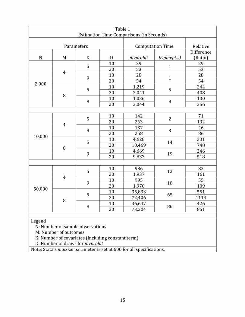
Key results of the simulations are summarized in Tables 1-‐3. Table 1 displays the
absolute and relative computation times for mvprobit and bvpmvp(...) estimation across the
various combinations of the N, M, K, and D parameters. Enormous differences in
computation time are seen between the two estimation methods across all the different
parameter combinations (for reference, it may be useful to recall that there are 86,400
seconds in one day). Tables 2 and 3 present a side-‐by-‐side comparison of the point
estimates of B and R obtained in one select specification (N=10,000, M=4, K=5). For both B
and R the differences between the mvprobit and bvpmvp(...) point estimates and
8 The simulations set Stata's matsize parameter at 600 for all specifications. In some preliminary investigation, it was observed that computation time for bvpmvp(...) increased significantly when matsize was set much larger than necessary; this was not the case for mvprobit.
9
corresponding estimated standard errors are trivial.
In light of these results, use of methods like bvpmvp(...) to estimate MVP models
merits consideration when computation time is an important consideration.9
6. Multivariate Ordered Probit Models
Analogous conceptual considerations arise in the context of multivariate ordered
probit (MVOP) models in which the observed ordered outcomes are !yoj∈ 0,...,Gj{ } for finite integers !Gj ≥1 . MVOP modeling involves estimation of and inference about the parameters
B and R as well as the vector of category cutpoints, C (for each outcome yoj there are Gj
cutpoints that delineate the Gj+1 categories).10
9 It should be noted that these simulations paint what is in some sense a "worst-‐case" picture for mvprobit estimation. The simulations use mvprobit "out of the box," i.e. without specifying any options that might enhance estimation speed (see the Stata "help" file for mvprobit and also Cappellari and Jenkins, 2003 and 2006). For instance, specifying a smaller number of draws (e.g. draws(3) or draws(5)) would clearly result in faster estimation times; any diminished performance of the mvprobit estimator relative to the performance at greater number of draws would be a potential consideration, however. Alternatively, using good starting values for R via mvprobit's atrho0(.) option might also be expected to result in faster estimation times. One such approach would involve two stages: (1) estimate the full model using mvprobit with a small number of draws, e.g. draws(1) or draws(2); and (2) use the estimate of R thus obtained to provide starting values for a second mvprobit estimation with a larger number of draws (e.g. draws(10) or draws(20)) being specified. This approach -‐-‐ with draws(1) specified initially, followed by draws(10) -‐-‐ was examined in some simulations. It was observed in this instance that the two-‐stage approach resulted in roughly a 10% reduction in overall estimation time, due mainly to a smaller number of iterations (three vs. four) required for convergence in the second stage. This paper also has not considered how estimation using Stata's cmp procedure to estimate the MVP model would compare with the bvpmvp(...) approach. I would like to thank Stephen Jenkins and an anonymous referee for their insights and suggestions on these matters. 10 For the MVOP model B will not contain a parameter for the constant term since this is absorbed into the cutpoints C.
10
An estimation strategy fully analogous to bvpmvp(...) is not available since the
bioprobit procedure (Sajaia, 2008) does not permit postestimation prediction with the
score option, as required by suest. However, an alternative, fully consistent, and
computationally efficient approach is available, as follows. First, estimate M univariate
ordered probit models using Stata's oprobit procedure and store these results using
estimates store. This provides consistent estimates of the B and C parameters. Second,
estimate a chain of bivariate binary probit models using biprobit -‐-‐ as with bvpmvp(...) -‐-‐
and store these estimates using estimates store. This provides a consistent estimate of R.11
Note that any thresholds used to map the ordered yoij to their corresponding coarsened
binary outcomes should result in consistent estimates of R. biprobit uses the rule that a
nonbinary outcome is treated as zero for zero values and one otherwise; this is a
convenient mapping that minimizes programming burden. Third, combine all the
estimates stored in these two steps using suest. The estimates from suest can then be used
for inference. The do file containing the Mata code for the function bvopmvop(...) that
implements this approach is available with this paper's supplementary materials.12 An
example of bvopmvop(...) output is presented in Exhibit 2.13
11 Note that this also provides consistent estimates of B, but these are unnecessary given those obtained in the first step. 12 bvopmvop(...) accommodates ordered outcomes having different numbers of cutpoints, including mixed ordered and binary outcomes. The single cutpoint estimated in oprobit for binary outcomes is -‐1 times the corresponding constant term that would be estimated using probit. 13 The outcomes in this example are ordered versions yoj of the yj used in the earlier simulations in which the outcome value 2 is assigned if !1≤ yj
* ≤2 and 3 is assigned if !yj* >2 .
Then y2 combines the top two categories and y3 combines the top three categories (i.e. y3 is the original binary measure). Thus, the numbers of categories are G1=4, G2=3, G3=2, and G4=4.
11
7. Summary
This paper has presented a novel estimation strategy for consistent estimation of
and inference about the parameters of MVP and MVOP models. The straightforward
implementation of these approaches using available Mata programs recommends their
consideration in applied work, particularly in situations involving large numbers of
outcomes (M), large sample sizes (N), or in situations requiring repeated MVP estimation
like bootstrapping exercises.
In closing, it should be noted that the methods suggested here may prove useful in
many but not all applications of multivariate probit models. Ultimately the methods
proposed here -‐-‐ as well as the mvprobit method -‐-‐ permit estimation of the joint
conditional probability model !!Pr y = k x( ) for the M-‐vectors of outcomes y, all possible 2M
vectors k=[km], !km ∈ 0,1{ } , and exogenous covariates x. As such, when these joint conditional probabilities are per se the estimands of interest, when they are instrumentally
of interest in the estimation of other quantitites (see Mullahy, 2011, for discussion), or
when reduced forms of structural models are of interest, the approach suggested here may
prove useful. However in other MVN contexts with binary outcomes
-‐-‐ e.g. where endogenous ym are RHS variables in the structural models for other latent !yj*
-‐-‐ consistent estimation of the structural parameters will typically demand attention to the
full joint probability structure, not just its bivariate marginals.14
14 Thanks are owed to an anonymous reviewer for emphasizing these points.
12
References
Cappellari, L. and S.P. Jenkins. 2003. "Multivariate Probit Regression Using Simulated
Maximum Likelihood." Stata Journal 3: 278–294.
Cappellari, L. and S.P. Jenkins. 2006. "Calculation of Multivariate Normal Probabilities by
Simulation, with Applications to Maximum Simulated Likelihood Estimation." Stata
Journal 6: 156-‐189.
Greene, W.H. and D.A. Hensher. 2010. Modeling Ordered Choices: A Primer. Cambridge:
Cambridge University Press.
Mullahy, J. 2011. "Marginal Effects in Multivariate Probit and Kindred Discrete and Count
Outcome Models, with Applications in Health Economics." NBER W.P. 17588.
Rao, C.R. 1973. Linear Statistical Inference and Its Applications, 2nd Edition. New York:
Wiley.
Sajaia, Z. 2008. BIOPROBIT: Stata Module for Bivariate Ordered Probit Regression. Boston
College Department of Economics, Statistical Software Components, No. S456920.
Wooldridge, J.M. 2010. Econometric Analysis of Cross Section and Panel Data, 2nd Edition.
Cambridge, MA: MIT Press.
13
Appendix: Additional Remarks on Combining biprobit Estimates
In general, the optimal approach to combining such multiple estimates in the
overidentified case is to use a minimum-‐distance estimator with an optimal weight matrix
(Wooldridge, 2010, section 14.5). In the present context this would amount to computing a
weighted average for each point estimate, i.e. ! β! jkw = wjkmβ
!jkmm=1
m≠jM∑ , j=1,...,M, k=1,...,K.
Implementing the minimum-‐distance approach can be computationally challenging,
however. For example, consider the simplest case, M=3. The optimal (variance-‐
minimizing) weights even in this instance are complicated functions of the estimates'
variances and covariances; suppressing the j,k subscripts, for ! p,q,r{ }∈ 1,2,3{ } , !p≠ q ≠ r these optimal weights are:
where σ•• are variances and covariances of the parameter estimates (the empirical
counterpart, ! wr! , would use σ••
! ). The algebraic complexity of these weights increases
rapidly as M increases.
The considerable additional computational complexity involved in implementing
such a minimum-‐distance approach is unlikely to provide much benefit (in terms of
precision) unless the optimal wjkm were to diverge dramatically from 1/(M-‐1). The
simulations undertaken here suggest this is unlikely to be the case. In general the optimal
weights will diverge from the equi-‐weighted case of 1/(M-‐1) to the extent that the
variances and covariances of and between the parameter point estimates differ
substantively across the (M-‐1) estimates.15
15 Bill Greene suggested to me that a computationally straightforward middle-‐ground weighting strategy would be to, in essence, ignore the cross-‐estimator covariances and compute the variance-‐matrix-‐weighted quantities:
! β jv! = var! βm
!( )⎡⎣⎢
⎤⎦⎥−1
m=1m≠jM∑
⎡
⎣⎢⎢
⎤
⎦⎥⎥
−1× var! βm
!( )⎡⎣⎢
⎤⎦⎥−1βm!
m=1m≠jM∑ , j=1,...,M.
14
For illustrative purposes, selecting arbitrarily the (M-‐1) point estimates
corresponding to the parameter !β11 (outcome y1, covariate x1) for the N=10,000, M=8 and
K=5 specification, the range of the seven point estimates ! β11! is [.3266, .3288], the range of
the corresponding seven estimated point estimate variances is [.001983, .001995], and the
range of the 28 estimated point estimate covariances is [.001983, .001993]. It is thus
unlikely that the optimal weights would diverge much from 1/(M-‐1).
The ultimately important result is that at least insofar as the simulations conducted
for this paper are concerned, the differences between the mvprobit and bvpmvp(...) point
estimates and estimated standard errors are inconsequentially small (see Tables 2 and 3).
15
Table 1 Estimation Time Comparisons (in Seconds)
Parameters Computation Time Relative Difference (Ratio)
N M K D mvprobit bvpmvp(...)
2,000
4 5 10 29 1 29
20 53 53
9 10 28 1 28 20 54 54
8 5 10 1,219 5 244
20 2,041 408
9 10 1,036 8 130 20 2,044 256
10,000
4 5 10 142 2 71
20 263 132
9 10 137 3 46 20 258 86
8 5 10 4,628 14 331
20 10,469 748
9 10 4,669 19 246 20 9,833 518
50,000
4 5 10 986 12 82
20 1,937 161
9 10 995 18 55 20 1,970 109
8 5 10 35,833 65 551
20 72,406 1114
9 10 36,647 86 426 20 73,204 851
Legend N: Number of sample observations M: Number of outcomes K: Number of covariates (including constant term) D: Number of draws for mvprobit Note: Stata's matsize parameter is set at 600 for all specifications.
16
Table 2 mvprobit and bvpmvp(...) Comparison: !B
! and !BA! Point Estimates, One Example
(N=10,000, M=4, K=5; Estimated Standard Errors in Parentheses)
Outcome Covariate mvprobit (draws=20) bvpmvp(...)
y1
x1 0.3265 (.0448)
.3279 (.0446)
x2 -‐0.3301 (.0447)
-‐.3314 (.0447)
x3 0.3184 (.0447)
.3198 (.0449)
x4 -‐0.3902 (.0448)
-‐.3916 (.0447)
Constant 0.3901 (.0466)
.3909 (.0464)
y2
x1 -‐0.4487 (.0456)
-‐.4487 (.0455)
x2 0.5624 (.0458)
.5620 (.0456)
x3 -‐0.3998 (.0457)
-‐.3977 (.0457)
x4 0.4000 (.0456)
.3961 (.0457)
Constant -‐0.5086 (.0474)
-‐.5079 (.0474)
y3
x1 0.3102 (.0445)
.3151 (.0446)
x2 0.3846 (.0445)
.3875 (.0449)
x3 -‐0.3188 (.0446)
-‐.3206 (.0447)
x4 -‐0.3462 (.0446)
-‐.3496 (.0447)
Constant 0.3230 (.0463)
.3210 (.0463)
y4
x1 0.4567 (.0455)
.4573 (.0457)
x2 -‐0.4438 (.0455)
-‐.4408 (.0457)
x3 -‐0.4489 (.0456)
-‐.4516 (.0457)
x4 0.4555 (.0456)
.4499 (.0453)
Constant -‐0.4552 (.0472)
-‐.4524 (.0472)
17
Table 3
mvprobit and bvpmvp(...) Comparison: !R! Point Estimates, One Example
(N=10,000, M=4, K=5; Estimated Standard Errors in Parentheses) R
mvprobit (draws=20) bvpmvp(...)
!ρ12 .3190 (.0158)
.3308 (.0159)
!ρ13 .4942 (.0134)
.5073 (.0134)
!ρ14 .2766 (.0160)
.2872 (.0161)
!ρ23 .3356 (.0156)
.3424 (.0158)
!ρ24 .2000 (.0163)
.2034 (.0167)
!ρ34 .3059 (.0157)
.3086 (.0160)
18
Exhibit 1: Sample Output from bvpmvp(...) (N=10,000, M=4, K=5)