1

Evaluating the Hedging Effectiveness in Crude Palm Oil Futures Market during

Financial Crises

You-How Go

Faculty of Business and Finance, Universiti Tunku Abdul Rahman (UTAR),

Perak, Malaysia

E-mail address: goyh@utar.edu.my

Wee-Yeap Lau (Corresponding author)

Faculty of Economics and Administration, University of Malaya,

Kuala Lumpur, Malaysia.

E-mail address: wylau@um.edu.my

ABSTRACT

This study examines whether there is a significant change in hedging effectiveness on

Crude Palm Oil (CPO) futures market from January 1986 to December 2013. Eight

hedging models with different mean and variance-covariance specifications have been

evaluated. As the volatility of spot and futures markets is not similar across time, both

markets exhibit asymmetric information transmission. Our results of out-of-sample

evaluation show, firstly, the time-varying hedge ratios with basis term produce better

performance during both financial crises. Secondly, high dynamic hedge ratios during the

Asian financial crisis contribute to the support for CCC-GARCH model. Thirdly, during

global financial crisis, BEKK-GARCH model appears to provide more risk reduction as

compared to others. From the perspective of economic modeling, incorporating the basis

term in modeling the joint dynamics of spot and futures returns during the crises provide

better results. This study recommends that CPO market participants to adjust their

hedging strategies in response to different movement in market volatility.

Keywords: Generalized autoregressive conditional heterosedasticity (GARCH) model,

basis term, minimum-variance hedge ratios and hedging effectiveness.

JEL Classification: G12, G13, G14

2

1. Introduction

Being one of the world leading producers and exporters of palm oil, Malaysia alone

accounted for 39 per cent of world production and 45 per cent of world exports in 2011

based on the data released by the Malaysian Palm Oil Board (MPOB). Given the

prominence of this commodity to the economy, Malaysian crude palm oil (CPO) futures

market has been in existence in the Kuala Lumpur Commodity Exchange (KLCE) since

October 1980, and continued to be one of the active futures market for CPO related

derivative product in the world under the platform of Bursa Malaysia Derivative (BMD)

Berhad in 2003.

Like other market commodities, the price movement of CPO is subjected to

fluctuation throughout various economic climates. As observed in Figure 1, it shows that

CPO spot and futures returns have high volatility in three distinct periods which

correspond to the world economic recession in 1986, Asian financial crisis in 1997/1998

and global financial crisis in 2008/2009. Besides the global economic recession, which

happened during 1985-1987, Malaysian palm oil was subject to a series of adverse

publicity launched by the American Soybean Association. As a consequence, Malaysian

growth was halted abruptly as palm oil price had been halved.

In the aftermath of Asian financial crisis, the depreciation of Ringgit caused the

restructuring of the Malaysian derivative market to undergo a series of regulatory reform.

In response to this crisis, BMD’s CPO futures contracts were traded RM2,700 per tonne

at the Commodity and Monetary Exchange (COMMEX) in November 1998 (MPOB,

1998). Subsequently, palm oil has become the top foreign exchange earner, exceeding the

revenue derived from crude petroleum, petroleum products by a wide margin.

However, due to the La Nina effect in 2008, Malaysian palm oil export dropped from

RM13, 504 million tonnes in the third quarter to RM9, 271 million tonnes in the fourth

quarter of 2008 due to heavy rainfall and lower fresh fruit bunches (Central Bank

Malaysia, 2009). It was observed that CPO futures price also decreased from an average

of RM3506.12 in the first quarter of 2008 to RM1898.93 in first quarter of 2009. 1

Since the revival of China and India’s gross domestic production growth in 2009, the

total CPO futures contract traded has subsequently increased from 3,003,549 contracts in

2008 to 4,008,882 contracts in 2009 steadily with the rising of demand from both

countries.2 After recovery in the global economy in 2010, the rising of petroleum crude

oil has continually led to the increase of CPO price and directly reduced pricing volatility

after 2011.

The above account testifies that the price movement of CPO is uncertain and often

influenced by economic or environmental factors. Hence, to implement better hedging

strategies during economic downturn, there is a need among market participants to focus

on futures market as a means to minimize the risk of price fluctuation. However, there is

1 Based on data are extracted from Thomson DataStream on 12 January 2013

2 See the report of the United Nations Development Program (2009) at p. 68.

3

no conclusive evidence to state which model provides the best hedging performance

during extremely volatile economic periods. This study intends to revisit this issue and

extend earlier studies by using basis term in modeling the joint dynamics of spot and

futures returns.

0

0.05

0.1

0.15

0.2

0.25

0.3

0.35

0.4

0.45

0.5

1/6/

1986

1/6/

1988

1/6/

1990

1/6/

1992

1/6/

1994

1/6/

1996

1/6/

1998

1/6/

2000

1/6/

2002

1/6/

2004

1/6/

2006

1/6/

2008

1/6/

2010

1/6/

2012

Conditional variance for CPO futures return

Conditional variance for CPO spot return

Figure 1. Univariate conditional variance of CPO spot and futures returns, 1986-

2013 Source: Author’s estimation based on Exponential-GARCH model of Malaysian CPO

spot and futures returns

Working (1953) defines hedging as “the purchase or sale of futures in conjunction

with another commitment, usually in expectation of a favorable change in the relation

between spot and futures prices”. On the other hand, Ederington (1979) defines that

hedging effectiveness is a variance reduction in the spot return portfolio. In another

study, Howard and D’Antonio (1984) define that the hedging effectiveness is the ratio

between excess return per unit of risk in the portfolio of the spot and futures positions to

excess return per unit of risk in the portfolio of the spot position.

There are two contributions of this study. Firstly, this study investigates whether the

superior hedging model can produce asymmetric performance in reducing the variance of

portfolio across three sub-periods, namely the world economic recession in 1986, Asian

financial crisis in 1997/1998 and global financial crisis in 2008/2009 respectively. This

assessment is important for the CPO market participants to know whether they need to

adjust or switch their hedging models in mitigating price risk across different market

conditions.

Secondly, this study extends the studies of Zainudin and Shaharudin (2011) and Ong,

Tan and Teh (2012) on hedging effectiveness in the Malaysian CPO futures market by

incorporating basis term (the short run deviation between CPO spot and futures prices)

into conditional variance-covariance structures of Baba-Engle-Kraft-Kroner (BEKK) and

Apr 2, 1986-Jul 6, 1988 Sept 30, 1997-Jul 25, 2002 Nov 30, 2006-Dec 19, 2011

4

Constant Conditional Correlation (CCC) representations. Although the basis term has

been confirmed to be a factor influencing the level of spot and futures price movements

in the model, this study attempts to verify whether the basis term can sustain its

superiority during highly volatile periods in generating the best hedge ratios and

performance for the case of the Malaysian CPO futures market.

This paper is organized as follows. This section is followed by a literature review.

The subsequent section touches on data and methodology, followed by findings and

empirical results. The last section concludes the discussion and suggests the implication

of this study.

2. Literature Review

2.1. Hedging model specifications

The debate on econometric models for estimating the minimum-variance futures hedge

ratio has been discussed for many years. In early studies, Johnson (1960) was the first to

introduce optimal hedge ratio (OHR) in minimizing portfolio variance in hedging

strategies. He defined that OHR was the ratio between covariance between spot and

futures returns to the variance of futures return. Stein (1961) was the first to use an

ordinary least squares (OLS) method to regress the spot returns against futures returns by

assuming covariance exhibited time-invariant characteristics. The estimated slope of a

model could be interpreted as OHR. The high R squared from the estimated linear

regression model indicated that the OLS hedging strategy was effective. This assumption

was further used by Ederington (1979), Anderson and Danthine (1981) and Hill and

Schneeweis (1981).

Nevertheless, Ederington (1979) found that the hedging effectiveness based on the R

squared from a simple regression was inappropriate to estimate OHR because the

movement of the OHR exhibited time-variant characteristics and correlation between two

rates of return also varying across time. This effect leads to risk-minimizing hedge ratios

to be time-varying as well. To account for this effect, a Generalized Autoregressive

Conditional Heteroscedasticity (GARCH) framework is constructed to display time-

varying volatility of both returns. As a result, there have been a number of proponents for

the GARCH framework with each of them demonstrated the effectiveness of dynamic

hedge ratios with respect to the highest variance reduction (Baillie & Myers, 1991; Park

& Switzer, 1995; Tong, 1996; Moschini & Myers, 2002; Lien, Tse & Tsui, 2002; Floros

& Vougas, 2004; Ahmed, 2007; and Zainudin & Shaharudin, 2011).

To explain the conditional covariance between the spot and futures returns and

estimate OHR under the time-varying framework, Bollerslev, Engle and Wooldridge

(1988) have extended GARCH model to become a Bivariate GARCH (BGARCH) model.

With the respect to this model, Baillie and Myers (1991) found that OHR exhibited non-

stationary movement across time in the United States six commodities. This non-

stationary movement implied that the assumption of a time-invariant OHR was not longer

5

inappropriate to be used. This demonstrated that the BGARCH model appeared to fit the

data well because the considerable time variation in the conditional covariance matrix.

Park and Switzer (1995) further demonstrated its superiority in the corn and soybean

markets. In contrast to the evidence as demonstrated above, they found this model could

not guarantee to provide the superior hedging strategy to OLS hedging strategy when

volatility movement was not stable and high, and as well as the consideration of

transaction cost. As a result, this model contained too many parameters and did not

restrict conditional variance-covariance matrix to be a positive semidefinite.

To ensure the positive semidefinite in variance-covariance matrix, Engle and Kroner

(1995) have developed the variance-covariance with BEKK (name after Baba, Engle,

Kraft and Kroner) specification. Subsequently, the GARCH model with this specification

was turned to be more flexible for the researchers to study hedging performance in

variety commodity markets. For instance, Moschini and Myers (2002) used BEKK-

GARCH model for hedging of weekly corn prices in Midwest during 1976-1997. They

found that this model was the best, but it could not be used to explain deterministic

seasonality and time-to-maturity effects. Floros and Vougas (2004) found the superiority

of this model in capturing new information arrival in the Greek market for the period

1999-2001. Alizadeh, Kavussanos and Menachof (2004) compared hedging effectiveness

across Rotterdam, Singapore and Houston during 1988-2000 using the BEKK-GARCH

model. They pointed out that low hedging performance was due to different regional

supply and demand of crude oil and petroleum.

As discussed by Brooks, Henry and Persand (2002), asymmetric effects of positive

and negative returns cannot be neglected from BEKK parameterization in estimating

hedge ratios. This could be demonstrated through the GARCH model with the

asymmetric effects provided the superior hedging performance for in-sample, but its

effectiveness was low for the out-of-sample. By using Fama’s regression approach (1984)

and simple random walk model, Switzer and El-Khoury (2007) have presented the

evidence of the asymmetric effects of bad and good news in improving hedging

performance in the New York Mercantile Exchange Division light sweet crude oil futures

contract market from 1986 to 2005. During the period 1992-2009, Wu, Guan and Myers

(2011) used the asymmetric version of the BEKK model to account for a possibly

asymmetric effect of volatility. They found evidence of hedging strategy across corn and

crude oil markets to be slightly efficient than traditional hedging strategy in the corn

futures market alone.

As suggested by the efficient markets hypothesis, the cointegration relationship

between spot and futures prices should be examined because both prices contain a

stochastic trend. Kroner and Sultan (1993) were the first to adopt the GARCH framework

with an error correction term in estimating dynamic hedge ratios. They found that this

framework provided the superior hedging performance over more conventional hedging

measures.

6

Subsequently, a number of researchers have adopted the GARCH with the error

correction term in their studies. For instance, Tong (1996) supported the incorporating the

error correction term into mean equation of BEKK-GARCH model could improve

hedging performance in the Tokyo stock index during 1980-1987. Choudhry (2002,

2004) found similar results with Tong (1996), where GARCH hedging strategy with the

error correction term was outperformed in the Australia, Germany, Hong Kong, Japan,

South African and United Kingdom futures markets during 1990-1999. He further made

investigation in the Australia, Hong Kong and Japan stock market during 1990-2000 and

confirmed that this error term is crucial in the most of the cases.

The GARCH model has 11 parameters in the conditional variance-covariance

structure with BEKK formulation. To obtain a parsimonious model, Bollerslev (1990)

has developed the Constant Conditional Correlation (CCC)-GARCH model that consists

of 7 parameters in order to provide simple computation and ensure the positive semi-

definite in the conditional variance-covariance matrix (Kroner & Sultan, 1993; Ng &

Pirrong, 1994; and Lien et al 2002). Alternative estimation of OHR supported that

constant correlation between standardized residuals of spot and futures returns (residuals

divided by the GARCH conditional standard deviation) provided high explanatory power

to the conditional variance-covariance of both series, and hence CCC-GARCH model

was preferred in view of this. Empirical research that used this model includes: Lien et al

(2002) and Ahmed (2007).

On the contrary, Lien et al (2002) found that OLS estimation model was better than a

CCC vector GARCH model in the currency futures, commodity futures and stock index

futures during 1988-1998. Their results indicated that the underperformance of CCC-

GARCH model often generated too variable forecasted variance. According to the

authors, a time-varying regime-switching model has appeared to be a better model to

improve the accuracy of the model in variance forecasting. Ahmed (2007) compared the

effectiveness of time-varying and traditional duration-based constant hedge ratios in the

United States Treasury market. His finding indicated that the estimated time-varying

hedge ratio from the CCC-GARCH able to capture the conditional heteroskedasticity in

the spot market. As a result, this model has provided an advantage in minimizing the

variance for bond investors to change their positions in futures market based on the

changes in actual yields of spot market during ten years of trading.

2.2. Hedging effectiveness in Malaysian CPO futures market

There are empirical works related to hedge ratio analysis for the case of Malaysian palm

oil. For instance, Zainudin and Shaharudin (2011) claimed that the different restriction

imposed in the conditional mean equation could affect the hedging effectiveness in the

Malaysian CPO futures market. They used the BEKK-GARCH model with three

different mean specifications comprising the intercept, Vector Autoregressive (VAR) and

Vector Error Correction model (VECM) to examine hedging effectiveness based on risk

minimization and utility maximization. Based on risk minimization within the in- and

out-of-sample, they found that a parsimonious model such as the BEKK-GARCH models

with mean intercept and VAR provided better hedging performance as compared to

7

complicated model such as the BEKK-VECM model. The difference between tested

models was small in terms of utility maximization.

In another study by Ong et al (2012), with an OLS method in estimating the hedge

ratio for each month during 2009-2011, they reported that the increasing hedge ratio

during January, 2009-June, 2011 has contributed to 19-53 per cent of the hedging

effectiveness. They claimed that this low level of hedging performance was due to four

events, (1) the rising of petroleum crude oil, (2) recovery of world economy in 2010, (3)

weak impact of the tsunami and earthquake in Japan, and (4) debt crisis in Europe has

caused stable and consistent movement of volatility in the CPO spot market.

3. Data and Methodology

This study uses daily closing CPO spot and futures prices from January 6, 1986 to

December 31, 2013 which consist of 6,782 observations. The data are collected from

Thomson Reuters DataStream. In order to reduce the variability of both series and

achieve stationarity, both prices are transformed to returns in the natural logarithmic

form. Subsequently, the whole sample period is divided into three sub-periods, the first

sub - period from April 2, 1986 to July 6, 1988, the second sub - period from Sept 30,

1997 to July 25, 2002 and lastly the third sub-period from November 30, 2006-December

19, 2011.

As observed in Table 1, the lowest means of both daily returns with negative values

are recorded during the Asian financial crisis. In the same period, the lowest standard

deviation of 0.0190 indicates that spot market has less volatility. Across the three

periods, it is observed that the standard deviation of spot and future returns slightly

increased to 0.027 and 0.0267 during the global financial crisis..

Table 1. Descriptive statistics of CPO returns

Panel A:

Apr 2, 1986 –

Jul 6, 1988

Panel B:

Sept 30, 1997 –

Jul 25, 2002

Panel C:

Nov 30, 2006 –

Dec 19, 2011

Spot Futures Spot Futures Spot Futures

Observations 549 549 1180 1180 1241 1241

Mean 0.0004 0.0011 -4.88E-05 -6.56E-05 0.0004 0.00037

Std deviation 0.0279 0.0211 0.0190 0.0252 0.027 0.0267

Maximum 0.1915 0.0729 0.0975 0.3569 0.211 0.4217

Minimum -0.3867 -0.0798 -0.0778 -0.1511 -0.3020 -0.4038

Skewness -4.3620 0.0778 0.3294 2.0373 -2.4272 0.2242

Kurtosis 79.7350 4.268 4.974 43.1774 42.6643 94.2995

Jarque-Bera 136435.3* 37.33* 212.91* 80182.10* 82569.07* 431029.9*

Note: * indicates null hypothesis is rejected at the 1% level.

Based on Table 2, augmented Dickey-Fuller (ADF) and Phillips-Perron (PP) test statistics

support the rejection of null hypotheses of a unit root, implying the unit root is absence

for daily CPO spot and futures returns series. Therefore, both returns are stationary in

8

level form. Furthermore, various models with different mean and variance specifications

are estimated in each sub-period. Subsequently, the in- and out-of-sample performance

for each model is compared to examine asymmetric performance of hedging across the

three events.

Table 2: Unit root test results CPO Spot CPO Futures

Augmented Dickey-Fuller

(ADF)

Drift -85.5402* -87.8223*

Drift and Trend -85.5339* -87.8165*

Phillips-Perron (PP) Drift -85.5057* -87.9983*

Drift and Trend -85.4994* -87.9928*

Notes: Null hypothesis states that the existences of unit root in returns. * indicates null hypothesis is rejected at the 1%

level.

3.1 Model specifications

This study involves three-step approach. The first step to estimate Minimum-Variance

Optimal Hedge Ratio (MVOHR) by using time-varying and time-invariant hedging

models. Second step is to compute variance of the portfolio, and finally, we proceed to

evaluate the hedging effectiveness using the minimum variance framework in each sub-

period.

Two types of time-invariant hedging models are used in this study, namely naïve and

Ordinary Least Squares (OLS). However, if conditional variance-covariance matrix is

time-variant, Generalized Autoregressive Conditional Heteroscedasticity (GARCH)

model will be used to estimate OHR. Two versions of GARCH models i.e Baba-Engle-

Kraft-Kroner (BEKK) and Constant Conditional Correlation (CCC) representation are

used in this study.

3.1.1 Mean specifications

In the time-varying framework, we estimate three types of conditional mean

specifications. First, this study considers a simple mean model as follows:

tSStS cr ,, ; ),0(~1, tttS HN (1)

tFFtF cr ,, ; ),0(~1, tttF HN (2)

where tSr , = daily CPO spot return at time t

tFr , = daily CPO futures return at time t

tS , = unexpected daily CPO spot return that cannot be predicted based on all

information about daily CPO spot return available up to the preceding

period

9

tF , = unexpected daily CPO futures return that cannot be predicted based on all

information about daily CPO future return available up to the preceding

period

1 t = information set available to time 1t

tH = conditional variance of daily CPO spot and futures returns at time t

respectively

Second, we model the conditional mean equation by considering both CPO returns

lagged term itFitS rr ,, , to capture the short run association between CPO spot and

futures returns. Hence, vector autoregressive (VAR) mean modeling is specified as

follows:

tS

k

i

itFiSitS

k

i

iSStS rbracr ,

1

,,,

1

,,

; ),0(~1, tttS HN (3)

tF

k

i

itFiFitS

k

i

iFFtF rbracr ,

1

,,,

1

,,

; ),0(~1, tttF HN (4)

Third, we include a lagged one of basis ( 1tZ ) to measure the long-run relationship

between the CPO spot and futures prices. For the conditional mean equation, this study

follows model specification by Lien and Yang (2008).3 Both conditional means of CPO

spot and futures returns are written as equations (5) and (6).

tStSitF

k

i

iSitS

k

i

iSStS Zrbracr ,1,

1

,,

1

,,

; ),0(~1, tttS HN (5)

tFtFitF

k

i

iFitS

k

i

iFFtF Zrbracr ,1,

1

,,

1

,,

; ),0(~1, tttF HN (6)

In equations (5) and (6), 1tZ is measured by 1,1, lnln tFtS PP , where 1,ln tSP and

1,ln tFP are denoted as daily CPO spot and futures prices in natural logarithmic form at

time 1t respectively. A negative basis indicates that futures price exceeds spot price at

time 1t . In order to eliminate a deviation from the long run relationship between both

prices, the futures price tends to decease whereas the spot price tends to increase at

time t . This leads to 0S and 0F , as well as at least one of parameter is nonzero.

Otherwise, it is for a positive basis.

3.1.2 Variance-covariance specifications

If conditional variance-covariance has a time-varying structure, GARCH (1,1) model is

used. To maintain positive semidefinite of the estimated parameters in the variance-

covariance structure, we adopt the two different specifications of conditional variance-

covariance.

3 Refer to Lien and Yang (2008) at pp.126.

10

First specification of time-variant model is a general BEKK-GARH (1,1) model

(Engle & Kroner, 1995), where tH is defined as follows:

'

1

''

11

' GGHAACCH tttt

FFFS

SFSS

tHH

HHH ;

FF

SFSS

C

CCC

0;

FFFS

SFSS

AA

AAA ;

FFFS

SFSS

GG

GGG ; and

tF

tS

t

,

,

.

1,

2

1,, tSSSStSSSSStSS hGACh

1,

2

1,, tFFFFtFFFFFtFF hGACh

1,1,1,1,, tFFtSSSFtFtSSFSFtSF hhGACh (7)

where tH = conditional covariance matrix at time t

C = constant coefficient parameters for daily CPO spot and futures returns

respectively

A = squared error lagged coefficient parameters for daily CPO spot and futures

returns respectively

G = volatility lagged coefficient parameters for daily CPO spot and futures returns

respectively

t = error terms for daily CPO spot and futures returns respectively

tSSh , = conditional variance of daily CPO spot return at time t

tFFh , = conditional variance of daily CPO futures return at time t

tSFh , = conditional covariance at time t

Based on equation (7), the BEKK parameterization requires estimation of 11

parameters in the conditional variance-covariance structure. This specification assumes

that spillover parameters are constant FSSFFSSF GGAA , throughout the entire

sample periods without taking correlation into account. 4

With less number of parameters,

this model maintains the positive semidefinite of estimated parameters for conditional

variance and covariance. This condition can be satisfied by imposing parameter

constraints of “ 10 GA ”.

The second specification of the time-variant model is a CCC-GARCH (1,1) of which

is estimated by taking standardized residuals of spot and futures returns (residuals

divided by the GARCH conditional standard deviation) into conditional correlation

matrix (Bollerslev,1990). Based on this model, the conditional correlation is assumed

to be time-invariant. Subsequently, tH is defined as follows:

ttt RDDH , where tit hdiagD ,

4 Refer to article of Wu et al (2011) from pp.1056 to 1063.

11

tFF

tSS

tFF

tSS

tFFtFS

tSFtSS

ttFtSh

h

h

h

hh

hhVar

,

,

,

,

,,

,,

1,,0

0

1

1

0

0,

1,

2

1,, tSSSStSSSSStSS hh

1,

2

1,, tFFFFtFFFFFtFF hh

tFFtSStSF hhh ,,,

,11'

1

tttttt DHDE t

tt

h

(8)

where tH = conditional covariance matrix at time t

R = correlation matrix of standardized residuals for daily CPO spot and futures

returns

tSSh , = conditional variance of daily CPO spot return at time t

tFFh , = conditional variance of daily CPO futures return at time t

tSFh , = conditional covariance at time t

= correlation coefficient between standardized residuals of daily CPO spot and

futures returns

Past studies have used the CCC-GARCH model because it is a parsimonious model

with 7 parameters that provides simple computation (see Kroner & Sultan, 1993; Ng &

Pirrong, 1994; and Lien et al 2002). Based on equation (8), a positive semidefinite of the

conditional variance-covariance matrix is guaranteed by assuring 0, tSSh and 0, tFFh ,

where 0,0,0 , and 10 for individual GARCH (1,1) process.

According to Ng and Pirrong (1994), size of basis affects price volatility in the energy

futures market. This implies that spot and futures markets are more volatile when the size

of basis is large, suggesting arbitrage activities are ineffective. Kogan, Livdan and Yaron

(2003) predict that the volatility of spot or futures returns and the basis have a V-shape

effect. To capture the effect of the short run deviation between both prices on the

conditional variance-covariance )( tH , the lagged one of basis squared is included into

tH equation that follows BEKK and CCC settings to become equation (9) as follows:

2

11,

2

1,, tktkktkk•ktk Zhh for SFFFSSk ,, (9)

The estimation of all GARCH models above is carried out by maximizing value of

log-likelihood using equation (10) as follows:

T

t

tttt HHTL1

'1ln2/12ln (10)

3.2 Minimum-variance hedge ratio (MVHR) estimation

12

The MVHR at a point in time 1tth is then calculated using equation (11) as a ratio of

the conditional covariance between spot and futures tSFh , to the conditional variance of

futures tFFh , . The obtained MVHRs from the BEKK- and CCC-GARCH (1,1) models

are used to calculate variance of portfolio and hedging effectiveness.

1

,

,

1

t

tFF

tSF

tth

hh

(11)

3.3 Variance of portfolio

In the time-varying analysis, variance of portfolio tpH , is calculated by substituting

dynamic MVHR (from equation (11)), conditional variance in the CPO spot market,

conditional variance in the CPO futures market and conditional covariance of both CPO

returns into equation (12).

tSFtttFFtttSStp hhhhhH ,1,

2

1,, 2 (12)

3.4 Hedging performance measurement

The last step is to evaluate the hedging effectiveness for time-invariant and time-variant

models based on risk minimization context, where it is the most frequently used as the

hedging performance measure. According to Ederington (1979), the risk minimization is

measured using equation (13) to compute the percentage of variance reduction in

adjusting hedging strategy. The hedging strategy is effective if the variance of return on a

hedged portfolio (refer to equation (12)) approximately equal to zero as compared to

unhedged portfolio.

Percentage of variance reduction 100)(

)()(

,

,,

UnhedgedH

HedgedHUnhedgedH

tp

tptp

(13)

where )(, UnhedgedH tp = variance of portfolio from an unhedged strategy or

unconditional variance of daily CPO spot return

)(, HedgedH tp

= variance of portfolio from a hedging strategy (refer to equation

(12))

4. Results

4.1 BEKK and CCC estimations with different mean and variance-covariance

specifications

First of all, the BEKK- and CCC-GARCH models with different mean and variance

specifications are estimated in each sub-period. The estimated results for these models

are summarized in Table 3 and Table 4 respectively.

From Table 3, it is observed that the variances of CPO spot and futures returns with

BEKK framework are highly influenced by their own past squared residuals ( SSA

13

and FFA ) and own past variances ( SSG and FFG ) in the most of cases. Most of the

coefficients of SFA and SFG in covariance equations are found as significant, indicating

the volatility in both markets exhibit interactive effect. The coefficients of S and F in

the conditional mean equation are significant in the most of sub-periods, whereas the

coefficients of SS, FF and

SF are majority insignificant in the variance-covariance

equations, especially during the Asian financial crisis (Panel B). This implies that

incorporating lagged one of basis is crucial in modelling the conditional mean instead of

the variance-covariance.

As observed in Table 4, the constant conditional correlation assumption provides the

significant coefficients of SS and FF in the most of sub-periods. This reveals the past

squared residuals have an effect on the conditional variance of spot and futures. Similar

finding has been found for the coefficient of SS . For the coefficient of FF , it indicates

that the past variance of futures market insignificantly affects its own current variance in

the most of cases during the Asian financial crisis (Panel B). The coefficient of S is

found to be highly significant as compared to F , indicating the lagged one of basis has

an explanatory power in describing the conditional mean of spot market instead of futures

market. Both coefficients of FF and SF

indicate that the basis term contributes

significant effect on either the conditional variance of spot or futures markets in Panel A

and Panel B, but this term is found to have a significant effect on both markets in Panel

C. Furthermore, the constant conditional correlations between standardized residual of

spot and futures returns are found to be the strongest during the Asian financial crisis

(Panel B). These correlations are found to be weak in the subsequent crisis (Panel C).

For diagnostic testing, Ljung–Box statistics of the 15th order are presented in Table 3

and Table 4. These statistics are based on standardized residuals and their squares,

implying there is no need to encompass a higher order ARCH process (Giannopoulos,

1995). In Panel A, it indicates that VAR-BEKK-GARCH model free from serial

correlation and ARCH problems in both residual series. Subsequently, in Panel B and

Panel C, the GARCH models with the short run and long run relationships of both series

have no serial correlation in the standardized residuals and the standardized squared

residuals as compared to the intercept-GARCH model. Based on these estimated models,

the minimum-variance hedge ratios are constructed and its descriptive statistics for the in-

and out-of- sample analysis are reported in Table 5.

14

Table 3: The estimation results of BEKK-GARCH (1,1) model by using maximum likelihood during the whole period

Panel A: Apr 2, 1986 - Jul 6, 1988 Panel B: Sept 30, 1997- Jul 25, 2002 Panel C: Nov 30, 2006 - Dec 19, 2011 Intercept VAR Basis Intercept VAR Basis Intercept VAR Basis

Conditional mean equation:

Sc 0.0011

(0.001)

0.0002

(0.0011)

0.0163***

(0.0011)

-0.0004

(0.0005)

-0.0004

(0.0005)

0.0005

(0.0006)

0.0006

(0.0008)

0.0007

(0.0008)

0.0056***

(0.001)

1,Sa - -0.1128

(0.0925)

-0.1483

(0.0971) -

0.0228

(0.0311)

0.0130

(0.0313) -

-0.102***

(0.0335)

-0.0690**

(0.0309)

2,Sa - -0.0198

(0.04)

-0.0362

(0.0505) - - - - - -

3,Sa - -0.0193

(0.0481)

-0.02

(0.0517) - - - - - -

4,Sa - -0.0112

(0.0494)

0.0748***

(0.0233) - - - - - -

1,Sb - 0.1107**

(0.0549)

0.0061

(0.0329) -

0.0216

(0.0162)

0.026

(0.0168) -

0.0838***

(0.0160)

0.0238

(0.0248)

2,Sb

- 0.0668*

(0.0393)

0.1361***

(0.0316) - - - - - -

3,Sb - 0.2113***

(0.0443)

0.1084***

(0.0371) - - - - - -

4,Sb - 0.2654***

(0.0474)

0.1315***

(0.0326) - - - - - -

S - - -0.1595***

(0.0129) - -

-0.0073**

(0.0038) - -

-0.0703**

(0.0124)

Fc 0.0007

(0.0008) 0.0007

(0.0007) 0.0039** (0.0016)

-0.0003 (0.0008)

-0.0002 (0.0007)

0.0025** (0.0011)

0.0022*** (0.0005)

0.0023*** (0.0004)

0.003*** (0.0007)

1,Fa - 0.1434*** (0.0318)

0.1276*** (0.0263)

- 0.358*** (0.0361)

0.3534*** (0.0391)

- -0.0246 (0.0166)

-0.018 (0.0167)

2,Fa - 0.0250

(0.031)

0.0277

(0.0270) - - - - - -

3,Fa - 0.0982***

(0.0345)

0.1018***

(0.0337) - - - - - -

4,Fa - 0.0185

(0.0391) 0.0755** (0.0344)

- - - - - -

1,Fb - 0.1194** (0.0482)

0.1085** (0.0487)

- -0.1431***

(0.04) -0.1473***

(0.0407) -

-0.0614 (0.0429)

0.0777* (0.0449)

2,Fb - -0.0703 (0.0447)

-0.0498 (0.0443)

- - - - - -

3,Fb - 0.0278

(0.0476) 0.0188

(0.0473) - - - - - -

4,Fb - 0.0757* (0.0441)

0.0625 (0.0456)

- - - - - -

F - - -0.0297* (0.0156)

- - -0.0259**

(0.011) - -

-0.0113 (0.0078)

15

Table 3: (Continued)

Panel A: Apr 2, 1986 - Jul 6, 1988 Panel B: Sept 30, 1997- Jul 25, 2002 Panel C: Nov 30, 2006 - Dec 19, 2011 Intercept VAR Basis Intercept VAR Basis Intercept VAR Basis

Conditional variance-covariance equation:

SSC 0.0001***

(1.41E-05)

1.28E-05**

(5.03E-06)

2.53E-05*

(1.38E-05)

7.50E-06***

(1.77E-06)

1.2E-05***

(2.7E-06)

1.30E-05***

(2.87E-06)

0.0002***

(2.5E-05)

0.0002***

(2.94E-05)

0.0004***

(1.60E-05)

FFC 1.57E-05***

(5.64E-06)

1.72E-05**

(8.00E-06)

1.50E-05*

(7.87E-06)

7.2E-06**

(2.94E-06)

0.0001***

(5.03E-05)

0.0001**

(4.29E-05)

8.8E-05***

(1.22E-05)

8.60E-05***

(1.21E-05)

5.05E-05***

(1.21E-05)

SFC

1.80E-05** (7.44E-06)

6.84E-06** (2.80E-06)

9.97E-06 (8.02E-06)

6.16E-06*** (1.11E-06)

1.93E-05*** (5.89E-06)

1.80E-05*** (5.54E-06)

2.9E-05*** (7.67E-06)

2.92E-05*** (7.71E-06)

0.0001*** (1.59E-05)

SSA -0.0023

(0.0723)

-0.0842***

(0.016)

0.7636***

(0.0665)

0.2806***

(0.0175)

0.3321***

(0.023)

0.3327***

(0.0231)

0.2271***

(0.0206)

0.217***

(0.0231)

0.2754***

(0.0287)

FFA 0.3891***

(0.0472)

0.3857***

(0.0497)

0.3379***

(0.0412)

0.0489***

(0.0116)

0.1370***

(0.0227)

0.1492***

(0.0262)

0.8108***

(0.0179)

0.818***

(0.02)

0.8353***

(0.0213)

SFA

-0.0009 (0.0034)

-0.0325*** (0.0008)

0.2581*** (0.0027)

0.0137*** (0.0002)

0.0455*** (0.0005)

0.0496*** (0.0006)

0.1842*** (0.0004)

0.1775*** (0.0005)

0.23*** (0.0006)

SSG 0.8455***

(0.0159)

0.9827***

(0.00672)

0.6443***

(0.0318)

0.9477***

(0.0065)

0.9244***

(0.01)

0.9223***

(0.0103)

0.7996***

(0.0252)

0.8123***

(0.0291)

0.1079

(0.147)

FFG 0.9002***

(0.0231)

0.9010***

(0.0265)

0.9258***

(0.0189)

0.9933***

(0.0026)

0.8806***

(0.0506)

0.883***

(0.0467)

0.642***

(0.0224)

0.6421***

(0.0223)

0.5078***

(0.039)

SFG

0.7611*** (0.0004)

0.8854*** (0.0002)

0.5965*** (0.0006)

0.9414*** (1.73-E05)

0.8141*** (0.0005)

0.8144*** (0.0005)

0.5133*** (0.0006)

0.5215*** (0.0006)

0.0578*** (0.0057)

SS - - 0.0052***

(0.0009) - -

1.30E-06

(2.80E-05) - -

0.0149***

(0.0011)

FF - - 1.46E-05

(0.0002) - -

0.0003

(0.004) - -

0.0031***

(0.001)

SF

- - 0.0003

(0.0006) - -

-1.85E-05

(4.38E-05) - -

-0.0006

(0.001)

L 2689.764 2743.990 2791.973 5856.259 5889.206 5908.266 5773.347 5778.103 5943.883

Test for higher order ARCH effect

Spot equations: 15Q 22.983* 21.807 58.080*** 28.979** 21.041 15.749 22.164* 15.906 15.221

152Q 27.300** 13.555 48.585*** 28.875** 20.214 20.793 19.411 18.241 6.2956

Futures equations: 15Q 43.711*** 10.570 41.047*** 12.185 10.904 12.173 19.614 23.485* 20.023

152Q 12.843 19.730 15.437 1.0329 0.9280 0.6505 0.8195 0.8976 0.9668

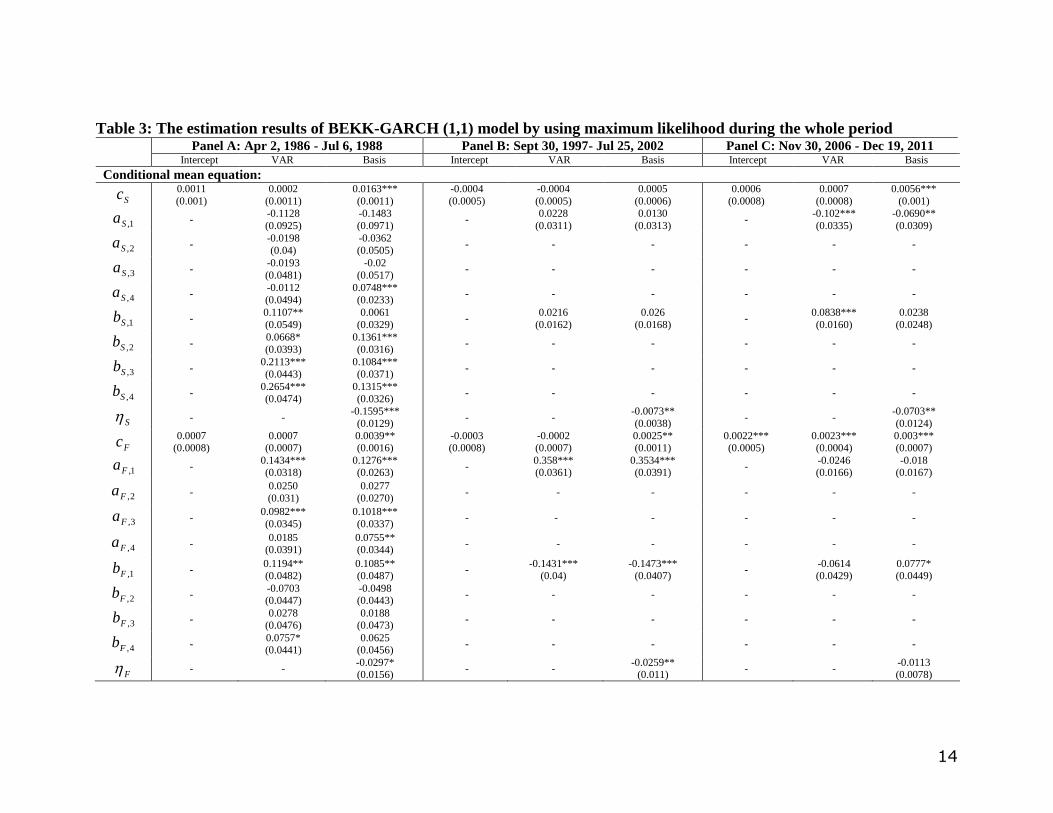
Notes: 1. (a) Intercept-BEKK-GARCH models are estimated by equations (1), (2), and (7). (b) Vector autoregressive (VAR)-BEKK-GARCH models are estimated by equations

(3), (4) and (7). (c) Basis-BEKK-GARCH models are estimated by equations (5), (6) and (9). 2. *, ** and *** indicate the statistical significance at the 10%, 5% and 1% levels

respectively. 3. Numbers in parentheses are the standard errors. 4. L is the value of the log-likelihood function calculated by equation (10). 5. Q and 2Q are the Ljung–Box

statistics of standardized residuals and standardized squared residuals.

16

Table 4: The estimation results of CCC-GARCH (1,1) model by using maximum likelihood during whole period

Panel A: Apr 2, 1986 - Jul 6, 1988 Panel B: Sept 30, 1997- Jul 25, 2002 Panel C: Nov 30, 2006 - Dec 19, 2011 Intercept VAR Basis Intercept VAR Basis Intercept VAR Basis

Conditional mean equation:

Sc 0.0010

(0.0013)

0.0006

(0.0011)

0.0133***

(0.0008)

-0.0003

(0.0004)

-0.0003

(0.0005)

0.0006

(0.0006)

0.0009

(0.0008)

0.0009

(0.0008)

0.0063***

(0.0009)

1,Sa - -0.0547

(0.0348)

-0.0604***

(0.0036) -

0.0261

(0.0314)

0.0151

(0.0322) -

-0.140***

(0.0426)

-0.0851**

(0.0396)

2,Sa - -0.0464

(0.0441)

-0.053***

(0.0207) - - - - - -

3,Sa - -0.0271

(0.0570)

-0.0065

(0.0242) - - - - - -

4,Sa - -0.0318

(0.0529)

0.0973***

(0.0101) - - - - - -

1,Sb - 0.0982*

(0.0529)

-0.0224

(0.0200) -

0.0177

(0.0168)

0.0279

(0.0219) -

0.1268***

(0.0187)

0.0345

(0.0278)

2,Sb

- 0.0846**

(0.0360)

0.1005***

(0.0184) - - - - - -

3,Sb - 0.2187***

(0.0408)

0.1149***

(0.0211) - - - - - -

4,Sb - 0.245***

(0.0455)

0.1307***

(0.0209) - - - - - -

S - - -0.131***

(0.0077) - -

-0.0071**

(0.0035) - -

-0.0741***

(0.0112)

Fc 0.0007

(0.0008) 0.0007

(0.0007) 0.0022

(0.0018) 5.16E-05 (0.001)

-0.0001 (0.0008)

0.002* (0.0011)

0.0024*** (0.0005)

0.0025 (0.0005)

0.0033*** (0.0007)

1,Fa - 0.16092***

(0.0407)

0.1437***

(0.0296) -

0.3582***

(0.0355)

0.3131***

(0.0365) -

-0.0223

(0.0183)

-0.0116

(0.0175)

2,Fa - 0.0289

(0.0309)

0.0341

(0.0358) - - - - - -

3,Fa - 0.0949**

(0.0371)

0.1046***

(0.0324) - - - - - -

4,Fa - 0.0354

(0.0399)

0.0535

(0.0403) - - - - - -

1,Fb - 0.1126 ** (0.0487)

0.1008* (0.0542)

- -0.129*** (0.0421)

-0.0493** (0.0218)

- -0.0422 (0.0431)

-0.0665 (0.0453)

2,Fb - -0.0678

(0.0456)

-0.0602

(0.0472) - - - - - -

3,Fb - 0.0191

(0.0472)

0.0105

(0.0504) - - - - - -

4,Fb - 0.0656

(0.0439)

0.0567

(0.0453) - - - - - -

F - - -0.015

(0.017) - -

-0.0162*

(0.0092) - -

-0.0146*

(0.0077)

17

Table 4: (Continued)

Panel A: Apr 2, 1986 - Jul 6, 1988 Panel B: Sept 30, 1997- Jul 25, 2002 Panel C: Nov 30, 2006 - Dec 19, 2011 Intercept VAR Basis Intercept VAR Basis Intercept VAR Basis

Conditional variance-covariance equation:

SS 0.0003 ***

(1.10E-05)

0.0002 *

(0.0001)

7.47E-05***

(1.14E-05)

9.2E-06***

(2.36E-06)

9.11E-10***

(2.33E-06)

9.91E-06***

(2.53E-06)

0.0002***

(2.46E-05)

0.0002***

(2.8E-05)

0.0004***

(1.82E-05)

FF 1.65E-05**

(2.3289)

1.72E-05**

(8.23E-06)

1.89E-05**

(9.63E-06)

0.0004

(0.0003)

0.0003*

(0.0002)

1.25E-05

(3.58E-06)

8.2E-05***

(1.21E-05)

8.2E-05***

(1.19E-05)

0.0001***

(1.63E-05)

SS -0.02***

(0.0005)

-0.0137

(0.0157)

1.4911***

(0.0304)

0.1198***

(0.0163)

0.1135***

(0.0154)

0.1159***

(0.0158)

0.0573***

(0.0104)

0.0613***

(0.0136)

0.101***

(0.0216)

FF 0.15*** (0.0369)

0.161*** (0.041)

0.1698*** (0.0437)

-0.007*** (0.0001)

0.0169 (0.0116)

-0.0038*** (0.0003)

0.6499*** (0.0332)

0.6327*** (0.0466)

0.6908*** (0.0395)

SS 0.58***

(0.0131)

0.4984*

(0.2767)

-0.004***

(0.0012)

0.8584***

(0.0178)

0.8642***

(0.0170)

0.8607***

(0.0176)

0.6322***

(0.04)

0.6501***

(0.0366)

-0.0132

(0.0373)

FF 0.81***

(0.0411)

0.801***

(0.0505)

0.7887***

(0.0524)

0.5204

(0.4224)

0.3978

(0.3306)

0.9811***

(0.0063)

0.4208***

(0.0294)

0.4213***

(0.0296)

0.2617***

(0.0403)

SS - - 0.0062*** (0.0008)

- - -1.34E-05 (1.97E-05)

- - 0.0147*** (0.0011)

FF - - -2.40E-05

(0.0004) - -

2.51E-05***

(6.49E-06) - -

0.0029***

(0.001)

Conditional correlation equation:

0.103** (0.0439)

0.118 *** (0.0441)

0.1260** (0.0492)

0.2982*** (0.0299)

0.3480*** (0.026)

0.3444*** (0.0267)

0.0554* (0.0301)

0.0621** (0.0316)

0.0696** (0.0315)

L 2687.813 2741.790 2837.206 5827.343 5880.906 5900.151 5767.511 5776.375 5941.987

Test for higher order ARCH effect

Spot equations 15Q 24.064* 18.205 60.143*** 27.295** 21.650 15.922 22.116 15.744 15.473

152Q 26.183*** 22.914* 40.009*** 20.195 20.754 21.448 17.750 14.262 5.9678

Futures equations

15Q 43.758*** 11.073 11.982 13.2 11.458 15.837 18.966 21.788 18.462

152Q 12.848 18.961 19.560 1.2405 0.9177 2.2377 0.8527 0.9040 0.9922

Notes: 1. (a) Intercept-CCC-GARCH models are estimated by equations (1), (2) and (8). (b) Vector autoregressive (VAR)-CCC-GARCH models are estimated by equations (3),

(4) and (8). (c) Basis-CCC-GARCH models are estimated by equations (5), (6) and (9). 2. *, ** and *** indicate the statistical significance at the 10%, 5% and 1% levels

respectively. 3. Numbers in parentheses are the standard errors. 4. L is the value of the log-likelihood function calculated by equation (10). 5. Q and 2Q are the Ljung–Box

statistics of standardized residuals and standardized squared residuals.

18

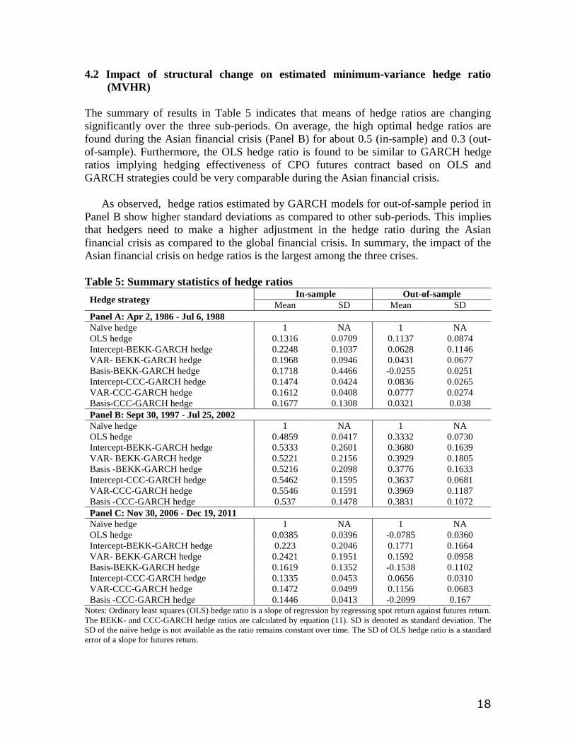
4.2 Impact of structural change on estimated minimum-variance hedge ratio

(MVHR)

The summary of results in Table 5 indicates that means of hedge ratios are changing

significantly over the three sub-periods. On average, the high optimal hedge ratios are

found during the Asian financial crisis (Panel B) for about 0.5 (in-sample) and 0.3 (out-

of-sample). Furthermore, the OLS hedge ratio is found to be similar to GARCH hedge

ratios implying hedging effectiveness of CPO futures contract based on OLS and

GARCH strategies could be very comparable during the Asian financial crisis.

As observed, hedge ratios estimated by GARCH models for out-of-sample period in

Panel B show higher standard deviations as compared to other sub-periods. This implies

that hedgers need to make a higher adjustment in the hedge ratio during the Asian

financial crisis as compared to the global financial crisis. In summary, the impact of the

Asian financial crisis on hedge ratios is the largest among the three crises.

Table 5: Summary statistics of hedge ratios

Hedge strategy In-sample Out-of-sample

Mean SD Mean SD

Panel A: Apr 2, 1986 - Jul 6, 1988

Naïve hedge 1 NA 1 NA OLS hedge 0.1316 0.0709 0.1137 0.0874 Intercept-BEKK-GARCH hedge 0.2248 0.1037 0.0628 0.1146

VAR- BEKK-GARCH hedge 0.1968 0.0946 0.0431 0.0677 Basis-BEKK-GARCH hedge 0.1718 0.4466 -0.0255 0.0251 Intercept-CCC-GARCH hedge 0.1474 0.0424 0.0836 0.0265 VAR-CCC-GARCH hedge 0.1612 0.0408 0.0777 0.0274 Basis-CCC-GARCH hedge 0.1677 0.1308 0.0321 0.038 Panel B: Sept 30, 1997 - Jul 25, 2002

Naïve hedge 1 NA 1 NA OLS hedge 0.4859 0.0417 0.3332 0.0730 Intercept-BEKK-GARCH hedge 0.5333 0.2601 0.3680 0.1639 VAR- BEKK-GARCH hedge 0.5221 0.2156 0.3929 0.1805 Basis -BEKK-GARCH hedge 0.5216 0.2098 0.3776 0.1633 Intercept-CCC-GARCH hedge 0.5462 0.1595 0.3637 0.0681 VAR-CCC-GARCH hedge 0.5546 0.1591 0.3969 0.1187 Basis -CCC-GARCH hedge 0.537 0.1478 0.3831 0.1072 Panel C: Nov 30, 2006 - Dec 19, 2011

Naïve hedge 1 NA 1 NA OLS hedge 0.0385 0.0396 -0.0785 0.0360 Intercept-BEKK-GARCH hedge 0.223 0.2046 0.1771 0.1664 VAR- BEKK-GARCH hedge 0.2421 0.1951 0.1592 0.0958 Basis-BEKK-GARCH hedge 0.1619 0.1352 -0.1538 0.1102 Intercept-CCC-GARCH hedge 0.1335 0.0453 0.0656 0.0310 VAR-CCC-GARCH hedge 0.1472 0.0499 0.1156 0.0683 Basis -CCC-GARCH hedge 0.1446 0.0413 -0.2099 0.167

Notes: Ordinary least squares (OLS) hedge ratio is a slope of regression by regressing spot return against futures return.

The BEKK- and CCC-GARCH hedge ratios are calculated by equation (11). SD is denoted as standard deviation. The

SD of the naïve hedge is not available as the ratio remains constant over time. The SD of OLS hedge ratio is a standard

error of a slope for futures return.

19

4.3 Impact of structural change on hedging effectiveness

Table 6 reports the variance of portfolio and variance reduction for unhedged and hedged

returns produced by naïve, minimum variance-OLS and various GARCH hedging

models.

Table 6: Hedging effectiveness of Malaysian CPO futures

Hedge strategy

In-sample Out-of-sample

Variance of

portfolio

Variance

reduction (%)

Variance of

portfolio

Variance

reduction (%)

Panel A: Apr 2, 1986 - Jul 6, 1988 Unhedged CPO portfolio 0.000819 - 0.000627 -

Hedged CPO portfolio:

Naïve hedge 0.0010908 -33.19068 0.001211 -93.1138

OLS hedge 0.0008126 0.78056 0.000617 1.558

Intercept-BEKK-GARCH hedge 0.0005952 27.3264 0.000618 1.53

VAR-BEKK-GARCH hedge 0.0004022 50.8849 0.000545 13.044

Basis -BEKK-GARCH hedge 0.000621 24.132 0.001863 -197.079

Intercept-CCC-GARCH hedge 0.0007065 13.7282 0.00063 -0.4026

VAR-CCC-GARCH hedge 0.000409 50.114 0.000554 11.624

Basis-CCC-GARCH hedge 0.0007 14.513 0.001806 -187.9868

Panel B: Sept 30, 1997 - Jul 25, 2002 Unhedged CPO portfolio 0.000653 - 0.00056 -

Hedged CPO portfolio:

Naïve hedge 0.000663 -1.0504 0.000698 -24.553

OLS hedge 0.000571 12.612 0.000514 8.176

Intercept-BEKK-GARCH hedge 0.000545 16.504 0.000495 11.622

VAR-BEKK-GARCH hedge 0.000554 15.216 0.000339 39.506

Basis -BEKK-GARCH hedge 0.000564 13.574 0.000316 43.655

Intercept-CCC-GARCH hedge 0.000764 17.0479 0.000512 8.554

VAR-CCC-GARCH hedge 0.00055 15.798 0.000384 31.38

Basis-CCC-GARCH hedge 0.000539 17.476 0.000307 45.146

Panel C: Nov 30, 2006 - Dec 19, 2011 Unhedged CPO portfolio 0.000781 - 0.000509 -

Hedged CPO portfolio:

Naïve hedge 0.001245 -59.3563 0.002317 -355.1356

OLS hedge 0.000781 0.095 0.000499 1.892

Intercept-BEKK-GARCH hedge 0.000737 5.682 0.0005 1.837

VAR-BEKK-GARCH hedge 0.000719 7.962 0.000489 3.882

Basis-BEKK-GARCH hedge 0.000681 12.789 0.000421 17.275

Intercept-CCC-GARCH hedge 0.000769 1.531 0.000543 -6.6563

VAR-CCC-GARCH hedge 0.000745 4.617 0.000458 10.075

Basis-CCC-GARCH hedge 0.000719 7.959 0.000539 -5.8768 Notes: 1. The variance of unhedged CPO portfolio is generated from the variance of CPO spot return. 2. The variance

of hedged CPO portfolio is computed by equation (12). 3. The risk reduction is calculated by equation (13).

As observed in Table 6, it shows that naïve strategy is the worst strategy as it

increases the risk of hedged portfolio. The VAR-BEKK-GARCH model is found as the

superior model in Panel A as it reduces 50.88 per cent of the risk (in-sample) and 13.04

per cent of the risk (out-of-sample). In Panel B, besides having relatively high dynamic

hedge ratios within the range of 0.48-0.56 (in-sample) and 0.33-0.40 (out-of-sample) as

20

shown in Table 5, an assumption of CCC-GARCH model with the basis term offers the

most effective risk reduction of 17.48 and 45.15 per cent for the in- and out-of-sample

respectively. In Panel C, a basis-BEKK-GARCH model achieves the highest risk

reduction of over 12-17 per cent for both in- and out-of-sample. Overall, it is clear that

the hedging strategies with the basis term generally outperform in reducing the risk of

CPO portfolio in Panel B and Panel C.

As compared between Panel B and Panel C, the marginal differences among models

suggest that the CPO futures hedging strategies underperform across the Asian and global

financial crises for both in- and out-of-sample respectively. As investors more concern

about future performance, the out-of-sample shows risk reduction of the superior model

declines sharply from 45.15 to 12.28 per cent. The low level of hedging effectiveness is

observed when futures return exhibits high volatility and fat-tailed distribution over the

period of 2006-2011. Overall, the result indicates that the linkage between spot and

futures prices in the long run (basis) is important to fit the extreme volatility during the

global financial crisis. In contrast, including a basis effect into the GARCH model cannot

sustain its high performance in reducing the risk during the global financial crisis as

compared to previous crisis.

5. Conclusions

This study extends Zainudin and Shaharudin (2011) on Malaysian crude palm oil (CPO)

futures market by examining the hedging effectiveness based on the minimum-variance

hedge ratios from eight model specifications. These models were evaluated during the

three financial crises namely, the world economic recession in 1986, Asian financial

crisis in 1997/1998 and global financial crisis in 2008/2009 respectively. Subsequently,

in-and out-of sample of the minimum variance of hedge ratio is compared during each

sub-period. As the in- and out-of-sample analysis provides same finding, this study

focuses on the out-of-sample forecasting evaluation results.

Notable findings are: First, it is evidently clear that GARCH models with basis term

outperform others during the Asian financial crisis (AFC) and global financial crisis

(GFC) respectively. Second, during the Asian financial crisis, the high dynamic hedge

ratios contribute to the superiority of CCC-GARCH model with risk reduction of 45.15

per cent. The declining hedge ratio in GFC leads to the emergence of BEKK-GARCH

model which provides the most risk reduction of 17.26 per cent. Third, from AFC to

GFC, the risk reduction of hedging strategy declines sharply from 45.15 to 17.28 per

cent. Two possible reasons are; Firstly, unlike AFC, the epicenter of GFC was in the

United States and subsequently extended to Europe. Secondly, episode of bad news was

released to the market one after another in prolonged period, which caused

ineffectiveness of hedging strategy as shocks were largely unanticipated.

Overall, this study concludes: First, the high dynamic hedge ratio during the Asian

financial crisis implies that CPO market participants are sensitive to CPO spot and

futures movement. Second, the superior GARCH model with the basis term cannot

21

sustain its performance in terms of risk reduction during the crisis period. This shows that

the Malaysian CPO futures market provides a low level of hedging effectiveness during

the global financial crisis, which is mainly caused by excess kurtosis in the markets. This

finding is found to be inconsistent with Ong et al (2012) who find that stable movement

of CPO spot price in 2009-2010 contributes to the low level of hedging effectiveness.

The policy implication is clear. Although the effectiveness of Malaysian CPO futures

is low during the recent crisis, the minimum-variance hedge ratio analysis has managed

to compare the performance of various hedging models. By understanding the

effectiveness of various hedging models, the CPO market participants can switch

between the models in different volatility periods to cover their risk exposure in the spot

market.

References

Ahmed S. (2007) Effectiveness of time-varying hedge ratio with constant conditional

correlation: an empirical evidence from the US treasury market. ICFAI Journal of

Derivatives Markets 4(2): 22-30.

Alizadeh, A.H., Kavussanos, M.G. and Menachof, D.A. (2004) Hedging against bunker

price fluctuations using petroleum futures contracts: constant versus time-varying hedge

ratios. Applied Economics 36 (12): 1337-1353.

Anderson, R.W. and Danthine, J.P. (1981) Cross hedging. The Journal of Political

Economy 89(6): 1182-1196.

Baillie, R.T. and Myers, R.J. (1991) Bivariate GARCH estimation of the optimal

commodity futures hedge. Journal of Applied Econometrics 6(2): 109-124.

Bollerslev, T. (1990) Modelling the coherence in short-run nominal exchange rates: a

multivariate generalized ARCH model. Review of Economics and Statistics 72(3): 498-

505.

Bollerslev, T., Engle, R.F. and Wooldridge, J.M. (1988) A capital asset pricing model

with time-varying covariances. Journal of Political Economy 96(1): 116-131.

Brooks, C., Henry, O.T. and Persand, G. (2002) The effect of asymmetries on optimal

hedge ratio. The Journal of Business 75(2): 333-352.

Central Bank Malaysia (2009) Monthly Statistical Bulletin July 2009. Kuala Lumpur:

Central Bank.

Choudhry, T. (2002) Short-run deviations and optimal hedge ratio: evidence from stock

futures. Journal of Multinational Financial Management 13(2): 171-192.

22

Choudhry, T. (2004) The hedging effectiveness of constant and time-varying hedge ratios

using three Pacific Basin stock futures. International Review of Economics and Finance

13(4): 371-385.

Ederington, L.H. (1979) The hedging performance of the new futures market. Journal of

Finance 34(1): 157-170.

Engle, R.F. and Kroner, K.F. (1995) Multivariate simultaneous generalized ARCH.

Econometric Theory 11(1): 122-150.

Fama, E.F. (1984) Forward and spot exchange rates. Journal of Monetary Economics

14(3): 319–338.

Floros, C. and Vougas, D.V. (2004) Hedge ratios in Greek stock index futures market.

Applied Financial Economics 14(15): 1125-1136.

Giannopoulos, K. (1995) Estimating the time varying components of international stock

markets' risk. The European Journal of Finance 1(2): 129-164.

Howard, C.T. and D’Antonio, L.J. (1984) A risk-return measure of hedging effectiveness.

Journal of Financial and Quantitative Analysis 19(1): 101-112.

Hill, J. and Schneeweis, T. (1981) A note on the hedging effectiveness of foreign

currency futures. Journal of Futures Markets 1(4): 659-664.

Johnson, L.L. (1960) The theory of hedging and speculation in commodity futures. The

Review of Economic Studies 27(3): 139-151.

Kroner, K.F. and Sultan, J. (1993) Time varying distribution and dynamic hedging with

foreign currency futures. Journal of Financial and Quantitative Analysis 28(4): 535-551.

Kogan, L., Livdan, D. and Yaron, A. (2003) Futures prices in a production economy with

investment constraints. Working Paper, MIT.

Lien, D., Tse, Y.K. and Tsui, A.K.C. (2002) Evaluating the hedging performance of the

constant-correlation GARCH model. Applied Financial Economics 12(11): 791-798.

Lien, D. and Yang, L. (2008) Hedging with Chinese metal futures. Global Finance

Journal 19(2): 123-138.

Malaysian Palm Oil Board. Available from http://www.mpob.gov.my/. Accessed 24

October 2012.

Moschini, G.C. and Myers, R.J. (2002) Testing for constant hedge ratios in commodity

markets: a multivariate GARCH approach. Journal of Empirical Finance 9(5): 589-603.

23

Ng, V.K. and Pirrong, S.C. (1994) Fundamentals and volatility: storage, spreads, and the

dynamics of metals prices. Journal of Business 67(2):203-230.

Ong, T.S., Tan, W.F. and Teh, B.H. (2012) Hedging effectiveness of crude palm oil

futures market in Malaysia. World Applied Sciences Journal 19(4): 556-565.

Park, T.H. and Switzer, L.N. (1995) Time-varying distribution and the optimal hedge

ratios for stock index futures. Applied Financial Economics 5(3): 131-137.

Stein, J.L. (1961) The simultaneous determination of spot and futures prices. The

American Economic Review 51(5): 1012-1025.

Switzer, L.N. and El-Khoury, M. (2007) Extreme volatility, speculative efficiency, and

the hedging effectiveness of the oil futures markets. Journal of Futures Markets 27(1):

61-84.

Tong, W.H.S. (1996) An examination of dynamic hedging. Journal of International

Money and Finance 15(1): 19-35.

United Nations Development Program (UNDP)(2009) The Global Financial Crisis and

the Malaysian Economy: Impact and Response. A Joint Report by the Institute of

Strategic and International Studies (ISIS) and the Faculty of Economics and

Administration (UNDP Malaysia).

Working, H. (1953) Futures trading and hedging. The American Economic Review 43(3):

314-343.

Wu, F., Guan, Z. and Myers, R.J. (2011) Volatility spillover effects and cross hedging in

corn and crude oil futures. Journal of Futures Markets 31(11): 1052-1075.

Zainudin, R. and Shaharudin, R.S. (2011) Multi mean GARCH approach to evaluating

hedging performance in the crude palm oil futures market. Asian Academy of

Management Journal of Accounting and Finance 7(1): 111-130.