Abstract: Greenhouse gas (GHG) emissions from the global shipping sector have been increasingdue to global economic growth. The International Maritime Organization (IMO) has set a goal ofhalving GHG emissions from the global shipping sector by 2050 as compared with 2008 levels, andhas responded by introducing several international regulations to reduce the GHG emissions ofmaritime transportation. The impact of GHG emissions’ regulation and measures to curb them havebeen evaluated in the IMO’s GHG studies. However, the long-term influence of these GHG emissionmeasures has not yet been assessed. Additionally, the impact of various GHG reduction measureson the shipping and shipbuilding markets has not been considered; accordingly, there is room forimprovement in the estimation of GHG emissions. Therefore, in this study, a model to consider GHGemission scenarios for the maritime transportation sector was developed using system dynamics andwas integrated into a shipping and shipbuilding market model. The developed model was validatedbased on actual results and estimation results taken from a previous study. Subsequently, simulationswere conducted, allowing us to evaluate the impact and effectiveness of GHG emission-curbingmeasures using the proposed model. Concretely, we conducted an evaluation of the effects of currentand future measures, especially ship speed reduction, transition to liquid natural gas (LNG) fuel,promotion of energy efficiency design index (EEDI) regulation, and introduction of zero-emissionships, for GHG emission reduction. Additionally, we conducted an evaluation of the combination ofcurrent and future measures. The results showed that it is difficult to achieve the IMO goals for 2050by combining only current measures and that the introduction of zero-emission ships is necessaryto achieve the goals. Moreover, the limits of ship speed reduction were discussed quantitatively inrelation to the maritime market aspect, and it was found that the feasible limit of ship speed reductionfrom a maritime market perspective was approximately 50%.
Keywords: GHG emission measures; international shipping; system dynamics; scenario planning;deceleration operation; energy efficiency design index; LNG fuel; zero-emission ships
1. Introduction1.1. Background and Research Objective
Sea cargo movement continues to rise because of global economic growth. As a result,there has been an increase in the number of ships used in maritime transportation, whichhas led to corresponding growth in greenhouse gas (GHG) emissions. The InternationalMaritime Organization (IMO) has estimated GHG emissions by the maritime transportationsector in recent years [1] and has established regulations for GHG emissions based onthat estimation.
To project GHG emissions by the maritime transportation sector in the future, it isimperative to forecast fleet volumes. For this purpose, accurate demand forecasting forshipping and shipbuilding is important. However, as the shipping and shipbuilding market
is a complex integrated system, the development of an accurate demand forecasting modelis not easy. For example, sea cargo movement is, fundamentally, complexly influenced bythe world economy. Orders for newly built ships are also influenced by various factors,such as the price of the ship, the order books of shipyards, and the demolition of olderships. In addition, when shipyards receive orders from shipping companies, the orderbooks and the ship price change concurrently. Fleet volumes fluctuate with the number ofships under construction and with ship demolition.
Thus, demand forecasting for shipping and shipbuilding is essential to estimate futureGHG emissions. However, the complex and dynamic relationship between shipping andshipbuilding markets was not considered in the IMO’s GHG study. Therefore, there is roomfor improvement in the estimation of GHG emissions. Additionally, research evaluatingthe long-term impact of GHG emission measures is insufficient.
With these points in mind, this study develops a model to evaluate GHG emissionmeasures for the maritime transportation sector using system dynamics. Using the pro-posed model, simulations were conducted, based on which we evaluated the impact andeffectiveness of current and future measures for GHG emission reduction. Then, we built atheoretical framework to develop a model that comprehensively evaluates the impact ofGHG emission measures in the maritime market.
1.2. Related Literature
Some studies have already been conducted to evaluate the social and economicimpacts of GHG emission regulations. Komiyama et al. [2] predicted changes in long-termenergy demand and power supply composition under the constraint of carbon dioxide(CO2) emission in Japan. Holz et al. [3] predicted changes in global CO2 emissions andsurface temperatures using system dynamics models and analyzed carbon dioxide removaldeployment scenarios.
Similarly, to support decision-making to solve the complex problem of GHG emissionsin the maritime transportation sector, some studies have forecasted GHG emissions anddiscussed effective measures to curb emissions in the maritime logistics field. In the thirdIMO GHG study [1], current CO2 emissions were estimated using automatic identificationsystem (AIS) data, while future CO2 emissions were forecasted using the representativeconcentration pathway and shared socioeconomic pathway scenarios. In addition to thesescenarios, a fuel mix scenario in which liquid natural gas (LNG) is introduced with themain fuel as well as a fuel efficiency improvement scenario were inputted to forecast CO2emissions. In the fourth IMO GHG study [4], CO2 emissions estimations and future CO2emissions were updated; additionally, estimation of carbon intensity and an analysis ofthe relations between CO2 reduction costs and CO2 abatement potential for each GHGreduction technology were conducted. Similarly, Faber et al. [5] estimated current CO2emissions and considered the impact of an emissions trading scheme on the maritimetransportation sector. Lindstad et al. [6] estimated and compared the well-to-wake GHGemissions of LNG fuel and traditional fuels (i.e., marine gasoil (MGO) and heavy fuel oil(HFO)). The results indicated that increased use of LNG engines would increase GHGemissions compared with conventional fuels (MGO, HFO, and Scrubber, as well as verylow sulfur fuel oil) by increasing methane emissions. Rehmatulla et al. [7] quantifiedthe implementation of over 30 energy-efficient and CO2 emission technologies in theshipping sector using a cross-sectional survey. These studies focused on the estimationand forecasting of GHG emissions and carbon intensity, as well as the evaluation ofGHG emission measures. However, deployment scenarios for GHG emission reductiontechnologies were not provided, and comprehensive scenarios to achieve IMO goals (i.e.,how GHG reduction measures should be combined and when the measures would start toapply) have not yet been presented.
As can be gleaned by the points highlighted above, estimates of GHG emissions in theshipping industry and the efficiency evaluation of GHG emission reduction technologieshave been conducted in previous studies [1,4–7]. However, these previous studies [1,4–7]
Sustainability 2021, 13, 2760 3 of 22
do not provide a quantitative assessment of the impact of GHG emission measures on theshipping and shipbuilding markets, nor do they fully discuss scenarios for introducingvarious GHG emission measures. In recent years, there has been a deceleration in shipoperations because of a slump in maritime market conditions and soaring fuel costs [8].Smith [9] analyzed the impact of ship speed reduction operations on GHG reductions andship owner’s profits and found that, ceteris paribus, operations to maximize a ship owner’sprofits negate the benefit of emissions reductions achieved through technology. However,it is difficult to grasp the time-series changes in the shipping and shipbuilding marketsthrough ship speed reduction, because various factors in the shipping and shipbuildingmarkets and their causal relationships were not considered. From the above, it appearsthat deceleration is also effective in reducing GHG emissions; however, the impact ofdeceleration on the shipping and shipbuilding market has not been fully considered.
On the other hand, in order to support decision making in the maritime industry,various studies on analyzing and modeling of maritime markets have been conducted.Nielsen [10] analyzed the maritime market using a causal loop diagram and developeda forecasting model for the shipbuilding market. Sakalayen et al. [11] formulated shipquantity order fluctuations using Newton’s law of gravitation and developed a predictionmodel for order quantity by applying the multivariate autoregressive integrated movingaverage model. Gourdon [12] analyzed the price and cost determinants of new shipsand discussed the impact of intervention by government agencies in the shipbuildingmarket. Shin and Lim [13] developed an empirical model of national competition in theshipbuilding industry using a Cournot oligopoly model based on the real behavior ofshipbuilding companies. Taylor [14], the Japan Maritime Research Institute SD StudyGroup [15], and Engelen et al. [16] developed forecasting models for the shipping andshipbuilding market using system dynamics. Similarly, in a previous study by the presentauthors [17], we developed a model to forecast the main elements of the shipbuildingmarket, such as the amount of sea cargo movement, order of ships, construction, andscrapping, using system dynamics. Using this model, we forecast fleet volume, which isthe key element in GHG emission estimation, by setting parameters such as GDP and cargotransportation distance. Although analysis and modeling in the maritime market havebeen carried out in these studies [10–17], a model that considers both the maritime marketand GHG emissions has not yet been developed.
Against these backgrounds, in this study, a GHG emission prediction model is devel-oped and integrated into a model that forecasts the demand for shipbuilding in a previousstudy [17]. Based on the aforementioned considerations, the characteristics of this studycan be summarized as follows:
• The long-term impact of current GHG reduction measures, such as the deceleration ofoperations of ships, transition to LNG fuel, and promotion of the energy efficiencydesign index (EEDI), is evaluated.
• GHG emission reduction countermeasures based on the introduction of zero-emissionships, which are being considered for introduction in the future, are considered.
• The GHG emission reduction effect by current measures and future measures alone isclarified using the proposed model. Additionally, the impact and effectiveness of com-bining current measures and future measures are evaluated using the proposed model.
• The limitations of operating speed deceleration measures on shipping and the ship-building market are evaluated quantitatively using the proposed model.
2. Basic Concept2.1. Overview of System Dynamics
System dynamics (SD), which was developed at the Massachusetts Institute of Tech-nology in 1956, is a well-known numerical simulation technique used to analyze complexand dynamic systems [18]. The fundamental concept of system dynamics is modelingcausal relations by mathematically considering time delays between the elements of thesystem and conducting a simulation using the developed model. Using this technique, we
Sustainability 2021, 13, 2760 4 of 22
can analyze complex systems based on logical reasoning, which helps ascertain the charac-teristics and dynamic behaviors of the systems. In recent years, SD has been progressing,mainly owing to the work of Sterman [19] and colleagues; Sterman et al. [20] developed apolicy decision-making model for global GHG emission reductions.
This study uses SD to develop a model that considers the relationship between theshipping and shipbuilding markets and GHG emissions in the shipping sector. On thisbasis, deployment scenarios for GHG reduction measures are examined.
2.2. Basic Configuration of the SD Model
The target ship type in this study is the bulk carrier. The target cargo commoditiesinclude iron ore, coal, and grain. The basic concept of demand forecasting as employed inthis study is shown in Figure 1. This figure was described based on the concept of stockand flow diagram [19] in SD. “Flow” shows the inflow and outflow of substances (i.e.,ships and GHG in this figure) into the element. “Information Flow” shows the causalrelationship between elements and shows that an element affects direction of the arrow inrelation to another element. “Information Flow Considering Time Delay” indicates that anelement affects the element in the direction of the arrow with a time delay. As shown in thefigure, the SD model in this study consists of the following six sub-models:
1. Cargo transportation prediction model: This model forecasts the total volume of seacargo movement based on world gross domestic product (GDP) and cargo transporta-tion distance.
2. Order prediction model: This model forecasts the number of orders based on seacargo movement, fleet volume, backlog of shipyard, and ship price. It considers thechange in the number of newly built ships due to ship operating speed reduction.
3. Construction model: Ship construction period is influenced by construction capacityand shipyard order book. The model estimates the total number of ships constructed.
4. Ship price prediction model: This model forecasts the price of a newly built shipbased on the backlog of shipyards.
5. Scrap model: This model predicts the number of scrapped ships each month based onthe ship’s age and shipping market condition. It considers the change in the amountof scrapped ships due to ship operating speed reduction.
6. GHG emissions prediction model: This model forecasts GHG emissions based onthe number of ships and fuel consumption. It considers differences in engine perfor-mance by ship’s age and size. Fuel consumption of auxiliary engine and boiler anddifferences in fuel type are also considered.
The relationships between sub-models are as follows:
• The total volume of sea cargo movement is calculated by inputting world GDP andcargo transportation distance using (1) the cargo transportation prediction model.
• The ship running distance, which is a measure of transportation efficiency of shipping,is calculated based on sea cargo movement and fleet volume. After that, ship ordersand scrapped ships are calculated using (2) the order prediction model and (5) thescrap model.
• The number of orders is determined, the orders for new ships are added to the orderbooks in shipyards, and the amount of ship construction and ship price are calculatedconsidering shipyard condition using (3) the construction model and (4) the ship priceprediction model.
• In (6) the GHG emissions prediction model, the fuel consumption for each ship isestimated considering operating speed, ship performance, ship composition, andtechnological developments for GHG reduction. GHG emissions are calculated basedon fuel consumption and fleet volume. Moreover, the operating speed influences thetransport efficiency of each ship, and hence also the ship running distance. Shippingand shipbuilding market conditions are changed by this influence.
• Fleet volume and ship composition are updated based on the amounts of ship con-struction and scrap.
Sustainability 2021, 13, 2760 5 of 22
Figure 1. Evaluation model for greenhouse gas (GHG) reduction measures. GDP, gross domestic product.
In summary, this SD model considers the mutual relationships between each of threefacets: ship operation, shipping, and shipbuilding markets. Sub-models (1)–(4) wereused in previous studies (Wada et al. [17,21]), while (5) the scrap model was improvedby introducing the scrap rate to update the ship composition in this study. Additionally,(6) the GHG emissions prediction model is also newly developed.
3. GHG Emissions Prediction Model3.1. Overview of GHG Emissions Prediction Model
GHG emissions consist of gases such as CO2, methane (CH4), and nitrous oxide (N2O),of which CO2 accounts for a large proportion. The IMO GHG studies ([1,4]) focused on theestimation of CO2 emissions; we do the same, to allow for a comparison. Additionally, wefocused on CO2 emission from shipping based on IMO’s initial GHG emission reductionstrategy [22]. CO2 emissions from ship construction are not considered in this study.
The volume of CO2 emissions was determined by fleet volume and fuel consumption.Fleet volume is closely related to the development of shipping and shipbuilding markets,while various factors, such as the fuel efficiency of ships, ship operation, and fuel type, arerelated to fuel consumption. Therefore, it is important to define and model the relationshipamong these elements in CO2 emission estimation using the SD model. Based on the above,in estimating CO2 emissions, the following points were considered:
• Ship speed deceleration affects shipping and shipbuilding markets. Ship operat-ing speed deceleration influences on shipping and shipbuilding markets and GHGemissions reduction is considered in this study.
• The fuel efficiency performance of ships differs depending on the year of their con-struction, due to technological developments and regulation changes. The time-serieschange in fuel efficiency performance of ships is considered in this study.
The models, excluding the GHG emissions prediction model highlighted in Figure 1,were developed in previous studies [17,21]. By integrating the GHG emissions predictionmodel into the previous study’s model and modification of the scrap model, it is possible toevaluate the impact of GHG reduction measures and predict future CO2 emissions, whichis the purpose of this study. Additionally, the impact and effectiveness of operating speed
Sustainability 2021, 13, 2760 6 of 22
deceleration measures on shipping and shipbuilding markets were evaluated quantitativelyusing the proposed model.
3.2. Data Utilized in GHG Emissions Prediction Model Development
The data utilized for GHG emissions prediction model development are shown inTable 1. The details of each data type are explained below. The ship specification valuesare shown in Table 2. These values are used as representative ship types for each size. Thedefinition of each ship size is set as follows: Capesize: 100,000 deadweight tonnage (DWT)and over; Panamax: 65,000–99,999 DWT; Handymax: 40,000–64,999 DWT; and Handysize:10,000–39,999 DWT. This definition of ship classification follows that of Clarksons [23]:
(1) Ship composition: Ship composition shows the fleet volume for ships at all ages. Theship composition of Capesize, Panamax, Handymax, and Handysize from 2013 to2018 was obtained from Sea-web ships [24]. It should be noted that Sea-web ships is aships database provided by IHS Markit.
(2) Ship performance: Ship performance varies depending on the size of the ship. Theperformance items in this study are shown below.
(i) Main engine power: The main engine power is the value of the main enginemounted on the ship.
(ii) Service speed: The service speed is the average ship speed by a ship underloading condition and in calm weather.
(iii) Specific fuel consumption (SFC): SFC indicates fuel consumption per hour ofengine output. It depends on the ship’s size and age. The values for HFOships are sets based on the second IMO GHG study [25] and are summarizedin Table 3.
(iv) Fuel consumption of auxiliary equipment and boilers: Fuel consumption ofauxiliary equipment and boilers also impacts GHG emission. Fuel consump-tion by these ship elements is considered. The values are set based on thefourth IMO GHG study [4].
(3) Average voyage time: Average voyage time is determined by converting the annualaverage voyage days into monthly average hours.
(4) Average DWT: When calculating CO2 emissions, average DWT is required as arepresentative value for each ship size, as the unit of fleet volume is converted fromthe DWT to the number of ships. Average DWT was determined using the actualnumber of ships and the total DWT of the fleet volume.
(5) Calibration factor, CO2 emission correction coefficient: CO2 emissions estimationresults for each ship size have been reported in previous studies [4]. The calibrationfactor was introduced to reproduce the reported CO2 emissions, because ship sizeclassification and the representative value for each ship size are different betweenthis study and previous studies. This calibration factor was determined using theestimated CO2 values and actual ship composition data. Additionally, it is alsonecessary to consider ships whose size is below Handysize (less than 10,000 DWT)when calculating the CO2 emissions of a bulk carrier. Therefore, we introduced theCO2 emission correction coefficient to consider the CO2 emissions of smaller ships.The CO2 emission correction coefficient has an average value of 1.02, calculated fromthe actual value for ships smaller than and over 10,000 DWT.
(6) Scrap ship list: The scrap rate for each size is defined to update the ship composition,which is used when calculating CO2 emissions. The scrap ship list was used to definethe scrap rate.
Sustainability 2021, 13, 2760 7 of 22
Table 1. Data utilized to define greenhouse gas (GHG) emissions prediction model development. IMO, InternationalMaritime Organization; DWT, deadweight tonnage.
3.3. Model Development for GHG Emissions Prediction Model
CO2 emissions were calculated using Equations (1) and (2).
(1) Calculate main engine output by ship size using Equation (1). The difference inengine output depending on the ship’s size is considered; in addition, we considerthe effect of deceleration operating on the ratio of service speed to operating speed.Instantaneous main engine power (Pme) changes depending on the cube of the ratioof operating speed (Vt) to service speed (Vref ).
(2) Calculate monthly CO2 emissions using equation (2). First, fuel consumption is cal-culated by multiplying the main engine output calculated by SFC, which representsfuel consumption per hour of engine output, and voyage time. As shown in Table3, SFC is determined by the size and age of the ships. In addition, fuel consumptionof auxiliary equipment and boiler for each ship size is considered constant, as noted.For CO2 emissions below Handysize (0–9999 DWT), the effect is considered by multi-plying the total value of CO2 emissions for each size by the correction coefficient γ.It should be noted that the percentage of total CO2 emissions taken up by auxiliaryequipment and boiler is approximately 10.8% in the case that operating speed is 85.0%of service speed.
Pmeit = Pre f i ×
(Vti
tVre f i
)3
× αi, (1)
Sustainability 2021, 13, 2760 8 of 22
CO2t = ∑i
∑a
∑ε
{(Pmei
t × SFCia,ε,t × timei + Axi + Boi
)× C fε × Ni
a,ε,t
}× γ, (2)
where Pme is instantaneous main engine power (kW), Pref is main engine power(kW), Vref is service speed (knots), Vt is operating speed (knots), α is the calibrationfactor, CO2 is CO2 emission (g), SFC is fuel consumption per kWh (gfuel/kWh), Cfis carbon content in fuel (gCO2/gfuel), time is average voyage time (hours), N isthe number of ships (number), Ax is auxiliary equipment fuel consumption (g), Bois boiler fuel consumption (g), γ is the CO2 emission correction coefficient, i is shipsize (1: Capesize, 2: Panamax, 3: Handymax, 4: Handysize), a is the age of ships,ε is the fuel type (1: HFO, 2: LNG fuel, 3: zero-emission fuels), and t is simulationtime (months).
3.4. Correction of Order Prediction Model
In general, transport efficiency decreases as the ships slow down. By this logic, therequired fleet quantity per unit of cargo increases and, subsequently, the order quantityof ships increases. This study calculates ship running distance, which indicates transportefficiency using the sea cargo movement and fleet volume, and then uses this to calculatethe order and the scrap quantity. The ship running distance is calculated using Equation (3).
Et =VCtmt
Vt, (3)
where E is ship running distance (miles), VCtm is the sea cargo movement (tons × miles),V is the total fleet volume (DWT), and t is simulation time (months).
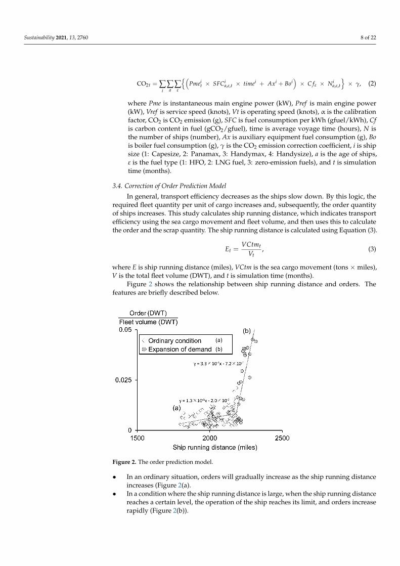
Figure 2 shows the relationship between ship running distance and orders. Thefeatures are briefly described below.
Figure 2. The order prediction model.
• In an ordinary situation, orders will gradually increase as the ship running distanceincreases (Figure 2(a).
• In a condition where the ship running distance is large, when the ship running distancereaches a certain level, the operation of the ship reaches its limit, and orders increaserapidly (Figure 2(b)).
Sustainability 2021, 13, 2760 9 of 22
The influence of operating speed reduction on the order prediction model is shown inFigure 3. Point A is the situation in Figure 2. In the case of Point B in Figure 3, operatingspeed was reduced by approximately 20%, and the order function moved in parallel by 20%to shorten the ship running distance. In the case of Point C in Figure 3, operating speed wasreduced by approximately 30%, and the order function moved in parallel by 30% to shortenthe ship running distance. Thus, the order prediction model moved gradually towardsthe critical juncture of shortening the ship running distance; as a result, the operation ofships was seen to reach the critical limit easily. The total number of orders, consideringthe influence of operating speed reduction, is calculated using Equation (4). It should benoted here that the basic concept of correction of orders was shown in a previous study byWada et al. [17]:
Ot = f1(Et, St) × Vt, (4)
where O is the total number of orders (DWT), f 1 is the order prediction model consideringoperating speed rate, E is the ship running distance (miles), S is the operating speed rate(-), V is the total fleet volume (DWT), and t is simulation time (months).
Figure 3. Relation between operating speed reduction scenario and order prediction model.
3.5. Update of Ship Composition
This study suggests that a ship’s age composition should reflect changes in shipperformance due to the year of construction. The calculation flow is as follows:
(1) Use the scrap model to calculate the amount of scrap. The scrap model was definedfor each size (Figure 4). An overview of the scrap model and the model developmentprocedures is given in a previous study (Wada et al. [17]). However, we modified thescrap model by considering the operating speed rate, using the same concept as inFigure 3.
(2) Use the scrap rate according to ship age to calculate the scrap ship by ship age. Thescrap rate was defined by normalizing the actual value of demolition (Figure 5). Thescrap ship list until 2018 was utilized to define the models. Ship composition wasupdated by deducting each age of scrap ships. After that, ship composition wasupdated for 1 month.
(3) Use the construction model to calculate the amount of constructed ships. The amountof constructed ships is added to 0 years of age for each size of ship composition.
Sustainability 2021, 13, 2760 10 of 22
Figure 4. Scrap model for each size of ship. (a) Scrap model for Capesize; (b) Scrap model for Panamax; (c) Scrap model forHandymax; (d) Scrap model for Handysize.
Figure 5. Scrap rate by ship age. (a) Scrap rate for Capesize; (b) Scrap rate for Panamax; (c) Scrap rate for Handymax;(d) Scrap rate for Handysize.
Sustainability 2021, 13, 2760 11 of 22
The scrap rate represents the probability of demolition for each age of ship based onthe actual scrap data. As shown in Figure 5, the average scrap age becomes younger asthe ship size increases. The average scrap age is 21.7 years for Capesize, 23.0 years forPanamax, 24.7 years for Handymax, and 27.3 years for Handysize. Using the scrap rate,we considered the actual conditions of scrap considering ship age. The ship composition iscalculated using Equations (5)–(8):
Dit = f i
2(Et, St) × Vit , (5)
Dia,t = f i
3
(Di
t
), (6)
Sdia,t = Sci
a,t − Dia,t, (7)
Scia,t+1 = Sdi
a+1,t + Ci0,t, (8)
where D is the amount of scrap (DWT), f 2 is each size of scrap model in Figure 4, E is shiprunning distance (miles), S is operating speed rate (-), V is fleet volume for each ship size(DWT), f 3 is the each scrap rate in Figure 5, Sd is ship composition deducted each age ofscrap ships (DWT), Sc is ship composition (DWT), C is the amount of construction (DWT),a is the age of ships, i is the size of ships, and t is simulation time (months).
4. Model Validation
To confirm the validity of the modeled predictions of CO2 emissions and ship com-position, hindcast simulations were performed for the 2013 to 2018 period. The purposeof this validation is to confirm the validity of the newly developed model (i.e., the GHGemission prediction model and update of ship composition) in this study. The validity ofthe number of orders, amounts of scrap, and the other elements of sub-models in Figure 1were confirmed in previous research [17,21]. The initial values are the input scenariosshown below.
(1) Fleet volume: 6.80 × 10⁸ (DWT)(2) Order books: 1.40 × 10⁸ (DWT)(3) Construction capacity: 9.85 × 10⁶ (DWT)(4) Ship amount under construction: 5.10 × 10⁷ (DWT).
The simulation results for CO2 emissions are shown in Table 4. From these results,CO2 emissions were estimated within an error margin of ±2.5%. There is no large error,and CO2 emissions can be predicted well.
Table 4. Simulation results of CO2 emissions from 2013 to 2018.
This Study(×106 tons) 176.6 181.7 182.3 189.0 193.4 196.8
Error (%) −0.6 +2.5 −1.0 −1.6 −2.5 +1.8
The simulation results for the ship composition are shown in Figure 6. The shipcomposition in December 2018 can be reproduced from the results. From these results, thevalidity of the entire model was confirmed.
Sustainability 2021, 13, 2760 12 of 22
Figure 6. Composition of observed and simulated ship ages in 2018.
In the fourth IMO GHG study [4], detailed ship movement data (i.e., AIS data) andvarious other data were utilized to estimate recent CO2 emissions. In this study, wedeveloped a model that obtained results similar to IMO’s GHG study without the use ofdetailed ship movement data. In the proposed model, CO2 emissions’ forecasting can beexecuted by setting the scenario for GDP and cargo transportation distance only. This is anadvantage for forecasting CO2 emissions under the proposed model.
5. Case Study
In this section, the influences of current and future GHG emission measure deploy-ment scenarios are considered using the proposed model. Concretely, evaluation of currentmeasures for GHG emission reduction, especially deceleration operation, transition to LNGfuel, and technological development to achieve EEDI regulation, is done in Section 5.1.In Section 5.2, we evaluate future measures for GHG emission reduction, especially theintroduction of zero-emission ships. In Section 5.3, we evaluate the combination of currentand future measures in GHG emission reduction. In Section 5.4, we consider the limitationof deceleration operation and the effectiveness of combining shipping and shipbuildingmarket models and GHG emission prediction models. In Section 5.5, we discuss thesimulation results from Sections 5.1–5.4.
5.1. Impact Assessment of Current Measures5.1.1. Overview of Current Measures
The current measures are explained in this section.
(1) Deceleration operation: This measure can suppress GHG emissions by reducing themain engine’s output to save fuel during voyages. The average operating speed forships has reduced since 2008.
(2) Transition to LNG fuel: LNG, which has the effect of reducing fuel consumptionand the carbon content rate, is drawing attention as an alternative to heavy fuel oil(HFO). The carbon content rate (Cf in Equation (2)) is 3.114 (gCO2/gfuel) in HFOand 2.750 (gCO2/gfuel) in LNG. SFC in Equation (2) is 156 g/kWh in LNG. In HFO,SFC in Equation (2) is utilized in Table 3. These values are from the fourth IMO GHGstudy [4]. Carbon content rate (Cf) and SFC were lower in LNG fuel than in HFO fuel.
(3) Technological development to achieve EEDI regulation: EEDI is the amount of CO2emissions when carrying 1 ton of cargo for 1 mile. By restricting this value, the fuel
Sustainability 2021, 13, 2760 13 of 22
efficiency of ships is promoted and CO2 emissions are reduced. As the percentage ofships in the fleet volume that has passed regulation value increases with each passingyear, it is necessary to take a long-term perspective on impact assessment of the EEDIregulation. In this study, we assumed that the EEDI regulation will be achieved bytechnology development, such as reduction of hull resistance and improvement ofpropeller efficiency in HFO ships.
5.1.2. Scenario Settings
To evaluate current GHG reduction measures, simulations for 2013–2050 were con-ducted. The market conditions in 2013 were used as initial values, and the followingscenarios for current measures were inputted:
(1) World GDP: Actual values for 2013–2019 were used and 3.5% GDP growth from 2020was assumed. This assumption was based on the average GDP growth rate from 1980to 2019, obtained from the International Monetary Fund [26].
(2) Cargo transportation distance: Actual values for 2013–2019 were used, and after 2020,the values were assumed to be constant.
(3) Operating speed reduction: It is still unclear how much ships will slow down in thefuture shipping industry. In this study, the actual value was used for 2013–2019, andafter 2020, it was assumed that the speed is linearly reduced until 2050, reaching theintensity of deceleration that achieves 40% deceleration in 2050. The influence ofoperating speed reduction on GHG emissions and the implication for the maritimemarket industry are discussed in Section 5.4.
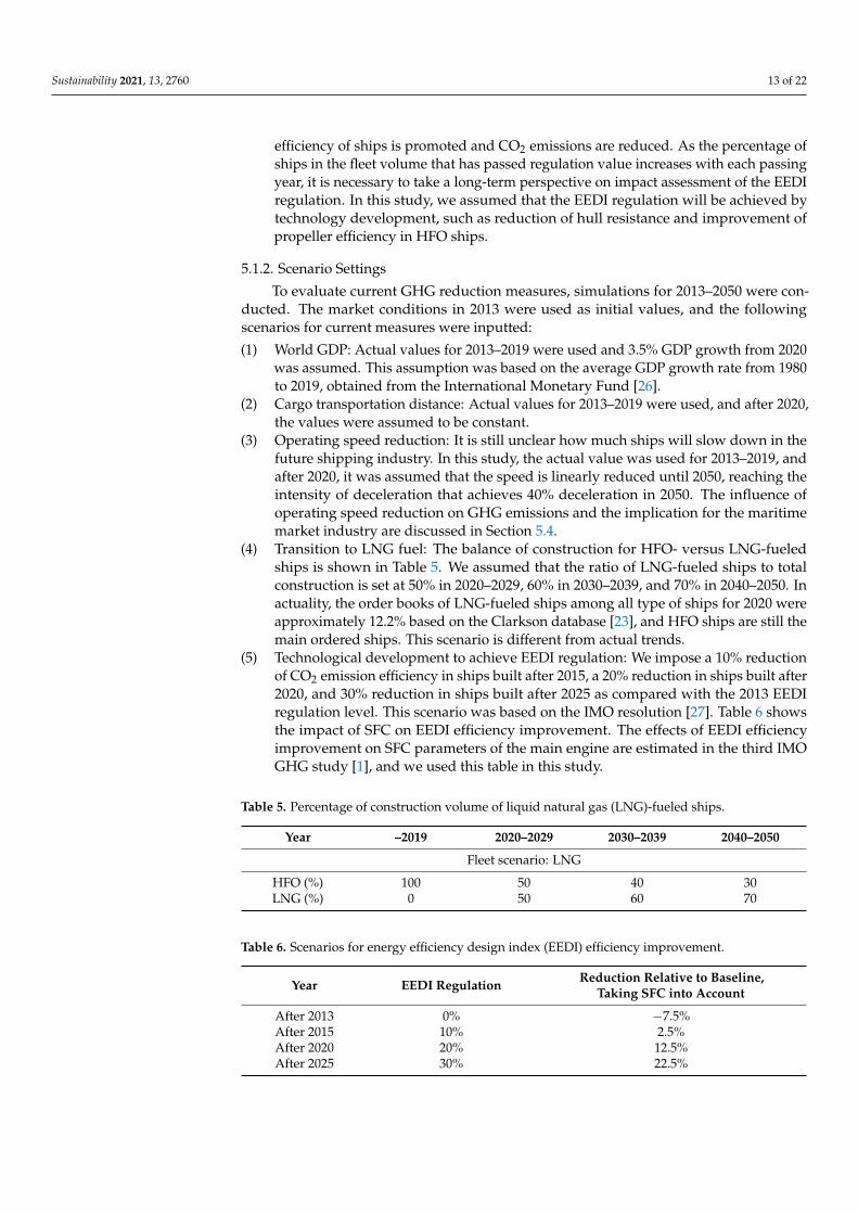
(4) Transition to LNG fuel: The balance of construction for HFO- versus LNG-fueledships is shown in Table 5. We assumed that the ratio of LNG-fueled ships to totalconstruction is set at 50% in 2020–2029, 60% in 2030–2039, and 70% in 2040–2050. Inactuality, the order books of LNG-fueled ships among all type of ships for 2020 wereapproximately 12.2% based on the Clarkson database [23], and HFO ships are still themain ordered ships. This scenario is different from actual trends.
(5) Technological development to achieve EEDI regulation: We impose a 10% reductionof CO2 emission efficiency in ships built after 2015, a 20% reduction in ships built after2020, and 30% reduction in ships built after 2025 as compared with the 2013 EEDIregulation level. This scenario was based on the IMO resolution [27]. Table 6 showsthe impact of SFC on EEDI efficiency improvement. The effects of EEDI efficiencyimprovement on SFC parameters of the main engine are estimated in the third IMOGHG study [1], and we used this table in this study.
Table 5. Percentage of construction volume of liquid natural gas (LNG)-fueled ships.
Year –2019 2020–2029 2030–2039 2040–2050
Fleet scenario: LNG
HFO (%) 100 50 40 30LNG (%) 0 50 60 70
Table 6. Scenarios for energy efficiency design index (EEDI) efficiency improvement.
Year EEDI Regulation Reduction Relative to Baseline,Taking SFC into Account
To evaluate these GHG reduction effects, the following evaluation criteria were established:
• Business as usual (BAU) lines: The base year for CO2 emissions is set as 2008 based onthe initial IMO strategy for reduction of GHG emissions from ships [22]. The BAUlines indicate that some GHG reduction measures have not been applied since 2008.The BAU lines are calculated using the model proposed in this study.
• Mid-term goal: In the initial strategy for reducing GHG emissions [22], the goal ofhalving GHG emissions by 2050 was decided based on 2008. Based on this strategy, amid-term goal of 50% reduction of CO2 emissions of bulk carriers by 2050 as comparedwith 2008 was set. CO2 emissions of bulk carriers in 2008 were 194.0 × 10⁶ tons basedon the third IMO GHG study [1]. Therefore, the mid-term goal is set at 97.0 × 10⁶ tonsin this study. It should be noted that CO2 emissions of bulk carriers were 193.4 × 10⁶
tons in 2018. Comparing the CO2 emissions in 2018 and 2008, no significant changewas found.
These evaluation criteria are original to this study and differ from the existing IMOcriteria. For example, the BAU lines of total CO2 emissions considering several types ofships (for example, bulk carriers, tankers, container ships, general cargo ships, and LNGships, among others) were shown in the fourth IMO GHG study [4]. However, the BAUlines in the IMO’s study were considered as the influence of GHG emission measures, andthe evaluation of the CO2 reduction effect of each measure is difficult using the IMO’s BAUlines. Therefore, the BAU lines in this study were simulated using the proposed model andutilized as a baseline to evaluate the reduction in CO2 emissions quantitatively by severalemission measures. The BAU lines simulated using the proposed model are different fromthose in the IMO’s study.
5.1.3. Simulation Results for Current Measures
In this simulation, we analyzed the CO2 emission reduction effect of the currentmeasures alone. The simulation results of CO2 emissions considering operating speedreduction, the transition to LNG fuel, and technological development to achieve EEDIregulation are shown in Figure 7. In the case of the BAU scenario, CO2 emissions willincrease approximately 3.3 times by 2050 with respect to 2008 CO2 emissions. This isbecause the influence of HFO ships increases with an increase in sea cargo movement. Inthe case of operating speed reduction, CO2 emissions decrease by 56.1% with respect toBAU lines by 2050. In the case of EEDI, CO2 emissions decrease by 24.3% with respect toBAU lines by 2050. In the case of transition to LNG fuel, CO2 emissions decrease by 14.6%with respect to BAU lines by 2050. As a result, operating speed reduction more effectivelyreduces emissions compared with EEDI efficiency improvement and the transition to LNGfuel. However, it is difficult to achieve the mid-term goals of 50% decrease with respectto 2008 CO2 emissions using a single measure alone; instead, it is necessary to combinemeasures. Based on these results, we considered deceleration of operating speed, transitionto LNG fuel, and technological development to achieve EEDI regulation.
5.2. Impact Assessment of Future Measures5.2.1. Scenario Settings
To examine measures to reduce GHG emissions that achieve the mid-term goal, onenew measure, the introduction of zero-emission ships, was introduced and evaluated forafter 2030. The initial values are the same as those in Section 5.1.2. The additional measuresincorporated are as follows:
• Introduction of zero-emission ships: Zero-emission ships use hydrogen (H2) fuel,ammonia (NH3) fuel, or other alternatives. By using these fuels, GHG emissionsfrom shipping become zero and significant reductions of GHG emissions are realizedcompared with current measures.
Two types of scenarios to introduce zero-emission ships (low case and high case) areconstructed and assumed to change the fleet composition if implemented. The scenarios are
Sustainability 2021, 13, 2760 15 of 22
listed in Table 7. We assume that only HFO fuel ships are constructed until 2019. After 2020,the construction of LNG-fueled ships begins. After 2030, the construction of zero-emissionships begins. Each number shows the ratio of fuel ship types to be built. This percentageapplies to the ships that are constructed, and the ships are added to the fleet composition.The scenarios of GDP and cargo transportation distance scenarios follow in Section 5.1.2.
Figure 7. Simulation results of CO2 emissions considering current measures. LNG, liquid naturalgas; EEDI, energy efficiency design index; BAU, business as usual.
Table 7. Percentage of construction volume of alternative fuels. HFO, heavy fuel oil; LNG, liquidnatural gas.
Year –2019 2020–2029 2030–2039 2040–2050
Fleet Scenario: Low
HFO (%) 100 20 10 0LNG (%) 0 80 60 30
Zero-Emission Fuel (%) 0 0 30 70
Fleet Scenario: High
HFO (%) 100 20 0 0LNG (%) 0 80 40 10
Zero-Emission Fuel (%) 0 0 60 90
5.2.2. Evaluation Results with Future Measures
In this simulation, we analyzed the CO2 emission reduction effect of the introduc-tion of zero-emission ships alone. The simulation results of CO2 emissions consideringintroduction of zero-emission ships are shown in Figure 8. The reduction effect of theintroduction of zero-emissions ships is considerably larger than that of other measures;CO2 emissions decrease by 57.9% in the low scenario with respect to BAU lines by 2050and by 75.4% in the high scenario with respect to BAU lines by 2050, because the ratio ofzero-emission ships to fleet volume directly contributes to the reduction of CO2 emissions.If all ships are replaced by zero-emission ships, CO2 emissions will be fully eliminated;however, replacing all ships would be difficult given the immature state of zero-emissiontechnology, and thus introduction of zero-emission ships fluctuates greatly depending onthe (projected) status of technology development.
Sustainability 2021, 13, 2760 16 of 22
Figure 8. Simulation results of CO2 emissions considering the introduction of zero-emission ships.
5.3. Impact Assessment of Combination of Current and Future Measures5.3.1. Scenario Settings
The simulation combines current measures (operating speed reduction, technologicaldevelopment to achieve EEDI regulation, and transition to LNG fuel) and future measures(introduction of zero-emission ships). The purpose of this simulation is to quantitativelygrasp the CO2 reduction effect when current and future measures are combined. In addition,we consider the scenarios to satisfy the mid-term goal for 2050. The following assumptionswere used in this simulation.
• Technological development to achieve EEDI regulation is applied to HFO and LNG-fueled ships.
• Reduction in operating speed applies to HFO and LNG-fueled ships; zero-emissionships are not the target of operating speed reduction, which thus does not occur forthem. This is because zero-emission ships are more efficient with regards to CO2emissions compared with HFO and LNG-fueled ships. Additionally, LNG-fueledships are more efficient in terms of CO2 emissions than HFO fuel ships. Therefore, thespeed of LNG-fueled ships is 10% faster than that of HFO ships. This assumption isbased on the concepts of energy efficiency existing ship index (EEXI) regulation [28].
In this simulation, we consider the four types of cases shown in Table 8. The scenarioof GDP and cargo transportation distance is the scenario in Section 5.1.2. The operatingspeed reduction was set to reach 40% deceleration in 2050 based on HFO fuel ships. In thelow and high scenarios, the deceleration rate is set to 17% and is constant after 2020.
Table 8. The scenario for simulation of combination of current and future measures. EEDI, energy efficiency design index.
Scenario Name Fleet Scenario Operating SpeedDeceleration Scenario
5.3.2. Evaluation Results for Combination of Current and Future Measures
The simulation results of CO2 emissions for the combination of current and futuremeasures are shown in Figure 9. In the current scenario, CO2 emissions in 2050 are207.3 × 106 tons. On the other hand, in the case where only the 40% operating speedreduction measure is applied, the CO2 emission amount becomes 277.6 × 10⁶ tons as of2050. Compared with these results, CO2 emissions are thus reduced by 70.3 × 10⁶ tonsby EEDI efficiency improvement and transition to LNG fuel. However, it is difficult toachieve mid-term goals by 2050. From these results, it is found that the introduction ofzero-emission ships is necessary to achieve mid-term goals.
Figure 9. Simulation results of CO2 emissions for the combination of current and future measures.
In the case of low scenarios, if zero-emission measures are promoted after 2030 inaddition to the current measures, it is difficult to achieve the mid-term goal by 2050;conversely, in high scenarios, the 2050 goal can be achieved. Similarly, in the low + slowscenarios, it is possible to achieve mid-term goals. Therefore, it is necessary to consider thetransition to LNG fuel, introduction of zero emissions ships, deceleration operation, andtechnological development to achieve EEDI regulation from a long-term perspective.
The simulation scenario is set such that LNG fuel will be introduced from 2020, and azero-emission ship is introduced from 2030. This scenario is extremely difficult to realizein relation to reality. Based on the above, to promote GHG reduction, it is necessary notonly to promote the development of zero-emission ships, but also to implement additionalGHG emission schemes such as market-based measures.
From the results, it can be seen that the influence of the combination of all measureson CO2 emissions was considered.
5.4. Limitation of Operating Speed Reduction
It is clear that the ship operating speed reduction is effective in CO2 emissions re-duction from the results in Section 5.1.3. However, if excessive deceleration operationis performed, the required fleet quantity will increase sharply. In this simulation, thelimit of deceleration is considered using the proposed model. The scenario of GDP andcargo transportation distance is the scenario of Section 5.1.2, and the cases of decelerationoperation are four cases of 20%, 40%, 50%, and 70%.
The simulation results of CO2 emissions considering deceleration operation are shownin Figure 10. In the case of 20%, 40%, and 50% deceleration, CO2 emissions decrease
Sustainability 2021, 13, 2760 18 of 22
as the ship speed decreases. In the case of a 70% deceleration, CO2 emissions decreaseprogress until 2038. However, CO2 emissions increased from 2039 because of an increase inshipbuilding orders.
Figure 10. Simulation results of CO2 emissions considering deceleration operation.
The results under the impact of increases in fleet volume and shipbuilding orders areshown in Figure 11. Both fleet volume and orders increase as the deceleration strengthincreases. This is the influence of the correction of the order prediction model (Section 3.4).By increasing the operating speed decelerations, it is expected that ship orders will alsoincrease, and the shipbuilding industry can benefit. Especially in the case of a 70% decel-eration, orders increase rapidly and fluctuate from 2033, and the fleet volume increasesrapidly after 2039. This rapid increase in ship orders is caused by a significant shortageof ship capacity due to rapid deceleration. Although 70% had excessive deceleration,CO2 emissions increased gradually as the fleet increased. The engine load factor is verysmall (less than 5%); therefore, CO2 emissions increase gradually compared with the fleetincrease. The fleet volume becomes insufficient, and marine transportation has failed tomeet demand because of a significant shortage of fleet volume in 70% deceleration, and70% deceleration is difficult from a maritime transportation perspective. From these results,it was found that the limitation of deceleration in ship operations was approximately 50%.
Figure 11. Simulation results for fleet volume and shipbuilding orders.
Sustainability 2021, 13, 2760 19 of 22
We also showed that, by combining such a model of GHG emissions with a modelof the shipping and shipbuilding market, the effect of reducing GHG emissions can beanalyzed based on dynamic changes in the market.
5.5. Discussion
In Section 5.1, we conducted a quantitative evaluation of the current measures forCO2 emission reduction, especially deceleration operation, transition to LNG fuel, andtechnological development, to achieve EEDI regulation. The result suggests that thedeceleration operation had the highest CO2 reduction effect, followed by technologicaldevelopment to achieve EEDI regulation and transition to LNG fuel. In particular, theCO2 emission reduction effect by the deceleration operation considers change in ordersand scrap due to the operating speed reduction; few or no evaluations that considerthe maritime market aspect have been conducted in previous studies. By modeling therelationship between operation speed and number of orders and between operation speedand amount of scrap, our model enables this consideration.
In Section 5.2, we evaluated the introduction of zero-emission ships for CO2 emissionreduction. The result demonstrates that our model can forecast the impact of the futureintroduction of zero-emission ships, considering the transition from current ships. In thesimulation, we assumed two scenarios of the introduction of zero-emission ships andevaluated the amount of CO2 emission reduction by the introduction. However, AmericanBureau of Shipping [29] has reported that zero-emission ships are still at the researchstage, and the scenario for their introduction has not become clear yet. The introduction ofzero-emission ships greatly depends on the projected status of technology development,thus it is necessary to carefully consider what scenarios should be evaluated.
In Section 5.3, we evaluated the combination of current and future measures for CO2emission reduction. In the simulation, EEXI measures for existing ships are also taken intoconsideration. The result shows that it is difficult to achieve the IMO goals for 2050 bycombining only current measures. Additionally, the result shows that the target for 2050can be achieved in the “high“ scenario, which introduces many zero-emission ships, or the“low + slow” scenario, which introduces zero-emission ships and deceleration operation.In the “high” scenario, zero-emission ships account for 60% of ships constructed from 2030;achieving this is considered difficult at the present stage of development of zero-emissionships. The “low + slow“ scenario is considered to be more realistic from the perspective ofachieving IMO goals for 2050; however, the amount of LNG-fueled ships on order booksfor all ship types is only approximately 12.2% as of 2020 [23], which is still lower than theassumption of the “low + slow” scenario. Based on these considerations, it is necessary notonly to promote the development of zero-emission ships, but also to implement additionalGHG emission schemes such as market-based measures.
In the fourth IMO GHG study [4], future CO2 emissions are predicted. It is reportedthat CO2 emissions in 2050 will be approximately 90–130% compared with 2008 owing todeceleration operation, EEDI efficiency improvement, improvement of operation efficiency,and so on. This result can be interpreted to show that additional measures, such as theintroduction of zero-emission ships and market-based measures, are required to achievethe 2050 GHG emission target. The “current” scenario in Figure 9 confirms the effectivenessof the current measures and shows that the case where only current measures are combinedmakes it difficult to achieve the 2050 GHG emission target. The results of the forth IMOstudy and the simulation results in this study are qualitatively consistent. This paperis novel in that we considered multiple scenarios—“high” and “low + slow”—and thesimulation results suggest some example roadmaps for the implementation of the IMO’sGHG reduction strategy. Those examples can serve as reference data to discuss the futuredevelopment of decarbonized shipping, and this is one of the important contributions ofthis paper.
In Section 5.4, we considered the limitation of deceleration operation and the ef-fectiveness of combining shipping and shipbuilding market models and GHG emission
Sustainability 2021, 13, 2760 20 of 22
prediction models. In this simulation, we analyzed the limit of deceleration operation fromthe maritime market perspective and showed that the limit of deceleration operation isapproximately 50%. Previous studies cannot consider this limitation because their modelsdo not combine GHG emission prediction and maritime market models. This case sug-gests the importance of considering the maritime market when evaluating the effect ofdeceleration, and this consideration is also part of the novelty of our model.
The simulations in Sections 5.1–5.4 demonstrate that our model can analyze dynamicsin the maritime market when GHG emission measures are implemented. The resultscan be used for the establishment of international rules such as IMO rules and for policymaking in maritime governance. Specifically, it will be possible to study a scenario with theintroduction of zero-emission ships and to analyze market fluctuations due to regulationson existing ships such as EEXI regulation [28].
6. Conclusions
In this study, a model to consider GHG emission scenarios for the maritime trans-portation sector was developed using SD. Using this model, the influence of several GHGemissions reduction scenarios was examined. Additionally, several simulations were exe-cuted using the proposed model, and we evaluated the impacts of several measures onGHG emissions. Then, we built a theoretical framework to develop a model that compre-hensively evaluates the impact of GHG reduction measures in the maritime market. Theconclusions can be summarized as follows:
• To estimate GHG emissions, a GHG emissions prediction model was developed andthe scrap model was improved. Additionally, the GHG emissions prediction modelwas integrated into shipping and shipbuilding market models, and a model to considerGHG reduction measures was developed.
• To confirm the validity of the evaluation model for GHG reduction measures, simulationsfrom 2013 to 2018 were conducted. The model validity was confirmed quantitatively.
• The GHG emission reduction effect by current measures and future measures alonewas evaluated. Additionally, the impact and effectiveness of combining currentmeasures and future measures were evaluated.
• The comprehensive scenarios to achieve IMO GHG emission goals were discussedconsidering current and future GHG reduction measures. From this simulation result,it was found that, in order to achieve the target of 2050, it is necessary to develop azero-emission ship in addition to the current measures.
• We focused on the deceleration of operating speed, the influence of which on shippingand shipbuilding markets was evaluated. Concretely, the limitation of decelerationwas considered from the maritime market perspective. This simulation result suggeststhat the limitation of ship operating speed reduction is approximately 50% from themaritime market perspective.
However, on the other hand, the developed model is still insufficient for cost calcu-lation. Concretely, measures to reduce GHG emissions affect ship operating costs andship prices. However, the influences of ship operating costs and ship prices have not beenconsidered in this study. In future work, we will expand the model to simulate theseitems, and develop a model to consider optimal scenarios in terms of the balance betweenmaritime market and GHG emissions. Additionally, the proposed model predicts theamount of sea cargo movement using GDP and cargo transportation distance. However, itis difficult to accurately predict these values because of the uncertainties involved. In futurework, we are considering how to handle these uncertainties. The sophistication of theshipping and shipbuilding market model is also an issue for future work. In recent years,it has become possible to grasp the ship movement in real time by development of AISand to obtain detailed cargo flow volume of dry bulk cargo based on ship movement [30].By using such ship movement data, it is expected that sophisticated cargo transportationvolume data will be achievable and the shipping and shipbuilding market model in thisstudy will improve as a predictive tool.
Sustainability 2021, 13, 2760 21 of 22
Author Contributions: Conceptualization, Y.W.; methodology, Y.W. and T.Y.; software, Y.W. and T.Y.;validation, Y.W., T.Y., K.H., and S.W.; formal analysis, Y.W. and T.Y.; investigation, Y.W., T.Y., andS.W.; writing—original draft preparation, Y.W. and T.Y.; writing—review and editing, Y.W., T.Y., K.H.,and S.W.; visualization, Y.W. and T.Y.; funding acquisition, Y.W., K.H., and S.W. All authors have readand agreed to the published version of the manuscript.
Funding: This work was supported by JSPS KAKENHI Grant Numbers JP19K15233, JP20H02371,JP20K14967, and JP20H00286.
Data Availability Statement: Some of the data presented in this study are openly available inreference number [1,4,23–27].
Conflicts of Interest: The authors declare no conflict of interest in this paper.
L.; et al. Third IMO Greenhouse Gas Study 2014; International Maritime Organization: London, UK, 2015.2. Komiyama, R.; Suzuki, K.; Nagatomi, Y.; Matsuo, Y.; Suehiro, S. Analysis of Japan’s energy demand and supply to 2050 through
integrated energy-economic model. J. Jpn. Soc. Energy Resour. 2012, 33, 34–43. (In Japanese)3. Holz, C.; Siegel, L.; Johnston, E.; Jones, A.; Sterman, J. Ratcheting ambition to limit warming to 1.5 ◦C: Trade-offs between
emission reductions and carbon dioxide removal. Environ. Res. Lett. 2018, 13, 064028. [CrossRef]4. IMO: Fourth IMO GHG Study 2020, IMO MEPC 75/7/15. 2020. Available online: https://docs.imo.org/ (accessed on 6
August 2020).5. Faber, J.; Markowska, A.; Eyring, V.; Cionni, I.; Selstad, E. A Global Maritime Emissions Trading System—Design and Impacts on the
Shipping Sector, Countries and Regions; CE Delft: Delft, The Netherlands, 2010.6. Lindstad, E.; Rialland, A. LNG and cruise ships, an easy way to fulfil regulations—versus the need for reducing GHG emissions.
Sustainability 2020, 12, 2080. [CrossRef]7. Rehmatulla, N.; Calleya, J.; Smith, T. The implementation of technical energy efficiency and CO2 emission reduction measures in
shipping. Ocean Eng. 2017, 139, 184–197. [CrossRef]8. Kobayashi, M.; Hashiguchi, Y.; Sawada, N. Actual status of slow-down operation: Challenges, countermeasures, and results of
slow-down operation. J. Jpn. Inst. Mar. Eng. 2014, 49, 74–80. (In Japanese) [CrossRef]9. Smith, T.W.P. Technical energy efficiency, its interaction with optimal operating speeds and the implications for the management
of shipping’s carbon emissions. Carbon Manag. 2012, 3, 589–600. [CrossRef]10. Nielsen, K.S.; Kristensen, N.E.; Bastiansen, E.; Skytte, P. Forecasting the market for ships. Long Range Plan. 1982, 15, 70–75.
[CrossRef]11. Sakalayen, Q.M.H.; Duru, O.; Hirata, E. An econophysics approach to forecast bulk shipbuilding orderbook: an application of
Newton’s law of gravitation. Marit. Bus. Rev. 2020. [CrossRef]12. Gourdon, K. An Analysis of Market-Distorting Factors in Shipbuilding: The Role of Government interventions, OECD Science, Technology
and Industry Policy Papers; OECD Publishing: Paris, France, 2019; Volume 67.13. Shin, J.; Lim, Y.-M. An empirical model of changing global competition in the shipbuilding industry. Marit. Policy Manag. 2014,
41, 515–527. [CrossRef]14. Taylor, A.J. The dynamics of supply and demand in shipping. Dynamica 1975, 2, 62–71.15. Japan Maritime Research Institute SD Study Group. SD model of maritime transportation and shipbuilding. Jpn. Marit. Res. Inst.
Bull. 1978, 142. (In Japanese)16. Engelen, S.; Meersman, H.; Eddy, V.D.V. Using system dynamics in maritime economics: An endogenous decision model for ship
owners in the dry bulk sector. Marit. Policy Manag. 2006, 33, 141–158. [CrossRef]17. Wada, Y.; Hamada, K.; Hirata, N.; Seki, K.; Yamada, S. A system dynamics model for shipbuilding demand forecasting. J. Mar.
Sci. Technol. 2018, 23, 236–252. [CrossRef]18. Forrester, J.W. Industrial Dynamics; MIT Press: Cambridge, MA, USA, 1961.19. Sterman, J. Business Dynamics: Systems Thinking and Modeling for a Complex World; Irwin Professional Publishing: Burr Ridge, IL,
USA, 2000.20. Sterman, J.; Fiddaman, T.; Franck, T.R.; Jones, A.; McCauley, S.; Rice, P.; Sawin, E.; Siegel, L. Climate interactive: The C-ROADS
climate policy model. Syst. Dyn. Rev. 2012, 28, 295–305. [CrossRef]21. Wada, Y.; Hamada, K.; Hirata, N. A Study on the Improvement and Application of System Dynamics Model for Demand
Forecasting of Ships. In Proceedings of the International Conference on Computer Applications in Shipbuilding, 1, Singapore,26–28 September 2017; pp. 51–60.
22. IMO MEPC72. Resolution MEPC.304(72). Initial IMO Strategy on Reduction of GHG Emissions from Ships. 2018. Availableonline: https://wwwcdn.imo.org/localresources/en/KnowledgeCentre/IndexofIMOResolutions/MEPCDocuments/MEPC.304(72).pdf (accessed on 21 January 2021).
23. Clarksons Shipping Intelligence Network. Available online: http://www.clarksons.net (accessed on 6 February 2021).
24. Sea-Web Ships. Available online: https://maritime.ihs.com/Account2/Index (accessed on 8 December 2019).25. Buhaug, Ø.; Corbett, J.J.; Endresen, Ø.; Eyring, V.; Faber, J.; Hanayama, S.; Lee, D.S.; Lee, D.; Lindstad, H.; Markowska, A.Z.; et al.
Second IMO GHG Study 2009; International Maritime Organization (IMO): London, UK, 2009.26. International Monetary Fund. Available online: https://www.imf.org/external/datamapper/NGDP_RPCH@WEO/
WEOWORLD (accessed on 17 January 2021).27. IMO MEPC 62/24/Add.1, ANNEX 19 RESOLUTION MEPC.203(62), 2011. Available online: https://wwwcdn.imo.org/
localresources/en/OurWork/Environment/Documents/Technical%20and%20Operational%20Measures/Resolution%20MEPC.203(62).pdf (accessed on 7 December 2020).
28. Japan Ship Technology Research Association; Ministry of Land, Infrastructure, Transport and Tourism. Roadmap to Zero Emissionfrom International Shipping; Ministry of Land, Infrastructure, Transport and Tourism: Tokyo, Japan, 2020.
29. American Bureau of Shipping (ABS). Ammonia as Marine Fuel; ABS Sustainability Whitepaper; 2020. Available online: https://absinfo.eagle.org/acton/fs/blocks/showLandingPage/a/16130/p/p-0227/t/page/fm/0 (accessed on 7 December 2020).
30. Kanamoto, K.; Murong, L.; Nakashima, M.; Shibasaki, R. Can maritime big data be applied to shipping industry analysis?Focussing on commodities and vessel sizes of dry bulk carriers. Marit. Econ. Logist. 2020. [CrossRef]