Evaluation of Textural Features for Multispectral Images Ulya Bayrama, Gulcan Canb, Sebnem Duzgunc, Nese Yalabikd
aC3S Ltd. Command Control & Cybernetic Systems, ODTU Teknokent, Ankara, Turkey; bDept. of Computer Engineering, Middle East Technical Univ./Ankara, Turkey;
cDept. of Mining Engineering and Geodetic & Geographic Inf. Tech., Middle East Technical Univ./Ankara, Turkey;
dYalabik Engineering Company ODTU Teknokent, Ankara, Turkey
ABSTRACT
Remote sensing is a field that has wide use, leading to the fact that it has a great importance. Therefore performance of selected features plays a great role. In order to gain some perspective on useful textural features, we have brought together state-of-art textural features in recent literature, yet to be applied in remote sensing field, as well as presenting a comparison with traditional ones. Therefore we selected most commonly used textural features in remote sensing that are grey-level co-occurrence matrix (GLCM) and Gabor features. Other selected features are local binary patterns (LBP), edge orientation features extracted after applying steerable filter, and histogram of oriented gradients (HOG) features. Color histogram feature is also used and compared. Since most of these features are histogram-based, we have compared performance of bin-by-bin comparison with a histogram comparison method named as diffusion distance method. During obtaining performance of each feature, k-nearest neighbor classification method (k-NN) is applied.
Keywords: Gray level co-occurrence matrix, histogram of oriented gradients, Gabor feature, linear binary pattern, color histogram, diffusion distance, textural features, remote sensing
1. INTRODUCTION There is extensive work on texture analysis in the literature. Although texture analysis has study areas in corporation with segmentation, image synthesizing, and shape cue extraction, it has been applied to classification problems more commonly15. This is due to varying application areas such as medical image analysis and remotely-sensed data analysis15.
In texture classification, representativeness of features is crucial. Textural features have a common property to reflect the spatial configuration of a pattern beyond color-related features. Thus, they can capture class-specific patterns and have the ability to discriminate similar or close-colored patterns. From this perspective, they can be used to represent objects as well.
In remote sensing area, textural features are used most widely for land use/land cover classification as well as object detection. With availability of high resolution satellite data, characteristics of remote sensing objects or fields can be analyzed further. Differences between two forest types would be realistically tractable for instance. Thus, representation capability of textural features gains importance in that sense.
Formerly, textural features were examined in a statistical manner. Features adopted from those times can be counted as gray-level co-occurrence matrix method1,7 and filtering based approaches like Gabor filters7,8,9,10 and wavelet transform21, 22. Although these approaches can give really good results with similar training and test data, they seem to suffer as within-class variance gets high or rotation problem gets involved15. Since remote sensing data is highly-variant, can contain complex structures and patterns learned can be in any directions, more representative features are desired.
Recent approaches emerged from the need of rotation, scale and affine invariance, better demonstration and discrimination of similar classes etc. These approaches include local binary pattern (LBP)2, local edge pattern (LEP)2, histogram of oriented gradients5 (HOG) and edge orientation extraction2. Ojala et al. states that LBP feature can capture spatial configuration of pattern very well, yet it would be best to combine it with variance
difference (VAR) feature for a full representation16. Guo et al. asserts that LBP/VAR feature consider variance difference in a global sense, yet it should be local as well. Thus they propose LBPV for local representation of spatial arrangement as well as contrast difference15. HOG feature is proposed by Dalal and Triggs for human detection task5, and recently used for car detection in remote sensing as well12, 13. It captures texture by filtering the image and features are obtained by combining histograms of gradient directions taken from image tiles. Edge orientation is favorable since it is used in similar land use land cover classification tasks and seems to be able to differentiate man-made and natural structures2, 3. Edge responses are obtained by applying steerable filter beforehand4. In order to make extracted edge orientation features rotation invariant fast Fourier transform is used afterwards2, 3.
Most of these features are histogram-based and should be treated accordingly during classification. There are approaches which treat histograms as a whole instead of just comparing each feature (each histogram bin) independently. Most popular approach for histogram comparison is Kullback-Leibler divergence which measures how dissimilar two probability density functions14. For this purpose, we have chosen a fairly new and robust dissimilarity measure called diffusion distance6. It is proposed by Ling and Okada for histogram-based local descriptors. Diffusion distance is asserted to be robust to deformation, lighting change and noise, since it is a cross-bin histogram distance6.
In this study, we have analyzed how successfully land use/land cover classification can be carried out with varying textural features. Primarily, we have analyzed selected textural features for their representativeness on remote sensed images. Secondly, we have compared feature by feature classification and histogram-based classification. Dataset used for experiments in this study is explained in Section 2 with demonstrations of example train and test images. Implementation or usage details of features are explained further in Section 3. Details of classification methods and analysis of results can be found in the ongoing corresponding parts of the paper. In the end, we draw conclusions and mention future work in this area.
2. DATASET
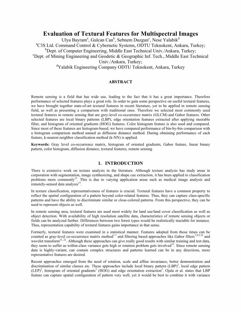
Figure 1. Training and test images of classes; water, urban, forest and cropland
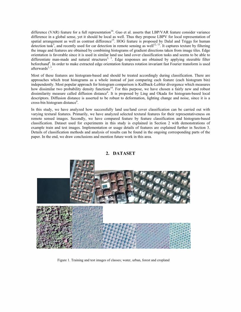
Figure 2. PCA plot of GLCM features for four classes
Train and test data are extracted from high-resolution (0.6 m) images of Quickbird satellite from Fethiye in Turkey. These multispectral images contain four bands that are red, green, blue and near-infrared. Anderson et. al. categorized areas in remote sensed images for land use/land cover (LULC) classification24, and in the proposed work, some of the main classes (from Level 1) are studied according to their availabilities in the dataset. Selected classes are water, urban, forest and cropland in this study. During first tests, bare land class was selected instead of cropland, however owing to the lack of available bare land areas in satellite images of Fethiye and these bare areas not having a specific texture, this class is replaced with cropland. Some of the selected field patches can be seen from Figure 1. In order to obtain many test and train images, these large patches are divided into smaller patches. Among these small patches, only the ones that represents the class are selected, which means that for example from an image patch of urban class, small patch that contains a swimming pool is not selected. 200 training images are collected that has 50 images for each class. Test images are collected from the rest that are 50 for water, 32 for urban, 77 for forest and 46 for cropland classes. The number of test images varies for each class depending on the availability of them in satellite images of Fethiye.
3. TEXTURAL FEATURES 3.1 Gray Level Co-Occurrence Matrix (GLCM)
GLCM is one of the traditional textural features as this is the most popularly selected feature for classification of remotely sensed images that is also known as spatial dependency matrix. This method is proposed by Haralick in 1973 as a distribution of co-occurring pixel values at a given offset over the image1, 7. More specifically, GLCM is a matrix that shows how often a pixel with gray-level value i occurs adjacent to a pixel with value j. Selection of offset defines the neighboring pixel location; so use of many offsets give the feature rotation invariance. However GLCM is only a representation of the texture, therefore in order to extract a feature from this representation; additional calculations are necessary. There are a number of features available for GLCM such as; contrast (variance), correlation, energy (uniformity, angular second moment) and homogeneity1, 7.
In the proposed work, we selected GLCM as it is commonly used in remote sensed data classification depending on its high performance. In the calculation of GLCM, we selected 8-neighborhood as offset in order to obtain rotation invariance; therefore GLCM is calculated in four directions (00, 450, 900, 1350) separately. After GLCM’s are calculated in four directions, contrast, energy and homogeneity features are extracted. During this process, we preferred not to select correlation feature since it gives not-a-number (NaN) values for constant images, therefore it would not be representative for constant classes such as water class in our case. Concatenation of three features calculated for four directions gives a feature vector with 12 elements for each band of the image. Therefore for four band images that we selected, final length of the feature vector is 48.
In order to see the visual separability, Principal Component Analysis (PCA) is operated on training dataset as can be seen from Figure 2. PCA shows that water class is easily separated from the rest; urban class is rather separable as well. However forest and crop classes don’t seem to be separated from each other with GLCM features as much. Further analysis can be observed from results section.
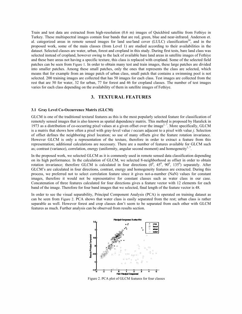
Figure 3. PCA plot of Gabor feature
3.2 Gabor Textural Feature
As mentioned previously for GLCM, Gabor feature is not a textural feature as well; rather it is a representation of the image texture. Gabor is a linear filter that is practical to represent edges therefore resulting filtered image embodies texture information. Filtering operation is directional, therefore in order to obtain rotation invariance, it is important to filter in multiple directions. After images are filtered by Gabor, resulting texture representation are used to obtain a feature vector. After images are filtered with various directions, features such as mean, energy, entropy, standard deviation can be extracted8, 9.
This feature is also one of the most popular textural features used for remote sensing8, 9; therefore we selected this feature as well. In the selected algorithm9, Gabor wavelets are generated primarily. As proposed in9, 4 scales and 6 directions are selected. Secondarily, images are filtered with wavelets resulting with a texture representation of the image. After the filtering process, we selected mean and standard deviation features as in9 since other features are already used for extraction of GLCM features. After mean and standard deviation of the texture representation is calculated for each band and results are concatenated, feature vector with length 192 is obtained. As can be seem from Figure 3, PCA of Gabor feature is more separable than GLCM feature.
3.3 Histogram of Oriented Gradients (HOG)
HOG feature is constructed for human detection by Dalal and Triggs5 that puts a grid on the image, evaluates normalized local histograms of image gradient directions. According to Dalal, best performance is taken by filtering the image with [-1 0 1] gradient filter with no smoothing. After filtering operation, 1D histogram of gradient directions of each grid cell is calculated and for the final representation, these histogram entries are combined as feature vector. In order to improve the performance, contrast normalization is applied to image beforehand. The advantage of this textural feature is that it captures general structure of the object. According to Dalal, HOG method is kind of a combination of edge orientation, SIFT and shape context, therefore it is told to be affective.
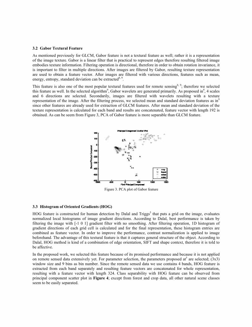
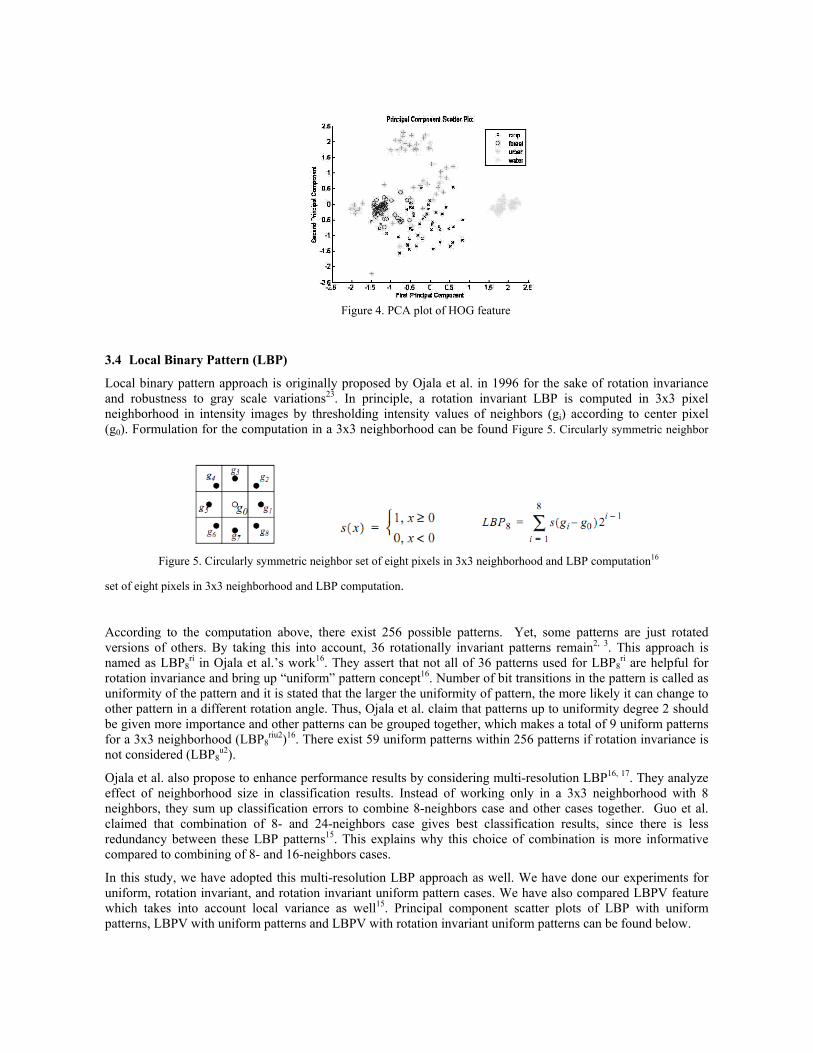
In the proposed work, we selected this feature because of its promised performance and because it is not applied on remote sensed data extensively yet. For parameter selection, the parameters proposed at5 are selected; (3x3) window size and 9 bins as bin number. Since the remote sensed data we use contains 4 bands, HOG feature is extracted from each band separately and resulting feature vectors are concatenated for whole representation, resulting with a feature vector with length 324. Class separability with HOG feature can be observed from principal component scatter plot in Figure 4; except from forest and crop data, all other natural scene classes seem to be easily separated.
Figure 4. PCA plot of HOG feature
3.4 Local Binary Pattern (LBP)
Local binary pattern approach is originally proposed by Ojala et al. in 1996 for the sake of rotation invariance and robustness to gray scale variations23. In principle, a rotation invariant LBP is computed in 3x3 pixel neighborhood in intensity images by thresholding intensity values of neighbors (gi) according to center pixel (g0). Formulation for the computation in a 3x3 neighborhood can be found Figure 5. Circularly symmetric neighbor
set of eight pixels in 3x3 neighborhood and LBP computation.
According to the computation above, there exist 256 possible patterns. Yet, some patterns are just rotated versions of others. By taking this into account, 36 rotationally invariant patterns remain2, 3. This approach is named as LBP8
ri in Ojala et al.’s work16. They assert that not all of 36 patterns used for LBP8 ri are helpful for
rotation invariance and bring up “uniform” pattern concept16. Number of bit transitions in the pattern is called as uniformity of the pattern and it is stated that the larger the uniformity of pattern, the more likely it can change to other pattern in a different rotation angle. Thus, Ojala et al. claim that patterns up to uniformity degree 2 should be given more importance and other patterns can be grouped together, which makes a total of 9 uniform patterns for a 3x3 neighborhood (LBP8
riu2)16. There exist 59 uniform patterns within 256 patterns if rotation invariance is not considered (LBP8
u2).
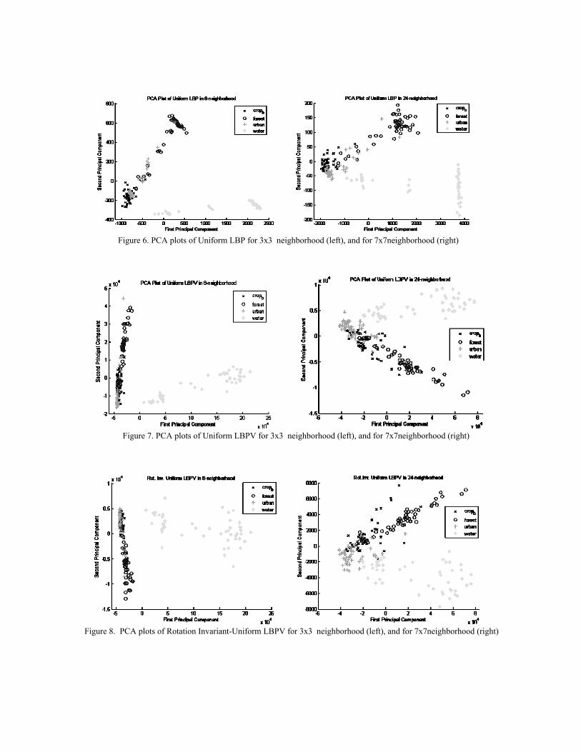
Ojala et al. also propose to enhance performance results by considering multi-resolution LBP16, 17. They analyze effect of neighborhood size in classification results. Instead of working only in a 3x3 neighborhood with 8 neighbors, they sum up classification errors to combine 8-neighbors case and other cases together. Guo et al. claimed that combination of 8- and 24-neighbors case gives best classification results, since there is less redundancy between these LBP patterns15. This explains why this choice of combination is more informative compared to combining of 8- and 16-neighbors cases.
In this study, we have adopted this multi-resolution LBP approach as well. We have done our experiments for uniform, rotation invariant, and rotation invariant uniform pattern cases. We have also compared LBPV feature which takes into account local variance as well15. Principal component scatter plots of LBP with uniform patterns, LBPV with uniform patterns and LBPV with rotation invariant uniform patterns can be found below.
Figure 5. Circularly symmetric neighbor set of eight pixels in 3x3 neighborhood and LBP computation16
Figure 6. PCA plots of Uniform LBP for 3x3 neighborhood (left), and for 7x7neighborhood (right)
Figure 8. PCA plots of Rotation Invariant-Uniform LBPV for 3x3 neighborhood (left), and for 7x7neighborhood (right)
Figure 7. PCA plots of Uniform LBPV for 3x3 neighborhood (left), and for 7x7neighborhood (right)
During our experiments, we have reduced four band of each image to single band by averaging and then applied normalization as recommended in Ojala’s study15. We have obtained histograms with different sizes for each case (uniform, rotation invariant and rotation invariant-uniform) due to varying number of possible patterns.
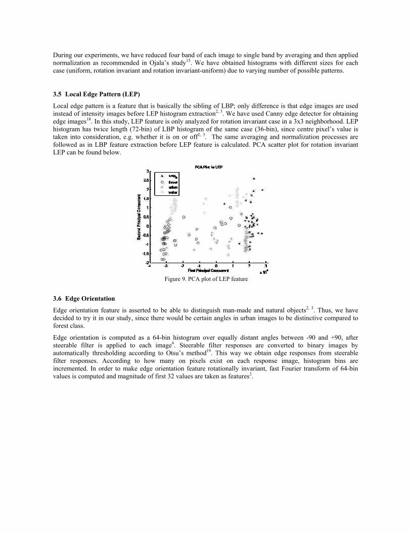
3.5 Local Edge Pattern (LEP)
Local edge pattern is a feature that is basically the sibling of LBP; only difference is that edge images are used instead of intensity images before LEP histogram extraction2, 3. We have used Canny edge detector for obtaining edge images18. In this study, LEP feature is only analyzed for rotation invariant case in a 3x3 neighborhood. LEP histogram has twice length (72-bin) of LBP histogram of the same case (36-bin), since centre pixel’s value is taken into consideration, e.g. whether it is on or off2, 3. The same averaging and normalization processes are followed as in LBP feature extraction before LEP feature is calculated. PCA scatter plot for rotation invariant LEP can be found below.
3.6 Edge Orientation
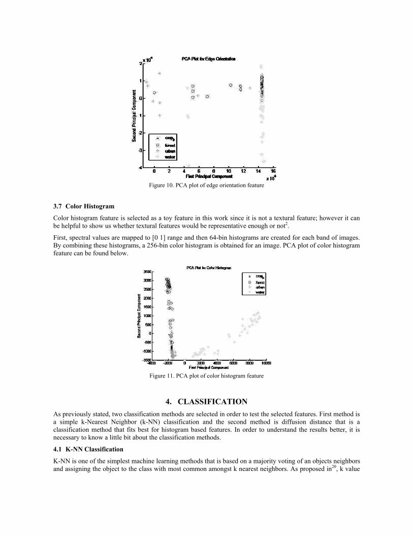
Edge orientation feature is asserted to be able to distinguish man-made and natural objects2, 3. Thus, we have decided to try it in our study, since there would be certain angles in urban images to be distinctive compared to forest class.
Edge orientation is computed as a 64-bin histogram over equally distant angles between -90 and +90, after steerable filter is applied to each image4. Steerable filter responses are converted to binary images by automatically thresholding according to Otsu’s method19. This way we obtain edge responses from steerable filter responses. According to how many on pixels exist on each response image, histogram bins are incremented. In order to make edge orientation feature rotationally invariant, fast Fourier transform of 64-bin values is computed and magnitude of first 32 values are taken as features2.
Figure 9. PCA plot of LEP feature
3.7 Color Histogram
Color histogram feature is selected as a toy feature in this work since it is not a textural feature; however it can be helpful to show us whether textural features would be representative enough or not2.
First, spectral values are mapped to [0 1] range and then 64-bin histograms are created for each band of images. By combining these histograms, a 256-bin color histogram is obtained for an image. PCA plot of color histogram feature can be found below.
4. CLASSIFICATION As previously stated, two classification methods are selected in order to test the selected features. First method is a simple k-Nearest Neighbor (k-NN) classification and the second method is diffusion distance that is a classification method that fits best for histogram based features. In order to understand the results better, it is necessary to know a little bit about the classification methods.
4.1 K-NN Classification
K-NN is one of the simplest machine learning methods that is based on a majority voting of an objects neighbors and assigning the object to the class with most common amongst k nearest neighbors. As proposed in20, k value
Figure 11. PCA plot of color histogram feature
Figure 10. PCA plot of edge orientation feature
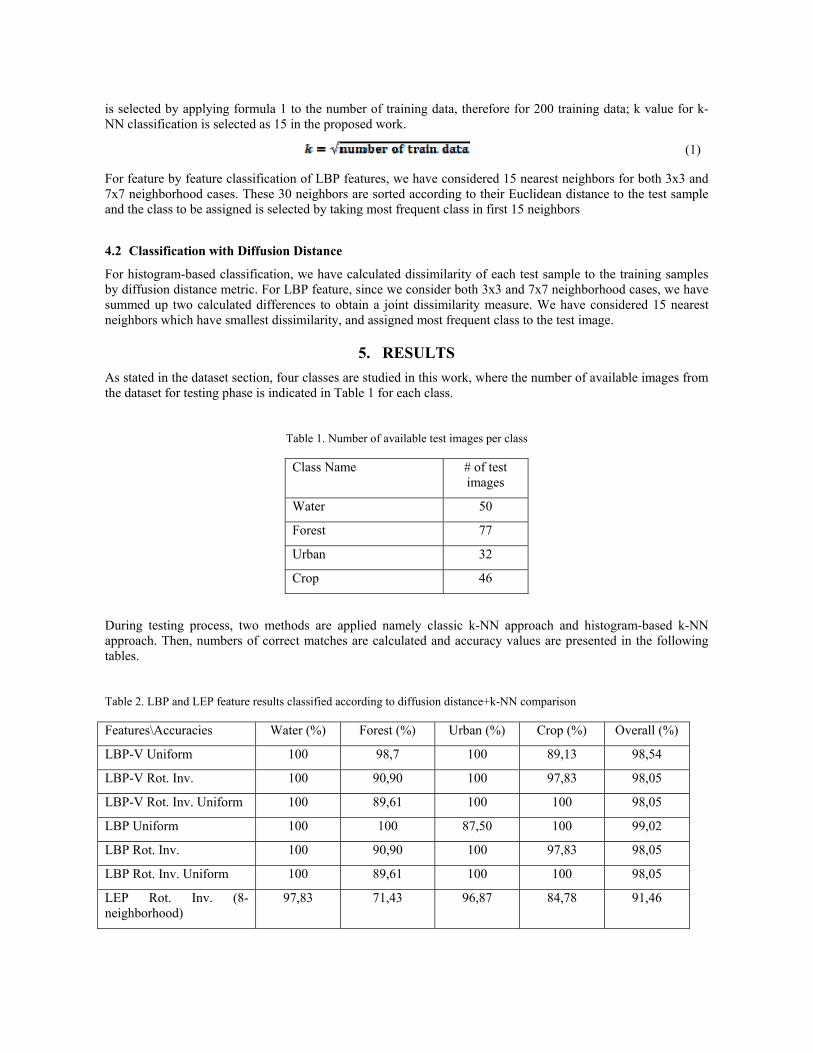
is selected by applying formula 1 to the number of training data, therefore for 200 training data; k value for k- NN classification is selected as 15 in the proposed work.
(1)
For feature by feature classification of LBP features, we have considered 15 nearest neighbors for both 3x3 and 7x7 neighborhood cases. These 30 neighbors are sorted according to their Euclidean distance to the test sample and the class to be assigned is selected by taking most frequent class in first 15 neighbors
4.2 Classification with Diffusion Distance
For histogram-based classification, we have calculated dissimilarity of each test sample to the training samples by diffusion distance metric. For LBP feature, since we consider both 3x3 and 7x7 neighborhood cases, we have summed up two calculated differences to obtain a joint dissimilarity measure. We have considered 15 nearest neighbors which have smallest dissimilarity, and assigned most frequent class to the test image.
5. RESULTS As stated in the dataset section, four classes are studied in this work, where the number of available images from the dataset for testing phase is indicated in Table 1 for each class.
Table 1. Number of available test images per class
Class Name # of test images
Water 50
Forest 77
Urban 32
Crop 46
During testing process, two methods are applied namely classic k-NN approach and histogram-based k-NN approach. Then, numbers of correct matches are calculated and accuracy values are presented in the following tables.
Table 2. LBP and LEP feature results classified according to diffusion distance+k-NN comparison
Features\Accuracies Water (%) Forest (%) Urban (%) Crop (%) Overall (%)
LBP-V Uniform 100 98,7 100 89,13 98,54
LBP-V Rot. Inv. 100 90,90 100 97,83 98,05
LBP-V Rot. Inv. Uniform 100 89,61 100 100 98,05
LBP Uniform 100 100 87,50 100 99,02
LBP Rot. Inv. 100 90,90 100 97,83 98,05
LBP Rot. Inv. Uniform 100 89,61 100 100 98,05
LEP Rot. Inv. (8- neighborhood)
97,83 71,43 96,87 84,78 91,46
Table 3. LBP and LEP feature results classified according to bin-by-bin comparison
Features\Accuracies Water(%) Forest(%) Urban(%) Crop(%) Overall (%)
LBP-V Uniform 98 96,10 96,87 80,43 96,59
LBP-V Rot. Inv. 100 100 93,75 95,65 99,02
LBP-V Rot. Inv. Uniform 98 97,40 96,87 67,39 95,37
LBP Uniform 100 93,51 93,75 100 98,29
LBP Rot. Inv. 100 100 100 97,82 99,76
LBP Rot. Inv. Uniform 100 96,10 100 100 99,27
LEP Rot. Inv. (8- neighborhood)
90 72,72 96,87 84,78 91,71
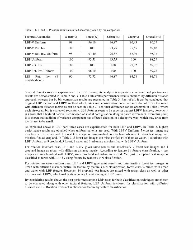
Since different cases are experimented for LBP feature, its analysis is separately conducted and performance results are demonstrated in Table 2 and 3. Table 1 illustrates performance results obtained by diffusion distance approach whereas bin-by-bin comparison results are presented in Table 3. First of all, it can be concluded that original LBP method and LBPV method which takes into consideration local variance do not differ too much with diffusion distance metric as can be seen in Table 2. Yet, their difference can be observed in Table 3 where each histogram bin is evaluated separately. LBP features seem to be superior against LBPV features; however it is known that a textural pattern is composed of spatial configuration along variance differences. From this point, it is shown that addition of variance component has affected decision in a deceptive way, which may arise from the dataset to be small.
As explained above in LBP part, three cases are experimented for both LBP and LBPV. In Table 2, highest performance results are obtained when uniform patterns are used. With LBPV Uniform, 5 crop test image are misclassified as urban and 1 forest test image is misclassified as cropland whereas 4 urban test image are misclassified as cropland. In Table 3, 5 forest test images are misclassified (4 of them as water, 1 as urban) with LBP Uniform, as 9 cropland, 3 forest, 1 water and 1 urban are misclassified with LBPV Uniform.
For rotation invariant case, LBP and LBPV gives same results and misclassify 7 forest test images and 1 cropland image as urban with diffusion distance metric. According to feature by feature classification, 4 test images are misclassified with LBPV, since cropland and urban are mixed. Yet, just 1 cropland test image is classified as forest with LBP by using feature by feature k-NN classification.
For rotation invariant-uniform case, LBP and LBPV give same results and misclassify 8 forest test images as urban with diffusion distance metric. In feature by feature k-NN classification, forest class is mixed with urban and water with LBP feature. However, 14 cropland test images are mixed with urban class as well as other mixtures with LBPV, which makes its accuracy lowest among all LBP cases.
By considering results above, the best performers among LBP cases for both classification techniques are chosen to be evaluated along with other textural features. LBP Uniform is chosen for classification with diffusion distance as LBP Rotation Invariant is chosen for feature by feature classification.
Table 4. Results of k-NN classification
Features\Accuracies Water(%) Forest(%) Urban(%) Crop(%) Overall (%)
GLCM 98 94,80 96,87 76,09 95,85
Gabor 100 100 100 97,82 99,76
HOG 100 100 68,75 84,78 95,85
LBP Rot. Inv. 100 100 100 97,82 99,76
LEP 90 72,72 96,87 84,78 91,71
Edge Orientation 76 72,72 93,75 91,30 90,49
Color Histogram 94 96,10 100 93,48 97,80
Table 5. Results of Diffusion Distance classification
Features\Accuracies Water(%) Forest(%) Urban(%) Crop(%) Overall (%)
HOG 100 100 68,75 84,78 96,83
LBP Uniform 100 100 87,50 100 99,02
LEP 90 71,43 96,87 84,78 91,46
Edge Orientation 74 88,31 93,75 86,95 92,68
Color Histogram 100 96,10 100 100 99,27
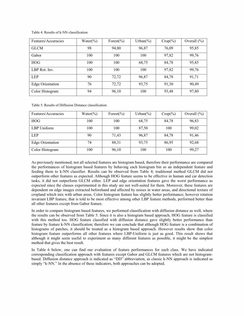
As previously mentioned, not all selected features are histogram based, therefore their performance are compared the performances of histogram based features by behaving each histogram bin as an independent feature and feeding them to k-NN classifier. Results can be observed from Table 4; traditional method GLCM did not outperform other features as expected. Although HOG feature seems to be effective in human and car detection tasks, it did not outperform GLCM either. LEP and edge orientation features gave the worst performance as expected since the classes experimented in this study are not well-suited for them. Moreover, these features are dependent on edge images extracted beforehand and affected by noises in water areas, and directional texture of cropland which mix with urban areas. Color histogram feature has slightly better performance; however rotation invariant LBP feature, that is told to be most effective among other LBP feature methods, performed better than all other features except from Gabor feature.
In order to compare histogram based features, we performed classification with diffusion distance as well, where the results can be observed from Table 5. Since it is also a histogram based approach, HOG feature is classified with this method too. HOG feature classified with diffusion distance gave slightly better performance than feature by feature k-NN classification; therefore we can conclude that although HOG feature is a combination of histograms of patches, it should be treated as a histogram based approach. However results show that color histogram feature outperforms all other features where LBP-Uniform is just as good. This result shows that although it might seem useful to experiment as many different features as possible, it might be the simplest method that gives the best result.
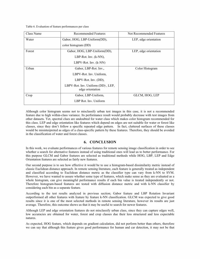
In Table 6 below, one can find our evaluation of feature performances for each class. We have indicated corresponding classification approach with features except Gabor and GLCM features which are not histogram- based. Diffusion distance approach is indicated as “DD” abbreviation, as classic k-NN approach is indicated as simply “k-NN.” In the absence of these indicators, both approaches can be adopted.
Table 6. Evaluation of feature performances per class
Class Name Recommended Features Not Recommended Features
Water Gabor, HOG, LBP-Uniform(DD),
Color Histogram
GLCM, HOG, LEP
Although color histogram seems not to misclassify urban test images in this case, it is not a recommended feature due to high within-class variance. Its performance result would probably decrease with test images from other datasets. Yet, spectral clues are undoubted for water class which makes color histogram recommended for this class. LEP and edge orientation like features which depend on edges are not suitable for water or forest like classes, since they don’t follow a specific repeated edge pattern. In fact, cluttered surfaces of these classes would be misinterpreted as edges of a class-specific pattern by these features. Therefore, they should be avoided in the classification of water and forest classes.
6. CONCLUSION In this work, we evaluate performances of various features for remote sensing image classification in order to see whether a search for alternative features instead of using traditional ones will lead us to better performance. For this purpose GLCM and Gabor features are selected as traditional methods while HOG, LBP, LEP and Edge Orientation features are selected as fairly new features.
Our second purpose is to see how effective it would be to use a histogram-based dissimilarity metric instead of classic Euclidean distance approach. In remote sensing literature, each feature is generally treated as independent and classified according to Euclidean distance metric as the classifier type can vary from k-NN to SVM. However, we have wanted to assure whether some type of features, which make sense as they are evaluated as a whole histogram, can give meaningful performance results if each bin value is treated independently or not. Therefore histogram-based features are tested with diffusion distance metric and with k-NN classifier by considering each bin as a separate feature.
According to the test results analyzed in previous section; Gabor feature and LBP Rotation Invariant outperformed all other features with feature by feature k-NN classification. GLCM was expected to give good results since it is one of the most selected methods in remote sensing literature, however its results are just average. Therefore, this outcome shows us that it may be useful to search for newer features.
Although LEP and edge orientation features do not misclassify urban class, since they can capture edges well, low accuracies are obtained for water, forest and crop classes due their less structured and less expectable natures.
As expected, HOG feature, which depends on gradient calculation, did not perform better than others, therefore we can say that although this feature gives good performance for human and car detection, it may not be that
successful for land use/land cover classification, since remote sensing classes do not generally obey a general structure.
As previously stated, Gabor features gave one of the most successful results with classic k-NN classification. Like GLCM, this feature is traditional too; however its representativeness of texture is much better than GLCM.
Although LBP feature is characteristically used as a whole histogram and was expected to fail with classic k-NN classification approach, the results show otherwise, as its performance is as good as Gabor feature and outperforms LBP performances obtained during histogram comparison.
At histogram based classification with Diffusion Distance, LBP Uniform gave good performance, however best performance is taken from color histogram method. This result points to the fact that although it might be useful to work with complex features; sometimes best results can be obtained from the simplest ones. Though if another test data was used instead of Fethiye, because of variation in colors, this feature may not give the best performance, quite the reverse it would give the worst. Due to high variation of spectral values in different remote sensing data, selection of textural features would be a better choice instead of color-dependent ones.
Although evaluation of features is proceeded with 7 features in this work, many other features can be implemented as well. Also using SVM classifier instead of k-NN might change the results widely.
During comparison of classification techniques, other histogram-based dissimilarity metrics like Kullback- Leibler distance should also be tested for further analysis.
Dataset used for this experiment may be broadened for future experiments by adding other classes with specific textures and by adding other images with varying spectral values. In this way, more general outcomes can be derived from experiments.
ACKNOWLEDGEMENT
REFERENCES
[1] Haralick, R. M., Shanmugam K. and Dinstein, I., "Textural features for image classification," IEEE Transactions on Systems, Man, and Cybernetics SMC-3, 610-621 (1973).
[2] Vatsavai, R.R., Cheriyadat, A. and Gleason, S., "Unsupervised semantic labeling framework for identification of complex facilities in high-resolution remote sensing images," Data Mining Workshops (ICDMW), 2010 IEEE International Conference, 273-280 (2010).
[3] Tobin,K. W., Bhaduri, B. L. and Bright, E. A., "Large-scale geospatial indexing for image-based retrieval and analysis," Proc. International Symposium on Visual Computing. 69121 Heidelberg, Germany: LNCS 3804, Springer Verlag, (2005).
[4] Freeman, W. and Adelson, E., "The design and use of steerable filters," Pattern Analysis and Machine Intelligence, IEEE Transactions, vol. 13, 891-906 (1991).
[5] Dalal, N. and Triggs, B., "Histograms of Oriented gradients for human detection," IEEE Computer Society Conference on Computer Vision and Pattern Recognition (CVPR'05), vol. 1, 886-893 (2005).
[6] Ling, H. and Okada, K., "Diffusion distance for histogram comparison," Computer Vision and Pattern Recognition, 2006 IEEE Computer Society Conference, vol.1, 246-253 (2006).
[7] Huang, Y., Yue, A. and Wei, S., "Texture feature extraction for land-cover classification of remote sensing data in land consolidation district using semi-variogram analysis," W. Trans. on Comp. vol. 7, 857-866 (2008).
[8] Yang, Y. and Newsam, S., "Comparing SIFT descriptors and Gabor texture features for classification of remote sensed imagery," Image Processing, 2008. ICIP 2008. 15th IEEE International Conference, 1852-1855 (2008).
[9] Bandzi, P., Oravec, M. and Pavlovicova, J., "New statistics for texture classification based on Gabor filters," Radioengineering, vol. 16, 133-136 (2007).
[10] Grigorescu, S., Petkov, N. and Kruizinga, P., "Comparison of texture features based on Gabor filters," IEEE Transactions on Image Processing, vol. 11, 1160-1167 (2002).
[11] Daugman, J. G., "Uncertainty relation for resolution in space, spatial frequency, and orientation optimized by two-dimensional visual cortical filters," Journal of the Optical Society of America A, 2(7), 1160-1169 (1985).
[12] Gleason, J., Nefian, A., Bouyssounousse, X., Fong, T. and Bebis, G., "Vehicle detection from aerial imagery," IEEE International Conference on Robotics and Automation (ICRA11), Shanghai, China (2011).
[13] Tuermer, S., Leitloff, J., Reinartz, P. and Stilla, U., "Evaluation of selected features for car detection in aerial images," ISPRS Hannover Workshop, High-Resolution Earth Imaging for Geospatial Information, (2011).
[14] Kullback, S. and Leibler, R. A., "On information and sufficiency," Annals of Mathematical Statistics 22 (1), 79-86 (1951).
[15] Guo, Z., Zhang, L. and Zhang, D., "Rotation invariant texture classification using LBP Variance (LBPV) with global matching," Pattern Recognition, vol. 43, 706-719 (2010).
[16] Ojala, T., Pietikäinen, M. and Mäenpää, T., "Gray scale and rotation invariant texture classification with local binary patterns," Computer Vision, ECCV 2000 Proceedings, Lecture Notes in Computer Science 1842, Springer, 404-420 (2000).
[17] Ojala, T., Pietikäinen, M. and Mäenpää, T., "A generalized local binary pattern operator for multi resolution gray scale and rotation invariant texture classification," Advances in Pattern Recognition, ICAPR 2001 Proceedings, Lecture Notes in Computer Science 2013, Springer, 397-406 (2001).
[18] Canny, J., "A computational approach to edge detection," IEEE Trans. Pattern Analysis and Machine Intelligence, 8(6), 679-698 (1986).
[19] Otsu, N., "A Threshold selection method from gray-level histograms," IEEE Transactions on Systems, Man, and Cybernetics, Vol. 9, 62-66 (1979).
[20] Duda, R. O., Hart, P. E. and Stork, D. G., "Pattern classification", New York: John Wiley & Sons, 202- 214 (2001).
[21] Chang, T. and Kuo, C. C. J., "Texture analysis and classification with tree-structured wavelet transform," IEEE Transactions on Image Processing, 2 (4), 429-441 (1993).
[22] Laine, A. and Fan, J., "Texture classification by wavelet packet signatures," IEEE Transactions on Pattern Analysis and Machine Intelligence, 15 (11), 1186-1191 (1993).
[23] Ojala, T., Pietikäinen, M. and Harwood, D., "A comparative study of texture measures with classification based on featured distributions," Pattern Recognition, 29(1), 51-59 (1996).