Evaluation of the effects of aggregate gradation and ...

Graduate Theses, Dissertations, and Problem Reports

2013

Evaluation of the effects of aggregate gradation and compaction Evaluation of the effects of aggregate gradation and compaction

effort on the voids in mineral aggregate in asphalt concrete effort on the voids in mineral aggregate in asphalt concrete

Logan Bessette

Follow this and additional works at: https://researchrepository.wvu.edu/etd

Recommended Citation Recommended Citation Bessette, Logan, "Evaluation of the effects of aggregate gradation and compaction effort on the voids in mineral aggregate in asphalt concrete" (2013). Graduate Theses, Dissertations, and Problem Reports. 7301. https://researchrepository.wvu.edu/etd/7301

This Thesis is protected by copyright and/or related rights. It has been brought to you by the The Research Repository @ WVU with permission from the rights-holder(s). You are free to use this Thesis in any way that is permitted by the copyright and related rights legislation that applies to your use. For other uses you must obtain permission from the rights-holder(s) directly, unless additional rights are indicated by a Creative Commons license in the record and/ or on the work itself. This Thesis has been accepted for inclusion in WVU Graduate Theses, Dissertations, and Problem Reports collection by an authorized administrator of The Research Repository @ WVU. For more information, please contact [email protected].

https://researchrepository.wvu.edu/

https://researchrepository.wvu.edu/

https://researchrepository.wvu.edu/etd

https://researchrepository.wvu.edu/etd?utm_source=researchrepository.wvu.edu%2Fetd%2F7301&utm_medium=PDF&utm_campaign=PDFCoverPages

https://researchrepository.wvu.edu/etd/7301?utm_source=researchrepository.wvu.edu%2Fetd%2F7301&utm_medium=PDF&utm_campaign=PDFCoverPages

mailto:[email protected]

EVALUATION OF THE EFFECTS OF AGGREGATE GRADATION AND

COMPACTION EFFORT ON THE VOIDS IN MINERAL AGGREGATE IN ASPHALT

CONCRETE

Logan Bessette

Thesis submitted to the

Benjamin M. Statler College of Engineering and Mineral Resources

at West Virginia University

in partial fulfillment of the requirements

for the degree of

Master of Science

in

Civil Engineering

Dr. John P. Zaniewski, Chair

Dr. John Quaranta

Dr. Avinash Unnikrishnan

Department of Civil and Environmental Engineering

Morgantown, West Virginia

2013

Keywords: Voids in Mineral Aggregate (VMA), Fracture Energy, Compaction Effort

All rights reserved

INFORMATION TO ALL USERSThe quality of this reproduction is dependent upon the quality of the copy submitted.

In the unlikely event that the author did not send a complete manuscriptand there are missing pages, these will be noted. Also, if material had to be removed,

a note will indicate the deletion.

Microform Edition © ProQuest LLC.All rights reserved. This work is protected against

unauthorized copying under Title 17, United States Code

ProQuest LLC.789 East Eisenhower Parkway

P.O. Box 1346Ann Arbor, MI 48106 - 1346

UMI 1549729Published by ProQuest LLC (2013). Copyright in the Dissertation held by the Author.

UMI Number: 1549729

i

ABSTRACT

EVALUATION OF THE EFFECT OF AGGREGATE GRADATION AND COMPACTION EFFORT ON THE

VOIDS IN MINERAL AGGREGATE IN ASPHALT CONCRETE

Logan Bessette

Asphalt concrete should resist short-term rutting, provide resistance to thermal cracking,

and maintain structural integrity through the design life of the structure. Balancing these factors

is achieved by ensuring adequate asphalt binder in a strong aggregate structure. The design

asphalt content is decreased by applying additional compaction effort in the form of increased

gyrations in the Superpave Gyrator Compactor. The mixes that undergo increased compaction

effort present decreased fatigue life, although they resist short-term rutting. Mixes that undergo

less compaction effort contain more binder and have long fatigue lives, although they are

susceptible to rutting.

Two hypotheses were tested to determine the effects of compaction effort, and gradation

on the voids in mineral aggregate. Three gradations were tested to simulate the range of

aggregate gradations allowed within the West Virginia Department of Highways control points

for 9.5mm asphalt concrete at compaction levels of 80, and 100 gyrations. The reduction in the

number of design gyrations for asphalt concretes in West Virginia does not create significant

differences in the design parameter, voids in mineral aggregate (VMA). At a given compaction

level, moving away from the maximum density line, either coarse- or fine-graded, creates

statistically different VMA.

Additionally, the bulk specific gravity samples were tested for indirect tensile (IDT)

strength, and fracture energy. The 80 gyration mixes presented higher IDT strength than the 100

gyration mixes. Mixes with high compaction slopes presented the lowest IDT strength. Using the

load-deflection curves from the IDT test, the fracture energy was calculated. The 80 gyration

mixes had fracture energy 32% greater than the 100 gyration mixes, indicating an increased

fatigue life. The coarse graded mix has the largest increase in fracture energy when reducing

compaction effort, although it had the lowest IDT strength.

ii

TABLE OF CONTENTS

Abstract ............................................................................................................................................ i

List of Figures ................................................................................................................................... v

List of Tables ................................................................................................................................... vi

Chapter 1 Introduction ................................................................................................................... 1

Background .................................................................................................................................. 1

Problem Statement ..................................................................................................................... 2

Objective ..................................................................................................................................... 2

Scope and Limitations ................................................................................................................. 2

Organization of Thesis ................................................................................................................. 2

Chapter 2 Literature Review ........................................................................................................... 4

Introduction................................................................................................................................. 4

Asphalt Concrete Mixture Design ............................................................................................... 4

Marshall ................................................................................................................................... 4

Superpave ................................................................................................................................ 5

Volumetric Requirements ........................................................................................................... 7

Volumetric Properties ................................................................................................................. 9

Voids in Total Mix .................................................................................................................... 9

Voids Filled with Asphalt ......................................................................................................... 9

Voids in Mineral Aggregate ..................................................................................................... 9

Definition ................................................................................................................................. 9

Determination ....................................................................................................................... 10

History .................................................................................................................................... 10

Factors affecting VMA ........................................................................................................... 12

Effect of VMA on Asphalt Concrete Performance .................................................................... 14

Compaction Effort ..................................................................................................................... 16

Locking Point ............................................................................................................................. 16

Compaction Slope (k) ................................................................................................................ 17

Indirect Tensile Strength ........................................................................................................... 18

iii

Film Thickness ........................................................................................................................... 20

Aggregate Surface Area ......................................................................................................... 20

Summary of Literature Review .................................................................................................. 25

Chapter 3 Research Methodology ................................................................................................ 27

Introduction............................................................................................................................... 27

Experiment Design .................................................................................................................... 27

Gradations ................................................................................................................................. 28

Sample Creation ........................................................................................................................ 30

Analysis ...................................................................................................................................... 30

IDT Strength Testing .................................................................................................................. 31

Fracture Energy ......................................................................................................................... 31

Locking Point and Compaction Slope ........................................................................................ 31

Statistical Analysis ..................................................................................................................... 31

ANOVA ................................................................................................................................... 31

Tukey Kramer Honest Significant Difference (HSD) .................................................................. 32

Linear Regression ...................................................................................................................... 32

Summary of Research Methodology ......................................................................................... 33

Chapter 4 Results and Analysis ..................................................................................................... 34

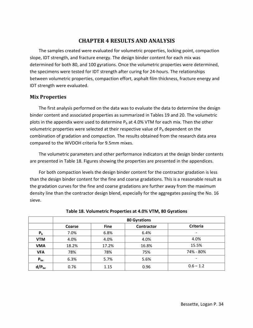
Mix Properties ........................................................................................................................... 34

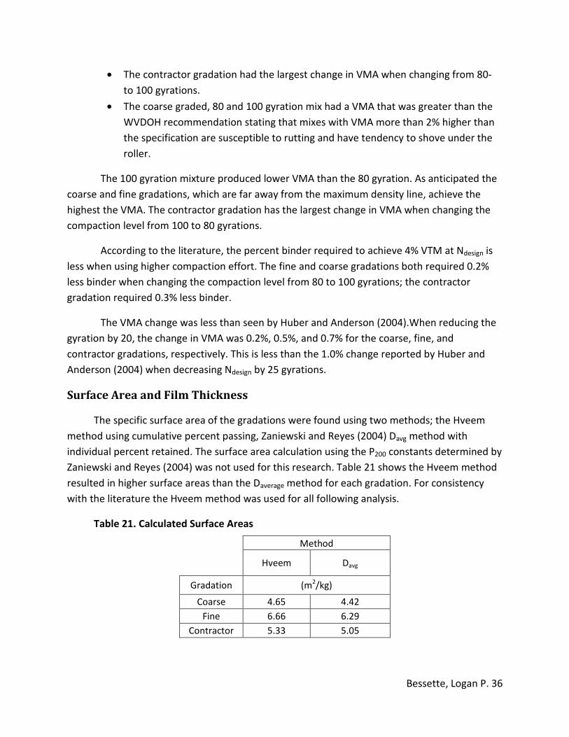
Surface Area and Film Thickness ............................................................................................... 36

Film Thickness ........................................................................................................................... 37

Indirect Tensile Strength ........................................................................................................... 37

Fracture Energy ......................................................................................................................... 39

Locking Point ............................................................................................................................. 42

Comparison of IDT Strength and Compaction Effort............................................................. 45

ANOVA Summary ...................................................................................................................... 47

Comparison of Gyrations ....................................................................................................... 47

Comparison of Gradation ...................................................................................................... 50

Summary of Results ................................................................................................................... 52

iv

Chapter 5 Conclusion and Recommendations.............................................................................. 53

Recommendations for Further Research .................................................................................. 54

References .................................................................................................................................... 55

Appendix ....................................................................................................................................... 59

v

LIST OF FIGURES

Figure 1.Rut Rate vs. Design VMA................................................................................................. 15

Figure 2.Rut Rate vs. Design VMA FM300 ...................................................................................... 15

Figure 3. Fatigue life vs. Design VMA ............................................................................................ 16

Figure 4. IDT strength test, prior to failure, and failed specimen ................................................ 18

Figure 5. Rut Depth vs. IDT Strength............................................................................................. 19

Figure 6. IDT Fracture Energy vs. Fatigue Life (Cycles) ................................................................. 19

Figure 7. Air Permeability Apparatus ............................................................................................ 23

Figure 8. Surface Area vs FM300 .................................................................................................... 24

Figure 9. Surface Area vs. P75 ........................................................................................................ 24

Figure 10. 9.5mm Aggregate Gradations ...................................................................................... 29

Figure 11. Calculated Surface Area, Davg vs. Hveem ..................................................................... 37

Figure 12. Relationship between IDT strength and film thickness at 80 gyrations ...................... 38

Figure 13. Relationship between IDT strength and film thickness at 100 gyrations .................... 38

Figure 14. Example Fracture Energy from IDT Load Diagram ....................................................... 39

Figure 15. Fracture Energy vs. IDT Strength ................................................................................. 41

Figure 16. Compaction slope vs. Film thickness ........................................................................... 44

Figure 17. Dust-to-film thickness ratio vs. dust-to-effective binder ratio .................................... 45

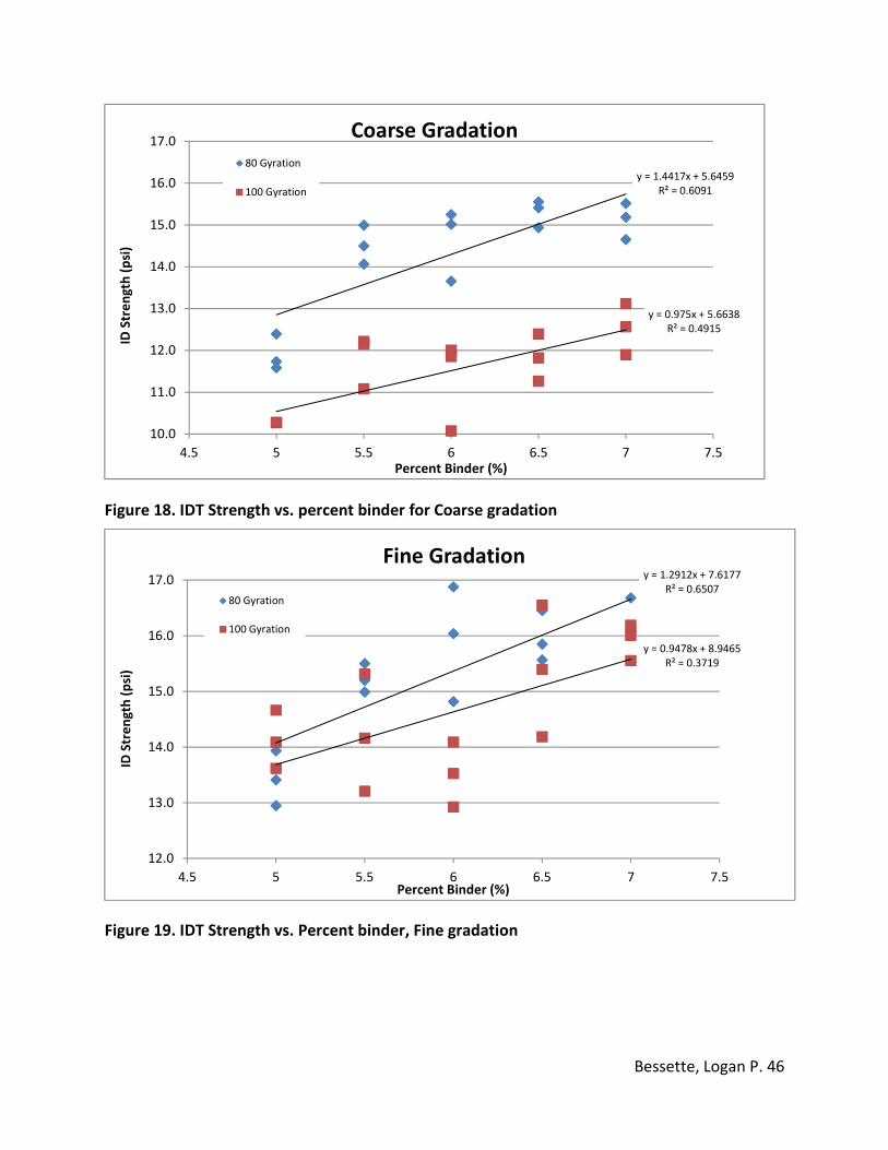
Figure 18. IDT Strength vs. percent binder for Coarse gradation ................................................. 46

Figure 19. IDT Strength vs. Percent binder, Fine gradation .......................................................... 46

Figure 20. IDT Strength vs. Percent binder, Contractor gradation ............................................... 47

Figure 21. Coarse Gradation, VTM (%) vs. Percent Binder ........................................................... 60

Figure 22. Fine Gradation, VTM (%) vs. Percent Binder ............................................................... 60

Figure 23. Contractor Gradation, VTM(%) vs. Percent Binder ...................................................... 60

Figure 24. Coarse Gradation, VFA vs. Percent Binder .................................................................. 61

Figure 25. Fine Gradation, VFA vs. Percent Binder ....................................................................... 61

Figure 26. Contractor Gradation, VFA vs. Percent Binder ............................................................ 61

Figure 27. Coarse Gradation, VMA vs. Percent Binder ................................................................. 62

Figure 28. Fine Gradation, VMA vs. Percent Binder ..................................................................... 62

Figure 29. Contractor Gradation, VMA vs. Percent Binder........................................................... 63

vi

LIST OF TABLES

Table 1. 1948 Corp of Engineers Limiting Values ........................................................................... 5

Table 2. AASHTO Superpave Gyrator Compaction Effort ............................................................... 6

Table 3. WVDOH Gyratory Compaction Levels ............................................................................... 7

Table 4. WVDOH Marshall Method Volumetric Criteria ................................................................. 7

Table 5. West Virginia Marshall Method VMA Criteria .................................................................. 8

Table 6. WVDOH Superpave Mix Design Criteria ........................................................................... 8

Table 7. WVDOH Superpave Method VMA and VFA Criteria ........................................................ 8

Table 8. Comparison of VMA for Marshall and Superpave .......................................................... 11

Table 9. Comparison of VFA for Marshall and Superpave ............................................................ 12

Table 10. Factors affecting VMA ................................................................................................... 13

Table 11. VMA related to distance from MDL .............................................................................. 13

Table 12. Gradations used by Huber & Shuler.............................................................................. 14

Table 13. Example of Locking Point from SGC height output ....................................................... 17

Table 14. Surface area for one gram of uniform sand .................................................................. 21

Table 15. Surface Area Factors, based on Percent Passing .......................................................... 22

Table 16. Specific area for material less than 75 microns ............................................................ 23

Table 17. Testing matrix ................................................................................................................ 28

Table 18. Volumetric Properties at 4.0% VTM, 80 Gyrations ....................................................... 34

Table 19. Volumetric Parameters at 4% VTM, 100 Gyrations ...................................................... 35

Table 20. Mix Properties at Design Binder Content* ................................................................... 35

Table 21. Calculated Surface Areas ............................................................................................... 36

Table 22. IDT Strength and Fracture Energy ................................................................................. 42

Table 23. Gyrations to achieve locking point ................................................................................ 43

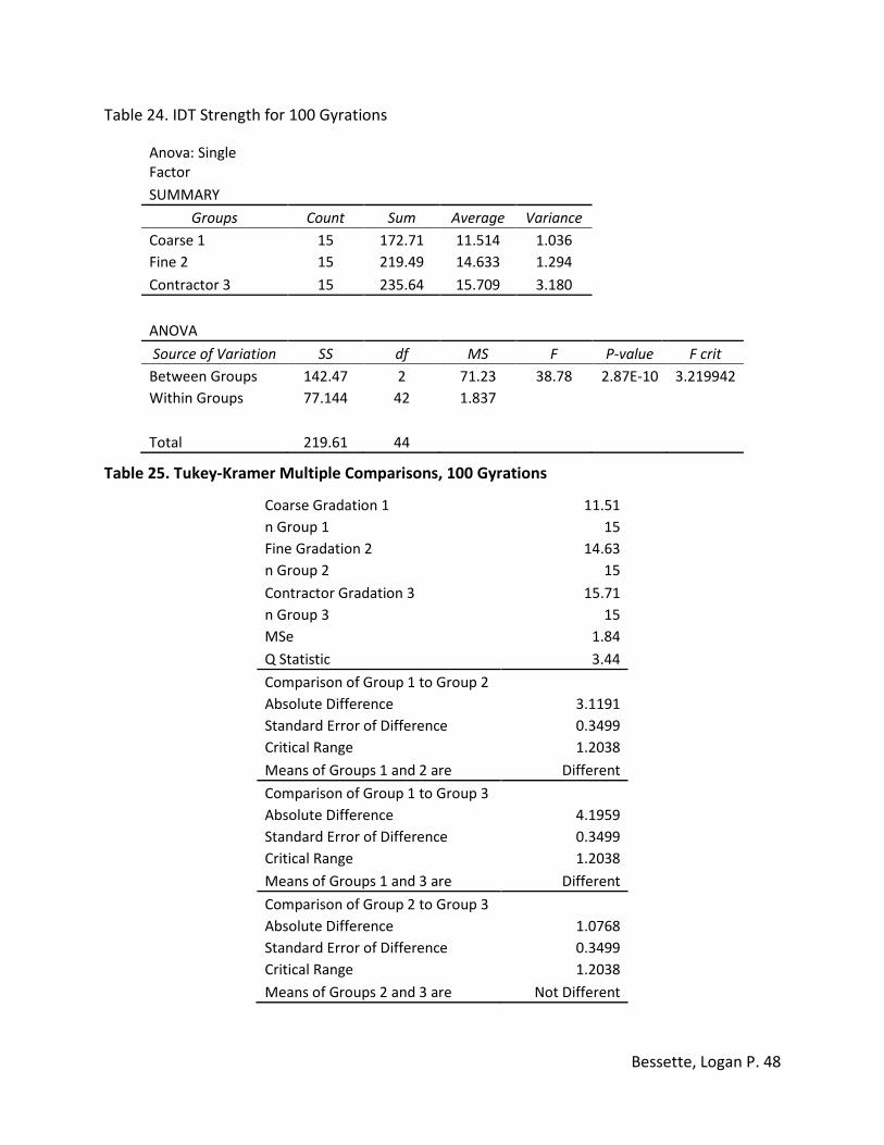
Table 24. IDT Strength for 100 Gyrations ..................................................................................... 48

Table 25. Tukey-Kramer Multiple Comparisons, 100 Gyrations ................................................... 48

Table 26. IDT Strength for 80 Gyrations ....................................................................................... 49

Table 27. Tukey-Kramer Multiple Comparisons 80 Gyrations ...................................................... 49

Table 28. ANOVA Table for Gyrations ........................................................................................... 50

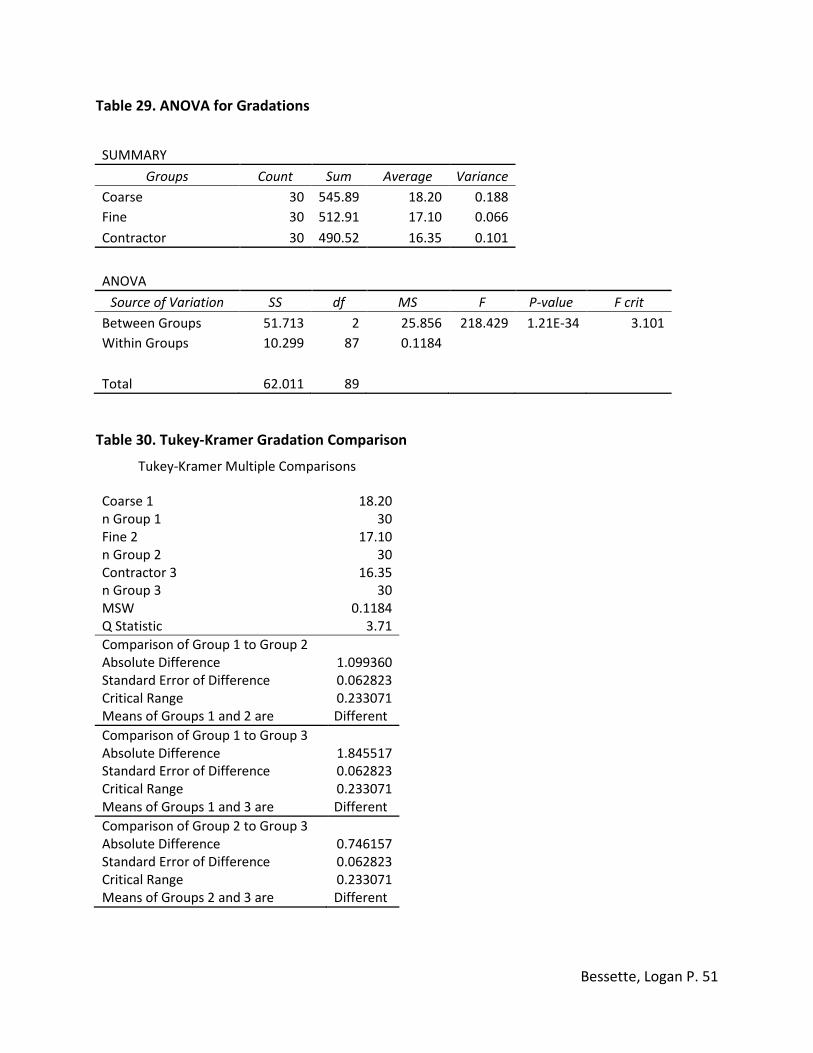
Table 29. ANOVA for Gradations .................................................................................................. 51

Table 30. Tukey-Kramer Gradation Comparison .......................................................................... 51

Bessette, Logan P. 1

CHAPTER 1 INTRODUCTION

Background

As of 2005 there were approximately 4 million miles of roads in the United States, 2.4

million miles of these roads are covered with asphalt concrete (Roberts et al., 2009). The

abundance of both freight and commuter vehicles on these roads means that it is important

that asphalt pavements be designed to provide both long-term durability, and high

performance when subjected to environmental and load induced stresses.

Asphalt concrete is comprised of three primary components, asphalt binder, aggregate,

and air. Asphalt binder is a bituminous material that is largely produced through petroleum

distillation. The material has viscous, elastic, and plastic behavior dependent on temperature.

Asphalt binder is heated, and used to coat aggregate particles and bind them together. Asphalt

binder can be produced to create desired performance characteristics based on the expected

temperature range of the pavement.

Aggregates comprise approximately 95% of the asphalt concrete by mass (85% by volume).

Depending on location, the aggregates used in asphalt concrete vary largely but all are

expected to exhibit the same desirable characteristics of mechanical strength, durability,

chemical durability, and desirable surface characteristics (Roberts et al., 2009). Aggregates

range from natural products collected in river beds, to materials that have been blasted from

quarries and mechanically crushed to create the desired qualities and size. In addition to the

origin of the aggregates, they are also categorized according to the size of the particles to

create design gradations for the aggregate structure in the asphalt concrete.

Air is the final constituent in asphalt concrete. Air voids within the mixture allow space for

the thermal expansion and contraction of the asphalt binder. The mixture is mechanically

compacted. After compaction, the mixture cools, and the final product is a material that can be

subjected to high loads and many repetitions such as those on the interstate highway system.

In 1943 Bruce Marshall and the Army Corps of Engineers worked to create a portable

apparatus to test asphalt for airfield pavements. Through development and modifications it

would become known as the Marshall Design method. During the 1980’s, Congress outlined a

plan to develop the United States transportation network through improvements to roads and

highways. As a product of the Strategic Highway Research Program (SHRP), the Superpave

design method was developed. These two design methods are now the most common methods

in the United States and are related through the use of extensive volumetric analysis to create a

quality pavement (Roberts et al., 2009). The West Virginia Division of Highways (WVDOH)

currently uses both the Marshall and Superpave methods.


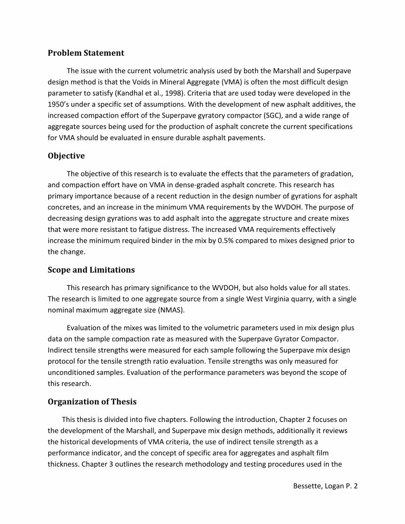
Problem Statement

The issue with the current volumetric analysis used by both the Marshall and Superpave

design method is that the Voids in Mineral Aggregate (VMA) is often the most difficult design

parameter to satisfy (Kandhal et al., 1998). Criteria that are used today were developed in the

1950’s under a specific set of assumptions. With the development of new asphalt additives, the

increased compaction effort of the Superpave gyratory compactor (SGC), and a wide range of

aggregate sources being used for the production of asphalt concrete the current specifications

for VMA should be evaluated in ensure durable asphalt pavements.

Objective

The objective of this research is to evaluate the effects that the parameters of gradation,

and compaction effort have on VMA in dense-graded asphalt concrete. This research has

primary importance because of a recent reduction in the design number of gyrations for asphalt

concretes, and an increase in the minimum VMA requirements by the WVDOH. The purpose of

decreasing design gyrations was to add asphalt into the aggregate structure and create mixes

that were more resistant to fatigue distress. The increased VMA requirements effectively

increase the minimum required binder in the mix by 0.5% compared to mixes designed prior to

the change.

Scope and Limitations

This research has primary significance to the WVDOH, but also holds value for all states.

The research is limited to one aggregate source from a single West Virginia quarry, with a single

nominal maximum aggregate size (NMAS).

Evaluation of the mixes was limited to the volumetric parameters used in mix design plus

data on the sample compaction rate as measured with the Superpave Gyrator Compactor.

Indirect tensile strengths were measured for each sample following the Superpave mix design

protocol for the tensile strength ratio evaluation. Tensile strengths was only measured for

unconditioned samples. Evaluation of the performance parameters was beyond the scope of

this research.

Organization of Thesis

This thesis is divided into five chapters. Following the introduction, Chapter 2 focuses on

the development of the Marshall, and Superpave mix design methods, additionally it reviews

the historical developments of VMA criteria, the use of indirect tensile strength as a

performance indicator, and the concept of specific area for aggregates and asphalt film

thickness. Chapter 3 outlines the research methodology and testing procedures used in the


laboratory. Chapter 4 contains the results, and the analysis of the results from laboratory

testing. Chapter 5 presents conclusions from the testing conducted and proposes

recommendations to design economical and high performance asphalt pavements. The

appendix contains all results from laboratory testing and mathematical equations


CHAPTER 2 LITERATURE REVIEW

Introduction

The research presented in this thesis builds upon the volumetric properties, and concepts

that are well established in both academic literature, and literature from the asphalt paving

industry. The use of volumetric criteria by the WVDOH is based around the recommendations

of American Association of State Highway and Transportation Officials (AASHTO) and the

Asphalt Institute (TAI) for the requirements regarding volumetric properties for Superpave and

Marshall methods, respectively.

Prior to the introduction of the Superpave in the early 1990’s most states designed asphalt

pavements with either the Marshall or Hveem Method. In 1984, approximately 25% of the

states used a variation of the Hveem method, and the remainder used a variation of the

Marshall Design method (Asphalt Institute, 2007). With the introduction of the Superpave

design method, the primary methods for asphalt pavement design are currently the Marshall

and Superpave methods (FHWA, 1995) and are the focus of this literature review.

Asphalt Concrete Mixture Design

Marshall

The Marshall mix design method was conceived by Bruce Marshall of the Mississippi

Highway Department. Marshall’s method was researched by the Corps of Engineers (COE) and

in 1943 it was adopted for the design of airfield pavements (Roberts et al., 2009). The COE

manipulated the Marshall hammer to apply a variety of compaction efforts to simulate the

construction of asphalt pavements in the field. The compaction effort was varied by changing

the number of blows from the hammer, the weight of the hammer, and the distance the

hammer fell. The final Marshall hammer produced by the COE was a portable apparatus, with a

10-lb hammer falling 18 inches, a 3-7/8’’ inches diameter foot, a 4-inch diameter mold, and a

standard compaction effort of 35 blows per side. With an increase of aircraft size and weight in

the 1950’s the laboratory compaction efforts were increased to 50 blows on each side of the

specimen (Roberts et al., 2009). In May 1948, the COE presented the limiting values of testing


properties for asphalt concretes designed with the Marshall method, classification was either

“Brittle”, “Satisfactory,” or “Plastic,” as presented in Table 1. There were no requirements for

VMA in the 1948 COE design criteria (USCOE, 1948). However, there were voids filled with

asphalt (VFA) criterion. The WVDOH currently uses 50 and 75 blows for the design of Marshall

mixes for medium and heavy traffic, respectively (WVDOH, MP 401.02.22)

Table 1. 1948 Corp of Engineers Limiting Values

Test Property Brittle Satisfactory Plastic

Flow Value No Lower Limit 20 or less More than 20

Percent Air Voids More than 5 5-3 Less than 3

Percent Voids

filled with Asphalt Less than 70 75 to 85 More than 85

Superpave

In 1987, Congress authorized a five-year research program, SHRP, to combat the

deterioration of the United States highways and to improve safety, performance and overall

durability of highway infrastructure (Roberts et al., 2009). The research initiative was

undertaken by industry, academia, and government agencies and focus on asphalt pavements,

concrete structures, maintenance and work zone safety, and long term pavement performance

studies. The scope of this literature review follows the developments only regarding asphalt

pavements, and primarily the Superpave design method.

The Superpave design method was developed as a procedure to better predict asphalt

concrete field performance (Christensen and Bonaquist, 2006). A major outcome of SHRP was

the development of the Superpave Gyrator Compactor (SGC). The SGC uses a constant vertical

stress of 600 kPa, an internal compaction angle of 1.25°, a gyration speed of 30 gyrations per

minute and number of gyrations. The first three parameters are kept constant and the number

of gyrations is varied for different mix types and applications. Table 2 presents the AASHTO

compaction recommendation and Table 3 presents the compaction levels used by the WVDOH

(WVDOH, MP 401.02.28)


The size of the specimen produced was also increased from 4 inches in diameter under

Marshall to 150 mm in diameter under Superpave. The rationale behind this was to allow

larger aggregates to be used without causing compaction problems (Roberts et. al. 2009),

although there was a six inch Marshall mold to create base layer specimens.

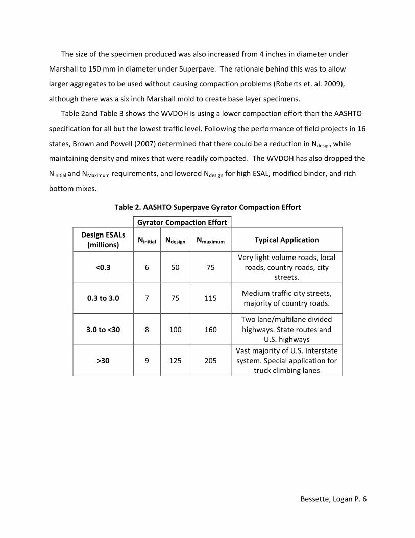
Table 2and Table 3 shows the WVDOH is using a lower compaction effort than the AASHTO

specification for all but the lowest traffic level. Following the performance of field projects in 16

states, Brown and Powell (2007) determined that there could be a reduction in Ndesign while

maintaining density and mixes that were readily compacted. The WVDOH has also dropped the

Ninitial and NMaximum requirements, and lowered Ndesign for high ESAL, modified binder, and rich

bottom mixes.

Table 2. AASHTO Superpave Gyrator Compaction Effort

Gyrator Compaction Effort

Design ESALs

(millions) Ninitial Ndesign Nmaximum Typical Application

<0.3 6 50 75

Very light volume roads, local

roads, country roads, city

streets.

0.3 to 3.0 7 75 115 Medium traffic city streets,

majority of country roads.

3.0 to <30 8 100 160

Two lane/multilane divided

highways. State routes and

U.S. highways

>30 9 125 205

Vast majority of U.S. Interstate

system. Special application for

truck climbing lanes


Table 3. WVDOH Gyratory Compaction Levels

Compaction Parameters

Gyration Level-1 Gyration Level-2

20 Year

Projected design

ESALs (millions)

Ndesign for Binder <

PG 76-XX

Ndesign for Binders ≥ PG

76-XX or Mixes Placed

Below Top Two Lifts

< 0.3 50 50

0.3 to < 3.0 65 65

3.0 to < 30 80 65

≥ 30 100 80

Volumetric Requirements

The current design criteria for Marshall in West Virginia follow the recommendations

from both the American Association of State and Highway Transportation Officials (AASHTO).

The Superpave gyration levels are based on recommendation by the National Cooperative

Highway Research Program (NCHRP). Table 4 and Table 5 present the current criteria in West

Virginia for asphalt concrete designed under the Marshall Method:

Table 4. WVDOH Marshall Method Volumetric Criteria

Design Criteria Medium Traffic

Design1

Heavy

Traffic

Design

Base-I

Design 2

Compaction, number of blows 50 75 112

Stability (Newtons) (minimum) 5,300 8,000 13,300

Flow (0.25 mm)3 8 to 14 8 to 14 8 to 14

Percent Air Voids 4.0 4.0 4.0

Percent Voids Filled with Asphalt 4 65 to 80 65 to 78 64 to 73

Fines-to-Asphalt Ratio 0.6 to 1.2

Note1: All Wearing-III mixes shall be designed as a 50 blow mix;

Note2.All Base I mixes will be designed and tested with 112 blows and 6 inch specimen;

Note3: When using a recording chart to determine the flow value, the flow is normally

read at the point of maximum stability just before it begins to decrease. This approach

works fine when the stability plot is a reasonably smooth rounded curve. Some mixes

comprised of very angular aggregates may exhibit aggregate interlocking which causes

the plot to produce a flat line at the peak stability before it begins to drop. This type of


plot is often difficult to interpret, and sometimes the stability will even start increasing

again after the initial flat line peak. When such a stability plot occurs, the stability and

flow value shall be read at the initial point of peak stability.

Note4: Wearing I Heavy design will have a VFA range of 73 to 78 percent, a Wearing III

mix shall have a VFA range of 75 to 81 percent.

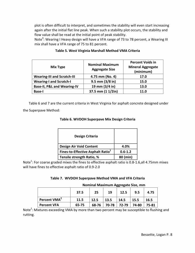
Table 5. West Virginia Marshall Method VMA Criteria

Mix Type Nominal Maximum

Aggregate Size

Percent Voids in

Mineral Aggregate

(minimum)

Wearing-III and Scratch-III 4.75 mm (No. 4) 17.0

Wearing-I and Scratch-I 9.5 mm (3/8 in) 15.0

Base-II, P&L and Wearing-IV 19 mm (3/4 in) 13.0

Base-I 37.5 mm (1 1/2in) 11.0

Table 6 and 7 are the current criteria in West Virginia for asphalt concrete designed under

the Superpave Method:

Table 6. WVDOH Superpave Mix Design Criteria

Design Criteria

Design Air Void Content 4.0%

Fines-to-Effective Asphalt Ratio1

0.6-1.2

Tensile strength Ratio, % 80 (min)

Note1: For coarse graded mixes the fines to effective asphalt ratio is 0.8-1.6,all 4.75mm mixes

will have fines to effective asphalt ratio of 0.9-2.0

Table 7. WVDOH Superpave Method VMA and VFA Criteria

Nominal Maximum Aggregate Size, mm

37.5 25 19 12.5 9.5 4.75

Percent VMA2 11.5 12.5 13.5 14.5 15.5 16.5

Percent VFA 65-75 68-76 70-78 72-79 74-80 75-81

Note2: Mixtures exceeding VMA by more than two percent may be susceptible to flushing and

rutting.


The minimum VMA criteria for the Superpave method was increased by 0.5% in 2011

along with a reduction compaction effort (WVDOH, MP 402.22.28) as recommended by Brown

and Powell (2007).

Volumetric Properties

Voids in Total Mix

Voids in total mix (VTM) is the volume of all pockets of air between the asphalt coated

aggregate particles in a compacted asphalt concrete. VTM is expressed as a percentage of the

bulk volume of the mixture (Roberts et al., 2009). The design VTM is 4% for laboratory

specimens, although they are often compacted to a level less than this in the field to allow for

densification under loading. VTM is calculated using the maximum and bulk specific gravities in

Equation 1

�� = 100 �1 − �� 1

Where:

VTM= Voids in total Mix (%);

Gmb=Bulk specific gravity of compacted asphalt specimen; and

Gmm=Maximum theoretical specific gravity of loose asphalt mixture.

The concept of using VTM was to ensure that there was adequate air voids to allow

space for the expansion and contraction of asphalt binder (Roberts et al., 2009). The presence

of adequate air voids would decrease the likelihood of rutting. Volumetric analysis based on the

principle that not all of the asphalt is within the matrix of aggregate, some of the asphalt is

absorbed into the surface voids of the aggregate particles, thus decreasing the total effective

volume of asphalt in the mixture.

Voids Filled with Asphalt

Voids filled with asphalt (VFA) are the percentage of the VMA, in volume, that are filled

with asphalt. VFA is calculated in Equation 2

� � = 100 �� − �� 2

Voids in Mineral Aggregate

Definition

The Asphalt institute (1962) definition of voids in the mineral aggregate is:


“VMA consists of the intergranular void spaces between the particles of aggregate in a

compacted mixture. It is the bulk volume of the compacted paving mixture minus the

volume of the aggregate determined from its bulk specific gravity, or the volume of

effective asphalt content plus volume of air voids.”

VMA is expressed as a percentage of the bulk volume of the compacted asphalt

concrete specimen. The volume of effective asphalt is the amount of asphalt that is not

absorbed into the pores of the aggregate particle during mixing, conditioning and compacting.

The effective asphalt creates a film that surrounds the aggregate particles.

Determination

VMA is calculated using Equation 3,

�� = 100 − �� 3

Where:

VMA= Voids in the mineral aggregate;

Gmb= Bulk specific gravity of compacted asphalt specimen;

Ps= Percent stone in the mixture; and

Gsb= Bulk specific gravity of the aggregate.

McLeod (1959) emphasized the importance of using the bulk specific gravity of the

aggregate when calculating VMA. If apparent specific gravity was used the total volume of

surface pores of the aggregate would be included. If the effective specific gravity was used then

the volume of the voids within the aggregate particle filled with binder are included. The use of

bulk specific gravity removes the voids within the aggregate particle regardless of whether or

not they are filled with binder. McLeod numerically demonstrated that VTM and VMA

calculations are incorrect if bulk specific gravity is not used.

The VMA requirement proposed by McLeod (1959) is under the assumptions that the

bulk specific gravity of the aggregate is 2.65, and the binder specific gravity is 1.01. However,

Hinrichsen and Heggen (1996) found that the calculated values of VMA are valid for aggregate

bulk specific gravities between 2.50 and 2.80, and adjustment can be made for aggregates with

specific gravity outside this range.

History

During the early development of mix design procedures, between approximately 1901

through 1905, there were two approaches to determine the design asphalt content (Hudson

and Davis, 1965).The first method, coming from Warren emphasized the minimizing of VMA to

ensure stability. An example of this method is the Hubbard-Field mix design, which was

primarily for the use of sheet/sand mixes with all material passing the 4.75 mm sieve. Another


method, utilized by Richardson was to determine the asphalt content based upon the

computed surface area of the aggregates and an optimum film thickness, combining air voids,

the products of surface area and optimum film thickness, and experience to determine design

asphalt content (Hudson and Davis, 1965). Richardson used “The Pat Test,” a way of

determining the residual binder in an asphalt mix to determine whether the mix was rich, or

deficient in asphalt binder (Roberts et al,. 2009). The Hveem mix design is also based on this

method, in 1941 Hveem wrote that knowing the volume of the voids alone could not be used to

predict other properties of the mixture. Due to the variety of aggregate gradation and

bituminous materials, a universal application of VMA criteria cannot be established (Hveem,

1941). Current VMA criteria attempt to address this by changing minimum VMA according to

the nominal maximum aggregate size (NMAS).

The majority of the volumetric criteria for asphalt concrete was developed between 1960

and the 1980’s, preceding the Superpave design method for asphalt concrete (Christensen and

Bonaquist, 2006). During this period approximately 80% of the HMA in the United States used

aggregate gradations that passed above the maximum density line (MDL), deemed to be fine

graded aggregate blends (Christensen and Bonaquist, 2006). The MDL is a straight line

connecting the point (0,0) to the maximum aggregate size (MAS) with 100% passing when

plotted on the X-axis raised to the .45, commonly referred to as “power-45,” (Roberts et al.,

2009). Gradations that lie on the MDL have the lowest VMA, moving away from the MDL

increases VMA (Roberts et. al., 2009). VMA and air voids requirements were based on the

performance of fine graded Marshall specimen, not Superpave specimen, although upon the

introduction of Superpave these same volumetric criteria were adopted, as presented in Table

8 and Table 9 (West Virginia MP 401.02.28 and 401.02.22, 2011, and Asphalt Institute, 2007).

Table 8. Comparison of VMA for Marshall and Superpave

Nominal

Sieve Size,

mm (in.)

Marshall Superpave

WVDOH Superpave AASHTO

37.5 (1 1/2) 11.0 11.5 11

25 (1) - 12.5 12

19 (3/4) 13.0 13.5 13

12.5 (1/2) - 14.5 14

9.5 (3/8) 15.0 15.5 15

4.75 (No. 4) 17.0 16.5 16


Table 9. Comparison of VFA for Marshall and Superpave

Nominal

Sieve Size,

mm (in.)

Marshall Superpave

37.5 (1 1/2) 64 - 73 65 - 75

25 (1) - 68 - 76

19 (3/4)H

65 - 78 70 - 78

12.5 (1/2) - 72 - 79

9.5 (3/8)H

9.5 (3/8)M

73 – 78

65 - 80

74 - 80

4.75 (No. 4) 75 -81 75 - 81

Note:

19 (3/4)H indicates a heavy mix; and

9.5 (3/8)M

indicates medium mix.

Factors affecting VMA

Abdullah et al. (1998) tested laboratory samples and came to the conclusion that

• Binder acts as a lubricant for aggregate particles, more lubricant allows for tighter

compaction and decreased VMA

• Mixtures that have binder content greater than the optimum content will have

binder filling intergranual space and increase the distance between aggregate

particles, thus increasing the VMA

Chadbourn et al. (1999) produced Table 10 based on an analysis of pavements in

Minnesota.


Table 10. Factors affecting VMA

Factor Effect on VMA Aggregate gradation Dense gradations decrease VMA

Aggregate handling More handing increases aggregate degradation, increasing fines,

and lower VMA

Aggregate shape Rounded aggregate decrease VMA

Aggregate texture Smooth, polished aggregate decrease VMA

Asphalt absorption Increased absorption decreases effective asphalt and decreases

VMA

Dust content Higher dust content increase surface area, decrease film thickness,

lower VMA

Plant production

temperature

Higher temperatures decrease binder viscosity, resulting increase in

absorption, lower VMA

Temperature of material

during paving

Higher temperatures during paving create softer mixes, lower air

voids, and lower VMA

Hauling time Longer haul times allow for increased absorption, lower effective

binder content and lower VMA

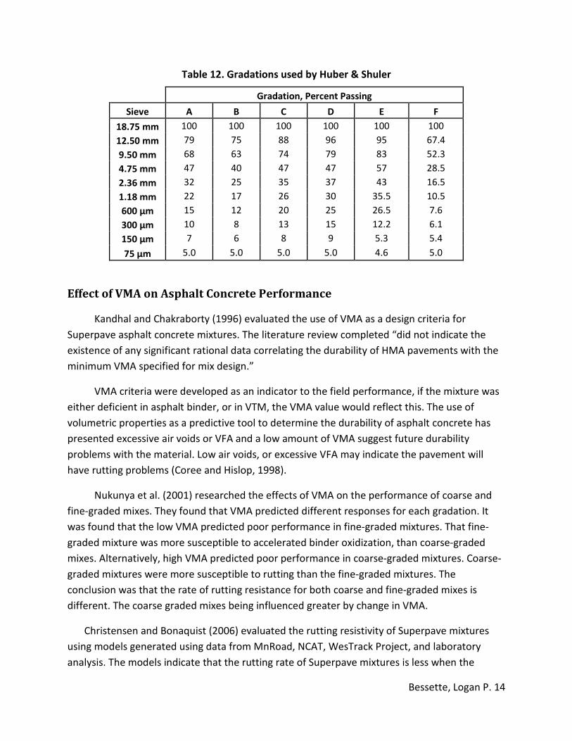
Huber and Shuler (1992) investigated the changes in VMA due to aggregate type, and

gradation. Huber and Shuler created identical gradations, with constant binder content for all

gradations and varied the aggregate between crushed limestone, and uncrushed gravel. The

testing demonstrated that the crushed limestone created a higher VMA than the uncrushed

gravel. Huber and Shuler also found that by moving gradations farther away from the maximum

density line VMA initially decreases, and then began to increase for both aggregate types, this is

presented in Table 11. Table 12 presents the gradations used.

Table 11. VMA related to distance from MDL

VMA, Percent %

Increasing Distance

from Maximum

Density Line

Crushed

Aggregate Uncrushed

Aggregate

E 13.9 12.8

D 12.6 11.0

C 11.6 10.4

A 11.5 10.8

B 12.1 10.4

F 14.4 12.4


Table 12. Gradations used by Huber & Shuler

Gradation, Percent Passing

Sieve A B C D E F

18.75 mm 100 100 100 100 100 100

12.50 mm 79 75 88 96 95 67.4

9.50 mm 68 63 74 79 83 52.3

4.75 mm 47 40 47 47 57 28.5

2.36 mm 32 25 35 37 43 16.5

1.18 mm 22 17 26 30 35.5 10.5

600 μm 15 12 20 25 26.5 7.6

300 μm 10 8 13 15 12.2 6.1

150 μm 7 6 8 9 5.3 5.4

75 μm 5.0 5.0 5.0 5.0 4.6 5.0

Effect of VMA on Asphalt Concrete Performance

Kandhal and Chakraborty (1996) evaluated the use of VMA as a design criteria for

Superpave asphalt concrete mixtures. The literature review completed “did not indicate the

existence of any significant rational data correlating the durability of HMA pavements with the

minimum VMA specified for mix design.”

VMA criteria were developed as an indicator to the field performance, if the mixture was

either deficient in asphalt binder, or in VTM, the VMA value would reflect this. The use of

volumetric properties as a predictive tool to determine the durability of asphalt concrete has

presented excessive air voids or VFA and a low amount of VMA suggest future durability

problems with the material. Low air voids, or excessive VFA may indicate the pavement will

have rutting problems (Coree and Hislop, 1998).

Nukunya et al. (2001) researched the effects of VMA on the performance of coarse and

fine-graded mixes. They found that VMA predicted different responses for each gradation. It

was found that the low VMA predicted poor performance in fine-graded mixtures. That fine-

graded mixture was more susceptible to accelerated binder oxidization, than coarse-graded

mixes. Alternatively, high VMA predicted poor performance in coarse-graded mixtures. Coarse-

graded mixtures were more susceptible to rutting than the fine-graded mixtures. The

conclusion was that the rate of rutting resistance for both coarse and fine-graded mixes is

different. The coarse graded mixes being influenced greater by change in VMA.

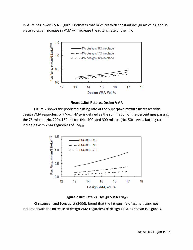
Christensen and Bonaquist (2006) evaluated the rutting resistivity of Superpave mixtures

using models generated using data from MnRoad, NCAT, WesTrack Project, and laboratory

analysis. The models indicate that the rutting rate of Superpave mixtures is less when the


mixture has lower VMA. Figure 1 indicates that mixtures with constant design air voids, and in-

place voids, an increase in VMA will increase the rutting rate of the mix.

Figure 1.Rut Rate vs. Design VMA

Figure 2 shows the predicted rutting rate of the Superpave mixture increases with

design VMA regardless of FM300. FM300 is defined as the summation of the percentages passing

the 75-micron (No. 200), 150-micron (No. 100) and 300-micron (No. 50) sieves. Rutting rate

increases with VMA regardless of FM300.

Figure 2.Rut Rate vs. Design VMA FM300

Christensen and Bonaquist (2006), found that the fatigue life of asphalt concrete

increased with the increase of design VMA regardless of design VTM, as shown in Figure 3.


Figure 3. Fatigue life vs. Design VMA

Compaction Effort

Compaction effort is the term used to describe the number of gyrations, vertical force,

and the tilt angle in the SGC (Zaniewski and Adamah, 2009). With the reduction of compaction

effort, per Table 2 and Table 3, Zaniewski and Adamah (2009) found the asphalt content

required to achieve 4.0% VTM increased by 0.5% and 0.4% for 19mm, and 37.5mm base mix,

respectively, for a design traffic of 3.0 x 106 to 30 x 10

6 ESALS.

Locking Point

The locking point concept is a technique used to determine the compaction of specimen

in the SGC. The locking point is used to determine when the aggregate particles have achieved a

dense configuration and further compaction will weaken the integrity of the aggregates. The

locking point maximizes the strength of the aggregate structure within the mix, while also

ensuring adequate space for asphalt binder to resist rutting and premature aging (Brown,

2005).

The definition of locking point has evolved over time. All methods are based on examining

the change in height versus gyration level. The current definition was defined by Vavrik (2000),

as the first of three gyrations at at the same height that are preceded by two sets of two

gyrations that are measured at the same height (Vavrik, 2000). Table 13 demonstrates an

example of the 2-2-3 locking point concept, as see in the table; the 74th

gyration indicates that

the mixture has achieved a dense configuration.


Table 13. Example of Locking Point from SGC height output

0 1 2 4 5 6 7 8 9

50 119.2 119.1* 119.0 118.9 118.8 118.7 118.6 118.5 118.5

60 118.4 118.3 118.2 118.1 118.0 117.9 117.8 117.7 117.6

70 117.6 117.5 117.5 117.4LP

117.4 117.4 117.3 117.3 117.2

*Number of gyrations: 50+1=51

Compaction Slope (k)

The compaction slope, k, was determined by using the following equations.

� = %�� − %��log�� − log��"#" ∗ 100 4

%�� = � 5

%�� = � �%��%"#" � 6

Where:

%GmmNDes is the percent of the maximum theoretical specific gravity at the design

gyrations;

%GmmNini is the percent of the maximum theoretical specific gravity after initial gyrations;

Ndes: Design number of gyrations for the compacted sample;

Nini; Initial number of gyrations for the compacted sample;

HDes: Height of compacted sample after design number of gyrations; and

Hini: Height of compacted sample after initial number of gyrations.

Vavrik (2000) found mixtures with higher compaction slopes are typically associated with

poor mixtures. The increased compaction slope indicates a high densification of mixture in the

field; high strength mixtures generally do not have high compaction slopes.

Levia and West (2008) compared the effects of asphalt content, and aggregate ratios on

the interlocking of aggregate particles in asphalt concrete and the impact on the compatibility

of mixtures in the field. They found mixtures with higher asphalt contents have higher

compaction slopes for the same gradation. Fine gradations and mixtures with rounded

aggregates have lower compaction slopes. The mixtures with higher compaction slopes

generally have lower permanent shear strains and increased shear stiffness.


Indirect Tensile Strength

The indirect tensile (IDT) strength test is a test to determine the performance

characteristics of asphalt concrete mixtures. The equipment is available to most agencies. The

IDT strength test is performed by loading a cylindrical asphalt specimen with a vertical force, as

should in Figure 4.

Figure 4. IDT strength test, prior to failure, and failed specimen

The curved loading strips on the top, and bottom of the specimen apply a compression

force. The interaction of the stresses causes a tension failure along the vertical diametral plane

as shown on Figure 4(b). The peak load that specimen can withstand is recorded and used in

the following equation to determine the IDT strength of the specimen.

&' = 2�)*+

7

Where: σx: Horizontal tensile strength at the center of the specimen;

P: Peak applied load;

d: diameter of the specimen (inches); and

t: Thickness of the specimen (inches).

The IDT strength is used as an indicator for the mixtures performance with respect to

rutting, thermal cracking, and fatigue cracking (Christenson and Bonaquist, 2000). The test is

considered a quick test, with low loads, that can adequately present the properties of the

mixture (Christenson and Bonaquist, 2002). The second generation of high temperature IDT

strength testing provides recommended requirements for IDT strength as a fuction of traffic

level (Christenson and Bonaquist, 2007). IDT strength was presented as a good indicator of the


rut depth of asphalt concrete testing compared to the Asphalt Pavement Analyzer (APA)

(Zaniewski and Srinivasan, 2003). As shown in Figure 5.

Figure 5. Rut Depth vs. IDT Strength

Wen and Bsuhal (2013) found that using asphalt mixture performance tester (AMPT),

with the IDT jig attachment could help predict fatigue life. Using the fracture energy, the area

under the stress-strain plot of a loaded specimen up to the peak stress, they could predict the

fatigue life of the asphalt concrete with good confidence. The fracture energy is found

mathematically by taking the integral of the function that presents the curvature of the line.

AMPT uses digital instrumentation to capture this data. Figure 6 presents the results of the

fracture energy versus the predicted fatigue life using AMPT.

Figure 6. IDT Fracture Energy vs. Fatigue Life (Cycles)


Film Thickness

Film thickness is used to describe the thickness of the asphalt film surrounding aggregate

particles in an asphalt concrete mixture; it is often referred to as either the apparent film

thickness (AFT), or the average film thickness.

Kandhal et al. (1998) published their findings on factors that affect the durability of

asphalt mixtures. The report emphasizes the need to optimize the film of asphalt binder that

coats the aggregate particles rather than use a broad requirement such as a minimum VMA for

a given NMAS. Their analysis determined that high permeability, high air voids, and thin asphalt

coats on the aggregate all lead to excessive binder aging and decrease the durability of the

mixture in the field. They recommended that an asphalt coating of 8 microns be used to ensure

pavement durability.

Testing completed by Christensen and Bonaquist (2006) was analyzed to understand the

correlation between the performance of asphalt pavements and the AFT. The basic equation is

(Christenson and Bonaquist, 2006):

� � = �,�-.� ∗ / �1,000 8

Where:

AFT: Average Film Thickness, microns;

Vasp: Effective volume of asphalt, liters;

SA: Computed surface area of aggregate, m2/kg; and

W: Mass of aggregate, kg

Aggregate Surface Area

An alternative to the use of VMA criteria is the use of asphalt film thickness coating

aggregate to determine a durable mix design. This concept was introduced in by Richardson

(1905) with his determination that the amount of asphalt:

“in any mixture should be sufficient to thickly coat every particle of mineral matter and

fill the voids in the sand… without making the resulting asphalt surfaces too susceptible

to temperature changes.”

Richardson found asphalt mixtures needed a minimum asphalt content that would allow

the samples to be stable, and resistant to fatigue cracking. Asphalt concrete that was deficient

in binder would become brittle, and become highly susceptible to thermal cracking.


Richardson found that the proper asphalt content was different for various mineral

aggregates, many ranging from 9% to 14%. Fine mixtures require a larger amount of asphalt

than a coarse mixture using the same source mineral aggregate. Richardson expressed that as

the diameter of an aggregate particle became smaller, the surface area in square centimeters

per gram of mass increase rapidly (Richardson 1905). Table 14 presents Richardson’s findings.

Table 14. Surface area for one gram of uniform sand

One Gram of Uniform Sand

Mesh Sieve Opening

(mm)

Number of

Particles

Surface Area

(cm2)

10 1.5 213 15

20 0.84 1,216 27

30 0.58 3,694 39.4

40 0.4 11,261 56.6

50 0.26 41,005 87.1

80 0.2 90,066 113.2

100 0.13 328,032 174.2

200 0.075 1,407,320 283

In 1918, Edwards, an engineer working to improve methods of designing Portland

cement concrete mixes, evaluated the use of surface area to design mixes (Hveem 1936).

Edwards worked to estimate the both the volume, and mass of each aggregate particle and

assign a surface area factor to estimate the specific surface area of aggregates. Hveem

published Edward’s work regarding the determination of the surface area constant for particles

that passed the #200 sieve (Hveem 1936).

Surface area is a function of the gradation of the blended stockpiles, creating unique

surface area factors for each gradation. The gradation is found using AASHTO T27 Sieve Analysis

of Fine and Coarse Aggregates; the mass retained on each sieve is used to determine the

percentage of the aggregate passing each sieve.

Surface area is computed using Equation 9 (Roberts et al., 2009):


.� = 1�. " ∗ �" 9

Where:

SA: Surface Area of gradation;

SFi: Surface Factor for sieve i; and

Pi: Cumulative percent passing sieve i, in decimal notation.

Surface area calculations are based on the assumption that the diameter of the

aggregate particles is equivalent to the size or the opening of the sieve that a particle passed

though, Edward’s assumed that the particles were spheres with smooth sides. Table 15

contains the surface area factors used by Hveem, adopted from Edwards work, Hveem’s initial

estimates in 1936, and those by Zaniewski and Reyes Daverage method (Zaniewski and Reyes,

2003).

Table 15. Surface Area Factors, based on Percent Passing

Sieve Size >4.75 mm 4.75 mm 2.36 mm 1.16 mm 600μm 300μm 150μm 75μm

Surface

Area Factor

(ft2/lb)

2 2 4 8 14 30 60 160

Surface

Area Factor

(m2/kg)

0.41 0.41 0.82 1.64 2.87 6.14 12.29 32.77

Hveem

1936

(ft2/lb)

2 4 8 16 30 60 120 200

Hveem

1936

(m2/kg)

0.41 0.82 1.64 3.28 6.14 12.29 24.58 40.96

Zaniewski

and Reyes

Davg (ft2/lb)

1.6 3.1 6.3 12.4 24.6 49.1 98.3 294.8

Zaniewski

and Reyes

Davg

(m2/kg)

1

0.32 0.64 1.28 2.54 5.03 10.06 20.13 60.38

Note1: Zaniewski and Reyes Davg method uses percent retained on the sieve


The surface area of the material minus No. 200 sieve is important because of the large

specific area of the mineral particles. Zaniewski and Reyes (2003) used the Blaine Air

Permeability Apparatus, Figure 7, to measure the surface area of the material passing the No.

200 sieve (75 µm). The measured surface area for materials smaller than 75 microns are larger

than the value , 32.77 m2/kg estimated by Hveem, Zaniewski and Reyes’ results are presented

in Table 16.

Figure 7. Air Permeability Apparatus

Zaniewski and Reyes (2003) also recommended the use of percent retained on

individual sieves to calculate the surface area rather than using the cumulative percent passing

by Hveem. It is presented as a more defendable and logical practice because percent passing

method can be flawed because the percent passing each sieve is a function of the mass

retained on all prior sieves.

Table 16. Specific area for material less than 75 microns

Aggregate Source

Average Tested

Surface Area

(m2/kg)

Summersville 458

Beaver Boxley (A) 435

Beaver Boxley (B) 289

APAC Sand 478

APAC #10 437

New Enterprise 615

Natural Sand 118


Christensen and Bonaquist (2006) correlated data between the summation of the

percent passing the 75-, 150-, and 300 μm sieves (FM300) and the aggregate specific surface

area calculation. Also correlation between the percent passing the 75 microns sieve (P75) and

the aggregate specific surface area (Christensen and Bonaquist, 2006) was completed. The

method for calculating the aggregate specific surface area was not outline, however it is

assumed to be constant for all mixes. The research showed that the FM300 is a better indication

of surface area than the percent material passing the 75µm sieve. This report demonstrates

that a confident prediction of surface area comes from the materials smaller than 300 microns.

Figure 8. Surface Area vs FM300

Figure 9. Surface Area vs. P75


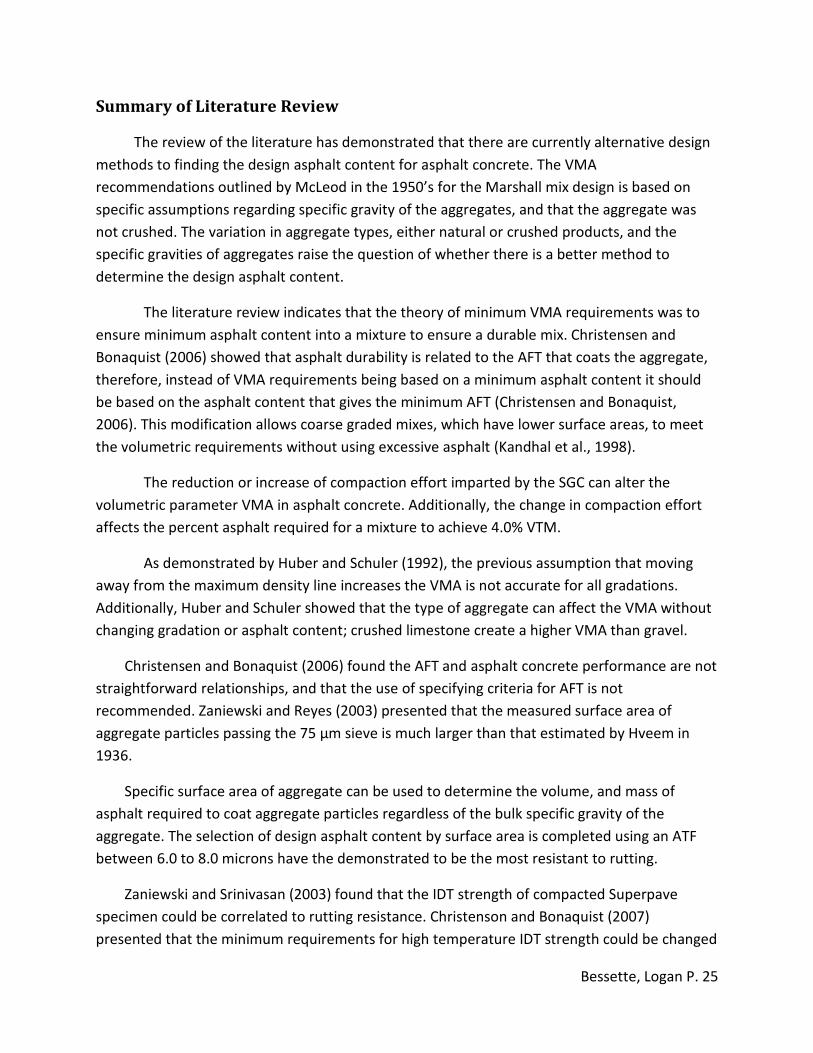
Summary of Literature Review

The review of the literature has demonstrated that there are currently alternative design

methods to finding the design asphalt content for asphalt concrete. The VMA

recommendations outlined by McLeod in the 1950’s for the Marshall mix design is based on

specific assumptions regarding specific gravity of the aggregates, and that the aggregate was

not crushed. The variation in aggregate types, either natural or crushed products, and the

specific gravities of aggregates raise the question of whether there is a better method to

determine the design asphalt content.

The literature review indicates that the theory of minimum VMA requirements was to

ensure minimum asphalt content into a mixture to ensure a durable mix. Christensen and

Bonaquist (2006) showed that asphalt durability is related to the AFT that coats the aggregate,

therefore, instead of VMA requirements being based on a minimum asphalt content it should

be based on the asphalt content that gives the minimum AFT (Christensen and Bonaquist,

2006). This modification allows coarse graded mixes, which have lower surface areas, to meet

the volumetric requirements without using excessive asphalt (Kandhal et al., 1998).

The reduction or increase of compaction effort imparted by the SGC can alter the

volumetric parameter VMA in asphalt concrete. Additionally, the change in compaction effort

affects the percent asphalt required for a mixture to achieve 4.0% VTM.

As demonstrated by Huber and Schuler (1992), the previous assumption that moving

away from the maximum density line increases the VMA is not accurate for all gradations.

Additionally, Huber and Schuler showed that the type of aggregate can affect the VMA without

changing gradation or asphalt content; crushed limestone create a higher VMA than gravel.

Christensen and Bonaquist (2006) found the AFT and asphalt concrete performance are not

straightforward relationships, and that the use of specifying criteria for AFT is not

recommended. Zaniewski and Reyes (2003) presented that the measured surface area of

aggregate particles passing the 75 μm sieve is much larger than that estimated by Hveem in

1936.

Specific surface area of aggregate can be used to determine the volume, and mass of

asphalt required to coat aggregate particles regardless of the bulk specific gravity of the

aggregate. The selection of design asphalt content by surface area is completed using an ATF

between 6.0 to 8.0 microns have the demonstrated to be the most resistant to rutting.

Zaniewski and Srinivasan (2003) found that the IDT strength of compacted Superpave

specimen could be correlated to rutting resistance. Christenson and Bonaquist (2007)

presented that the minimum requirements for high temperature IDT strength could be changed


as a function of the travel level. Mixes with higher IDT strength have greater resistance to

rutting. Wen and Bsuhal (2013) found fatigue life could be predicted from the fracture energy

of the compacted mixture. Mixes that had large areas under the stress-strain diagram when

completing the IDT strength test, could withstand greater fatigue cycles in the AMPT.


CHAPTER 3 RESEARCH METHODOLOGY

Introduction

This research evaluated the effects of changing the aggregate gradation, and compaction

effort on VMA. The current specifications that are recommended by both the Asphalt Institute

and the American Association of State and Highway Transportation Officials, are based on

volumetric analysis of asphalt pavements, the components VFA, VTM, and VMA are given

design ranges to control the durability and performance of the pavements used in West

Virginia, and the United States. However, because VMA is often the most difficult parameter to

satisfy it was the focus of this research.

The Superpave 9.5mm mix design was supplied from J.F. Allen Company in Elkins, WV. All

aggregate were crushed limestone. The contractors design binder content was 6.2% at 80

gyrations. The research approach involved:

• Obtain aggregate and binder from J.F. Allen Company

• Sieving aggregate on all U.S. customary sieves, 12.5mm, 9.5mm, No. 4, No. 8, No. 16,

No. 30, No. 50, No. 100, and No. 200.

• Wash aggregate to remove fines, and oven dry to constant mass, place in bins for

storage, bag house fines were used to supplement the amount of No. 200 material

needed in the mixes.

• Blend aggregates to create the three gradations.

• Create specimens for compaction in SGC, and maximum theoretical specific gravity.

• Complete volumetric analysis in accordance with WVDOH specifications.

• Test samples for IDT strength, and compute the force –deformation fracture energy as

captured from the IDT strength curve.

• Complete statistical analysis of data collected.

Experiment Design

The experiment was evaluated with three factors; compaction effort, aggregate

gradation, and asphalt content. The compaction efforts were 80 gyrations and 100 gyrations.

The aggregate gradations were coarse, design, and fine-graded.

For the experimental design it was desirable to use consistent levels of percent binder for

all combinations of compaction level and gradation. The contractor’s design binder content was

6.2% for 80 gyrations. Based on previous experience, it was anticipated that this was 0.4%

greater than would be needed for the same gradation at 100 gyrations. The binder adjustment

for gradation would suggest the binder would be greater for the fine blend and lower for the


coarse gradation. Considering these factors, it was decided to “center” the percent binder in

the experiment at 6.0% The other binder levels were set at +/- 0.5% and +/- 1.0%., i.e. the

percent binder levels used in the experiment were 5.0%, 5.5%, 6.0%, 6.5% and 7.0%. Table 17

presents the testing matrix used for this research. Three replicate samples were produced for

each combination of factors and levels. Analysis of Variance (ANOVA) was used to evaluate the

significance of the factors. When the samples were determined to be statistically different, the

Tukey-Kramer Honest Significant Difference test was used to determine which variable were

different. A total of 90 compacted specimens, and 45 maximum theoretical specific gravity

samples were prepared and tested.

Table 17. Testing matrix

NMAS 9.5 mm

Compaction Effort 80 Gyration 100 Gyrations

Gradation Coarse Contactor Fine Coarse Contactor Fine

Asphalt Content

5.0% 1 2 3 16 17 18

5.5% 4 5 6 19 20 21

6.0 % 7 8 9 22 23 24

6.5% 10 11 12 25 26 27

7.0% 13 14 15 28 29 30

Gradations

The aggregate blend received from J.F. Allen Company was used as the starting point for

creating aggregate gradations. The fine and coarse gradations were created by satisfying the

following criteria,

• Gradation could be achieved by blending contractor stockpiles

• Gradation was within control points of WVDOH 9.5mm NMAS specifications

• Gradations created maximum separation of coarse and fine mixes

• Remain approximately 5% away from control points for practicality.

Figure 10 present the gradation curves for the 9.5 mm mixes that were created,

summary table for the aggregate blending are in the appendix.


Figure 10. 9.5mm Aggregate Gradations

12

.5

9.5

4.7

5

2.3

6

1.1

8

60

0µ

m

30

0µ

m

15

0µ

m

75

µm

0%

10%

20%

30%

40%

50%

60%

70%

80%

90%

100%P

erc

en

t P

ass

ing

(%

)

Sieve (mm)

Coarse

Fine

Contractor

Control

PointsMDL


Sample Creation

Weigh out tables were created for each gradation to determine the mass of aggregate

from each stockpile to use in the mix. The aggregate, binder, and mixing tools were heated to

the mixing temperature of 157°C. Once at the design mixing temperature the aggregate was

added to the mixing bucket. A small crater was created in the center of the hot aggregate and

the correct mass of binder was poured into the creator. The aggregate and binder were then

mixed together in the bucket mixer until all aggregate particles were covered with binder. The

amount of material in each batch was sufficient to make 2 compacted, and one maximum

specific gravity samples.

Upon completion of mixing, the mix was placed in the oven to condition at the

compaction temperature of 145°C for two hours with stirring after one hour. Once the mix had

conditioned for two hours, it was poured into a SGC mold that was heated to the compaction

temperature. The mold with the mixture was placed in the SGC and compacted to either 80, or

100 gyrations. After compaction the specimen was allowed to cool to room temperature before

completion of the volumetric analysis. The specimens created for the maximum theoretical

specific gravity samples were created in the same procedure as the compacted specimen, but

after the two hour conditioning time it was spread out on a non-absorbing surface to cool to

room temperature.

Analysis

The volumetric analysis used AASHTO T166, Bulk Specific Gravity of Compacted Hot Mix

Asphalt (HMA) using Saturated Surface Dry Specimens, T209, and Theoretical Maximum Specific

Gravity and Density of Hot Mix Asphalt (HMA), T269, Percent Air Voids in Compacted Dense and

Open Asphalt Mixtures, using the following equations:

�� = � − � � ∗ 100 10

�� = �100 − �� 11

� � = �� − �� ∗ 100 12

Where,

Gmm= Maximum theoretical gravity of mixture;

Gsb= Bulk specific gravity of aggregate;


Ps= Percent stone, and,

Gmb= Bulk specific gravity

IDT Strength Testing

The IDT strength of the asphalt specimen were found by testing the SGC pills. The pills

ranged from 110 mm to 120 mm in height and had diameter of 150 mm. Prior to testing the

pills, they were submerged in a 60°C water bath for 1 hour and 15 minutes. The temperature of

60°C was used because it is the standard temperature for Marshall stability testing, and the

time of saturation was increased to account for the increased volume of the Superpave

specimem. The Marshall stability apparatus that was used for testing applied a constant

deformation rate of 50mm/min. The strength of each sample was computed using Equation 7.

Fracture Energy

The fracture energy for each specimen was calculated by importing the load vs.

deformation curve from the IDT test into AutoCad and completing a set of data manipulations.

The order of operations was as follows:

• Import laboratory curve into AutoCad and ensure proper scale.

• Find point of peak load and draw line perpendicular to the abscissa.

• Use “Spline” command to outline the lab curve from point (0,0) to peak load.

• Use “area” command by “polyline” to calculate the area under the load

deformation curve.

Locking Point and Compaction Slope

The locking point, and compaction slope of each mixture was determined for each

mixture. The 2-2-3 locking point was used all mixes, the compaction slope was calculated using

Equations 2, 3, and 4.

Statistical Analysis

After the laboratory tests where completed, a variety of statistical analysis methods

were used to determine the significance of the results. The Analysis of Variance (ANOVA), linear

regression, and the Tukey Kramer Honest Significant Difference test (HSD) were used. The

background regarding the statistical methods follows.

ANOVA

The one way ANOVA analysis was used to determine if there was a significant difference

between groups of data. This is a statistical method for comparing several sample means, and


assumes the null hypothesis (Ho) that all means are equal, and the alternative hypothesis(Ha)

that not all means are equal (Moore et al., 2012).

Ho : µ1 = µ2 = … = µi

13

Ha: not all µi are equal 14

Where:

µ1: mean of sample 1;

µ2: mean of sample 2; and

µi: mean of the ith

sample.

An assumption for the ANOVA analysis is the group varied by a single factor, an example

of this was: “At 80 gyrations, and 5% binder, how do the IDT strengths of coarse, fine, and

contractor graded mixes compare?” The null hypothesis will be rejected if the F-statistic, a

function of the degrees of freedom in the numerator and denominator, is larger than F-critical

at the 95% confidence interval. If the F-statistic is less than F-critical, the null hypothesis is

accepted.

Tukey Kramer Honest Significant Difference (HSD)

The Tukey Kramer HSD is a method of multiple comparison used in conjunction with

ANOVA to determine if two means are equal when the F-test rejects the null hypothesis

(Dowdy et al., 2004). The test compares means over a confidence interval by means of 15

23" − 342 ≥ 6∝,,,,�#89 :�.;<

15

Where:

Yi= average of group i;

Yj= average of group j;

qα,a,a(n-1)= q-statistic as a function of degrees of freedom in numerator,

denominator and confidence interval.

MSe= mean square of error,

n= number of samples.

Linear Regression

A linear regression line is a straight line that predicts how dependent variable y changes

as independent x changes. This is accomplished by fitting a line with slope b1 and intercept bo to

the data. The equation for the line is presented as:

3 = => + =9@ 16


Using Equation 16, a response value for y can be plotted for any value of x. The quality

of prediction is indicated by R2, the fraction of variation. An R

2 =1.00 indicates that the

regression line exactly predicts the value of y for any change in x.

AB = ∑�3D" − 3E" B∑�3" − 3E" B 17

Where:

∑�3D" − 3E" B= variance of predicted values3D; and

∑�3" − 3E" B= variance of observed values y.

Summary of Research Methodology

To properly evaluate the effect of aggregate gradation, compaction effort, and asphalt

content on VMA the following steps were required.

• Blend of stockpiles to create three gradations that exhibit high surface area, moderate

surface area, and low surface area.

• Create specimens with 5.0%, 5.5%, 6.0%, 6.5% and 7.0% asphalt content.

• Compute the volumetric properties in accordance with the West Virginia Department of

Highways Material Procedures.

• Test samples for IDT strength and compute the fracture energy.

• Development of analysis procedures for determining relationships between compaction

effort, aggregate gradation, and volumetric properties.


CHAPTER 4 RESULTS AND ANALYSIS

The samples created were evaluated for volumetric properties, locking point, compaction

slope, IDT strength, and fracture energy. The design binder content for each mix was

determined for both 80, and 100 gyrations. Once the volumetric properties were determined,

the specimens were tested for IDT strength after curing for 24-hours. The relationships

between volumetric properties, compaction effort, asphalt film thickness, fracture energy and

IDT strength were evaluated.

Mix Properties

The first analysis performed on the data was to evaluate the data to determine the design

binder content and associated properties as summarized in Tables 19 and 20. The volumetric

plots in the appendix were used to determine Pb at 4.0% VTM for each mix. Then the other

volumetric properties were selected at their respective value of Pb dependent on the

combination of gradation and compaction. The results obtained from the research data area

compared to the WVDOH criteria for 9.5mm mixes.

The volumetric parameters and other performance indicators at the design binder contents

are presented in Table 18. Figures showing the properties are presented in the appendices.

For both compaction levels the design binder content for the contractor gradation is less

than the design binder content for the fine and coarse gradations. This is a reasonable result as

the gradation curves for the fine and coarse gradations are further away from the maximum

density line than the contractor design blend, especially for the aggregates passing the No. 16

sieve.

Table 18. Volumetric Properties at 4.0% VTM, 80 Gyrations

80 Gyrations

Coarse Fine Contractor Criteria

Pb 7.0% 6.8% 6.4% -

VTM 4.0% 4.0% 4.0% 4.0%

VMA 18.2% 17.2% 16.8% 15.5%

VFA 78% 78% 75% 74% - 80%

Pbe 6.3% 5.7% 5.6% -

d/Pbe 0.76 1.15 0.96 0.6 – 1.2


Table 19. Volumetric Parameters at 4% VTM, 100 Gyrations

100 Gyrations

Coarse Fine Contractor Criteria

Pb 6.8% 6.6% 6.1% -

VTM 4.0% 4.0% 4.0% 4.0%

VMA 18.0% 16.7% 16.1% 15.5%

VFA 78% 76% 75% 74% - 80%

Pbe 6.1% 5.5% 5.3% -

d/Pbe 0.79 1.2 1.02 0.6 – 1.2

Table 20 provides additional mix properties that were interpolated from the data

collected from the asphalt contents around the respective design binder content, as indicated

in Table 18 and Table 19. The coarse, and fine mixtures have less IDT strength than the

contractors gradation. As the gradation moves from coarse to fine the compaction slope

decreases. As anticipated the coarse gradation had the highest ATF.

Table 20. Mix Properties at Design Binder Content*

Gradation

Coarse Fine Contractor

80

Gyrations

Tf (microns) 14.2 9.08 11.0

Compaction

Slope (k) 10.6 9.6 10.0

IDT (psi) 15.1 16.2 17.5

100

Gyrations

Tf (microns) 13.7 8.8 10.3

Compaction

Slope (k) 9.9 9.3 9.4

IDT (psi) 12.2 15.5 15.7

*Average for 3 Samples

• The 80 gyration mixes required more design binder than the 100 gyration mixes.

• The coarse, and fine gradations had higher VMA than the contractor gradation due

to the increased distance from the maximum density line.


• The contractor gradation had the largest change in VMA when changing from 80-

to 100 gyrations.

• The coarse graded, 80 and 100 gyration mix had a VMA that was greater than the

WVDOH recommendation stating that mixes with VMA more than 2% higher than

the specification are susceptible to rutting and have tendency to shove under the

roller.

The 100 gyration mixture produced lower VMA than the 80 gyration. As anticipated the

coarse and fine gradations, which are far away from the maximum density line, achieve the

highest the VMA. The contractor gradation has the largest change in VMA when changing the

compaction level from 100 to 80 gyrations.

According to the literature, the percent binder required to achieve 4% VTM at Ndesign is

less when using higher compaction effort. The fine and coarse gradations both required 0.2%

less binder when changing the compaction level from 80 to 100 gyrations; the contractor

gradation required 0.3% less binder.

The VMA change was less than seen by Huber and Anderson (2004).When reducing the

gyration by 20, the change in VMA was 0.2%, 0.5%, and 0.7% for the coarse, fine, and

contractor gradations, respectively. This is less than the 1.0% change reported by Huber and

Anderson (2004) when decreasing Ndesign by 25 gyrations.

Surface Area and Film Thickness

The specific surface area of the gradations were found using two methods; the Hveem

method using cumulative percent passing, Zaniewski and Reyes (2004) Davg method with

individual percent retained. The surface area calculation using the P200 constants determined by

Zaniewski and Reyes (2004) was not used for this research. Table 21 shows the Hveem method

resulted in higher surface areas than the Daverage method for each gradation. For consistency

with the literature the Hveem method was used for all following analysis.

Table 21. Calculated Surface Areas

Method

Hveem Davg

Gradation (m2/kg)

Coarse 4.65 4.42

Fine 6.66 6.29

Contractor 5.33 5.05


Figure 11 demonstrates the differences in calculated surface area between the methods.

Figure 11. Calculated Surface Area, Davg vs. Hveem

Film Thickness

The film thickness was calculated using Equation 6. The mixtures had film thickness

between 6.4 microns (Fine gradation, 5.0% binder) and 14.9 microns (Coarse Gradation, 7.0%

binder) when using the Hveem method of surface area calculation. There was not an optimum

asphalt film thickness to be applied to all gradation. Kandhal et al. (1998) recommended film

thickness should be in the range of 9 to 10 microns

Indirect Tensile Strength

Zaniewski and Srinivasan (2003) correlated IDT strength and APA results to allow the use

of IDT as an indicator of rutting potential, shown in Figure 5. Using an APA limit of 8 mm (Brown

et al., 2001) an IDT strength greater than 12 psi indicates a suitable mix with respect to rutting.

Figure 12 and 13 shows that the IDT strength of the specimen increase with film

thickness for each gradation at both compaction levels. The coarse gradation presented the

lowest IDT strength although it had the largest film thickness. The contractor gradation created

the highest IDT strengths.

4

4.5

5

5.5

6

6.5

7

4 4.5 5 5.5 6 6.5 7

Av

era

ge

Dia

me

ter

Su

rfa

ce A

rea

(m

2/k

g)

Hveem Surface Area (m2/kg)

Line of

equality


Figure 12. Relationship between IDT strength and film thickness at 80 gyrations

Figure 13. Relationship between IDT strength and film thickness at 100 gyrations

11.0

12.0

13.0

14.0

15.0

16.0

17.0

18.0

19.0

6.0 8.0 10.0 12.0 14.0 16.0

ID S

tre

ng

th (

psi

)

Film Thickness (microns)

Coarse

Fine

Contractor

8.0

10.0

12.0

14.0

16.0

18.0

20.0

4.0 6.0 8.0 10.0 12.0 14.0 16.0

ID S

tre

ng

th (

psi

)


Coarse

Fine

Contractor


Fracture Energy

Fracture energy, as calculated by Wen and Bsuhal (2013) was accomplished by finding

the area under the stress-strain diagram of an asphalt specimen loaded using the AMPT with

IDT jig. They found that fracture energy can be used to calculate the number of fatigue cycles a

specimen could endure with good confidence, Figure 6.

To simulate the Wen and Bsuhal method, the area under the load-deformation diagram

from the IDT test was calculated for all specimens. Each graph was digitized, and then imported

into AutoDesk® AutoCad, as presented in Figure 14. A spline polyline was fit to the curve of

each specimen, and then the area function was used to find the fracture energy (lb-inch).

Figure 14. Example Fracture Energy from IDT Load Diagram

The calculated fracture energy was used to compare the estimated fatigue life of the 80

and 100 gyration samples. The fracture energy for the 80 gyration samples were on average

32% greater than the 100 gyration samples. Table 22 presents the fracture energy (lb-in), IDT

strength (psi), and percent difference for all samples.


The IDT strength and fracture energy data are shown on Figure 15. The coefficient of

determination, R2 of the trendline is 0.61. The coarse, 80 gyration samples have fracture energy

that is similar to the contractors 80 gyration mixes, although having lower IDT strength.

According to Wen and Bsuhal (2013), this indicates the two mixes will have similar fatigue life,

while the larger AFT of the coarse mixture will resist oxidization better than the fine, and

contractor mix.


Figure 15. Fracture Energy vs. IDT Strength

y = 2.9735x - 2.5449

R² = 0.6067

0

10

20

30

40

50

60

10 11 12 13 14 15 16 17 18 19

Fra

ctu

re E

ne

rgy

(lb

-in

)

IDT Strength (psi)

Coarse 80

Fine 80

Contractor 80

Coarse 100

Fine 100

Contractor 100


Table 22. IDT Strength and Fracture Energy

IDT Strength (psi) Fracture Energy (lb-in)

Percent

Binder

80

Gyration

100

Gyration

Percent

Difference 80

Gyration

100

Gyration

Percent

Difference

Coarse 5.0% 11.9 10.1 17.8% 40.8 30.3 34.5%

5.5% 14.5 11.8 22.9% 47.4 33.1 43.1%

6.0% 14.6 11.3 29.2% 47.6 28.9 65.1%

6.5% 15.3 11.8 29.6% 48.2 32.4 48.9%

7.0% 15.1 12.5 20.8% 54.1 33.8 60.4%

Fine 5.0% 13.4 14.1 -5.0% 35.9 33.5 7.0%

5.5% 15.2 14.2 7.0% 42.2 37.7 12.1%

6.0% 15.9 13.5 17.8% 43.1 25.9 66.7%

6.5% 16.0 15.4 3.9% 44.4 35.8 24.1%

7.0% 16.3 15.9 2.5% 46.9 41.6 12.6%

Contractor 5.0% 15.6 14.9 4.7% 42.5 35.9 18.6%

5.5% 17.3 13.9 24.5% 46.9 33.4 40.3%

6.0% 17.8 15.8 12.7% 51.2 43.6 17.6%

6.5% 17.2 15.7 9.6% 50.0 40.9 22.1%

7.0% 17.5 18.3 -4.4% 52.1 52.5 -0.7%

Locking Point

The 2-2-3 locking point was not achieved for any mix at 80 gyrations. The average number

of gyration to achieve locking point was determined from the 3 compacted specimens at each

unique gradation and binder content. Table 23 presents these data. Cells that do not contain


data had at least one specimen that did not achieve locking point, all fine graded mixes had a

minimum of one specimen failing to lock out within 100 gyrations. The failure to achieve lock

out by the fine mix indicates that the aggregate structure of the asphalt concrete is not in a

dense configuration.

Table 23. Gyrations to achieve locking point

Gradation

Percent Binder Coarse Fine Design

5.0% 85 - 94

5.5% 90 - 95

6.0% - - 92

6.5% 93 - -

7.0% 91 - -

The fine gradation mixture did not lock out in accordance with the 2-2-3, this mixture

also had the lowest asphalt film thickness, and lowest compaction slope. The locking point data

are in the appendices.

Figure 16 shows compaction slope (k) is influenced by film thickness, the thicker asphalt

coating the steeper the compaction slope. Vavrik (2000) found mixes with high compaction

slopes generally have poor performance because of rapid densification in field construction.

The coarse graded mixture had the highest compaction slope, and the lowest IDT strength of

the specimens tested.


Figure 16. Compaction slope vs. Film thickness

y = 0.1853x + 7.5571

R² = 0.6812

7.00

8.00

9.00

10.00

11.00

5.00 6.00 7.00 8.00 9.00 10.00 11.00 12.00 13.00 14.00 15.00

Co

mp

act

ion

Slo

pe

(k

)


Coarse 5.0%

Coarse 5.5%

Coarse 6.0%

Coarse 6.5%

Coarse 7.0%

Fine 5.0%

Fine 5.5%

Fine 6.0%

Fine 6.5%

Fine 7.0%

Contractor 5.0%

Contractor 5.5%

Contractor 6.0%

Contractor 6.5%

Contractor 7.0%


Comparison between the dust-to-effective binder ratio, and the dust-to-film thickness

ratio (percent dust to film thickness in microns) was completed as part of this research. Under

WVDOH specifications, the dust-to-effective binder ratio must be 0.6-1.2 for fine graded mixes,

or 0.8-1.6 for coarse graded mixes. The film thickness was calculated using the effective asphalt

binder and the surface area of the aggregate calculated by the Hveem method.

Figure 17. Dust-to-film thickness ratio vs. dust-to-effective binder ratio

Figure 17 shows that there is a relationship between the dust-to-film thickness ratio and

the dust-to-effective binder ratio. As seen in the figure, the dust to effective binder ratio has a

larger range than the dust to film thickness ratio.

Comparison of IDT Strength and Compaction Effort

Analysis of the effect of compaction effort on the IDT strength was completed for each

of the gradations. Figures 18, 19, and 20 show the IDT strength of the mixes compacted to 80

gyrations was higher than that of the 100 gyration mixes. This trend was consistent for each

gradation level

y = 0.8038x - 0.32

R² = 0.9295

0.00

0.50

1.00

1.50

2.00

0.00 0.50 1.00 1.50 2.00

d/T

f

d/Pbe


Figure 18. IDT Strength vs. percent binder for Coarse gradation

Figure 19. IDT Strength vs. Percent binder, Fine gradation

y = 1.4417x + 5.6459

R² = 0.6091

y = 0.975x + 5.6638

R² = 0.4915

10.0

11.0

12.0

13.0

14.0

15.0

16.0

17.0

4.5 5 5.5 6 6.5 7 7.5

ID S

tre

ng

th (

psi

)

Percent Binder (%)

Coarse Gradation

80 Gyration

100 Gyration

y = 1.2912x + 7.6177

R² = 0.6507

y = 0.9478x + 8.9465

R² = 0.3719

12.0

13.0

14.0

15.0

16.0

17.0

4.5 5 5.5 6 6.5 7 7.5

ID S

tre

ng

th (

psi

)

Percent Binder (%)

Fine Gradation

80 Gyration

100 Gyration


Figure 20. IDT Strength vs. Percent binder, Contractor gradation

ANOVA Summary

Comparison of Gyrations

The Analysis of Variance was used to determine if there was a statistical difference

between the IDT strength determined for the 80 and 100 gyration mixes with a significance

level of P= 0.05, indicating a 95% confidence interval. As indicated in the research approach, a

p-value less than 0.05 indicate that the means are not equal, and there is insufficient evidence

to reject the null hypothesis.

The Tukey-Kramer honest significant difference (HSD) analysis was used to determine if

one gradation was significantly different than the others once the ANOVA analysis had found

there was a significant difference amongst the group. The analysis tables for IDT strength at 100

gyrations are shown in Table 24 and Table 25, and Table 26 and Table 27 for 80 gyrations.

y = 0.7297x + 12.705

R² = 0.3338

y = 1.6964x + 5.5314

R² = 0.4848

12.0

13.0

14.0

15.0

16.0

17.0

18.0

19.0

4.5 5 5.5 6 6.5 7 7.5

ID S

tre

ng

th (

psi

)

Percent Binder (%)

Contractor Gradation

80 Gyration

100 Gyration


Table 24. IDT Strength for 100 Gyrations

Anova: Single

Factor

SUMMARY

Groups Count Sum Average Variance

Coarse 1 15 172.71 11.514 1.036

Fine 2 15 219.49 14.633 1.294

Contractor 3 15 235.64 15.709 3.180

ANOVA

Source of Variation SS df MS F P-value F crit

Between Groups 142.47 2 71.23 38.78 2.87E-10 3.219942

Within Groups 77.144 42 1.837

Total 219.61 44

Table 25. Tukey-Kramer Multiple Comparisons, 100 Gyrations

Coarse Gradation 1 11.51

n Group 1 15

Fine Gradation 2 14.63

n Group 2 15

Contractor Gradation 3 15.71

n Group 3 15

MSe 1.84

Q Statistic 3.44

Comparison of Group 1 to Group 2

Absolute Difference 3.1191

Standard Error of Difference 0.3499

Critical Range 1.2038

Means of Groups 1 and 2 are Different










Means of Groups 2 and 3 are Not Different


Table 26. IDT Strength for 80 Gyrations

Anova: Single

Factor

SUMMARY


Coarse 15 214.4406 14.29604 1.828064

Fine 15 230.4736 15.36491 1.372532

Design 15 256.2513 17.08342 0.8546

ANOVA


Between Groups 59.32617 2 29.66309 21.9445 2.99E-07 3.219942

Within Groups 56.77276 42 1.351732

Total 116.0989 44

Table 27. Tukey-Kramer Multiple Comparisons 80

Gyrations

Coarse Gradation 1 14.30

n Group 1 15

Fine Gradation 2 15.36

n Group 2 15

Contractor Gradation 3 17.08

n Group 3 15

MSe 1.35

Q Statistic 3.44

















The Tukey-Kramer HSD analysis was also used to analyze each gradation at 80 gyrations,

it was determined that the IDT strength of each gradation was significantly different.

ANOVA was used to determine if the VMA calculated from 80, and 100 gyrations was

equal. It was found that the 80, and 100 gyration mixes did not produce VMA that was

statistically significant. The p-value was 0.1854, the entire ANOVA summary table is presented

in Table 28.

Table 28. ANOVA Table for Gyrations

Anova: Single

Factor

SUMMARY


80 Gyrations 45 779.9207 17.33157 0.672554

100 Gyrations 45 769.3985 17.09774 0.708834

ANOVA


Between Groups 1.23019001 1 1.23019 1.781092 0.185458 3.949321

Within Groups 60.7810899 88 0.690694

Total 62.0112799 89

Comparison of Gradation

After determining there was insufficient evidence to reject the null hypothesis that

the mean VMA for 80 and 100 gyration mixes were equal, it was assumed that all variance in

the data was due to randomness. With this assumption all coarse, fine, and contractor data

was pooled together for 80 and 100 gyrations. ANOVA was used to determine the VMA

created by the three gradations were statistically different, the p-value was approximately

zero.

Table 29 presents the ANOVA summary. The Tukey-Kramer HSD was used to determine if the

VMA of any two gradations was equal, it was found that the VMA for each gradation is

statistically different from the others as presented in Table 30.


Table 29. ANOVA for Gradations

SUMMARY


Coarse 30 545.89 18.20 0.188

Fine 30 512.91 17.10 0.066

Contractor 30 490.52 16.35 0.101

ANOVA


Between Groups 51.713 2 25.856 218.429 1.21E-34 3.101

Within Groups 10.299 87 0.1184

Total 62.011 89

Table 30. Tukey-Kramer Gradation Comparison

Tukey-Kramer Multiple Comparisons

Coarse 1 18.20

n Group 1 30

Fine 2 17.10

n Group 2 30

Contractor 3 16.35

n Group 3 30

MSW 0.1184

Q Statistic 3.71

















Summary of Results

The change in gradation did create significant differences in the VMA results for the

mixtures. The coarse and fine gradations, with increased distance from the MDL, created higher

VMA than the design aggregate structure. This was anticipated from survey of the literature.

The calculation of surface area for the Davg and Hveem method created similar results,

increasing the asphalt film thickness surrounding the aggregate particles creates an increase

compaction slope. The increased asphalt film thickness acts as a lubricant between aggregate

particles and allows for the particles to slide past each other and achieve a dense aggregate

configuration. The increased film thickness created increase IDT strength for all gradations

regardless of gyrations.

IDT strength was used by Zaniewski and Srinivisan (2003) to predict the rutting depth of

asphalt pavements in the APA. Increased IDT strength was correlated to increased resistance to

rutting. Wen and Bsuhal (2013) found that increased fracture energy is correlated with

increased fatigue life in asphalt pavements. This research found that IDT strength is not directly

correlated to fracture energy. The coarse graded mixture had the lowest IDT strength but had

greater fracture energy than all other mixes at the respective design binder content. At 80

gyrations each mix created a statistically different IDT strength. At 100 gyrations the coarse

gradation created a statistically different IDT strength than the fine and contractor gradations.

The fine graded mixture did not reach locking point at any asphalt content. This is

indicative of mixture that has not reached a dense configuration. Locking point is correlated

with increased compaction slope, although previous research has indicated mixes with high

compaction slopes are difficult to compact in the field.


CHAPTER 5 CONCLUSION AND RECOMMENDATIONS

This research was based on the hypothesis that the reduction in design gyrations from

100 to 80 gyrations would create a significant difference on the volumetric parameter, VMA.

Three separate gradations were used to simulate the range of possible gradations in the

production of asphalt concrete. The literature survey presented that a reduction in design

gyrations would have no effect on VMA once the design binder content was achieved at the

desired gyration level. The mix design, aggregate and PG64-22 asphalt binder was provided by

the J.F. Allen Company.

The compaction slope for all samples was calculated using the output from the SGC. The

samples were tested in accordance with West Virginia Departments of Highway specifications.

Upon completion of volumetric analysis the samples were tested for IDT strength using the

Marshall stabilometer apparatus with the IDT loading heads. The IDT strength was measured at

140°F (60°C) after conditioning for one hour and fifteen minutes. The elevated temperature

was used to simulate the conditions used for stability and flow testing that originated with the

Marshall method.

The load-deflection curve that was created during the IDT test was imported into

AutoCad, the area under the curve was computed to represent the fracture energy for sample.

Upon completion of the material testing, and statistical analysis indicated the reduction in

the number of design gyrations from 100 to 80 did not produce statistical difference in VMA.

The samples created with Ndesign of 80 gyrations did have higher values of VMA although they

were not significant. The specimens created with Ndesign of 100 gyrations achieve 4% VTM with

lower binder content than the 80 gyration specimens. The 80 gyration mixes has more IDT

strength than those with 100 gyrations.

It is emphasized that although the change in VMA upon reducing the compaction effort

was not significant, a change in 0.3% for the design binder content is important to both state

agencies and contractors.

The change in aggregate gradation created significant difference for both the 80 and 100

gyration mixes. The coarse graded, and fine graded mixture, which were farthest from the

maximum density line, created the highest VMA. The design graded mixture presented the

lowest VMA, although it had the highest IDT strength.

The coarse graded mixture had the highest compaction slope, and largest asphalt film

thickness, and the lowest dust to film thickness ratio. The high compaction slope could indicate

a tender mixture that would shove under field compaction. The increased asphalt film


surrounding the aggregate particles acted as a lubricant and assisted with the densification of

the mixture as anticipated from literature. This mixture created the weakest mixtures in terms

of IDT strength. The fracture energy of the coarse mix was greater than all other mixtures,

indicating an increased fatigue life.

The fine graded mixture had the lowest compaction slope, the thinnest asphalt film

thickness and the highest dust to film thickness ratio. The surface area of the mixture was the

largest of the three tested. The thin asphalt film allowed friction between aggregate particles

and therefore hindered the densification of the mixture. The IDT strength of the specimens

were higher than those with the coarse gradation.

The design grade mixture presented intermediate compaction slope and film thickness in

comparison to the other gradations. The design gradation mixes created the highest IDT

strengths of all mixture. This mixture was the closest to the maximum density line, and created

the lowest VMA of all specimens tested.

The Daverage method, and Hveem method for estimating the surface area of aggregate

particles produced similar results for all three gradations. The Daverage method with Zaniewski

and Reyes measure minus No. 200 sieve material value created large surface areas for each

gradation. The three methods used are for the estimation of the surface area, and are not

measured values. Because these values are used only for estimation, it is recommended that

the Hveem method be used because of it is currently more widely adopted than the Daverage

method.

Recommendations for Further Research

The samples created in the West Virginia University Asphalt Technology Laboratory were

created using a mix design from a single asphalt concrete producer in West Virginia. The

samples were created using limestone aggregate from a single quarry, only 9.5mm mixes were

evaluated. Additional aggregate types and mix types should be evaluated.

All samples were tested for IDT strength at an elevated temperature of 140°F (60° C) to

simulate the temperatures when the pavement is susceptible to rutting. Research should be

completed using a combination of APA, IDT, and AMPT to determine the correlation of the

performance properties of rutting resistance, and fatigue life to the laboratory analysis

completed by the IDT test. The IDT strength can serve as an indicator of rutting resistance, and

fracture energy predicting fatigue life. The ability to use the IDT test as a low cost alternative to

AMPT is a valuable tool for government agencies and industry professionals.


REFERENCES

Abdullah, W., Obaidat, M.T., and Abu Sa’da, N.M., “Influence of Aggregate Type and

Gradation on Voids of Asphalt Concrete Pavement”. Journal of Materials in Civil

Engineering, American Society of Civil Engineers. Vol. 2, No. 2. Reston, Virginia. 1998

Brown, D., Superpave Enters the Modern Ear. Better Roads, Vol. 75, Number 9. 2005.

Coree, B, and Hislop, W., "The Difficult Nature of Minimum VMA: A Historical

Perspective." Iowa State University. November 1998.

Chadbourn, B.A., Skok, E.L., Newcomb, D., Crow, B., and Spindler, S., “The Effects of

Voids in Mineral Aggregate (VMA) on Hot-mix Asphalt Pavements”. University of

Minnesota, Report No. MN/RC-2000-13, Minneapolis, MN. 1999

Christensen, W.D., Bonaquist, R., and Jack, D.P., “Evaluation of Triaxial Strength as a

Simple Test for Asphalt Concrete Rut Resistance”, Final Report, Pennsylvania

Department of Transportation. 2000.

Christensen, W.D., and Bonaquist, R., “Practical Approaches to Hot-Mix Asphalt Mix

Design and Production Quality Control Testing”, Transportation Research Board of the

National Academies. Transportation Research Circular. No. E-C-124. 2007.

Christensen, W.D., and Bonaquist, R., “Use of Strength Tests for Evaluating the Rut

Resistance of Asphalt Concrete”, Journal of the Association of Asphalt Paving

Technologists. Vol. 71. 2002.

Christensen, W.D., and Bonaquist, R., “Volumetric Requirements for Superpave Mix

Design”. NCHRP 567. Washington D.C., Transportation Research Board, 2006.

Dowdy, S., Weardon, S., and Chilko, D., “Statistics for Research”, 3rd

Edition. Hoboken,

New Jersey. John Wiley and Sons, Inc. 2004.

Hinrichsen, J.A., and Heggen, J., “Minimum Voids in the Mineral Aggregate in Hot-Mix

Asphalt Based on Gradation and Volumetric Properties”. Transportation Research

Record, No. 1545, Washington, D.C., 1996.


Huber, G.A., and Anderson, R., “Superpave Design Compaction Effort: Validity of using

Density at the End of Service Life as Parameter to Define N-Design”, Journal of the

Association of Asphalt Paving Technologists, Vol. 73, 2004.

Huber, G.A., and Shuler, T.S., “Providing Sufficient Void Space for Asphalt Cement:

Relationship of Mineral Aggregate Voids and Aggregate Gradation. ASTM STP 1147,

American Society for Testing and Materials, Philadelphia, Pennsylvania 1992.

Hudson, S., and Davis R., Relationship of Aggregate Voidage to Gradation. Proceedings,

Association of Asphalt Paving Technologists, Vol. 34, 1965.

Hveem, F.N., The Surface Area Method as Used in the Design of Bituminous Mixtures,

State of California, California Department of Public Works, Divison of Highways. 1936.

Hveem, F.N., Gradation of Mineral Aggregates in Dense Graded Bituminous Mixtures.

State of California, California Department of Public Works, Divison of Highways. 1941.

Kandhal, P., and Chakraborty S., Evaluation of Voids in the Mineral Aggregate for HMA

Paving Mixtures. NCAT Report No. 96-4, National Center for Asphalt Technology. March

1996.

Kandhal, P., Foo, K., and Mallick, R., “A Critical Review of Voids in Mineral Aggregate

Requirements in Superpave”. Transportation Research Record, No. 1609, Washington,

D.C., 1998.

Leiva, F., and West R., "Analysis of Hot-mix Asphalt Lab Compactability using Lab

Compaction Parameters and Mix Characteristics." Transportation Research Record;

Journal of the Transportation Research Board. 2057.1 (2008): 89-98.

McLeod, N.W., "Void Requirements for Dense-Graded Bituminous Paving Mixtures."

Symposium on Bituminous Paving Mixtures. American Society of Testing and Materials,

STP-252. January 1959.

Moore, D., McCabe, G., and Craig, B. Introduction to the Practice of Statistics. 7th. New

York, New York: W.H. Freeman and Company, 2012.


Nukunya, B., Roque, R., “Effect of Aggregate Structure on Rutting Potential of Dense-

graded Asphalt Mixtures.” Transportation Research Record, No. 1789, Washington, D.C.

2002.

Powell,B., and Brown,E., “Superpave Mix Design: Verifying Gradations in the NDesign

Table”. NCHRP 573. Washington D.C., Transportation Research Board, 2007.

Richardson, The Modern Asphalt Pavement. First Edition. New York: Chapman & Hall

Limited, 1905.

Roberts, F., Kandhal, P., Brown, E.R., Lee, D., and Kennedy, W.,Hot Mix Asphalt

Materials, Mixture Design, and Construction. Third Edition. Lanham Maryland: NAPA,

2009.

The Asphalt Institute, Asphalt Handbook. Manual Series Number 4 (MS-4), 7th

Edition.,

Lexington, Kentucky. 2007

The Asphalt Institute,”Mix Design Methods for Asphalt Concrete and Other Hot Mix

Types”, Manual Series No. 2, 1969 Edition, College Park, Maryland 1969.

United States. Department of the Army Corps of Engineers. Investigation of the Design

and Control of Asphalt Paving Mixtures.. Vicksburg, Mississippi: Technical

Memorandum No. 3-254, 1948.

Vavrik, W., “Asphalt Mixture Design Concepts to Develop Aggregate Interlock.”

University of Illinois, Doctoral Dissertation, 2000.

Wen, H., and Sushanta B., "A Laboratory Study to Predict the Rutting and Fatigue

Behavior of Asphalt Concrete using the Indirect Tensile Test." Journal of Testing and

Evaluation. 41.2 (2013).

West Virginia Department of Transportation. “Materials Procedure 401.02.22: Guide to

Designing Hot Mix Asphalt using the Marshall Design Method.” Charleston, West

Virginia. May 2011

West Virginia Department of Transportation. “Materials Procedure 401.02.28: Guide to

Designing Hot Mix Asphalt using the SuperPave Volumetric Design Method.”

Charleston, West Virginia. May 2011


Zaniewski, J.P.,and Adamah, C., “Effect of Compaction Effort on SuperPave Base Course

Materials.” Report to the West Virginia Department of Highways, 2009.

Zaniewski, J.P., and Hornbeck,N., “Effect of Compaction Effort on SuperPave Surface

Course Materials.” Report to the West Virginia Department of Highways, 2008.

Zaniewski, J.P., and Reyes, C., “Evaluation of the Effect of Fines on Asphalt Concrete.”

Report to the West Virginia Department of Highways, June, 2003.

Zaniewski, J.P., and Srinivasan, G., “Evaluation of Indirect Tensile Strength to Identify

Asphalt Concrete Rutting Potential.” Report to the West Virginia Department of

Highways, 2004.


APPENDIX

Table A 1. Stockpile Gradations and Specific Gravities

Elkins #8 Elkins #9 Elkins Sand Baghouse

Fines

Sieve Size (mm) Percent Passing

50 (2'') 100 100 100 100

37.5 (1 1/2'') 100 100 100 100

25 (1'') 100 100 100 100

19 (3/4'') 100 100 100 100

12.5 (1/2'') 100 100 100 100

9.5 (3/8'') 98 100 100 100

4.75 (No. 4) 29 78 100 100

2.36 (No. 8) 4 10 84 100

1.18 (No. 16) 2 4 51 100

.600 (No. 30) 2 3 30 100

.300 (No. 50) 2 3 12 100

0.75 (No. 200) 1.3 2.7 7.4 94.4

Gsa 2.720 2.712 2.735 2.708

Gsb 2.662 2.649 2.611 2.708


Figure 21. Coarse Gradation, VTM (%) vs. Percent Binder

Figure 22. Fine Gradation, VTM (%) vs. Percent Binder

Figure 23. Contractor Gradation, VTM(%) vs. Percent Binder

3%

4%

5%

6%

7%

8%

9%

10%

5.0% 5.5% 6.0% 6.5% 7.0%

VT

M (

%)

Percent Binder

80 Gyration

100 Gyration

3%

4%

5%

6%

7%

8%

9%

10%

5.0% 5.5% 6.0% 6.5% 7.0%

VT

M (

%)

Percent Binder

80 Gyration

100 Gyration

1%

2%

3%

4%

5%

6%

7%

5.0% 5.5% 6.0% 6.5% 7.0%

VT

M (

%)

Percent Binder

80 Gyration

100

Gyration


Figure 24. Coarse Gradation, VFA vs. Percent Binder

Figure 25. Fine Gradation, VFA vs. Percent Binder

Figure 26. Contractor Gradation, VFA vs. Percent Binder


Figure 27. Coarse Gradation, VMA vs. Percent Binder

Figure 28. Fine Gradation, VMA vs. Percent Binder


Figure 29. Contractor Gradation, VMA vs. Percent Binder


Table A 2. Properties of Mixes Tested

Mix Number VTM (%) IDT Strength

(psi)

k, Compaction

Slope

TF, Film

Thickness

(microns)

1 9.9% 11.6 9.7 9.9

2 10.4% 11.7 9.5 9.9

3 11.3% 12.4 9.7 9.9

4 8.4% 14.1 9.7 11.2

5 8.6% 15.0 9.7 11.2

6 7.6% 14.5 9.4 11.2

7 6.6% 13.7 10.1 12.4

8 6.9% 15.0 10.1 12.4

9 6.7% 15.2 9.6 12.4

10 6.0% 14.9 10.1 13.7

11 5.0% 15.4 10.3 13.7

12 4.0% 15.6 10.6 13.7

13 4.1% 15.5 10.6 14.9

14 4.2% 14.7 10.6 14.9

15 4.1% 15.2 10.7 14.9

16 9.5% 13.9 8.7 6.4

17 9.5% 12.9 8.9 6.4

18 9.3% 13.4 8.7 6.4

19 7.8% 15.0 9.1 7.3

20 7.7% 15.2 9.0 7.3

21 8.1% 15.5 9.3 7.3

22 6.8% 16.9 9.0 8.2

23 6.1% 16.0 9.2 8.2

24 6.1% 14.8 9.1 8.2

25 5.0% 16.5 9.4 9.1

26 5.0% 15.9 9.3 9.1

27 4.8% 15.6 9.3 9.1

28 3.9% 16.1 9.6 9.9

29 3.5% 16.7 9.7 9.9

30 3.5% 16.1 9.7 9.9

31 7.4% 16.2 9.4 8.5

32 7.4% 15.7 9.5 8.5

33 7.1% 14.9 9.4 8.5

34 6.2% 16.6 9.5 9.6

35 6.2% 17.8 9.5 9.6

36 6.1% 17.5 9.5 9.6



(psi)

k, Compaction

Slope

TF, Film

Thickness

(microns)

38 5.1% 17.7 9.6 10.7

39 5.1% 18.0 9.2 10.7

40 4.1% 16.6 9.9 11.8

41 3.7% 17.6 10.2 11.8

42 4.0% 17.3 10.3 11.8

43 1.8% 18.1 10.3 12.9

44 1.7% 17.3 10.5 12.9

45 1.7% 17.1 10.3 12.9

46 8.7% 10.3 9.3 9.93

47 9.0% 9.7 9.0 9.93

48 9.0% 10.3 8.0 9.93

49 7.6% 11.1 9.5 11.17

50 7.8% 12.2 9.3 11.17

51 7.8% 12.1 9.1 11.17

52 6.0% 12.0 9.9 12.41

53 6.0% 10.1 9.9 12.41

54 5.8% 11.9 9.8 12.41

55 5.0% 11.8 9.6 13.67

56 4.9% 11.3 10.0 13.67

57 5.1% 12.4 9.8 13.67

58 3.7% 11.9 10.1 14.95

59 3.6% 12.6 10.1 14.95

60 3.6% 13.1 9.9 14.95

61 8.5% 13.6 8.7 6.43

62 8.4% 14.1 8.6 6.43

63 8.4% 14.7 8.9 6.43

64 7.2% 13.2 8.8 7.29

65 7.2% 15.3 9.0 7.29

66 7.2% 14.2 8.9 7.29

67 5.8% 13.5 9.2 8.17

68 5.8% 14.1 9.0 8.17

69 6.1% 12.9 9.0 8.17

70 4.6% 16.6 9.3 9.05

71 4.2% 15.4 9.3 9.05

72 4.1% 14.2 9.2 9.05

73 2.9% 16.2 9.6 9.95

74 2.8% 16.0 9.6 9.95

75 3.1% 15.6 9.3 9.95



(psi)

k, Compaction

Slope

TF, Film

Thickness

(microns)

77 6.8% 14.7 8.9 8.53

78 6.7% 14.7 9.0 8.53

79 6.0% 14.1 9.0 9.61

80 5.9% 15.4 8.8 9.61

81 6.1% 12.2 8.8 9.61

82 4.3% 13.6 9.3 10.70

83 4.2% 17.3 9.4 10.70

84 4.2% 16.5 9.1 10.70

85 3.5% 15.8 9.6 11.80

86 2.8% 16.0 9.6 11.80

87 2.5% 15.2 9.7 11.80

88 1.3% 18.1 9.9 12.91

89 1.3% 18.3 9.8 12.91

90 1.4% 18.4 9.5 12.91

Note1: Mix combinations given in Table 17

Note2: Calculated using Zaniewski and Reyes Davg


Table A 3. Coarse Gradation Aggregate Blending

Nominal Maximum Aggregate Size of Mixture 9.5 mm

Stockpile Percentage

Sieve Size 40.0% 22.0% 37.0% 1.0% Control

Points

mm US Limestone

#8

Limestone

#9

Limestone

Sand

Baghouse

Fines Composite

Percent

Retained Min Max

50 2" 100% 100% 100% 100% 100% 0%

37.5 1 1/2" 100% 100% 100% 100% 100% 0%

25 1" 100% 100% 100% 100% 100% 0%

19 3/4" 100% 100% 100% 100% 100% 0%

12.5 1/2" 100% 100% 100% 100% 100% 1% 100%

9.5 3/8" 98% 100% 100% 100% 99% 32% 90% 100 %

4.5 #4 29% 78% 100% 100% 67% 31% 90 %

2.36 #8 4% 10% 84% 100% 36% 14% 32% 67%

1.18 #16 2% 4% 51% 100% 22% 8%

0.6 #30 2% 3% 30% 100% 14% 5%

0.3 #50 2% 3% 16% 100% 8% 2%

0.15 #100 2% 3% 12% 99% 7% 2%

0.075 #200 1.33% 2.7% 7.4% 94.4% 4.8% 4.8% 2% 10.0%


Table A 4. Fine Gradation Aggregate Blending



Sieve Size 22.0% 8.0% 69.0% 1.0% Control Points

mm US Limestone

#8

Limestone

#9

Limestone

Sand

Baghouse

Fines Composite

Percent

Retained Min Max

50 2" 100% 100% 100% 100% 100%

37.5 1 1/2" 100% 100% 100% 100% 100% 0%

25 1" 100% 100% 100% 100% 100% 0%

19 3/4" 100% 100% 100% 100% 100% 0%

12.5 1/2" 100% 100% 100% 100% 100% 1% 100%

9.5 3/8" 98% 100% 100% 100% 99% 17% 90% 100%

4.75 #4 29% 78% 100% 100% 83% 22% 90%

2.36 #8 4% 10% 84% 100% 61% 24% 32% 67%

1.18 #16 2% 4% 51% 100% 37% 15%

0.6 #30 2% 3% 30% 100% 23% 10%

0.3 #50 2% 3% 16% 100% 13% 3%

0.15 #100 2% 3% 12% 99% 10% 3%

0.075 #200 1.3% 2.7% 7.4% 94.4% 6.6% 6.6% 2% 10.0%


Table A 5. Contractor Gradation Aggregate Blending



Sieve Size 40.0% 10.0% 49.0% 1.0%

Control Points

mm US Limestone

#8

Limestone

#9

Limestone

Sand

Baghouse

Fines Composite

Percent

Retained Min Max

50 2" 100% 100% 100% 100% 100% 0%

37.5 1

1/2" 100% 100% 100% 100% 100% 0%

25 1" 100% 100% 100% 100% 100% 0%

19 3/4" 100% 100% 100% 100% 100% 0%

12.5 1/2" 100% 100% 100% 100% 100% 1% 100%

9.5 3/8" 98% 100% 100% 100% 99% 30% 90% 100%

4.5 #4 29% 78% 100% 100% 69% 24% 90%

2.36 #8 4% 10% 84% 100% 45% 17% 32% 67%

1.18 #16 2% 4% 51% 100% 28% 11%

0.6 #30 2% 3% 30% 100% 17% 7%

0.3 #50 2% 3% 16% 100% 10% 2%

0.15 #100 2% 3% 12% 99% 8% 2%

0.075 #200 1.3% 2.7% 7.4% 94.4% 5.4% 5.4% 2% 10.0%


Table A 6. 80 Gyration Tukey Kramer Comparisons

Anova: Single

Factor

SUMMARY


Coarse 15 214.4406 14.29604 1.828064

Fine 15 230.4736 15.36491 1.372532

Design 15 256.2513 17.08342 0.8546

ANOVA


Between Groups 59.32617 2 29.66309 21.9445 2.99E-07 3.219942

Within Groups 56.77276 42 1.351732

Total 116.0989 44

Tukey-Kramer Multiple Comparisons

Mean Group 1 14.30

n Group 1 15

Mean Group 2 15.36

n Group 2 15

Mean Group 3 17.08

n Group 3 15

MSW 1.35

Q Statistic 3.44

















Table A 7. Coarse Graded 80 Gyration Samples

Sample

Number

Percent

Binder

Mass

of Dry

Sample

(g)

Mass of

Submerged

Sample (g)

Mass of

SSD

Sample

(g)

Absorption

% Gmb VTM VMA Gse Pba Pbe VFA

Tensile

Strength

(psi)

1

5.0%

4604.6 2615.4 4647.8 0.94% 2.266 9.9% 18.5 2.695 0.78% 4.26% 47% 11.6

2 4628.0 2630.4 4683.1 1.19% 2.255 10.4% 18.9 2.695 0.78% 4.26% 45% 11.7

3 4637.2 2614.3 4687.4 1.08% 2.237 11.3% 19.5 2.695 0.78% 4.26% 42% 12.4

4

5.5%

4622.9 2618.3 4645.6 0.49% 2.280 8.4% 18.4 2.695 0.78% 4.76% 54% 14.1

5 4373.8 2477.3 4398.0 0.55% 2.277 8.6% 18.5 2.695 0.78% 4.76% 54% 15.0

6 4642.5 2644.9 4664.4 0.47% 2.299 7.6% 17.7 2.695 0.78% 4.76% 57% 14.5

7

6.0%

4584.7 2601.6 4592.3 0.17% 2.303 6.6% 18.0 2.695 0.78% 5.27% 63% 13.7

8 4636.0 2624.5 4643.4 0.16% 2.296 6.9% 18.3 2.695 0.78% 5.27% 62% 15.0

9 4589.2 2602.3 4596.9 0.17% 2.301 6.7% 18.1 2.695 0.78% 5.27% 63% 15.2

10

6.5%

4588.0 2599.1 4594.7 0.15% 2.299 6.0% 18.6 2.695 0.78% 5.77% 68% 14.9

11 4606.7 2627.9 4612.0 0.12% 2.322 5.0% 17.8 2.695 0.78% 5.77% 72% 15.4

12 4620.3 2653.8 4626.4 0.13% 2.342 4.0% 17.1 2.695 0.78% 5.77% 76% 15.6

13

7.0%

4615.3 2633.1 4620.1 0.10% 2.323 4.1% 18.2 2.695 0.78% 6.28% 78% 15.5

14 4621.2 2632.7 4623.9 0.06% 2.321 4.2% 18.3 2.695 0.78% 6.28% 77% 14.7

15 4637.3 2643.4 4640.3 0.06% 2.322 4.1% 18.2 2.695 0.78% 6.28% 78% 15.2


Table A 8. Fine Graded 80 Gyration Samples

Sample

Number

Percent

Binder

Mass

of Dry

Sample

(g)

Mass of

Submerged

Sample (g)

Mass of

SSD

Sample

(g)

Absorption


Tensile

Strength

(psi)

16

5.0%

4707.3 2666.3 4728.2 0.44% 2.283 9.5% 17.4 2.704 1.13% 3.93% 45% 13.9

17 4637.9 2630.8 4661.8 0.52% 2.284 9.5% 17.4 2.704 1.13% 3.93% 45% 12.9

18 4702.3 2669.9 4725.7 0.50% 2.287 9.3% 17.3 2.704 1.13% 3.93% 46% 13.4

19

5.5%

4698.8 2665.6 4708.9 0.21% 2.300 7.8% 17.2 2.704 1.13% 4.43% 55% 15.0

20 4697.7 2671.3 4711.7 0.30% 2.302 7.7% 17.1 2.704 1.13% 4.43% 55% 15.2

21 4684.3 2653.4 4695.3 0.23% 2.294 8.1% 17.4 2.704 1.13% 4.43% 54% 15.5

22

6.0%

4695.5 2665.4 4702.7 0.15% 2.305 6.8% 17.5 2.704 1.13% 4.94% 61% 16.9

23 4696.1 2679 4702.8 0.14% 2.320 6.1% 16.9 2.704 1.13% 4.94% 64% 16.0

24 4710.2 2685.6 4716.4 0.13% 2.319 6.1% 17.0 2.704 1.13% 4.94% 64% 14.8

25

6.5%

4712.8 2689.1 4717.3 0.10% 2.324 5.0% 17.3 2.704 1.13% 5.44% 71% 16.5

26 4715.1 2690 4719.2 0.09% 2.324 5.0% 17.3 2.704 1.13% 5.44% 71% 15.9

27 4701.9 2685.6 4705.8 0.08% 2.327 4.8% 17.1 2.704 1.13% 5.44% 72% 15.6

28

7.0%

4710.9 2695.8 4712.9 0.04% 2.335 3.9% 17.3 2.704 1.13% 5.95% 77% 16.1

29 4698.5 2697 4699.7 0.03% 2.346 3.5% 16.9 2.704 1.13% 5.95% 79% 16.7

30 4682.3 2686.4 4683.7 0.03% 2.344 3.5% 17.0 2.704 1.13% 5.95% 79% 16.1



Sample

Number

Percent

Binder

Mass

of Dry

Sample

(g)

Mass of

Submerged

Sample (g)

Mass of

SSD

Sample

(g)

Absorption


Tensile

Strength

(psi)

31

5.0%

4738.4 2710.5 4754.6 0.34% 2.318 7.4% 16.5 2.696 0.86% 4.18% 55% 16.2

32 4730.2 2704.4 4743.3 0.28% 2.320 7.4% 16.4 2.696 0.86% 4.18% 55% 15.7

33 4707.6 2696.2 4720.8 0.28% 2.325 7.1% 16.2 2.696 0.86% 4.18% 56% 14.9

34

5.5%

4735.3 2708.4 4742.4 0.15% 2.328 6.2% 16.5 2.696 0.86% 4.69% 62% 16.6

35 4732.2 2706.4 4739.4 0.15% 2.328 6.2% 16.6 2.696 0.86% 4.69% 62% 17.8

36 4740.5 2712.6 4747.2 0.14% 2.330 6.1% 16.5 2.696 0.86% 4.69% 63% 17.5

37

6.0%

4706.1 2694.6 4711.3 0.11% 2.334 5.2% 16.8 2.696 0.86% 5.19% 69% 17.8

38 4700.9 2696.5 4707.8 0.15% 2.337 5.1% 16.7 2.696 0.86% 5.19% 70% 17.7

39 4710.2 2700.2 4715.3 0.11% 2.337 5.1% 16.6 2.696 0.86% 5.19% 70% 18.0

40

6.5%

4691.7 2691.4 4694.9 0.07% 2.342 4.1% 16.9 2.696 0.86% 5.70% 76% 16.6

41 4684.4 2694.1 4686.8 0.05% 2.351 3.7% 16.6 2.696 0.86% 5.70% 78% 17.6

42 4690.4 2692.9 4692.7 0.05% 2.345 4.0% 16.8 2.696 0.86% 5.70% 76% 17.3

43

7.0%

4682.2 2711.6 4683.7 0.03% 2.374 1.8% 16.2 2.696 0.86% 6.20% 89% 18.1

44 4674.0 2709.6 4675.5 0.03% 2.378 1.7% 16.1 2.696 0.86% 6.20% 90% 17.3

45 4710.5 2729.7 4712.1 0.03% 2.376 1.7% 16.2 2.696 0.86% 6.20% 89% 17.1



Sample

Number

Percent

Binder

Mass

of Dry

Sample

(g)

Mass of

Submerged

Sample (g)

Mass of

SSD

Sample

(g)

Absorption


Tensile

Strength

(psi)

46

5.0%

4658.7 2656.2 4704.7 0.99% 2.274 8.7% 18.2 2.695 0.8% 4.3% 52.4% 10.3

47 4644.6 2635.8 4686.9 0.91% 2.264 9.0% 18.5 2.695 0.8% 4.3% 51.2% 9.7

48 4658.8 2643.2 4699.3 0.87% 2.266 9.0% 18.5 2.695 0.8% 4.3% 51.4% 10.3

49

5.5%

4630.5 2630.8 4657.4 0.58% 2.285 7.6% 18.2 2.695 0.8% 4.8% 58.3% 11.1

50 4650.4 2637.3 4676.2 0.55% 2.281 7.8% 18.4 2.695 0.8% 4.8% 57.8% 12.2

51 4638.3 2627.5 4661.4 0.50% 2.280 7.8% 18.4 2.695 0.8% 4.8% 57.7% 12.1

52

6.0%

4666.7 2653.8 4674.9 0.18% 2.309 6.0% 17.8 2.695 0.8% 5.3% 66.5% 12.0

53 4574.7 2598.9 4581.4 0.15% 2.308 6.0% 17.9 2.695 0.8% 5.3% 66.2% 10.1

54 4582.6 2609.8 4590.1 0.16% 2.314 5.8% 17.6 2.695 0.8% 5.3% 67.3% 11.9

55

6.5%

4655.7 2651.2 4663.2 0.16% 2.314 5.0% 18.1 2.695 0.8% 5.8% 72.1% 11.8

56 4617.4 2630.9 4623.3 0.13% 2.318 4.9% 18.0 2.695 0.8% 5.8% 72.7% 11.3

57 4603.7 2622.8 4612.9 0.20% 2.313 5.1% 18.1 2.695 0.8% 5.8% 72.0% 12.4

58

7.0%

4642.1 2652.4 4647.1 0.11% 2.327 3.7% 18.0 2.695 0.8% 6.3% 79.4% 11.9

59 4630.4 2645.9 4633.5 0.07% 2.330 3.6% 18.0 2.695 0.8% 6.3% 79.8% 12.6

60 4637.5 2650.8 4641.2 0.08% 2.330 3.6% 18.0 2.695 0.8% 6.3% 79.9% 13.1


Table A 11. Fine Graded 100 Gyration Samples

Sample

Number

Percent

Binder

Mass

of Dry

Sample

(g)

Mass of

Submerged

Sample (g)

Mass of

SSD

Sample

(g)

Absorption


Tensile

Strength

(psi)

61

5.0%

4693.4 2662.5 4715.1 0.46% 2.287 8.5% 17.3 2.704 1.1% 3.9% 50.5% 13.6

62 4696.1 2665 4715.5 0.41% 2.290 8.4% 17.1 2.704 1.1% 3.9% 51.0% 14.1

63 4702.3 2670 4723.1 0.44% 2.290 8.4% 17.1 2.704 1.1% 3.9% 51.0% 14.7

64

5.5%

4657.2 2644.6 4668.3 0.24% 2.301 7.2% 17.2 2.704 1.1% 4.4% 58.1% 13.2

65 4655.5 2643 4666.3 0.23% 2.301 7.2% 17.2 2.704 1.1% 4.4% 58.0% 15.3

66 4662.3 2644.8 4669.9 0.16% 2.302 7.2% 17.2 2.704 1.1% 4.4% 58.2% 14.2

67

6.0%

4704.4 2679.9 4708.2 0.08% 2.319 5.8% 17.0 2.704 1.1% 4.9% 66.1% 13.5

68 4701.1 2676.9 4705.8 0.10% 2.317 5.8% 17.1 2.704 1.1% 4.9% 65.7% 14.1

69 4709.3 2676.2 4713.6 0.09% 2.311 6.1% 17.3 2.704 1.1% 4.9% 64.8% 12.9

70

6.5%

4687.5 2675.5 4690.5 0.06% 2.326 4.6% 17.2 2.704 1.1% 5.4% 73.0% 16.6

71 4699.6 2691.5 4702.5 0.06% 2.337 4.2% 16.8 2.704 1.1% 5.4% 75.0% 15.4

72 4702.9 2694.5 4705.6 0.06% 2.338 4.1% 16.7 2.704 1.1% 5.4% 75.3% 14.2

73

7.0%

4652.3 2679.9 4653.3 0.02% 2.358 2.9% 16.5 2.704 1.1% 6.0% 82.5% 16.2

74 4702.3 2709.2 4703.1 0.02% 2.358 2.8% 16.5 2.704 1.1% 6.0% 82.7% 16.0

75 4697.8 2701.9 4698.8 0.02% 2.353 3.1% 16.7 2.704 1.1% 6.0% 81.5% 15.6


Table A 12. Design Graded 100 Gyration Samples

Sample

Number

Percent

Binder

Mass

of Dry

Sample

(g)

Mass of

Submerged

Sample (g)

Mass of

SSD

Sample

(g)

Absorption


Tensile

Strength

(psi)

76

5.0%

4687.2 2684.5 4701.4 0.30% 2.324 6.7% 16.2 2.696 0.9% 4.2% 58.8% 15.3

77 4684.6 2679.9 4697.8 0.28% 2.322 6.8% 16.3 2.696 0.9% 4.2% 58.4% 14.7

78 4683.6 2681.2 4696.8 0.28% 2.324 6.7% 16.3 2.696 0.9% 4.2% 58.8% 14.7

79

5.5%

4693.6 2683.7 4702.2 0.18% 2.325 6.0% 16.6 2.696 0.9% 4.7% 64.2% 14.1

80 4690.9 2687.3 4702.7 0.25% 2.328 5.9% 16.6 2.696 0.9% 4.7% 64.6% 15.4

81 4705.7 2692.3 4718 0.26% 2.323 6.1% 16.7 2.696 0.9% 4.7% 63.8% 12.2

82

6.0%

4690.8 2699.8 4695 0.09% 2.351 4.3% 16.2 2.696 0.9% 5.2% 73.6% 13.6

83 4677.2 2692.7 4681.1 0.08% 2.352 4.2% 16.1 2.696 0.9% 5.2% 73.8% 17.3

84 4683.4 2696.2 4687.6 0.09% 2.352 4.2% 16.1 2.696 0.9% 5.2% 73.7% 16.5

85

6.5%

4683.6 2695.7 4685.6 0.04% 2.354 3.5% 16.5 2.696 0.9% 5.7% 79.0% 15.8

86 4671.8 2702.1 4673.4 0.03% 2.370 2.8% 15.9 2.696 0.9% 5.7% 82.5% 16.0

87 4628.7 2682.3 4630.1 0.03% 2.376 2.5% 15.7 2.696 0.9% 5.7% 83.9% 15.2

88

7.0%

4682.3 2719.7 4683 0.01% 2.385 1.3% 15.9 2.696 0.9% 6.2% 91.7% 18.1

89 4667.1 2711.3 4668.4 0.03% 2.385 1.3% 15.9 2.696 0.9% 6.2% 91.6% 18.3

90 4672.2 2713.3 4673.1 0.02% 2.384 1.4% 15.9 2.696 0.9% 6.2% 91.4% 18.4


Table A 13. Maximum Theoretical Specific Gravity Samples

Type Sample

Percent

Binder

(%)

Mass of

Calibrated

Pycnometer

Mass of

Dry

Sample

Mass of

Calibrated

Pycnometer

and Sample

Submerged

Gmm Average

Gmm Gse

Average

Gse

Co

ars

e

1 5.0% 1321.7 1508.9 2224.3 2.489

2.490

2.692

2.695

2 5.0% 1321.7 1512.3 2226.8 2.491 2.694

3 5.0% 1321.7 1503.7 2221.4 2.490 2.693

4 5.5% 1321.7 1513.4 2222.3 2.470

2.473

2.692

5 5.5% 1321.7 1517.1 2225.5 2.474 2.697

6 5.5% 1321.7 1521.6 2228.5 2.475 2.698

7 6.0% 1321.7 1502.8 2212.1 2.454

2.456

2.695

8 6.0% 1321.7 1507.9 2215.8 2.457 2.698

9 6.0% 1321.7 1511.2 2217.7 2.456 2.698

10 6.5% 1321.7 1522.8 2220.7 2.441

2.437

2.702

11 6.5% 1321.7 1515.6 2215.7 2.438 2.698

12 6.5% 1321.7 1509.4 2210.2 2.431 2.689

13 7.0% 1321.7 1518.7 2211.2 2.414

2.417

2.689

14 7.0% 1321.7 1499.6 2201.6 2.420 2.698

15 7.0% 1321.7 1509.4 2206.9 2.418 2.695

Fin

e

16 5.0% 1321.7 1516.3 2231.9 2.502

2.500

2.708

2.704

17 5.0% 1321.7 1505.7 2225.1 2.500 2.706

18 5.0% 1321.7 1511.2 2228.2 2.499 2.705

19 5.5% 1321.7 1514.9 2225.8 2.480

2.480

2.705

20 5.5% 1321.7 1513.2 2224.1 2.477 2.701

21 5.5% 1321.7 1508.3 2222.4 2.482 2.708

22 6.0% 1321.7 1509.6 2218.8 2.465

2.461

2.709

23 6.0% 1321.7 1506.0 2216.8 2.465 2.709

24 6.0% 1321.7 1511.9 2217.3 2.453 2.694

25 6.5% 1321.7 1507.8 2211.7 2.441

2.439

2.701

26 6.5% 1321.7 1515.4 2213.4 2.430 2.687

27 6.5% 1321.7 1507.4 2213.2 2.447 2.710

28 7.0% 1321.7 1516.1 2212.5 2.425

2.427

2.704

29 7.0% 1321.7 1513.1 2211.0 2.426 2.705

30 7.0% 1321.7 1509.7 2210.7 2.432 2.714


Type Sample

Percent

Binder

(%)

Mass of

Calibrated

Pycnometer

Mass of

Dry

Sample

Mass of

Calibrated

Pycnometer

and Sample

Submerged

Gmm Average

Gmm Gse

Average

Gse

De

sig

n

31 5.0% 1321.8 1512.3 2226.3 2.488

2.491

2.691

2.696

32 5.0% 1321.8 1514.0 2229.4 2.497 2.702

33 5.0% 1321.8 1502.3 2220.0 2.487 2.690

34 5.5% 1321.8 1521.0 2228.3 2.475

2.473

2.699

35 5.5% 1321.8 1511.6 2223.1 2.477 2.701

36 5.5% 1321.8 1513.5 2221.5 2.466 2.687

37 6.0% 1321.8 1518.9 2223.2 2.460

2.456

2.702

38 6.0% 1321.8 1503.9 2214.4 2.460 2.703

39 6.0% 1321.8 1503.8 2211.2 2.448 2.687

40 6.5% 1321.5 1507.6 2211.1 2.439

2.438

2.700

41 6.5% 1321.5 1519.6 2217.4 2.436 2.696

42 6.5% 1321.5 1498.4 2205.4 2.438 2.698

43 7.0% 1321.5 1502.3 2200.5 2.410

2.417

2.685

44 7.0% 1321.5 1514.0 2210.2 2.421 2.699

45 7.0% 1321.5 1511.7 2208.3 2.419 2.697


Date post:	04-Oct-2021
Category:	Documents
Upload:	others
View:	2 times
Download:	0 times

Evaluation of the effects of aggregate gradation and ...

Documents