Expert Tutorial Statistical mediation analysis with a ...

British Journal of Mathematical and Statistical Psychology (2014), 67, 451–470

© 2013 The British Psychological Society

www.wileyonlinelibrary.com

Expert Tutorial

Statistical mediation analysis with amulticategorical independent variable

Andrew F. Hayes1* and Kristopher J. Preacher2

1Department of Psychology, The Ohio State University, Columbus, Ohio, USA2Department of Psychology and Human Development, Vanderbilt University,

Nashville, Tennessee, USA

Virtually all discussions and applications of statistical mediation analysis have been based

on the condition that the independent variable is dichotomous or continuous, even

though investigators frequently are interested in testing mediation hypotheses involving a

multicategorical independent variable (such as two or more experimental conditions

relative to a control group).Weprovide a tutorial illustrating an approach to estimation of

and inference about direct, indirect, and total effects in statistical mediation analysis with a

multicategorical independent variable. The approach is mathematically equivalent to

analysis of (co)variance and reproduces the observed and adjusted group means while

also generating effects having simple interpretations. Supplementary material available

online includes extensions to this approach and Mplus, SPSS, and SAS code that

implements it.

1. Introduction

Statistical mediation analysis is commonplace in psychological science (see, for example,

Hayes & Scharkow, 2013). Thismay be because the concept ofmediation gets to the heart

of why social scientists become scientists in the first place – because they are curious andwant to understand how thingswork. Establishing that independent variableX influencesdependent variable Y while being able to describe and quantify the mechanism

responsible for that effect is a lofty scientific accomplishment. Though hard to achieve

convincingly (Bullock, Green, & Ha, 2010), documenting the process by which an effect

operates is an important scientific goal.

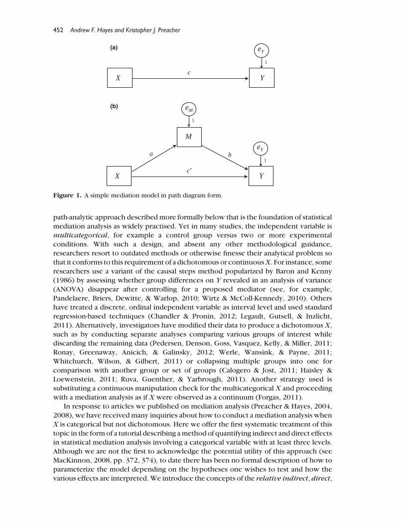
The simple mediation model, the focus of this paper, is diagrammed in Figure 1(b).

This model reflects a causal sequence in which X affects Y indirectly through mediator

variable M. In this model, X is postulated to affect M, and this effect then propagates

causally toY. This indirect effect represents themechanismbywhichX transmits its effecton Y. According to this model, X can also affect Y directly – the direct effect of X –independent of X’s influence onM. Examples of such a model are found in abundance in

psychological science (see Bearden, Feinstein, & Cohen, 2012; Johnson & Fujita, 2012).

The literature on statisticalmediation analysis focuses predominantly onmodelswith a

dichotomous or continuous independent variable, for this is a requirement of the

*Correspondence should be addressed to Andrew F. Hayes, Department of Psychology, The Ohio StateUniversity, Columbus, Ohio 43210, USA (email: [email protected]).

DOI:10.1111/bmsp.12028

451

path-analytic approach describedmore formally below that is the foundation of statistical

mediation analysis as widely practised. Yet in many studies, the independent variable ismulticategorical, for example a control group versus two or more experimental

conditions. With such a design, and absent any other methodological guidance,

researchers resort to outdated methods or otherwise finesse their analytical problem so

that it conforms to this requirement of a dichotomous or continuousX. For instance, some

researchers use a variant of the causal steps method popularized by Baron and Kenny

(1986) by assessing whether group differences on Y revealed in an analysis of variance

(ANOVA) disappear after controlling for a proposed mediator (see, for example,

Pandelaere, Briers, Dewitte, & Warlop, 2010; Wirtz & McColl-Kennedy, 2010). Othershave treated a discrete, ordinal independent variable as interval level and used standard

regression-based techniques (Chandler & Pronin, 2012; Legault, Gutsell, & Inzlicht,

2011). Alternatively, investigators have modified their data to produce a dichotomous X,

such as by conducting separate analyses comparing various groups of interest while

discarding the remaining data (Pedersen, Denson, Goss, Vasquez, Kelly, & Miller, 2011;

Ronay, Greenaway, Anicich, & Galinsky, 2012; Werle, Wansink, & Payne, 2011;

Whitchurch, Wilson, & Gilbert, 2011) or collapsing multiple groups into one for

comparison with another group or set of groups (Calogero & Jost, 2011; Haisley &Loewenstein, 2011; Ruva, Guenther, & Yarbrough, 2011). Another strategy used is

substituting a continuous manipulation check for the multicategorical X and proceeding

with a mediation analysis as if X were observed as a continuum (Forgas, 2011).

In response to articles we published on mediation analysis (Preacher & Hayes, 2004,

2008), we have receivedmany inquiries about how to conduct a mediation analysis when

X is categorical but not dichotomous. Here we offer the first systematic treatment of this

topic in the formof a tutorial describing amethod of quantifying indirect and direct effects

in statistical mediation analysis involving a categorical variable with at least three levels.Although we are not the first to acknowledge the potential utility of this approach (see

MacKinnon, 2008, pp. 372, 374), to date there has been no formal description of how to

parameterize the model depending on the hypotheses one wishes to test and how the

various effects are interpreted.We introduce the concepts of the relative indirect, direct,

M

YX

ba

eM

eY

1

1

c'

YX

eY

1

c

(a)

(b)

Figure 1. A simple mediation model in path diagram form.

452 Andrew F. Hayes and Kristopher J. Preacher

and total effect and illustrate how they are estimated and interpreted. Following this, we

describe inferential tests of relative effects. Woven throughout are the results of the

application of this approach using SPSS, SAS, and Mplus code documented in an online

supplement (Appendix S1). Our goal in this paper is to illustrate some ways that groupscould be represented in amediationmodel and the consequences of the choice on how to

interpret the effects that result, while also providing researchers with a means of

implementing this approach using popular software.

At the outset, it is important to note that we do not offer a means of assessing cause.

Mediation is a causal phenomenon, but no statistical model can prove causality. Causality

is established by appropriate research design and logical or theoretical argument.

Statistics can be used to ascertain whether an association between variables exists and of

what magnitude. This may aid in establishing the soundness of the causal argument, butdoes not prove it. Yet a statistical model can be used to eliminate certain alternative

explanations, and more complex statistical approaches than we discuss here can be used

in non-experimental studieswhen causal inference is less justified due to limitations of the

design (such as non-random assignment; see, for example, Hong, 2012; Muth�en, 2011;Pearl, 2012). Causal inference can be strengthened if the researcher can argue or

demonstrate that the variables are modelled in the appropriate causal sequence, if key

effects in a mediation model are not confounded by omitted variables (Imai, Keele, &

Tingley, 2010; Imai, Keele, &Yamamoto, 2010), and if no importantmoderation effects gounmodelled (Muller, Yzerbyt, & Judd, 2008; Pearl, 2012; VanderWeele & Vansteelandt,

2009, 2010; Yzerbyt, Muller, & Judd, 2004). For the purposes of this tutorial, we assume

that the user of the approachwe describe is comfortablewith causal claims beingmade or

acknowledges when non-causal interpretations exist and couches those claims appro-

priately given limitations of the data collection method.

1.1. Working exampleOur example is based on data provided by Kalyanaraman and Sundar (2006) from an

experiment on web portal customization and its effects on users. They proposed that

users of a more customized portal would have a more positive attitude toward the portal

than those using a less customized portal. They offer various potential mechanisms to

explain this effect. We focus here on perceived interactivity, a construct receiving much

attention in research on human–computer interaction. Kalyanaraman and Sundar

reasoned that people feel a customized web portal is more interactive, which translates

into a more favourable attitude toward the portal. Thus, they argue that customizationinfluences attitudes at least partly through perceived interactivity.

Sixty participants browsed theweb using a MyYahoo!web portal. Prior to arriving at a

computer laboratory, participants completed a questionnaire to assess their hobbies,

travel interests, favourite sports teams, preferred news sources, and so forth. This

information was used to construct a customized web portal for each participant through

which they would browse the web during the study. Participants assigned to the high

customization condition (n = 20) browsed the web using a portal that was highly

customized based on many of their responses to the pretest questionnaire (links to theirfavourite news pages, reviews of movies they might like, etc.). Participants in the

moderate customization condition (n = 20) browsed through a portal that had been

moderately customized, using fewer responses to the pretest questionnaire. Participants

assigned to the control condition (n = 20) browsed using a portal that had not been

customized at all. After a period of web browsing, their attitude toward the portal was

Mediation analysis with a multicategorical IV 453

assessed (with higher scores reflecting amore positive attitude) aswere their perceptions

of how interactive they believed the portal to be. Perceived interactivity was assessed

using a set of questions designed to measure the extent to which the users perceived the

portal as responsive to them and afforded a back-and-forth exchange of information, with

higher scores reflecting greater perceived interactivity.Descriptive statistics can be found in Table 1. A single-factor ANOVA on the attitude

measure reveals the expected effect of customization, F(2, 57) = 28.521, p < .001.

Pairwise comparisons betweenmeans reveal that those assigned to the highly customized

portal ð �Yhigh ¼ 7:300Þ had a significantly more positive attitude on average than those

assigned to the moderately customized portal ð �Ymoderate ¼ 6:005Þ as well as the control

condition ð �Ylow ¼ 4:335Þ. Furthermore, those assigned to the moderately customized

portal had a more positive attitude to the portal on average than those assigned to the

control condition. Thus, it seems attitudes were affected by customization. Whetherperceived interactivity is one of the mechanisms driving this effect will be addressed

throughout this tutorial.

2. Indirect, direct, and total effects

Figure 1 depicts a mediation model with a single mediator M through which X exertsits effect on Y. If M and Y are treated as continuous, X is either dichotomous or treated

as continuous, and all effects are linear, then the various effects (c0, a, and b in

Figure 1(b)) can be estimated with a set of ordinary least squares (OLS) regressions or

simultaneously using a structural equation modelling (SEM) program. Two linear

models are required:

M ¼ i1 þ aX þ eM ; ð1Þ

Y ¼ i2 þ c0X þ bM þ eY : ð2Þ

Of interest are the indirecteffectofX, quantifiedas theproductofaandb, and thedirect

effect, quantified as c0. The indirect effect, ab, is interpreted as the amount by which two

cases thatdifferbyoneunitonXareestimated todifferonYas a resultof theeffectofXonMwhich in turn affects Y. It serves as a quantitative instantiation of the mechanism through

whichX influencesY. Thedirect effectofXquantifies howmuch twocases equal onMbut

differing by one unit on X are estimated to differ on Y. It quantifies how differences in X

relate to differences in Y independent of M’s influence on Y. The total effect of X on Y,

Table 1. Descriptive statistics for the web portal customization study

Perceived

interactivity (M) Attitude (Y)

�M SD �Y SD �Y�

Control (n = 20) 4.250 1.839 4.335 1.647 4.792

Moderate (n = 20) 5.825 1.558 6.005 1.159 5.897

High (n = 20) 6.500 1.298 7.300 0.770 6.950

All groups combined 5.525 1.821 5.880 1.731 5.880

�Y� = adjusted mean, adjusted to the sample mean of perceived interactivity.


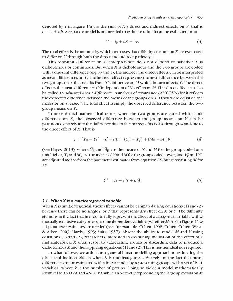
denoted by c in Figure 1(a), is the sum of X’s direct and indirect effects on Y, that is

c = c0 + ab. A separate model is not needed to estimate c, but it can be estimated from

Y ¼ i3 þ cX þ eY : ð3Þ

The total effect is the amount bywhich two cases that differ by one unit onX are estimated

to differ on Y through both the direct and indirect pathways.

This ‘one-unit difference on X’ interpretation does not depend on whether X is

dichotomous or continuous. But when X is dichotomous and the two groups are coded

with a one-unit difference (e.g., 0 and 1), the indirect and direct effects can be interpreted

asmean differences onY. The indirect effect represents themean difference between the

two groups on Y that results from X’s influence onMwhich in turn affects Y. The direct

effect is themeandifference inY independent ofX’s effect onM.This direct effect can alsobe called an adjusted mean difference in analysis of covariance (ANCOVA) for it reflects

the expected difference between the means of the groups on Y if they were equal on the

mediator on average. The total effect is simply the observed difference between the two

group means on Y.

In more formal mathematical terms, when the two groups are coded with a unit

difference on X, the observed difference between the group means on Y can be

partitioned entirely into the difference due to the indirect effect ofX throughM and due to

the direct effect of X. That is,

c ¼ ð �YH � �YLÞ ¼ c0 þ ab ¼ ð �Y �H � �Y �

L Þ þ ð �MH � �MLÞb; ð4Þ

(see Hayes, 2013), where �YH and �MH are the means of Y and M for the group coded one

unit higher, �YL and �ML are themeans ofY andM for the group coded lower, and �Y �H and �Y �

L

are adjustedmeans from the parameter estimates from equation (2) but substituting �M for

M:

�Y � ¼ i2 þ c0X þ b �M: ð5Þ

2.1. When X is a multicategorical variable

When X is multicategorical, these effects cannot be estimated using equations (1) and (2)

because there can be no single a or c0 that represents X’s effect onM or Y. The difficulty

stems from the fact that in order to fully represent the effect of a categorical variablewithk

mutually exclusive categories on somedependent variable (whetherMorY in Figure 1),k– 1 parameter estimates are needed (see, for example, Cohen, 1968; Cohen, Cohen,West,

& Aiken, 2003; Hardy, 1993; Suits, 1957). Absent the ability to model M and Y using

equations (1) and (2), researchers interested in examining mediation of the effect of a

multicategorical X often resort to aggregating groups or discarding data to produce a

dichotomousX and then applying equations (1) and (2). This is neither ideal nor required.

In what follows, we articulate a general linear modelling approach to estimating the

direct and indirect effects when X is multicategorical. We rely on the fact that mean

differences can be estimatedwith a linearmodel by representing groupswith a set of k – 1variables, where k is the number of groups. Doing so yields a model mathematically

identical to ANOVA and ANCOVAwhile also exactly reproducing the k groupmeans onM


and Y (both unadjusted and adjusted for group differences onM). As a consequence, the

model, parameter estimates, and model fit statistics (such as R2) retain all the information

about how thek groups differ fromeachother, unlikewhengroups are collapsed to form a

single dichotomous variable. It also allows for simultaneous hypothesis tests if the groupsare represented using carefully selected group codes to represent comparisons of interest.

There are many coding strategies that can be used to represent the groups. We first

illustrate the analysis using indicator coding, also known as dummy coding. To

dummy-code k groups, k – 1 dummy variables (Di, i = 1,…, k – 1) are constructed, with

Di set to 1 if a case is in group i, and 0 otherwise. One group is not explicitly coded,

meaning all k – 1 dummy variables are set to 0 for cases in that group. This group functions

as the reference category in the analysis, and parameters in the model pertinent to group

differences are quantifications relative to this reference group. Using these codes for X,the mediation model is parameterized with two equations, one for M and one for Y:

M ¼ i1 þ a1D1 þ a2D2 þ . . .þ ak�1Dk�1 þ eM ; ð6Þ

Y ¼ i2 þ c01D1 þ c02D2 þ . . .þ c0k�1Dk�1 þ bM þ eY ; ð7Þ

and represented in path diagram form in Figure 2(b). As in mediation analysis with acontinuous or dichotomous X, these models can be estimated separately as an OLS

regression-based path analysis or simultaneously using SEM.

Estimation of these models yields k – 1 a-coefficients quantifying differences between

the groups onM,k –1 c0-coefficients quantifying differences between groups onYholding

M constant, and a single b estimating the effect ofM on Ywhile statistically equating the

groups on average onX. The direct effect of X on Y is captured in the k – 1 estimates of c0ifrom equation (7), and the indirect effect of X on Y through M is estimated by the k – 1

products aib, i = 1,…, k – 1, from equations (6) and (7).We adopt the terms relative indirect effect and relative direct effect to refer to aib and

c0i, respectively. Of course, effects in virtually any analysis can be thought of as relative to

some alternative condition or state of affairs. Our decision to label these effects relative

formally acknowledges that the direct and indirect effects resulting from the analysis

described here will depend on how the independent variable is coded even though the

data being analysed are otherwise the same. But regardless of the choice, they will always

quantify the effect of being in one group (or set of groups) relative to some reference

group or set of groups. For example, in a simple dummy coding system, as in this example,aib is the indirect effect on Y viaM of being in group i relative to the reference group, and

c0i represents the direct effect of being in group i on Y relative to the reference group.

A different choice of reference group will result in different relative effects.

WhenX is multicategorical, there is no one parameter estimate that can be interpreted

as the total effect of X. Rather, the total effect is quantified with a set of k – 1 parameter

estimates resulting from the estimation ofY from the k – 1dummyvariables coding groups

in a linear model (see Figure 2(a)):

Y ¼ i3 þ c1D1 þ c2D2 þ . . .þ ck�1Dk�1 þ eY : ð8Þ

In equation (8) the k – 1 estimates of ci, i = 1,…,k, quantifymean differences between the

groups on Y. We refer to these k – 1 estimates as relative total effects. In the case of

indicator coding, ci quantifies the mean difference in Y between the group coded withDi


and the reference group. Regardless of the system used for coding groups, the relative

total effects are equal to the sum of the corresponding relative direct and indirect effects:

ci ¼ c0i þ aib: ð9Þ

2.2. Example

We illustrate the computation of the relative indirect, direct, and total effects using the

web browsing data and the indicator coding system described above and the inset of

Figure 3(a). D1 codes the moderate customization condition, D2 codes the high

customization condition, and the control group functions as the reference group and

receives a code of 0 on D1 and D2.

The coefficients in equations (6), (7), and – optionally – (8) can be estimated using anysoftware capable of estimating a linear model, whether an OLS regression program

commonly used by social scientists such as SPSS or SAS, or specialized SEM software such

as Mplus, LISREL, or AMOS using maximum likelihood (ML) estimation. Parameter

estimates will not be affected by the choice of OLS or ML estimation, but the standard

M

Y

D1

Dk-1

b

c1'a k-2

a1

eM

eY

1

1

ck-2'

Dk-2

.

.

.

a k-1 ck-1'

Y

D1

Dk-1

c1

eY

1

ck-2

Dk-2

.

.

.

ck-1

(a)

(b)

Figure 2. A mediation model in path diagram form corresponding to a model with a multicate-

gorical independent variable with k categories.


errors will differ in smaller samples. This difference dissipates as sample size increases.

With the exception of Mplus, most programs do not offer options for generating

inferential tests for relative indirect effects discussed later. In the online supplement, weprovide Mplus code that yields the regression coefficients in Table 2. Those more

comfortable in an OLS regression environment can use the PROCESS or MEDIATEmacros

for SPSS and SAS (see Hayes, 2013) also described in the online supplement.

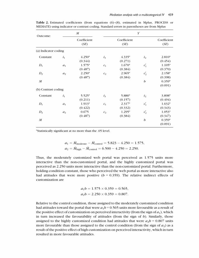
Estimating equations (6), (7), and (8) yields i1= 4.250, i2 = 2.810, i3 = 4.335, a1 = 1.575,a2 = 2.250, b = 0.359, c01 ¼ 1:105, c02 ¼ 2:158, c01 ¼ 1:670, and c01 ¼ 2:965 (see Table 2 or

Figure 3(a)). As can be seen by comparing the group statistics in Table 1 to their

derivation from themodel coefficients in Tables 2 and 3, themodels reproduce the group

means on M as well as the adjusted and unadjusted group means on Y.The relative indirect effects ofX onY throughM are constructed bymultiplyinga1 and

a2 by b. In this model, a1 and a2 correspond to the mean differences in perceived

interactivity between the moderately and highly customized conditions, respectively,

relative to the control condition:

M

Y

D1

D2

b = 0.359a1 = 1.575

eM

eY

1

1

c = 2.1582'

PerceivedInteractivity

Attitude

a2 = 2.250

c = 1.1051'

M

Y

D1

D2

b = 0.359a1 = 1.913

eM

eY

1

1

c = 1.0532'

PerceivedInteractivity

Attitude

a2 = 0.675

c = 1.6321'

Control Moderate High

D1 0 1 0

D2 0 0 1

Control Moderate High

D1 –0.667 0.333 0.333

D2

Indicator coding

Contrast coding

–0.5000 0.500

(a)

(b)

Figure 3. Estimated model coefficients resulting from (a) indicator coding and (b) a specific set of

contrast codes for customization condition.


a1 ¼ �Mmoderate � �Mcontrol ¼ 5:823� 4:250 ¼ 1:575;

a2 ¼ �Mhigh � �Mcontrol ¼ 6:500� 4:250 ¼ 2:250:

Thus, the moderately customized web portal was perceived as 1.575 units more

interactive than the non-customized portal, and the highly customized portal was

perceived as 2.250 units more interactive than the non-customized portal. Furthermore,

holding condition constant, those who perceived the web portal as more interactive alsohad attitudes that were more positive (b = 0.359). The relative indirect effects of

customization are

a1b ¼ 1:575� 0:359 ¼ 0:565;

a2b ¼ 2:250� 0:359 ¼ 0:807:

Relative to the control condition, those assigned to the moderately customized conditionhad attitudes toward the portal that were a1b = 0.565 units more favourable as a result of

the positive effect of customization on perceived interactivity (from the sign of a1), which

in turn increased the favourability of attitudes (from the sign of b). Similarly, those

assigned to the highly customized condition had attitudes that were a2b = 0.807 units

more favourable than those assigned to the control condition (from the sign of a2) as a

result of the positive effect of high customization on perceived interactivity, which in turn

resulted in more favourable attitudes.

Table 2. Estimated coefficients (from equations (6)–(8), estimated in Mplus, PROCESS or

MEDIATE) using indicator or contrast coding. Standard errors in parentheses are from Mplus

Outcome:M Y

Coefficient

(SE)

Coefficient

(SE)

Coefficient

(SE)

(a) Indicator coding

Constant i1 4.250* i3 4.335* i2 2.810*

(0.344) (0.271) (0.454)

D1 a1 1.575* c1 1.670* c01 1.105*

(0.487) (0.384) (0.370)

D2 a2 2.250* c2 2.965* c02 2.158*

(0.487) (0.384) (0.398)

M b 0.359*

(0.091)

(b) Contrast coding

Constant i1 5.525* i3 5.880* i2 3.898*

(0.211) (0.157) (0.494)

D1 a1 1.913* c1 2.317* c01 1.632*

(0.422) (0.332) (0.343)

D2 a2 0.675 c2 1.295* c02 1.053*

(0.487) (0.384) (0.347)

M b 0.359*

(0.091)

*Statistically significant at no more than the .05 level.


Table

3.Derivationofgroupmean

sfrom

themodelcoefficients

Condition

Indicatorcodingexam

ple

Contrastcodingexam

ple

� M=i 1+a1D1+a2D2

=i 1+a1D1+a2D2

Control

4.250

=4.250+1.575(0)+2.225(0)

=5.525+1.913(–0.667)+0.675(0)

Moderate

5.825

=4.250+1.575(1)+2.225(0)

=5.525+1.913(0.333)+0.675(–0.5)

High

6.500

=4.250+1.575(0)+2.225(0)

=5.525+1.913(0.333)+0.675(0.5)

� Y�

=i 2+c0 1D1+c0 2D2+bM

=i 2+c0 1D1+c0 2D2+bM

Control

4.793

=2.810+1.105(0)+2.158(0)+0.359(5.525)

=3.898+1.631(–0.667)+1.053(0)+0.359(5.525)

Moderate

5.897

=2.810+1.105(1)+2.158(0)+0.359(5.525)

=3.898+1.631(0.333)+1.053(–0.5)+0.359(5.525)

High

6.950

=2.810+1.105(0)+2.158(1)+0.359(5.525)

=3.898+1.631(0.333)+1.053(0.5)+0.359(5.525)

� Y=i 3+c 1D1+c 2D2

=i 3+c 1D1+c 2D2

Control

4.335

=4.335+1.670(0)+2.965(0)

=5.880+2.317(0.667)+1.295(0)

Moderate

6.005

=4.335+1.670(1)+2.965(0)

=5.880+2.317(0.333)+1.295(–0.5)

High

7.300

=4.335+1.670(0)+2.965(1)

=5.888+2.317(0.333)+1.295(0.5)


In equation (7), c01 and c02 are the relative direct effects of moderate and high

customization, respectively, relative to the control condition, and quantify the corre-

sponding differences between adjustedmeans ( �Y �) on the attitudemeasure (see Table 1):

c01 ¼ �Y �moderate � �Y �

control ¼ 5:897� 4:792 ¼ 1:105;

c02 ¼ �Y �high � �Y �

control ¼ 6:950� 4:792 ¼ 2:158:

Adjusting for group differences in perceived interactivity, those who browsed using a

moderately customized web portal reported attitudes that were 1.105 units more

favourable than those who browsed using a non-customized portal, and those who

browsed with a highly customized portal had attitudes 2.157 units more favourable than

those who browsed using a non-customized portal.

The relative total effects, c1 and c2, can be found in Table 2. These are equivalent to the

mean difference in attitudes between the moderate and high customization conditions

relative to the control condition, respectively:

c1 ¼ �Ymoderate � �Ycontrol ¼ 6:005� 4:335 ¼ 1:670;

c2 ¼ �Yhigh � �Ycontrol ¼ 7:300� 4:335 ¼ 2:965:

These relative total effects can also be calculated by adding the corresponding relative

direct and indirect effects c1 ¼ c01 þ a1b ¼ 1:105þ 0:565 ¼ 1:670, and c2 ¼ c02 þ a2b ¼2:158þ 0:807 ¼ 2:965.

The relative total, direct, and indirect effects calculated above are all scaled as mean

differences in ametric ofY that, in this example, is arbitrary. Dividing each of these effects

by the standard deviation of Y (or standardizing Y prior to analysis) results in effects that

can be interpreted as a standardized mean difference analogous to Cohen’s d, and

equation (9) still holds. Even so, a standardized versionof an arbitrary scale is still arbitrary;

standardized effect sizemeasures are not necessarily anymoremeaningful theoretically or

practically than unstandardized measures, and unstandardized effects can be meaningful

if the scaling is inherently meaningful or widely used in a research area (see Preacher &Kelley, 2011). Expressing a relative direct or indirect effect as a ratio relative to its

corresponding relative total effect,while tempting, has documented problems as an effect

size measure and so we discourage doing so. The quantification and interpretation of

effect size are an evolving and controversial topic in statistical mediation analysis and

elsewhere. Moreover, whether an effect can be deemed large or small is not entirely a

statistical question. See Hayes (2013), Kelley and Preacher (2012), and Preacher and

Kelley (2011) for a discussion of various measures and controversies.

3. Statistical inference

Statistical inference for the total and direct effects of X is straightforward and

uncontroversial. For relative direct and total effects, all regression routines programmed

into statistical packages that are widely used, as well as most SEM programs, provide

standard errors for these effects for testing the null hypothesis of no relative effect usinglevel of significance a. Alternatively, 100(1 – a)% confidence intervals (CI) can be

constructed as the point estimate plus orminus ta/2 standard errors, where ta/2 is the value

of t that cuts off the upper and lower 100(a/2)%of the t(df) distribution from the rest of the


distribution, with degrees of freedom (df) equal to the residual degrees of freedom in the

models of Y (i.e., equations (7) and (8)).1

Using the indicator coding strategy, as can be seen in Table 2, all relative direct and

total effects in the web browsing analysis are positive and statistically different from zerofor all comparisons (D1, moderate customization versus control; D2, high customization

versus control). Regardless of whether or not perceived interactivity is controlled,

customization seems to engender more favourable attitudes to the portal.

3.1. Inference for relative indirect effects

Until recently, the causal steps approach dominated the practice of statistical mediation

analysis. This approach focuses on estimating each of the pathways in the model inFigure 1 and then conducting significance tests for each of the effects while qualitatively

comparing the size of the direct effect and total effect ofX. If certain criteria are met, then

it can be said thatMmediates the effect of X on Y. A formal statistical test of the indirect

effect is not required by this approach. Rather, its existence is inferred logically through

the rejection of various null hypotheses about the individual paths and the size of the

direct relative to the total effect of X.

This causal steps approach can be and has been used when X is a multicategorical

variable. But for reasons already documented in the mediation analysis literature (seeHayes, 2009, 2013; Rucker, Preacher, Tormala, & Petty, 2011), we advise researchers to

eschew methods that rely on testing components of the indirect effect (i.e., ai and b) in

favour of a formal inferential test of the product of ai and b. Evidence that at least one

relative indirect effect is different from zero supports the conclusion thatMmediates the

effect of X on Y.

Of the many methods one could use for statistical inference about relative indirect

effects (see MacKinnon, Lockwood, Hoffman, West, & Sheets, 2002; MacKinnon,

Lockwood, & Williams, 2004), we advocate the asymmetric bootstrap CI. We prefer thismethod because it does not make the unwarranted assumption of normality of the

sampling distribution of the relative indirect effect, it performs well as evidenced in

numerous simulation studies (Biesanz, Falk, & Savalei, 2010; Hayes & Scharkow, 2013;

MacKinnon et al., 2004; Williams & MacKinnon, 2008), and it is easy to implement in

existing software such as Mplus, SPSS, and SAS using the code provided in the online

supplement.

A percentile bootstrap CI for a relative indirect effect is constructed by repeatedly

taking samples of size n with replacement from cases in the data (e.g., participants inthe study), where n is the size of the original sample, and estimating all the coefficients

in the mediation model using equations (6) and (7) in each bootstrap sample. From the

estimated coefficients, the relative indirect effects are calculated. Repeated j times

(ideally j = 5,000 or more), the distributions of j relative indirect effects serve as

empirical approximations of their sampling distributions. A 100(1 – a)% CI for each

relative indirect effect is constructed as the bootstrap estimates that define the lower

and upper 100(a/2)% of the distribution of j estimates, respectively. The relative

indirect effect is deemed statistically different from zero if the CI does not straddlezero.

1 An omnibus test of the total and direct effects of X could be conducted using the F-ratio with k – 1 and dferrordegrees of freedom from an ANOVA or ANCOVA respectively, or from corresponding regression statistics.


Adjustments to the CI endpoints have been offered to produce the bias-corrected or

bias-corrected and accelerated bootstrap CI (see Efron & Tibshirani, 1993). There is

some evidence that the percentile bootstrap method is preferable in some circum-

stances, as the bias-corrected methods have a slightly inflated Type I error rate whenone of the two paths in the mediation process is zero (see Fritz, Taylor, & MacKinnon,

2012; Hayes & Scharkow, 2013). Otherwise, the bias-corrected bootstrap CI is more

powerful.2

Using indicator coding with the control group as the reference group and with the aid

of SPSS, SAS, or Mplus code in the online supplement yields 95% bias-corrected bootstrap

CIs for the relative indirect effects that do not straddle zero (based on 10,000 bootstrap

samples), indicating that both customization conditions (relative to the control

condition) indirectly influence attitudes through perceived interactivity (moderatecustomization, 95% CI = 0.169 to 1.255; high customization, 95% CI = 0.334 to 1.659).

This supports a claim that perceived interactivity functions as a mediator of the effect of

customization on attitudes. Historically, this result would be described as ‘partial

mediation’ because the corresponding relative total and direct effects of customization

are both statistically different from zero. But this term (along with ‘complete mediation’)

has recently been heavily criticized. For reasons discussed in Hayes (2013) and Rucker

et al. (2011), we recommend not couching the interpretation of the indirect effect in

such terms that rely on the outcome of tests of significance of the relative direct or totaleffects.3

3.2. Multiple test correction

WhenX is amulticategorical variable, the number of possible tests one could conduct in a

mediation analysis as described above can be large, and we encourage researchers to be

mindful of the problems this can produce. A researcher concerned about Type I error

inflation resulting from reliance on several inferential tests of relative effects could chooseto adjust p-values or base inferences on CIs greater than 95%. For instance, with a

three-level X and assuming independent adjustments for the sets of two relative direct,

indirect, and total effects, a Bonferroni approach tomultiple test correctionwould involve

the use of a p-value criterion of .025 for rejection of a null hypothesis or a 97.5% CI that

does not straddle zero before claiming that a relative effect is different from zero. Doing so

in the example above does not change the results or their substantive interpretation. A

more (or less) conservative adjustment could be employed depending on the number of

tests being conducted in the analysis overall, disciplinary norms, or one’s beliefs about therelative risks and costs of Type I relative to Type II errors.

2 In principle, bootstrap CIs could be used for inference about relative and total direct effects. But there is littlestatistical advantage to doing so because, unlike the relative indirect effect, the sampling distributions of theseeffects are typically normal or nearly so.3 There is a limitation of this approach tomediation analysis that is important to acknowledge. Because estimatesof relative indirect effects will depend on the coding used to represent groups, it is conceivable that one couldfind evidence of mediation of X’s effect on Y byM for one coding choice but not for another, depending on thesizes of the indirect effects relative to the reference group. We have proposed an inferential test of the omnibus

indirect effect that we believe overcomes this limitation, but it is still being evaluated. See the documentation forMEDIATE at www.afhayes.com for a definition and discussion.


4. Alternative coding systems

Indicator coding is not the only system for representing groups. Which coding system touse will be guided by specific questions the investigator wants to answer, and the choice

will influence how the relative indirect, direct, and total effects are interpreted. Belowwe

illustrate the computation and interpretation of these effects using one alternative:

unweighted contrast coding.

To illustrate this approach,we constructed k –1 variables (two in this case) coding two

contrasts, one corresponding to the control condition relative to the two customization

conditions combined, and the second comparing to the two customization conditions.

Using well-disseminated rules for the construction of contrasts (see, for example, Keppel& Wickens, 2004; Rosenthal & Rosnow, 1985), the codes corresponding to the first

contrast are –2, 1, and 1 for the control, moderate, and high conditions, respectively. For

the second contrast the codes are 0, –1, and 1. Even if only one contrast is of substantive

interest, it is still important that the additional k – 2 sets of contrast codes be specified andincluded in the models of Y and M. Failure to do so will yield a model that does not

reproduce the group means.

Although not mathematically necessary, we recommend a transformation of the

contrast codes so that the largest and smallest codes in a set differ by only one unit. Thisscales all relative direct, indirect, and total effects on a mean difference metric (see, for

example, West, Aiken, & Krull, 1996). This is accomplished by dividing each of the

codes in the k – 1 sets by the absolute value of the difference between the largest and

smallest contrast codes in the set. For example, the first set contains three codes (–2, 1,1) the largest and smallest which differ by 3 units, and the second set contains codes

with a maximum absolute difference of 2. Thus, the resulting transformed codes become

–2/3, 1/3, and 1/3 for the first set and 0, –1/2, and 1/2 for the second set. Therefore, D1

andD2 are defined for each condition as D1 = –0.667, D2 = 0 for control, D1 = 0.333, D2 =–0.5 for moderate customization, D1 = 0.333, D2 = 0.5 for high customization (see

Figure 3(b)).

With D1 and D2 constructed in this manner, estimation of the coefficients in

equations (6)–(8) yields i1 = 5.525, i2 = 3.898, i3 = 5.880, a1 = 1.913, p < .001; a2 =0.675, p = .166; b = 0.359, p < .001, c01 ¼ 1:631; p < .001; and c02 ¼ 1:053, p = .002;

c1 = 2.317, p < .001; c2 = 1.295, p < .002 (see Table 2). Comparing the statistics in

Table 1 to their derivation from the model coefficients in Tables 2 and 3 verifies that

the resulting models reproduce the group means on M as well as the adjusted andunadjusted group means on Y.

The relative indirect effects are estimated as products of coefficients just as when

indicator coding is used, and the SPSS and SAS macros or Mplus code described in the

online supplement can be used to generate bootstrap CIs for inference. The relative

indirect effect for the first contrast comparing any customization to the control condition

is the contrast for perceived interactivity,

a1 ¼�Mmoderate þ �Mhigh

2� �Mcontrol

¼ 5:825þ 6:500

2� 4:250 ¼ 1:913;

multiplied by the effect of interactivity on attitudes independent of customization

condition, b = 0.359:


a1b ¼ 1:913� 0:359 ¼ 0:687:

Any customization results in amore favourable attitude by 0.687 units as a result of greater

perceptions of interactivity in the customized portals (from the sign of a1), which in turnleads to a more favourable attitude (from the sign of b). A 95% bias-corrected bootstrap CI

for this relative indirect effect is from0.259 to 1.387. This relative indirect effect is positive

and statistically different from zero.

The relative indirect effect for the second contrast corresponds to the effect of high

versus moderate customization on attitudes through perceived interactivity. The contrast

for perceived interactivity corresponds to the difference in mean perceived interactivity

between the high and moderate customization conditions,

a2 ¼ �Mhigh � �Mmoderate ¼ 6:500� 5:825 ¼ 0:675:

When multiplied by the effect of perceived interactivity on attitudes (b), the result is the

relative indirect effect of high versus moderate customization on attitudes,

a2b ¼ 0:675� 0:359 ¼ 0:242:

High customization yields attitudes that are 0.242 units more favourable on average

relative to moderate customization due to the greater perceptions of interactivity that

result from more customization (from the sign of a2), which in turn positively

influences attitudes (from the sign of b). But a 95% bias-corrected bootstrap CI for

this relative indirect effect straddles zero (from –0.033 to 0.720). Thus, the evidence isnot sufficiently strong to claim an indirect effect of high relative to moderate

customization.4

The relative direct effect c01 corresponds to the effect ofany customization on attitudes

relative to none, independent of perceived interactivity. The relative direct effect c02 is theeffect of high relative to moderate customization on attitudes independent of perceived

interactivity. These relative direct effects correspond to differences between adjusted

means, in the former case an unweighted combination of the means in the two

customization conditions:

c01 ¼�Y �moderate þ �Y �

high

2� �Y �

control

¼ 5:897þ 6:950

2� 4:792 ¼ 1:632;

c02 ¼ �Y �high � �Y �

moderate ¼ 6:950� 5:897 ¼ 1:053:

Independent of the effect of perceptions of interactivity on attitude, any customization

yields attitudes that are 1.632 units more favourable on average relative to no

customization. Furthermore, high customization yields attitudes that are 1.053 units

more favourable on average than moderate customization. Tests of significance available

in standard regression output or using the code described in the online supplement can beused for inference about these relative direct effects.

4 A Bonferroni correction of 2 applied to each set of tests does not change the results in this example.


The relative total effects, c1 and c2, are estimated using equation (8) or by adding the

corresponding relative direct and indirect effects. These relative total effects of

customization on attitudes quantify the mean difference in attitudes toward the portal

for any customization relative to none (c1) and high relative to moderate customization(c2):

c1 ¼�Ymoderate þ �Yhigh

2� �Ycontrol

¼ 6:005þ 7:300

2� 4:335 ¼ 2:317;

c2 ¼ �Yhigh � �Ymoderate ¼ 7:300� 6:005 ¼ 1:295:

Observe that these relative total effects partition into the relative direct and indirect

effects c1 ¼ c01 þ a1b ¼ 1:632þ 0:675 ¼ 2:317 and c2 ¼ c02 þ a2b ¼ 1:053þ 0:242 ¼1:295. Standard regression output contains inferential tests for these relative total effects.

Any coding system used in ANOVA could be applied to mediation analysis in this

fashion. For example, if the independent variable is discrete and ordinal, Helmert coding

could be used to estimate the relative effects of category j relative to the aggregate of all

ordinally higher levels. In the online supplement, we provide an illustration using

sequential coding, also useful for discrete, ordinal independent variables. For a discussion

of various coding strategies, see Cohen et al. (2003), Davis (2010), Hardy (1993),

Kaufman and Sweet (1974), Serlin and Levin (1985), Wendorf (2004), and West et al.

(1996).

5. Between-group heterogeneity in the effect ofM on Y

An assumption frequently described as necessary for causal inference in mediation

analysis is the no-interaction assumption or, in ANCOVA terms, homogeneity of

regression: the effect of M on Y is invariant across values of X. If this assumption is

violated, it is not sensible to estimate a relative indirect effect as aib because b in equation

(7) does not accurately characterize the association betweenM andY,which is contingent

on X and thus not a single number. Furthermore, interaction between X and M implies

that at least one relative direct effect depends on M.

This assumption can be tested by including interaction terms in the model ofY. This is

accomplished by respecifying the model of Y in equation (7) as

Y ¼ i2 þ c01D1 þ c02D2 þ . . .þ c0k�1Dk�1 þ b1D1M þ b2D2M þ . . .

þ bk�1Dk�1M þ bkM þ eY ;

ð10Þ

and testing the null hypothesis that all population bi, i = 1,…, k – 1, equal zero. Rejectionimplies that the effect of M on Y depends on X. When using OLS regression, this test is

implemented using hierarchical variable entry inwhichR2 from themodel in equation (7)

is subtracted from R2 from equation (10) to yield DR2. Under the null hypothesis of no

interaction, df(DR2)/[(1 � R2)(k � 1)] follows the F(k – 1, df) distribution, where df and

R2 are the residual degrees of freedom and squared multiple correlation, respectively,

from the model in equation (10). Alternatively, using SEM, the fit of two models can be

compared, one with all bi, i = 1,…, k – 1, constrained to be zero versus one with them

freely estimated. Under the null hypothesis of no interaction, the difference in v2 for the


twomodels follows thev2(k –1) distribution. If thep-value for this test is belowa, then theassumption of homogeneity of regression has been violated. The outcome of either test

will be invariant to the choice of coding system.

In this example, the difference in R2 between the two models of attitudes toward the

web portal (Y) with andwithout the k – 1 products representing the interaction between

web customization condition and perceived interactivity was DR2 = .004 and not

statistically significant, F(2,54) = .297, p = .744. Thus, the homogeneity of regression

assumption is not contradicted by the data. If the test instead suggested a violation of this

assumption, the relative direct and indirect effects calculated as described above will

mischaracterize the effect of X to a degree dependent on the size of the interaction.

This assumption of no interaction between X and M represents a special case of the

assumption that one’s model is properly specified. Because both X andM are available inthe data, this is easy to test and we recommend doing so. Yet in principle any of the paths

in a mediation model could be moderated by other variables, and a failure to include such

interactions potentially also represents a misspecification that is as important as the

assumption that X does not interact with M. It is routine for researchers to either ignore

such possibilities or empirically test for them. Principles described in the literature on

‘moderated mediation’ (Edwards & Lambert, 2007; Muller, Judd, & Yzerbyt, 2005;

Preacher, Rucker, & Hayes, 2007) could be extended to models with a multicategorical

independent variable, including the case whereX andM interact. How to do so is beyondthe scope of this tutorial.

6. Summary

In this tutorial, we have illustrated a method for estimating indirect, direct, and total

effects in statistical mediation analysis with a multicategorical independent variable.These relative effects quantify the effects of being in one category on some outcome

relative to some other group or set of groups used as a reference for comparison. The

outcome of tests of relative effects will be dependent on the choices one makes about

coding groups and which group or groups are used as the reference for comparison

purposes. Possible extensions to this method are abundant, and in an online supplement

we discuss confounding, random measurement error, multiple mediators, and an

additional example using sequential coding of groups. We hope this tutorial will facilitate

the implementation of this approach and enable researchers to apply the advice givenrecently bymethodologists who studymediation analysis to research designs that include

a multicategorical independent variable.

References

Baron, R. M., & Kenny, D. A. (1986). The moderator–mediator variable distinction in social

psychological research: Conceptual, strategic, and statistical considerations. Journal of

Personality and Social Psychology, 51, 1173–1182. doi:10.1037/0022-3514.51.6.1173Bearden, D. J., Feinstein, A., &Cohen, L. L. (2012). The influence of parent preprocedural anxiety on

child procedural pain: Mediation by child procedural anxiety. Journal of Pediatric Psychology,

37, 680–686. doi:10.1093/jpepsy/jss041Biesanz, J. C., Falk, C. F., & Savalei, V. (2010). Assessing meditational models: Testing and interval

estimation for indirect effects. Multivariate Behavioral Research, 45, 661–701. doi:10.1080/00273171.2010.498292


Bullock, J. G., Green,D. P., &Ha, S. E. (2010). Yes, butwhat is themechanism? (Don’t expect an easy

answer). Journal of Personality and Social Psychology, 98, 550–558. doi:10.1037/a0018933Calogero, R. M., & Jost, J. T. (2011). Self-subjugation among women: Exposure to sexist ideology,

self-objectification, and the protective function of the need to avoid closure. Journal of

Personality and Social Psychology, 100, 211–228. doi:10.1037/a0018933Chandler, J. J., & Pronin, E. (2012). Fast thought speed induces risk taking. Psychological Science,

23, 370–374. doi:10.1177/0956797611431464Cohen, J. (1968). Multiple regression as a general data-analytic system. Psychological Bulletin, 70,

426–443. doi:10.1037/h0026714Cohen, J., Cohen, P.,West, S. G., & Aiken, L. S. (2003).Appliedmultiple regression and correlation

analysis for the behavioral sciences (3rd ed.). New York, NY: Routledge.

Davis, M. J. (2010). Contrast coding in multiple regression analysis: Strengths, weaknesses, and

utility of popular coding structures. Journal of Data Science, 8, 61–73.Edwards, J. R., & Lambert, L. S. (2007).Methods for integratingmoderation andmediation: A general

analytical framework using moderated path analysis. Psychological Methods, 12, 1–22. doi:10.1037/1082-989X.12.1.1

Efron, B., & Tibshirani, R. J. (1993). An introduction to the bootstrap. New York, NY: Chapman &

Hall.

Forgas, J. P. (2011). Affective influences on self-disclosure: Mood effects on the intimacy and

reciprocity of disclosing personal information. Journal of Personality and Social Psychology,

100, 449–461. doi:10.1037/a0021129Fritz, M. S., Taylor, A. B., & MacKinnon, D. P. (2012). Explanation of two anomalous results in

statistical mediation analysis. Multivariate Behavioral Research, 47, 61–87. doi:10.1080/00273171.2012.640596

Haisley, E., & Loewenstein, G. (2011). It’s not what you get but when you get it: The effect of gift

sequence on deposit balances and customer sentiment in a commercial bank. Journal of

Marketing Research, 48, 103–115. doi:10.1509/jmkr.48.1.103

Hardy, M. A. (1993). Regression with dummy variables. Newbury Park, CA: Sage.

Hayes, A. F. (2009). Beyond Baron and Kenny: Statistical mediation analysis in the newmillennium.

Communication Monographs, 76, 408–420. doi:10.1080/03637750903310360Hayes, A. F. (2013).An introduction tomediation,moderation, and conditional process analysis:

A regression-based approach. New York, NY: Guilford Press.

Hayes, A. F., & Scharkow, M. (2013). The relative trustworthiness of tests of indirect effects in

statisticalmediation analysis. Doesmethod reallymatter?Psychological Science,24, 1918–1927.doi:10.1177/0956797613480187

Hong, G. (2012). Marginal mean weighting through stratification: A generalized method for

evaluating multivalued and multiple treatments with nonexperimental data. Psychological

Methods, 17, 44–60. doi:10.1037/a0024918Imai, K., Keele, L., & Tingley, D. (2010). A general approach to causal mediation analysis.

Psychological Methods, 15, 309–334. doi:10.1037/a0020761Imai, K., Keele, L., & Yamamoto, T. (2010). Identification, inference and sensitivity analysis for

causal mediation effects. Statistical Science, 25, 51–71. doi:10.1214/10-STS321Johnson, I. R., & Fujita, K. (2012). Change we can believe in: Using perceptions of changeability to

promote system-change motives over system-justification motives in information search.

Psychological Science, 22, 133–140. doi:10.1177/0956797611423670Kalyanaraman, S., & Sundar, S. S. (2006). The psychological appeal of personalized content in web

portals: Does customization affect attitudes andbehavior? Journal of Communication,31, 254–270. doi:10.1111/j.1460-2466.2006.00006.x

Kaufman, D., & Sweet, R. (1974). Contrast coding in least squares regression analysis. American

Educational Research Journal, 11, 359–377. doi:10.3102/00028312011004359Kelley, K., & Preacher, K. J. (2012). On effect size. Psychological Methods, 17, 137–152. doi:10.

1037/a0028086


Keppel, G., & Wickens, T. D. (2004). Design and analysis: A researcher’s handbook (4th ed.).

Upper Saddle River, NJ: Pearson Prentice Hall.

Legault, L., Gutsell, J. N., & Inzlicht, M. (2011). Ironic effects of antiprejudice messages: How

motivational interventions can reduce (but also increase) prejudice. Psychological Science, 22,

1472–1477. doi:10.1177/0956797611427918MacKinnon, D. P. (2008).An introduction to statisticalmediation analysis. NewYork: Routledge.

MacKinnon,D. P., Lockwood,C.M.,Hoffman, J.M.,West, S.G.,& Sheets, V. (2002). A comparison of

methods to test mediation and other intervening variable effects. Psychological Methods, 7, 83–103. doi:10.1037/1082-989X.7.1.83

MacKinnon, D. P., Lockwood, C. M., &Williams, J. (2004). Confidence limits for the indirect effect:

Distribution of the product and resampling methods. Multivariate Behavioral Research, 39,

41–62.doi:10.1207/s15327906mbr3901_4

Muller, D., Judd, C. M., & Yzerbyt, V. Y. (2005). When moderation is mediated and mediation is

moderated. Journal of Personality and Social Psychology, 89, 852–863. doi:10.1037/

0022-3514.89.6.852

Muller, D., Yzerbyt, V., & Judd, C. M. (2008). Adjusting for a mediator in models with two crossed

treatment variables. Organizational Research Methods, 11, 224–240. doi:10.1177/

1094428106296639

Muth�en, B. (2011). Applications of causally defined direct and indirect effects in mediation

analysis using SEM in Mplus. Manuscript submitted for publication.

Pandelaere, M., Briers, B., Dewitte, S., &Warlop, L. (2010). Better think before agreeing twice. Mere

agreement: A similarity-based persuasion mechanism. International Journal of Research in

Marketing, 27, 133–141. doi:10.1016/j.ijresmar.2010.01.003

Pearl, J. (2012). The causal mediation formula: A guide to the assessment of pathways and

mechanisms. Prevention Science, 13, 426–436. doi:10.1007/s11121-011-0270-1Pedersen, W. C., Denson, T. F., Goss, R. J., Vasquez, E. A., Kelley, N. J., & Miller, N. (2011). The

impact of rumination on aggressive thoughts, feelings, arousal, andbehaviour.British Journal of

Social Psychology, 50, 281–301. doi:10.1348/014466610X515696Preacher, K. J., & Hayes, A. F. (2004). SPSS and SAS procedures for estimating indirect effects in

simplemediationmodels.Behavior ResearchMethods, Instruments, and Computers, 36, 717–731. doi:10.3758/BF03206553

Preacher, K. J., & Hayes, A. F. (2008). Asymptotic and resampling strategies for assessing and

comparing indirect effects in multiple mediator models. Behavior Research Methods, 40, 879–891. doi:10.3758/BRM.40.3.879

Preacher, K. J., & Kelley, K. (2011). Effect size measures for mediation models: Quantitative

strategies for communicating indirect effects. PsychologicalMethods, 16, 93–115. doi:10.1037/a0022658

Preacher, K. J., Rucker, D. D., & Hayes, A. F. (2007). Assessing moderated mediation hypotheses:

Theory, methods, and prescriptions. Multivariate Behavioral Research, 42, 185–227. doi:10.1080/00273170701341316

Ronay, R., Greenaway, K., Anicich, E. M., & Galinsky, A. D. (2012). The path to glory is paved with

hierarchy: When hierarchical differentiation increases group effectiveness. Psychological

Science, 23, 669–677. doi:10.1177/0956797611433876Rosenthal, R., & Rosnow, R. L. (1985). Contrast analysis: Focused comparisons in the analysis of

variance. Cambridge, UK: Cambridge University Press.

Rucker, D. D., Preacher, K. J., Tormala, Z. L., & Petty, R. E. (2011). Mediation analysis in social

psychology: Current practices and new recommendations. Social and Personality Psychology

Compass, 5 (6), 359–371. doi:10.1111/j.1751-9004.2011.00355.xRuva, C. L., Guenther, C. C., & Yarbrough, A. (2011). Positive and negative pretrial publicity: The

roles of impression formation, emotion, and predecisional distortion. Criminal Justice and

Behavior, 38, 511–534. doi:10.1177/0093854811400823Serlin, R. C., & Levin, J. R. (1985). Teaching how to derive directly interpretable coding schemes for

multiple regression analysis. Journal of Educational Statistics, 10, 223–238.


Suits, D. B. (1957). Use of dummy variables in regression equations. Journal of the American

Statistical Association, 52, 548–551.VanderWeele, T. J., & Vansteelandt, S. (2009). Conceptual issues concerning mediation,

interventions and composition. Statistics and its Interface, 2, 457–468.VanderWeele, T. J., & Vansteelandt, S. (2010). Odds ratios for mediation analysis for a dichotomous

outcome. American Journal of Epidemiology, 172, 1339–1348. doi:10.1093/aje/kwq332

Wendorf, C. A. (2004). Primer onmultiple regression coding: Common forms and the additional case

of repeated contrasts. Understanding Statistics, 3, 47–57.Werle, C. O. C., Wansink, W., & Payne, C. R. (2011). Just thinking about exercise makes me serve

more food: Physical activity and calorie consumption. Appetite, 56, 332–335. doi:10.1016/j.appet.2010.12.016

West, S. G., Aiken, L. S., &Krull, J. L. (1996). Experimental personality designs: Analyzing categorical

by continuous variable interactions. Journal of Personality, 64, 1–48. doi:10.1111/j.1467-6494.1996.tb00813.x

Whitchurch, E. R., Wilson, T. D., & Gilbert, D. T. (2011). ‘He loves me, he loves me not…’:

Uncertainty can increase romantic attraction. Psychological Science, 22, 172–175. doi:10.1177/0956797610393745

Williams, J., & MacKinnon, D. P. (2008). Resampling and distribution of the product methods for

testing indirect effects in complex models. Structural Equation Modeling, 15, 23–51. doi:10.1080/10705510701758166

Wirtz, J., &McColl-Kennedy, J. R. (2010). Opportunistic customer claiming during service recovery.

Journal of the Academy of Marketing Science, 38, 654–675. doi:10.1007/s11747-009-0177-6Yzerbyt, V. Y., Muller, D., & Judd, C. M. (2004). Adjusting researchers’ approach to adjustment: On

the use of covariates when testing interactions. Journal of Experimental Social Psychology, 40,

424–431. doi:10.1016/j.jesp.2003.10.001

Received 22 April 2013; revised version received 2 September 2013

Supporting Information

The following supporting informationmay be found in the online edition of the article:

Appendix S1. Statistical mediation analysis with a multicategorical independent

variable


1

Online supplement to Hayes, A. F., & Preacher, K. J. (2014). Statistical mediation analysis with a multicategorical independent variable. British Journal of Mathematical and Statistical Psychology, 67, 451-470. DOI: 10.1111/bmsp.12028 [This document contains corrections to a few typos that were found on the version available through the journal’s web page and adds a note about new features in PROCESS that eliminate the need to run PROCESS twice] This document contains instructions for the implementation of the method described in Hayes and Preacher (2014) using Mplus as well as using the PROCESS and MEDIATE macros for SPSS and SAS. Following the code, various miscellaneous issues and extensions are addressed, including interpretation of model coefficients using sequential group coding, accounting for random measurement error, dealing with confounds statistically, and models with multiple mediators.

Mplus Code Corresponding to the Web Portal Customization Example

Any structural equation modeling program can produce estimates of the coefficients in a mediation model. Mplus offers features such as bootstrap confidence intervals for indirect effects and inferential tests for functions of parameters that make it a particularly good choice for the kind of analysis we describe in the manuscript. Importantly, the constraints of the freely available demonstration version of Mplus (available from http://www.statmodel.com/) do not preclude its use for estimation of mediation models with a single mediator and a categorical independent variable with as many as three levels. The code below implements the method described in the manuscript and can easily be adapted to mediation analysis with multiple mediators, latent variables, or an independent variable with more than three levels. DATA: FILE is c:\sri.txt; VARIABLE: NAMES are cond custom attitude inter; USEVARIABLES are attitude inter d1 d2; !indicator coding DEFINE: if (cond eq 1) then d1 = 0; if (cond eq 1) then d2 = 0; if (cond eq 2) then d1 = 1; if (cond eq 2) then d2 = 0; if (cond eq 3) then d1 = 0; if (cond eq 3) then d2 = 1; !model definition MODEL: inter ON d1 (a1) d2 (a2); attitude ON inter (b) d1 (cp1) d2 (cp2); !relative indirect effects; MODEL INDIRECT: attitude IND inter d1; attitude IND inter d2; MODEL CONSTRAINT: new (tot1 tot2); tot1=a1*b+cp1; tot2=a2*b+cp2;

2

The resulting output is below. This output was used to construct parts of Table 2 in the manuscript. MODEL RESULTS Two-Tailed Estimate S.E. Est./S.E. P-Value INTER ON D1 1.575 0.487 3.233 0.001 D2 2.250 0.487 4.619 0.000 ATTITUDE ON INTER 0.359 0.091 3.965 0.000 D1 1.105 0.370 2.985 0.003 D2 2.158 0.398 5.426 0.000 Intercepts ATTITUDE 2.810 0.454 6.187 0.000 INTER 4.250 0.344 12.338 0.000 Residual Variances ATTITUDE 1.166 0.213 5.477 0.000 INTER 2.373 0.433 5.477 0.000 New/Additional Parameters TOT1 1.670 0.384 4.353 0.000 TOT2 2.965 0.384 7.728 0.000 TOTAL, TOTAL INDIRECT, SPECIFIC INDIRECT, AND DIRECT EFFECTS Two-Tailed Estimate S.E. Est./S.E. P-Value Effects from D1 to ATTITUDE Sum of indirect 0.565 0.226 2.506 0.012 Specific indirect ATTITUDE INTER D1 0.565 0.226 2.506 0.012 Effects from D2 to ATTITUDE Sum of indirect 0.807 0.268 3.008 0.003 Specific indirect ATTITUDE INTER D2 0.807 0.268 3.008 0.003

3

For contrast coding as described in the text, replace the DEFINE section above with !orthogonal contrast coding DEFINE: if (cond eq 1) then d1 = -0.667; if (cond eq 1) then d2 = 0; if (cond eq 2) then d1 = 0.333; if (cond eq 2) then d2 = -0.5; if (cond eq 3) then d1 = 0.333; if (cond eq 3) then d2 = 0.5;

For sequential coding as discussed later in this supplement, replace the DEFINE section of the core program with !sequential coding DEFINE: if (cond eq 1) then d1 = 0; if (cond eq 1) then d2 = 0; if (cond eq 2) then d1 = 1; if (cond eq 2) then d2 = 0; if (cond eq 3) then d1 = 1; if (cond eq 3) then d2 = 1;

To generate 95% and 99% bias corrected bootstrap confidence intervals for relative indirect effects (as well as all other parameter estimates), add the lines below to the program. For percentile confidence intervals, change “bcbootstrap” below to “bootstrap”. ANALYSIS: bootstrap = 10000; OUTPUT: cinterval (bcbootstrap);

Estimation using PROCESS for SPSS and SAS NOTE: The text in this section is what was provided to the journal when the article was published. Since this paper was published, a feature was added to PROCESS that allows for the specification of X as a multicategorical variable in model 4. This eliminates the need to run PROCESS twice using the procedure described below. For instructions, see the addendum to the documentation for PROCESS. PROCESS can be downloaded from www.processmacro.org

PROCESS is a freely-available regression-based path analysis macro for both SPSS and SAS that estimates the model coefficients in mediation and moderation models of various forms while also providing modern inferential methods for inference about indirect effects including bootstrap confidence intervals. Its use in mediation analysis is described in Hayes (2013) along with documentation of its many features, and can be downloaded from [web address withheld for peer review]) One documented limitation of PROCESS is that only a single X variable can be specified in a mediation model, and it must be either dichotomous or continuous. However, with the strategic use of covariates, manual construction of the indicator codes prior to execution, and multiple executions of the macro, PROCESS can estimate a model as in Figure 2 of the manuscript. The results generated by PROCESS will be identical to what Mplus generates, with the exception of standard errors which will tend to be slightly smaller than OLS standard errors in smaller samples. These differences in standard errors dissipate rapidly as sample size increases.

The example SPSS PROCESS code and output below corresponds to the analysis of the web portal customization study using indicator coding of customization condition. Variables named ATTITUDE and

4

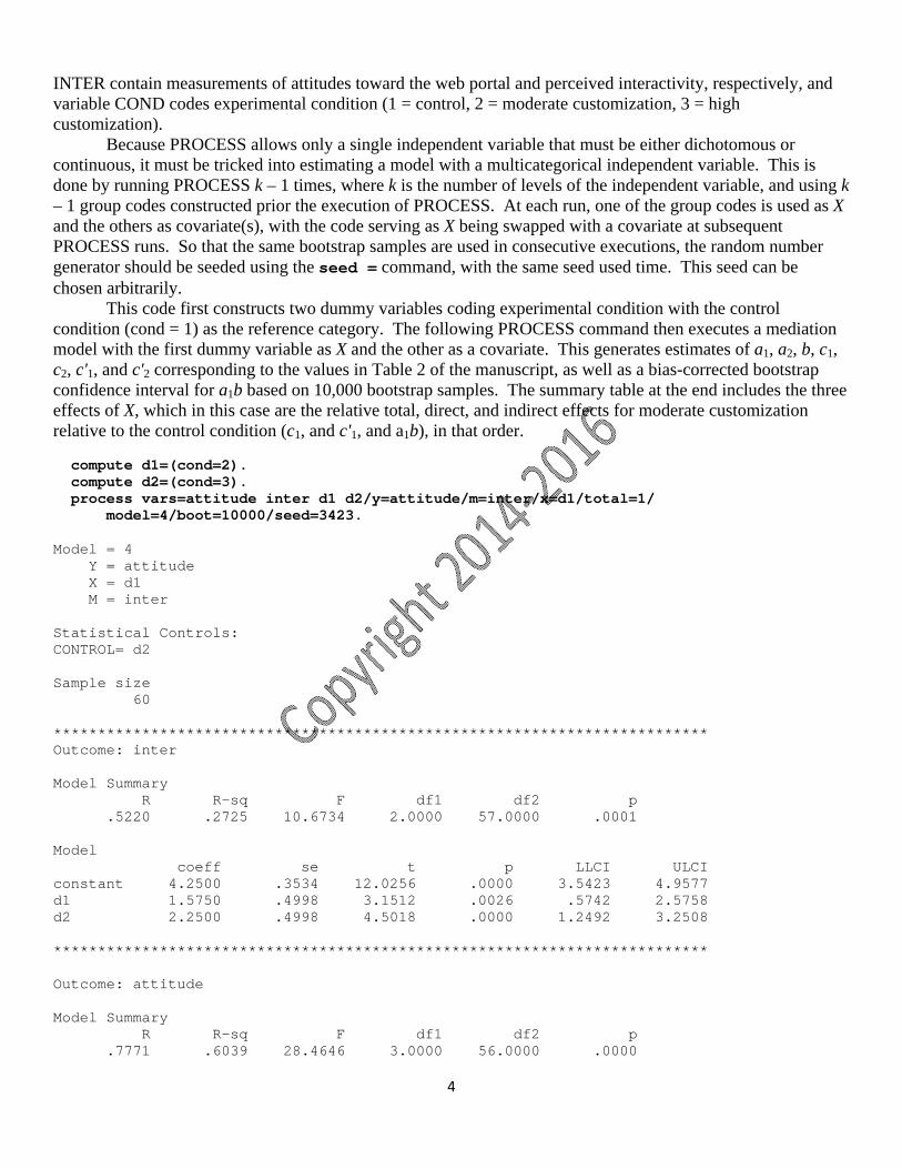
INTER contain measurements of attitudes toward the web portal and perceived interactivity, respectively, and variable COND codes experimental condition (1 = control, 2 = moderate customization, 3 = high customization).

Because PROCESS allows only a single independent variable that must be either dichotomous or continuous, it must be tricked into estimating a model with a multicategorical independent variable. This is done by running PROCESS k – 1 times, where k is the number of levels of the independent variable, and using k – 1 group codes constructed prior the execution of PROCESS. At each run, one of the group codes is used as X and the others as covariate(s), with the code serving as X being swapped with a covariate at subsequent PROCESS runs. So that the same bootstrap samples are used in consecutive executions, the random number generator should be seeded using the seed = command, with the same seed used time. This seed can be chosen arbitrarily.

This code first constructs two dummy variables coding experimental condition with the control condition (cond = 1) as the reference category. The following PROCESS command then executes a mediation model with the first dummy variable as X and the other as a covariate. This generates estimates of a1, a2, b, c1, c2, c'1, and c'2 corresponding to the values in Table 2 of the manuscript, as well as a bias-corrected bootstrap confidence interval for a1b based on 10,000 bootstrap samples. The summary table at the end includes the three effects of X, which in this case are the relative total, direct, and indirect effects for moderate customization relative to the control condition (c1, and c'1, and a1b), in that order. compute d1=(cond=2). compute d2=(cond=3). process vars=attitude inter d1 d2/y=attitude/m=inter/x=d1/total=1/ model=4/boot=10000/seed=3423. Model = 4 Y = attitude X = d1 M = inter Statistical Controls: CONTROL= d2 Sample size 60 ************************************************************************** Outcome: inter Model Summary R R-sq F df1 df2 p .5220 .2725 10.6734 2.0000 57.0000 .0001 Model coeff se t p LLCI ULCI constant 4.2500 .3534 12.0256 .0000 3.5423 4.9577 d1 1.5750 .4998 3.1512 .0026 .5742 2.5758 d2 2.2500 .4998 4.5018 .0000 1.2492 3.2508 ************************************************************************** Outcome: attitude Model Summary R R-sq F df1 df2 p .7771 .6039 28.4646 3.0000 56.0000 .0000

5

Model coeff se t p LLCI ULCI constant 2.8100 .4701 5.9772 .0000 1.8682 3.7517 inter .3588 .0937 3.8302 .0003 .1712 .5465 d1 1.1048 .3831 2.8842 .0056 .3375 1.8722 d2 2.1576 .4116 5.2423 .0000 1.3331 2.9821 ************************** TOTAL EFFECT MODEL **************************** Outcome: attitude Model Summary R R-sq F df1 df2 p .7072 .5002 28.5213 2.0000 57.0000 .0000 Model coeff se t p LLCI ULCI constant 4.3350 .2783 15.5749 .0000 3.7776 4.8924 d1 1.6700 .3936 4.2426 .0001 .8818 2.4582 d2 2.9650 .3936 7.5326 .0000 2.1768 3.7532 ***************** TOTAL, DIRECT, AND INDIRECT EFFECTS ******************** Total effect of X on Y Effect SE t p LLCI ULCI 1.6700 .3936 4.2426 .0001 .8818 2.4582 Direct effect of X on Y Effect SE t p LLCI ULCI 1.1048 .3831 2.8842 .0056 .3375 1.8722 Indirect effect of X on Y Effect Boot SE BootLLCI BootULCI inter .5652 .2724 .1643 1.2665 ******************** ANALYSIS NOTES AND WARNINGS ************************* Number of bootstrap samples for bias corrected bootstrap confidence intervals: 10000 Level of confidence for all confidence intervals in output: 95.00

Missing from the output above is the relative indirect effect for high customization relative to none (a2b) along with a bootstrap confidence interval for inference. The code below generates this relative indirect effect by switching d1 and d2 in the x= specification. Most of the output is identical to the code generated by the command above, so that output is suppressed by using the detail=0 option. Using the same random number seed as in the prior run of PROCESS produces a bootstrap confidence interval based on the same set of bootstrap samples. The effects for X in this summary table are the relative total, direct, and indirect effects for high customization relative to the control condition (c2, c'2, and a2b), in that order. process vars=attitude inter d1 d2/y=attitude/m=inter/x=d2/total=1/ model=4/boot=10000/seed=3423/detail=0. Model = 4 Y = attitude X = d2 M = inter

6

Statistical Controls: CONTROL= d1 Sample size 60 ***************** TOTAL, DIRECT, AND INDIRECT EFFECTS ******************** Total effect of X on Y Effect SE t p LLCI ULCI 2.9650 .3936 7.5326 .0000 2.1768 3.7532 Direct effect of X on Y Effect SE t p LLCI ULCI 2.1576 .4116 5.2423 .0000 1.3331 2.9821 Indirect effect of X on Y Effect Boot SE BootLLCI BootULCI inter .8074 .3273 .3217 1.6442 ******************** ANALYSIS NOTES AND WARNINGS ************************* Number of bootstrap samples for bias corrected bootstrap confidence intervals: 10000 Level of confidence for all confidence intervals in output: 95.00

The SPSS compute commands above generate indicator codes with the control group as the reference group. The commands to generate the contrast codes used in the example analysis would be if (cond=1) d1 = -0.667. if (cond=1) d2 = 0. if (cond=2) d1 = 0.333. if (cond=2) d2 = -0.5. if (cond=3) d1 = 0.333. if (cond=3) d2 = 0.5. For the sequential coding example described below, the following SPSS commands construct the sequential codes: compute d1 = (cond > 1). compute d2 = (cond > 2).

The PROCESS macro is available for SAS but requires PROC IML. The command structure is very similar to the SPSS version, but the construction of group codes requires commands that are different than those used in SPSS. The SAS code below conducts the example analysis using indicator coding of groups, assuming the data reside in a SAS data file named “web”: data web;set web;d1=(cond=2);d2=(cond=3);run; %process (data=web,vars=attitude inter d1 d2,y=attitude,m=inter,x=d1, total=1,model=4,boot=10000,seed=3423); %process (data=web,vars=attitude inter d1 d2,y=attitude,m=inter,x=d2, total=1,model=4,boot=10000,seed=3423,detail=0);

7

For the contrast codes corresponding to the example analysis in this paper, change the DATA line to read: data web;set web; if (cond=1) then do;d1=-0.667;d2=0;end; if (cond=2) then do;d1=0.333;d2=-0.5;end; if (cond=3) then do;d1=0.333;d2=0.5;end; run; For the sequential codes described in the example below, the DATA line should read data web;set web;d1=(cond>1);d2=(cond>2);run;

Estimation using MEDIATE for SPSS NOTE: The text in this section is what was provided to the journal when the article was published. Since this paper was published, a feature was added to PROCESS that allows for the specification of X as a multicategorical variable in model 4. The resulting PROCESS output looks very similar to what MEDIATE produces. MEDIATE is a freely available SPSS macro (downloadable from [web address blinded for review]) that facilitates the estimation of mediation models with multicategorical independent variables along with the ability to generate bootstrap confidence intervals for indirect effects. It is very limited in its features relative to PROCESS, but it does have one handy option that automates the construction of codes for a categorical independent variable. The code and output below corresponds to the analysis of the web portal customization study using indicator coding of customization condition. Variables named ATTITUDE and INTER contain measurements of attitudes toward the web portal and perceived interactivity, respectively, and variable COND codes experimental condition (1 = control, 2 = moderate customization, 3 = high customization). The catx=1 option specifies indicator coding and sets the control condition as the reference group. See the documentation for additional information about the MEDIATE macro and its options. mediate y=attitude/x=cond/m=inter/samples=10000/total=1/catx=1. Run MATRIX procedure: VARIABLES IN THE FULL MODEL: Y = attitude M1 = inter X = cond CODING OF CATEGORICAL X FOR ANALYSIS: cond D1 D2 1.0000 .0000 .0000 2.0000 1.0000 .0000 3.0000 .0000 1.0000 ***************************************************************************** OUTCOME VARIABLE: attitude MODEL SUMMARY (TOTAL EFFECTS MODEL) R R-sq Adj R-sq F df1 df2 p .7072 .5002 .4826 28.5213 2.0000 57.0000 .0000

8

MODEL COEFFICIENTS (TOTAL EFFECTS MODEL) Coeff. s.e. t p Constant 4.3350 .2783 15.5749 .0000 D1 1.6700 .3936 4.2426 .0001 D2 2.9650 .3936 7.5326 .0000 ***************************************************************************** OUTCOME VARIABLE: inter MODEL SUMMARY R R-sq Adj R-sq F df1 df2 p .5220 .2725 .2469 10.6734 2.0000 57.0000 .0001 MODEL COEFFICIENTS Coeff. s.e. t p Constant 4.2500 .3534 12.0256 .0000 D1 1.5750 .4998 3.1512 .0026 D2 2.2500 .4998 4.5018 .0000 ***************************************************************************** OUTCOME VARIABLE: attitude MODEL SUMMARY R R-sq adj R-sq F df1 df2 p .7771 .6039 .5827 28.4646 3.0000 56.0000 .0000 MODEL COEFFICIENTS Coeff. s.e. t p Constant 2.8100 .4701 5.9772 .0000 inter .3588 .0937 3.8302 .0003 D1 1.1048 .3831 2.8842 .0056 D2 2.1576 .4116 5.2423 .0000 TEST OF HOMOGENEITY OF REGRESSION (X*M INTERACTION) R-sq F df1 df2 p inter .0043 .2969 2.0000 54.0000 .7443 ***************************************************************************** INDIRECT EFFECT(S) THROUGH: inter Effect SE(boot) LLCI ULCI D1 .5652 .2694 .1693 1.2548 D2 .8074 .3252 .3338 1.6587 ---------- ********************* ANALYSIS NOTES AND WARNINGS ************************* NOTE: Indicator coding is used for categorical X Number of samples used for indirect effect confidence intervals: 10000 Level of confidence for confidence intervals: 95.0000

9

Bias corrected bootstrap confidence intervals for indirect effects are printed in output

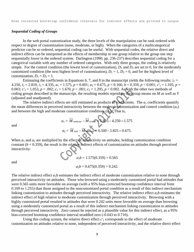
Sequential Coding of Groups In the web portal customization study, the three levels of the manipulation can be rank ordered with

respect to degree of customization (none, moderate, or high). When the categories of a multicategorical predictor can be so ordered, sequential coding can be useful. With sequential codes, the relative direct and indirect effects can be interpreted as the effects of membership in one group relative to the group one step sequentially lower in the ordered system. Darlington (1990, pp. 236-237) describes sequential coding for a categorical variable with any number of ordered categories. With only three groups, the coding is relatively simple. For the control condition (the lowest level of customization), D1 and D2 are set to 0, for the moderately customized condition (the next highest level of customization), D1 = 1, D2 = 0, and for the highest level of customization, D1 = D2 = 1.

Estimating the coefficients in Equations 6, 7, and 8 in the manuscript yields the following results: i1 = 4.250, i2 = 2.810, i3 = 4.335, a1 = 1.575, p = 0.001; a2 = 0.675, p = 0.166; b = 0.359, p < 0.001; c'1 = 1.105, p = 0.003; c'2 = 1.053, p = .002; c1 = 1.670, p < .001; c2 = 1.295, p < 0.002. As with the other two methods of coding groups described in the manuscript, the resulting models reproduce the group means on M as well as Y (adjusted and unadjusted). The relative indirect effects are still estimated as products of coefficients. The a1 coefficients quantify the mean differences in perceived interactivity between the moderate customization and control condition (a1) and between the high and moderate customization conditions (a2). That is,

a1 = 5.825 4.250 1.575moderate controlM M and

a2 = 6.500 5.825 0.675high moderateM M .

When a1 and a2 are multiplied by the effect of interactivity on attitudes, holding customization condition constant (b = 0.359), the result is the relative indirect effects of customization on attitudes through perceived interactivity:

a1b = 1.575(0.359) = 0.565 and

a2b = 0.675(0.359) = 0.242.

The relative indirect effect a1b estimates the indirect effect of moderate customization relative to none through perceived interactivity on attitudes. Those who browsed using a moderately customized portal had attitudes that were 0.565 units more favorable on average (with a 95% bias-corrected bootstrap confidence interval from 0.169 to 1.255) than those assigned to the noncustomized portal condition as a result of this indirect mechanism linking customization to attitudes through perceived interactivity. The relative indirect effect a2b estimates the indirect effect of high relative to moderate customization through perceived interactivity. Browsing with a highly customized portal resulted in attitudes that were 0.242 units more favorable on average than browsing using a moderately customized portal as a result of this indirect mechanism linking customization to attitudes through perceived interactivity. Zero cannot be rejected as a plausible value for this indirect effect, as a 95% bias-corrected bootstrap confidence interval straddled zero (-0.043 to 0.710).

Using this coding system, the relative direct effect c'1 corresponds to the effect of moderate customization on attitudes relative to none, independent of perceived interactivity, and the relative direct effect

10

c'2 is the effect of high customization relative to moderate customization. This corresponds to differences between the adjusted means:

c'1 = *

moderateY – *

controlY = 5.897 – 4.792 = 1.105

c'2 = *

highY – *

moderateY = 6.950 – 5.897 = 1.053.

As when other coding systems are used, the relative total effects can be estimated using Equation 8 in the manuscript or by adding the relative direct and indirect effects. With sequential coding, c1 estimates the mean difference in attitude between the moderately customized and control groups, and c2 estimates the mean difference in attitude between the highly customized and moderately customized groups. That is,

c1 = 6.005 4.335 1.670moderate controlY Y

c2 = 7.300 6.005 1.295high moderateY Y .

As both effects are positive, this suggests attitudes increase in favorability as customization increases. Finally, notice that as with indicator or contrast coding, the relative total effects partition cleanly into the relative direct and relative indirect effects: c1 = c'1 + a1b = 1.105 + 0.565 = 1.670 and c2 = c'2 + a2b = 1.053 + 0.242 = 1.295. Random Measurement Error

The example analyses in the manuscript and this supplement ignore the potential influence of random measurement error in X, M, or Y. In experiments, and even when X is an observed categorical variable, measurement error in X is often negligible to nonexistent unless the categories were constructed through some kind of artificial categorization of a continuum or there is some ambiguity or subjectivity in the decision as to which category a particular case in the data belongs. But M and/or Y may and often do contain some random measurement error, such as when they are sum scores from a psychological test, personality inventory, or attitude scale. If M, Y, or both is measured with error, the result is bias in the estimation of the effects of X, reduced statistical power, or both (see, e.g., Darlington, 1990, pp. 201-204; Ledgerwood & Shrout, 2012). The method described in the manuscript can easily be extended using Mplus or another SEM program using single indicator latent variables with reliability-weighted errors (see e.g., Kline, 2005) or latent variable model with a measurement model component that links the latent variable causally to its indicators. Both approaches potentially reduce at least some of the deleterious effects of random measurement error. As with any measurement model, the researcher should ascertain whether the measurement model for the latent variable(s) satisfies various criteria for claiming “good fit,” for direct and indirect effects linking latent variables that are not modeled well have little substantive meaning. For discussions of latent variable mediation analysis, see Cheung and Lau (2008), Coffman and MacCallum (2005), Lau and Cheung (2012), and MacKinnon (2008). Multiple Mediators

The approach we have illustrated for estimating relative indirect and direct effects can be extended to models with any number (m) of mediators operating in parallel. Figure S1 depicts a model with m proposed mediators and a multicategorical X with k categories. The relative total effects, ci, can be estimated if desired using Equation 8 in the manuscript, whereas the relative indirect and direct effects are pieced together from parameter estimates from m + 1 linear models, one for each of the m mediators and one for Y:

Mj = i1j + a1jD1 + a2jD2 + . . . + a(k-1)jDk-1 + eMj (S1)

Y = i2 + c'1D1 + c'2D2 + . . . + c'k-1Dk-1 + b1M1 + b2M2 + . . . + bmMm + eY (S2)

11

The same relationships among relative total, indirect, and direct effects exist in multiple-mediator models as in single-mediator models. The relative total effect for Di can be partitioned into the relative direct effect for Di plus the sum of the relative specific indirect effects for Di, ai1b1 + ai2b2 + . . . + aimbm. That is,

1

m

i i ij jjc c a b

(S3)

This last term in Equation S3 is the relative total indirect effect of Di. Each relative specific indirect effect quantifies the component of the relative total indirect effect that is carried uniquely through that mediator. Inferential tests of relative specific indirect effects can be undertaken just as described in the manuscript, and these would typically be the focus of a mediation analysis. The Mplus code above can be modified without difficulty to include multiple mediators, and the PROCESS and MEDIATE procedures for SPSS and SAS allow for multiple mediators operating in parallel in this fashion. See the documentation. Covariates and Confounds In a mediation model, the interpretation of an indirect effect as a causal one assumes that the mediator M is causally located between X and Y. That is, it is assumed that X causes M and M causes Y. When X is experimentally manipulated and sound experimental procedures are followed, a causal association between X and M and between X and Y is established by showing that the k groups differ on M and Y on average. Of course, as many others have emphasized before us (e.g., Bullock et al., 2010; Hayes, 2013; Mathieu, DeShon, & Bergh, 2008; Stone-Romero & Rosopa, 2010), this does not establish that M causes Y. It could be that Y causes M or that M and Y are spuriously associated (both are caused by some variable W) or epiphenomenally associated (M is correlated with the “true” intermediary variable W). If X is not experimentally manipulated, such threats to causal inference also exist in the interpretation of the association between X and M as well.

Spuriousness and epiphenomenality, as alternative explanations at least with respect to a given competing variable W, can be accounted for in a mediation model by including W as an additional predictor or “covariate” in the models of M and Y. For example, Equations 1, 2, and 3 in the manuscript with the inclusion of W as a covariate would be

M = i1 + aX + d1W + eM (S4)

Y = i2 + c'X + bM + d2W + eY (S5) Y = i3 + cX + d3W+ eY (S6)

The addition of covariates is simple in any OLS regression program; covariates can be added to each of the ON statements in the Mplus code above, and the PROCESS and MEDIATE macros also accept covariates.

References Bullock, J. G., Green, D. P., & Ha, S. E. (2010). Yes, but what is the mechanism? (Don’t expect an easy

answer). Journal of Personality and Social Psychology, 98, 550-558. Cheung, G. W., & Lau, R. S. (2008). Testing mediation and suppression effects of latent variables:

Bootstrapping with structural equation models. Organizational Research Methods, 11, 296-325. Coffman, D. L., & MacCallum, R. C. (2005). Using parcels to convert path models into latent variable models.

Multivariate Behavioral Research, 40, 235-259. Darlington, R. B. (1990). Regression and linear models. New York: McGraw-Hill. Hayes, A. F. (2013). An introduction to mediation, moderation, and conditional process analysis. New York:

The Guilford Press.

12

Hayes, A. F., & Preacher, K. J. (2014). Statistical mediation analysis with a multicategorical independent variable. British Journal of Mathematical and Statistical Psychology, 67, 451-470.

Kline, R. B. (2005). Principles and practices of structural equation modeling (2nd Ed.). New York: Guilford Press.

Lau, R. S., & Cheung, G. W. (2012). Estimating and comparing specific mediation effects in complex latent variable models. Organizational Research Methods, 15, 3-16.

Ledgerwood, A., & Shrout, P. E. (2011). The trade-off between accuracy and precision in latent variable models of mediation processes. Journal of Personality and Social Psychology, 101, 1174-1188.

MacKinnon, D. P. (2008). An introduction to statistical mediation analysis. New York: Routledge. Mathieu, J. E., DeShon, R. P., & Bergh, D. D. (2008). Mediational inferences in organizational research.

Organizational Research Methods, 11, 203-223. Preacher, K. J., & Hayes, A. F. (2008). Asymptotic and resampling strategies for assessing and comparing

indirect effects in multiple mediator models. Behavior Research Methods, 40, 879-891. Stone-Romero, E. F., & Rosopa, P. J. (2010). Research design options for testing mediation models and their

implications for facets of validity. Journal of Managerial Psychology, 25, 697-712.

13

Figure S1. A multiple mediation model in path diagram form corresponding to a model with an independent variable X with k categories and m mediators operating in parallel. When estimating using a structural equation modeling program, it is recommended that the covariance between mediator errors be freely estimated (see e.g., Preacher and Hayes, 2008).

Date post:	06-Dec-2021
Category:	Documents
Upload:	others
View:	2 times
Download:	0 times

Expert Tutorial Statistical mediation analysis with a ...

Documents