Universita’ degli studi di Roma “Tor Vergata”

Facolta’ di Ingegneria Elettronica

Dottorato di Ricerca in Ingegneria delle Telecomunicazioni e

Microelettronica

XX Ciclo

Channel Quality Estimation and Impairment Mitigation in 802.11Networks

Tesi di Dottorato di

Domenico Giustiniano

Docente Guida/Tutor: Prof. Giuseppe Bianchi

Coordinatore: Prof. Nicola Blefari Melazzi

I hereby declare that this submission is my own work and that, to the best of my knowledge and

belief, it contains no material previously published or written by another person nor material which

to a substantial extent has been accepted for the award of any other degree or diploma of the

university or other institute of higher learning.

Domenico Giustiniano

CONTENTS

Contents i

Acknowledgments v

Abstract vi

1 Introduction 1

1.1 Background material . . . . . . . . . . . . . . . . . . . . . . . . . . . . . . . . . . . . . 1

1.1.1 Network Operation Modes . . . . . . . . . . . . . . . . . . . . . . . . . . . . . . 3

1.2 Challenges and Contributions . . . . . . . . . . . . . . . . . . . . . . . . . . . . . . . . 4

1.2.1 Physical Channel Impairments . . . . . . . . . . . . . . . . . . . . . . . . . . . 4

1.2.2 MAC Channel Impairments . . . . . . . . . . . . . . . . . . . . . . . . . . . . . 7

1.2.3 MAC/PHY Channel Impairments . . . . . . . . . . . . . . . . . . . . . . . . . 7

1.2.4 802.11 Quality Status . . . . . . . . . . . . . . . . . . . . . . . . . . . . . . . . 9

1.3 Publications . . . . . . . . . . . . . . . . . . . . . . . . . . . . . . . . . . . . . . . . . . 10

2 Switching Diversity: An explanation for unexpected 802.11 Outdoor Link-level

Measurement Results 13

2.1 Introduction . . . . . . . . . . . . . . . . . . . . . . . . . . . . . . . . . . . . . . . . . . 13

2.2 Reference Material . . . . . . . . . . . . . . . . . . . . . . . . . . . . . . . . . . . . . . 16

2.2.1 PHY Channel Quality Measurements Methods . . . . . . . . . . . . . . . . . . 16

2.2.2 Diversity Mechanisms in 802.11 Cards . . . . . . . . . . . . . . . . . . . . . . . 17

2.3 Measurement Scenario . . . . . . . . . . . . . . . . . . . . . . . . . . . . . . . . . . . . 20

2.4 Experimental Results . . . . . . . . . . . . . . . . . . . . . . . . . . . . . . . . . . . . . 22

2.4.1 Transmit Diversity on Broadcast Data Frames . . . . . . . . . . . . . . . . . . 23

2.4.2 Transmit Diversity on Unicast Data Frames . . . . . . . . . . . . . . . . . . . . 26

2.5 Validation in Indoor Controlled Links and Extension to Intel Cards . . . . . . . . . . . 27

i

2.5.1 Methodology . . . . . . . . . . . . . . . . . . . . . . . . . . . . . . . . . . . . . 28

2.5.2 Validation of Transmit Diversity on Atheros Cards . . . . . . . . . . . . . . . . 28

2.5.3 Tests on Intel cards . . . . . . . . . . . . . . . . . . . . . . . . . . . . . . . . . 31

2.6 Conclusions . . . . . . . . . . . . . . . . . . . . . . . . . . . . . . . . . . . . . . . . . . 32

3 Interference Mitigation and Multipath Tolerance in 802.11b/g Outdoor Wireless

Links 35

3.1 Introduction . . . . . . . . . . . . . . . . . . . . . . . . . . . . . . . . . . . . . . . . . . 35

3.2 Undisclosing the Interference Mitigation Procedure . . . . . . . . . . . . . . . . . . . . 37

3.3 Measurement Scenario and Link/traffic Settings . . . . . . . . . . . . . . . . . . . . . . 38

3.4 Experimental Results . . . . . . . . . . . . . . . . . . . . . . . . . . . . . . . . . . . . . 38

3.4.1 Understanding the Impact of Interference Mitigation . . . . . . . . . . . . . . . 38

3.4.2 Received Frames and Causes of Errors . . . . . . . . . . . . . . . . . . . . . . . 40

3.5 Interpretation of Packet Losses in 802.11g . . . . . . . . . . . . . . . . . . . . . . . . . 42

3.5.1 802.11b Multipath Tolerance . . . . . . . . . . . . . . . . . . . . . . . . . . . . 42

3.5.2 802.11g Multipath Tolerance . . . . . . . . . . . . . . . . . . . . . . . . . . . . 43

3.6 Conclusions . . . . . . . . . . . . . . . . . . . . . . . . . . . . . . . . . . . . . . . . . . 44

4 802.11 Link-distance Estimation 47

4.1 Introduction . . . . . . . . . . . . . . . . . . . . . . . . . . . . . . . . . . . . . . . . . . 47

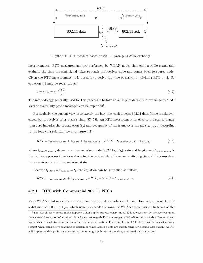
4.2 Background on RTT Link-distance Estimates . . . . . . . . . . . . . . . . . . . . . . . 48

4.2.1 RTT with Commercial 802.11 NICs . . . . . . . . . . . . . . . . . . . . . . . . 49

4.2.2 RTT with Enhanced 802.11 Hardware . . . . . . . . . . . . . . . . . . . . . . . 50

4.3 Our Methodology . . . . . . . . . . . . . . . . . . . . . . . . . . . . . . . . . . . . . . . 50

4.4 Experimental Results . . . . . . . . . . . . . . . . . . . . . . . . . . . . . . . . . . . . . 51

4.5 Conclusions . . . . . . . . . . . . . . . . . . . . . . . . . . . . . . . . . . . . . . . . . . 54

5 MAC Channel Quality Estimator 55

5.1 Introduction . . . . . . . . . . . . . . . . . . . . . . . . . . . . . . . . . . . . . . . . . . 55

5.2 Related Work . . . . . . . . . . . . . . . . . . . . . . . . . . . . . . . . . . . . . . . . . 57

5.3 Link Impairments . . . . . . . . . . . . . . . . . . . . . . . . . . . . . . . . . . . . . . . 57

5.4 Estimating Link Quality . . . . . . . . . . . . . . . . . . . . . . . . . . . . . . . . . . . 59

5.4.1 Estimating Noise Errors . . . . . . . . . . . . . . . . . . . . . . . . . . . . . . . 60

5.4.2 Estimating Hidden Node Interference . . . . . . . . . . . . . . . . . . . . . . . 61

5.4.3 Estimating Collision Rate . . . . . . . . . . . . . . . . . . . . . . . . . . . . . . 61

5.5 Impairments that do not lead to Frame Loss . . . . . . . . . . . . . . . . . . . . . . . . 62

5.5.1 MAC Slots . . . . . . . . . . . . . . . . . . . . . . . . . . . . . . . . . . . . . . 62

5.5.2 Capture and Exposed Nodes . . . . . . . . . . . . . . . . . . . . . . . . . . . . 63

5.6 Implementation on Commodity Hardware and Testbed Setup . . . . . . . . . . . . . . 65

ii

5.6.1 Implementation . . . . . . . . . . . . . . . . . . . . . . . . . . . . . . . . . . . . 65

5.6.2 Testbed Setup . . . . . . . . . . . . . . . . . . . . . . . . . . . . . . . . . . . . 65

5.6.3 Cross-Validation of Frame Loss Impairments . . . . . . . . . . . . . . . . . . . 66

5.7 Experimental Assessment . . . . . . . . . . . . . . . . . . . . . . . . . . . . . . . . . . 69

5.7.1 Collisions only, no Noise, no Hidden Nodes . . . . . . . . . . . . . . . . . . . . 69

5.7.2 Channel Noise only, no Collisions, no Hidden Nodes . . . . . . . . . . . . . . . 70

5.7.3 Hidden Nodes only, no Collisions, no Noise . . . . . . . . . . . . . . . . . . . . 71

5.7.4 Collisions and Hidden Nodes, no Noise . . . . . . . . . . . . . . . . . . . . . . . 73

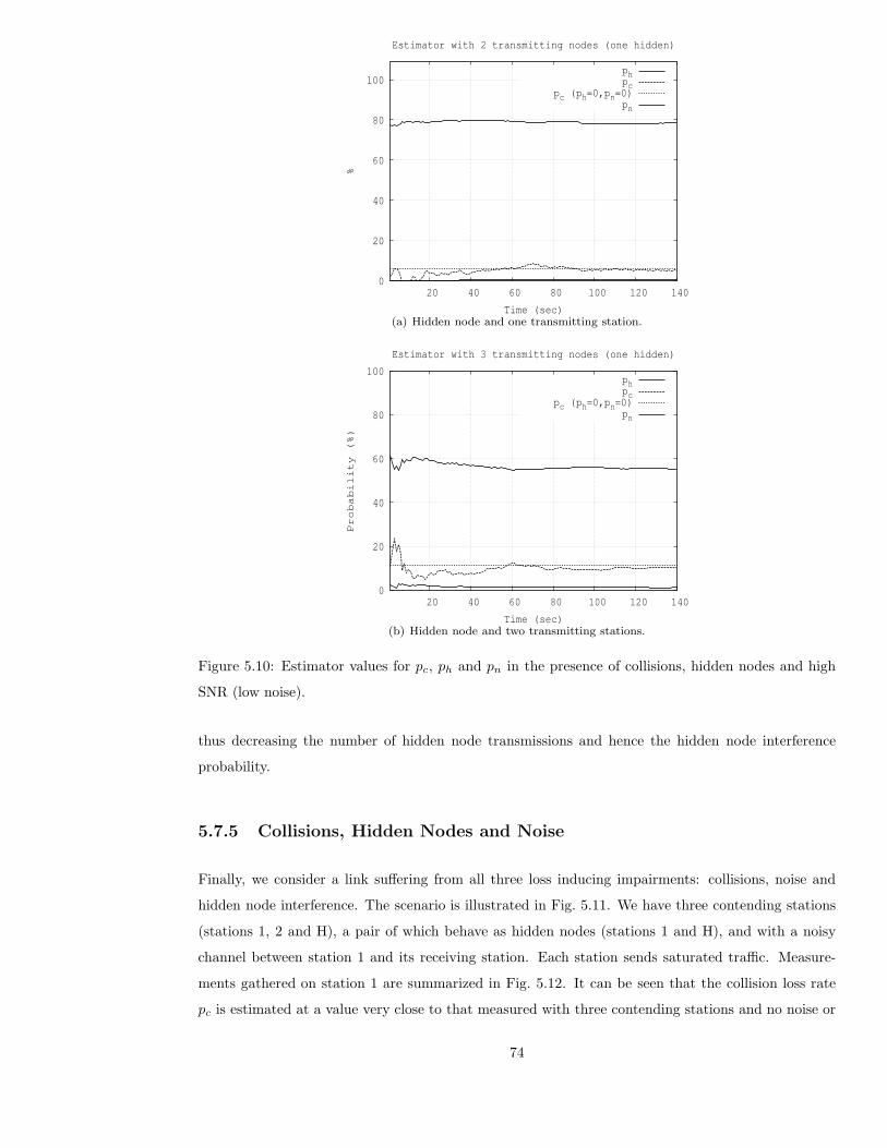
5.7.5 Collisions, Hidden Nodes and Noise . . . . . . . . . . . . . . . . . . . . . . . . 74

5.8 Estimating Exposed Node and Capture Effects . . . . . . . . . . . . . . . . . . . . . . 75

5.8.1 Exposed Nodes . . . . . . . . . . . . . . . . . . . . . . . . . . . . . . . . . . . . 75

5.8.2 Physical Layer Capture . . . . . . . . . . . . . . . . . . . . . . . . . . . . . . . 79

5.9 Conclusions . . . . . . . . . . . . . . . . . . . . . . . . . . . . . . . . . . . . . . . . . . 80

5.10 Appendix: Remarks on Hidden Nodes . . . . . . . . . . . . . . . . . . . . . . . . . . . 83

5.10.1 Performance of RTS/CTS with Hidden Nodes . . . . . . . . . . . . . . . . . . . 83

5.10.2 CRC Errors with Hidden Nodes . . . . . . . . . . . . . . . . . . . . . . . . . . . 85

6 Hidden ACK Interference in 802.11 Multi-Cell Networks and its Mitigation 87

6.1 Introduction . . . . . . . . . . . . . . . . . . . . . . . . . . . . . . . . . . . . . . . . . . 87

6.2 Hidden ACK Phenomenon . . . . . . . . . . . . . . . . . . . . . . . . . . . . . . . . . . 89

6.3 Successive Interference Cancellation for Hidden ACKs . . . . . . . . . . . . . . . . . . 91

6.4 System Model of the Simulator . . . . . . . . . . . . . . . . . . . . . . . . . . . . . . . 93

6.4.1 Transmitter: IEEE 802.11g . . . . . . . . . . . . . . . . . . . . . . . . . . . . . 93

6.4.2 Channel . . . . . . . . . . . . . . . . . . . . . . . . . . . . . . . . . . . . . . . . 93

6.4.3 Receiver: SIC decoder . . . . . . . . . . . . . . . . . . . . . . . . . . . . . . . . 94

6.5 Performance Evaluation and Topological Interpretation of the Results . . . . . . . . . 94

6.5.1 Topological Interpretation . . . . . . . . . . . . . . . . . . . . . . . . . . . . . . 96

6.6 Conclusions . . . . . . . . . . . . . . . . . . . . . . . . . . . . . . . . . . . . . . . . . . 97

7 Conclusions and Suggestions for Further Works 99

Appendix 101

7.1 Link-distance Estimation based on SNR Measurements . . . . . . . . . . . . . . . . . . 101

7.1.1 Link-distance Estimate based on SNR . . . . . . . . . . . . . . . . . . . . . . . 101

7.1.2 Experimental Assessment . . . . . . . . . . . . . . . . . . . . . . . . . . . . . . 101

7.2 Link Analysis Tool for Outdoor Testbeds: the Statistics Gathering Approach . . . . . 106

List of figures 110

List of tables 113

iii

Bibliography 115

iv

ACKNOWLEDGMENTS

First of all, I would like to thank my parents for their support in all these years. My father has always

dreamed that I take the chance in my life that he could not have when he was young. My mother

has supported me with patience and kindness. I could not have any good idea in my work without

her lovely food. But any word is not enough to explain how their have been important for each day

of my student life.

Then, I really need to thank my brother, Alessandro, and sisters, Anna and Angela. A life could

be boring without such a wonderful combination of skills and capabilities. I am proud to be their

brother.

I gratefully thank the Netgroup Lab in Rome, the Telecommunication Lab in Maynooth and

my friends/colleagues: Alessandro Ordine, Aysun Celik, Chiara Santoro, Dimitri Ognibene, Fab-

rizio Formisano, Fernanda Viola, Vincenzo Mancuso, Filippo Munisteri, Luca Scalia, Mauro Barresi,

Roberto Spiga, Vincenzo Dina. A sincere thanks is for Ilenia Tinnirello, for her help and friendship

in these years.

A thank is also for Nicola Blefari Melazzi, David Malone, and Doug Leith for their precious advices.

And finally I express a special acknowledgment and deep gratitude to my supervisor and friend

Giuseppe Bianchi, that teached me all the methods and secrets in our work, but also the enthusiasm

for the research. Thanks Giuseppe!

v

vi

ABSTRACT

Wireless communication has been boosted by the adoption of 802.11 as standard de facto for WLAN

transmission. Born as a niche technology for providing wireless connectivity in small office/enterprise

environments, 802.11 has in fact become a common and cheap access solution to the Internet, thanks to

the large availability of wireless gateways (home modems, public hot-spots, community networks, and

so on). Nowdays, the trend towards increasingly dense 802.11 wireless deployments is creating a real

need for effective approaches for channel allocation/hopping, power control, etc. for interference miti-

gation while new applications such mesh networks in outdoor contexts and media distribution within

the home are creating new quality of service demands that require more sophisticated approaches to

radio resource allocation.

The new framework of WLAN deployments require a complete understanding of channel quality

at PHY and MAC layer. Goal of this thesis is to assess the MAC/PHY channel quality and miti-

gate the different channel impairments in 802.11 networks, both in dense/controlled indoor scenarios

and emerging outdoor contexts. More specifically, chapter 1 deals with the necessary background

material and gives insight into the different channel impairments/quality it can be encountered in

WLAN networks. Then the thesis pursues a down/top approach: chapter 2, 3 and 4 aim at affording

impairments/quality at PHY level, while chapter 5 and 6 analyse channel impairments/quality from

a MAC level perspective.

An important contribution of this thesis is to undisclose that some PHY layer parameters, such

as the transmission power, the antenna selection, and interference mitigation scheme, have a deep

impact on network performance. Since the criteria for selecting these parameters is left to the vendor

specific implementations, the performance spread of most experimental results about 802.11 WLAN

could be affected by vendor proprietary schemes. Particularly, in chapter 2 we find that switching

transmit diversity mechanisms implemented in off-the-shelf devices with two antenna connectors can

dramatically affect both performance and link quality probing mechanisms in outdoor medium-range

WLAN deployments, whenever one antenna deterministically works worse than the other one. A

vii

second physical algorithm with side-effects is shown in chapter 3. Particulary the chapter shows that

interference mitigation algorithms may play havoc with the link-level testbeds, since they may erro-

neously lower the sensitivity threshold, and thus not detect the 802.11 transmit sources. Finally, once

disabled the interference mitigation algorithm — as well as any switching diversity scheme described

in the previous chapter — link-level experimental assessment concludes that, unlike 802.11b, which

appears a robust technology in most of the operational conditions, 802.11g may lead to inefficiencies

when employed in an outdoor scenario, due to the lower multi-path tolerance of 802.11g. Since multi-

path is hard to predict, a novel mechanism to improve the link-distance estimation accuracy — based

on CPU clock information — is outlined in chapter 4. The proposed methodology can not only be

applied in localization context, but also for estimating the multi-path profile.

The second part of the thesis moves the perspective to the MAC point of view and its impairments.

Particularly, chapter 5 provides the design of a MAC channel quality estimator to distinguish the

different types of MAC impairments and gives separate quantitative measures of the severity of each

one. Since the estimator takes advantage of the native characteristics of the 802.11 protocol, the

approach is suited to implementation on commodity hardware and makes available new measures

that can be of direct use for rate adaptation, channel allocation, etc. Then, chapter 6 introduces a

previous unknown phenomenon, the Hidden ACK, that may cause frame losses into multiple WLAN

networks when a node replies with an ACK frame. Again, a solution is provided without requiring

any modification to the 802.11 protocol.

Whenever possible, the quantitative analysis has been led through experimental assessments with

implementation on commodity hardware. This was the adopted methodology in chapter 2, 3, 4 and 5.

Particularly, this has required an accurate investigation of two brands of WLAN cards, particularly

the Atheros and Intel cards, and their driver/firmware, respectively MADWiFi and IPW2200, which

are currently the most adopted, respectively, by researchers and layman users.

viii

CHAPTER 1

INTRODUCTION

1.1 Background material

Today the most used technology for the wireless Internet is undoubtedly represented by IEEE 802.11

WLANs [1, 2, 3, 4, 5, 6]. Born as a niche technology for providing wireless connectivity in small

office/enterprise environments, 802.11 has in fact become a common and cheap access solution to

the Internet, thanks to the large availability of wireless gateways (home modems, public hot-spots,

community networks, and so on).

In 802.11 WLANs, the basic mechanism controlling medium access is the Distributed Coordination

Function (DCF). This is a random access scheme, based on Carrier Sense Multiple Access with Colli-

sion Avoidance (CSMA/CA). In the DCF Basic Access mode, a station with a new packet to transmit

selects a random backoff counter in the range [0,CW-1] where CW is the Contention Window. Time

is slotted and if the channel is sensed idle the station first waits for a Distributed InterFrame Space

(DIFS), then decrements the backoff counter each PHY time slot. If the channel is detected busy, the

countdown is halted and only resumed after the channel is detected idle again for a DIFS. Channel

idle/busy status is sensed via:

• CCA (Clear Channel Assessment) at physical level which is based on a carrier sense threshold

for energy/packet detection, e.g. −80dBm. The CCA module uses the Received Signal Strength

Indicator (RSSI) returned by most radio systems and expressed in absolute signal power. CCA

is expected to be updated every physical slot time. It aims to detect transmissions within the

interference range.

• NAV (Network Allocation Vector) timer at MAC level which is encapsulated in the MAC header

of each 802.11 frame and is used to accurately predict the end of a received frame on air. It

1

SIFS

BackoffDefer Access

TX Frame

Time SlotPIFS

DIFS

Busy mediumDIFS

Figure 1.1: DCF protocol summary.

is naturally updated once per packet and can only gather information from stations within the

decoding range. This method is also called virtual carrier sense.

The channel is detected as idle if the CCA detects the channel as idle and the NAV is zero. Otherwise,

the channel is detected as busy. A station transmits when the backoff counter reaches zero. The

countdown process is illustrated schematically in figure 1.1. The 802.11 handshake imposes a half-

duplex process whereby an acknowledgment (ACK) is always sent by the receiver upon the successful

receipt of a unicast frame. The ACK is sent after a period of time called the Short InterFrame Space

(SIFS). As the SIFS is shorter than a DIFS, no other station is able to detect the channel idle for a

DIFS until the end of the ACK transmission. If the transmitting station does not receive the ACK

within a specified ACK Timeout, or it detects the transmission of a different packet on the channel,

it reschedules the packet transmission according to the given backoff rules. CW is doubled with

successive referrals until a maximum value (labeled as CWmax) and is reset to the minimum value

(labeled as CWmin) after an ACKed transmission or once the maximum number of retransmission

attempts is reached.

In addition to the foregoing Basic Access mode, an optional four way handshaking technique, known

as Request-To-Send/Clear-To-Send (RTS/CTS) mode is available. Before transmitting a packet, a

station operating in RTS/CTS mode reserves the channel by sending a special Request-To-Send short

frame. The destination station acknowledges the receipt of an RTS by sending back a Clear-To-Send

frame, after which normal packet transmission and ACK response occurs. The RTS/CTS effectiveness

is largely debated. Particularly, its overhead is particularly critical [7, 8], especially when link rates

are scaled up to the 54 Mbps 802.11a/g speeds.

The DCF allows the fragmentation of packets into smaller units. Each fragment is sent as an

ordinary 802.11 frame, which the sender expects to be ACKed. However, the fragments may be sent

as a burst. That is, the first fragment contends for medium access as usual. When the first fragment is

successfully sent, subsequent fragments are sent after a SIFS, so no collisions are possible. In addition,

the medium is reserved using virtual carrier sense for the next fragment both at the sender (by setting

the 802.11 NAV field in the data fragment) and at the receiver (by updating the NAV in the ACK).

This is illustrated schematically in figure 1.2. Burst transmission is halted after the last fragment has

2

Frame BodyHDR

Fragment 0 Fragment 1

Frame BodyCRC CRCHDR

Original Frame

Figure 1.2: Fragmentation of a 802.11 Frame.

been sent or when loss is detected. Fragmentation is intended as a way to transmit longer packets

when the channel is likely to corrupt them if sent as-is.

The standard also defines an optional Point Coordination Function (PCF) [1] which is a centralized

MAC protocol able to support collision free and time bounded services. With PCF, a point coordinator

within the access point controls which stations can transmit during any give period of time. Within

a time period called the contention free period, the point coordinator will step through all stations

operating in PCF mode and poll them one at a time. For example, the point coordinator may first

poll station A, and during a specific period of time station A can transmit data frames (and no other

station can send anything). The point coordinator will then poll the next station and continue down

the polling list, while letting each station to have a chance to send data.

1.1.1 Network Operation Modes

There exist three main 802.11 network types that have been defined in the IEEE 802.11 specifications

[1, 6], structure, ad-hoc and mesh mode [9, 10], here outlined:

• infrastructure mode: in this mode, 802.11 devices called APs (Access Points) are used for all

kind of communication, including communications between 802.11 clients or stations. If a 802.11

client in an infrastructure 802.11 network needs to communicate with another 802.11 client, the

communication must take two hops. First, the originating 802.11 client transfers the frame to

the AP. Second, the AP transfers the frame to the destination client. With all communica-

tions relayed through an AP, the Basic Service Set (BSS) is defined by the set of points where

transmissions from the AP can be sent/received. So the network architecture associated with

infrastructured mode can be regarded as a type of “cell” architecture where each cell is the BSS

and each BSS is controlled by an AP.

• ad-hoc mode: stations in ad-hoc mode communicate directly with each other without any AP and

within direct communication range. The smallest possible 802.11 network is an ad-hoc network

with two stations. Typically, ad-hoc networks are composed of a small number of stations set

up for a specific purpose and for a short period of time.

3

• mesh mode: mesh nodes are fixed APs interconnected through wireless links based on the 802.11

technology themselves. Mesh nodes in the network may act as APs (Mesh AP) with respect

to the client stations in their respective BSS, as well as traffic relays with respect to other

neighboring mesh nodes via 802.11 wireless links, in order to provide wider wireless coverage.

It is also possible that some mesh nodes in the network play only the role of wireless traffic

relays for other mesh nodes, without serving any client station (Mesh Point). WLAN Mesh

networks are deployed in both the commercial world by specific vendors (e.g. Tropos Network,

Firetide, Nortel, BelAir, etc), community networks ([11, 12, 13]), and academy/research trials

(e.g. the MIT RoofNet [14], etc), and is boosting the adoption of WLAN communication in

outdoor environments.

1.2 Challenges and Contributions

Wireless channel, unlike its wire-line counterpart, has several characteristics that need to be taken

into account when designing wireless networks. Object of this section is to understand and disantagle

the causes of channel impairments, both at MAC and PHY level, into the 802.11 context. We have

identified a set of causes, summarized in table 1.1. From the user-perspective, the overall effect on

these impairments is a low throughput, a high packet delivery delay/loss, a channel access unfairness,

a low spatial reuse or any mutual correlation of them. We undertake the goal to separately analyze

each impairment and link them to the contributions of this thesis, starting from the 802.11 PHY level.

MAC layer Collisions

MAC/PHY cross-layer Hidden nodes

Exposed nodes

Capture effect

PHY layer Thermal noise/RF Interference

Multipath

Fading/Shadowing

Table 1.1: 802.11 impairments at MAC and PHY level.

1.2.1 Physical Channel Impairments

Physical transmission reliability depends on the employed modulation/coding scheme, transmission

power, antenna gain, interference immunity parameters, which should be selected according to the

perceived channel conditions, as a trade-off between transmission rate and energy consumption.

In the following we point out the different causes of frame loss at PHY level. From a MAC level

point of view, they can be simply referred as channel noise errors, since they are caused by a signal

4

to noise plus interference ratio (SNIR) under the receiver sensitivity of the wireless link.

Fading/Shadowing: Transmit Diversity Side-Effects

In order to increase the frame transmission reliability, it is possible to introduce some forms of redun-

dancy in terms of multiple observations of the transmitted signals, through multiple antenna systems

(Multiple-Input/Multiple-Output (MIMO)). Even if the interest for MIMO systems has recently ex-

ploded for future high-rate WLAN [15, 16], these solutions require more extensive signal processing,

according to the coding/diversity scheme employed, which in turns leads to an increased power dis-

sipation. Nevertheless, most of the available commercial 802.11 cards are already equipped with two

antennas. These two antennas represent a simple form of MIMO, devised to combat the fading effects

instead of enabling parallel data streams.

The antenna diversity schemes, i.e. the algorithms for selecting/combining one or two antenna

signals both at the receiver and at the transmitter side, have received much less attention than

link adaptation in experimental works about 802.11 card characterization. However, since antenna

selection is left to vendors implementations, and since diversity mechanisms are enabled by default,

their practical implementation may have some side-effect on link performance in challenging scenarios

like the outdoor WLAN network.

In chapter 2, we will show that undisclosed antenna diversity schemes, employed by most widely

used cards (namely, the Atheros and Intel based cards) can have dramatic side-effects on link perfor-

mance, although these mechanisms were devised for improving the transmission robustness to fading.

We will argue that switching diversity mechanisms have a remarkable impact on WLAN performance,

and should be carefully considered by the research community to distinguish between card-dependent

phenomena and radio propagation or protocol effects.

RF Interference and thermal Noise: Interference Mitigation Side-effects

By their nature, wireless transmissions are vulnerable to radio frequency (RF) interference from various

sources. This weakness is a growing problem for technologies that operate in the ISM frequency bands,

as these bands are becoming more crowded over time. 802.11b/g networks which use the 2.4 GHz

ISM band now compete with a wide range of wireless devices that includes 2.4 GHz cordless phones,

Bluetooth headsets, Zigbee (IEEE 802.15.5) embedded devices, 2.4 GHz RFIF tags. To promote co-

existence, devices that use the ISM band must meet a number of FCC and ITU regulations that limit

transmission power and force nodes to spread their signals. Furthermore, 802.11 uses carrier sense to

detect and defer to 802.11 and other transmitters, lower transmission rates that accommodates lower

signal-to-interference-plus-noise ratios, PHY layer coding for error correction.

These regulations only partially resolve the problem. Particularly we argue that:

5

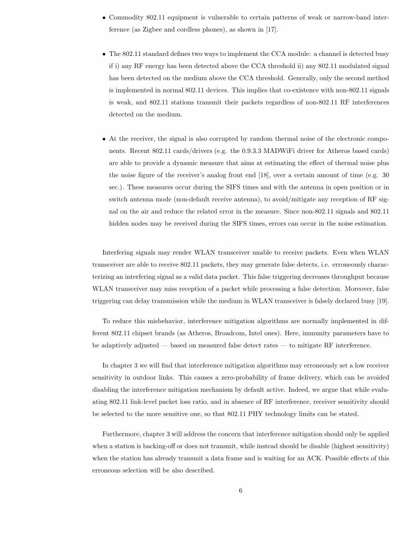
• Commodity 802.11 equipment is vulnerable to certain patterns of weak or narrow-band inter-

ference (as Zigbee and cordless phones), as shown in [17].

• The 802.11 standard defines two ways to implement the CCA module: a channel is detected busy

if i) any RF energy has been detected above the CCA threshold ii) any 802.11 modulated signal

has been detected on the medium above the CCA threshold. Generally, only the second method

is implemented in normal 802.11 devices. This implies that co-existence with non-802.11 signals

is weak, and 802.11 stations transmit their packets regardless of non-802.11 RF interferences

detected on the medium.

• At the receiver, the signal is also corrupted by random thermal noise of the electronic compo-

nents. Recent 802.11 cards/drivers (e.g. the 0.9.3.3 MADWiFi driver for Atheros based cards)

are able to provide a dynamic measure that aims at estimating the effect of thermal noise plus

the noise figure of the receiver’s analog front end [18], over a certain amount of time (e.g. 30

sec.). These measures occur during the SIFS times and with the antenna in open position or in

switch antenna mode (non-default receive antenna), to avoid/mitigate any reception of RF sig-

nal on the air and reduce the related error in the measure. Since non-802.11 signals and 802.11

hidden nodes may be received during the SIFS times, errors can occur in the noise estimation.

Interfering signals may render WLAN transceiver unable to receive packets. Even when WLAN

transceiver are able to receive 802.11 packets, they may generate false detects, i.e. erroneously charac-

terizing an interfering signal as a valid data packet. This false triggering decreases throughput because

WLAN transceiver may miss reception of a packet while processing a false detection. Moreover, false

triggering can delay transmission while the medium in WLAN transceiver is falsely declared busy [19].

To reduce this misbehavior, interference mitigation algorithms are normally implemented in dif-

ferent 802.11 chipset brands (as Atheros, Broadcom, Intel ones). Here, immunity parameters have to

be adaptively adjusted — based on measured false detect rates — to mitigate RF interference.

In chapter 3 we will find that interference mitigation algorithms may erroneously set a low receiver

sensitivity in outdoor links. This causes a zero-probability of frame delivery, which can be avoided

disabling the interference mitigation mechanism by default active. Indeed, we argue that while evalu-

ating 802.11 link-level packet loss ratio, and in absence of RF interference, receiver sensitivity should

be selected to the more sensitive one, so that 802.11 PHY technology limits can be stated.

Furthermore, chapter 3 will address the concern that interference mitigation should only be applied

when a station is backing-off or does not transmit, while instead should be disable (highest sensitivity)

when the station has already transmit a data frame and is waiting for an ACK. Possible effects of this

erroneous selection will be also described.

6

Multipath tolerance of 802.11 PHY technologies

Transmission is usually described by: i) Line-of-sight (LOS): there is a direct path between the trans-

mitter (TX) and the receiver (RX) ii) non-line-of-sight (Non-LOS): the signal arrives at the receiver

using three mechanisms of radio propagation: reflection, diffraction (when the surface encountered

has sharp edge, there is bending of the wave) and scattering (when the wave encounters object smaller

than the wavelength). If the signal is emanated from a omni-directional antenna, the energy spreads

out in all direction. In each path there are obstacle and reflectors and, moreover, the scatters close

to the terminal behave as virtual antennas. So the transmitted signals arrive at the receiver from

various directions over a multiplicity of paths. There are an unpredictable set of reflections, each with

its degree of attenuation and delay, called multipath.

The outdoor propagation environment can be significantly more disruptive than indoors. Outdoors

scatters have large spatial separation. This causes strong reflective and/or diffractive multipath effects.

The resulting RMS delay spread typically is significantly larger than indoor, where the spatial range

of scatterers is much smaller.

Our contribution is the link-level assessment of 802.11b/g technology in outdoor environments.

Since the reliability of this analysis strongly depends on correct network deployment, the analysis led

in chapter 3 needs that diversity and interference mitigation schemes were controlled and disabled.

The main result of our experimental investigation is that, unlike 802.11b, which appears a robust

technology in most of the operational conditions, 802.11g may lead to severe inefficiencies when em-

ployed in outdoor scenarios. We attribute this result to low multipath tolerance of standard 802.11g.

1.2.2 MAC Channel Impairments

From the MAC point of view, the protocol is impaired by collisions. Collisions are part of the

correct operation of CSMA/CA. A collision occurs whenever two or more stations have simultaneously

decremented their backoff counter to 0 and then transmit. The level of collision induced packet losses

is strongly load dependent. For example, 802.11b with four saturated nodes has a collision probability

of around 14% while with 20 saturated nodes the collision probability is around 40% (numbers from

the model in [20]).

Since frame losses caused by channel noise may not require that contention window is doubled

once an error occurs, a quantitative assessment of probability of collision (as discussed in chapter 5)

may allow for optimizing the contention window selection for each MAC retransmission.

1.2.3 MAC/PHY Channel Impairments

Hidden nodes, exposed nodes, capture effect depend on cross-layer interaction between the MAC

CSMA/CA protocol and PHY level parameters, namely the CCA carrier sense threshold and the

7

transmit power selected.

Hidden nodes

Frame corruption due to concurrent transmissions other than collisions are referred to as hidden node

interference and are caused by a too low sensitive CCA carrier sense value. A particular scenario,

object of chapter 6, is the hidden ACK phenomenon. Multiple parallel communications occurring

between transmit/receive node pairs separated by a sufficient distance may be suddenly impaired by

the asynchronous change of direction in the transmission occurring when a node replies with an ACK

frame. This phenomenon will be referred to as Hidden ACK Phenomenon, and we show that it can

be mitigated though a PHY layer approach based on advanced signal processing of the 802.11 signals.

Exposed nodes

Not all link impairments lead to frame loss. One such important issue is that the carrier sense

mechanism used in 802.11 to sense channel busy conditions may incorrectly classify the conditions

and operate with a too high sensitive CCA carrier sense value. Such errors lead to an unnecessary

pause in the backoff countdown and so to a reduction in achievable throughput when in fact a successful

transmission could have been made.

The exposed node effect is partially caused by false detection of non-802.11 interfering signals

as valid 802.11 data packets and partially by 802.11 stations of co-channel networks. While the first

typology of error should be mitigated as outlined in section 1.2.1, immunity to the second one requires

instead a quantitative assessment of the probability of exposed node (see chapter 5).

Capture effect

A second impairment which does not cause losses is the so-called physical layer capture (PLC), that

it the successful reception of a frame when a collision occurs. This can occur, for example, when the

colliding transmissions have different received signal power — the receiver may then be able to decode

the higher power frame. For example [21] shows that for 802.11b PLC can occur when a frame with

higher received power arrives within the physical layer preamble of a lower power frame. Differences

in received power can easily occur due to differences in the physical location of the transmitters (one

station may be closer to the receiver than others), differences in antenna gain etc. The physical layer

capture effect can lead to severe imbalance of the network resource and hence in the thoughputs

achieved by contending stations (and so to unfairness). The estimator presented in chapter 5 allows

for restoring fairness between contending stations.

8

HeaderPreamblePLCP PLCP PSDU

PHY errors

CRC errors

MACHeader MSDU CRC

Figure 1.3: Error causes at the receiver for an 802.11 frame.

1.2.4 802.11 Quality Status

Physical Error Status

Independently of the cause of frame loss, the lack of transmission reliability is simply mapped into

some frames drop. Figure 1.3 depicts the format of the transmitted Physical Protocol Data Unit

(PPDU), which is common to each 802.11a/b/g physical standard. The PPDU frame consists of a

PLCP (Physical Layer Convergence Procedure) preamble, a PLCP header and a Physical Service

Data Unit (PSDU). Each PSDU consists of the MAC header, the frame body (MSDU) and of a 32 bit

Cyclic Redundancy Check (CRC). Extra bits (Tail/Pad bits), not reported in the figure, are appended

after the CRC when OFDM is employed as modulation scheme (802.11a/g).

The PLCP preamble is carefully designed to enable synchronization. IEEE 802.11g typically uses

the ERP-OFDM mode for the PLCP format1. With the ERP-OFDM preamble, it takes just 16 µs to

train the receiver after first detecting a signal on the RF medium with respect to the 144 µs for IEEE

802.11b. Failure in frame detection and/or synchronization results in a physical layer error.

The PLCP header carries the essential information needed by the receiver to properly decode the

rest of the frame. This includes the frame size as well as the rate (modulation/coding scheme) at

which the PSDU is transmitted (1, 2, 5.5 and 11 Mbps for the Barker/CCK 802.11b PHY; 6, 9, 12,

18, 24, 36, 48, and 54 Mbps for the OFDM 802.11a/g PHY). Note that the PLCP header is in any

case transmitted according to a given (fixed) modulation/coding scheme (basic rate). Inability to

properly decode the PLCP header (CRC16 failure in 802.11b, parity bit failure in 802.11a/g) results,

again, in a PHY error.

MAC CRC check is performed only if the frame has been properly synchronized and the PLCP

header is correctly received. Note that the presence of a CRC error notification on a received frame

1Instead of ERP-OFDM, 802.11g cards may use a mixed mode called DSSS-OFDM, where the OFDM frame is

appended to a DSSS preamble. We have verified the presence of ERP-OFDM assumption on Atheros cards with a

simple test. Firstly in absence of 802.11b stations, we found that no CTS-to-Self was employed to access the medium.

Nevertheless, once introduced an 802.11b station, CTS-to-Self was used in 802.11g station to inform 802.11b station of

the upcoming traffic. Recently we have also double-check this assumption evaluating the expected round-trip-time for

sending an 802.11g frame and receiving the corresponding 802.11g ACK.

9

indirectly says that no PHY errors occurred in the PLCP. It is important to stress once again that

the employed rate impacts the CRC error ratio (the higher the rate for a given SNR, the higher the

CRC error probability), while it is irrelevant for PHY errors.

Our contribution is to map the different frame loss causes into physical status error. In details, in

chapter 3, impact of RF interference and multipath on outdoor link-level performance will be clear up

by analyzing the physical error status. Instead, chapter 5 will address collisions, hidden nodes, and

thermal noise interference mapping into physical error status to cross-validate the channel estimator

model introduced in the chapter.

Whenever the frame status reports a correct reception at the receiver, in case of unicast transmis-

sion, an ACK is sent back at basic rate. Despite the short length of a ACK frame, errors may occur,

as we will show in chapter 3.

802.11 Link-distance Estimator

A parallel aspect at link-level is the distance estimation between two 802.11 devices. Two kinds of

measurements are usually performed by WLAN terminals for link-distance estimation: round trip

time measurements (RTT) and received signal strength. While the latter depends on channel model

estimation, hardly achievable and likely variable in indoor contexts, to non-linearly map signal strength

into distance estimates, the former one does not require any particular a-priori estimation and RTT

measures are linearly related to distance. Goal of chapter 4 is to overcome current limitations in

the link-distance estimate, particularly focusing of round-trip-time measures. Our results are also

very interesting in perspective terms. Indeed, the proposed methodology can not only be applied in

localization context, but also for estimating the multi-path profile. Some experimental assessment on

received signal strength will be also given in the appendix.

1.3 Publications

• R.Lo Cigno, V.Ammirata, M.Brunato, D.Di Sorte, M.Femminella, D.Giustiniano, R.Garroppo,

A.Ordine, G.Reali, S. Salsano, D.Severina, I.Tinnirello,L.Veltri, “TWELVE:TestBed and Demon-

stration Activities Planning”, National Workshop in Computer Networks, Courmayer 10-15 Jan-

uary 2006

• G. Bianchi, F. Formisano, D.Giustiniano, “802.11b/g Link Level Measurements for an Outdoor

Wireless Campus Network”, Workshop EXPONWIRELESS ’06, Wowmom, Buffalo USA, June

26, 2006

• D.Giustiniano, G. Bianchi, “On the exploitation of ACK Cancellation for Spatial Reuse in

Unplanned Multi-hop WLANs”, MedHoc 2006, Lipari, Sicily (Italy) - June 14-17, 2006

10

• D.Giustiniano, G. Bianchi, “Are 802.11 Link Quality Broacast Measurements always Reli-

able?”, CoNEXT Student Workshop, Lisboa, Portugal - December 4-7, 2006

• D.Giustiniano, G. Bianchi, “Unicast vs Broadcast link quality measurements for outdoor

802.11a/b/g Wireless Mesh networks”, National Workshop in Computer Networks Bardonec-

chia, January 2007

• D.Giustiniano, G. Bianchi, “Broadcast Link Quality Measurements in 802.11 Networks”,

Workshop EXPONWIRELESS ’07, Wowmom, Helsinki, Finland, 18-21 June 2007.

• D.Giustiniano, F. Lo Piccolo, N. Blefari, “Relative localization in 802.11/GPS systems”,

IWSSC’07, Salzburg, Austria, September 12-14, 2007

• F. Lo Piccolo, N. Blefari, D.Giustiniano, “Is relative localization possible in GSM cellular

networks?” IWSSC’07, Salzburg, Austria, September 12-14, 2007

• D.Giustiniano, D. Malone, D. Leith and K. Papagiannaki, “Experimental Assessment of 802.11

MAC Layer Channel Estimators”, IEEE Communications Letters, December 2007

• D.Giustiniano, I. Tinnirello, L. Scalia, A. Levanti, “Revealing Transmit Diversity Mechanisms

and their Side-Effects in Commercial IEEE 802.11 Cards”, QoSIP 2008, Venice, February 2008.

• D.Giustiniano, G. Bianchi, I. Tinnirello, L. Scalia, “An explanation for unexpected 802.11

Outdoor Link-level Measurement Results”, to appear in INFOCOM Mini-Symposiums 2008,

Phoenix, Arizona, April 14-17, 2008

• D.Giustiniano, D. Malone, D. Leith and K. Papagiannaki, “Local Estimators for 802.11 MAC

Channel Quality”, to appear in Workshop on Emerging Trends in Wireless Communication,

Dublin, April 24, 2008

11

12

CHAPTER 2

SWITCHING DIVERSITY: AN EXPLANATION FOR

UNEXPECTED 802.11 OUTDOOR LINK-LEVEL MEASUREMENT

RESULTS

This chapter provides experimental evidence that “weird”/poor outdoor link-level performance mea-

surements may be caused by driver/card-specific antenna diversity algorithms unexpectedly sup-

ported/activated at the WLAN transmitter side. We mainly focus our analysis on the Atheros card

with MADWiFi driver case, and we observe that the transmit antenna diversity mechanisms remain

by default enabled when the available antennas are not homogeneous in terms of gain or, even worse,

when only a single antenna is connected. This may cause considerable performance impairments (large

frame loss ratio), in conditions frequently encountered in outdoor link deployments. In the second

part of the chapter, we re-create and validate the tests in an indoor environment, where delay spread

due to multipath and interfering sources can be controlled, and extend the finding to Intel cards.

The negative impact of transmit antenna diversity is not limited to the transmission of broadcast

frames (where a cyclic shift between the “two” assumed antennas is performed), but under certain

circumstances it can severely affect the delivery of unicast frames as well, and despite the fact that

in this case the ACK receptions may provide a feedback about the best receiving antenna. While, as

obvious, driver developers are expectedly fully aware of the existence of such mechanisms, we believe

that the scientific research community has very limited awareness of the implications these mechanisms

have on the measured link-level performance.

2.1 Introduction

With the boost of 802.11-based wireless Mesh networks [9], and with the further adoption of 802.11

as technology for long-distance links, the experimental performance assessment of outdoor Wireless

13

LAN deployments [22, 23, 24, 25, 26] has become increasingly important. Indeed, 802.11 outdoor

links may exhibit critical performance in terms of achievable link quality. For instance, [22] shows

that most of the links in an outdoor 802.11b Mesh deployment are characterized by an intermediate

delivery probability ratio, i.e. in most cases an outdoor link quality does not result to be neither

clearly bad nor clearly good and shows a marginal dependence on the SNR measured by the hardware

WLAN interface. These results were explained by considering multi-path as the main cause of frame

loss in outdoor channels. For longer-distance links (up to 37 km in length and with highly directive

antennas), the experimental assessment of 802.11b links was carried out in [23]. Here, the error rate

was instead shown to be a sharp function of the SNR, as expected from theoretical results.

Moreover, experimental studies of WLANs [22, 24] often rely on equipments provided by the same

vendor, for simplifying the test configuration and reproducibility. Thus, whenever the considered

equipments implement unexpected mechanisms, the experimental results can be seriously and uni-

formly biased. In particular, because of the availability of open-software driver implementations and

of their high configuration/customization possibilities, two WLAN card brands are being mostly em-

ployed by the research community: i) 802.11b Prism NICs equipped with the HostAP driver (e.g.,

used in [22, 23]), and ii) 802.11a/b/g Atheros NICs [27] with the MADWiFi driver[28] (e.g., used in

[24, 26, 29, 30, 31, 32, 33, 34]). Specifically, this latter card/driver pair is undoubtedly used in the ma-

jority of the most recent works and nowadays can be somehow considered as the “de-facto” standard

for 802.11 for 802.11 WLAN-based experiments, due to the high level of configurability of its driver

and to the large amount of research works and implementations based on it. For example, it provides

access to the WME (Wireless Multimedia Enhancements) features, which allow the end-user for dy-

namically adjusting the TXOP, CWmin and AIFS parameters, for each Access Category of 802.11e.

With such an amount of researchers relying on such equipments, it is of paramount importance to

understand whether these card/driver pairs do have operation modes which might eventually (and

unexpectedly) impact the experimental insights derived.

The key finding of this chapter is that, for the Atheros/MADWiFi driver/card pair, the imple-

mented transmit antenna selection (diversity) algorithms appears to be a primary cause of the poor

frame delivery probability experienced in some outdoor link conditions. To this purpose, we recall

that the MADWiFi driver allows to support two antenna ports and to dynamically choose the op-

erating one on the basis of a simple (if compared with literature proposals such as [35, 36, 37, 38])

transmit antenna selection algorithm. The algorithm, which is enabled by default, aims to improve

the link-level performance by appropriately select the transmit antenna which correspond to the best

signal path experienced at the receiver. Now, when only a single antenna is connected (a frequent

configuration choice in experimental trials), or if one of the two antennas is not appropriate (as in our

experiments, where the second antenna was for 5 GHz 802.11a transmissions), the transmit diversity

algorithm remains enabled. Hence, the transmitter works with two highly heterogeneous antennas: a

good one (the proper antenna connected) and a very poor one (the low-gain — or even missing —

14

one).

As shown in the rest of the chapter, whenever one antenna works deterministically worse than

the other one, the dynamic antenna selection schemes may have dramatic consequences. These are

most evident in the case of broadcast transmission, as the MADWiFi transmit diversity algorithm

appears to cyclically (periodically) switch between the two antennas, thus resulting in half of the

frames being likely lost. A more subtle situation occurs for unicast transmissions. For such frames,

the algorithm’s operation (actually, as discussed in section 2.5.2, a distinct algorithm residing in the

Hardware Abstraction Layer provided by the card manufacturer) is apparently smarter, as it appears

to exploit the feedback provided by the reception of ACKs. Nevertheless, we show that under certain

channel conditions, a substantial switching between antenna ports can also occur with unicast frames,

thus leading again to a significant performance degradation.

For reasons of complexity, outdoor link-level measurements focuses on “just” the specific case of

Atheros/MADWiFi. Nevertheless, in the last section we provide an indoor validation of our finding

and we show that a similar problem may also emerge also in the case of the Intel/ipw2200 card/driver.

Hence, we believe that raising awareness on the existence of such possibly unexpected driver opera-

tion can be extremely useful for the WLAN networking community involved in experimental activities.

After having spent a considerable amount of time/effort to unveil and understand, on our own, the

causes underlying the “weird” measurement results presented in this chapter, we found out a posteriori

that a few notes and/or trouble tickets related to the problems emerging in the broadcast case — see

e.g., http://madwifi.org/changeset/1430 — had been actually issued on the MADWiFi developers’

site. Most likely, as it happened in our own case, this, as well as other warnings, it has remained

unnoticed by other researchers actively involved in WLAN experimental activities. In any case we

are not yet aware of warnings related to the unicast case, even in the developer’s community (prob-

ably because the unicast algorithm resides in the Hardware Abstraction Layer — HAL — which is

separately provided by Atheros, and not part of the MADWiFi specification). Unlike the developers’

community, we believe that most of the scientific research community involved in experimental activ-

ities is still largely unaware of the possible strong dependency of the measured WLAN performance

on some quite specific algorithms implemented in the driver (such as the transmit diversity one here

dissected). We argue that lack of appropriate knowledge of the performance effects induced by an

unexpected driver/card operation can easily mislead and affect the conclusions that can be drawn

from an experimental campaign.

The rest of the chapter is organized as follows. Section 2.2 gives the necessary background: initially

presents a clear understanding of typology of measures based on broadcast and unicast traffic, and then

enlightens hardware and software diversity control mechanisms. Section 2.3 describes the measurement

scenario while section 2.4 undiscloses our findings regarding antenna diversity schemes employed in

the Atheros chipsets and their side-effects in actual outdoor links. Section 2.5 addresses the need of

analyzing and repeating the results in controlled indoor environment, extends the analysis to Intel

15

chipsets and explains the implementation origin. Finally, conclusions are drawn in Section 2.6.

2.2 Reference Material

2.2.1 PHY Channel Quality Measurements Methods

WLAN link-layer measurement mechanisms, carried out through active or passive broadcast or unicast

frames have been extensively proposed and studied in the literature, and applied to a variety of

scenarios. In what follows, we briefly overview related work, with the specific goal of pointing out

which works do rely on broadcast or unicast measurements and, in this case, on which chipset/driver

pair.

Link quality assessment

Broadcast measurements are the typical choice for link quality assessment mechanisms. They are

generally chosen because i) ACKs are considered not essential for the study of the link performance,

or are even considered counter-productive (as affected by the return channel quality and not only

by the forward link quality as in the case of broadcast frames), and ii) they allow a faster statistic

gathering ([22, 23]). Most of the existing outdoor link quality measurements have been carried out

for the 802.11b technology. A well known work is [22], which relies on broadcast active probes, and

shows that the majority of outdoor Mesh Links seem to be characterized by an “intermediate” delivery

probability ratio, i.e. in most cases an outdoor link quality does not result to be neither clearly bad

nor clearly good and shows a marginal dependence on the RSSI (Receiver Signal Strength Indicator)

measured by the hardware WLAN interface. These results were obtained with Prism 2.5 chipsets

driven by HostAP, and were explained by considering multi-path as the main reason of frame loss

in outdoor channels. In [39] passive broadcast frames, namely beacon frames, were instead used to

quantify the link quality. Differently from these work, in [26] Atheros NICs were used. However,

UDP traffic was generated for probing: it was carried over unicast MAC-layer frames, with ACK

disabled and retry limit set to 0. Link quality assessment based on unicast frames was performed

in our previous work [24] for both 802.11b and 802.11g outdoor links. Finally, in [30], wireless path

diversity was used to improve loss resilience in wireless local area networks. Using multiple radios,

their algorithm, MRD (Multi-Radio Diversity), performs frame combining, which attempts to correct

bit errors by combining together corrupted copies of data frames received by each radio in their system,

in an attempt to recover the frame without retransmission. The measure mode to assess the protocol

was broadcast, while Atheros was used as reference NIC card.

NIC card characterization

In [31], the authors aimed at validating RSSI measurements. Using broadcast frames, and for

both the cases of Atheros and Prism 2.5 cards, they have found that these wireless cards tend to

16

return a certain number of RSSI values significantly lower (up to –20 dBs) than what expected. They

interpreted these values as “bogus” (implying that they were not real but generated by the RX driver),

and filtered them out from subsequent processing. As shown in the remainder of this chapter, we have

strong reasons to believe that, at least in the case of Atheros, these anomalous RSSI values are not

bogus but real, and caused by a proprietary power control approach enforced at the transmitter side.

The transmission spectral mask from 802.11 Atheros chipset was instead evaluated in [34], when the

NIC constantly sends high rate broadcast traffic on channel 52. Finally, a thorough investigation of

the NIC card MAC layer operation of several vendor cards has been carried out in [40], and shows

that many cards do not fully comply with the 802.11 MAC protocol specification (e.g. in terms of

EIFS, CWmin, etc).

Link cost metric assessment and routing discovery

Broadcast measurements are extensively used in the assessment of routing metrics. All the fol-

lowing works are based on Prism cards (most likely because they were produces a few years ago).

Widely deployed metrics are i) Expected Transmission Count (ETX) [41] and ii) Expected Trans-

mission Time [42]. ETX is designed to minimize the estimate of the total number of transmissions

(including retransmissions) needed to successfully deliver a frame to the destination. ETT is a metric

derived from ETX. It aims at minimize the expected transmission time (including retransmissions)

and take into account multi-rate links. ETT is simply achieved as ETX multiplied by L/B, being L

the packet size and B the link rate. Both with ETX and ETT link costs are computed through active

measurements, sending periodic broadcast probe messages. Broadcast messages are employed also for

routing discovery. For example, in [43], ExOR broadcasts each packet, choosing a receiver to forward

only after learning the set of nodes which actually received the packet.

2.2.2 Diversity Mechanisms in 802.11 Cards

Antenna diversity is a well-known and commonly used technique for improving wireless communication

performance. In fact, the availability of multiple and independent signal copies at the receiver may

avoid deep signal fades through an opportunistic selection and/or combination of the antenna signals

(e.g. maximum ratio combining [44]).

For 802.11 WLAN, the use of multiple antennas has become very popular in recent years thanks

to the commercial availability of wireless adapters equipped with dual antenna connectors, as well as

thanks to the ongoing ratification of the 802.11n amendment. Referring to off-the-shelf commercially

available WiFi products, the dual antenna ports are commonly connected to the wireless adapter

through a single switch circuitry, that commutes on the basis of the values specified in two firmware

registers. These registers specify the default antenna port to be used in reception and in transmission.

Diversity schemes may work by dynamically updating these register values, in order to select the best

performing antenna. Different diversity factors, i.e. different physical phenomena, can be exploited in

17

order to have a not negligible probability that one of the two available antennas behaves alternatively

better than the other one. For example, antenna diversity based on different polarizations is applied to

most laptops, that typically are equipped with two small dipole antennas oriented differently. Moving

around with the laptop, it is likely that one of the two antennas is “lined up” better with the Access

Point (AP) antenna polarization. Antenna diversity based on spatial diversity is usually adopted

in commercial dual antennas APs, in which two antennas can be spaced more than a few (∼10)

wavelengths, thus originating two independent fading conditions1.

Various receiver diversity schemes have been implemented in 802.11 cards, with different processing

and hardware overheads. We can summarize the proposed approaches, according to the literature

classification, as follows:

• Switched diversity. According to this scheme, only one receive antenna is chosen at any given

time during reception. The antenna connection is then switched when the perceived link quality

falls below a certain configured threshold.

• Selection diversity. It is a more complex diversity scheme that selects a single receiver antenna by

comparing the SNRs experienced at each antenna. The SNR measurements can take place during

the preamble period at the beginning of the received packet. So, a single antenna connection is

maintained most times, but during the measurement of the SNR, all the antennas connections

need to be established [45].

• Full diversity. The full diversity scheme requires that all the available antennas are always

connected, in order to linearly combine multiple independent signal copies. Since all the received

paths must be powered up, despite of its excellent performance, this mode consumes the largest

amount of power and is not commonly used in current 802.11 hardware.

The adoption of antenna selection schemes at the transmitter side is more recent. This form

of diversity, called transmit diversity, is based on the idea that the transmitter might contribute to

the improvement of the reception performance, by choosing the transmit antenna corresponding to

the best signal path experienced at the receiver. Several forms of transmit diversity, with different

complexity and software/hardware overheads, have been explored [16, 46, 47, 48, 49]. For example, in

[16] the transmit diversity is obtained by using multiple AP transmissions performed through multiple

radio interfaces, tuned on different frequencies. By estimating the channel state at each antenna, it

is possible to optimize channel capacity and power consumption, by allocating more power to the

transmit antennas with higher channel gain [47, 48]. In [49] a similar approach is proposed for WLANs,

by estimating the channel state at each antenna via link-layer probing. Every probing interval, the

transmitter sends a probe packet over alternating transmit antennas. The probe is received on the

best antenna using the receiver’s hardware diversity circuit. The receiver feeds back to the sender the

1For further details see also http://www.intel.com/network/connectivity/products/wireless/prowireless

mobile.htm, http://madwifi.org/wiki/UserDocs/AntennaDiversity and therein.

18

received signal strengths of the alternating probes, allowing the sender to choose the better transmit

antenna for subsequent packets.

Software-Driven Diversity

Although most commercial cards employ a proprietary diversity scheme implemented in the card

hardware/firmware, the availability of open-source drivers able to write/read card registers can some-

how bypass the native card schemes, by forcing new programmable diversity schemes at the driver

level. In order to understand which software diversity functionalities are available, we explored the

documentation of some well known open-source drivers regarding the parameters and the algorithms

used for antenna diversity.

MADWiFi [28]. This driver has been developed for working with Atheros [27] based cards. As doc-

umented in the old source code, the transmit diversity is driven by the receiver diversity algorithm,

which is based on a selection diversity scheme, implemented in hardware. The transmitter starts send-

ing packets to a given station on the default antenna (usually the lowest numbered) and keeps track of

the receiving antenna for packets received from that station. If a certain number of consecutive packet

receptions from that station occurs on the other antenna, the driver changes the transmit antenna to

match the receive antenna. For broadcast and multicast frames, since there is no single channel path

to be optimized, the antenna switching is performed periodically. It may happen that the antenna

switching introduces some losses, called insertion losses, whose typical values are 1 dB-2 dB. To avoid

unnecessary switches for comparable SNR measurements, a tunable hysteresis value can be used for

preferring a default antenna.

Intel Pro Wireless - IPW [50]. This driver has been developed for Intel 2200, 2915 and 3945 chipsets.

Such chipsets are deployed in most of Intel-based laptops, and come with two antennas differently

polarized, to better match AP’s polarization during laptop movements. The driver enables a so-

called slow diversity algorithm that forces the use of one antenna, by comparing the background noise

observed at both the antennas. The quieter antenna is selected and maintained, unless the noise dif-

ference with the other one overcomes a hysteresis threshold. This algorithm has however been shown

to suffer serious problems of highly frequent disassociations from the AP, and then it has been recently

modified.

HostAP [51]. This driver has been developed to operate with Prism-2 and 2.5 chipsets provided by

the Intersil manufacturer. Although these cards have a form of receiver diversity implemented in

hardware, the driver manages the antenna selection both for receiving and transmitting via software.

Two types of receiver diversity, hardware and software, are implemented in Prism wireless devices.

With hardware diversity, circuitry within the Prism device monitors the signal received on both an-

tennas. Once the device correctly interprets a synchronization frame on an given antenna, it uses that

antenna to receive the packet and collect statistics on antennas performance. About receiver diversity,

the device randomly picks one antenna and keeps it until a packet error threshold is reached. The

19

-35

-25

-15

-5

5

15

25

2415 2420 2425 2430 2435 2440 2445 2450 2455

Tra

nsm

it P

ow

er

(dB

m)

Frequency (MHz)

Transmit Power Setting Effectivness

8 dBm 11 dBm 14 dBm 17 dBm

Figure 2.1: Transmit power spectral density.

threshold can be tuned at the software level and triggers the antenna switching. The transmit diver-

sity algorithm has been designed for working independently from the receive criterion. Specifically,

the driver maintains a count of retried data frames. Whenever the number of retries in a row exceeds

a given threshold, the transmission antenna is switched.

2.3 Measurement Scenario

The reference scenario of our experimental study is the outdoor wireless network of the University

Campus of Rome Tor Vergata. The network is composed of 9 point-to-point outdoor links, differing

in terms of distance (ranging between 50 and 205 meters) and obstruction (from partially obstructed

by surrounding obstacles to almost free-space). Owing to the well known link asymmetry (see e.g.,

[41], and indeed verified also from our results), measurements have been independently carried out for

both directions of each deployed link, thus providing a total of 18 link measurements. Each link has

been tested in a separate time frame, with all the other links inactive to avoid RF (Radio-Frequency)

interference.

The wireless nodes deployed over the campus roofs were net4826 Soekris boards [52], with a

Pyramid Linux distribution [53] running a 2.6.18 kernel. Such boards have been equipped with

AR5212 Atheros 802.11 a/b/g compliant mini-pci cards presenting two antenna ports, to which we

connected two rubber duck external omni-directional (on the horizontal plane) antennas, devised

respectively for 802.11b/g and 802.11a transmissions. The first antenna had a gain of 5 dBi at 2.4

GHz, and the second one had a gain of 3 dBi at 5 GHz. The card driver was a customized version of

the MADWiFi one, extended to allow statistic collection at both transmitter and receiver sides, and

their subsequent off-line cross-correlation to reveal specific per-frame loss events not natively provided

by the MADWiFi driver (such as PHY errors — details about the measurement methodology can

20

0

0.1

0.2

0.3

0.4

0.5

0.6

0.7

0.8

0.9

1

0 10 20 30 40 50 60 70 80 4

6

8

10

12

14

16

18

20

22

24

26

28

30

Del

iver

y P

roba

bilit

y R

atio

SN

R(d

B)

Time (sec)

Delivery Probability over Time - Rate: 11 Mbps

Delivery Probability; η=0.50 σ=0.06SNR

Figure 2.2: DPR-RX and link quality for a selected link - 0.8 sec windowing.

be found in the appendix). For the measurement results presented in this chapter, we are mostly

interested in the Delivery Probability Ratio (DPR) and per-frame measured RSSI (Receiver Signal

Strength Indicator) values. The DPR is the probability that a transmitted frame is successfully

received. In the case of unicast frames, the DPR is measured irrespective of retransmissions, i.e. a

retransmitted frame is counted as an independent transmission (in other words, in the unicast case,

the DPR is defined as the probability that a single asynchronous two ways handshake DATA/ACK

is successfully concluded. In the case of broadcast frames, no ACK is transmitted and here, unlike

the unicast case, the DPR is measured at the receiver as the probability that the DATA frame is

correctly decoded. If ambiguity occurs, to distinguish the DPR measured for unicast frames from that

measured for broadcast frames we will use for this latter the notation DPR-RX (DPR at the receiver).

Regarding RSSI, we recall that it is an estimate of the signal power at the receiver and is provided by

each manufacturer on a proprietary scale. Atheros NICs measure RSSI in terms of SNR referred to

the noise floor power. Thus, in what follows, we will simply refer to SNR. To obtain per-frame SNR

measurements, we disabled the smoothing filter natively provided by the driver. For convenience of

plotting (and for further elaborations as shown when discussing the broadcast measurement cases),

we provided a custom smoothing on the collected measures. Unless otherwise stated, each plotted

sample is obtained as the average taken over consecutive non-overlapping time window set to the

default value of 200 msec. Particularly for unicast frames, we have verified that the smoothing time

scale does not affect the measurement results. Furthermore, the selected window size guarantees both

a sufficient high granularity and number of data per window.

Links were tested through the generation of ICMP echo requests, with the corresponding ICMP

echo reply disabled to avoid data traffic traveling in the opposite direction. Each measurement was

performed over a 90 seconds period of time. The generation rate of ICMP frames was set to 100

frames per second (i.e. approximatively up to 1.3 Mbps goodput). The ICMP datagram size was set

21

0

2

4

6

8

10

12

14

16

18

20

22

0 0.5 1 1.5 2 2.5 3 3.5 4S

NR

(dB

)

Time (sec)

Link Quality Estimation

Figure 2.3: Link quality for the same selected link - 40.96 msecs windowing.

to the unusual value of 1601 bytes, to easily detect, during post-processing, possibly interfering frames

(indeed a very rare occurrence — in which case we have discarded the experiment). In addition to

this somehow naive interference control, during the trial set-up we have assessed, through a spectral

analyzer, the interference level by evaluating the overall adjacent/co-channel interference in absence

of our link transmissions. Interfering signals have been found on some link just around the 2.47 GHz

frequency: based on this we selected a transmission channel (namely, channel five) far away from this

frequency. As such we can safely exclude RF interference from being a cause of frame losses in our

measurements. In all experiments, the automatic rate selection and the RTS/CTS mechanism have

been disabled, and the MAC retry limit has been set to the fixed value 7. In all the measurements, the

transmitted EIRP (Equivalent isotropically radiated power) is set to 20 dBm. Finally, we have verified

the transmission power setting through a spectrum analyzer. Figure 2.1 plots the power spectral

density (PSD) versus the frequency, achieved when the NIC constantly sends high rate broadcast

traffic on channel 5, for different values of the transmission power. The area under the power spectral

density curves reflects the total transmitting power and which has confirmed the reliability of the

power setting enforced through the driver.

2.4 Experimental Results

The large amount of tested links (18) gave us a quite large base of different channel conditions (in

terms of resulting DPR and SNR and link asymmetry, etc). In what follows, for reasons of space, we

present and discuss results regarding a subset of links where the anomalies induced by the driver/card

transmit diversity algorithms are most evident.

22

0

0.1

0.2

0.3

0.4

0.5

0.6

0.7

0.8

0.9

1

0 10 20 30 40 50 60 70 80

Del

iver

y P

roba

bilit

y R

atio

Time (sec)

Delivery Probability over Time - Rate: 11 Mbps

DPR of Broadcast FramesDPR of Beacon Frames

Figure 2.4: Delivery Probability Ratio for broadcast and beacon frames — 0.2 sec windowing for

broadcast, 1 sec windowing for beacons.

2.4.1 Transmit Diversity on Broadcast Data Frames

The following results are presented for 802.11b at 11 Mbps rate, but the same results have been found

for other rates [54]2. Fig. 2.2 reports two performance metrics, gathered in a 90-seconds experiment,

for a given outdoor link. The first metric is the time-varying DPR-RX. The label in the figure also

indicates the DPR-RX mean value (η=0.50) and the standard deviation (σ=0.06) taken along the

whole measurement time. The second performance figure is the SNR. In the specific case of Fig. 2.2,

the DPR-RX as well as the SNR were averaged over 800 ms windows. The figure suggests that the

considered link exhibits an intermediate performance, with 50% of the frames being corrupted despite

of the stable SNR samples (mostly in the range from 13 to 16 dB).

Fig. 2.3 replots the SNR values obtained by the same experiment, but in this case averaged with a

time window set to 40,96 ms (40 times the IEEE 802.11 1.024 ms Time Unit — TU). This much shorter

time window reveals a periodic fluctuation of the SNR. In particular, it shows that the measured SNR

switches every ≈ 400 ms (more precisely, 400 TU, i.e., 4 beacon intervals) from a high value to a much

lower value (about 10-15 dB less).

The almost perfect 50% DPR-RX highlighted in figure 2.2 is thus readily explained as the average

between the almost 100% DPR-RX experienced during the ”good” periods (thanks to the SNR in the

order of 20 dBs, above the receiver threshold), and the close to 0% DPR-RX experienced in the ”bad”

periods (owing to a very low SNR in the order of 6-8 dBs). We remark that, by fixing the link rate, a

large amount of outdoor links will happen to be in such intermediate conditions, whenever the SNR

2We remark that in such a preliminary work we had not yet discovered the existence of the transmit diversity

mechanism here addressed, and thus, with no other convincing explanation available, we have erroneously attributed

the outcomes of our findings to the presence of some proprietary power control mode implemented in the card at NIC

level to save energy consumption and increase battery life.

23

0

0.1

0.2

0.3

0.4

0.5

0.6

0.7

0.8

0.9

1

0 10 20 30 40 50 60 70 80 90D

eliv

ery

Pro

babi

lity

Rat

io

Time (sec)

Delivery Probability over Time - Broadcast traffic - 11 Mbps w/o diversity

diversity OFF; η=0.85diversity ON; η=0.42

Figure 2.5: Impact of transmit diversity on broadcast traffic.

fluctuates above and below the receiver sensitivity.

In figure 2.4 we display the DPR-RX of another link with a 0.2 second windowing and diversity

enabled (default condition). On this selected link, it easily emerges that due to the diversity mecha-

nism, the DPR-RX variation over short time is very high, thus leading to very high instability in link

quality assessment. Furthermore, this finding does not affect only broadcast data frames: this can

be found from the same figure 2.4, where with dot lines we also show the DPR-RX over the beacon

frames with a 1 second windowing. These results were gathered within the same measurement test.

As expected, the beacon DPR-RX is generally higher than the broadcast data traffic DPR-RX, due to

the shorter frame length and basic rate. Mostly important, we note once again a 50% DPR-RX link

quality for beacon frames. As for broadcast data frames, this is due to transmit diversity swithing,

which occurs for 4 TIM over 8.

By changing the link under test, we expect that the resulting DPR-RX may hence change, although

remaining in a sort of intermediate performance state, based on the actual SNR values experienced

in both periods. Even if the difference in the SNR between the “good” and “bad” periods remains

constant in the order of 10-15 dBs — as duly verified by different experiments — the SNR experienced

in the ”good” state may not be sufficient to guarantee a 100% DPR-RX. This is experimentally

confirmed in figure 2.5 (label “diversity ON”) which shows results for a link experiencing an about

42% average DPR.

Being aware of the transmission diversity algorithm implemented in the MADWiFi driver, it is

straightforward to justify the measured data as induced by the abrupt change in the transmission

power resulting from the periodic switching between the antenna ports. As a confirmation of the

fact that this “weird” measurement plot is actually caused by the transmit diversity algorithm, we

looked inside the MADWiFi documentation for a way to disable it. In particular, we found the sysctl

24

0

0.1

0.2

0.3

0.4

0.5

22 24 26 28 30 32 34

Ratio

SNR

SNR distributionSNR distribution

(a) SNR for high link quality.

0

0.2

0.4

0.6

0.8

1

0 1 2 3 4 5 6 7

Ratio

MAC Retry per frame

MAC Retry distribution MAC Retry

(b) Retry for high link quality.

0

0.1

0.2

0.3

0.4

0.5

14 16 18 20 22 24 26 28 30

Ratio

SNR

SNR distribution SNR distribution

(c) SNR for low link quality.

0

0.2

0.4

0.6

0.8

1

0 1 2 3 4 5 6 7

Ratio

MAC Retry per frame

MAC Retry distribution MAC Retry

(d) Retry for low link quality.

Figure 2.6: Retry and SNR distribution at the receiver.

dev.wifi0.txantenna=1 or sysctl dev.wifi0.txantenna=2 settings to force, respectively, the use of the

first or second antenna connected to the card (being 0 the default setting which enables transmit

diversity). Figure 2.5 shows the resulting DPR performance in the case of transmit diversity disabled,

and experimentally confirms that the resulting DPR (85%) is about the double of that experienced

with diversity enabled (42%).

These results allow to dissect the transmit diversity algorithm’s operation in the presence of broad-

cast frames, as well as its rationale: since no feedback (in terms of received ACK) is available for broad-

cast frames, and since different end-users may experience different channel conditions, the transmitter

has no way to assess which is the best available radio channel among the two available. Thus the

most obvious strategy is to periodically switch between the two antennas to achieve a sort of average

channel conditions. This results in a poor strategy when one of the two antennas has a persistently

lower gain (such as in our case when the 5 GHz antenna was used for 2.4 GHz transmissions).

25

2.4.2 Transmit Diversity on Unicast Data Frames

A completely different behavior was detected for unicast frames, but as discussed below also in this

case we realized that transmit antenna diversity was playing a significant role.

First of all, on several links where the broadcast frames were showing intermediate performance

levels, the link quality measured with unicast traffic was good (DPR close to 100%), thus excluding

cyclic attenuation phenomena like the ones revealed for broadcast frames. However, an anomaly was

shown to emerge on lower quality links, namely links where the frame loss ratio was not negligible.

Figure 2.6 compares the SNR distribution measured at the receiver (figure 2.6(a)) and the cor-

responding retry distribution (figure 2.6(b)) for a high quality link, versus the SNR (figure 2.6(c))

and the retry (figure 2.6(d)) distributions for a low quality link. The SNR distribution is computed

by counting the occurrences of received frames with a given SNR value. The retry distribution is

computed as the probability that a frame retransmitted for the i-th time (with i ranging from 0 —

first transmission attempt — to 7 — last transmission attempt after which the frame is dropped) is

successful.

For the high quality link, we see, from figure 2.6(b) that all the frames are successfully received

at the first transmission attempt. We also see, from figure 2.6(a), that the SNR distribution is, as

expected, Gaussian shaped and centered at about 28 dBs. Surprises emerge in the case of the low

quality link. Here, the SNR distribution plotted in figure 2.6(c) appears to follow a bi-modal shape,

apparently suggesting that frames are transmitted according to two different transmission power levels

separated of about 10 dB. Even more interesting is the retry distribution reported in figure 2.6(d),

which shows a non monotonic behavior, and specifically suggests that the probability to receive a

frame transmitted for the first or second time, as well as fifth or sixth time, is greater than the

probability to receive it during the third or fourth transmission (or seventh/last transmission). We

have also repeated the experiment for higher retry limits (up to 11) and we found the same patterns.

Assuming that, again, transmission diversity is the cause for such an operation, it is straightforward

to conclude that the specific algorithm run by the card/driver consists in switching from an antenna to

the other when two consecutively transmitted frames are lost (i.e., no return ACK is received). Note

that this algorithm is smarter than the one employed for the broadcast frames, as it takes advantage

of the feedback provided by the ACK frames. Moreover, this algorithm justifies why, in good channel

conditions, no antenna switching occurs (as no frame losses emerge, the algorithm remains stuck to the

antenna that provides good channel conditions). However, this algorithm shows significant weaknesses

with low link quality: since in such conditions two consecutive losses can occur even when the “good”

antenna is chosen, the algorithm frequently switches to the “bad” antenna, thus further reducing the

delivery performance.

The experimental confirmation that this operation is induced by the enabled transmit diversity is

provided in figure 2.7, which compares, for a same link, the retry distribution of successful frames with

26

0

0.2

0.4

0.6

0.8

1

0 1 2 3 4 5 6 7

Ratio

MAC Retry per frame

MAC Retry distribution - Diversity ON MAC Retry

(a) Retry for Diversity ON.

0

0.2

0.4

0.6

0.8

1

0 1 2 3 4 5 6 7

Ratio

MAC Retry per frame

MAC Retry distribution - Diversity OFF MAC Retry

(b) Retry for Diversity OFF.

Figure 2.7: Retry distribution.

Link 1 Link 2

1 Mbps 11 Mbps 1 Mbps 11 Mbps

Diversity ON 0.36 0.10 0.48 0.68

Diversity OFF 0.51 0.21 0.92 0.80

Table 2.1: Impact of Diversity on Two Selected Links (Unicast Traffic).

transmit diversity activated (figure 2.7(a)) and disabled (figure 2.7(b)). In this latter case the retry

distribution is regular and monotonic, as intuitively expected. The DPR performance comparison

between the case of diversity enabled and disabled is reported in table 2.1, for two selected links

and for two link rates, showing that disabling transmit diversity leads to a significant performance

improvement in all the considered cases.

2.5 Validation in Indoor Controlled Links and Extension to

Intel Cards

From our outdoor experiments, we noticed that the signal powers traced at the receivers show some

evident periodic fluctuations, which cannot be simply attributed to the wireless channel, because of

the regularity of the oscillation periods. In order to clearly separate the contribution of transmitter,

receiver and wireless channel on these phenomena, we have double-checked our measurements not

only by repeating the outdoor tests in different temporal periods and network modes (ad-hoc and

infrastructure) but also by re-creating the tests in an indoor environment, where delay spread due to

multipath and interfering sources can be controlled. We run these tests with different purposes: i)

observing the same bi-modal power effects revealed for the Atheros card in outdoor links; ii) looking

for similar mechanisms in different commercial cards; iii) identifying the effects on antenna diversity

27

on link performance; iv) distinguishing the driver-dependent features from the hardware/firmware

ones.

2.5.1 Methodology

We run broadcast and unicast transmission experiments, by changing the transmitter and receiver card

chipsets as well as the propagation conditions. As transmitter, we tested different baseband versions

of the Atheros brand, namely AR5212, AR5213 and AR5413, with manufactures CM9 (AR5213),

ARIES 3054 MP (AR5212) and DCMA-82 (AR5413), as well as different Intel-based cards. For each

transmitter, we also tested different driver versions. As receiver, we tested both the Atheros chipset

with our modified driver, and a custom-made 802.11 receiver, with a full-controlled hardware/firmware

implementation. Regarding the Atheros receiver, we verified that the receiver diversity scheme works

properly on the basis of actual SNR comparisons at both the antennas. Whenever an antenna has

a much lower gain than the other one (because of a wrong polarization or because it is devised for

working in another bandwidth), it will be never selected. About the custom-made card, both the

MAC operations (which have been implemented on FPGA at our lab) and the physical operations

(which are based on Prism I baseband and on a single antenna) are fully documented. We used our

custom-made card either as a passive trace collector, either as an active measurement instrument. In

the first case, we programmed the card at the MAC layer itself for saving some statistics, including

the power reception levels, about all the received frames. In the second case, we programmed the card

as an event-trigger channel perturbator, in order to selectively destroying some frame transmissions,

by sending special jamming signals. This functionality has been used for emulating frame losses due

to poor channel conditions in indoor links. Details about our card design and implementation can be

found in [55]. Since it is not easy to fully understand and predict the criteria chosen by the card and

driver designers for triggering the antenna switching, we tried to explore as many as possible working

conditions, by differentiating the modulation formats, the frame lengths, and frame loss rates.

2.5.2 Validation of Transmit Diversity on Atheros Cards

Our experiments confirmed that all the tested Atheros based cards, with all the tested MADWiFi

driver versions, employ similar diversity control mechanisms in transmission3. Since we found identical

mechanisms for all the considered baseband versions, we show results for the AR5212 baseband only.

In the case of broadcast transmissions with the MADWiFi-old driver version, we found periodic

fluctuations of the SNR values traced at both the Atheros and the FPGA based receivers. Although

the two receivers do not give exactly the same measurements, because of the different card locations

3Actually, there are not significant differences among the driver versions released in the last two years. We only

found some minor modifications about the antenna switching interval used for broadcast transmissions as described in

the following.

28

70

75

80

85

90

95

100

960 961 962 963 964

SN

R [

dB

]

Sequence Number

AtherosFPGA

Figure 2.8: Bi-modal power patterns for consecutive frame retransmissions performed by an Atheros

transmitter.

and of the different SNR scales and noise floors, we clearly distinguished, instant by instant, the same

regular pattern. Specifically, for the Atheros receiver, we found an average high SNR level equal to

44.2 dB and an average low SNR level equal to 25.3 dB, while for the FPGA custom-made receiver

we found an average high power level equal to –8.6 dBm and an average low power level equal to

–27 dBm. The high/low SNR fluctuations observed at the two receivers are perfectly synchronized,

thus further proving that they do not depend on the receivers. In fact, if the low SNR values were a

consequence of a wrong antenna selection at the receiver side, two independent cards could not follow

exactly the same antenna selection pattern. We can conclude that:

• The SNR pattern is regulated by the transmit diversity only.

• Our outdoor measurements were not affected by unpredictable characteristics intrinsically re-

lated to outdoor links.

• The SNR values retrieved from the Atheros baseband register are not bogus (i.e. erroneously

generated or reported by the hardware/driver, as observed in [31]).

By updating the driver to the recent MADWiFi-ng v0.9.3, we found that the phenomenon does

not disappear. Once again, the SNR switches between an high and a low power value with a periodic

pattern, which in this case is represented by a single frame transmission (i.e. one frame is transmitted

at the 2.4 GHz antenna and one frame at the 5 GHz antenna).

In the case of unicast transmissions, the results obtained with the two considered versions of the

MADWiFi driver are exactly the same. We tried to emulate link with significant losses in an indoor

29

40

45

50

55

60

65

70

75

3020100

SN

R (

dB

)

Samples

Dual Antenna Cardbus Atheros with TX Diversity ON (Default)

Data Frames

40

45

50

55

60

65

70

75

3020100

SN

R (

dB

)

Samples

Dual Antenna Cardbus Atheros with TX Diversity OFF (Antenna 1)

Data Frames

Figure 2.9: SNR samples observed at the receiver when the Atheros transmitter diversity is enabled

(top) or disabled (bottom).

environment. The frame loss has been artificially regulated through our custom-made jammer. When

frame losses occur, the distribution of the SNR values at the two trace collectors splits around two

different average values. As the frame loss rate increases, the high level values and low level values have

the same occurrence probability with a very regular pattern. Fig. 2.8 shows this pattern, measured

with both the Atheros and the FPGA based receivers, for some consecutive frames whose sequence

number is indicated in the x-axis, which are retransmitted up to the maximum retry limit. From the

figure, we see that the SNR samples change deterministically from the high value to the low value,

according to the retransmission index. We concluded that the card switches from one antenna to the

other one, after the lost of two packets in a row. Since the two antennas have very different gain at

2.4 GHz, the SNR is high/low according to the selection of the right/wrong antenna4.

Finally, we forced the use of the first or second antenna. Fig. 2.9 shows the SNR pattern traced

by the Atheros receiver only, when an Atheros transmitter is equipped with both an embedded and

an external antenna. The indoor test was lead in both the case of transmit diversity ON and transmit

diversity OFF. From the figure, we clearly see that the SNR fluctuations totally disappear whenever

the transmitter is forced by the driver to not use antenna diversity.

4According to these experiments, the transmit diversity scheme seems different from the one described in the MAD-

WiFi site. We concluded that the scheme described in the site is used for dynamically selecting the default antenna.

However, this default value is only used by the receiver diversity scheme, when the hardware selection scheme is disabled.

Thus, the scheme is improperly defined as transmit diversity.

30

Driver Analysis

By looking at the driver code, we identified the code portions responsible of the transmission diversity

for broadcast/multicast frames. In particular, we found that the transmit antenna is selected at driver

level before the 802.11 frame is enqueued into the hardware buffer. The function ath hal setuptxdesc()

manages the antenna switching on the basis of an input parameter, 1 or 2, which represents the

antenna selected by the driver decisions. This function belongs to the Hardware Abstraction Layer

(HAL), which is a set of APIs provided by the Atheros manufacturer for directly accessing the card

hardware. The HAL are closed-source functions, which are provided in binary form for avoiding

illegal hardware settings and for enforcing compliance with the regulatory agencies. For example, the

Atheros chipset can work on frequencies out of the ISM-bands, whose tuning should not be available

to the layman users.

About the unicast frames, we found that the driver code does not specify any transmit diversity

schemes. For these frames, whenever the diversity is enabled, the function ath hal setuptxdesc() takes

an input value equal to 0, which leaves the final antenna selection to lower level decisions. Since the

HAL code is not available, it is not possible to understand how and where these decisions are taken.

Nevertheless, we proved that the retry-based transmit diversity is implemented in the proprietary

HAL. In fact, it has been recently developed an open-source HAL version, called Open-HAL, based

on a reverse engineering of the Atheros HAL. By substituting the native HAL with the most recent

Open-HAL version, we found that transmit diversity on unicast frames disappears, i.e. the SNR

values at the receiver do not change as a function of the retransmission index. We suspect that the

Open-HAL developers have implemented the ath hal setuptxdesc() function5, in the ath5k hw.c file of

Open-HAL code, without taking any software decision about the transmission antenna. This further

test allowed us to conclude that the unicast transmit diversity is implemented in the proprietary HAL

and not at the hardware level.

2.5.3 Tests on Intel cards

As for Atheros based cards, we revealed the presence of transmit diversity mechanisms in Intel chipsets,

with special reference to the widespread 2200BG chipset and to the AP working mode. We run

experiments in which a common laptop with an embedded intel chipset, working in AP mode, sends

traffic to a given associated station in proximity. In this case we used a single trace collector, based

on the Atheros chipset, which has been already validated as a reliable receiver in the previous section.

In the top graph of fig. 2.10 we plot some consecutive SNR samples measured at the Atheros receiver,

for both data and beacon frames. From the figure, it is evident that the Intel based card activates a

periodic transmit antenna switching triggered by the beacon transmissions. Particularly, in a period

of 200 TU, we find an average SNR change of about 15 dBs, which could depend on the different

5Here renamed ath5k hw fill 4word tx desc()

31

40

45

50

55

60

65

70

75

50403020100

SN

R (

dB

)

Samples

AP Intel Centrino with Diversity ON (Default)

Data FramesBeacon Frames

40

45

50

55

60

65

70

75

50403020100

SN

R (

dB

)

Samples

AP Intel Centrino with Diversity OFF - Antenna 2

Data FramesBeacon Frames

Figure 2.10: Transmission diversity control mechanisms in Intel based cards.

orientations of the laptop antennas. Differently from Atheros chipsets, the Intel-based card does not

differentiate between broadcast and unicast traffic, i.e. all the traffic sent during a given beacon

interval is sent by the same antenna. In case of bidirectional laptop/station traffic, we also collected

SNR samples referring to the ACK frames sent by the AP. We found that the transmit diversity does

not work on the ACK frames, since these SNR values exhibit an approximately constant value.

We tried to disable the antenna diversity for this chipset too, by specifying in the driver file

ipw2200.c the setting antenna diversity = CFG SYS ANTENNA A for the main connector or an-

tenna diversity = CFG SYS ANTENNA B for the auxiliary one. In the bottom part of fig. 2.10 we

plotted the consecutive SNR samples observed when the transmitter is forced on a single antenna.

From the figure, we again found that the SNR fluctuations disappear.

2.6 Conclusions

In this chapter we raise awareness on the fact that a WLAN driver/card pair widely used by the

research community, namely MADWiFi/Atheros, employs a transmit antenna diversity scheme which

is shown to significantly affect link level performance under specific circumstances. In fact, this scheme

is enabled by default even when the 802.11 station is equipped with either a single antenna or with two

non homogeneous antennas in terms of polarization and/or gain (e.g. a 2.4 GHz antenna and a 5 GHz

one as in our outdoor trial). Indoor controlled trials have also validated our findings and extended

32

them to Intel chipsets, which are currently the most adopted by layman users, because embedded in

most laptops.

We have presented experimental results which show that the delivery of broadcast frames can be

severely affected by such diversity mechanisms, leading to a situation where all links experience a sort

of intermediate (neither good nor bad) state. Such diversity mechanisms appear to affect also the

unicast frame delivery, although in this case the resulting performance impairment is more complex

to predict: it depends on the native quality of the deployed link, and becomes critical only when low

quality links are considered.

To a more general extent, we believe that the importance of this chapter stays in its attempt

to raise awareness on these (and possibly other, still to be disclosed) issues regarding unexpected

driver/card operation modes. We deem possible that other researchers in our field may be mis-

interpreting their experimental findings simply because of lack of knowledge of the actual (versus the

theoretical) operation of the equipments used in the trials. This is especially critical as it is likely

that a significant fraction of the research community might not yet be duly aware of the related

impairments in terms of reliability of the measurement results.

33

34

CHAPTER 3

INTERFERENCE MITIGATION AND MULTIPATH TOLERANCE

IN 802.11B/G OUTDOOR WIRELESS LINKS

Outdoor 802.11 links are considered a challenge in wireless networks. Since link-level evaluation is the

key to deploy Mesh Networks in outdoor environments, we have led extensive link-level measurement

campaigns in the University Campus of Palermo, deploying 802.11 nodes over the roof with omnidirec-

tional antennas. Our results are twofold: firstly, we note that interference mitigation algorithms may

play havoc with the link-level testbeds, since they may erroneously lower the sensitivity threshold, and

thus not detect the 802.11 transmit sources. Secondly, once disabled the interference mitigation algo-

rithm — as well as any switching diversity scheme described in the previous chapter — we find that,

unlike 802.11b, which appears a robust technology in most of the operational conditions, 802.11g may

lead to inefficiencies when employed in an outdoor scenario, for reasons mainly imputable to limited

multipath spread tolerance.

3.1 Introduction

Nowadays, most of academic work considers 802.11 performance in challenging environments, like in

the interference region and long distances links [22, 23], normally characterized by high amount of

physical errors, that is synchronization/channel estimation errors due to interference and multi-path.

Firstly, by their nature, wireless transmissions are vulnerable to RF (Radio Frequency) interference

from various sources. Interfering signals may render WLAN transceiver unable to receive packets.

Even when WLAN transceiver are able to receive packets, they may generate false detects, i.e. er-

roneously characterizing an interfering signal as a valid data packet. This false triggering decreases

throughput because WLAN transceiver may miss reception of a packet while processing a false detec-

tion. Moreover, false triggering can delay transmission while the mediums in WLAN transceiver are

35

falsely declared busy [19]. [17] demonstrated that a channel hopping method is effective to reduce the

RF interference impact, at a reasonable cost in terms of switching overheads. Since channel selection

is a solution limited by the number of available channels, interference mitigation algorithms are im-

plemented in commercial cards (as Atheros [19], Broadcom, Intel ones). The goal of these algorithms

is to reach a trade-off between the interference immunity and receiver sensitivity. Thus, interference

immunity parameters have to be adaptively adjusted, measuring and dynamically adjusting the false

detect rates [19].

Nevertheless, from experimental investigation, we find that links with low quality or even zero-

probability of frame delivery, can instead well perform once disabled the interference mitigation mech-

anism by default active on the Atheros cards. A part from link-level evaluation, we also address

the concern that interference immunity should only be applied when a station is backing-off or does

not transmit, while instead sensitivity should be set to the highest one when the station has already

transmit a data frame and is waiting for an ACK. Possible effects of this misbehavior will be also

described.

Secondly, multi-path interference may cause critical performance in terms of achievable link quality.

For instance, [22] shows that most of the links in an outdoor 802.11b Mesh deployment are charac-

terized by an intermediate delivery probability ratio, i.e. in most cases an outdoor link quality does

not result to be neither clearly bad nor clearly good and shows a marginal dependence on the SNR

measured by the hardware WLAN interface. These results were explained by considering multi-path

as the main cause of frame loss in outdoor channels. Unlike 802.11b, to the best of our knowledge,

little outdoor measurement work has been carried out for the widely diffused IEEE 802.11g standard.

A goal of this chapter is also to fill this gap by providing an extensive experimental measurement

campaign in an outdoor scenario employing 802.11g links, and by comparing the results with that

achieved with 802.11b. The measurement results provided in this chapter have been carried out in

the terrestrial area covered by the University of Palermo Campus.

Thus, once “purified” the test from any interference immunity adaptive parameter, we find that,

unlike 802.11b, which appears a robust technology in most of the operational conditions, 802.11g may

lead to inefficiencies when employed in outdoor scenarios. We attribute this result to low multipath

tolerance of standard 802.11g.

On a methodological side, it is quite tricky to provide a convincing experimental measurement

campaign. Indeed, there are multiple factors which may influence the results gathered from the com-

ponents and devices employed in the experimental deployment. Rather than bounding our investiga-

tion to driver-dependent performance figures, we have modified the software code of the open-source

MADWiFi [28] for WLAN Atheros [27] chipsets to collect high-granularity measurements (on a per-

frame basis and at both transmitting and receiving sides), and to derive low-level performance figures

such as per-frame SNR and per-frame error typology. Details can be found in the appendix.

Finally, we stress that, owing to the complexity (driver modifications which require open-source

36

Physical rate 6, 11, 12 Mbps

MSDU 1601 bytes

Physical preamble 72 µsec in 802.11b@11 Mbps

16 µsec in 802.11g

ACK Timeout 48 µsec

Maximum number of retry 11

Transmit diversity Disabled

Interference mitigation (ANI) Enabled (Default)/Disabled

Table 3.1: 802.11 configuration values.

software, low level statistics gathering and processing, etc) underlying the set up of a thorough

experimental campaign, we have necessarily limited our investigation to the Atheros / MADWiFi

chipset/driver pair.

The rest of the chapter is outlined as follows. Section 3.2 describes the interference mitigation

procedures and section 3.3 the measurement scenario. Section 3.4 is the core of the chapter and

presents the findings regarding current limitation of interference immunity algorithms and 802.11g

lack of performance in our outdoor links. The interpretation of the second finding is discussed in

section 3.5, while conclusions are drawn in section 3.6.

3.2 Undisclosing the Interference Mitigation Procedure

Atheros cards use the methodology defined in the patent [19] to mitigate the radio-frequency inter-

ference effects. The algorithm is implemented and set in the binary component — HAL — of the

Atheros MADWiFi driver. The patent defines four different measures of false detect rate and provides

a set of immunity parameters based on false detect rate value. By selectively adjusting the sets of

these parameters, receiver sensitivity and interference immunity can be balanced. The algorithm is

briefly called ANI (Anti-Noise Immunity) by the driver, and here in the following.

Recent Intel cards with iwl4965 drivers apply a similar methodology. Here, the algorithm is defined

at driver level, and the optimum number of false alarms is set between 5 and 50 per 200 TUs (200

* 1024 uSecs, i.e. 204.8 milliseconds) of actual reception time (i.e. time listening, not transmitting).

Driver adjusts the receiver sensitivity so that the ratio of actual false alarms to actual reception time

falls within this range.

In order to trigger the state of the interference mitigation algorithms, both Atheros and Intel cards

relies on physical error statistic gathering, that is errors that occur on the PLCP preamble or header

(see section 1.2.4).

37

3.3 Measurement Scenario and Link/traffic Settings

Measurements have been carried out at the University Campus of Palermo and held over the roof

of the university buildings. The links considered in our study differ in terms of distance. The APs

deployed over the roofs are laptops running the Linux operating system with kernel version 2.6.21.

The laptops are equipped with 802.11 b/g compliant cardbus driven by the AR5213 MAC/baseband

chipset from Atheros via the MADWiFi 0.9.3.3 driver and transmitting with a 5 dBi external antenna.

The deployed antennas are omni-directionals. The transmitted EIRP power is set to 22 dBm and each

link has been tested in a separate time frame, with all the other links power off to avoid RF (Radio-

Frequency) interference among our links.

The card driver was a customized version of the MADWiFi one, extended to allow statistic col-

lection at both transmitter and receiver sides, and their subsequent off-line cross-correlation to reveal

specific per-frame loss events not natively provided by the MADWiFi driver (see appendix for details)

As in the previous chapter, we are mostly interested in the Delivery Probability Ratio (DPR) and

per-frame measured SNR values. Data traffic generation details can be also found in section 2.3.

Table 3.1 summarizes the 802.11 settings. Note that, from our experience on diversity side-effects,

switching antenna diversity was disabled in these experiments.

3.4 Experimental Results

In this section we report the experimental results with the latest stable version of MADWiFi (MAD-

WiFi 0.9.3.3), where the interference mitigation algorithm is by default activated. DPR and SNR

plots versus the measurement time are reported in figure 3.1 and 3.2. The figures have been achieved

for an outdoor link in our outdoor campus (link A). This figure reports the DPR with 802.11b at its

full rate 11 Mbps and the DPR with 802.11g at its basic access mode 6 Mbps. The average DPR

(indicated with η) and its standard deviation (indicated with σ), measured over the whole 90s mea-

surement time are also reported in the figures. Plot lines represent the current DPR (solid line) and

SNR (dashed line) values, collected over the sampling 200 milliseconds window interval.

Particularly, in the experiment 802.11g at 6 Mbps (η = 0.02) significantly underperforms 802.11b

at 11 Mbps (η = 0.66) in comparable SNR conditions. That is, unexpectedly, DPR(11Mbps) >

DPR(6Mbps). This is also immediately evident from visual comparison between Fig. 3.1 and Fig.

3.2.

3.4.1 Understanding the Impact of Interference Mitigation

We have then tested the same link disabling the ANI algorithm, with a patched version of MADWiFi

0.9.3.3. In figure 3.3 we report the effect of ANI on the same link A. It is immediate to note that the

38

0

0.1

0.2

0.3

0.4

0.5

0.6

0.7

0.8

0.9

1

0 10 20 30 40 50 60 70 80 90 0

2

4

6

8

10

12

14

16

18

20

22

24

26

28

30

Deliv

ery

Pro

babili

ty R

atio

SN

R(d

B)

Time (sec)

Delivery Probability over Time - Rate: 11 Mbps

Delivery Probability; η=0.66 σ=0.15SNR

Figure 3.1: Delivery probability ratio on link A with ANI at 11 Mbps (802.11b).

0

0.1

0.2

0.3

0.4

0.5

0.6

0.7

0.8

0.9

1

0 10 20 30 40 50 60 70 80 90 0

2

4

6

8

10

12

14

16

18

20

22

24

26

28

30

Deliv

ery

Pro

babili

ty R

atio

RS

SI(

dB

)

Time (sec)

Delivery Probability over Time - Rate: 6 Mbps

Delivery Probability; η=0.02 σ=0.02RSSI

Figure 3.2: Delivery probability ratio on link A with ANI at 6 Mbps (802.11g).

0

0.1

0.2

0.3

0.4

0.5

0.6

0.7

0.8

0.9

1

0 10 20 30 40 50 60 70 80 90

Deliv

ery

Pro

babili

ty R

atio

Time (sec)

Effect of ANI on Delivery Probabiliy Ratio - Rate: 6 Mbps

DPR without ANI: η=0.67, σ=0.13DPR with ANI: η=0.02, σ=0.02

Figure 3.3: Delivery probability ratio without/with ANI at 6 Mbps (802.11g).

39

Link A Link B

6 Mbps 11 Mbps 12 Mbps 6 Mbps 11 Mbps 12 Mbps

DPR (%) with ANI On 2.2 66.0 2.0 6.0 36.8 6.5

DPR (%) with ANI Off 67.3 61.9 57.3 67.9 73.4 62.0

Link C Link D

6 Mbps 11 Mbps 12 Mbps 6 Mbps 11 Mbps 12 Mbps

DPR (%) with ANI On 1.5 19.3 0.1 2.4 82.5 2.4

DPR (%) with ANI Off 35.8 53.6 29.3 73.6 80.9 61.1

Link E

6 Mbps 11 Mbps 12 Mbps

DPR (%) with ANI On 2.3 71.5 2.3

DPR (%) with ANI Off 82.2 67.4 27.9

Table 3.2: DPR (%) for 802.11b/g with/without ANI on five selected links.

algorithm was the main cause of frame loss over the link: η = 0.67 with ANI off against η = 0.02 with

ANI on.

Results can be extended to other links. Table 3.2 summarizes the results over five different outdoor

links we have tested at 6, 11 and 12 Mbps. This table basically confirms the correlation between the

interference mitigation algorithm and frame losses; moreover direct inspection of DPR also shows

that:

• On link A and E the condition DPR(6Mbps) > DPR(11Mbps) > DPR(12Mbps) is restored.

• 802.11g can still under-perform 802.11b in absence of interference mitigation. This still happens

above all on link B, C. Explanation for this finding is related to multi-path tolerance (see also

section 3.5).

• It may happen that the interference mitigation algorithm cause unexpected frame losses also for

802.11b (see link B, C).

3.4.2 Received Frames and Causes of Errors

Table 3.3 aims at classify the possible frame error causes. Results have been obtained for a single

outdoor link among the ones considered and report performance in the four cases of a) ANI enabled

at the data transmitter and at the data receiver, b) ANI disabled at the data transmitter, enabled

at the data receiver c) ANI enabled at the data transmitter, disabled at the data receiver, d) ANI

disabled at the data transmitter and at the data receiver. We have selected an outdoor link where

802.11g results to be ineffective.

40

For each case, we report the percentage of successfully received frames over the total transmitted,

as well as the percentage of errored frames: CRC error and PHY errors and lack of ACK errors. We

have gathered statistics related to the occurrence of PHY errors through the correlation between TX

and RX logs and not based on this information provided by the driver (see appendix).

Frame Synchronization and Sensitivity

Since (1–PHYerr) measures the probability of frame synchronization, for 802.11g this probability is

much higher with ANI OFF (e.g. 76.3% when ANI is OFF at TX and RX against 15.4% when ANI is

ON at TX and RX). Thus the interference mitigation algorithm tends to lower the sensitivity (=higher

interference immunity).

This does not occur for 802.11b. Indeed, here the probability of frame synchronization is higher

with ANI ON (98.4%). Thus, in case of 802.11b, the interference mitigation algorithm tends to

increase the sensitivity (=lower interference immunity).

Thus, to simply disable interference mitigation does not imply that the receiver is operating at the

highest sensitivity or neither at the lowest one, but only with default immunity parameter sets.

Interference Mitigation on ACK Frames

Then, from table 3.3, we analyze the ACK error pattern. ACK errors at 802.11g rates are dramatically

high when the interference mitigation is enabled only at the transmitter side (58,8 %). Indeed, ACKs

are erroneously seen as RF interference by the ANI algorithm, thus leading to a dramatic amount of

errors.

We raise the concern that interference mitigation should only be applied when a station is backing-

off or does not transmit, while instead any interference immunity should be minimized when the station

has already transmit a data frame and is waiting for an ACK. Indeed, the transmitter exactly knows

when a ACK is expected (that is after a SIFS time) and thus should wait for an ACK at the highest

sensitivity. On the other hand, this side effect does not occur with 802.11b, because, the 802.11b ACK

frame is more robust that the 802.11g one, as confirmed from ACKerr 802.11b/g comparison. E.g.,

with ANI disabled we find a 13.2% of ACKerr for 802.11g against 0.8% for 802.11b.

Interference Immunity-Free case

Finally, from table, it is evident that we see a higher number of PHY errors in 802.11g respect to

802.11b also in absence of interference immunity (23% against 17%). Goal of the next section is to

understand the cause of PHY and ACK packet losses for 802.11g in absence of interference immunity.

41

6 Mbps

DPR PHYerr CRCerr ACKerr

ANI On TX,On RX 1.5 84.6 9.3 4.5

ANI Off TX,On RX 8.1 78.5 11.4 1.7

ANI On TX,Off RX 3.5 30.8 6.7 58.8

ANI Off TX,Off RX 57.5 23.7 5.3 13.2

11 Mbps

DPR PHYerr CRCerr ACkerr

ANI On TX,On RX 37.8 1.6 58.6 1.9

ANI Off TX,On RX 71.1 0.4 26.2 2.1

ANI On TX,Off RX 46.1 38.3 13.5 1.9

ANI Off TX,Off RX 72.5 16.1 10.3 0.8

Table 3.3: DPR and Error distribution (%) for 802.11b/g with/without ANI.

3.5 Interpretation of Packet Losses in 802.11g

The overall effect of PHY and ACK errors is a performance impairment of 802.11g technology in

outdoor contexts. Since ACK packets are likely lost in the PLCP, they are PHY errors themself. This

section aims at understanding the causes of such amount of errors.

Particularly, RF frequency is excluded as a possible cause of channel impairment, due to the low

presence of interference in our links. Thus, we analyze 802.11 tolerance to multi-path and above all

its delay spread.

A closer look at the two 802.11b/g PHY technologies (see section 1.2.4 for a basic description of

PLCP and PSDU in 802.11) reveal that they significantly differ in terms of robustness to Inter-Symbol

Interference (ISI). We start our analysis with 802.11b.

3.5.1 802.11b Multipath Tolerance

The IEEE 802.11b standard receiver is composed of a RAKE receiver and an equalizer with a certain

(but implementation dependent) multi-path robustness [44]. Anyway there exist a maximum delay

Tm that may be tolerated by the RAKE receiver. With standard receivers, this value coincide with the

symbol length, which is 1 µs for Barker codes (corresponding to a 1 Mbps and 2 Mbps physical rate)

and 0.73 µs for CCK codes (i.e. 5.5 and 11 Mbps). Table 3.4 reports the corresponding maximum

delay spread tolerance — that is the maximum delayed path that can be suppressed by the receiver

– supposing a speed of light in the vacuum. We find, respectively, 300 meters at 1 Mbps and 2 Mbps

and 219 meters at 5.5 and 11 Mbps.

More advance receivers are generally used and so higher robustness to multipath is achieved. For

42

example, the HFA3863 Prism1 employs a decision feedback equalizer (DFE) to improve performance

in the presence of significant multipath distortion. The DFE combats inter chip interference (ICI) and

inter symbol interference (ISI). The equalizer is trained on the sample data collected during the first

part of the acquisition. Once the equalizer has been set up, it is used to process the incoming symbols

in a decision feedback manner. After the Fast Walsh transform is performed, the detected symbols

are corrected for ICI before the bigger picker where the symbol decision process is performed. Once a

symbol has been demodulated, the calculated residual energy from that symbol is subtracted from the

incoming data for the next symbol. That corrects for the ISI component. The DFE receiver allows

for suppressing higher multi-path delay spread (>300 m at 1 Mbps and 2 Mbps and >219 meters at

5.5 and 11 Mbps, see table 3.4).

3.5.2 802.11g Multipath Tolerance

On the other hand, in 802.11g OFDM, we have:

• PLCP preamble tolerance to multipath: the PLCP preamble field of IEEE 802.11g consist

of 10 short symbols and two long symbols. Each (identical) short training symbol consist of

16 samples and each (identical) long training symbol consist of 64 samples. The short training

sequence is used for Automatic Gain Control (AGC) convergence, diversity selection, timing

acquisition and frequency offset estimation and two periods of the long sequence are transmitted

for fine frequency offset and channel estimation. Furthermore, to make these estimations less

vulnerable to ISI caused by the short training symbols, a 32-sample CP on length 32 symbols

— which corresponds to 1.6 µsec and hence a delay spread tolerance of 480 meters (table 3.4)

— is prepended to long symbols, totalizing a set of 320 samples in the whole PLCP preamble.

Once time synchronization is performed at the receiver, the channel can be estimated using the

known training symbols within the preamble. Even if the channel state information (CSI) is

protected with a 32 samples of cyclic prefix, longer delay spread also increases the frequency

selectivity of the channel, which may cause channel estimation difficulties.

• PLCP header and PSDU tolerance to multipath: the PLCP header plus the PSDU is divided

into blocks of size N=80, referred to as an OFDM symbol. The OFDM resistance to multi-path

interference results from the increased symbol duration for each individual carrier (as compared

to other modulation schemes with the same data throughput) and from the use of a cyclic prefix

(i.e. a guard interval) preceding each OFDM symbol. The cyclic prefix helps in coping with

Inter-Symbol Interference (ISI) between pair of OFDM symbols since up to µ = 16 samples over

N =80 ones of each received OFDM symbol affected by multi-path interference can be discarded

without any loss relative to the original information sequence. With µ = 16 and a sampling

1Documentation is available online at http://pdos.csail.mit.edu/decouto/papers/802-11-docs/hfa3863.ps

43

PLCP Preamble PLCP Header and PSDU

802.11b@1,2 Mbps >300 m >300 m

802.11b@5.5,11 Mbps >300 m >219 m

802.11g@any rate 480 m (Frequency offset and CSI) 150 m

Table 3.4: Maximum delay-spread tolerance in IEEE 802.11.

interval of Ts = 1/(20 ∗ 106), the corresponding maximum temporal delay Tm2 for which ISI

is removed is Tm ≤ µTs = 16 ∗ 20MHz = 0.8µs, in the assumption of standard feed-forward

equalization techniques (as implemented in off-the-shelf basebands). However, the 802.11g multi-

path tolerance is generally much smaller due to OFDM symbol level offset in the synchronization

performed during the PLCP preamble. The impact of this issue is that the “effective” cyclic

prefix is reduced from 16 down to 10 samples, which corresponds to Tm = 0.5µsec [56] and hence

150 meters (table 3.4).

The conclusion is that the 802.11g PHY layer, and especially i) the channel estimation errors caused

by the frequency selectivity of the channel and ii) the small multi-path tolerance of the cyclic prefix

implemented in the IEEE 802.11g OFDM symbol, are the main limiting factors for the exploitation

of 802.11g in outdoor scenarios.

3.6 Conclusions

In this chapter, we have documented an extensive measurement campaign carried out in a WLAN

outdoor campus scenario. Both 802.11b and 802.11g links have been considered. Per-frame measure-

ments have been collected and analyzed to quantify the link performance and the detailed distribution

of the frame errors for both IEEE 802.11b and IEEE 802.11g mode.

We have found that links with low quality or even zero-probability of frame delivery, can instead

well perform once disabled the interference mitigation algorithm by default activated in the Atheros

cards. Different limits in the algorithm performance have been also analyzed, among which the

consideration that the algorithm remains enabled also when a transmitter is waiting for an ACK,

which may auto-destroy the link under test.

2If we transmit (ideally) an impulse, the received signal might appear as a train of impulses, which depends on

the instant of the application of the impulse at the transmitter. This time dispersion is called delay spreading. So,

generalizing to an arbitrary transmitted signal, the delay, at the receiver, between the different paths can reach a

multiple of the duration of a single symbol. In this case, a symbol is superimposed with its neighbor and we have

intersymbol interference (ISI), i.e. the energy, which we wish to confine to one symbol, interferes with other symbol

time slots. Increasing the energy of the signal does not effect the performance because the ISI energy grows as well.

The parameter used to study ISI in time is the delay spread Tm, that measures the maximum delay for a signal arriving

at the receiver. The condition Ts ≪ Tm, where Ts indicates the symbol duration, implies presence of ISI.

44

The second main finding of this chapter is that 802.11g results poorly performing (compared to

802.11b) in an outdoor scenario, for reasons mainly imputable to a high amount of PHY errors,

likely caused by channel estimation errors and limited tolerance of the cyclic prefix. This finding

can be explained by the fact that 802.11g, despite its support for OFDM, is natively designed for

indoor scenarios, where errors caused by multipath spreading are less critical factors than outdoor

environments.

45

46

CHAPTER 4

802.11 LINK-DISTANCE ESTIMATION

In the recent years, there has been an increasing need to capture indoor positioning information using

WLAN communication capabilities. While recent research effort have tried to boost the localization

algorithms to minimize the 802.11 device error position, the main lack of these works is the low

accuracy of 802.11 link-distance estimation with off-the-shelf hardware. Goal of this chapter is to

overcome current limitations in the link-distance estimate, particularly focusing of round-trip-time

measures. We implement the estimator on an experimental testbed using off-the-shelf hardware to

investigate implementation requirements and to evaluate performance in real wireless environments.

The proposed methodology can not only be applied in localization context, but also for estimating

the multi-path profile.

4.1 Introduction

A recent trend in the terrestrial navigation systems is to exploit wireless communications as WLAN

networks, for estimating and/or refining device position achieved via satellite positioning and naviga-

tion systems, such as the current GPS (Global Positioning System) or Galileo in the future deployment.

Satellite navigation systems are in fact very accurate and efficient (with precision levels of order of

meter/centimeter) in outdoor scenarios, whenever there is a large number of satellites in view. They

are instead less efficient in environments such as indoor areas, tree-covered zones or urban canyons,

where obstacles shadow the signals reception; in these cases, it often happens that less than four

satellite pseudo ranges are received. On the other hand, current terrestrial positioning systems based

on WLAN communication allow for good accuracy when a large number of short-range measurements

are available. Since a large number of measures may be not always available, it is fundamental to

reduce any distance error estimates on the different available WLAN links.

47

Two kinds of measurements are usually performed by WLAN terminals for link-distance estimation:

round trip time measurements (RTT) and received signal strength. While the latter depends on

channel model estimation, hardly achievable and likely variable in indoor contexts, to non-linearly

map signal strength into distance estimates, the former one does not require any particular a-priori

estimation and RTT measures are linearly related to distance. Despite the 44 MHz clock of WLAN

devices, which may guarantee a distance occuracy of 7 meters, the main lack of 802.11 RTT measures

is the 1 MHz low clock resolution of the timing reference, which is managed by the local 802.11 TSF

(timing synchronization function). Thus the effective estimate distance drammatically deteriorate up

to 300 meters.

To overcome the low time 1µs resolution of the hardware timers, [57] observed that the autocor-

relation function of relative clock drift between the built-in crystal oscillators WLAN cards can be

opportunately used indicating a fundamental frequency component in observations at 40 m. As a valid

alternative, [58] used the available WLAN card clock at 44 MHz as the time counter. Anyway, the

solution entailed the implementation of a dedicated hardware module that has as inputs transmission

of the last bit and the reception of the first bit of a MAC frame as triggers and the clock signal from

the WLAN card.

Neverthless, in this work we take advantage of the fact that each 802.11 device is embedded into a

laptop or PDA, that is provided with a central CPU at much higher speed. Particularly, off-the-shelf

laptops usually run at least 1.4 GHz. Goal of this chapter is to exploit the higher clock resolution of

the CPU as timer, and evaluate the benefits on link-distance accuracy. We have built a prototype,

based on laptop with CPU at 1.66 GHz and off-the-shelf 802.11 Atheros chipset [27] driven by the

open-source MADWiFi driver [28] . Our solution allows for fully exploit the inner 44 MHz clock of

802.11 chipsets.

4.2 Background on RTT Link-distance Estimates

WLAN nodes that receive a known radio signal exploit departure and arrival times of radio signal to

evaluate the time tp that a radio signal takes to propagate from sender to receiver (Time of Arrival

(TOA)). In such a way, if c denotes the speed of light, d the distance between sender and receiver, it

results:

d = ctp = c · TOA (4.1)

In general, TOA positioning methods require an accurate time reference between the two nodes. This

is usually not available in typical off-the-shelf 802.11 components. Indeed, the typical timing accuracy

of 802.11 wireless LAN systems is in the order of 1 µs – that corresponds to 300 meters – which is

insufficient for accurate location based on time of arrival. The effects of timing shifting between the

receiver clock and an absolute time reference may be reduced by performing round-trip time (RTT)

48

802.11 data 802.11 ackSIFS

tp

RTT

tduration data

tp

tduration ack

tprocess data

Figure 4.1: RTT measure based on 802.11 Data plus ACK exchange.

measurements. RTT measurements are performed by WLAN nodes that emit a radio signal and

evaluate the time the sent signal takes to reach the receiver node and comes back to source node.

Given the RTT measurement, it is possible to derive the time of arrival by dividing RTT by 2. So

equation 4.1 may be rewritten as:

d = c · tp = c ·RTT

2(4.2)

The methodology generally used for this process is to take advantage of data/ACK exchange at MAC

level or eventually probe messages can be exploited1.

Particularly, the current view is to exploit the fact that each unicast 802.11 data frame is acknowl-

edged by its receiver after a SIFS time [57, 58]. An RTT measurement relative to a distance bigger

than zero includes the propagation (tp) and occupancy of the frame over the air (tduration) according

to the following relation (see also figure 4.2):

RTT = tduration data + tp data + tprocess data + SIFS + tduration ACK + tp ACK (4.3)

where tduration data depends on transmission mode (802.11a/b/g), rate and length and tprocess data is

the hardware process time for elaborating the received data frame and switching time of the transceiver

from receiver state to transmission state.

Because tp data = tp ACK = tp, the equation can be simplified as follows:

RTT = tduration data + tprocess data + 2 · tp + SIFS + tduration ACK (4.4)

4.2.1 RTT with Commercial 802.11 NICs

Most WLAN solutions allow to record time stamps at a resolution of 1 µs. However, a packet travels

a distance of 300 m in 1 µs, which usually exceeds the range of WLAN transmission. In terms of the

1The 802.11 basic access mode imposes a half-duplex process where an ACK is always sent by the receiver upon

the successful reception of a unicast data frame. As regards Probe messages, a WLAN terminal sends a Probe request

frame when it needs to obtain information from another station. For example, an 802.11 device will broadcast a probe

request when using active scanning to determine which access points are within range for possible association. An AP

will respond with a probe response frame, containing capability information, supported data rates, etc.

49

achievable accuracy this discrete time resolution is not precise enough yet. The resolution increases

when averaging numerous observations so that various statistical methods are applied, developed and

analyzed.

Particulary [57] noted that the crystal clocks of the WLAN equipment are subject to a constant

clock drift and variable clock noise. If one assumes a Gaussian noise distribution with a suitable

strength, it may take the sample mean to enhance the resolution. More interesting is that [57]

observed the effect of the relative clock drift that occurs because both WLAN cards are driven by

built-in crystal oscillators that have nearly the same frequency. Frequency synchronization process

in the packet preamble attempts to correct the frequency offset caused by the difference in oscillator

at the transmitter and at the receiver2. Even if an adjustament of the clock of the analog-to-digital

converter (ADC) would perfectly remove the sampling frequency offset, the trend in receiver design is

towards digital receivers. Thus, no attempt to ajust the crystal that control the ADC is performed,

so that analog part of the receiver is simplified [56]. Hence, due to tolerances, there is a slight drift

between both clocks which causes varying rounding errors. By using fixed crystals, [57] estimated

the autocorrelation function of remote delay oscillates for remote delays, indicating a fundamental

frequency component in observations at 40 m.

4.2.2 RTT with Enhanced 802.11 Hardware

In order to overcome the limitations above described about the 1 µsec clock, [58] used the available

WLAN card clock at 44 MHz as time counter, so that a noticeably enhanced resolution of 22 ns was

achieved. The solution adopted was directly achieved extracting, from the WLAN card chipset within

a laptop, MAC signals that indicated the transmission of the last bit and the reception of the first

bit of a MAC frame, so they could be used as the triggers to start and stop the RTT counting. This

entailed the implementation of a simple hardware module that has as inputs the mentioned triggers

and the clock signal from the WLAN card, and that provides as output to the laptop, through a

parallel port, the RTT figure in units of 44 MHz clock rising edges. The basic RTT measurement

system was completed with a software module in the laptop that sends an ICMP Ping to the AP-in

order to induce the transmission of the link layer data frame and stores the RTT measurement figure

once the ACK has been received.

4.3 Our Methodology

As already mentioned, a single observation using the 44 MHz clock may lead to distance errors of 7 m.

Neverthless, timing information cannot be achieved with such a resolution, but only at the resolution

2To perform frequency offset estimation, a periodicity in the preamble is desired since the phase rotation between

time-delayed versions of the same symbol is a measure for the frequency offset (3 short symbols).

50

of the local TSF. In order to take advantage of the 44 MHz clock, we can rely on the CPU clock as

timer, which is embedded in each electronic system. Beginning with the Pentium processor (Pentium

I 150 MHz and higher), Intel allows the programmer to access a time-stamp counter (TSC), which

is a 64-bit register that counts CPU clocks cycles [86, 87]. To access this counter, programmers can

use the RDTSC (read time-stamp counter) instruction and the call will return a value in number of

cycles. The cycle counts has to be converted into time units, where: Number of seconds = number

of cycles / CPU frequency. Thus, the resolution of the timer is the reciprocal of the clock frequency.

For a 1 GHz-speed processor, it will result in a nice accuracy of a 1 ns.

We have modified the open-source driver MADWiFi for Atheros chipsets to allow for the use of

RDTSC for every transmitted/received frame. In order to perform an RTT measurement it is needed

to print out the TSC values at which i) transmit 802.11 data is sent from the 802.11 NIC transmit

queue and ii) 802.11 ACK frame is received in the 802.11 NIC receive queue and simply calculate

their difference. Since it was not possible to access the time that a packet has been sent but only the

one at which the frame has been enqueued, in order to demostrate our method we rely on a monitor

station deployed nearby the transmitter station and here we measure the number of CPU clocks (and

hence the time) between the reception of a data and subsequent ack frame, according to the following

formulation:

RTT monitor = tp + tprocess data + SIFS + tduration ACK (4.5)

In practice, the RTT accuracy also depends on the discrete time quantification chipset of hardware

and firmware of the actual WLAN cards in use. Indeed, the time propagation tp estimate relies also on

the jitter of hardware interrupts, printed out for an ongoing transmission/reception and on the respect

of the expected SIFS timers, i.e. 10 µsec for 802.11b/g and 16 µsec for 802.11a. In the implementation,

interrupt delays has been mitigated through driver level modifications in both transmitter, receiver

and monitor station.

4.4 Experimental Results

Once defined the methodology, we have used three laptops running the Linux operating system

with kernel version 2.6.21, respectively as transmitter, receiver and monitor stations for experimen-

tal validation. Each laptop is equipped with 802.11 b/g compliant cardbus driven by the AR5213

MAC/baseband chipset from Atheros via the MADWiFi driver.

At the transmitter station, traffic has been generated through a series of unicast saturating the

channel. We used ICMP Echo requests of size 1500 bytes, disabling the corresponding ICMP Echo

reply to avoid data traffic traveling in the opposite direction. In the monitor station was running

a Intel CPU processor at 1.729 GHz. At this station, we firstly evaluated the data processing time

tprocess data. Since this parameter depends on the chipset hardware and firmware of the actual WLAN

51

Data physical rate 6 Mbps

SIFS 10 µsec

tduration ACK (basic rate) 40 µsec

tprocess data 1.2167 µsec

Table 4.1: Setup values.

Expected distance Estimated distance

link 1 (LOS) 5.1 m 5-5.5 m

link 2 (LOS) 8.8 m 8.5-10 m

link 3 (NLOS) 14.4 m 17-18 m

Table 4.2: Estimated and expected distances.

cards in use, we have calculated it at the reference distance of zero meters for a range of time of some

minutes. The average value we have achieved has been 88553 CPU cycles, that is 51.2167 µsec. Setup

values are summarized in table 4.1.

Figure 4.2: Indoor map.

Once concluded the setup, we have run measurements at the electronic department at the university

of Palermo over three links and at different distances and line-of-sight path strenght. Map is depicted

in figure 4.4. Data collected have been post-processed with a simple mask filter with a window of 1µ

sec centered at the reference clock value of 51.2167 µsec, to avoid erroneous measured caused by the

clock-drifts and residual interrupt delays. Asymptotic results are shown in table 4.2. The estimator

correctly detect the link-distance for link 1 and link 2, which were mostly line-of-sight (around 5-5.5

m instead of 5.1 m and 8.5-10 m instead of 8.8 m).

A main source of possible errors is due to non-line-of-sight conditions. This is evident on link 3,

where an overestimation occured on the estimated distance between the two nodes (17-18 m instead

52

of 14.4 m). Indeed multi-path propagation might introduce measurement errors because the dominant

path can vary depending on the current transmission conditions.

Let us know analyzing the convergence time. Figure 4.3 shows the time of propagation estimated

versus the time for each link, and figure 4.4 the corresponding time series data for estimated distance.

In both figures, each point is simply calculated averaging the available datas in the past. Figure 4.4

enlightens that the estimator converge in around 400 samples with only a mask filter. Of course, more

efficient filters can guarantee a faster convergence.

0

20

40

60

80

100

0 200 400 600 800 1000 1200 1400 1600 1800 2000

Time of propagation (nanosec)

Filtered Samples

Convergence

link 3link 2link 1

Figure 4.3: Time of propagation.

0

5

10

15

20

25

30

35

0 200 400 600 800 1000 1200 1400 1600 1800 2000

Distance (meters)

Filtered Samples

Convergence

link 3link 2link 1

Figure 4.4: Distance estimation.

53

4.5 Conclusions

In this chapter we have experimentally analyzed the benefit of using the CPU clock for 802.11 RTT

link-distance measurements. Our solution allows for fully exploit the inner 44 MHz clock of 802.11

chipsets with estimate error between 0-3 meters. Our results are also very interesting in perspective

terms. In fact, we are planning to address the same issue in the frame of the emerging 802.11n physical

layer. Given the 802.11n enhancement to use two orthogonal channels, a higher 802.11 clock is thus

available, which would reduce the error distance.

54

CHAPTER 5

MAC CHANNEL QUALITY ESTIMATOR

We propose a powerful new MAC/PHY cross-layer approach to estimating link quality in 802.11

WLANs. Unlike previous approaches, we explicitly classify channel impairments into noise-related

losses, collision induced losses, hidden-node losses and 802.11 impairments caused by exposed nodes

and capture effects. Our approach distinguishes among these different types of impairments without

requiring any modification to the 802.11 protocol and provides separate quantitative measures of the

severity of each one. Our approach is suited to implementation on commodity hardware and we

demonstrate both a prototype implementation and experimental assessments.

5.1 Introduction

In this chapter we consider how to estimate the link quality experienced by communicating stations

in an 802.11 WLAN. Link impairments (and so quality) are intimately linked to MAC operation and

so cannot be estimated purely on the basis of PHY measurements such as signal-to-noise ratio (SNR).

High level measurements such as throughput and delay statistics are can have difficulty distinguishing

between sources of channel impairment. Instead, a MAC/PHY cross-layer approach is essential to

understand the actual channel status and the impact of different performance impairments. This can

be readily seen, for example, from the fact that frame loss due to collisions is a feature of normal

operation in 802.11 WLANs and thus we need to distinguish losses due to collisions and losses due

to channel impairment. Similarly, hidden nodes effects, exposed nodes, capture effects etc are all

associated with cross-layer issues.

Despite the resulting difficulty of measuring link quality, the potential benefits arising from the

availability of accurate and reliable link quality data are considerable. Tasks such as rate adaptation,

channel allocation, contention window selection, power control and carrier sense selection — essential

55

for improving and optimizing the network performance — all depend crucially on the availability of

suitable link quality measurements, and it is the current lack of such measurements that underlies the

poor performance of many approaches currently implemented in commodity hardware. For example,

at present rate adaptation is in practice commonly based on the number of transmission retries (e.g.

a typical approach might involve lowering the rate after n retries and increasing the rate after m

successful transmissions). However, since the number of retries is affected not just by channel noise

but is also closely linked to the number of contending stations (with associated collision related losses),

this can easily lead to poor performance [59]. Similar problems occur in the presence of hidden nodes,

e.g. see [60]. The availability of a measure of the loss rate specifically induced by channel noise

would potentially allow much more effective rate adaptation algorithms to be employed. Similarly,

channel selection algorithms are fundamentally related to channel impairments and typically depend

upon the availability of an appropriate link quality metric, which can then be optimised by a suitable

search over available channels. Importantly, the 802.11 MAC is tuned for high contention, and thus

collisions are directly managed by the CSMA/CA protocol. On the other hand, frame losses caused

by channel noise may not require that contention window is doubled once an error in occured. Thus a

quantitative assessment of probability of collision would allow for optimizing the contention window

selection and limited wireless resources Effective carrier sense adjustment is also strongly dependent

on link measurements. as hidden and exposed nodes are common features of a WLAN network.

The consideration of link quality measurements is particularly topical since the trend towards

increasingly dense wireless deployments is creating a real need for effective approaches for channel

allocation/hopping, power control, etc. for interference mitigation [17, 61] while new applications

such as mesh networks and media distribution within the home are creating new quality of service

demands that require more sophisticated approaches to radio resource allocation [10].

In this chapter we propose a powerful new MAC/PHY cross-layer approach to estimating link

quality in 802.11 WLANs. Unlike previous approaches, we explicitly classify channel impairments into

noise-related losses, collision induced losses, hidden-node losses and consider related issues of exposed

nodes and capture effects. Our approach distinguishes among these different types of impairments and

provides separate quantitative measures of the severity of each type of impairment. We thus make

available new measures that we expect to be of direct use for rate adaptation, channel allocation,

etc. Since we take advantage of the native characteristics of the 802.11 protocol (such as timing

constraints, channel busy detection and so on) — without requiring any modification to the 802.11

protocol — our approach is suited to implementation on commodity hardware and we demonstrate

both a prototype implementation and experimental measurements. Indeed we argue that it is vital

to demonstrate operation in a real radio environment not only because of the difficulty of developing

realistic radio propagation models but also because important impairments such as hidden-nodes and

capture effects are affected by low-level issues (e.g. interactions between amplifier and antenna design

as well as radio propagation) that are difficult to model in simulations. We note that many of the

56

measurements presented are new and of interest in their own right.

The chapter is organized as follows. In Section 5.2 we review related work and in Section 5.3

briefly review the 802.11 MAC and then categorize the main link impairments. In Sections 5.4 and

5.5 we introduce our estimation approach. We describe our testbed setup in Section 5.6 and present

extensive experimental measurements in Section 5.7 and 5.8 evaluating this approach in a wide range

of real radio environments. Finally we summarize our conclusions in Section 5.9 and give some insight

on hidden node interference estimate in the appendix of the chapter.

5.2 Related Work

Previous work on 802.11 channel quality estimation can be classified into three categories. First, PHY

link-level approaches use SNR/RSSI to directly estimate the link quality. Second, MAC approaches

rely on throughput and delay statistics, or frame loss statistics derived from tranmsitted frames which

are not ACKed and/or from signaling messages. Finally cross-layer MAC/PHY approaches aim to

combine information at both MAC and PHY layersl.

Most work on PHY layer approaches is based on SNR and RSSI measurements [62, 63]. The basic

idea is to a-priori map SNR measures into MAC channel quality estimates. However, i) SNR/RSSI

methods are not able to distinguish between different sources of channel impairment at the MAC layer

(e.g. between collision and noise related losses), ii) the mapping between measured SNR and delivery

probability rate is generally specific to each link [64] and may be time-varying iii) the correlation

between SNR/RSSI and actual packet delivery rate can be weak [22].

With regard to MAC approaches, RTS/CTS signaling can be used to distinguish collisions from

channel noise losses [65, 66]. Indeed, the 802.11 standard indirectly recognizes that loss rates for

RTS and data frames will be different by maintaining different retry counters for both. However, such

approaches can perform poorly in the presence of hidden nodes and other types of channel impairment.

[67] considers an approximate MAC layer approach for detecting the presence of hidden nodes but

does not consider other types of channel impairment.

With regard to combined MAC/PHY approaches, early work related to the present chapter is

presented in [68, 69]. However, this uses a channel busy/idle approach that is confined to distinguishing

between collision and noise related losses and does not allow consideration of hidden nodes or exposed

node and capture effects.

5.3 Link Impairments

In this section we categorize the main impairments that can affect transmissions between an 802.11

sender and receiver. Before proceeding, it is important to emphasize that a two-way (or four-way with

57

RTS-CTS) handshake is used in 802.11. Hence, the quality of a link is determined by the channel

conditions at both the sender and the receiver stations. For example, low link-quality at the receiver

can mean that data packets transmitted by the sender cannot be decoded at the receiver. Similarly,

low link-quality at the sender can mean that ACK packets transmitted by the receiver cannot be

decoded at the sender. It follows immediately that:

• Measuring the SNR (or other local properties) at either the sender or receiver alone is insufficient

to determine the link quality. Instead it is necessary to recognize the intrinsically two-way nature

of a link in 802.11 when measuring its quality.

• Links are directional since data packets and ACKs may have different properties e.g. coding

rate, duration, NAV protection. Collisions and interference with transmissions by other stations

can therefore affect each end of a link differently.

• Since each station is typically located in a different physical position, its local radio environment

is generally different from that of other stations. Hence we need to measure the link quality

between each sender-receiver pair individually. In particular, we cannot reliably infer the prop-

erties of one link from measurements taken on another link, even if the links share a common

sender e.g. the AP in an infrastructure mode WLAN. Further, due to the directional nature

of link quality (see above) we need to measure quality in each direction separately and gener-

ally cannot use measurements from one direction to reliably infer the quality in the opposite

direction. An example illustrating this is shown later in the chapter, see section 5.8.2.

As we will see, the manner in which link impairments are manifested is closely linked to the

interaction between MAC and PHY operation. We distinguish five main types of link impairment

when using the 802.11 DCF.

Collisions

Collisions are part of the correct operation of CSMA/CA. A collision occurs whenever two or more

stations have simultaneously decremented their backoff counter to 0 and then transmit. Note that

collisions can only occur on data packet transmissions. The level of collision induced packet losses is

strongly load dependent. For example, 802.11b with four saturated nodes has a collision probability

of around 14% while with 20 saturated nodes the collision probability is around 40% (numbers from

the model in [20]). We denote by pc the probability that a transmitted data frame is lost due to a

collision.

Hidden Nodes

Frame corruption due to concurrent transmissions other than collisions are referred to as hidden

node interference. We denote by ph,data the probability that a data transmission fails to be received

58

correctly due to hidden node interference. Similarly, we denote by ph,ack the probability that an ACK

transmission is lost due to hidden node interference. A lost data packet or a lost ACK both lead

to a failed transmission and so we combine data and ACK losses into an overall hidden node error

probability ph.

Noise Errors

Frame corruption due to sources other than transmissions by other 802.11 stations are referred to

as noise losses. We denote by pn,data (respectively, pn,ack) the probability that a data (respectively,

ACK) frame is lost due to noise related errors. Since data and ACK losses both lead to a failed

transmission we lump these together into a combined noise loss probability pn.

Exposed Nodes

Not all link impairments lead to frame loss. One such important issue is that the carrier sense

mechanism used in 802.11 to sense channel busy conditions may incorrectly classify the conditions.

We denote by pexp the probability that a slot is erroneously detected as busy when in fact a successful

transmission could have been made. Such errors lead to an unnecessary pause in the backoff countdown

and so to a reduction in achievable throughput.

Capture Effect

A second impairment which does not cause losses is the so-called physical layer capture (PLC). Specif-

ically, we denote by pplc the probability of successful reception of a frame when a collision occurs. This

can occur, for example, when the colliding transmissions have different received signal power — the

receiver may then be able to decode the higher power frame. For example [21] shows that for 802.11b

PLC can occur when a frame with higher received power arrives within the physical layer preamble

of a lower power frame. Our measurements have confirmed this finding and found a similar behavior

for 802.11g. Differences in received power can easily occur due to differences in the physical location

of the transmitters (one station may be closer to the receiver than others), differences in antenna gain

etc. The physical layer capture effect can lead to severe imbalance of the network resource and hence

in the thoughputs achieved by contending stations (and so to unfairness).

5.4 Estimating Link Quality

Our aim is to develop an estimation framework capable of distinguishing the different types of link

impairment and providing quantitative measurements of link quality. To do this we make use of the

key observation that these impairments are intimately related to MAC operation. We therefore exploit

59

the flexibility already present in the 802.11 MAC to enable us to distinguish the impact of the different

impairments.

Specifically, we make use of the following properties of the 802.11 MAC:

• Time is slotted, with well-defined boundaries at which frame transmissions by a station are

permitted.

• The standard data-ACK handshake is affected by all types of link impairment considered and a

sender-side analysis can reveal any loss.

• When fragmentation is enabled, second and subsequent fragment transmissions are protected

from collisions and hidden nodes by the NAV values in the fragments and ACKs. We treat

hidden nodes that are unable to decode either NAV value as channel noise. Instead of using

fragments, we could use TXOP packet bursting is used, although this is only available in 802.11e

[5], and would require the NAV value in the MAC ACK to be set. RTS/CTS might also be

used, but in practice can perform poorly — see the appendix of this chapter.

• Transmissions occurring before a DIFS are protected from collisions. This is used, for example,

to protect ACK transmissions, which are transmitted after a SIFS interval. The 802.11 DCF

also permits transmissions after a PIFS interval (with SIFS < PIFS < DIFS) and while the full

802.11 Point Coordination Function (PCF) is rarely implemented on commodity interface cards,

the ability to transmit after a PIFS is widely available on modern hardware (e.g. as part of the

so-called multi-media extensions that are a subset of 802.11e).

In the following sections we consider in more detail how these properties can be exploited to obtain

powerful new measurements of link quality.

5.4.1 Estimating Noise Errors

Consider a station sending fragmented packets to a given receiver. Each fragment is immediately

acked by the receiver when it arrives, allowing detection of loss. Fragments are sent back to back with

a SIFS interval between them. Hence, second and subsequent packets are protected from collisions.

Importantly, fragment ACK frames update the NAV and so the fragment-ACK handshake is akin

to an RTS-CTS exchange from the point of view of hidden nodes1. Hence, second and subsequent

fragments are also protected from hidden node collisions. That is, while the first fragment will be

subject to collisions, noise and hidden node errors, subsequent fragments are only subject to noise

errors and we have that

P[fragment success] = AS/TS = (1 − pn), (5.1)

1As already mentioned, we do not rely on RTS/CTS since it can perform poorly, see appendix.

60

where the station transmits TS second and subsequent data frames and of these AS are successful

because an ACK is received. We can therefore directly estimate the probability of noise errors pn

from the fraction of second and subsequent fragments with no ACK,

pn = 1 − AS/TS (5.2)

Since the impact of noise losses is dependent on frame length (longer frames typically having higher

probability of experiencing bit errors), we must select the fragment size to be equal to the packet size

used for regular data transmissions. The frame loss rate estimated from fragment measurements can

then be reliably applied to estimate the loss rate for other transmissions.

5.4.2 Estimating Hidden Node Interference

We now require to distinguish frame losses due to hidden node interference. To achieve this we exploit

the fact that frames transmitted after a PIFS are protected from collisions since other transmissions

must defer for a DIFS interval after sensing the channel to be idle, with DIFS > PIFS. Although

the PCF element is rarely implemented in 802.11 hardware, the ability to transmit after a PIFS is

commonly supported. Losses on PIFS frames are due either to noise or hidden node interference.

That is,

P[PIFS success] = A1/T1 = (1 − ph)(1 − pn), (5.3)

where the station transmits T1 data frames after a PIFS and of these A1 are successful because an

ACK is received. We can now use our estimate of pn (based on fragment loss measurements, see

equation (5.2)), to allow estimation of the probability ph of hidden node losses as:

ph = 1 − (A1 · TS)/(AS · T1) (5.4)

5.4.3 Estimating Collision Rate

Consider a station sending ordinary data packets (i.e. sent after DIFS and not fragmented) to a given

receiver. Suppose that over some time period the station contends and transmits data frames T0

times and of these A0 are successful because an ACK is received. As discussed previously, the possible

sources of frame loss are: collisions, hidden nodes and noise errors. Assuming that these sources of

frame loss are independent, if the station transmits the probability of success over the link is:

P[success] = A0/T0 = (1 − pc)(1 − ph)(1 − pn). (5.5)

Finally pc can be estimated from Eq. (5.5) and (5.3):

pc = 1 − (T1 · A0)/(T0 · A1). (5.6)

61

5.5 Impairments that do not lead to Frame Loss

Section 5.4 presents a straightforward approach for estimating the magnitude of those link impair-

ments that lead to frame loss, namely collisions, hidden nodes and noise. The estimates require only

very simple measurements that are readily available on commodity hardware. In this section we now

consider methods for estimating capture and exposed node effects. These impairments do not lead di-

rectly to frame losses, but can nevertheless lead to unfairness in throughput/delay between interfering

stations.

In order to estimate capture and exposed node effects we make use of additional measurements. In

particular, measurements of channel idle and busy periods. Here idle/busy refers to time as measured

in MAC slots rather than in PHY slots. In the next section we discuss MAC slots in more detail.

Then we discuss estimating capture and exposed node effects. Note that while these additional

measurements offer further insight into the wireless environment, they are not necessary to estimate

the basic quantities pc, pn and ph.

5.5.1 MAC Slots

The slotted CSMA/CA process creates well-defined boundaries at which frame transmissions by a

station are permitted. The time between these boundaries we call MAC slots (as distinct from PHY

slots). Considering operation from the viewpoint of a station, say station 1, we have the following

possibilities:

1. Station 1 has transmitted and received an ACK. We call these slots successful transmissions.

2. Station 1 has transmitted, timed-out while waiting for an ACK and is about to resume its

backoff. We call these slots unsuccessful transmissions.

3. Station 1 has seen the medium as idle and, if backoff is in progress, has decremented its backoff

counter. We call these idle slots.

4. Station 1 has detected the medium as busy due to one or more other nodes transmitting, and

has suspended its backoff until backoff can resume. We call these slots other transmissions, and

include both successful and unsuccessful transmissions of other stations. Note that each busy

period is counted as a single slot, so these busy slots are closer to the MAC’s view than the

PHY’s.

These events are illustrated (not to scale) in Fig. 5.5.2. Transmissions by station 1 are only

permitted at event boundaries.

We also make the following assumptions:

62

Assumption 1. The probability that at least one other station transmits in an arbitrary slot does

not depend on whether station 1 transmits or not.

Assumption 2. The collision probability is independent of the backoff stage of station 1.

With these assumptions, the probability of a collision is then precisely the probability that at a

slot boundary the channel is busy due to a transmission by one or more other stations.

We note that Assumptions 1 and 2 are reasonable in a distributed random access MAC scheme

such as CSMA/CA and, indeed, these assumptions are central to well-established models of 802.11

operation such as that of Bianchi [20] and others (e.g. the nonsaturated heterogeneous model in [70]).

5.5.2 Capture and Exposed Nodes

Suppose there are R MAC slots in which our station does not transmit and that I of these are idle.

These quantities can be measured by appropriate sensing of the channel idle/busy status. The classi-

fication of a MAC slot as idle/busy relies on carrier sensing, using both carrier sensing mechanisms.

Hence, this measurement is affected by exposed nodes and capture effects whereby the carrier sense

indicates that the channel busy when in fact a transmission would be successful.

We therefore have that,

pc + pexp + pplc =R − I

R, (5.7)

where pc is the collision probability, pexp the probability that the channel is sensed busy due to

exposed node behavior and pplc the probability that the channel is sensed busy due to capture effects .

Combining our estimate of pc from eq. (5.6) with the additional information in (5.7), we can estimate:

pexp + pplc = (T1 · A0)/(T0 · A1) − I/R. (5.8)

In effect we are estimating the number of collisions losses that we expect based on the carrier sense

environment and comparing it with the actual collision rate. The discrepancy, if any, provides a

measure of exposed node and capture effects – both of which are associated with apparently busy

slots during which a successful transmission can in fact take place.

Note that the idle/busy measurements can also be used to estimate the collision probability when

there are no exposed node or capture effects — see [68] and [69] — but this is not possible in the more

general setting considered here.

63

Successful and unsuccessful TX slot counters Idle and other transmissions slot counters

T0 TX of normal traffic

T1 TX of PIFS traffic, first frag.

TS TX of subsequent frag.

A0 ACK of normal traffic

A1 ACK of PIFS traffic, first frag.

AS ACK of subsequent frag.

I idle slots

R slots we do not TX in

Probability of Estimator

pc collision 1 − (T1 · A0)/(T0 · A1)

pn noise interference err. 1 − AS/TS

ph hidden node err. 1 − (A1 · TS)/(AS · T1)

pexp + pplc exposed and capture effect (T1 · A0)/(T0 · A1) − I/R

Figure 5.1: Summary of measurements used and proposed estimators.

Tx_succ

1

Tx_succ Other

2 3 4 5 6 7 8 9 10 11 12 13 15 17 1814 16

Tx_unsuccOther Other

MAC Slots

Figure 5.2: MAC slot boundaries at which transmissions are permitted. Different types of MAC slot

are possible: idle slots (corresponding to PHY slots), busy slots due to transmissions by other stations

(marked “Other”) and busy slots due to transmissions the station of interest (marked “Tx ”). “Other”

transmissions include both successful and unsuccessful transmissions.

64

5.6 Implementation on Commodity Hardware and Testbed

Setup

5.6.1 Implementation

We have implemented the foregoing estimators using a combination of driver and firmware modifica-

tions to commodity network cards using the Atheros AR5212/AR5213 and Intel 2915ABG chipsets.

The proposed estimators are summarised in Table 5.1. The estimators of collision rate, hidden

node and noise errors described in Section 5.4 can be implemented via straightforward driver modifi-

cations. In our work they have been mainly tested on Atheros cards and the widely used MADWiFi

driver. To transmit frames after a PIFS interval we made use of the WME (Wireless Multimedia En-

hancements) features, which allow dynamic adjustment of the TXOP, CWmin and AIFS parameters

for each Access Category of 802.11e. In particular, we created an access category with MAC set-

tings CWMin=CWMax=AIFSN=TXOP=0. All traffic sent via the queue associated with this access

category is then transmitted using PIFS. A second access category and queue is defined for normal

traffic. On this queue, data packets are fragmented in two fragments, which is sufficient for assessing

our estimator2. By appropriately directing packets to these two queues we can collect statistics for

the overall number of transmissions T0, T1 and TS and number of successful transmissions A0, A1 and

AS (transmissions for which a MAC ACK is received). In our implementation packets are allocated

between queues at driver level, although other solutions are possible.

The estimators in Section 5.5 require measurement of the number of R and I busy and idle MAC

slots. This requires carrier sense information from the hardware. We modified the card firmware and

microcode on cards using the Intel 2915ABG chipset to perform the necessary measurements and to

expose these to the driver. Our implementation implicitly uses the same carrier-sense threshold as

the rest of the MAC.

We will also cross-validate a number of our results based on the number of CRC errors, CRCerr,

observed at a receiving STA. This counter has been also retrieved from the microcode in Intel cards,

and driver code in Atheros cards. This cross-validation is described in detail in Section 5.6.3.

5.6.2 Testbed Setup

To evaluate the estimators we performed experimental measurements over a wide range of network

conditions, of which we present a subset here. Our testbed consists of Soekris net4801 devices running

Linux and configured in infrastructure mode. Stations transmit 1400 byte UDP packets to an AP

equipped with a NIC using the Intel 2915ABG chipset or Atheros AR5213 chipset, according to the

specific test. Unless otherwise specified, the physical rate is set to 6 Mbps in each station, time slots

2Note that other traffic configurations are possible, e.g. to fragment only the PIFS traffic.

65

are set to 20 µs on both Intel and Atheros NICs and the carrier sense threshold for the Intel NICs was

set to −80dBm, while the carrier sense level used with the Atheros NICs is the default value (set in the

binary component — HAL — of the Atheros MADWiFi driver, and thus not accessible/modifiable). In

all experiments, automatic rate selection and the RTS/CTS mechanism are disabled unless otherwise

stated. Antenna diversity functionality is also disabled (see chapter 2), together with any proprietary

mechanisms at MAC level. External interference levels are measured using a spectrum analyzer. Link

impairments are generated as follows:

• Noise errors In the testbed we modify the signal-to-noise ratio of a link by a combination of

adjusting the physical separation of stations and/or adjustment of the transmit power used. In

this way we can roughly control conditions to allow investigation of the ability of the proposed

estimator to measure the level of frame losses due to noise errors on a link.

• Collisions The level of collision induced losses is adjusted by varying the number of contending

stations and their offered traffic load.

• Hidden nodes Hidden node effects are evaluated using scenarios based on the setup illustrated

in Fig. 5.3. We have a number of transmitting nodes and a receiver. The hidden node transmits

to an independent receiver. We ensure that the following conditions hold: the link from the

transmitter to our receiver is of high quality in isolation; the link from the hidden node to the

hidden receiver is of high quality in isolation; a link can not be established from the transmitter to

the hidden node; losses occur when the hidden node operates at the same time as the transmitter.

• Exposed nodes Exposed nodes are investigated via a setup with up to two interfering WLANs,

as depicted in Fig. 5.4. In more detail, ST 1 and ST 2 are associated to AP1 (WLAN 1), while

ST 3 and ST 4 are associated to AP2 (WLAN 2). In WLAN 1 we verify that i) ST 1 receives the

signals from WLAN 2 (ST 3 and ST 4) at higher strength than the carrier sense threshold ii) the

ST 1 → AP1 link3 is of higher signal quality than the ST 3 → AP1 and ST 4 → AP1 links, so

that AP1 may successfully decode any signal from ST 1, despite the interference from WLAN 2.

• Capture effects Capture effects are studied using the setup illustrated in Fig. 5.5. Two stations

ST 1 and ST 2 are associated to AP1. We verify that the ST 1 → AP1 link is of higher signal

quality than the ST 2 → AP1 link such that transmissions by ST 1 are successfully received at

AP1 even when they collide with transmissions by ST 2 i.e. ST 1 can capture the channel.

5.6.3 Cross-Validation of Frame Loss Impairments

To help validate the sender-side link quality measurements obtained using the estimator in the previ-

ous section, in our experimental tests we also make use of the following independent measurements,

obtained at the receiver-side.3We denote by A → B a link with data sent from A to B

66

H−RXHAP1

ST3

ST2

ST1

Figure 5.3: Topology for hidden node tests.

ST1 AP2AP1

ST4

ST3

ST2

Figure 5.4: Topology for exposed node tests.

AP1

ST2

ST1

Figure 5.5: Topology for physical layer capture tests.

67

CRC32 error

HeaderMAC MSDU CRC

PLCP PSDU

PSDUPLCP

1 2 3 4 5 6 7

packet 1

packet 2 (Hidden)

PHY slots(20µsec)

Figure 5.6: Hidden node errors for an 802.11 frame (not to scale).

The 802.11 frame consists of a PLCP (Physical Layer Convergence Preamble) and MAC payload

called the PSDU (Physical Service Data Unit). Each PSDU is protected with a 32 bit Cyclic Redun-

dancy Check (CRC checksum). At the PHY level, errors in frame reception can be classified as either

PHY or CRC errors:

• an error occurs on the PLCP preamble or header. We call these PHY errors.

• the PLCP is correctly decoded but the PSDU CRC fails: we call this a CRC32 error. Note that

the presence of a CRC32 error notification on a received frame implies that no errors occurred

in the PLCP.

In the present work we analyze the count of CRC32 errors for our validation measurements, that

is we consider when collisions, channel noise and/or hidden nodes result in CRC errors:

1. Collisions First, note that in a collision two or more transmit stations have chosen the same

PHY slot to start transmission. We assume that a receiver station will not only observe this

as a busy slot, but that it will also detect either a PHY error or, in the case of physical layer

capture in the PLCP, a CRC error. We split the probability of collision,

pc = pc1 + pc2, (5.9)

where pc1 is the probability of a collision resulting in a PHY error and pc2 the probability of a

collision resulting in a CRC error. Thus pc2 collisions will be observed by the CRC estimator.

2. Noise errors Second, consider channel noise. Typically the PLCP is sent at a substantially lower

rate than the PSDU, and so we assume that channel noise never results in a PHY error, but

instead results in a CRC error.

68

3. Hidden nodes Finally, consider the impact of hidden nodes. The receiver will see a certain

number of hidden node errors as simple collisions, when a hidden node and a ordinary node

select the same slot, as illustrated at point 1 in Fig. 5.6. These will contribute to pc. However,

hidden-node transmissions beginning in later slots (i.e., after an ordinary node has already

started) may result in more complex errors. In our experiments we use 802.11g transmissions

with a PLCP of 20µs and the 802.11b compatible slot length of 20µs. For this setup, shown in

Fig. 5.6, we expect all of the hidden node errors that are not simple collisions to result in CRC

errors, because the hidden node will not transmit until after the PLCP has been transmitted.

Thus, the CRC errors seen at the receiver satisfy:

CRCerr

R − I= pn + ph + pc2 − (pn + ph)pc1 − (pn + ph)pc2 ≈ pn + ph + pc2 (5.10)

where CRCerr is the number of CRC32 errors and R − I is the number of busy MAC slots seen at

the receiver.

5.7 Experimental Assessment

In this section we present experimental measurements to explore the practical utility of the proposed

estimators. We argue that experimental testing is vital when assessing link quality estimators since

issues such as complex radio propagation effects, real antenna behavior, front-end amplifier issues etc

can all have an important impact on performance yet are difficult to capture accurately in simulations.

Experimental testing also highlights implementation issues, demonstrates the practicality of operation

on commodity hardware, and generally helps to build greater confidence in the viability of the proposed

approach.

5.7.1 Collisions only, no Noise, no Hidden Nodes

We begin by considering a simple scenario with a clean channel and no hidden nodes. A low level

of RF interference is confirmed by spectrum analyzer. We vary the number of contending wireless

stations so as to vary the collision rate. Each station generates traffic at a rate of 300 fps (frame

per seconds), which is sufficient to saturate the network, for an interval of 600s. 10% of the transmit

traffic is generated through the PIFS queue, while the rest is sent through the BE queue.

Fig. 5.7 shows the measured estimates of pc, ph, and pn, averaged over the experiment. We can

immediately make a number of observations:

• The collision probability pc increases with the number of stations, as expected.

69

0

5

10

15

20

25

30

35

40

1 2 3 4 5 6 7

Estimator Value (%)

Number of Stations

Estimator in absence of Interference

pcphpn

Figure 5.7: Estimates of pc, ph, and pn vs. number of contending stations. Clean channel, no hidden

nodes.

• The noise loss probability pn, estimated from measurements on subsequent fragments, is negli-

gible, as expected.

• The hidden node loss probability ph is consistently low, as expected.

Although a simple test scenario, it is nevertheless encouraging that these initial tests indicate correct

operation of the estimators. In particular, the ability to distinguish collision losses from noise and

hidden node effects. We confirm this in more detail in the following sections by varying the level of

noise and hidden node losses over a wide range of operating conditions.

5.7.2 Channel Noise only, no Collisions, no Hidden Nodes

To explore the impact of channel noise, we begin in this section by considering a setup with one

transmitting and one receiving station and thus no collisions or hidden nodes (more complex setups

with noise, collisions and hidden nodes are considered in later sections). The transmit physical rate is

fixed to 12 Mbps and sending rate at 300fps, which saturates the transmit queue. The link is adjusted

to have low SNR and thus a high noise error rate, according to the testbed setup described in section

5.6.2. Recall that noise losses are measured via the loss rate for subsequent fragments. Fig. 5.8(a)

plots the measured loss rate for first and second fragments on normal traffic and PIFS traffic. It can

be seen that the loss rates are all similar, as expected in the absence of collisions and hidden nodes.

This data also helps to confirm that the loss rate measured on second fragments is a good indicator

of the noise loss rate experienced by other types of traffic.

As further validation of correct operation of the estimator, we classify the loss percentage of

transmitted/received frames, respectively,

70

• tx1,err = (T0 − A0)/T0 i.e. the loss rate for first fragment transmissions

• tx2,err = (TS − AS)/TS i.e. the loss rate for second and subsequent fragments

• rx1,err = CRCerr0/(R − I) i.e the rate of CRC errors at the receiver for first fragments

(CRCerr0)

• rx2,err = CRCerrS/(R− I). i.e the rate of CRC errors at the receiver for subsequent fragments

(CRCerrs).

The measurement tx2,err is our proposed estimator for pn, the frame loss rate due to noise errors.

Note that the rx1,err and rx2,err measurements are obtained by an entirely independent estimator

(operating at the receiver) from the tx1,err and tx2,err measurements (operating at the transmitter).

As expected, Fig. 5.8(b) shows that the two estimators report very similar statistics for first and

subsequent fragments, as the only errors present are noise errors4.

5.7.3 Hidden Nodes only, no Collisions, no Noise

We now consider estimation of hidden node losses, again starting with a simple setup in this section

in order to help gain clear insight into performance but with more complex situations considered in

later sections.

Fig. 5.9 reports the experimental results for a setup with only one transmitter and one receiver (and

so no collisions) and with one hidden node, the offered load at the transmitter and hidden node being

300fps. As before, measurements at the transmitter are validated against independent measurements

taken at the receiver. It can be seen that while the first fragment in a burst experiences a high error

rate, the second fragment has a very low error rate. That is, as we expect, hidden node errors are

limited to the first fragment sent in a burst, while second fragments are protected from these errors.

It is interesting to observe that in this experiment the channel characteristics were slowly varying, as

can be seen from the peak in loss rate after around 30s.

Note that the transmitter and receiver estimators report different error rates. This can be explained

as follows: while measurements indicate that the number of CRC errors measured at the receiver is

roughly the same as the number of retries measured at the transmitter, the number of busy slots is

measured to be higher at the receiver because the hidden node’s transmissions can be heard at the

receiver.

4Note that for this validation the receiver needed to use fragment and retry bits in the PSDU to distinguish first

and subsequent fragments. These bits may have been corrupted. Interestingly, despite the uncertainty in these bits,

the estimates are quite satisfactory.

71

0

20

40

60

80

100

50 100 150 200 250 300

Probability of Error (%)

Time (sec)

1 transmit node with a low snr link

Normal traffic, first fragmentNormal traffic, second fragment

PIFS traffic

(a) Measured loss rate of first and second fragments and PIFS traffic.

30

40

50

60

70

80

10 20 30 40 50 60 70 80 90 100

Estimators Value (%)

Time (sec)

Estimators with a link with low SNR

tx1,errtx2,errrx1,errrx2,err

(b) Cross-validation of measured noise loss rate.

Figure 5.8: Mesured loss rates for Low SNR link, no collisions, no hidden nodes. tx1,err is loss rate

for first fragment transmissions, tx2,err loss rate for second fragments (an estimate of pn), rx1,err the

error rate measured at the receiver for first fragments, rx2,err the rate for second fragments.

72

0

10

20

30

40

50

10 20 30 40 50 60 70 80 90 100

Estimators Value (%)

Time (sec)

Estimators with a Hidden node

tx1,errtx2,errrx1,errrx2,err

Figure 5.9: Hidden nodes, clean channel, no collisions. tx1,err is loss rate for first fragment transmis-

sions, tx2,err loss rate for second fragments (an estimate of pn), rx1,err the error rate measured at the

receiver for first fragments, rx2,err the rate for second fragments.

5.7.4 Collisions and Hidden Nodes, no Noise

Having validated the individual components of the estimator in basic scenarios, we now consider more

complex situations with a mix of link impairments. In this section we consider a link with both

collision losses and hidden node interference. In the experiments, the offered load at all stations is

300fps.

Firstly, we again use a setup with a pair of stations that behave as hidden nodes transmitting to

one AP. Fig. 5.10(a) plots estimates of pc, ph, and pn locally measured on one of the hidden node

stations. It can be seen that ph is estimated at a high value, as expected due to the severe hidden node

interference in this example. The noise loss rate pn is correctly estimated as being close to zero. The

collision loss rate pc is correctly estimated at a value very close to that measured with two contending

stations and no noise or hidden nodes (marked as pc(ph = 0, pn = 0) in the figure, with the value

taken from the measurements in Fig. 5.7). This is an encouraging result as it clearly demonstrates

the ability of the proposed estimation approach to effectively distinguish the different sources of frame

loss, even under complex conditions.

Fig. 5.10(b) plots similar measurements, but now with a pair of stations that behave as hidden

nodes plus one station which can be heard by all the other stations, for a total of three contending

stations with saturated traffic. Again, the noise loss rate pn is correctly estimated as being close

to zero and the collision loss rate is correctly estimated as being close to that with three stations

and no hidden nodes (marked on plot, with value taken from Fig. 5.7). The hidden node loss rate

ph is estimated at a high value, albeit somewhat lower than in the previous example (60% against

80%). This is caused by the third station transmissions, which are overheard by both hidden nodes,

73

0

20

40

60

80

100

20 40 60 80 100 120 140

%

Time (sec)

Estimator with 2 transmitting nodes (one hidden)

phpc

pc (ph=0,pn=0)pn

(a) Hidden node and one transmitting station.

0

20

40

60

80

100

20 40 60 80 100 120 140

Probability (%)

Time (sec)

Estimator with 3 transmitting nodes (one hidden)

phpc

pc (ph=0,pn=0)pn

(b) Hidden node and two transmitting stations.

Figure 5.10: Estimator values for pc, ph and pn in the presence of collisions, hidden nodes and high

SNR (low noise).

thus decreasing the number of hidden node transmissions and hence the hidden node interference

probability.

5.7.5 Collisions, Hidden Nodes and Noise

Finally, we consider a link suffering from all three loss inducing impairments: collisions, noise and

hidden node interference. The scenario is illustrated in Fig. 5.11. We have three contending stations

(stations 1, 2 and H), a pair of which behave as hidden nodes (stations 1 and H), and with a noisy

channel between station 1 and its receiving station. Each station sends saturated traffic. Measure-

ments gathered on station 1 are summarized in Fig. 5.12. It can be seen that the collision loss rate

pc is estimated at a value very close to that measured with three contending stations and no noise or

74

Low SNRHAP1

ST2

ST1

Figure 5.11: Topology for hidden node and noisy interference with contending stations.

0

20

40

60

80

100

20 40 60 80 100 120 140 160 180

Probability (%)

Time (sec)

Three transmit nodes (one hidden) and low snr link

phpcpn

pc (ph=0,pn=0)

Figure 5.12: Link quality estimation with collisions, noise losses and hidden nodes.

hidden nodes (marked as “pc(ph = 0, pn = 0)” in the figure with the value taken from the measure-

ments in Fig. 5.7). That is, the estimator is able to successfully distinguish collision related losses

from noise and hidden node related losses. It can also be seen from the figure that there is a high level

of errors caused by noise and hidden node interference, with loss rates of approximately 65% and 75%

respectively, providing a demanding test of our estimator.

5.8 Estimating Exposed Node and Capture Effects

5.8.1 Exposed Nodes

An exposed node is a sender station that senses the channel to be busy when, in fact, the channel

at the receiver is idle and thus a successful transmission could have been made. A typical scenario

75

is illustrated in figures 5.4. Here, ST 3 and ST 4 send data to AP2 while ST 1 sends data to AP1.

Sender ST 1 overhears the data transmissions by ST 3 and ST 4 and senses the channel to be busy.

This is incorrect, however, since the physical separation between ST 3 and ST 4 and AP1 means

that transmissions by ST 1 would in fact be received corrected at AP1 even when ST 3 and ST 4 are

transmitting. ST 1 therefore defers its backoff countdown unnecessarily and its throughput suffers.

We implemented the topology in Fig. 5.4 in our testbed. ST 3 and ST 4 send 300 fps traffic to

Access Point AP2, while ST 1 uses the same channel to send 20fps traffic to AP1 and station ST 2

300fps to AP1. The channel is clean with no noise losses. In addition to measuring pc, pn and ph as

before, we now also measure the total number of MAC slots R and the number I of slots which are

detected idle. The value of (R − I)/R is a measure of the proportion of slots which the MAC detects

to be busy via carrier sense. The collision probability pc provides a measure of the proportion of slots

that are actually busy (in the sense that a transmission in that MAC slot would result in a collision).

The difference between (R − I)/R and pc then provides a measure of how exposed a node is.

Our measurements for this situation are shown in Fig. 5.13. We show the collision probabil-

ity pc estimated using our technique and a fixed value measured without an exposed node (labeled

“pc(1tx, pexp = 0)”). It can be seen that these probabilities are low and close together. In this

situation, measurements indicate that ST 1 senses the channel to be busy around 10% too often i.e.

pexp = 10%. This suggests that ST 1 may freeze its backoff counter unnecessarily for about 1 in 10

MAC slots

Fig. 5.14,5.15 and 5.16 show the corresponding measurements as the number of stations associated

with AP1 is increased. It can be seen that, as expected, pc increases in line with measurements

in Fig. 5.7 without exposed nodes. The exposed node probability pexp is consistently measured as

lying between 5% and 10%, although the relative impact of pexp decreases as the number of stations

increases.

To further explore our ability to sense exposed node effects, we recall that exposed node effects

are intimately related to the choice of carrier sense threshold used. In this scenario the carrier sense

mechanism is too sensitive and ST 1 senses the channel busy too often. This effect is illustrated in

Fig. 5.17 which plots the estimated pexp vs. choice of carrier sense threshold for ST 1 in the setup of

Fig. 5.4. As expected, it can be seen that the exposed node probability pexp has the highest value

for carrier sense thresholds in the range −90dBm to −80dBm. At around −75dBm, the value of

pexp decreases as the impact of ST 3 disappears (confirmed by inspection of packet traces). Finally,

moving the carrier sense threshold up to −55dBm, the effect of ST 4 also disappears and ST 1 is no

longer exposed (again, confirmed by detailed packet traces). Also shown in Fig. 5.17 is the measured

collision probability pc. It can be seen that this slightly increases as the carrier sense threshold is

increased, which is to be expected as the backoff countdown of ST 1 is becoming of shorter duration.

The benefits of using a suitable choice of carrier sense threshold are illustrated in Fig. 5.18, which

76

0

5

10

15

20

25

30

20 40 60 80 100 120 140 160 180 200

Probability (%)

Time (sec)

Estimator with 3 contending stations (two exposed)

pexppc

pc (1 tx,pexp=0)

Figure 5.13: Collision and exposed node probability vs. number of stations associated with AP1. 3

Stations (two exposed).

0

5

10

15

20

25

30

20 40 60 80 100 120 140 160 180 200

Probability (%)

Time (sec)

Estimator with 4 contending stations (two exposed)

pexppc

pc (2 tx,pexp=0)

Figure 5.14: Collision and exposed node probability vs. number of stations associated with AP1. 4

Stations (two exposed).

77

0

5

10

15

20

25

30

20 40 60 80 100 120 140 160 180 200

Probability (%)

Time (sec)

Estimator with 5 contending stations (two exposed)

pexppc

pc (3 tx,pexp=0)

Figure 5.15: Collision and exposed node probability vs. number of stations associated with AP1. 5

Stations (two exposed).

0

5

10

15

20

25

30

20 40 60 80 100 120 140 160 180 200

Probability (%)

Time (sec)

Estimator with 6 contending stations (two exposed)

pexppc

pc (4 tx,pexp=0)

Figure 5.16: Collision and exposed node probability vs. number of stations associated with AP1. 6

Stations (two exposed).

78

0

2

4

6

8

10

12

14

-90 -85 -80 -75 -70 -65 -60 -55

Estimator Value (%)

CCA (dBm)

Exposed node probability as function of CCA

pexppc

Figure 5.17: Exposed node probability pexp vs. carrier sense threshold.

0

2000

4000

6000

8000

10000

12000

14000

-90 -85 -80 -75 -70 -65 -60 -55

MA

C d

ela

y (m

s)

CCA (dBm)

MAC delay

Figure 5.18: MAC delay vs. carrier sense threshold.

plots the estimated MAC delay5 at ST 1. It can be seen that the MAC delay is halved when the

carrier sense threshold is increased to −55dBm instead of −85dBm.

A full carrier sense tuning algorithm would naturally be more complex and is beyond the scope of

the present chapter. However, this example does demonstrate the value and feasibility of being able

to make this type of measurement.

5.8.2 Physical Layer Capture

Physical layer capture occurs when colliding transmissions have different received signal power. It

may then happen that the transmission with highest power is successfully decoded even though it

collides with another transmission. To assess the ability of our estimator to measure this effect, we

configured our testbed as shown in Fig. 5.5. Station ST 1 sends data packets to AP1 at 20 fps. In

5The mean time between a packet arriving at the head of the interface queue and being successfully transmitted.

79

addition we have four other contending stations transmitting data to AP1 at 300 fps, but with lower

received signal power that ST 1.

Fig. 5.19(a) illustrates the impact of physical layer capture. It can be seen that ST 1 benefits from

a lower than expected probability of collision. In particular, while with a total of five contending

stations we expect a pc around 19% (based on measurements without capture)the measured collision

rate at ST 1 is only around 8%. The difference of 11% is a direct measure of the capture effect

advantage experienced by ST 1. To help validate the accuracy of this measurement, we took the same

measurements with the carrier sense threshold increased to −60dBm — this change will not affect

capture but would eventually highlight the presence of exposed node effects in our setup (see previous

section). As can be seen from Fig. 5.19(b), we find that the estimates of pc and pplc are almost

unchanged, confirming the absence of exposed node effects in these tests.

We now further explore our ability to measure the impact of the capture effect. Note that decreas-

ing the transmission power at ST 1 should reduce the capture effect. We confirm this experimentally in

Fig. 5.20 which presents measurements of pc and pplc versus the transmit power at ST 1. As expected,

we can see that the capture probability pplc is greatest at the highest transmit power of 20dBm and

that pplc decreases to zero as the transmit power is reduced to 0dBm. Observe that, as might be

expected, pc + pplc remains roughly constant as the transmit power is varied, with a value around the

expected probability of collision for five saturated stations.

Note that by reducing the transmit power a ST 1 we gain a double benefit: not only is electrical

power consumption is reduced plus radio interference with adjacent WLANs, but the capture effect is

removed and thus fairness restored between contending stations. The effect on fairness of tuning the

transmit power can be analyzed in more detail by looking at the probability of collision for each node

in the network. We carried out tests with ST 1 transmitting at 20 fps plus four other stations with

saturated traffic. Table 5.1 summarizes the experimental measurements obtained. We can see that

decreasing the transmit power at ST 1 increases its the probability of collision. Meanwhile, the other

nodes maintain a roughly constant collision probability pc, thus improving fairness in the network.

Note that pc is not identical at all stations due to remaining capture effects at stations other than ST 1

(power asymmetries arise due to antenna tolerances, differences in physical location, etc.). Adjustment

of the transmit power at all stations, could restore fairness.

5.9 Conclusions

In this chapter we consider how to estimate the link quality experienced by communicating stations in

an 802.11 WLAN. We make the key observation that link impairments (and so quality) are intimately

linked to MAC operation and so cannot be estimated purely on the basis of PHY measurements or

high level measurements. We propose a powerful new MAC/PHY cross-layer approach to estimating

link quality in 802.11 WLANs. Unlike previous approaches, we explicitly classify channel impairments

80

0

5

10

15

20

25

30

20 40 60 80 100 120 140

Probability (%)

Time (sec)

Capture effect with CCA=-80 dBm

pc + pplc (ML estimator)pc (Frame losses)

pplc

(a) CCA=−80dBm

0

5

10

15

20

25

30

20 40 60 80 100 120 140

Probability (%)

Time (sec)

Capture effect with CCA=-60dBm

pc + pplc (ML estimator)pc (Frame losses)

pplc

(b) CCA=−60dBm

Figure 5.19: Demonstrating capture effect estimation. Results are shown for two different values of

carrier sense threshold, to confirm the absence of exposed node effects in these tests. Network setup

is as in Fig. 5.5.

81

node 1 node 2 node 3 node 4 node 5

TX power (dBm) pc + pplc (%) pc (%) pc (%) pc (%) pc (%) pc (%)

16 18.8 2.3 14.9 11.0 17.3 15.9

13 18.4 5.5 13.6 12.4 18.1 16.3

10 18.0 9.9 14.5 10.9 17.6 16.1

7 17.6 11.9 14.3 12.3 17.3 16.0

4 17.5 15.6 12.1 12.7 17.7 16.1

1 17.5 17.1 14.1 10.6 17.8 16.3

Table 5.1: Fairness with power tuning.

0

5

10

15

20

25

30

05101520

Estimator Value (%)

Transmission power (dBm)

Capture effect as function of transmission power

pc + pplcpplcpc

Figure 5.20: Measurements of capture effect vs. transmit power.

into noise-related losses, collision induced losses, hidden-node losses consider related issues of exposed

nodes and capture effects. Our approach distinguishes between these different types of impairments

and provides separate quantitative measures of the severity of each type of impairment. We thus make

available new measures that we expect to be of direct use for rate adaptation, channel allocation, etc.

and demonstrate how the measurements might be applied in carrier sense tuning and power control.

Since we take advantage of the native characteristics of the 802.11 protocol (such as timing constraints,

channel busy detection and so on) — without requiring any modification to the standard — our

approach is suited to implementation on commodity hardware and we demonstrate both a prototype

implementation and experimental measurements. Indeed we argue that it is vital to demonstrate

operation in a real radio environment not only because of the difficulty of developing realistic RF

propagation models but also because important impairments such as hidden-nodes and capture effects

are affected by low-level issues (e.g. interactions between amplifier and antenna design as well as

radio propagation) that are difficult to model in simulations. We note that many of the measurements

presented are new and of interest in their own right.

82

5.10 Appendix: Remarks on Hidden Nodes

5.10.1 Performance of RTS/CTS with Hidden Nodes

In this chapter we make use of the packet fragmentation functionality in 802.11 to mitigate hidden

node effects. Of course it is more common to consider use of RTS/CTS handshaking for this purpose

and in principle the behavior should be similar. However, in practice we found a number of basic

difficulties with the use of RTS/CTS handshaking for this purpose.

Firstly, consider an experiment with 7 stations transmitting traffic at 300 frame per second (fps)

without noise and hidden node interference. In Fig. 5.21 we plot the probability of collision with

and without RTS/CTS (labeled as rts − pc and no rts − ptot respectively). The RTS/CTS collision

probability is estimated from the number of missed CTS frames. To confirm the absence of noise

interference, we have also plotted the overall probability of error (labelled rts−ptot), which also takes

into account the number of missed ACK over sent Data frame. Thus in this basic case, it can be seen

that RTS/CTS reliably estimates the probability of collision.

Now consider a scenario with a hidden node. As a baseline we collect data when two transmitting

stations are within one another’s carrier sense region. As expected we see a low collision probability

of around 7%, see Fig. 5.22 (line labelled rst−no hi). Now, we move the transmitters so that they are

hidden from one another. In the absence of RTS/CTS, we measure a high error probability of around

82% (labelled norts) which is mainly caused by hidden node errors. If we enable RTS/CTS, the error

probability drops, but not to the expected value of 7%. Instead, we have a residual error of about

52% (line labelled rts in Fig. 5.22). That is, in presence of hidden nodes the RTS/CTS estimator is

still subject to considerable hidden node interference.

In order to understand this behaviour, we note that the hidden node will defer its transmission if

it overhears the CTS from the receiver before sending its frame. We can calculate when this occurs.

Our tests used an 802.11g PHY. Station 1 sends an RTS frame (duration 48µs), the receiver waits

for a SIFS (duration 16µs) and finally a CTS frame is sent by the receiver. Thus the hidden station

would need to leave the medium idle for at least 64µs in order to receive the CTS frame. This is much

longer than the PHY slot duration of 20µs for mixed mode 11b/g. Indeed if the backoff counter of

the hidden node is less than 3 when the other station begins its RTS transmission, then the hidden

node will make a transmission that corrupts the CTS frame.

In order to verify this dependency on the PHY slot duration, in Fig. 5.23 we show measurements

when the PHY slot is increased to 40µs. As expected, the probability of error in the presence of

RTS/CTS is reduced. While a longer slot time can be used in our testbed to mitigate this issue, in

practice our results indicate that RTS/CTS is unsuitable for estimating the collision probability in

the presence of hidden nodes.

83

0

20

40

60

80

100

10 20 30 40 50 60

%

Time (sec)

collisions on one station

no RTS/CTS-pcRTS/CTS-pc

RTS/CTS-ptot

Figure 5.21: Estimating pc with RTS/CTS : Without hidden nodes.

0

20

40

60

80

100

10 20 30 40 50 60

%

Time (sec)

Hidden node with RTS/CTS - slot time=20 microsec

no RTS/CTS-ptot,ph!=0RTS/CTS losses,ph!=0

RTS/CTS-pc,ph=0

Figure 5.22: Estimating pc with RTS/CTS : With a hidden node and time slot equal to 20µs.

0

20

40

60

80

100

10 20 30 40 50 60

%

Time (sec)

Hidden node with RTS/CTS - slot time=40 microsec

no RTS/CTS-ptot,ph!=0RTS/CTS losses,ph!=0

RTS/CTS-pc,ph=0

Figure 5.23: Estimating pc with RTS/CTS : With a hidden node and time slot equal to 40µs.

84

86

88

90

92

94

96

98

100

1009080706050403020100

Percentage (%)

Time (sec)

CRC errors for a Hidden node

CRCerr0/(T0-A0)

Figure 5.24: Hidden nodes, clean channel, no collisions. tx1,err is loss rate for first fragment trans-

missions, tx2,err loss rate for second fragments (an estimate of pn), rx1,err the error rate measured at

the receiver for first fragments, rx2,err the rate for second fragments.

5.10.2 CRC Errors with Hidden Nodes

In section 5.6.3 we introduce a model to cross-validate measurements by counting CRC errors. When

considering hidden node errors, we note that for mixed mode 11b/g PHY errors are only generated

when a hidden node and an ordinary node select the same slot to begin a transmission. Hidden-node

transmissions beginning in later slots (i.e., after an ordinary node has already started, see Fig. 5.6.)

result in CRC errors. To confirm this for our setup, we took 2 hidden nodes transmitting at 300 fps.

Fig. 5.24 shows the fraction of retry errors at the transmitter that are mapped into CRCerr frames at

the receiver. We see a consistent level of about 91%. The remaining 9% are attributed to both nodes

choosing to transmit in the same slot thus leading to PHY errors, as we expect.

85

86

CHAPTER 6

HIDDEN ACK INTERFERENCE IN 802.11 MULTI-CELL

NETWORKS AND ITS MITIGATION

Spatial reuse is an important challenge in multi-cell WLAN networks, such as Ad-Hoc and Mesh Net-

works, as well as sectorized antenna WLANs. However, the asynchronous handshake employed in the

802.11 MAC protocol is a severe limiting factor. Multiple parallel communications occurring between

transmit/receive node pairs separated by a sufficient distance may be suddenly impaired by the asyn-

chronous change of direction in the transmission occurring when a node replies with an ACK frame

(this phenomenon, duly discussed in this chapter, will be hereafter referred to as Hidden ACK Phe-

nomenon). Goal of this chapter is to show that Interference Cancellation mechanisms implemented as

PHY-layer enhancements on the receiver side provide the ability to improve reception of frames inter-

fering with bursty ACK transmissions in the proximity of the receiver. This improvement is achieved

without requiring changes to the legacy MAC IEEE 802.11 basic access mode. Quantitative results

are obtained for the widespread 802.11g PHY, taking into account its modulation and coding details.

We quantify the Signal-To-Interference ratio under which ACK interference cancellation is effective,

and derive the corresponding distance region where ACK cancellation is achievable. We conclude the

chapter by discussing the system-level applicability of our findings, with particular reference to the

topological analysis to overcome the Hidden ACK Phenomenon through Interference Cancellation.

6.1 Introduction

Recently, IEEE 802.11 [1] WLAN network architectures have evolved well beyond the traditional

single-cell coverage paradigm. On one side, multi-hop wireless infrastructure networks, called 802.11

WLAN Mesh ([9, 10]), are under standardization in the 802.11 Task Group s [6], and are being

considered as a low-cost solution for extending the WLAN coverage areas. On the other side, Access

87

Points equipped by directional/sectored antennas [71] are a mean to dramatically improve the network

capacity, by allowing multiple users, placed in different antenna beams, to simultaneously communicate

with a same Access Point.

A fundamental required feature of multi-cell/multi-hop network architectures is the ability to pro-

vide spatial reuse, by exploiting simultaneous communication among pairs of terminals. For example,

in a sectorized antenna scenario, stations in different beams may simultaneously exchange data with

the AP, since interference across beams is canceled by appropriate beamforming techniques at the AP

antennas. In a multi-hop wireless network scenario, protection from interference is instead guaranteed

by the terrestrial distance between the network nodes. Previous works have in fact demonstrated that

multiple communications using the same channel in a multi-hop network may happen simultaneously

at different location without interfering each other under the condition that the concurrent pair of

Mesh APs are separated by a given spatial distance, that is with high network sizes, see e.g. [72].

This scenario may be not very effective in small scale unplanned Mesh Network where the required

separation distance could be too high [14].

It has been proven that, due to its asynchronous MAC operation, the 802.11 technology is poorly

performing in the above considered scenarios. In fact, the Distributed Coordination Function (DCF),

namely the MAC protocol employed by IEEE 802.11, suffers from various problems, such as hid-

den/exposed nodes, which severely impairs its possibility to effectively exploit spatial reuse. Of spe-

cific interest in this chapter is the effect of a reply ACK, transmitted in response to a data frame. As

shown in section 6.2, even if the hidden/exposed terminal problem is solved for two or more pairs of

transmitting stations, this is not in general the case when, in one of these communication pairs, inver-

sion of the transmission direction occurs, as it always happens when a station replies with an ACK.

In what follows, we will refer to “Hidden ACK Phenomenon” the case in which an ACK generated

in response to a successfully delivered frame results into the disruption of a simultaneously ongoing

communication by another pair of nodes.

Improvements of the 802.11 MAC, such as the RTS/CTS operation, may be considered to mit-

igate the impact not only of the well known Hidden terminal phenomenon, but also of the Hidden

ACK Phenomenon. However, the RTS/CTS effectiveness is largely debated. First, its overhead is

particularly critical [7, 8], especially when link rates are scaled up to the 54 Mbps 802.11a/g speeds.

Moreover, its usage in a multi-hop network results into a very low spatial reuse effectiveness [73, 74].

Goal of this chapter is to mitigate the Hidden ACK Phenomenon by adopting very simple multi-

user detection techniques, deployable over the legacy 802.11 PHY. Specifically, we propose to employ

Successive Interference Cancellation (SIC) mechanisms [44] in the receiver baseband. As shown in

what follows, this can be done with negligible impact on the 802.11 receiver implementation. Due to

its emerging importance, this chapter focuses on the widespread 802.11g PHY [3].

We take advantage of the fact that an ACK frame acts as a short burst of interference. Moreover,

we rely on the property that an ACK frame is transmitted at basic rate, and thus easily decoded (and

88

thus used to feed the data chain of the SIC receiver) even in the presence of small signal to noise ratio.

In the rest of this contribution, we specifically focus our quantitative assessment to a Multi-Hop /

Mesh Network scenario.

The chapter is structured as follows. Section 6.2 describes the Hidden ACK Phenomenon. Section

6.3 reviews the basic operation of a Successive Interference Cancellation mechanism and provides

insights for its application to Hidden ACK Phenomenon in 802.11g Mesh Networks. Section 6.4

describes the related simulation model and section 6.5 reports numerical results and assesses the

spatial region where ACK Interference Cancellation can be successfully applied.

6.2 Hidden ACK Phenomenon

The Hidden ACK phenomenon is a particular case of the well known Hidden terminal phenomenon.

It occurs when two transmitting nodes are sufficiently separated in order not to raise an hidden

terminal problem (i.e. their transmissions are both successful), but the expected receivers are close

and an hidden terminal phenomenon occurs when one of the two communicating pairs asynchronously

switches transmission direction when replying with an ACK.

T2R2R1T1 data-T1

ACK-T2 ACK-T2

data-T2

Figure 6.1: Hidden ACK Phenomenon: the ACK transmitted from R2 to T2 interferes with the

transmission from T1 to R1.

This problem is illustrated in figure 6.1. In the figure, terminals T1 and T2 are outside their

carrier sense region (not depicted in the figure). Hence, following the CSMA/CA rules, they may

be given the chance to transmit in parallel to their intended receivers (in the figure, R1 and R2,

respectively). We further assume that the transmitting node T2 is not an hidden terminal for the

T1 → R1 communication, i.e. T2 interference region does not reach R1. We also assume that a similar

hyphothesis hold for the T2 → R2 communication. In these conditions, a successful transmission

T1 → R1 can occur simultaneously with a a successful T2 → R2 transmission.

89

−

+

single chain decoder andHigher signal strength

Lower signal strengthsingle chain decoder

Interfering frame detection (ACK)

re-encoder (ACK chain)

(DATA chain)

Figure 6.2: Interference cancellation: the SIC Receiver in IEEE 802.11.

This would clearly operate under the assumption that the transmission is unidirectional. Unfor-

tunately, the 802.11 handshake imposes an half-duplex process where an ACK is always sent by the

receiver upon the successful reception of an unicast frame (basic access mode). Since the frame-ACK

exchange is asynchronous, one of the two considered receivers, say terminal R2, will starts replying

with an ACK while the parallel transmission of a data frame from T1 to R1 is still in progress. Hence,

reception of terminal R1 is impaired by the fact that the ACK transmitted by R2 overlaps with the

data frame transmitted by T1, thus possibly causing reception failure. This problem, in this chapter

referred to as ”Hidden ACK Phenomenon” is shown to occur not only in multi-hop scenarios, but also

(and perhaps even to a greater extent) in a sectorized antenna scenario (see e.g. [71], which refers to

this phenomenon with the name ”ACK Suicide”).

Note that this issue is inherent in the asynchronous operation of the 802.11 MAC protocol: of

course the “obvious” solution of redesigning a brand new synchronous MAC for 802.11 is not viable!

Although it is current option in the research community involved in mesh networks that a MAC

redesign for a mesh environment would be extremely helpful, and the IEEE 802.11s Task Group

[6], in its first initiatives, is not only considering enhancements in the traditional 802.11 Distributed

Coordination Function, but it is also evaluating more radical changes in the 802.11 MAC protocol in

the design of a new Mesh Coordination Function capable of providing effective spatial reuse.

Let us now give insight into this problem supposing that T1 and T2 are transmitting frames at the

same rate R and with the same Packet Service Data Unit (PSDU) length P . We may consider that

the probability of collision on node R1 coincides with the probability that T2 is transmitting during

the T1 transmission. A simple analysis shows that, fixed P = 1500Bytes, the probability that T1 must

retransmit its packet is 3 times over four attempts when R = 54Mbps and reaches the 95 percent

when R = 6Mbps, that is the lower IEEE 802.11g physical rate. This surprising result says us that

the most unfavorable condition is present whenever the links are at low rate.

The hidden ACK phenomenon may have dramatic consequences in the multi-hop scenario. Figure

6.3 shows that channel capture effects may emerge. In fact, assume that a large number of frames is

being transmitted from T2 to R2. Upon transmission failure, and after the relevant ACK Timeout,

node T1 will backoff and will restart transmitting the frame at a subsequent instant of time. Since

90

ACK timeout + Backoff

ACK timeout + Backoff data2−T2

data3−T2

ACK

ACK ACK

ACK

ACK ACKTime

data1−T1

data1−T1

data1−T2

data1−T1

T2R2T1 R1

Figure 6.3: Hidden ACK Phenomenon: Channel capture effects.

the carrier sense functionality of T1 might not detect the frames transmitted from T2, it is likely that

T1 will start retransmitting the frame when a simultaneous transmission is ongoing from T2 to R2,

and such a transmission will be, again, destroyed by the relevant ACK. Since multiple consecutive

attempts to transmit the data frame from node T1 may fail, it is easy that the frame retry limit for

station T1 is reached, and thus the data frame will be ultimately dropped. Since several multi-hop

routing protocols establish that a link is active or is in failure on the basis of the frame drop ratio, the

described phenomenon may have consequences on the whole network operation. In fact, re-routing

procedures may be triggered, thus resulting in a long end-to-end delay, or even route-flapping and

instability. For a thorough investigation of other effects which cause routing instability in multi-hop

routing see e.g. [74].

6.3 Successive Interference Cancellation for Hidden ACKs

We propose to mitigate the above mentioned problem by employing a Successive Interference Cancella-

tion (SIC) receiver [44], a technique effectively employed for multi user detection [75, 76]. Introduction

of SIC in 802.11 may be applied to current IEEE 802.11 PHY standards. SIC is especially viable in a

Mesh Network context since, unlike in ad hoc networks, relay nodes are owned and managed by the

infrastructure provider, and thus may be easily upgraded with advanced hardware, and only at the

receiver side of the baseband.

The basic SIC operation is outlined in figure 6.2. The SIC receiver is composed of two independent

91

chains, one for treating the signal generated by the reception of the data frame (hereafter referred

in short as DATA signal), and the second for processing the burst interference induced by an hidden

ACK (hereafter referred to as ACK signal). This second chain is capable of: i) detecting that an

ACK frame is being interfering with a DATA frame in reception, ii) properly decoding the ACK

signal, iii) re-encoding and filtering the ACK signal. Finally the ACK signal is iv) subtracted from

the received signal, and v) the resulting DATA signal is decoded through a separate chain. In what

follows additional details are provided.

The condition under which an ACK frame is properly decoded is of great importance (indeed, its

quantification is an explicit target of this chapter). Since, in the ACK chain, the signal to be decoded

is the ACK signal, while the DATA signal acts as interference, correct ACK decoding depends on the

signal-to-interference ratio:

SINR =ACK RSSI

(DATA RSSI) + NOISE, (6.1)

where the ACK and DATA RSSI (received signal strength indicator) are respectively the DATA and

ACK received power, and NOISE is the thermal noise at the receiver. Moreover, a further condition

to enable the ACK chain is that the PLCP ACK preamble does not overlap with the PLCP DATA

preamble, since otherwise synchronization and channel estimation would be dramatically impaired.

Indeed, this is not a critical problem in 802.11g as the PLCP lasts 16 µs (much shorter than a typical

DATA frame side which lasts several hundreds of µs depending on its payload size and on the employed

rate) and thus the probability that the two PLCP preamble overlap is marginal.

Puncturer Interleaver QAMModulator IFFT Cyclic

PrefixPSDU to Scrambler

encoderConvolutional

Single Chain Decoder

Viterbi De− De−Interleaver

Zero forcingDecoder punctured

LLRgenerator equalizer

Descrambler

encode

Decoded PSDU

To MAC Layer

Legacy IEEE 802.11g Encoder

Figure 6.4: IEEE 802.11g encoder and single chain decoder of a legacy terminal.

Upon successful ACK signal decoding (valid Frame Check Sequence in the ACK frame), the ACK

frame is re-encoded, filtered with the estimated wireless channel impulse response, and subtracted

from the aggregate received signal. Note that, assuming ideal channel estimation, the DATA chain is

fed by an interference-free DATA signal, as only thermal noise is left.

We finally remark that practical implementation of a dual chain may take advantage of the fact

that the IEEE 802.11 standard allows only half duplex operation. Hence, the encoder chain of the

92

baseband, which is not used for transmission while receiving, may be employed to re-encode the ACK

signal.

6.4 System Model of the Simulator

Link level results has been achieved using a detailed 802.11g baseband simulator we have developed in

Matlab. Our simulator implements all the modules highlighted in figure 6.4, which shows the legacy

802.11g encoder and (single-chain) decoder, and properly combines these modules in the SIC received

architecture previously shown in figure 6.2. Details are provided in the following subsections.

6.4.1 Transmitter: IEEE 802.11g

We use the legacy IEEE 802.11g bit-punctured coding scheme based on 64-state rate-1/2 convolutional

code. The OFDM-PHY parameters, including the number of sub-carriers, are taken from the IEEE

802.11g standard. Each terminal is equipped with one omni-directional antenna with 5 dBi gain. The

EIRP transmitted power is set to 20 dBm, to comply with the European regulation.

The DATA signals have been modulated and coded for various 802.11g rates (6, 12, 24, 36 and 54

Mbps). Following the specification of the standard, the ACK signals were transmitted at basic rate,

i.e. 6 Mbps for IEEE 802.11g.

6.4.2 Channel

We assume a block fading model in which the channel remains constant over the multiple OFDM sym-

bols that compose an OFDM packet (this model being suitable for static or slowly moving terminals,

which is the case for a Mesh Network). We have consider as model a FIR filter (i.e. a tapped delay

line model), which composes the channel impulse response of complex taps using Rayleigh distributed

magnitude and random uniformly distributed phase. The taps are variables with an exponentially

decaying power delay profile characterized by a 75 nanosec root mean square (RMS) delay spread.

The average received power at each terminal is

Pr = K0(dk/d0)−βPt

where d0=1m is a reference distance and dk is the wireless link distance, Pt=20 dBm is the EIRP

transmitted power, and

K0 = (c/4πd0fc)2 = 9.89 ∗ 10−5

is the channel power gain (W) at the reference distance (being fc=2.4 GHz and c = 3 ∗ 108m/s the

speed of light).

93

To model a Mesh outdoor pico-cell in the fc=2.4 GHz band, the path loss has been set to β = 3.3

and the shadowing standard deviation is σSH=5.9dB (these values being derived from experimental

results [25]). Table 6.1 summarizes the main channel parameters.

6.4.3 Receiver: SIC decoder

We suppose that the ACK signal arrives randomly within the DATA signal and perfect ACK and DATA

timing synchronization is performed in the SIC. The SIC receiver is made up of two decoder chains,

while a legacy receiver has just one decoder chain (compare figure 6.2 and 6.4). Particularly, we use

the soft Viterbi decoder for bit-level decoding of both DATA and ACK frame chain of the SIC receiver

and assume perfect channel knowledge. Soft bit detection adds a certain degree of complexity to the

receiver, but its performance benefit over hard detection makes this added complexity worthwhile.

We point out that the selected thermal noise temperature is 295 Kelvin degrees and the noise figure

of the receiver’s analog front end is 5 dB, giving a noise strength of –95 dBm.

6.5 Performance Evaluation and Topological Interpretation of

the Results

Following the recommendation of the standard [3], numerical results have been obtained considering

data frames of size 1000 bytes (more formally, PSDU inclusive of the MAC header and of the FCS and

trailer bits), transmitted at various 802.11g rates, and interfering with an ACK frame transmitted at

basic 6 Mbps rate.

As performance figure, we have derived the receiver sensitivity required to reach a target frame

error ratio (FER) at each fixed rate. Receiver sensitivity is the weakest RSSIs pair (DATA RSSI,ACK

RSSI) at which the receiver can successfully decode both DATA and ACK frames at the target FER.

Because RSSI varies due to shadowing effects, figure 6.5 displays the average RSSI over the link, and

reports it in dBm levels.

In the absence of ACK bursty interference, we have first computed the average RSSI for DATA

frames necessary to meet a FER of 10% (according to the standard [3], the physical layer analysis

should be operated with such a target FER=10%). On top of this, we have then accounted for

the further degradation induced by the bursty interference caused by hidden ACKs. Specifically, we

Path loss β Shadowing σSH RMS delay spread

3.3 5.9 dB 75 ns

Table 6.1: Main wireless channel parameters.

94

-100

-90

-80

-70

-60

-50

5 10 15 20 25 30 35 40 45

Avera

ge R

SS

I (d

Bm

)

DATA OTA throughput (Mbps)

Average RSSI

DATA RSSIACK RSSI with SIC

ACK RSSI without SIC

Figure 6.5: Average DATA/ACK frame RSSI vs DATA over-the-air throughput.

computed the ACK RSSI value such that the overall resulting DATA frame FER increases up to 20%,

for both the cases of SIC receiver and legacy receiver. These results are reported in figure 6.5. In

the x-axis, we report the over-the-air (OTA) throughput, defined as the amount of DATA that can

be transmitted without error (MAC level retransmissions of course not being accounted). The OTA

throughput can be expressed as R(1−FER) where R is the data rate employed for the DATA frame,

and FER is set to 20% as a consequence of the above discussion.

First, the figure shows that, as obvious, the average DATA RSSI necessary in order to achieve a

given FER target increases with the data rate. Much more interesting is the quantification of the

ACK RSSI necessary in order to enable ACK cancellation with an overall resulting FER target of

20% (i.e. the ACK contributes to the DATA frame FER with an extra 10%). The figure shows that

the difference between the ACK RSSI and the DATA RSSI is virtually constant over the various

considered rates, and amounts to about

SINR = 6 ÷ 7 dB (6.2)

This value quantifies the SINR target necessary to enable ACK cancellation (see equation 6.1 ion

section III, and the related discussion).

Finally, for comparison, the figure 6.5 reports the ACK RSSI under which a DATA frame FER of

20% is obtained without the usage of the ACK chain. This value if of course the same regardless of

the received used as an ACK whose RSSI is lower that the DATA RSSI cannot be successfully decoded

and, in turns, canceled.

Figure 6.5 allows to draw an important consideration. It shows that there are three possible

operative regions:

• ACK cancellation region, which occurs when the ACK RSSI is greater than the minimum level

95

Dis

tance b

etw

een A

CK

tra

nsm

itte

r and D

AT

A f

ram

e r

eceiv

er

(m)

Communication distance between DATA frame transmitter and receiver (m)

ACK Cancellation regions

ACK Cancellation threshold with SIC receiverLinear approximation with alpha=1.4

20

40

60

80

100

120

140

160

40 60 80 100 120 140 160 180

ACK Cancellation region

Single transmission region

D>294 m for spatial reuse without SIC

6 Mbps

12 Mbps

24 Mbps

36 Mbps

54 Mbps

Figure 6.6: Link distance for ACK cancellation in IEEE 802.11g mesh networks.

that allows its detection, decoding and successive cancellation (curve ACK RSSI with SIC in

figure 6.5);

• No interference region, which occurs when the ACK RSSI is lower than the threshold under

which its effect of the DATA frame is negligible (curve ACK RSSI without SIC); and

• Single transmission region, which is the region where the ACK interference results in disturbance

and no cancellation is technically possible due to the too limited ACK RSSI value.

6.5.1 Topological Interpretation

It is very effective to map these regions in geometric terms, i.e. refer to mutual node distance rather

than ACK/DATA RSSI values. This geometric mapping is reported in figure 6.6. Quite interestingly,

this figure shows that an approximately linear relationship exists between the communication distance

d between the DATA frame transmitted and the intended DATA receiver, and the interference distance

D between the ACK frame transmitter and the DATA receiver.

Let α = d/D be the ratio between these distances. The previous analysis has clearly demonstrated

that α is a value greater than 1, since the ACK RSSI must be greater than the DATA RSSI. Numerical

results presented in figure 6.6 seems to suggest that a reasonable approximation is α = 1.4.

Figure 6.7 shows an illustrative example. The transmitter T1 is sending a DATA frame to a

receiver R1 in its carrier sense range. The condition under which a terminal R2 may transmit an ACK

interfering frame (to an arbitrary destination T2), which will be subsequently canceled by the receiver

R1, is that, as stated above, the distance d(T1, R1) must be greater or equal than α times the distance

D(R2, R1).

96

Let now x be the distance between T1 and R2. It is straightforward to derive that this condition

holds whenever the receiver R1 is placed in the intersection of the communication region range of

T1 and a circle centered in a point aligned with T1 and R2, and at distance C = α2/(α2 − 1)x with

respect to T1, and with radius r = α/(α2 − 1)x. Figure 6.7 graphically illustrates this situation

for the case α = 1.4: in such case the center of the circle is, approximately, at distance 2x while

its radius is r = 1.4x. This figure shows that the region in which the ACK cancellation can be

exploited is not marginal, despite the fact that the SINR value reported in equation 6.2 is fairly high.

A thorough assessment of the effectiveness of the ACK cancellation approach in terms of high level

system performance would require a detailed network simulator model which is way out of the goals

of this present chapter (and is object of current ongoing work). We remark that ACK cancellation

comes with no performance drawbacks, i.e. any advantage it provides is only traded off by a slightly

increase in the received cost and not by a performance degradation in normal operation conditions.

6.6 Conclusions

To the authors knowledge, this chapter is the first that aims at quantify the impact of interference

cancellation in an 802.11(g) multi-hop scenario. Specifically we envision interference cancellation as a

viable approach to reduce the impact of short bursty interference caused by the asynchronous nature

of the 802.11 MAC (the Hidden ACK phenomenon).

Through link level simulation, and with reference to the widespread 802.11g physical layer, we

have identified the quantitative conditions under which ACK cancellation is possible by employing a

successive interference cancellation receiver. This receiver is perfectly compatible with the rest of the

802.11 protocol stack (i.e. it does not affect neither the PHY nor the MAC operation), and thus it

can be integrated in off-the-shelf devices.

Our numerical results demonstrate that, despite the resulting fairly large difference between the

ACK and DATA frame RSSI values, there is a non negligible spatial region in which ACK cancel-

lation is successful. Our results are also very interesting in perspective terms. Given the 802.11n

proposed enhancements at the transmitter side, which allows for two or more uncorrelated antennas

and advanced coding scheme such as Low Density Parity Check codes, we intuitively expect to achieve

a larger ACK cancellation region, i.e., with reference to the symbology introduced in section 6.5, a

significant smaller α parameter, and hence an increased spatial reuse.

97

transmission range

x

d

transmission range

ACK cancellation circle

data-T2

data-T1

T1

R1

R2

T2

D

Figure 6.7: Topology analysis for the spatial reuse with ACK interference cancellation.

98

CHAPTER 7

CONCLUSIONS AND SUGGESTIONS FOR FURTHER WORKS

This thesis has analyzed the MAC/PHY channel quality in 802.11 wireless networks under different

channel conditions and network configurations. It has proposed various ways of analysis/mitigation

of different channel impairments. At physical level, the thesis has unveiled the presence of physical

algorithms — as transmit antenna switching selection, interference mitigation adaptation — naturally

devised to improve the link-level performance, that instead are often the cause of frame losses at phys-

ical level. A correct interpretation of these algorithms and their impact of channel quality assessment

has been given and allow a clear evaluation of the performance of wireless physical technologies (as

the 802.11b/802.11g comparison) without physical side-effect implementations.

When different nodes are contending the wireless medium new problems raise, as collisions, hid-

den/exposes node, etc. Here, the fundamental problem was to propose an estimator to disantagle

the different causes of impairments and provide a quantitative analysis of the estimator. Apart from

the proposed estimator, MAC/PHY channel impairments can also be mitigated through advanced

receivers — 802.11 standard compliant. This was the goal of last chapter, that particularly points out

a problem inherently caused by the two-way handshake of 802.11.

Different open research areas are left as future works.

At PHY level, a multi-path profile may be derived with the RTT methodology. The finding of this

analysis may be successfully applied in two different contexts: firstly to the 802.11g outdoor analysis,

to infer whenever frame losses occur due to multi-path delay spread and thus detect when it is more

reliable to transmit on backup 802.11b rates. Secondly, in WLAN networks with high number of APs,

the multi-path profile information can be a useful information component for a station for detecting

the best Access Point to associate it.

The availability of suitable MAC link quality measurements has been one main goal of this thesis.

The potential benefits arising from the availability of accurate and reliable link quality data are con-

99

siderable and allows for studying/optimizing different allocation resource issues. Thus, managements

tasks such as rate adaptation, channel allocation, contention window selection, power control and

carrier sense selection — essential for improving and optimizing the wireless network performance —

will be afforded in the future.

100

APPENDIX

7.1 Link-distance Estimation based on SNR Measurements

In chapter 4 we have experimentally analyzed the benefit of using the CPU clock for 802.11 RTT link-

distance measurements. In this appendix we show that, whenever link-distance measures are based

on signal-strength measures, SNR samples gathered at different 802.11 channels provide un-correlated

results. This finding can be exploited to improve the link-distance accuracy.

7.1.1 Link-distance Estimate based on SNR

Two kinds of measurements are usually performed by WLAN terminals for link-distance estimation:

round trip time measurements (RTT) and received signal strength. In this appendix we provide an

experimental assessment of SNR statistics to estimate the link-distance.

Link-distance estimation based on SNR statistics depends on a non-linear map between the signal

strength and distance:

h = 10log10k0 − 10βlog10

d

d0

+ N(0, σ2) (7.1)

where d is the actual distance between the two involved nodes, h is the path loss or power attenuation

(in dB) between the two involved nodes, β is the attenuation factor accounting for propagation envi-

ronment characteristics, d0 is a reference and known distance, k0 is the power received at the reference

distance, and N(0, σ2) is a zero mean and σ standard deviation Gaussian random noise accounting

for shadowing phenomena.

7.1.2 Experimental Assessment

Two different frequencies band are available for 802.11 based communications: 2.4 GHz band and

the 5GHz band. As one can easily imagine, the communication channel at these two frequencies are

101

Figure 7.1: “Tor Vergata” map and outdoor links assessed.

generally different.

In order to assess this statement, we have led outdoor 802.11 trials in the campus area of University

of Rome Tor Vergata, at two different frequency, respectively at 2.4 GHz, channel 5 (802.11b) and at

5.2 GHz, channel 52 (802.11a). The network is composed of 9 point-to-point outdoor links, which we

tested separately in distinct time frames. The network map is shown in Fig. 7.1. Measurements have

been independently carried out for both directions of the deployed links, thus providing a total of 18

link measurements. In fact, link performance may significantly differ in the two directions [41].

The deployed APs over the campus roofs were net4826 Soekris motherboards (http://www.

soekris.com/net4826.htm). These boards run the Pyramid Linux Distribution (http://pyramid.

metrix.net) using a kernel version 2.6 and are equipped with 802.11 a/b/g compliant mini-pci. Rub-

ber duck external omni-directional (on the horizontal plane) antennas have been used, with 5 dBi

gain for 802.11b/g and 3 dBi gain for 802.11a. AR5212 MAC-baseband chipsets from Atheros were

employed.

In all the measurements, the transmitted EIRP (Equivalent isotropically radiated power) is set

to 20 dBm (that is 15dBm+5dBi for 2.4 GHz and 17dBm+3dBi for 5.2 GHz respectively), for both

802.11b/g and 802.11a modes, for sake of comparison.

The employed driver was MADWiFi (Multiband Atheros Driver for WiFi, http://madwifi.org),

suitably customized to collect the measured SNR for each correctly received frame and before any

native filtering and smoothing elaboration performed by the driver.

The overall adjacent/co-channel interference has been studied with the spectrum analyzer in ab-

sence of our link transmissions, but interference signals have been found on some link just around

the 2.47 GHz frequency, which is far away from our selected transmission channel (namely, channel

five). For a realistic characterization of the interference, we also calculated the Wi-Fi interference load

during the measurement test using the same Atheros NICs under test. This target has been achieved

102

enabling the promisc mode to pass on to the driver and trace the logs of every received frame. The

802.11 interference elaboration is delegated to post-processing procedures.

Analysis of SNR Information in 802.11

5

10

15

20

25

30

35

40

1 3 5 7 9 11 13 15 17

Average SNR

Links

802.11b 1/5/11 Mbps SNR

1 Mbps 802.11b5.5 Mbps 802.11b11 Mbps 802.11b

Figure 7.2: SNR at various 802.11b physical rates.

We firstly point out that SNR values are quite irrespective of the employed rate, and are only

dependent on the PHY mode. This is demonstrated, for the case of 802.11b. Although intuitively

obvious, in our opinion this was not guaranteed to occur for the considered 802.11b card. In fact, the

reason that motivated us to double check this SNR invariance with respect to the employed rate is

the fact that we experimentally found that the considered 802.11b card uses different preambles for

the different rates (the Long Preamble — 144 µsec — is used for the 1 Mbps case; the Short Preamble

— 72 µsec — for the 5.5 and 11 Mbps cases). In principle, it could have been possible that a different

SNR computation algorithm and/or a different accuracy could be encountered for different preambles.

Thus, in the test, we have fixed the PHY 802.11b mode and varied the 802.11 physical rate (1

Mbps, 5.5 Mbps and 11 Mbps) over our outdoor links. In figure 7.2 we reorder the average SNR on the

set of links with different signal-to-noise ratio from the higher to the lower at 1 Mbps, 5.5 Mbps and

11 Mbps (note that for graphical representation convenience links are ordered from higher to lower

measured SNR values). We note that the measured SNR does not varies with the physical rate, that

proves that the SNR measured is performed during the PLPC preamble.

Furtherly, from tcpdump sniffing, we have found that, as expected from the 802.11b standard 1

Mbps uses a Long Preamble equal to 144 µsec, while 5.5 Mbps and 11 Mbps the Short Preamble of 72

µsec. The conclusion is that the SNR estimation is performed during the first 72 µsec. This solution

allows for using the same SNR algorithm estimation independently of preamble duration.

Finally, we note that once a packet is received with a timing physical error indicator, with our

modified driver, we may retrieve a logging info like this:

103

MSR R,error: phy: 25, SNR: 10

indicating with phy: 25 an 802.11b timing error with a receiver signal strength indicator of 10 dB.

This clearly confirms that the SNR measure is computed in the PLCP preamble of the current PPDU,

where there is no PLPC header and PSDU processing simply because of lack of timing synchronization

(but even in this case an SNR estimation is provided!).

802.11a/b SNR Comparisons

Table 7.1 reports the characterization of each link. The values specifically reported in these columns

have been obtained by considering the 11 Mbps rate case for 802.11b and the 6 Mbps rate case for

802.11a. From the table, we note that link performance may significantly differ in the two directions.

As a proof of link asymmetry we have found that for each PHY rate, the average SNR value may

significantly change according to the transmission direction (up to 19 dB). More important, in table

7.1, SNR measurements for each link and at the different frequencies are generally different. This

suggests that one may independently infer the distance for each frequency (channel 5 and channel 52

in the case under study), and to refine the distance calculation by correlating the estimations.

Note also that, for the selected scenario, average SNR values are generally higher with the 802.11a

technology. A possible explanation for the better SNR of 802.11a links may consist in the fact that all

the considered outdoor links are Line-of-sight, and at higher frequency, signal reflection (and therefore

multi-path components) reduces, thus providing a higher signal quality indicator.

104

Link Dist. SNR (dB)

(m) a b

A 100 27.6 13.5

B 100 23.1 25.5

C 135 22.6 12.8

D 135 24.2 16.8

E 60 34.2 24.1

F 60 28.8 34.7

G 65 27.1 24.4

H 65 35.4 9.6

I 205 25.2 25.1

J 205 24.0 6.7

K 170 31.7 6.5

L 170 20 17.4

M 50 39.3 27.7

N 50 45.2 19.6

O 195 26.4 25.0

P 195 29.9 12.7

Q 125 26.3 27.1

R 125 26.3 25.3

Table 7.1: SNR measurements at 2.4 and 5.2 GHz.

105

7.2 Link Analysis Tool for Outdoor Testbeds: the Statistics

Gathering Approach

Outdoor test-bed implementations were based on Atheros chipset and driven by the open-source

Multiband Atheros Driver for WiFi (MADWiFi) [28]. MADWiFi driver is structured in three main

blocks: net80211, ath e HAL (see Figure 7.3).

• net80211 includes the functions to manage the 802.11 protocol and communicate with the

TCP/IP stack layer.

• ath defines the specific function of Atheros to access the 802.11 level and the hardware through

the HAL.

• HAL — Hardware Access Layer — is a set of APIs provided by the Atheros manufacturer for

directly accessing the card hardware. The HAL are closed-source functions, which are provided

in binary form for avoiding illegal hardware settings and for enforcing compliance with the

regulatory agencies. For example, the Atheros chipset can work on frequencies out of the ISM-

bands, whose tuning should not be available to the layman users.

This driver natively filters and smooths the internally collected statistics, and exposes to the upper

layers only running averages. For example, in each AP, Signal-To-Noise Ratio (SNR) measurements are

not distinguished on the basis of the transmitting nodes, this being particularly critical when a node

receives packets from multiple independent transmitting stations. In a Mesh network context, this

would be especially critical. Since multiple links are active on a single network node, the driver would

not distinguish the quality perceived on these different links, but would expose only an aggregate

— hence meaningless — SNR. Moreover, statistics are averaged on subsequently received frames.

In fact, the MADWiFi driver embeds an Exponentially Weighted Moving Average (EWMA) filter,

whose default weight1 is set to α = 0.1 (i.e. its effect is somewhat analogous of taking a running

average over the latest 10 samples). Since the Atheros chipset is indeed capable of providing per-

frame measurements, we have modified the MADWiFi driver in the kernel space to by-pass the native

filtering and smoothing mechanisms. Parsing and processing of the per-frame measurement samples

have been thus delegated to our own software scripts developed in user space. Figure 7.4 summarizes

the measurement architecture developed to gather and process statistics.

Unlike the simpler case of broadcast frames, statistic collection for unicast frames deserves some

extra comment. The information collected for each unicast frame depends on the transmission status.

Specifically, for each correctly received frame we collect the relevant frame information (size, sequence

number, rate, time of reception, etc), as well as the measured RSSI. RSSI (Receiver Signal Strength

1An EWMA filter (i.e. a single pole Infinite Impulse Response filter) is defined as yn = (1 − α)yn−1 + αxn, where

yn is the running average, xn is the current measurement, and α is the filter weight.

106

Driver

net80211 stack

Ath - (Atheros specific)

HAL - H/W Abstraction Layer

Radio

TCP/IP stack

Figure 7.3: MADWiFi driver stack.

107

User Space

Kernel Space

Linux Networking Stack printk()

Log filesParsing and

Processing

802.11a/b/g NIC

MADWiFi−Measure

Driver

Figure 7.4: Measurement architecture.

Indicator) is an estimate of the signal power at the receiver and is reported by each manufacturer on

a proprietary scale. Atheros NICs measure RSSI in terms of SNR referred to the noise floor power.

Thus, in what follows, we will simply refer to SNR2.

At the same time, the transmitting card traces the retransmission index of each frame with a given

sequence number and the SNR measured for the ACK reception.

Much more complex is the case of unsuccessfully received frames. First, there are two possible

causes of error at the receiver (Fig. 1.3):

• an error occurs on the PLCP preamble or on the PLCP header (CRC16 failure in 802.11b, parity

bit failure in 802.11g): we refer to this as PHY errors.

• the PLCP header is correctly received but the MAC CRC fails: we refer to this as CRC32 errors.

Note that the presence of a CRC error notification on a received frame indirectly says that no

PHY errors occurred in the PLCP.

Only the second case can be detected by the receiver, as in the first case either no information

is logged or is not reliable. To gather statistics from CRC32 error events, we modified the driver to

extract information from these frames which otherwise would have been dropped by the NIC. We

mark that for frames affected by CRC32 errors, in addition to the SNR, only the frame size and rate

information is preserved, while all the remaining information included in the MAC frame, including

2For an extensive discussion refer to the enlightening white paper: Joshua Bardwell, You Believe You Understand

What You Think I Said..., available online at: http://madwifi.org/attachment/wiki/UserDocs/RSSI/you\ believe\

D100201.pdf?format=raw

108

MAC addresses and sequence number, is clearly unreliable. To minimize the probability to detect at

reception a frame not actually transmitted by the intended source, we have set the frame size to the

highly unusual value of 1601 bytes, which is not expected to occur in real network traffic. Finally, to

compute the causes of error other than CRC32, our parsing tool is designed to correlate the transmitter

and receiver traces, and count the number of ACK errors and PHY errors accordingly. The parsing

tool collects statistics over subsequent time windows. Unless otherwise stated, we have used as default

value windows of 200 msec3, and the values collected in each window are considered a ”sample” for

subsequent elaboration and/or graphical presentation. The basic detailed statistics collected and/or

computed are:

• TxTotal, total amount of transmitted frames, included the MAC retries.

• TxCorrect, frames with correct ACK reception, without taking into account the MAC retry

mechanism.

• RxCorrect, frames with correct DATA reception.

• CrcErr, frames with erroneous CRC32 errors4.

• AckErr, frames with erroneous ACK reception, computed as AckErr=RxCorrect-TxCorrect.

• PhyErr, frames on the receiver side with a generic PHY error. A PHY error does not result in

a received frame and thus in a corresponding SNR measurement at the receiver5. Therefore we

needed to correlate transmitter and receiver statistic logs (for each sample window) as follows:

PhyErr = TxTotal - RxCorrect - CrcErr - AckErr.

Moreover, the parsing tool also computes:

• SNR (dB), i.e. SNR measured and averaged over all the RxCorrect and CrcErr frames.

• ACK SNR (dB), SNR measured and averaged over all the received ACKs.

• Retry distribution.

3For unicast frames, we have verified that the smoothing time scale does not affect the measurement results. Fur-

thermore, the selected window size guarantees both a sufficient high granularity and number of data per window4If the field rs status in the driver is set to zero, then the frame was correctly received; otherwise the error information

is indicated. Particularly, if it denotes a CRC failure, the MADWiFi driver updates the number of CRC errors before

discarding the frame. A driver modification has also allowed for reading and elaborating field informations of frames

with CRC errors, that would be normally immediately dropped.5The Atheros chipset can report to the driver a certain set of physical errors, where phyerr returns the subtype

physical errors. Indeed, timing, signal parity, rate illegal, service error and so on may be printed, once enabled the

interrupt HAL INT RXPHY. Anyway current Atheros chipsets seems to not reliably print this information, or tend to

associate more than a timing error to the same packet, even if the channel keeps busy during the different measurements.

This implies that phy errors can not be directly estimate, but only un-directly.

109

Without a through queue control, the provided analysis could lead to mis-interpretate the experi-

mental results. Therefore, keep on using the printk() messages, we have checked in the log files if any

frame drop has been found at any step of the transmission and reception process. On the transmitter

side, we check i) the driver-buffer queue (tx ring buffer), probing if a particular function call is enabled

(netif if stop queue) and ii) the NIC queue, eventually notified by a H/W interrupt. Instead, on

the receiver side, we check three queues, i.e. i) the NIC queue, once again probing the state of an

interrupt, ii) the driver-buffer queue (rx ring buffer), and iii) the queue at layer 3 (backlog queue),

whose information can be retrieved using the proc filesystem in the linux OS. The backlog queue is

generally much greater than the RX ring buffer (e.g times), but if it is totally full, it waits for being

totally empty to allow again an enqueue.

110

LIST OF FIGURES

1.1 DCF protocol summary. . . . . . . . . . . . . . . . . . . . . . . . . . . . . . . . . . . . 2

1.2 Fragmentation of a 802.11 Frame. . . . . . . . . . . . . . . . . . . . . . . . . . . . . . . 3

1.3 Error causes at the receiver for an 802.11 frame. . . . . . . . . . . . . . . . . . . . . . 9

2.1 Transmit power spectral density. . . . . . . . . . . . . . . . . . . . . . . . . . . . . . . 20

2.2 DPR-RX and link quality for a selected link - 0.8 sec windowing. . . . . . . . . . . . . 21

2.3 Link quality for the same selected link - 40.96 msecs windowing. . . . . . . . . . . . . 22

2.4 Delivery Probability Ratio for broadcast and beacon frames — 0.2 sec windowing for

broadcast, 1 sec windowing for beacons. . . . . . . . . . . . . . . . . . . . . . . . . . . 23

2.5 Impact of transmit diversity on broadcast traffic. . . . . . . . . . . . . . . . . . . . . . 24

2.6 Retry and SNR distribution at the receiver. . . . . . . . . . . . . . . . . . . . . . . . . 25

2.7 Retry distribution. . . . . . . . . . . . . . . . . . . . . . . . . . . . . . . . . . . . . . . 27

2.8 Bi-modal power patterns for consecutive frame retransmissions performed by an Atheros

transmitter. . . . . . . . . . . . . . . . . . . . . . . . . . . . . . . . . . . . . . . . . . . 29

2.9 SNR samples observed at the receiver when the Atheros transmitter diversity is enabled

(top) or disabled (bottom). . . . . . . . . . . . . . . . . . . . . . . . . . . . . . . . . . 30

2.10 Transmission diversity control mechanisms in Intel based cards. . . . . . . . . . . . . . 32

3.1 Delivery probability ratio on link A with ANI at 11 Mbps (802.11b). . . . . . . . . . . 39

3.2 Delivery probability ratio on link A with ANI at 6 Mbps (802.11g). . . . . . . . . . . . 39

3.3 Delivery probability ratio without/with ANI at 6 Mbps (802.11g). . . . . . . . . . . . 39

111

4.1 RTT measure based on 802.11 Data plus ACK exchange. . . . . . . . . . . . . . . . . 49

4.2 Indoor map. . . . . . . . . . . . . . . . . . . . . . . . . . . . . . . . . . . . . . . . . . . 52

4.3 Time of propagation. . . . . . . . . . . . . . . . . . . . . . . . . . . . . . . . . . . . . . 53

4.4 Distance estimation. . . . . . . . . . . . . . . . . . . . . . . . . . . . . . . . . . . . . . 53

5.1 Summary of measurements used and proposed estimators. . . . . . . . . . . . . . . . . 64

5.2 MAC slot boundaries at which transmissions are permitted. Different types of MAC

slot are possible: idle slots (corresponding to PHY slots), busy slots due to trans-

missions by other stations (marked “Other”) and busy slots due to transmissions the

station of interest (marked “Tx ”). “Other” transmissions include both successful and

unsuccessful transmissions. . . . . . . . . . . . . . . . . . . . . . . . . . . . . . . . . . 64

5.3 Topology for hidden node tests. . . . . . . . . . . . . . . . . . . . . . . . . . . . . . . . 67

5.4 Topology for exposed node tests. . . . . . . . . . . . . . . . . . . . . . . . . . . . . . . 67

5.5 Topology for physical layer capture tests. . . . . . . . . . . . . . . . . . . . . . . . . . 67

5.6 Hidden node errors for an 802.11 frame (not to scale). . . . . . . . . . . . . . . . . . . 68

5.7 Estimates of pc, ph, and pn vs. number of contending stations. Clean channel, no

hidden nodes. . . . . . . . . . . . . . . . . . . . . . . . . . . . . . . . . . . . . . . . . . 70

5.8 Mesured loss rates for Low SNR link, no collisions, no hidden nodes. tx1,err is loss rate

for first fragment transmissions, tx2,err loss rate for second fragments (an estimate of

pn), rx1,err the error rate measured at the receiver for first fragments, rx2,err the rate

for second fragments. . . . . . . . . . . . . . . . . . . . . . . . . . . . . . . . . . . . . 72

5.9 Hidden nodes, clean channel, no collisions. tx1,err is loss rate for first fragment trans-

missions, tx2,err loss rate for second fragments (an estimate of pn), rx1,err the error

rate measured at the receiver for first fragments, rx2,err the rate for second fragments. 73

5.10 Estimator values for pc, ph and pn in the presence of collisions, hidden nodes and high

SNR (low noise). . . . . . . . . . . . . . . . . . . . . . . . . . . . . . . . . . . . . . . . 74

5.11 Topology for hidden node and noisy interference with contending stations. . . . . . . . 75

5.12 Link quality estimation with collisions, noise losses and hidden nodes. . . . . . . . . . 75

5.13 Collision and exposed node probability vs. number of stations associated with AP1. 3

Stations (two exposed). . . . . . . . . . . . . . . . . . . . . . . . . . . . . . . . . . . . 77

5.14 Collision and exposed node probability vs. number of stations associated with AP1. 4

Stations (two exposed). . . . . . . . . . . . . . . . . . . . . . . . . . . . . . . . . . . . 77

112

5.15 Collision and exposed node probability vs. number of stations associated with AP1. 5

Stations (two exposed). . . . . . . . . . . . . . . . . . . . . . . . . . . . . . . . . . . . 78

5.16 Collision and exposed node probability vs. number of stations associated with AP1. 6

Stations (two exposed). . . . . . . . . . . . . . . . . . . . . . . . . . . . . . . . . . . . 78

5.17 Exposed node probability pexp vs. carrier sense threshold. . . . . . . . . . . . . . . . . 79

5.18 MAC delay vs. carrier sense threshold. . . . . . . . . . . . . . . . . . . . . . . . . . . 79

5.19 Demonstrating capture effect estimation. Results are shown for two different values of

carrier sense threshold, to confirm the absence of exposed node effects in these tests.

Network setup is as in Fig. 5.5. . . . . . . . . . . . . . . . . . . . . . . . . . . . . . . . 81

5.20 Measurements of capture effect vs. transmit power. . . . . . . . . . . . . . . . . . . . . 82

5.21 Estimating pc with RTS/CTS : Without hidden nodes. . . . . . . . . . . . . . . . . . . 84

5.22 Estimating pc with RTS/CTS : With a hidden node and time slot equal to 20µs. . . . 84

5.23 Estimating pc with RTS/CTS : With a hidden node and time slot equal to 40µs. . . . 84

5.24 Hidden nodes, clean channel, no collisions. tx1,err is loss rate for first fragment trans-

missions, tx2,err loss rate for second fragments (an estimate of pn), rx1,err the error

rate measured at the receiver for first fragments, rx2,err the rate for second fragments. 85

6.1 Hidden ACK Phenomenon: the ACK transmitted from R2 to T2 interferes with the

transmission from T1 to R1. . . . . . . . . . . . . . . . . . . . . . . . . . . . . . . . . . 89

6.2 Interference cancellation: the SIC Receiver in IEEE 802.11. . . . . . . . . . . . . . . . 90

6.3 Hidden ACK Phenomenon: Channel capture effects. . . . . . . . . . . . . . . . . . . . 91

6.4 IEEE 802.11g encoder and single chain decoder of a legacy terminal. . . . . . . . . . . 92

6.5 Average DATA/ACK frame RSSI vs DATA over-the-air throughput. . . . . . . . . . . 95

6.6 Link distance for ACK cancellation in IEEE 802.11g mesh networks. . . . . . . . . . . 96

6.7 Topology analysis for the spatial reuse with ACK interference cancellation. . . . . . . 98

7.1 “Tor Vergata” map and outdoor links assessed. . . . . . . . . . . . . . . . . . . . . . . 102

7.2 SNR at various 802.11b physical rates. . . . . . . . . . . . . . . . . . . . . . . . . . . . 103

7.3 MADWiFi driver stack. . . . . . . . . . . . . . . . . . . . . . . . . . . . . . . . . . . . 107

7.4 Measurement architecture. . . . . . . . . . . . . . . . . . . . . . . . . . . . . . . . . . . 108

113

114

LIST OF TABLES

1.1 802.11 impairments at MAC and PHY level. . . . . . . . . . . . . . . . . . . . . . . . . 4

2.1 Impact of Diversity on Two Selected Links (Unicast Traffic). . . . . . . . . . . . . . . 27

3.1 802.11 configuration values. . . . . . . . . . . . . . . . . . . . . . . . . . . . . . . . . . 37

3.2 DPR (%) for 802.11b/g with/without ANI on five selected links. . . . . . . . . . . . . 40

3.3 DPR and Error distribution (%) for 802.11b/g with/without ANI. . . . . . . . . . . . 42

3.4 Maximum delay-spread tolerance in IEEE 802.11. . . . . . . . . . . . . . . . . . . . . . 44

4.1 Setup values. . . . . . . . . . . . . . . . . . . . . . . . . . . . . . . . . . . . . . . . . . 52

4.2 Estimated and expected distances. . . . . . . . . . . . . . . . . . . . . . . . . . . . . . 52

5.1 Fairness with power tuning. . . . . . . . . . . . . . . . . . . . . . . . . . . . . . . . . . 82

6.1 Main wireless channel parameters. . . . . . . . . . . . . . . . . . . . . . . . . . . . . . 94

7.1 SNR measurements at 2.4 and 5.2 GHz. . . . . . . . . . . . . . . . . . . . . . . . . . . 105

115

116

BIBLIOGRAPHY

[1] IEEE 802.11 WG, IEEE Std 802.11, 1999 edition, “IEEE standard for Information technology -

Telecommunications and information exchange between systems - Local and metropolitan area

networks. Specific requirements. Part 11: Wireless LAN Medium Access Control (MAC) and

Physical Layer (PHY) specifications”, 1999, on line available at http://www.ieee802.org/11/

[2] IEEE 802.11 WG, IEEE Std 802.11b-1999, “IEEE standard for Information technology - Telecom-

munications and information exchange between systems - Local and metropolitan area networks.

Specific requirements. Part 11: Wireless LAN Medium Access Control (MAC) and Physical Layer

(PHY) specifications: Higher-Speed Physical Layer Extension in the 2.4 GHz Band”, 1999.

[3] IEEE 802.11 WG, IEEE Std 802.11g-2003, “IEEE standard for Information technology - Telecom-

munications and information exchange between systems - Local and metropolitan area networks.

Specific requirements. Part 11: Wireless LAN Medium Access Control (MAC) and Physical Layer

(PHY) specifications: Amendment 4: Further Higher Data Rate Extension in the 2.4 GHz Band”,

2003.

[4] IEEE 802.11 WG, IEEE Std 802.11a-1999, “IEEE standard for Information technology - Telecom-

munications and information exchange between systems - Local and metropolitan area networks.

Specific requirements. Part 11: Wireless LAN Medium Access Control (MAC) and Physical Layer

(PHY) specifications: High-speed Physical Layer in the 5 GHz Band”, 1999.

[5] IEEE Std 802.11e, “Amendment to STANDARD [for] Information Technology - Telecommuni-

cations and Information Exchange Between Systems - LAN/MAN Specific Requirements - Part

11: Wireless Medium Access Control (MAC) and Physical Layer (PHY) specifications: Medium

Access Control (MAC) Quality of Service (QoS) Enhancements”, 2005.

[6] http://www.ieee802.org/802\ tutorials/nov06/802.11s\ Tutorial\ r5.pdf

[7] P. Chatzimisios, A. C. Bouconvalas, and V. Vitsas, “Effectiveness of RTS/CTS handshake in

IEEE 802.11a wireless LANs”, Electronic Letters, vol. 40, no. 14, 8 July 2004, pp. 915-916.

117

[8] S. T. Sheu, T. Chen, J. Chen, and F. Ye, “The impact of RTS threshold on IEEE 802.11 MAC

protocol”, in Proc. Int’l Conference on Paralles and Distributed Systems 2002, Dec, 2002.

[9] Ian F. Akyildiz, X. Wang, W. Wang, “Wireless Mesh Networks: A survey”, Computer Networks

Journal (Elsevier), vol. 47, no. 4, pp. 445-487, March 2005.

[10] Bruno, R.; Conti, M.; Gregori, “Mesh networks: commodity multihop ad hoc networks”, Proc.

IEEE Communications Magazine, March 2005.

[11] Rudi van Drunen, Jasper Koolhaas, Huub Schuurmans, and Marten Vijn, “Building a wireless

community network in the Netherlands”, USENIX/Freenix Conference, June 2003.

[12] https://www.open-mesh.net

[13] http://www.wsfii.org

[14] J. Bicket, D. Aguayo, S. Biswas, R. Morris, “Architecture and evaluation of an unplanned 802.11b

mesh network”, MobiCom 2005, Cologne, Germany

[15] M. Park R.W Heath, S.M. Nettles, “Improving throughput and fairness for MIMO ad hoc net-

works using antenna selection diversity”, Proc. of IEEE GLOBECOM 2004.

[16] A. Miu et Al., “Improving loss resilience with multi-radio diversity in wireless networks”, Proc.

of ACM MOBICOM 2005.

[17] R. Gummadi, D. Wetherall, B. Greenstein, S. Seshan, “Understanding and Mitigating the Impact

of RF Interference on 802.11 Networks”, Sigcomm 2007.

[18] http://www.patentstorm.us/patent/7245893

[19] http://www.wipo.int/ipdl/IPDL-IMAGES/PCT-PAGES/2005/212005/05048473/05048473.

pdf

[20] G Bianchi, “Performance analysis of IEEE 802.11 distributed coordination function”, IEEE J.

Sel Area Comm, 18(3):535–547, Mar. 2000.

[21] A. Kochut, A. Vasan, A.U. Shankar; A. Agrawala, “Sniffing out the correct physical layer cap-

ture model in 802.11b” Network Protocols, 2004. ICNP 2004. Proceedings of the 12th IEEE

International Conference on Volume , Issue , 5-8 Oct. 2004 Page(s): 252 - 261

[22] D. Aguayo, J. Bicket, S. Biswas, G. Judd, R. Morris, “Link-level measurements from an 802.11b

Mesh Network”, in Proc. of ACM Sigcomm 2004, pp. 121-132, Portland, OR, USA.

[23] K. Chebrolu, B. Raman, and S. Sen, “Long-Distance 802.11b Links; Performance Measurements

and Experience”, in Proc. of ACM Mobicom 2006, pp. 74-85, Los Angeles, CA, USA.

118

[24] G. Bianchi, F. Formisano, D. Giustiniano, “802.11b/g Link Level Measurements for an Outdoor

Wireless Campus Network”, in Proc. of IEEE WoWMoM 2006 EXPONWIRELESS Workshop,

pp. 525-530, Niagara Falls, ON, Canada.

[25] J. Camp, J. Robinson, C. Steger, and E. Knightly, “Measurement Driven Deployment of a Two-

Tier Urban Mesh Access Network”, in Proc. of ACM MobiSys 2006, pp. 96-109, Uppsala, Sweden.

[26] A. Sheth, S. Nedevschi, R. Patra, S. Surana, L. Subramanian, E. Brewer, “Packet Loss Charac-

terization in WiFi-based Long Distance Networks”, in Proc. of IEEE Infocom 2007, pp. 312-320,

Anchorage, AL, USA.

[27] http://www.atheros.com/

[28] The MadWiFi driver, http://madwifi.org

[29] The Berlin RoofNet project http://www.berlinroofnet.de

[30] A. Miu, H. Balakrishnan, C. E. Koksal, “Improving Loss Resilience with Multi-Radio Diversity

in Wireless Networks”, in Proc. of ACM Mobicom 2005, pp. 16-30, Cologne, Germany.

[31] G. Judd, and P. Steenkiste “A Simple Mechanism for Capturing and Replaying Wireless Chan-

nels”, in Proc. of ACM Sigcomm 2005 E-WIND Workshop, pp. 58-63, Philadelphia, PA, USA.

[32] S. Ganu, K. Ramachandran, M. Gruteser, I. Seskar, and J. Deng, “Methods for Restoring MAC

Layer Fairness in IEEE 802.11 Networks with Physical Layer Capture”, in Proc. of ACM REAL-

MAN 2006, pp. 7-14, Florence, Italy.

[33] T. Ireland, A. Nyzio, M. Zink and J. Kurose “802.11g Long-distance Measurement: Antenna

Placement and Orientation” in Proc. of ICST WiOpt 2007 WinMee Workshop, Limassol, Cyprus.

[34] C. M. Cheng, P. H. Hsiao, T. H. Kung, D. Vlah, “Adjacent Channel Interference in Dual-radio

802.11 Nodes and Its Impact on Multi-hop Networking”, in Proc. of IEEE Globecom 2006, pp.

1-6, San Francisco, CA, USA.

[35] S. Sanayei and A. Nosratinia, “Antenna Selection in MIMO Systems”, IEEE Communications

Magazine, vol. 42, no. 10, pp. 68-73, October 2004.

[36] A. K. Miu, H. Balakrishnan, C. E. Koksal, “Improving loss resilience with multi-radio diversity

in wireless networks”, in Proc. of ACM Mobicom 2005, pp. 16-30, Cologne, Germany.

[37] E. Vergetis, E. Pierce, M. Blanco, R. Guerin, “Packet-Level Diversity - From Theory to Practice:

An 802.11-based Experimental Investigation”, in Proc. of ACM MOBICOM 2006, pp. 62-73, Los

Angeles, CA, USA.

[38] Chen-Mou Cheng et Al., “Transmit Antenna Selection Based on Link-layer Channel Probing”,

in Proc. of WoWMoM 2007 EXPONWIRELESS Workshop, pp. 1-6, Helsinki, Finland.

119

[39] A. P. Jardosh et al., “Understanding Link-Layer Behavior in Highly Congested IEEE 802.11b

Wireless Networks”, Sigcomm E-WIND Workshop 2005.

[40] G. Bianchi, A. Di Stefano, C. Giaconia, L. Scalia, G. Terrazzino, I. Tinnirello, “Experimental

assessment of the backoff behavior of commercial IEEE 802.11b network cards”, Infocom, 2007.

[41] D. S. J. De Couto, D. Aguayo, J. Bicket, R. Morris, “A High-Throughput Path Metric for Multi-

Hop Wireless Routing”, in Proc. of ACM Mobicom 2003, pp. 134-146, San Diego, CA, USA.

[42] R. Draves, J. Padhye, and B. Zill, “Routing in Multi-Radio, Multi-Hop Wireless Mesh Networks”,

MobiCom, 2004.

[43] S. Biswas and R. Morris, “ExOR: Opportunistic Routing in Multi-Hop Wireless Networks”,

SIGCOMM, 2005.

[44] J. G. Proakis, “Digital Communications”. McGraw-Hill, Inc., Fourth edition, 2001

[45] T. Fujisawa et Al., “A Single-Chip 802.11a MAC/PHY With a 32-b RISC Processor”, IEEE J.

Solid-State Circuits, vol. 38, no. 11, pp. 2001-2009, Nov 2003.

[46] E. Vergetis et Al., “Packet-Level Diversity - From Theory to Practice: An 802.11-based Experi-

mental Investigation”, Proc. of ACM MOBICOM 2006.

[47] A. Hottinen and R. Wichman, “Transmit Diversity by Antenna Selection in CDMA Downlink“ , in

IEEE 5th International Symposium on Spread Spectrum Techniques and Applications, September

1998.

[48] S. Sanayei and A. Nosratinia, “Antenna Selection in MIMO Systems”, IEEE Communications

Magazine, vol. 42, no. 10, pp. 68-73, October 2004.

[49] Chen-Mou Cheng et Al., “Transmit Antenna Selection Based on Link-layer Channel Probing”,

WoWMoM EXPONWIRELESS Workshop 2007.

[50] ipw2200.sourceforge.net; sourceforge.net/projects/ipw2200-ap

[51] http://hostap.epitest.fi/

[52] Soekris engineering, http://www.soekris.com/net4826.htm

[53] Pyramid Linux OS, http://pyramid.metrix.net/

[54] D. Giustiniano, G. Bianchi, “Broadcast Link Quality Measurements in 802.11 Networks”, in Proc.

of IEEE WoWMoM 2007 EXPONWIRELESS Workshop, pp. 1-6, Helsinki, Finland.

[55] A. Di Stefano, G. Terrazzino, C. Giaconia, “FPGA Implementation of a Reconfigurable 802.11

Medium Access Control”, WIRTEP, Rome, April 2006.

[56] J. Heiskala, J. Therry, “OFDM Wireless LANS: A theoretical and pratical guide”, SAMS.

120

[57] Gunther, C. Hoene, “Measuring Round Trip Times to Determine the Distance between WLAN

Nodes”, in Networking 2005

[58] M. Ciurana, F. Barcel, F. Izquierdo, “A Ranging System with IEEE 802.11 Data Frames”, IEEE

Radio and Wireless Symposium, 2007

[59] K Ramachandran et al., “Scalability analysis of Rate Adaptation Techniques in Congested IEEE

802.11 Networks: An ORBIT Testbed Comparative Study”, WoWMoM 2007

[60] S Wong, et al., “Robust Rate Adaptation for 802.11 Wireless Networks”, Proc. ACM MobiCom,

2006.

[61] I. Broustis, J. Eriksson, S. Krishnamurthy, M. Faloutsos “Implications of Power Control in Wire-

less Networks: A Quantitative Study”, Proc. PAM, 2007.

[62] D Qiao and S Choi, “Goodput Enhancement of IEEE 802.11a Wireless LAN via Link Adapta-

tion”, Proc. IEEE ICC, 2001.

[63] I. Haratcherev, K. Langendoen, R. Lagendijk and H. Sips, “Hybrid Rate Control for IEEE

802.11”, Proc. ACM, MobiWac, 2004

[64] C. Reis, R. Mahajan, M. Rodrig, D. Wetherall, J. Zahorjan “Measurement-Based Models of

Delivert and Interference”, Sigcomm 2006.

[65] J Kim, et al. “CARA: Collision-Aware Rate Adaptation for IEEE 802.11 WLANs”, Proc. IEEE

INFOCOM, 2006.

[66] DJ Leith, P Clifford, “A Self-Managed Distributed Channel Selection Algorithm for WLANs”,

Proc. IEEE RAWNET, Boston, 2006.

[67] KJ Yu, et al., “A novel hidden station detection mechanism in IEEE 802.11 WLAN”, IEEE

Comms Let., 10(8):608–610, Aug. 2006.

[68] D Malone, et al. “MAC Layer Channel Quality Measurement in 802.11”, IEEE Comms Let.,

11(2):143–145, Feb. 2007.

[69] D Giustiniano, et al. “Experimental Assessment of 802.11 MAC Layer Channel Estimators”,

IEEE Comms Let., 11(12):961–963, Dec. 2007.

[70] D Malone, et al., “Modeling the 802.11 distributed coordination function in non-saturated het-

erogeneous condition”, IEEE ACM T. Network, 15(1):159–172, 2007.

[71] B. Jose, H. Yin, P. Mehrotra, Ed Casas, “MAC Layer Issues and Challenges of Using Smart

Antennas with 802.11”, VTC Fall 2003, Orlando, USA.

[72] X. Guo, S. Roy, W. Conner, “Spatial Reuse in Wireless Ad-Hoc Networks”, VTC 2003

121

[73] K. Xu, M. Gerla, and S. Bae, “How Effective is the IEEE 802.11 RTS/CTS Handshake in Ad

Hoc Networks”, in Proc. IEEE GLOBECOM 2002, Nov. 2002.

[74] S. Xu and T. Saadawi, “Revealing the problems with 802.11 MAC protocol in multi-hop wireless

ad hoc networks”, Journal of Computer Networks, vol. 38, no. 4, pp. 531-548, March 2002. .

[75] R. Ahlswede, “Multi-way communication channels”, IEEE International Symposium on Informa-

tion Theory, Tsahkadsor USSR, pp. 103-135, 1971

[76] H. Liao, “A coding theorem for multiple access communications”, International Symposium on

Information Theory, Asilomar CA, 1972

[77] G Bianchi, I Tinnirello, “Kalman Filter Estimation of the Number of Competing Terminals in

an IEEE 802.11 network”, Proc. IEEE INFOCOM, 2003.

[78] M Heusse, et al. “Idle sense: an optimal access method for high throughput and fairness in rate

diverse wireless LANs”, Proc. ACM SIGCOMM, 2005.

[79] Q Pang, et al., “Design of an Effective Loss-Distinguishable MAC Protocol for 802.11 WLAN”,

IEEE Comms Let., 9(9), Sep. 2005.

[80] D Giustiniano, et al., “An explanation for unexpected 802.11 Outdoor Link-level Measurement

Results”, Proc. IEEE INFOCOM, to appear 2008.

[81] A Mishra, V Brik, S Banerjee, A Srinivasan, W Arbaugh, “A Client-driven Approach for Channel

Management in Wireless LANs”, Proc. IEEE INFOCOM, Barcelona, 2006.

[82] B Kauffmann et al. “Self Organization of Interfering 802.11 Wireless Access Networks”, INRIA

Technical Report, August 2005.

[83] D. Qiao and Sunghyun Choi, “Goodput Enhancement of IEEE 802.11a Wireless LAN via Link

Adaptation”, Proc. IEEE ICC, Finland, 2001.

[84] Q. Pang, S. C. Liew, V. C. M. Leung, “Design of an Effective Loss-Distinguishable MAC Protocol

for 802.11 WLAN”, IEEE Communications Letters, vol.9, no.9, pp. 781- 783, Sep 2005

[85] Etsion, et Al., “Effects of clock resolution on the scheduling of interactive and soft real-time

processes”, in SIGMETRICS, 2003.

[86] J. Corbet, A. Rubini, G. Kroah-Hartman, “Linux Device Drivers“ 3rd Edition 2005, O’REILLY

Media, Inc

[87] C.S. Ong, Fadhli Wong and W.K. Lai, “A High Resolution Performance Monitoring Software on

the Pentium”, 2nd Annual R & D Symposium on ICT & Microelectronics, 2000.

122

[88] N. Ramos, D. Panigrahi, S. Dey, “Quality of Service (QoS) Provisioning in 802.11e Networks:

Challenges, Approaches, and Future Directions”, IEEE Network, Vol. 19, n. 4, July-Aug. 2005,

pp. 14-20.

[89] Y. Xiao, H. Li, and S. Choi, “Protection and Guarantee for Voice and Video Traffic in IEEE

802.11e Wireless LANs”, Proc. of IEEE INFOCOM 2004.

[90] F.B. Abdesslem, L. Iannone, M.D. De Amorim, K. Kabassanov, S. Fdida, “On the feasibility of

power control in current IEEE 802.11 devices”, IEEE/ACM PERCOMW, 2006.

[91] D. Wu, S. Liese, D. Gupta, and P. Mohapatra, “Quail Ridge Wireless Mesh Network: Experience,

Challenge and Findings”, University of California, Davis, Tech. Rep., 2006 [Online]. http://

spirit.cs.ucdavis.edu/quailridge/work/wintech\ qr\ final.pdf

[92] I. Ramani, S. Savage, “SyncScan: practical fast handoff for 802.11 infrastructure networks”,

Infocom 2005.

[93] A Mishra, et al. “A Client-driven Approach for Channel Management in Wireless LANs”, Proc.

IEEE INFOCOM, Barcelona, 2006.

[94] B Kauffmann et al. “Measurement-Based Self Organization of Interfering 802.11 Wireless Access

Networks”, Proc. IEEE INFOCOM, Anchorage, 2007.

123