FE/NETL CO Transport Cost Model: Description and … Library/Research/Energy Analysis... · FE/NETL...

FE/NETL CO2 Transport Cost Model: Description and User’s Manual

July 11, 2014

DOE/NETL-2014/1660

OFFICE OF FOSSIL ENERGY

National Energy Technology Laboratory


Disclaimer This report was prepared as an account of work sponsored by an agency of the United States Government. Neither the United States Government nor any agency thereof, nor any of their employees, makes any warranty, express or implied, or assumes any legal liability or responsibility for the accuracy, completeness, or usefulness of any information, apparatus, product, or process disclosed, or represents that its use would not infringe privately owned rights. Reference therein to any specific commercial product, process, or service by trade name, trademark, manufacturer, or otherwise does not necessarily constitute or imply its endorsement, recommendation, or favoring by the United States Government or any agency thereof. The views and opinions of authors expressed therein do not necessarily state or reflect those of the United States Government or any agency thereof.

Open Source Software License for Excel Spreadsheet There is an Excel spreadsheet file that accompanies this document. This spreadsheet is released and made available under the BSD 1 open source software license.

Open source software license: BSD 1

<OWNER> = National Energy Technology Laboratory

<YEAR> = 2014

Redistribution and use of this software (a spreadsheet file), with or without modification, is permitted provided that the following conditions are met:

• Redistributions of this software must retain this list of conditions and the following disclaimer.

• The National Energy Technology Laboratory shall have permission to distribute derivative works created by the licensee. Such derivative works shall have a different name or version number from the original software.

• Neither the name of the National Energy Technology Laboratory nor the names of its contributors may be used to endorse or promote products derived from this software without specific prior written permission.

THIS SOFTWARE IS PROVIDED BY THE OWNER AND CONTRIBUTORS "AS IS" AND ANY EXPRESS OR IMPLIED WARRANTIES, INCLUDING, BUT NOT LIMITED TO, THE IMPLIED WARRANTIES OF MERCHANTABILITY AND FITNESS FOR A PARTICULAR PURPOSE ARE DISCLAIMED. IN NO EVENT SHALL THE OWNER OR CONTRIBUTORS BE LIABLE FOR ANY DIRECT, INDIRECT, INCIDENTAL, SPECIAL, EXEMPLARY, OR CONSEQUENTIAL DAMAGES (INCLUDING, BUT NOT LIMITED TO, PROCUREMENT OF SUBSTITUTE GOODS OR SERVICES; LOSS OF USE, DATA, OR PROFITS; OR BUSINESS INTERRUPTION) HOWEVER CAUSED AND ON ANY THEORY OF LIABILITY, WHETHER IN CONTRACT, STRICT LIABILITY, OR TORT (INCLUDING NEGLIGENCE OR OTHERWISE) ARISING IN ANY WAY OUT OF THE USE OF THIS SOFTWARE, EVEN IF ADVISED OF THE POSSIBILITY OF SUCH DAMAGE.



Prepared by:

David Morgan and Timothy Grant National Energy Technology Laboratory

James Simpson and Paul Myles WorleyParsons Group, Inc.

Andrea Poe and Jason Valenstein Booz Allen Hamilton, Inc.


This page intentionally left blank.


i

Table of Contents 1 Introduction ...................................................................................................................................1 2 Engineering Module ......................................................................................................................2

2.1 Calculation of Pipeline Diameter .......................................................................................2 2.2 Equations for Capital and Operating Costs for the Pipeline ..............................................5

2.2.1 Capital Costs for Pipeline ...........................................................................................5 2.2.2 Operating Costs for Pipelines ...................................................................................10 2.2.3 Capital and Operating Costs for Other Pipeline-Related Equipment .......................10

2.3 Power Requirements for Booster Pumps .........................................................................10 2.4 Equations for Capital and Operating Costs for the Booster Pumps .................................11

2.4.1 Capital Costs for Booster Pumps ..............................................................................11 2.4.2 Operating Costs for Booster Pumps ..........................................................................11

3 Financial Model ..........................................................................................................................12 4 Model Results .............................................................................................................................15 5 User’s Manual .............................................................................................................................19

5.1 Overview of Spreadsheet .................................................................................................19 5.2 Inputs ................................................................................................................................19 5.3 Running the Model ..........................................................................................................21

6 References ...................................................................................................................................25


ii

Exhibits Exhibit 1 Values for parameters in equation provided by Parker (2004) ....................................... 6 Exhibit 2 Regions defined by EIA for segregating pipeline costs .................................................. 7 Exhibit 3 Values for parameters in equation provided by McCoy and Rubin (2008) .................... 8 Exhibit 4 Values for parameters in equation provided by Rui et al. (2011) ................................... 9 Exhibit 5 Values for cost indices used to adjust pipeline capital costs ........................................... 9 Exhibit 6 Natural gas pipeline capital costs using different equations ......................................... 15 Exhibit 7 Breakdown of natural gas pipeline capital costs using different equations (2011$/mi) 16 Exhibit 8 Kinder-Morgan pipeline cost metrics (Lane, 2009) ...................................................... 17


iii

Acronyms and Abbreviations

AFUDC Allowances for funds used during construction

CAPEX Capital costs or expenses CO2 Carbon dioxide DOE Department of Energy EIA Energy Information Administration FE Fossil Energy FERC Federal Energy Regulatory

Commission ID Inner diameter IRROE Internal rate of return on equity

NETL National Energy Technology Laboratory

NPV Net present value O&M Operation and maintenance OD Outer diameter OPEX Operations and maintenance costs or

expenses ROW Right of way U.S. United States WACC Weighted average cost of capital


iv

This page intentionally left blank.


1

1 Introduction This report provides a description and instructions for use of the FE/NETL CO2 Transport Cost Model. This model was developed by the Department of Energy’s (DOE) Office of Fossil Energy (FE) at the National Energy Technology Laboratory (NETL). The FE/NETL CO2 Transport Cost Model is a mathematical model that estimates the cost of transporting liquid carbon dioxide (CO2) using a pipeline. The model is an updated version of the CO2 pipeline cost model in the NETL report Quality Guidelines for Energy System Studies: Estimating Carbon Dioxide Transport and Storage Costs (2010). Costs are estimated for a single point-to-point pipeline, which may have pumps along the pipeline to boost the pressure. The model includes the capital costs for purchasing and installing the pipeline, a surge tank, a control system and, if economical, the booster pumps. Costs are not included for a relatively high resolution meter to measure the flow of CO2 in the pipeline. It is assumed that the cost for such meters, one at the CO2 source and one at the CO2 storage site, are borne by the generator of the CO2 source and the operator of the CO2 storage site. The FE/NETL CO2 Transport Cost Model includes operations and maintenance costs for the pipeline and pumps and the cost of the electricity used to power the pumps. The FE/NETL CO2 Transport Cost Model includes a financial model with debt, equity, depreciation, and taxes. The model can determine the price of CO2 (in dollars per tonne of CO2 transported) that covers all costs (including taxes and debt) and provides investors with their desired minimum return on investment. In this report, this price is referred to as the break-even price for transporting CO2. The break-even price is also the break-even cost of transporting CO2. The costs that are estimated using the FE/NETL CO2 Transport Cost Model are screening-level costs that are accurate at the +50/-30 level of accuracy, although this range is approximate.

The FE/NETL CO2 Transport Cost Model is implemented as an Excel spreadsheet that consists of a number of worksheets, Visual Basic macros, and Visual Basic user-defined functions. There are two main worksheets in the spreadsheet model: the main sheet and the engineering module. The engineering module provides the equations used to size the pipe and booster pumps, as well as the equations used to estimate the capital and annual operating costs for the equipment composing the pipeline. The main sheet provides the primary user interface for the model. This sheet includes critical inputs and outputs, the financial model, and a macro that determines the break-even price for transporting CO2 in the pipeline.

Section 2 in this report describes the engineering module and provides equations for determining the minimum practical pipe diameter and power requirements for booster pumps, as well as the capital and operating costs for all aspects of the pipeline. Section 3 describes the financial model. Section 4 provides example results from the model. Section 5 describes the inputs needed by the model and how to use the model. Section 6 provides a list of references cited in the report.


2

2 Engineering Module The engineering module includes the equations used to size the pipeline and boost pumps deployed along the pipeline. The module also includes the equations used to estimate the capital and operating costs for the piping, booster pumps, and other equipment that compose the pipeline.

The costs of procuring materials and installing a pipeline depend on the length and diameter of the pipeline. The diameter of the pipeline depends on the mass flow rate of CO2 in the pipe, allowable pressure losses in the pipeline, elevation differences along the pipeline, and the number of booster pumps in the pipeline. Thus, important inputs to the FE/NETL CO2 Transport Cost Model include the following: the length of the pipeline, the mass flow rate of CO2, the inlet pressure and temperature, the required delivery pressure, the elevation of the pipeline at the inlet, the elevation of the pipeline at the outlet, and the number of booster pumps along the pipeline. The CO2 fluid is assumed to have relatively few impurities (including water) such that the properties of pure CO2 (such as density and viscosity) can be considered reasonable approximations for the properties of the fluid in the pipe.

If there are one or more booster pumps, it is assumed that the pipeline is divided into segments of equal length with the length of a segment equal to the length of the pipeline divided by the number of pumps plus one. Each booster pump is assumed to boost the pressure at the beginning of a new pipe segment to the pressure at the inlet of the pipeline. The pressure at the end of a pipe segment is assumed to be equal to the pressure at the outlet of the pipeline. The elevation difference is assumed to be evenly distributed along all segments of the pipeline. With these assumptions, each segment in the pipeline is identical with respect to pressure loss and elevation changes.

2.1 Calculation of Pipeline Diameter

The FE/NETL CO2 Transport Cost Model provides three equations for calculating the minimum inner diameter (ID) of the pipeline, two of which are very similar. McCollum and Ogden (2006), Heddle et al. (2003), and MIT (2009) provided the following equation for the inner diameter:

32 ∙ ∙

∙ ∙ ∆

.

. 1

Where:

D = inner diameter of pipe (m)

qmax = maximum mass flow rate of CO2 in pipe (kg/s)

ff = Fanning friction factor (dimensionless)

CO2 = density of CO2 (kg/m3)

P = change in pressure along pipe segment (Pa)

L = length of pipe segment (m)


3

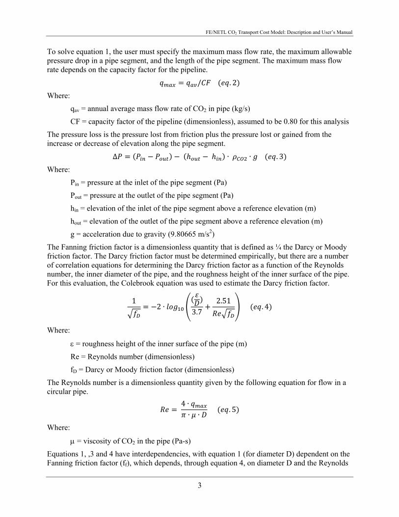
To solve equation 1, the user must specify the maximum mass flow rate, the maximum allowable pressure drop in a pipe segment, and the length of the pipe segment. The maximum mass flow rate depends on the capacity factor for the pipeline.

/ . 2

Where:

qav = annual average mass flow rate of CO2 in pipe (kg/s)

CF = capacity factor of the pipeline (dimensionless), assumed to be 0.80 for this analysis

The pressure loss is the pressure lost from friction plus the pressure lost or gained from the increase or decrease of elevation along the pipe segment.

∆ ∙ ∙ . 3

Where:

Pin = pressure at the inlet of the pipe segment (Pa)

Pout = pressure at the outlet of the pipe segment (Pa)

hin = elevation of the inlet of the pipe segment above a reference elevation (m)

hout = elevation of the outlet of the pipe segment above a reference elevation (m)

g = acceleration due to gravity (9.80665 m/s2)

The Fanning friction factor is a dimensionless quantity that is defined as ¼ the Darcy or Moody friction factor. The Darcy friction factor must be determined empirically, but there are a number of correlation equations for determining the Darcy friction factor as a function of the Reynolds number, the inner diameter of the pipe, and the roughness height of the inner surface of the pipe. For this evaluation, the Colebrook equation was used to estimate the Darcy friction factor.

12 ∙

3.72.51

. 4

Where:

= roughness height of the inner surface of the pipe (m)

Re = Reynolds number (dimensionless)

fD = Darcy or Moody friction factor (dimensionless)

The Reynolds number is a dimensionless quantity given by the following equation for flow in a circular pipe.

4 ∙∙ ∙

. 5

Where:

= viscosity of CO2 in the pipe (Pa-s)

Equations 1, ,3 and 4 have interdependencies, with equation 1 (for diameter D) dependent on the Fanning friction factor (ff), which depends, through equation 4, on diameter D and the Reynolds


4

number (Re). The Reynolds number depends on diameter D (see equation 5). Thus, to determine the diameter, an iterative procedure is needed. The following procedure was used for this evaluation.

Step 1: Provide an initial guess for the diameter: Dcur

Step 2: Calculate the Reynolds number using Dcur in equation 5

Step 3: Calculate fD using equation 4. Equation 4 is an implicit equation and is solved using the Newton-Raphson method

Step 4: Calculate a new value for the diameter, Dnew, using equation 1

Step 5: Calculate the relative difference between the two estimates for the diameter

∆ . 6

Step 6: If the relative difference ΔD is less than 10-6, then the two values are considered to have converged, and Dnew is used as the minimum inner diameter needed for the pipeline. If the relative difference ΔD is greater than or equal to 10-6, then Dcur is set equal to Dnew, and the procedure returns to step 2.

McCoy and Rubin (2008) utilized a similar procedure; however, they began with an energy balance on the pipe segment and developed the following equation for the inner diameter of the pipe. McCoy and Rubin (2008) indicated that their derivation was adapted from that provided in Mohitpour et al. (2003).

64 ∙ ∙ ∙ ∙ ∙ ∙

∙ ∙ ∙ ∙ 2 ∙ ∙ ∙ ∙

.

. 7

Where:

R = universal gas constant (8.314 m3-Pa/K-mol)

M = molecular weight of CO2 (44.01x10-3 kg/mol)

Zave = compressibility factor for CO2 (dimensionless)

Tave = average temperature of CO2 in the pipeline (K), assumed to be the ground temperature (about 285 K or 12 oC or 53.3 oF)

Pave = average pressure of CO2 in the pipe (Pa)

23∙

∙ . 8

Equation 7 replaces equation 1 in the above procedure for calculating the minimum inner diameter ID for a pipe.

In the above equations, the density of CO2 and the compressibility factor for CO2 are calculated using the Peng-Robinson equation of state. NETL (2014) provided the details of how the equations for the density and compressibility factor were implemented as user defined functions in Excel using Visual basic. The average pressure and average temperature in the pipeline are used to calculate the density and compressibility factor.


5

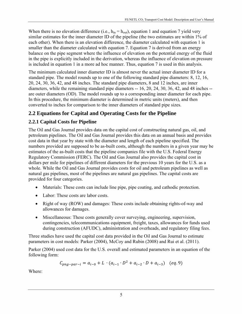
When there is no elevation difference (i.e., hin = hout), equation 1 and equation 7 yield very similar estimates for the inner diameter ID of the pipeline (the two estimates are within 1% of each other). When there is an elevation difference, the diameter calculated with equation 1 is smaller than the diameter calculated with equation 7. Equation 7 is derived from an energy balance on the pipe segment where the influence of elevation on the potential energy of the fluid in the pipe is explicitly included in the derivation, whereas the influence of elevation on pressure is included in equation 1 in a more ad hoc manner. Thus, equation 7 is used in this analysis.

The minimum calculated inner diameter ID is almost never the actual inner diameter ID for a standard pipe. The model rounds up to one of the following standard pipe diameters: 8, 12, 16, 20, 24, 30, 36, 42, and 48 inches. The standard pipe diameters, 8 and 12 inches, are inner diameters, while the remaining standard pipe diameters -- 16, 20, 24, 30, 36, 42, and 48 inches -- are outer diameters (OD). The model rounds up to a corresponding inner diameter for each pipe. In this procedure, the minimum diameter is determined in metric units (meters), and then converted to inches for comparison to the inner diameters of standard pipe sizes.

2.2 Equations for Capital and Operating Costs for the Pipeline

2.2.1 Capital Costs for Pipeline

The Oil and Gas Journal provides data on the capital cost of constructing natural gas, oil, and petroleum pipelines. The Oil and Gas Journal provides this data on an annual basis and provides cost data in that year by state with the diameter and length of each pipeline specified. The numbers provided are supposed to be as-built costs, although the numbers in a given year may be estimates of the as-built costs that the pipeline companies file with the U.S. Federal Energy Regulatory Commission (FERC). The Oil and Gas Journal also provides the capital cost in dollars per mile for pipelines of different diameters for the previous 10 years for the U.S. as a whole. While the Oil and Gas Journal provides costs for oil and petroleum pipelines as well as natural gas pipelines, most of the pipelines are natural gas pipelines. The capital costs are provided for four categories.

Materials: These costs can include line pipe, pipe coating, and cathodic protection.

Labor: These costs are labor costs.

Right of way (ROW) and damages: These costs include obtaining rights-of-way and allowances for damages.

Miscellaneous: These costs generally cover surveying, engineering, supervision, contingencies, telecommunications equipment, freight, taxes, allowances for funds used during construction (AFUDC), administration and overheads, and regulatory filing fees.

Three studies have used the capital cost data provided in the Oil and Gas Journal to estimate parameters in cost models: Parker (2004), McCoy and Rubin (2008) and Rui et al. (2011).

Parker (2004) used cost data for the U.S. overall and estimated parameters in an equation of the following form:

∙ ∙ ∙ . 9

Where:


6

Cpng-par-i = natural gas pipeline capital cost for category i (i = “mat” for materials, “lab” for labor, “ROW” for ROW & damages, or “misc” for miscellaneous) using the equation from Parker (2004) (cost in 2000 dollars)

L = length of the pipeline (mi)

D = standard diameter of pipeline (in)

ai-0, ai-1, ai-2, ai-3 = parameters that are determined by fitting the equation to the capital cost data

Using pipeline capital cost data for the U.S. as a whole from 1991 to 2003, Parker (2004) estimated values for the parameters in Equation 9 for each cost category (see Exhibit 1). The result of applying equation 9 with the parameter values in Exhibit 1 are capital costs in 2000 dollars.

Exhibit 1 Values for parameters in equation provided by Parker (2004)

Parameter Materials Labor ROW and Damages

Miscellaneous

ai-0 35,000 185,000 40,000 95,000

ai-1 330.5 343 0 0

ai-2 687 2,074 577 8,417

ai-3 26,960 170,013 29,788 7,324

McCoy and Rubin (2008) segregated the pipeline capital costs into six different regions of the U.S. using the regional definitions that the U.S. Energy Information Agency (EIA) uses when segregating natural gas pipeline costs. The division of the states into the six regions is illustrated in Exhibit 2.


7

Exhibit 2 Regions defined by EIA for segregating pipeline costs

Source: Energy Information Administration (2013)

McCoy and Rubin (2008) estimated parameters in an equation of the following form:

10 ∙ ∙ . 10

Where:

Cpng-mcc-i = natural gas pipeline capital cost for category i (i = “mat” for materials, “lab” for labor, “ROW” for ROW & damages, or “misc” for miscellaneous) using the equation from McCoy and Rubin (2008) (cost in 2004 dollars)

L = length of the pipeline (km)

D = standard diameter of pipeline (in)

ai-0, ai-reg, ai-1, ai-2 = parameters that are determined by fitting the equation to the capital cost data

The parameter ai-reg is region-specific, where “reg” can refer to “NE” (northeast), “SE” (southeast), “MW” (Midwest), “Cen” (central), “SW” (southwest) or “West” (western). Using pipeline capital cost data for different regions in the U.S. from 1995 to 2005, McCoy and Rubin (2008) estimated values for the parameters in Equation 10 for each cost category (see Exhibit 3). The result of applying equation 10 with the parameter values in Exhibit 3 are capital costs in 2004 dollars.


8

Exhibit 3 Values for parameters in equation provided by McCoy and Rubin (2008)


Miscellaneous

ai-0 3.112 4.487 3.95 4.39

ai-NE: Northeast 0 0.075 0 0.145

ai-SE: Southeast 0.074 0 0 0.132

ai-MW: Midwest 0 0 0 0

ai-Cen: Central 0 -0.187 -0.382 -0.369

ai-SW: Southwest 0 -0.216 0 0

ai-West: Western 0 0 0 -0.377

ai-1 0.901 0.82 1.049 0.783

ai-2 1.59 0.94 0.403 0.791

Rui et al. (2011) also segregated the pipeline capital costs into the six different regions of the U.S. as defined by the EIA, developed costs for constructing natural gas pipelines in Canada, and estimated parameters in an equation with a form similar to that used by McCoy and Rubin (2008):

∙ ∙ . 11

Where:

Cpng-rui-i = natural gas pipeline capital cost for category i (i = “mat” for materials, “lab” for labor, “ROW” for ROW & damages, or “misc” for miscellaneous) using the equation from Rui et al. (2011) (cost in 2008 dollars)

L = length of the pipeline (ft)

SA = cross-sectional surface area of the pipeline (i.e., πD2/4) (ft2)

ai-0, ai-reg, ai-1, ai-2 = parameters that are determined by fitting the equation to the capital cost data

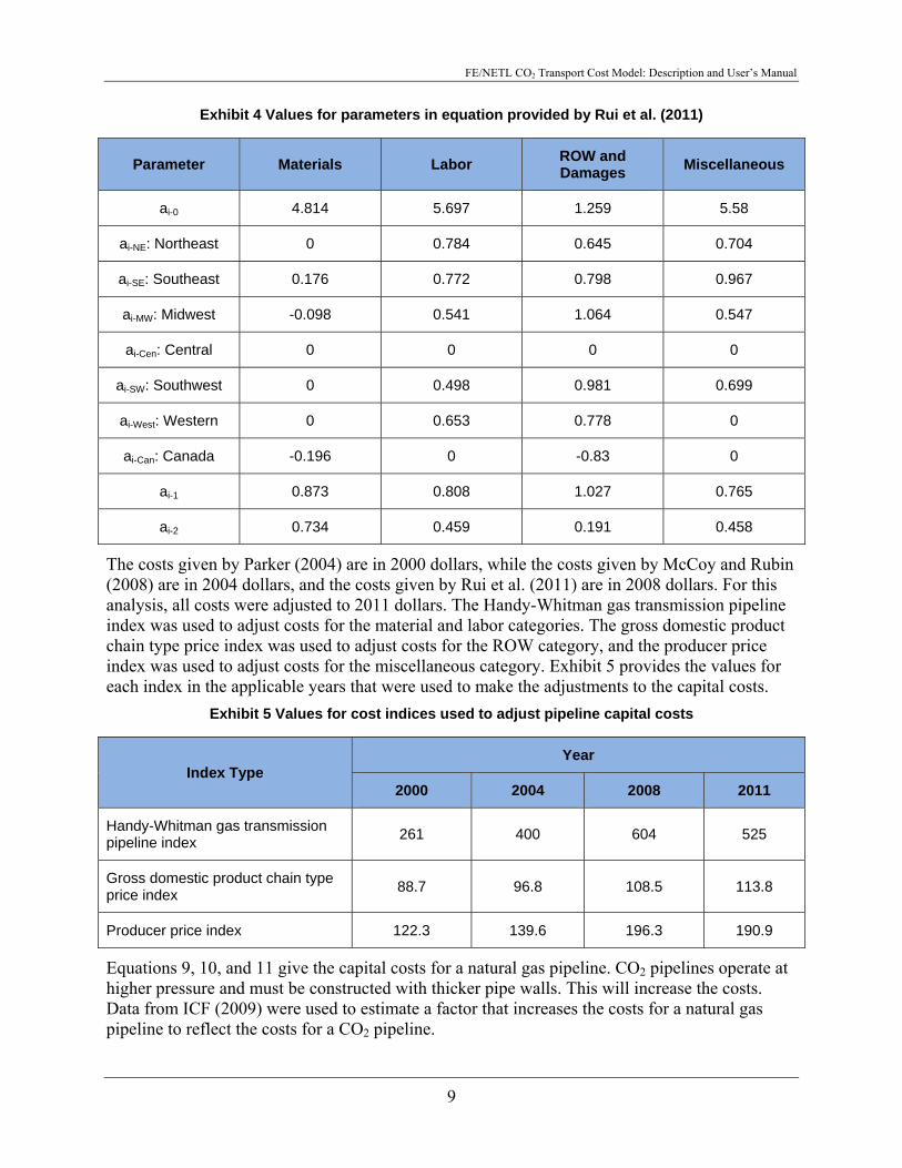
The parameter ai-reg is region-specific, where “reg” can refer to “NE” (northeast), “SE” (southeast), “MW” (Midwest), “Cen” (central), “SW” (southwest), “West” (western) or “Can” (Canada). Using pipeline capital cost data for different regions in the U.S. and Canada from 1992 to 2008, Rui et al. estimated values for the parameters in Equation 11 for each cost category (see Exhibit 4) (2011). The result of applying equation 11 with the parameter values in Exhibit 4 are capital costs in 2008 dollars.


9

Exhibit 4 Values for parameters in equation provided by Rui et al. (2011)


Miscellaneous

ai-0 4.814 5.697 1.259 5.58

ai-NE: Northeast 0 0.784 0.645 0.704

ai-SE: Southeast 0.176 0.772 0.798 0.967

ai-MW: Midwest -0.098 0.541 1.064 0.547

ai-Cen: Central 0 0 0 0

ai-SW: Southwest 0 0.498 0.981 0.699

ai-West: Western 0 0.653 0.778 0

ai-Can: Canada -0.196 0 -0.83 0

ai-1 0.873 0.808 1.027 0.765

ai-2 0.734 0.459 0.191 0.458

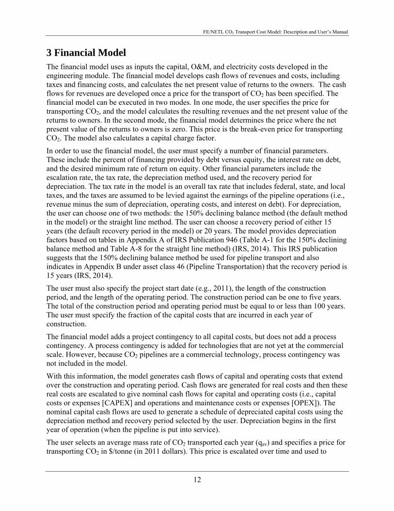
The costs given by Parker (2004) are in 2000 dollars, while the costs given by McCoy and Rubin (2008) are in 2004 dollars, and the costs given by Rui et al. (2011) are in 2008 dollars. For this analysis, all costs were adjusted to 2011 dollars. The Handy-Whitman gas transmission pipeline index was used to adjust costs for the material and labor categories. The gross domestic product chain type price index was used to adjust costs for the ROW category, and the producer price index was used to adjust costs for the miscellaneous category. Exhibit 5 provides the values for each index in the applicable years that were used to make the adjustments to the capital costs.

Exhibit 5 Values for cost indices used to adjust pipeline capital costs

Index Type Year

2000 2004 2008 2011

Handy-Whitman gas transmission pipeline index

261 400 604 525

Gross domestic product chain type price index

88.7 96.8 108.5 113.8

Producer price index 122.3 139.6 196.3 190.9

Equations 9, 10, and 11 give the capital costs for a natural gas pipeline. CO2 pipelines operate at higher pressure and must be constructed with thicker pipe walls. This will increase the costs. Data from ICF (2009) were used to estimate a factor that increases the costs for a natural gas pipeline to reflect the costs for a CO2 pipeline.


10

∙ . 12

Where:

CpCO2-x-i = capital costs for a CO2 pipeline using equation from author x (x = “par” for Parker (2004), “mcc” for McCoy and Rubin (2008) or “rui” for Rui et al. (2011)) for category i (i = “mat” for materials or “lab” for labor) (2011 dollars)

eCO2 = factor that adjusts costs of natural gas pipeline to costs for a CO2 pipeline depending on the diameter of the pipeline

= 1 for D ≤ 12 in

= 1.12 for 12 in < D ≤ 16 in

= 1.18 for 16 in < D ≤ 20 in

= 1.25 for 20 in < D

The cost adjustment factor eCO2 is only applied to the capital costs for the materials and labor categories.

2.2.2 Operating Costs for Pipelines

Bock et al. (2003) provided an annual operating and maintenance (O&M) cost for pipelines of $5,000/mi-yr in 1999 dollars. This cost was adjusted from 1999 dollars to 2011 dollars using the producer price index. The producer price index for 1999 used in the analysis was 112.6, and the value in 2011 was 190.9.

2.2.3 Capital and Operating Costs for Other Pipeline-Related Equipment

NETL (2010) provided capital costs for a CO2 surge tank of $701,600 and a pipeline control system of $94,000, with both costs in 2000 dollars. The surge tank capital cost was adjusted from 2000 dollars to 2011dollars using the Chemical Engineering index for heat exchangers and tanks. This index was 370.6 for 2000 and 657.5 for 2011. The control system capital cost was adjusted from 2000 dollars to 2011 dollars using the Chemical Engineering index for process instruments. This index was 368.5 for 2000 and 438.7 for 2011.

The annual O&M costs for these two pieces of equipment were assumed to be 4 percent of the capital costs.

2.3 Power Requirements for Booster Pumps

In order to estimate the capital and operating costs for a booster pump, the power requirement for the pump must be estimated. The power needed by a booster pump to increase the pressure of the CO2 from Ppump-in to Ppump-out is calculated as follows (from McCollum and Ogden, 2006).

∙ ∙ 10 /∙

. 13

Where:

Wpump = power requirement for the pump (kW)

Ppump-in = pressure at the inlet of the pump (equal to Pout for the pipe segment) (Pa)

Ppump-out = pressure at the outlet of the pump (equal to Pin for the pipe segment) (Pa)


11

pump = efficiency of the pump (typically around 0.75)

2.4 Equations for Capital and Operating Costs for the Booster Pumps

2.4.1 Capital Costs for Booster Pumps

The capital costs for the pump are given as follows by McCollum and Ogden (2006).

∙ . 14

Where:

Cpump = capital cost of the booster pump (cost in 2005 dollars)

Cpump-fix = fixed capital cost of the booster pump ($), a value of $70,000 in 2005 dollars from McCollum and Ogden (2006) is used in this analysis

Cpump-var = variable capital cost of the booster pump ($/kW), a value of $1,110/kW in 2005 dollars from McCollum and Ogden (2006) is used in this analysis

The capital costs are given in 2005 dollars. The pump capital cost was adjusted from 2005 dollars to 2011 dollars using the Chemical Engineering index for pumps and compression. This index was 752.5 for 2005 and 898.5 for 2011.

2.4.2 Operating Costs for Booster Pumps

The annual O&M cost for the booster pumps was assumed to be 4 percent of the capital costs.

Operating the booster pumps requires electricity, and there are costs associated with the electrical energy used. The energy used is given by the following equation.

∙ ∙ ∙ 8760 / . 15

Where:

Epump-elec = electricity used by booster pump each year (kW-hr/yr)

The cost of the electricity used is given by the following equation.

∙ . 16

Where:

Cpump-elec = cost of electricity used by booster pump each year ($/yr)

pelec = price of electricity ($/kW-hr), a price of $0.1023/kW-hr for commercial electricity users for 2011 from EIA (2013) is used in this analysis


12

3 Financial Model The financial model uses as inputs the capital, O&M, and electricity costs developed in the engineering module. The financial model develops cash flows of revenues and costs, including taxes and financing costs, and calculates the net present value of returns to the owners. The cash flows for revenues are developed once a price for the transport of CO2 has been specified. The financial model can be executed in two modes. In one mode, the user specifies the price for transporting CO2, and the model calculates the resulting revenues and the net present value of the returns to owners. In the second mode, the financial model determines the price where the net present value of the returns to owners is zero. This price is the break-even price for transporting CO2. The model also calculates a capital charge factor.

In order to use the financial model, the user must specify a number of financial parameters. These include the percent of financing provided by debt versus equity, the interest rate on debt, and the desired minimum rate of return on equity. Other financial parameters include the escalation rate, the tax rate, the depreciation method used, and the recovery period for depreciation. The tax rate in the model is an overall tax rate that includes federal, state, and local taxes, and the taxes are assumed to be levied against the earnings of the pipeline operations (i.e., revenue minus the sum of depreciation, operating costs, and interest on debt). For depreciation, the user can choose one of two methods: the 150% declining balance method (the default method in the model) or the straight line method. The user can choose a recovery period of either 15 years (the default recovery period in the model) or 20 years. The model provides depreciation factors based on tables in Appendix A of IRS Publication 946 (Table A-1 for the 150% declining balance method and Table A-8 for the straight line method) (IRS, 2014). This IRS publication suggests that the 150% declining balance method be used for pipeline transport and also indicates in Appendix B under asset class 46 (Pipeline Transportation) that the recovery period is 15 years (IRS, 2014).

The user must also specify the project start date (e.g., 2011), the length of the construction period, and the length of the operating period. The construction period can be one to five years. The total of the construction period and operating period must be equal to or less than 100 years. The user must specify the fraction of the capital costs that are incurred in each year of construction.

The financial model adds a project contingency to all capital costs, but does not add a process contingency. A process contingency is added for technologies that are not yet at the commercial scale. However, because CO2 pipelines are a commercial technology, process contingency was not included in the model.

With this information, the model generates cash flows of capital and operating costs that extend over the construction and operating period. Cash flows are generated for real costs and then these real costs are escalated to give nominal cash flows for capital and operating costs (i.e., capital costs or expenses [CAPEX] and operations and maintenance costs or expenses [OPEX]). The nominal capital cash flows are used to generate a schedule of depreciated capital costs using the depreciation method and recovery period selected by the user. Depreciation begins in the first year of operation (when the pipeline is put into service).

The user selects an average mass rate of CO2 transported each year (qav) and specifies a price for transporting CO2 in $/tonne (in 2011 dollars). This price is escalated over time and used to


13

calculate the revenue in nominal dollars that accrues to the pipeline owner in each year of operation.

The free cash flow to owners is determined using a weighted average cost of capital (WACC) methodology. The first step in the WACC methodology is to calculate the WACC using the following equation.

∙ 1 ∙ 1 ∙ . 17

Where:

WACC = weighted average cost of capital

feq = fraction of total financing that is equity

IRROEmin = minimum internal rate of return on equity

itax = tax rate (includes federal, state, and local tax rates)

idebt = interest rate on debt

The quantity (1 – itax) idebt is the tax affected cost of debt.

The second step in the WACC methodology is to calculate the earnings before interest and taxes (EBIT) in each year as follows.

. 18

The quantity COGS is the cost of goods sold, which is always zero for the pipeline operation.

The third step is to calculate the earnings before interest and after taxes (EBIAT) in each year using the following equation.

1 ∙ . 19

The fourth step is to calculate the free cash flow to owners (FCF) in each year as follows.

. 20

The change in net working capital is assumed to be zero for the pipeline operation.

The fifth step is to discount the free cash flow to owners in each year using the WACC as the discount rate, and sum the resulting discounted cash flows to yield the net present value (NPV) of the project to the owners.

An NPV for the project that is positive implies that the project returns will exceed the minimum internal rate of return on equity (IRROE) desired by the owners. Conversely, a negative NPV indicates the project returns will not satisfy the minimum IRROE desired by the owners.

The model can operate two different ways. The user can specify a price for CO2, and the model will calculate the resulting NPV and IRROE. Alternatively, the user can specify a minimum IRROE, and the model will calculate the price that needs to be charged to transport CO2 in order for the NPV for the project to be zero. When the NPV is zero, the IRROE will equal the minimum IRROE desired by the owners. This price is the break-even first-year price for CO2. It is also the break-even first-year cost for CO2.

The financial model also calculates the capital charge factor or capital recovery factor. The equation for this factor is adapted from NETL (2011a).


14

∙ / . 20

Where:

CCF = capital charge factor

pCO2 = first-year price of CO2 in 2011 dollars ($/tonne)

qCO2 = annual mass flow rate of CO2 (tonnes/yr)

Com = annual operational expenses (O&M and electricity costs) in 2011 dollars ($/yr)

TOC = total overnight capital costs (essentially total capital costs) in 2011 dollars ($)


15

4 Model Results The capital costs for natural gas pipelines were generated by the equations from Parker (2004), McCoy and Rubin (2008) and Rui et al. (2011). The breakdown of these capital costs by the four cost categories (materials, labor, right of way and damages, and miscellaneous) is also presented. The results from the model are compared to cost data from actual CO2 pipelines.

The three sets of equations for natural gas pipeline capital costs give different results, as illustrated in Exhibit 6 that presents the cost per mile for different pipeline lengths and diameters. The equations from Parker (2004) give the highest costs followed by the equations from McCoy and Rubin (2008), and then Rui et al. (2011). The equations from Parker (2004) give significantly higher costs than the other two equations. The equations from Parker (2004) do not show decreasing costs with pipeline length whereas the other two set of equations give costs that show this behavior.

Exhibit 6 Natural gas pipeline capital costs using different equations

Source: NETL


16

The breakdown of natural gas pipeline capital costs by cost category is illustrated in Exhibit 7 for 12-inch diameter pipelines, 20-inch diameter pipelines, and 30-inch diameter pipelines for the 3 different sets of equations. Labor costs are the largest component of capital costs followed by materials and miscellaneous costs. The right of way and damages cost is the smallest component of the capital costs, with the possible exception of costs generated by the equations from Rui et al. (2011) for 12-inch diameter pipelines.

Exhibit 7 Breakdown of natural gas pipeline capital costs using different equations (2011$/mi)

Source: NETL

To provide perspective on the three sets of pipeline capital cost equations to use in this analysis, a comparison was made to pipeline capital cost data from a variety of sources. The capital costs

0

200,000

400,000

600,000

800,000

1,000,000

50 100 200 300 500

Pipeline Length (mi)

12 in Pipe‐‐‐Parker Eq.

Matls Labor ROW Misc

0

100,000

200,000

300,000

400,000

500,000

600,000

700,000

50 100 200 300 500


12 in Pipe‐‐McCoy & Rubin Eq.


0

100,000

200,000

300,000

400,000

500,000

50 100 200 300 500


12 in Pipe‐‐Rui et al. Eq.


0

200,000

400,000

600,000

800,000

1,000,000

1,200,000

1,400,000

1,600,000

50 100 200 300 500


20 in Pipe‐‐Parker Eq.


0

200,000

400,000

600,000

800,000

1,000,000

1,200,000

50 100 200 300 500




0

200,000

400,000

600,000

800,000

1,000,000

50 100 200 300 500




0

500,000

1,000,000

1,500,000

2,000,000

2,500,000

50 100 200 300 500


30 in Pipe‐‐Parker Eq.


0

200,000

400,000

600,000

800,000

1,000,000

1,200,000

1,400,000

1,600,000

50 100 200 300 500




0

200,000

400,000

600,000

800,000

1,000,000

1,200,000

1,400,000

50 100 200 300 500





17

for a CO2 pipeline per inch (diameter) and mile (length) including contingency range are as follows for the different sets of equations.

Parker (2004): $85,000/in-mi (12 in pipe) to $120,000/in-mi (42 in pipe)

McCoy (2008): $65,000/in-mi (50 mile long pipe) to $46,000/in-mi (500 mile long pipe)

Rui (2011): $50,000/in-mi (50 mile long pipe) to $35,000/in-mi (500 mile long pipe)

The capital costs per inch-mile using the equations from Parker (2004) increase with increasing diameter but are relatively insensitive to the length of the pipeline. The capital costs per inch-mile using the equations from McCoy and Rubin (2008) increase somewhat with increasing diameter but decrease with increasing pipeline length. The capital costs per inch-mile using the equations from Rui et al. (2011) show the same type of behavior as the equations from McCoy and Rubin (2008).

These costs were compared to contemporary pipeline costs quoted by industry experts, such as Kinder-Morgan and Denbury Resources. Exhibit 8 details typical rule-of-thumb costs for various terrains and scenarios as quoted by a representative of Kinder-Morgan at the Spring Coal Fleet Meeting in 2009 (Lane, 2009). It is not known if these rule-of thumb estimates include contingencies. As shown, the costs using the equations from Parker (2004) are on the high end of this range, while the costs using the equations from McCoy and Rubin (2008) fall on the low end of this range, and the costs using the equations from Rui et al. (2011) tend to fall below this range.

Exhibit 8 Kinder-Morgan pipeline cost metrics (Lane, 2009)

Terrain Capital Cost

($/inch-diameter/mile)

Flat, Dry $50,000

Mountainous $85,000

Marsh, Wetland $100,000

River $300,000

High Population $100,000

Offshore (150’-200’ depth) $700,000

A further comparison was made to cost data for two Denbury CO2 pipelines. The first is the Green pipeline with the following characteristics.

Location: Southeast United States

Pipeline length: 314 miles

Pipeline diameter: 24 inches

CO2 flow capacity: 42,320 tonnes/day, assumed to be maximum daily flow, which translates to annual average flow of 12.6 million tonnes/yr


18

Capital cost: About 660 million dollars according to trade journals

About 884 million dollars excluding capitalized interest according to the annual report

Status: Completed around 2010

Assuming the capacity factor is 80 percent for this pipeline, the FE/NETL CO2 Transport Cost Model determines that a 24-inch pipeline of this length would need 2 pumps. The capital cost for this project is estimated by the model to be as follows.

Using Parker eq.: 740 million dollars

Using McCoy eq.: 435 million dollars

Using Rui eq.: 370 million dollars

The result using the Parker equations (2004) exceeds the value in trade journals but is less than the value in the annual report. The results from the McCoy and Rubin (2008) and Rui et al. (2011) equations are significantly less than both published capital costs.

The second CO2 pipeline is the Greencore pipeline with the following characteristics.

Location: Wyoming

Pipeline length: 232 miles

Pipeline diameter: 20 inches

CO2 flow capacity: 38,280 tonnes/day, assumed to be maximum daily flow, which translates to annual average flow of 11.2 million tonnes/yr

Capital cost: About 285 million dollars according to trade journals

About 135 million dollars for second half of project according to annual report

Status: Completed in 2012 or 2013

Assuming the capacity factor is 80 percent for this pipeline, the FE/NETL CO2 Transport Cost Model determines that a 20-inch pipeline of this length would need 4 pumps. The capital cost for this project is estimated by the model to be as follows.

Using Parker eq.: 430 million dollars

Using McCoy eq.: 170 million dollars

Using Rui eq.: 135 million dollars

The result using the Parker equations (2004) exceeds the value in trade journals. The results from the McCoy and Rubin (2008) and Rui et al. (2011) equations are less than the published capital costs.

These results indicate that the equations from Parker (2004) and McCoy and Rubin (2008) give costs that are closest to published CO2 pipeline costs. The equations from Parker (2004) tend to give costs on the high side, while the equations from McCoy and Rubin (2008) tend to give costs on the low side.


19

5 User’s Manual The FE/NETL CO2 Transport Cost Model is implemented in an Excel spreadsheet.

5.1 Overview of Spreadsheet

The spreadsheet used to implement the FE/NETL CO2 Transport Cost Model has an introductory sheet, two main sheets, and additional sheets that provides useful information but are not critical to the functioning of the model.

The sheet “READ_ME_FIRST” is the introductory sheet. It provides a brief overview of the model and a brief description of the sheets in the spreadsheet file. This sheet also has the BSD 1 open source software license.

The sheets “Main” and “Eng Mod” are the sheets where all the actual calculations are performed. The contents of these two sheets are described in the remainder of Section 5.

The sheet “PL Pressure Relation” provides information from ICF International (2009) on pressures in natural gas and CO2 pipelines (which are generally higher) and how capital costs for CO2 pipelines need to be increased to accommodate the higher pressures.

The sheet “Cost Indices” provides tables of cost indices used to adjust all costs to a common basis of 2011 dollars.

5.2 Inputs

The inputs to the model are specified in either the “Main” sheet or the “Eng Mod” sheet. In these two sheets, any cell that is an input cell is highlighted in orange.

“Main” sheet. The “Main” sheet is divided into 8 tables with Tables 2 and 3 requiring inputs from the user (although default values are provided in the sheet for all parameters). Table 2 requires the following inputs, with the default value presented in parentheses.

Financial parameters

o Percent equity (50% from NETL [2011b] for low-risk investor-owned utility)

o Cost of equity or minimum IRROE (12% from NETL (2011b) for low-risk investor-owned utility)

o Cost of debt or interest rate on debt (4.5% from NETL (2011b) for low-risk investor-owned utility)

o Total effective tax rate (includes federal, state, and local taxes) (38% from NETL [2011b] for low-risk investor-owned utility)

o Escalation rate (3% from NETL [2011b] for low-risk investor-owned utility)

o Project contingency factor, which is applied to all capital costs (from NETL [2011a], a project contingency in the range of 15 to 30% is recommended for the level of detail provided by the cost equations used in the model; since the miscellaneous cost category in the pipeline capital costs includes contingency [and some taxes], the lower value of 15% is specified as the default)

o Depreciation method, either DB150 for 150% declining balance method (the default method) or SL for straight line method


20

o Recovery period for depreciation, either 15 years (the default recovery period) or 20 years

o Calendar year for the start of the project (e.g., 2011)

o Duration of construction in years (can be up to 5 years with a default of 3 years from NETL [2013])

o Duration of operation in years (must be less than 95 years with a default of 30 years from NETL [2013])

Operational characteristics

o Annual average mass flow of CO2 transported in the pipeline (3.2 million tonnes/yr from NETL [2013]); note: maximum daily flow of CO2 is annual average mass flow of CO2 divided by 365 days/yr to convert this to a daily mass flow rate and then divided again by the capacity factor

o Capacity factor (80% from NETL [2013])

o Length of pipeline (62.14 mi or 100 km from NETL [2013])

o Inlet pressure for pipeline (2,200 psig from NETL [2013]) and outlet pressure for pipeline (1,200 psig from NETL [2013])

o Change in elevation from inlet to outlet of pipeline; if outlet is at a higher elevation, the change is positive (0 ft.)

o Equations to use for calculating capital costs for pipeline (specify one of the following):

PARKER for the equations from Parker (2004)

MCCOY for the equations from McCoy and Rubin (2008)

RUI for the equations from Rui et al. (2011)

o Region of United States or Canada pipeline (specify one of the following):

NE (northeast US)

SE (southeast US)

MW (Midwest US)

Cen (central US)

SW (southwest US)

West (western US)

Can (Canada)

Note: The equations of Parker (2004) have no regional component and the equations of McCoy and Rubin (2008) do not have costs for Canada.

Table 3 provides a link between the “Main” sheet, where the financial model resides, and the capital costs and operating expenses which are calculated in the “Eng Mod” sheet. In Table 3, the


21

user must specify the fraction of each capital cost that is incurred during each year of construction.

“Eng Mod” sheet. The “Eng Mod” sheet is divided into 4 sections. In Section 1, a variety of engineering calculations are performed. In particular, the pipe diameter is determined (Section 1.6) and the power requirement for the pump is determined (Section 1.7). The primary inputs to Section 1 are:

Temperature of the ground where pipes are buried (53 oF)

Pump efficiency (75% from McCollum and Ogden [2006])

Method for calculating the minimum pipe diameter:

o 0 for McCollum and Ogden (2006)

o 1 for MIT (2009)

o 2 for McCoy and Rubin (2008) (2 is default)

In Section 2, capital costs are estimated. The primary cost inputs here are the natural gas pipeline capital costs, which are calculated by one of the three sets of equations, the surge tank, the pipeline control system, and the pump costs, all of which are discussed in Section 2. Other inputs are the indices, presented in Section 2, used to adjust costs to the common basis of 2011 dollars.

In Section 3, annual operating expenses are estimated.

Section 4 lists references cited in the sheet.

5.3 Running the Model

The model is run from the “Main” sheet, which, as stated earlier, has 8 tables.

Table 1 provides a summary of output from the model and also provides the means for running the model.

Tables 2 and 3 are principally used to provide inputs (discussed previously in this report).

Table 4 provides escalation factors for calculating the nominal value of cash flows and discount factors for calculating the present value of cash flows.

Table 5 provides cash flows for capital costs and operating expenses. The cash flows are first determined in real dollars and then escalated to nominal dollars. The nominal cash flows for capital costs are used to determine a depreciation schedule utilizing straight line depreciation.

Table 6 provides cash flows for revenues. The cash flows are first determined in real dollars and then escalated to nominal dollars.

Table 7 provides the returns to owners using the weighted average cost of capital methodology discussed in Section 3. The free cash flow to owners is first determined in nominal dollars and is then discounted to present value dollars.

Table 8 calculates the capital charge factor using the methodology discussed in Section 3.

After the inputs described in the previous section have been specified, the model can be run in four different ways.


22

Note: In the discussion below the term “blank cell” means a cell devoid of any characters, even spaces. The cell cannot have blank spaces in it, because Excel treats blank spaces as characters. The term “blank out a cell” means to make a cell empty or “blank.” To “blank out a cell,” click on the cell and hit the delete key to empty or blank out the contents of the cell.

Method 1 - Determine the net present value for a pipeline project:

In the most straight forward use of the model, the user specifies in Table 1A the price that will be charged to transport CO2 in the pipeline (cell E10), the length of the pipeline (cell E14) and the number of pumps required over the length of the pipeline (cell E12). The spreadsheet then determines the pipeline diameter (cell E18) needed to transport CO2 the specified distance and calculates the net present value of cash to owners (cell E19) and the rate of return on the weighted debt and equity (cell E20). These values are displayed under the “Key Outputs” section of Table 1A. This method is appropriate when the user knows the length of the pipeline and the market price for transporting CO2. This method allows the user to see if a particular pipeline project under market conditions is profitable (i.e., has a positive net present value).

Method 2 - Break-even first-year price for specified pipeline length and number of pumps:

In some cases, the user will want to determine the break-even first-year price for transporting CO2 in a pipeline of a specified length with a specified number of pumps.

o To determine this, the user will need to run a macro. Before running the macro, the user needs to specify in Table 1A the length of the pipeline (cell E14) and the number of pumps required over this length (cell E12). The user must also blank out cell I12 in the “number of pumps” list in Table 1B (i.e., the cell in Table 1B enclosed by a thick, black border) and blank out cell P12 in the “Length of pipeline” list in Table 1C (i.e., the cell in Table 1C enclosed by a thick, black border).

o The user starts the macro by clicking the button labeled “Solve for Break-even First Year Price for Transporting CO2 in $/tonne.”

o When the macro is finished running, the macro reports the break-even first-year price for transporting CO2 in cell E10 of Table 1A.

o The macro determines the break-even first-year price by repeatedly changing the price in cell E10 until the net present value of cash to owners in cell E19 is zero. This is accomplished by using Excel’s goal seek capability. The calculated break-even first year price for CO2 may be a value with several digits after the decimal point. The macro rounds up this price to the nearest cent for reporting purposes.

Method 3 - Optimal number of pumps for single specified pipeline length:

In many cases, the user will want to determine the number of pumps for a single pipeline length that gives the lowest break-even first-year price for transporting CO2.

o To determine this, the user will need to run a macro. Before running the macro, the user needs to list the number of pumps they desire results for in Table 1B. Table 1B provides space for up to 21 “number of pumps.” The “number of


23

pumps” must be listed in increasing order in this table, but the list does not need to start with 0 or be in steady increments (e.g., the list of 1, 2, 3, 4, 5, 10, 15, 20, 25, 50 is acceptable). The list must start with cell I12 in Table 1B, enclosed by a thick, black border. The list must end with a blank cell or the 21st cell in the list.

o The user must blank out cell P12 in the “Length of pipeline” list in Table 1C, the cell enclosed by a thick, black border.


o When the macro is finished running, the macro reports results in Table 1B for each “number of pumps” listed. In Table 1A, the macro displays the number of pumps in cell E12 that gives the lowest break-even first-year price for all the “number of pumps” evaluated. The macro displays in cell E10 in Table 1A the break-even first-year price for transporting CO2 for this optimal “number of pumps.”

o The macro determines the optimal number of pumps using the following process. The macro calculates the break-even first-year price for transporting CO2, assuming that there are no pumps, and repeats this calculation for 1 pump, then 2 pumps, and so on until the largest “number of pumps” in Table 1B is reached. In other words, the macro starts with 0 for the “number of pumps” and increases this value by increments of 1 until it reaches the maximum “number of pumps” in the list in Table 1B. For a specified number of pumps, the break-even first-year price is determined by repeatedly changing this price until the net present value of cash to owners is zero. This is accomplished by using Excel’s goal seek capability. The calculated break-even first-year price for CO2 may be a value with several digits after the decimal point. The macro rounds up this price to the nearest cent for reporting purposes. The macro keeps track of the number of pumps that gives the lowest break-even first-year price. The macro displays results in Table 1B only for the listed values of “number of pumps.”

Method 4 - Optimal number of pumps for multiple pipeline lengths:

In some cases, the user will want to determine the cheapest combination of pipe diameter and number of pumps for a series of pipe lengths (Table 1C). Once again, the term “cheapest” means the combination of pipe diameter and number of pumps for a specified pipeline length that gives the lowest break-even first-year price of CO2.

o To determine this, the user will need to run a macro. Before running the macro, the user needs to list the number of pumps they desire results for in Table 1B. Table 1B provides space for up to 21 “number of pumps.” The “number of pumps” must be listed in increasing order in this table, but the list does not need to start with 0 or be in steady increments (e.g., the list of 1, 2, 3, 4, 5, 10, 15, 20, 25, 50 is acceptable). The list must start with cell I12 in Table 1B, enclosed by a thick, black border. The list must end with a blank cell or the 21st cell in the list.

o The user also needs to list the lengths of pipelines (in miles) for which they desire results. This list goes in Table 1C. Table 1C provides space for up to 41 “lengths of pipelines.” The “lengths of pipelines” can be listed in any order that the user


24

desires (e.g., the list of 62, 25, 50, 1000, 100 is acceptable). The list must start with cell P12 in Table 1C, enclosed by a thick, black border. The list must end with a blank cell or the 41st cell in the list.


o When the macro is finished running, the macro reports results in Table 1C for each of the pipeline lengths listed. The results in Table 1C are for the number of pumps that gives the lowest break-even first-year price for the specified pipeline length. Table 1C includes the break-even first-year price in the base year (i.e., 2011), the break-even first-year price escalated to the first year of the pipeline project, and the break-even first-year price escalated to the first year of pipeline operation. The number of pumps and the pipeline diameter corresponding to this break-even first-year price are also presented in Table 1C. Results are reported in Table 1A and Table 1B for the last pipeline length listed in Table 1C. Table 1B presents break-even first-year prices for the “number of pumps” listed. If the optimum number of pumps listed in the last entry in in Table 1C is not in the list of “number of pumps” then the specific results in the last entry in Table 1C will not be found in Table 1B. However, the price of CO2 (cell E10), number of pumps (cell E12) and pipeline length (cell E14) provided in Table 1A are the same as the values found in the last entry in Table 1C.

o The macro determines the optimal number of pumps for each pipeline distance using the following procedure.

The macro sets the pipeline length in cell E14 in Table 1A to the first pipeline length in Table 1C. As in Method 3, the macro then calculates the break-even first-year price for transporting CO2, assuming there are no pumps, and repeats this calculation for 1 pump, then 2 pumps, and so on until the largest “number of pumps” in Table 1B is reached. In other words, the macro starts with 0 for the “number of pumps” and increases this value by increments of 1 until it reaches the maximum “number of pumps” in the list in Table 1B. For a specified number of pumps, the break-even first-year price is determined by repeatedly changing this price until the net present value of cash to owners is zero. This is accomplished by using Excel’s goal seek capability. The calculated break-even first-year price for CO2 may be a value with several digits after the decimal point. The macro rounds up this price to the nearest cent for reporting purposes. The macro keeps track of the number of pumps that gives the lowest break-even first-year price.

The macro then goes to the next pipeline length in Table 1C and repeats the process outlined in the previous bullet for the new pipeline length. This process is repeated until all the pipeline lengths listed in Table 1C have been evaluated.


25

6 References

Bock, B., Rhudy, R., Herzog, H., Klett, M., Davison, J., de la Torre Ugarte, D., et al. (2003).

Economic Evaluation of CO2 Storage and Sink Enhancement Options. TVA Public Power

Institute.

Bureau of Labor Statistics. (2013). Producer Price Indexes. Retrieved from United States

Department of Labor, Bureau of Labor Statistics: http://www.bls.gov/ppi/

Chemical Engineering. (2013). Chemical Engineering's Plant Cost Index. Northbrook, IL:

Chemical Engineering.

Energy Information Agency (EIA). (2013a). About Natural Gas Pipelines. Retrieved 2013, from

http://www.eia.gov/pub/oil_gas/natural_gas/analysis_publications/ngpipeline/regional_de

f.html

Energy Information Agency (EIA). (2013b). Table 5.3. Average Retail Price of Electricity to

Ultimate Customers: Total by End-Use Sector, 2003 - June 2013 (Cents per

Kilowatthour). Retrieved 2013, from

http://www.eia.gov/electricity/monthly/epm_table_grapher.cfm?t=epmt_5_3

Heddle, G., Herzog, H., & Klett, M. (2003). The Economics of CO2 Storage. LFEE 2003-003

RP, Laboratory for Energy and the Environment, Massachusetts Institute of Technology.

ICF International. (2009). Developing a Pipeline Infrastructure for CO2 Capture and Storage:

Issues and Challenges. Report Number F-2009-01: The INGAA Foundation, Inc.

Internal Revenue Service (IRS). (2014). How to Depreciate Property. Publication 946. January

28, 2014.

Lane, J. (2009). Operating Experience with CO2 Pipelines. EPRI Coal Fleet for Tomorrow:

General Technical Meting. Houston, TX: EPRI.

McCollum, D., & Ogden, J. (2006). Techno-Economic Models for Carbon Dioxide Compression,

Transport, and Storage & Correlations for Estimating Carbon Dioxide Density and

Viscosity. UCD-ITS-RR-06-14, Institute of Transportation Studies, University of

California at Davis.


26

McCoy, S., & Rubin, E. (2008). An Engineering-economic Model of Pipeline Transport of CO2

with Application to Carbon Capture and Storage. International Journal of Greenhouse

Gas Control, 2, 219-229.

MIT. (2009). Carbon Management GIS: CO2 Pipeline Transport Cost Estimation. Carbon

Capture and Sequestration Technologies Program, Massachusetts Institute of

Technology.

Mohitpour, M., Golshan, H., & Murray, A. (2003). Pipeline Design and Construction. New

York, NY: ASME Press.

NETL (2014). Properties of Supercritical Carbon Dioxide as Functions of Pressure and

Temperature Implemented in Visual Basic. In preparation.

NETL. (2010). Quality Guidelines for Energy System Studies: Estimating Carbon Dioxide

Transport and Storage Costs. DOE/NETL-2010/1447; Pittsburgh, PA: National Energy

Technology Laboratory.

http://netldev.netl.doe.gov/file%20library/research/energy%20analysis/coal/qgesstranspo

rt.pdf

NETL. (2011a). Quality Guidelines for Energy System Studies: Cost Estimation Methodology for

NETL Assessments of Power Plant Performance. DOE/NETL-2011/1455; Pittsburgh,

PA: National Energy Technology Laboratory. http://www.netl.doe.gov/energy-

analyses/pubs/QGESSNETLCostEstMethod.pdf

NETL. (2011b). Recommended Project Finance Structures for the Economic Analysis of Fossil-

Based Energy Projects. DOE/NETL-2011/1489; Pittsburgh, PA: National Energy

Technology Laboratory. http://www.netl.doe.gov/energy-

analyses/pubs/ProjFinanceStructures.pdf

NETL. (2013). Quality Guidelines for Energy System Studies: Carbon Dioxide Transport and

Storage Costs in NETL Studies. DOE/NETL-2013/1614; Pittsburgh, PA: National Energy

Technology Laboratory. http://www.netl.doe.gov/energy-

analyses/pubs/QGESS_CO2T%26S_Rev2_20130408.pdf

Parker, N. (2004). Using Natural Gas Transmission Pipeline Costs to Estimate Hydrogen

Pipeline Costs. UCD-ITS-RR-04-35, Institute of Transportation Studies, University of

California at Davis.


27

Rui, Z., Metz, P., Reynolds, D., Chen, G., & Zhou, X. (2011, July 4). Regression Models

Estimate Pipeline Construction Costs. Oil and Gas Journal, 109(27).

Whitman, Requardt, and Associates. (2013). The Handy-Whitman Index of Public Utility

Construction Costs. Baltimore, MD: Whitman, Requardt, and Associates LLP.

1

www.netl.doe.gov

Pittsburgh, PA • Morgantown, WV • Albany, OR • Sugar Land, TX • Anchorage, AK

(800) 553-7681

David Morgan [email protected]

Timothy Grant [email protected]

Date post:	25-Jun-2018
Category:	Documents
Upload:	dangtuyen
View:	246 times
Download:	4 times

FE/NETL CO Transport Cost Model: Description and … Library/Research/Energy Analysis... · FE/NETL...

Documents