1 Final Report on Macroeconomic Policy Simulations for the 14 th Finance Commission By NIPFP Team * 1. Introduction Global financial crisis and the expansionary fiscal policy measures, including the fiscal stimulus in the post-Crisis period, initiated in the Union Budget 2008-09 have led to higher fiscal deficits, much higher than those specified in the FRBM act, 2003. While those policies have helped in restraining further slowdown in the economy and helped in recovery in the two subsequent years, the nature of stimulus packages 1 , which are largely irreversible in nature, appeared to have resulted in macroeconomic instability. As long term consequences of such policy measures, Indian economy is currently experiencing higher fiscal deficits, with slowdown in growth and a higher inflation rates. In order to revert back to the fiscal consolidation path, the 13 th Finance Commission revised the road map. As per the revised targets, Indian economy should achieve a fiscal deficit target of 5.4 per cent by 2014-15 while the debt-GDP ratio should be brought down to 68 per cent 2 . However, such targets were subject to some major assumptions on the exogenous factors such as external sector recovery and on the assumption of elimination of revenue deficit by 2014-15. As it turned out, the fragile recovery in the global growth and failure in reducing revenue deficit as per the revised fiscal consolidation path has made the feasibility of achieving the fiscal targets as suggested by the 13 th Finance Commission almost impossible. In 2012-13, the economy experienced a sharp slowdown with higher inflation and unsustainable current account deficits, with higher fiscal deficits. It has become necessary to review the fiscal deficit targets as prescribed by the 13 th Finance Commission. Given the domestic and global environment, the Kelkar Committee (2012) * This revised report is prepared by NIPFP team consisting of N R Bhanumurthy, Sukanya Bose, Parma Devi Adhikary, and Abhishek Kumar. Swayamsiddha Panda has contributed in the initial phase of the work. The team would like to thank Prof VN Pandit for his insightful comments on the model framework. The draft report was presented to the 14 th Finance Commission. The authors would like to thank the Commission for their comments and suggestions on the earlier version. 1 See Mundle et al, 2011 2 Mundle, et al, 2010, showed that such fiscal targets are consistent with reasonably higher and stable growth.
Transcript
1
Final Report on
Macroeconomic Policy Simulations for the14th Finance Commission
By
NIPFP Team*
1. Introduction
Global financial crisis and the expansionary fiscal policy measures, including the fiscalstimulus in the post-Crisis period, initiated in the Union Budget 2008-09 have led tohigher fiscal deficits, much higher than those specified in the FRBM act, 2003. Whilethose policies have helped in restraining further slowdown in the economy and helped inrecovery in the two subsequent years, the nature of stimulus packages1, which arelargely irreversible in nature, appeared to have resulted in macroeconomic instability.As long term consequences of such policy measures, Indian economy is currentlyexperiencing higher fiscal deficits, with slowdown in growth and a higher inflation rates.
In order to revert back to the fiscal consolidation path, the 13th Finance Commissionrevised the road map. As per the revised targets, Indian economy should achieve a fiscaldeficit target of 5.4 per cent by 2014-15 while the debt-GDP ratio should be broughtdown to 68 per cent2. However, such targets were subject to some major assumptionson the exogenous factors such as external sector recovery and on the assumption ofelimination of revenue deficit by 2014-15. As it turned out, the fragile recovery in theglobal growth and failure in reducing revenue deficit as per the revised fiscalconsolidation path has made the feasibility of achieving the fiscal targets as suggestedby the 13th Finance Commission almost impossible.
In 2012-13, the economy experienced a sharp slowdown with higher inflation andunsustainable current account deficits, with higher fiscal deficits. It has becomenecessary to review the fiscal deficit targets as prescribed by the 13th FinanceCommission. Given the domestic and global environment, the Kelkar Committee (2012)
* This revised report is prepared by NIPFP team consisting of N R Bhanumurthy, Sukanya Bose, ParmaDevi Adhikary, and Abhishek Kumar. Swayamsiddha Panda has contributed in the initial phase of thework. The team would like to thank Prof VN Pandit for his insightful comments on the modelframework.The draft report was presented to the 14th Finance Commission. The authors would like to thank theCommission for their comments and suggestions on the earlier version.1 See Mundle et al, 20112 Mundle, et al, 2010, showed that such fiscal targets are consistent with reasonably higher and stablegrowth.
2
revised and extended the fiscal deficit targets to 2016-173. Since then, the Governmenthas been trying to contain the fiscal deficits as per the revised targets. However, thereappears to be a slippage on the sub-targets such as revenue deficit. For instance, as perthe revised targets, the revenue deficit target for 2014-15 should have been 2 per centcompared to the Budget estimate of 2.9 per cent. At the same time there seems to beslippage on the growth assumption as well4. Such slippage on most of the indicatorscalls for revisiting of the fiscal deficit targets and suggest the conditions under whichone can achieve the multiple objective of fiscal consolidation with stable growth.
With this background, this study attempts to review the macro-fiscal linkages over the14th Finance Commission period of 2015-19 with the help of consistent macroeconomicframework for India. In the next section, some discussion on the revised NIPFPMacroeconomic Policy Simulation Model (MPSM) theoretical model is provided. Herethe approach is largely the Klein-Goldberger framework that follows structuralmacroeconometric method. In section-III databases and methodology used is discussedbriefly. Following this, estimated model is presented in section-IV. In section-V, basedon the assumptions on the exogenous variables, the model is simulated for both in-sample and out of sample. Diagnostic checking in terms of in-sample forecastperformance and error behaviour is undertaken to establish the robustness of the model.As the purpose is to provide some policy options for the 14th Finance Commission, threepolicy issues are discussed in section-VI. Simulation exercises are discussed in section-VII followed by the conclusion section.
II. Model Specification for the revised NIPFP Macroeconomic PolicySimulation Model
Real Sector Block
The real sector of the economy has been disaggregated into four Sectors: Agriculture,Industry, Services and Infrastructure. The forces of demand and supply impact the priceand output determination differently in the four sectors.5
The four sectors are defined as per the NAS classification by economic activity.
(a) Agriculture includes agriculture, forestry and fishing (industry group 1).(b) Industry includes mining & quarrying (industry group 2) and manufacturing
(industry group 3).
3 See the “Report of the Committee on Roadmap for Fiscal Consolidation: 2012”,http://finmin.nic.in/reports/Kelkar_Committee_Report.pdf. But these targets are only for CentralGovernment.4 Kelkar Committee (2012) assumes a nominal GDP growth of 15 per cent for 2014-15 against the UnionBudget assumption of 13.4 per cent.5 Also, there are differences in respect to fiscal variables. While agricultural incomes are outside thedirect tax net, the other sectors, particularly industrial sector, bears the burden of taxation. Publicinvestment is crucial for all the productive sectors; infrastructure growth depends on fiscal policysupport.
3
(c) Services include trade, hotels and restaurants (industry group 6), finance,insurance and real estate (industry group 8) and community and social services(industry group 9).
(d) Infrastructure includes electricity, gas and water (industry group 4), construction(industry group 5) and transport, storage and communication (industry group 7).
Agriculture
All macro-models on the Indian economy have conceptualised the agriculture sector as asupply constrained sector with accumulation of capital constraining the level of valueadded. Krishnamurty, Pandit and Mahanty (2004) cast the relationship in terms ofproductivity of land. Yield per acre is a function of net fixed capital stock per acre andtotal agricultural credit per acre of land. The latter can be interpreted as the availabilityof working capital per unit of land.
To capture the effect of technology on capital productivity in agriculture, Sachdeva andGhosh, 2009 have used area under HYV to total cropped area. Higher the area underHYV, higher the productivity of capital stock. Bhide and Parida (2009) postulate thathigher value addition of agricultural products in agro-processing and allied sectorsraises yield of agricultural production6.
Most other models do not address the agricultural productivity explicitly. Kar andPradhan (2009) determine real output as a function of capital stock and exogenouslydetermined rainfall variable. Srivastava et al (2012) add to the specification of Kar andPradhan by introducing the extent of irrigated area to total area as a determinant ofoutput. Another complementary variable that releases supply bottlenecks in agricultureis infrastructure (power, road and other transport, storage). Murty and Soumya (2006)find that infrastructure output has a significant positive impact on agricultural output.
In models where the agriculture sector has been further disaggregated, relative pricesacross commodity groups have played a significant role (Bhide and Parida, 2009;Krishnamurty, Pandit and Mahanty, 2004). These models do not find a significantlypositive price response of total agricultural output for the Indian economy.
We postulate the real agricultural output to be supply determined with productiondependent on net capital stock in agriculture and deviation of actual from normalrainfall. While the structural component of real agricultural output is a function of realcapital stock at the end of the previous period, the cyclic component would depend uponthe performance of rain, an exogenous variable. To bring in the price response ofproduction, minimum support price (MSP) is added as an explanatory variable.7
6 The variables, however, are not statistically significant in the estimated equation.
7 Net irrigated area and the area under HYV (as a proportion to total cropped area) have been stagnantover the last few years, and therefore were not included in the model specification. Institutional creditto meet the working capital needs of the agriculture sector affects real agricultural output. However,
4
1) ZYFtAGRI at FC = f(ZNKt-1
AGRI, RAIN, MSP)
ZYFtAGRI : Real agricultural GDP at factor cost
ZNKtAGRI: Real net capital stock in agriculture
RAIN: deviation of actual from normal rainfall (EXOGENOUS)MSP: minimum support price (POLICY variable)
A set of identities link investments to net capital stock in agriculture. Addition to capitalstock in agriculture between period t and t-1 takes place through net investment inperiod t (equation 2). Gross investment adjusted for depreciation is net investment(equation 3). Depreciation is assumed to be exogenous for the model.
2) ZNKtAGRI = ZNIt
AGRI + ZNKt-1AGRI
3) ZGI tAGRI = ZNIt
AGRI + DepreciationtAGRI
ZNItAGRI: Real net capital formation in agriculture
ZGItAGRI: Real gross capital formation in agriculture
DepreciationtAGRI: Depreciation of capital stock in agriculture (EXOGENOUS)
Nominal gross investment in agriculture, derived from the real gross investment inagriculture, is the sum of gross private and public investment in agriculture.
4) GI tAGRI ≡ Pt
AGRI * ZGItAGRI ≡ GIPUt
AGRI + GIPVtAGRI
GItAGRI: Nominal gross investment in agriculture
GIPVtAGRI: Nominal gross private investment in agriculture
GIPUtAGRI: Nominal gross public investment in agriculture
PtAGRI : Price deflator of agriculture sector
The sectoral investment functions for all the sectors of the Indian economy, includingagriculture, display an accelerator relationship with output. Besides, there is strongcomplementarity with public investment in agriculture (Mani, Balachandran and Pandit,2011). Real investment in agriculture is presumed to be independent of interest ratechanges, because of the preferential treatment of the sector in credit policies. Modelslike Krishnamurty et al (2004) and Bhide and Parida (2009) have included credit growthin the private investment function, since most actors in this sector are up against supplyrationing in the credit market. Higher availability of institutional credit for the farmsector would lead to higher capital formation in agriculture
We postulate private investment to depend upon the nominal output in the agriculturesector and having complementarity with (present and past period’s) public investment inagriculture.
when introduced along with capital stock in agriculture, the variable suffers from multicollinearityproblem.
5
5) GIPV tAGRI = f(YFt
AGRI, GIPU tAGRI)
YFtAGRI: GDP at factor cost in the agriculture sector.
Public investment in agriculture is a function of capital expenditure by government(combined, Centre and States) on agriculture. All government capital expenditure doesnot flow into investment and all public investment does not come from the governmentbudget alone, since it is supplemented by investment of internal surpluses of publicsector undertakings. However, the two are closely correlated.
6) GIPU tAGRI = f(ECAP t
AGRI)
7) ECAP tAGRI ≡ a1. ECAPt
where ECAP tAGRI is capital expenditure by government in agriculture (nominal); ECAPt
is total capital expenditure by government (nominal); a1: policy determined ratio ofproportion of capital expenditure going to agriculture.8
Agricultural prices are determined by a combination of supply and demand factors. Karand Pradhan (2009) estimate a simple function with real output in agriculture andprivate disposable income for determining agricultural prices. Besides, government’sactivity in agricultural markets has an important bearing on agricultural prices. Thegovernment sets the MSP which has a positive impact on prices. The government has animportant role in determining the net availability of foodgrains through its stock-holdingoperations and public distribution system. Krishnamurty (1984) had introduced percapita net availability of food grains (net production plus change in government stocksplus net imports) to represent the supply conditions in the foodgrain market.9 Alongsidereal factors, monetary factors have been used in a few models. In Krishnamurty et al(2004), M3/GDP is a common determinant of price level in all the sectors of theeconomy.
We postulate agricultural prices to be determined by a combination of supply anddemand factors and MSP. The equation is cast in terms of change in agriculture prices.Change in agricultural prices is a function of change in MSP, change in privateconsumption demand in the economy and the cyclical component of real output ofagricultural sector.
8) d(P tAGRI) = f( d(CPR t), d(MSP), Cyc_ZYFt
AGRI)
P tAGRI: Price deflator of the agricultural sector.
CPR t: Private consumptionCyc_ZYFt
AGRI: Cyclic component of ZYFtAGRI
8 While we have attempted to relate the budgetary capital expenditure with public investment, therelation is subject to certain practical limitations. Indian Public Finance Statistics reports the capitalexpenditure of the government in terms of functional heads, whereas the National Accounts Statisticsreports public investments under economic heads. This, at times, gives rise to incongruity among thecapital expenditure and public investment numbers.9 Bhide and Parida (2009) have used net availability as a determinant of price of rice.
6
Industry:
Industrial output in any year can be seen as a product of the productive capacity of theindustrial sector and the utilization of the installed capacity, while industrial capacityutilization is mainly determined by demand side variables (Kar and Pradhan, 2009). 10
Different studies have used different sets of variables to represent the demand side: realcompensation to employees (Bhide and Parida, 2009), agricultural output andautonomous expenditure where the latter is measured as government expenditure andexports of goods and services (Kar and Pradhan, 2009), real public consumption,investment plus exports (Krishnamurty et al, 2004).
In Krishnamurty et al, 2004 real output in manufacturing is modeled as a product ofcapital stock and productivity of capital stock.11 The latter is a function of both demandside and supply side variables. The supply side variables include the real infrastructuraloutput per unit of real capital stock in the manufacturing sector to explain theproductivity of manufacturing. Two other variables on the intensity of input use inmanufacturing are the non-food agricultural output and real import of crude and othermineral oils, chemicals etc (as a proportion of real capital stock in the manufacturingsector).
Bhide and Parida (2009) introduce the effect of FDI-induced technological changes as adeterminant in the output equation. FDI in mining, quarrying and manufacturing reflectsthe impact of growing integration of the economy with the international markets throughadoption of modern technology and practices on productivity. This variable is found tobe significant.
We hypothesize a demand side specification for industrial output, given thepredominantly demand constrained nature of the sector. Industrial output in real terms ispostulated as a function of overall investment demand in the economy and exportdemand for goods in the economy where both the demand side variables are expressedin real terms. Since a large part of the industrial output is produced to meet theinvestment requirements of industry and other sectors, a slowdown in investmentdemand affects the industrial sector the maximum.
9) ZYFtINDUS = f (Xt
G/PtINDUS GIt / Pt
INDUS )
ZYFtINDUS: real output of the industrial sector at factor cost
GIt: gross total investmentXt
G: exports of goods (nominal)Pt
INDUS : price deflator of industrial goods
10 In the reduced form equation on real industrial output, capacity utilization is substituted by itsdeterminants.11 Sachdeva and Ghosh (2009) macro-consistency model use a similar approach across the three sectors(agriculture, industry and services).
7
A set of identities similar to identities (2) to (4) in the agriculture sector link net capitalstock to gross investment in the industrial sector.
Gross investment in industry is the sum of private and public investment in industry.
10) GItINDUS = GIPUt
INDUS + GIPVtINDUS
GItINDUS : gross investment in industry
GIPUtINDUS : gross public investment in industry
GIPVtINDUS : gross private investment in industry
Private investment in industry is determined by (a) monetary and credit conditions; (b)expected output growth (accelerator) (c) complementarity with public investment. Thelast of these relationships, between public investment and private investment, is an oftdebated one though there is strong evidence of the importance of public sectorinvestment to revive and sustain industrial and economy-wide growth.12 Several studieshave thus tried to empirically explore crowding in and crowding out through theindustrial investment function. In Krishnamurty et al (2004) higher gross investment(total) is supposed to affect private investment in manufacturing positively, while publicinvestment (total) along with private investment in agriculture, by competing forinvestible resources, tends to affect it adversely. The authors obtain statisticallysignificant evidence of crowding out as per the above definition. Kar and Pradhan(2009) find that the impact of public investment in industry is positive on privateinvestment in the industrial sector, but the impact of higher government consumptionexpenditure is negative. The problem with Kar and Pradhan’s specification is thepresence of a close relationship between the two independent variables – publicconsumption expenditure and public investment. As we discuss later in the FiscalBlock, higher public consumption may itself cause the capital expenditure and publicinvestment to decline given fiscal deficit targets.
We postulate private investment function in industry on the lines of Mundle et al (2011).It is an accelerator type private investment function, where private investment isassumed to depend on the cost of capital as well as the crowding in effect of publicinvestment, and the expected rate of capacity utilization. This economy-wideinvestment function in Mundle et al (2011) has been taken to be valid for the industrialsector.
11) GIPV tINDUS / YMPt = f[INTRATEt, (GIPU t
INDUS /YMP t), ZYF t-1INDUS/ C(ZYF t-1
INDUS)]
INTRATEt: lending rate by commercial banksZYF t-1
INDUS: Real output of the industrial sector in the previous period.C(ZYF t-1
INDUS): Capacity output of the industrial sector in the previous period.
12 See Chakraborty (1988) “Some current issues in economic policy” in Development Planning.
8
The rate of private investment in industry is determined by interest rate, publicinvestment rate in industry and previous years’ capacity utilization rate. C(ZYF t
INDUS)or the capacity output of the industrial sector is derived by multiplying the actual capitalstock with the inverse of the trend component of capital output ratio in the industrialsector.
12) C(ZYF tINDUS) ≡ (1/ KOR_TREND t
INDUS) * ZNKtINDUS
ZNKtINDUS: Real Net Capital Stock in Industry.
KOR_TREND tINDUS is the trend component of the capital output ratio in the industrial
sector after removing the cyclical component. This variable can be viewed asrepresentative of the industrial technology. KOR_TREND t
INDUS shows a secularlyrising trend since the mid-1990s (See appendix C, figure 2 on sectoral capital-outputratio, HP-Trend).
Gross public investment in industry is linked to budgetary capital expenditure inindustry through a link equation. And capital expenditure on industry is a fraction, a2, ofthe total capital expenditure.
13) GIPU tINDUS = f(ECAP t
INDUS)
14) ECAP tINDUS ≡ a2. ECAPt
Where ECAP tINDUS is capital expenditure by government in industry (nominal); ECAPt
is total capital expenditure by government (nominal); a2 is policy determined proportionof capital expenditure going to industry.
In contrast to agricultural prices which are determined by demand and supply conditionsafter controlling for the impact of administered pricing, industrial prices exhibit cost-plus pricing. Econometric models have thus used cost factors in the industrial pricespecification. We specify industrial price (measured as industrial price deflator) as afunction of its own past value, agricultural prices, domestic oil prices and money supply(net capital flows plus bank credit). Agricultural prices and domestic oil prices representthe cost of certain essential inputs for the industrial sector, whereas the lagged value ofindustrial prices is to capture the price stickiness. Higher net capital flows and bankcredit, used as a proxy for money supply, exerts an upward pressure on industrial prices.
15) PtINDUS = f(Pt-1
INDUS, PtAGRI, Pt
OIL, Net Capital Flowst)
PtINDUS : price of industrial goods
PtAGRI: price of agricultural goods
PtOIL: administered price of oil (POLICY variable)
Net Capital Flowst: Net international capital flows to India
16) PtOIL = f(OILPRUSDt, OILPRRATIOt)
9
OILPRUSDt: International price of Indian basket of oil imports (EXOGENOUS)OILPRRATIOt is the ratio of domestic oil price index divided by the international oilprice index in Rupee terms. This is also called the pass-through ratio. Given theinternational oil prices, higher the pass-through ratio, higher is the domestic oil price.
Services:
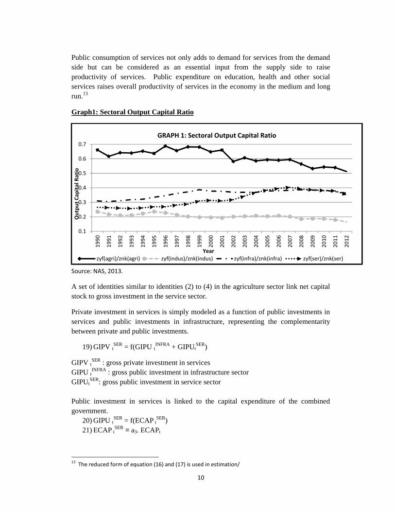
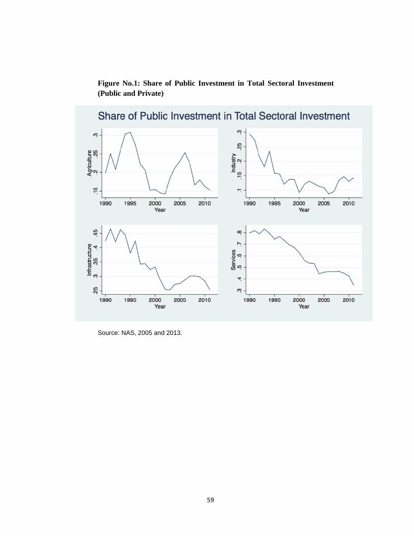
Service sector has witnessed substantial gains in productivity unlike other sectors of theIndian economy in the years since 1991 (see Graph 1 for capital productivity inservices). Rakshit (2007) notes that while there has been a decline in growth of capitalstock in services, output growth in the sector continued to be high, due to increases intotal factor productivity. In general, volume of investment required is moderate andtechnological adaption is faster and easier in the service sector.
Demand side factors have played a crucial role in raising total factor productivity inservices sector in India argues Nell (2013).Thus, most macroeconometric models havefound growth of real output in the service sector being explained by demand sidevariables. Alternate specifications to capture the importance of demand (either directlyin the output function or as a determinant of productivity of capital stock) include: realoutput of non-service sector (Krishnamurty et al, 2004, Kar and Pradhan, 2009), realcompensation to employees (Bhide and Parida, 2009); private disposable income andgovernment consumption (Srivastava et al, 2012); agricultural and industrial output andall exports, including invisibles (Sachdeva and Ghosh, 2009).
Besides the demand side factors, increase in total factor productivity in service sectorcan be explained by: (a) nature of production involving low intensity of capital andfinancial requirements, release of infrastructure bottlenecks and (b) FDI encouragedthrough favourable fiscal policies and presence of high skilled labour. Bhide and Parida(2004) find significant impact on service sector growth of supply of infrastructure andFDI in the sector.
We model the real output of the service sector as a product of productivity of capitalstock and capital stock in service sector. Service productivity in turn is explained bydomestic consumption needs (private and public) as well as external demand forservices.
17) ZYFtSER = ZNKt
SER * (Z YFtSER / ZNKt
SER)
18) ZYFtSER / ZNKt
SER = ( NXtSER/Pt
SER, CPUt +CPRt/PtSER)
ZYFtSER : real output of the service sector at factor cost
ZNKtSER: real net capital stock of the service sector
NXtSER: net exports of services
PtSER: price of services
CPRt: Private consumption demandCPUt: Public consumption demand
10
Public consumption of services not only adds to demand for services from the demandside but can be considered as an essential input from the supply side to raiseproductivity of services. Public expenditure on education, health and other socialservices raises overall productivity of services in the economy in the medium and longrun.13
Graph1: Sectoral Output Capital Ratio
Source: NAS, 2013.
A set of identities similar to identities (2) to (4) in the agriculture sector link net capitalstock to gross investment in the service sector.
Private investment in services is simply modeled as a function of public investments inservices and public investments in infrastructure, representing the complementaritybetween private and public investments.
19) GIPV tSER = f(GIPU t
INFRA + GIPUtSER)
GIPV tSER : gross private investment in services
GIPU tINFRA : gross public investment in infrastructure sector
GIPUtSER: gross public investment in service sector
Public investment in services is linked to the capital expenditure of the combinedgovernment.
20) GIPU tSER = f(ECAP t
SER)21) ECAP t
SER ≡ a3. ECAPt
13 The reduced form of equation (16) and (17) is used in estimation/
Where ECAP tSER is capital expenditure by government in services (nominal); ECAPt is
total capital expenditure by government (nominal); a3 is policy determined ratio ofproportion of capital expenditure going to services.
Unlike the industrial sector where prices follow cost-plus pricing, we hypothesize thatthe prices in the service sector are determined by demand factors. Inter-industry inputuse in the service sector is far less compared to the industrial sector or the infrastructuresector. Thus, services prices are a function of aggregate income in the economy andlagged price of services on account of price stickiness.
22) PtSER = f(Pt-1
SER, YMPt)
PtSER : Price deflator of the service sector
YMPt: nominal GDP at market price
Infrastructure:
Infrastructure sector consists of the subsectors (a) electricity, gas and water; (b)construction; and (c) transport, storage and communication. Infrastructure figures as aseparate sector in very few macro models. Infrastructure investment by the government(exogenously given) enters as a determinant in private investment functions of othersectors (RBI, 2002). Krishnamurty et al (2004) treat economic activity in infrastructuresector as supply driven. Further, they find that public infrastructure investments crowdsin private investment significantly.
We hypothesize infrastructure output as a function of real net capital stock ininfrastructure sector.
23) ZYFtINFRA = f (ZNKt-1
INFRA)
ZYFtINFRA : real output of the infrastructure sector at factor cost
ZNKt-1INFRA : real net capital stock of the infrastructure sector at the end of the previous
period.A set of identities similar to identities (2) to (4) in the agriculture sector link net capitalstock to gross investment in the infrastructure sector.
Private investment in infrastructure is dependent on the level of economic activity(accelerator relationship), interest rate (cost of borrowing) and public investment ininfrastructure (complementarity of investments).
24) GIPVtINFRA = f(GIPU t
INFRA, INTRATEt, YMPt )
GIPV tINFRA : gross private investment in infrastructure sector
GIPU tINFRA : gross public investment in infrastructure sector
12
Public investment in infrastructure is linked to the capital expenditure of the combinedgovernment.
25) GIPU tINFRA = f(ECAP t
INFRA)
26) ECAP tINFRA ≡ a4. ECAPt
Where ECAP tINFRA is capital expenditure by government on infrastructure (nominal);
ECAPt is total capital expenditure by government (nominal); a4: policy determined ratioof proportion of capital expenditure going to infrastructure sector.
Infrastructure prices (PtINFRA) is a function of its own past values and industrial
commodity price (PtINDUS), the latter capturing the inter-sectoral linkages.
27) PtINFRA = f(Pt-1
INFRA,PtINDUS)
EXTERNAL SECTOR BLOCK
With growing integration of the domestic economy with the rest of the world, there are anumber of channels through which external shocks transmit to the domestic economy.External sector is a major source of demand for sectoral output, as seen above. Highergrowth in the rest of the world causes export demand for goods and services to rise andvice-versa. On the other hand, higher domestic growth translates to higher importdemand both for intermediate use and final consumption.
Trade flows along with flows on the income account comprise the current accountbalance of the balance of payments for the economy. Current account balance (as aproportion of overall economic activity), an indicator of external balance, is a key policytarget for developing economies. Remittance income and net investment income are thetwo flows on the income account of the current account of the balance of payments.Remittance incomes increase with higher growth of advanced economies and middleeastern economies, while the net investment income is related to net capital flows. Thespecifications of the components of current account of BOPs are discussed below. 14
Export of goods is a function of World GDP, exchange rate and import weightedaverage tariff rate. The tariff rate captures the competitiveness of Indian exports (seeMundle et al, 2010).
28) XtG = f(WORLDGDPt, DUTYt, ERt)
XtG: export of goods
WORLDGDPt: world GDP (EXOGENOUS)ERt: exchange rate (EXOGENOUS)15
DUTYt: import weighted average tariff rate (EXOGENOUS)
14 The external sector block has been discussed in further detail and greater level of disaggregation inBhanumurthy et al (2014). Krishnamurthy and Pandit (1997) present a moderately disaggregative modelof India’s trade flows covering the period 1971-91.15 In Bhanumurthy et al (2014) exchange rate is endogenous, determined by the macroeconomicbalance approach.
13
29) Import of goods is a function of nominal output, international oil prices andexchange rate. Higher the international price of oil, higher is the import bill. Mt
G
= f(YMPt, ERt, OILPRUSDt )
MtG: import of goods
OILPRUSDt: oil price in US Dollars (EXOGENOUS)
Net exports of services are dependent on the level of GDP of the US, since it is themajor destination country for India’s exports of services. Merchandise exports exert apositive influence on service exports due to network effects wherein a country with highpenetration in goods market can use its networks to export services.
30) NXtSER = f(Xt
G, USGDPt)
NXtSER: net export of services
USGDPt: US GDP (EXOGENOUS)
Remittances rise with the rise in domestic interest rate and the incomes in the sourcecounties measured as the sum of GDP of Middle East and Advanced Economies.
31) REMITt = f(MEGDPt + ADVGDPt, INTRATEt)
REMITt: remittancesMEGDPt: middle east GDPADVGDPt : GDP of the advanced countriesINTRATEt : lending rates of banks
The last component of the current account of BOP is the net investment income. Netinvestment income has been deteriorating in the recent years. With persistently highcurrent account deficit, great capital inflows have been required to balance the externalaccounts, which in turn give rise to greater outflows in investment income. Netinvestment income is negatively related to net capital flows and exchange rate.
32) NETINVESTINCOMEt = f(NETCAPITALFLOWSt, ERt)
Most macro-models assume capital flows to be autonomous beyond the control ofnational authorities. Another noteworthy fact about capital flows is their procyclicalnature. We model net capital flows as a function of nominal income to reflect theprocyclical nature of capital flows. Further, credit rating is a forward looking variablethat captures the future prospects of the economy. Credit rating of a country is based onits institutional and governance effectiveness, economic structure and growth prospects,external liquidity and international investment position, fiscal performance andmonetary flexibility. By influencing the perceived investment climate, credit ratingaffects net capital flows positively. Interest rate plays a role in determining internationaldebt flows, but is found to have little influence on the aggregate net capital flows.
14
33) NETCAPITALFLOWSt = f(YMPt , CREDITRATINGt)
Current account balance (CAB) is represented by the following identity:
34) CABt = XtG - Mt
G + NXtSER +REMITt+NETINVESTINCOMEt
FISCAL BLOCK
Fiscal block has important policy levers consisting of expenditure and revenue measuresto steer the economy both from the demand side as well as supply side. This is vital inthe context of growth-inflation and fiscal imbalances, and particularly relevant to the14th Finance Commission,
Revenue receipts of the combined government comprise of direct tax revenue, indirecttax revenue and non-tax revenue. The change in direct tax revenue of government isgiven by:
35) d(DTAX)t ≡ [ 1t×d(YMP) t /YMPt-1 ]× DTAXt-1
DTAXt : Direct taxb1t : Direct tax buoyancy (POLICY variable)YMPt : Nominal income
It is assumed that the government can influence the buoyancy through adjustments intax rates and the administrative tax effort.
Similarly, the change in indirect tax revenue of government is given by:
36) d(INDTAX)t ≡ [ 2t×d(YMP) t /YMPt-1 ] × INDTAXt-1
REVEXPt : Revenue Expenditure in year tOTHERECURRt: Other Revenue Expenditure in year t.TRANSFERSt : Transfer payments by government inclusive of subsidies (Exogenous).INTERESTPAYt : Interest Payment on Debt.
OTHERECURR is the budgetary counterpart to government consumption expenditure.It includes the salaries and wages component of the government budget and is stickyupwards; it is assumed to depend on its own past values.
40) OTHERECURRt = f(OTHERECURRt-1)
Interest payments can be represented by the following identity comprising of liabilitiesat the end of the last period and rate of interest on government securities in the lastperiod.
41) INTERESTPAYt≡ LIABt-1 * ROIGSECt-1
INTERESTPAYt : Interest PaymentLIABt-1: Stock of government liabilities outstanding at the end of the previous periodROIGSECt-1: Interest rate on government securities in the previous period
Transfer payments by government inclusive of subsidies (TRANSFERS) is assumed tobe a discretionary policy variable for the model.16
Revenue Deficit (REVDEFICITt) is given by
42) REVDEFICITt≡ REVEXPt – REVRECt
Capital expenditure of the government is a crucial policy variable with important linkswith the real sector as seen in the real sector block. Bose and Bhanumurthy (2013)obtain a capital expenditure multiplier of 2.4 for the Indian economy. However, thisimportant component of government expenditure is often squeezed to make space forother kinds of expenditure. Empirically it has been found that higher the revenue deficitsmaller is the capital expenditure, given fiscal deficit (see Appendix C, Fig 4). Thus wepostulate capital expenditure to be a declining function of revenue deficit.
43) ECAPt = f(REVDEFICITt)
ECAPt : Capital Expenditure in year t
16 Transfers include all subsidies of the government. In Bhanumurthy et al (2012) oil subsidy wasendogenised and modeled as a function of oil price pass-through and international oil price. In thepresent version of the model this link is absent and subsidies are integrated with transfers, which in turnare assumed to be discretionary. The linkages of oil sector to the macroeconomy can easily beintegrated due to the flexible nature of the model.
16
Capital expenditure by the government is divided into sectoral capital expenditure.Apart from the sectoral shares, about 15-25% of total capital expenditure is defenserelated. A substantial part of this expenditure is spent on imports and has no linkagewith productive sectors in the economy.17
NDCRt : Non-Debt Capital Receipts (EXOGENOUS)d(D t) : Change in government debtd(FR t) : Change in fiscal reserves. (EXOGENOUS)
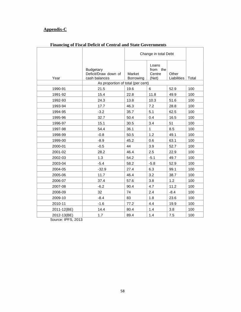
Financing of fiscal deficit occurs through change in debt, d(D)t, and change in fiscalreserves, d(FR)t. Besides debt financing part of the fiscal deficit has been met throughdrawdown of cash balances in recent times.18
Market borrowing and other borrowings of the government add to the stock of debt. 19
46) d(Dt) ≡ MBt + OBt
MBt : market borrowing of the governmentOBt : other borrowing of the government such as the proportions of small savings andprovident funds used to finance fiscal deficit (EXOGENOUS)20
Market borrowing is assumed to be a function of fiscal deficit47) MBt= f(FDt)
Note that government debt to finance fiscal deficit is a subset of total governmentliabilities, the difference ranging from 7 to 15% of GDP across years. In other words,debt is that part of total liabilities used for financing FD.
48) LIABt ≡ Dt + OLt
LIABt: Stock of government liabilities outstanding in period tOLt : Other liabilities includes liabilities on account of NSSF, State Provident Funds,Other Accounts and reserve funds not accounted for in Dt (EXOGENOUS) 21
17 Refer to appendix C, Figure no.3.18 With discontinuation of the 91-day tap treasury bills, the concept of conventional budget deficit haslost its relevance since April 1, 1997.19 Refer to appendix C, Table nos.1. Also see the Appendix B for Note on the concept of public debt andliabilities in India.20 See IPFS, 2012-13 Table 4.721 Government Debt Status Paper, MoF 2013.
17
Primary deficit (PDt) is given by
49) PDt≡ FDt -INTERESTPAYt
MONETARY BLOCK
Repo rate is a policy parameter for the Central bank. With inflation control being theprincipal objective of the RBI, repo rate (REPO) is supposed to respond to the gapbetween actual and desired inflation rate. 5% is the present desired benchmark inflationrate.
50) REPOt = f(PWPIt)-.05, REPOt-1),
The central bank responds to inflation and at the same time there is interest ratepersistence. REPO rate transmits the monetary policy signals to the economy via otherinterest rates, namely the lending rate of commercial banks (INTRATE) and interest rateon government securities (ROIGSEC).
Interest rate on government securities is assumed directly to be a function of policy rate(Repo).
51) ROIGSECt = f(REPOt)
Lending rate of commercial banks (INTRATE) is positively related to REPO and thegovernment’s market borrowing. The government being a large borrower, higher marketborrowing by the government can cause upward pressure on lending rate. Crowding outpresumes a buoyant demand for credit from the private sector.
52) INTRATEt = f(REPOt , MBt)
Disbursal of non-food bank credit by the commercial banks is assumed to be demanddetermined. Higher the investment demand in the economy, higher the demand for non-food bank credit which is met through credit expansion by banks.
53) BCt = f(GIPUt + GIPVt)
BCt: Non-food credit disbursed by commercial banks
MACROECONOMIC BLOCK
Aggregate demand in the economy is given by the following identity:
YMPt: GDP at market pricesCPRt: private consumption expenditureCPUt: public consumption expenditureGIPUt : gross public investmentGIPVt: gross private investmentXt
G: export of goodsMt
G: import of goodsNXt
SER: net export of servicesVALUABLESt : Investments on valuables and discrepancy (EXOGENOUS)
Valuables are a part of investment expenditure and consist of expensive durable goodsacquired primarily as stores of value. It is considered as exogenous for the model.Discrepancy in the national income identity has been clubbed with the valuables.
Private sector consumption is a function of private disposable income. Privatedisposable income is estimated as nominal output minus direct tax plus transferpayments and interest payments.
55) CPRt = f(YMPt-DTAXt+TRANSFERSt+INTERESTPAYt)
Public sector consumption is a function of other revenue expenditure.
56) CPUt = f(OTHECURRt)
OTHECURRt: Other revenue expenditure of the government.
Gross public and private investments are given by the following two identities:
57) GIPUt ≡ GIPU tAGRI + GIPU t
INDUS+ GIPU tSER+ GIPU t
INFRA
58) GIPVt ≡ GIPV tAGRI + GIPV t
INDUS+ GIPV tSER+ GIPV t
INFRA
Finally, the overall price deflator is derived through aggregation of sectoral pricedeflators after applying the suitable weights, w1,w2,w3 and w4.
59) Pt ≡ w1PtAGRI + w2Pt
INDUS + w3PtSER + w4Pt
INFRA
A link equation connects GDP deflator (Pt) to the wholesale price index (PWPIt).
60) PWPIt = f (Pt)
III. Database and Methodology for Estimation
The model has been estimated using annual data for the period 1991-92 to 2012-13. Insome cases, as the final NAS data for 2012-13 such as sectoral investments were notavailable at the time of estimations, the estimation is limited to 2011-12. The datadefinitions and the sources are presented in appendix-A. In terms of estimationprocedures, largely simple OLS method has been used and in some cases, when thedependent variable was found to be non-stationary, ARDL models have been used. Asthe 2008 crisis has created instability in the most of the parameters, to adjust its impact adummy variable has been introduced. Structural dummies are introduced in order to
19
capture the structural breaks in the dependent variables. To correct for autocorrelation,autoregressive (AR1) terms are introduced. However, in the estimated equations, thereare some outliers in the errors, which could be for various unexplainable reasons andmay not be explained by the theoretical variables. In order to minimise such errors andderive the robust parameters that can explain the underlying macroeconomic behaviour,outlier dummies are introduced. Such adjustments in outliers are largely similar to theError Correction Mechanism models that help in deriving underlying behaviour aftercorrecting for errors. The estimated equations are solved together by using Gauss-Seidel algorithm for the latest period, i.e., for 2009-2012. Depending on the extent oferrors in the in-sample period, the model can be used for out of sample simulations. Inthe next section, estimated regression results are discussed.
IV. Estimated Equations
Real Sector
Real Output
1) Real agricultural output has been modeled as supply constrained variable. It ispositively related to lag real capital stock, rain (% deviation from normal) andMinimum Support Price (MSP). Time trend is positive and significant. All thevariables are statistically significant and the explained variation is more than 99%.
2) Real industrial output has been modeled presuming that it’s a demand constrainedvariable. It is positively related to real investments and real export of goods. Timetrend is positive and significant. Real industrial output series has a structural break inthe year 2004 and the dummy for the same is negative and significant.
3) Real infrastructure has been modeled using both demand and supply side variable. Itis positively related to real output and capital stock. The error in the above equationfollows an AR (1) process and the AR (1) term is positive and significant.
4) Real service output has been modeled presuming that it’s a demand constrainedvariable. It is positively related to sum of private and public consumption and netexports of services.
5) Private investment in agriculture has been modeled on the lines of complementaritiesbetween private and public investment. Private investment in agriculture is positivelyrelated to public investment in agriculture, lag one of agricultural output and MSP.The results suggest that there is a crowding in situation in agricultural investment. Thepublic investment broadens the base and invites twice more private investment.
6) Private investment in Industry as fraction of nominal output is positively related topublic investment in industry as a fraction of nominal output, positively related tocapacity utilization and negatively related to interest rate. There is an evidence of publicinvestment crowding in private investment.
7) Private investment in infrastructure has been modeled on the lines ofcomplementarities between private and public investment. Private investment ininfrastructure is positively related to public investment in infrastructure and nominaloutput. The interest rate affects private investment negatively. The results suggest thatthere is a crowding in situation in infrastructural investment.
8) Private investment in service sector has been modeled on the lines ofcomplementarities between private and public investment. Private investment inservices is positively related to sum of public investment in service and infrastructure.
9) Agricultural price has been presumed to be dependent on output gap and the same hasbeen calculated using the HP- filter. Agriculture prices are influenced by demand foragricultural products (proxied by private consumption) minimum support price foragricultural products. The variables have sign as expected.
10) Industrial prices are positively dependent on the prices of inputs (agricultural and oilprices) used by industries and negatively related to the money supply proxied by sum of netcapital flows. The time trend is positive and significant. The error term follows AR(1)process and the same is significant.
14) Domestic oil price index is positively related to oil price ratio (pass-through ratio)and international crude oil prices. The oil price stickiness has been captured by lag of oilprice. Lag oil price coefficient is positive and shows a high degree of persistence in oilprices.
15) Export of goods is positively related to World GDP and exchange rate andnegatively related to import weighted average tariff rate (DUTY).The relation is asexpected by economic theory. The trend is negative and significant.
16) Import of goods is positively related to nominal output, oil prices, and is negativelyrelated to exchange rate. This relation is as expected by economic theory.
18) Remittances are positively related to interest rate and sum of GDP of Middle Eastand Advanced Economies. Higher the income in the source countries, higher theremittance flows. Exchange rate didn’t have a significant impact on remittance flows forthe sample period.
19) Net investment income is negatively related to Net capital flows and exchange rate.The error follows AR(1) process and same is found to be significant.
20) Net capital flows are positively related to nominal output and credit rating oneperiod before. Net capital flows series has Structural break in 2008 and the dummy forthe same is found to be significant.
21) Direct tax is positively related to direct tax buoyancy (elasticity of direct tax withrespect to nominal output), difference of nominal output and lag one of direct tax.
22) Indirect tax is positively related to indirect tax buoyancy (elasticity of indirect taxwith respect to nominal output), difference of nominal output and lag one of indirect tax.
24) Change in interest payment is positively related to change in government’s liability(LIAB) and weighted average rate of interest on newly issued government securities.
25) Market borrowing is positively related to fiscal deficit. With passage of time moreand more of fiscal deficit is being financed through market borrowing. The error termfollows AR(1) process and is statistically significant.
26) Repo is a policy rate and is positively relate to inflation difference (defined as actualinflation-5% target inflation) and lag one of Repo rate. The result suggests that there ispolicy rate persistence and at the same time central bank responds to inflation.
27) Interest rate which is the weighted average lending rates of banks is positivelyrelated to lagged interest rate and policy rate (Repo). As the government’s marketborrowing is one of the demand side variables in determining interest rates, growth rateof market borrowing (MB) is used. The coefficient is found to positive and significant.The market borrowing in this equation also expected to capture crowding outmechanism due to higher fiscal deficits.
29) Bank credit (BC) has been modeled as a demand determined variable and ispositively related to total investment in the economy.
BC = -283128.83 + 1.45*(IPV+IPU) +175462.85*DUMBC(-46.86) (311.42) (27.74)
Adj R2 = 0.99 DW Stat=1.73
Macroeconomic Block
30) Private sector consumption is positively related to the disposable income (defined asnominal output-direct tax +transfer payments +interest payments) and lag one of Privatesector consumption.
All the above estimated equations together with identities are solved for the recentperiod to assess the forecast performance of the whole model. The key policy variablesin solving this model include revenue and capital expenditure, tax buoyancy, minimumsupport prices, the policy interest rates, and government borrowing. The importantexogenous variables include the growth of output in OECD countries as a group as wellas in the USA and the Middle East; world oil prices; exchange rate, depreciation rates,and the rainfall index. A scenario is designed by setting the value of both the policyvariables as well as the exogenous variables. The outcome variables of interest in eachscenario include the growth rate, the inflation rate and the total liability-GDP ratio aswell as some other key macroeconomic ratios, i.e., the investment rate; the trade deficitand current account deficit relative to GDP; the tax-GDP ratio, the revenue deficit-GDPratio and the fiscal deficit-GDP ratio.
Empirical Validation
The model has been estimated using annual data for the period 1991-92 to 2012-13,taking care of time series properties. The standard diagnostic tests have also beenapplied. The model has been solved for the sample period 2009-10 to 2012-13 andvalidated for this period. The root mean square percentage errors for all the keyvariables are shown in table 1. Except for net capital inflows and trade balance, whichmodel shows slightly higher than acceptable RMSPE of 5 per cent, the rest of thevariables RMSPE is within 5 per cent. This suggests that the estimated model is robustand performs well against actual outcomes for the sample period. To see if the estimatedmodel tracks the turning points, which is another key feature of a robust model, the plotsof estimated outcome variables against their actual values in the sample period areshown in Graph-2. It may be noted that the estimated model captures many though notall of the turning points in actual outcomes.
Table 1: Historical Validation of the Model
Description RMSPE Description RMSPEPrivate Consumption 0.957 Net Exports of Services 1.541Government Consumption 1.601 Total Investment 3.436Govt. Current Expenditure 0.890 Total Government Liability 1.240Private Investment 4.336 Net Capital Inflows 5.359Public Investment 1.035 Prime lending rate 1.860Govt. Capital Expenditure 1.112 Revenue Deficit 2.521Total Govt. Revenue 1.551 GDP Deflator 1.491Fiscal Deficit 1.819 Inflation (WPI) 1.784Primary Deficit 2.405 Trade Balance 5.676Exports (only goods) 1.122 Nominal output (market price) 4.025Imports (only goods) 3.868 Real output (factor cost) 0.716Note: RMSPE=Root Mean Square Percentage Error (model generated)
26
Graph-2
Given that the estimated model is generating relatively low in-sample errors and alsocapturing majority of the turning points, this model can be used for out of samplesimulations. In the next section, the simulations would be extended upto 2019-20,which is the last year of the 14th Finance Commission period. As such the presentmodel is more of policy simulations model and less of forecasting model, here somepolicy simulations that are challenges for the Finance Commission may be attemptedand compared with the baseline case, which is a business-as-usual case. The policysimulations attempted here are i) eliminating combined revenue deficit by 2019-20; ii)targeting liability/GDP ratio of around 68 per cent, as suggested by the 13th FinanceCommission; iii) fiscal and growth outcomes in the context of external shocks (growthand price shocks); and finally iv) possibility of achieving 8 per cent GDP growth by theend of the 14th Finance Commission period. In the next section, some discussion aboutthese policy simulations and the transmission mechanisms through which the modelcould affect the variables of interest.
0
2
4
6
8
10
12
2006 2007 2008 2009 2010 2011
Actual Forecast
Real GDP growth
0
2
4
6
8
10
12
2006 2007 2008 2009 2010 2011
Inflation rate (WPI)
Actual Forecast
55
60
65
70
75
80
2006 2007 2008 2009 2010 2011
Government Liability (as ratio to GDP)
Actual Forecast
0
2
4
6
8
10
2006 2007 2008 2009 2010 2011
Combined Fiscal Deficit (as ratio toGDP)
Actual Forecast
27
VI. Challenges for Fiscal Policy in India: The Macro-Context
In this section we discuss a set of fiscal issues that are relevant for the FinanceCommission in the process of revising the fiscal consolidation path. This provides abackground and the transmission channels to the simulation exercises reported in thenext section.
(a) Targeting Revenue deficit
Fiscal rules were formally introduced in India with Fiscal Responsibility and BudgetManagement Act, 2003 (FRBMA) and FRBM Rules 2004. Elimination of revenuedeficit was among the foremost targets, along with reduction in fiscal deficit and acheck on Central Government borrowing from the RBI. Aimed at inter-generationalequity in fiscal management and debt management consistent with fiscal sustainability,limits were placed on revenue deficit and fiscal deficit targets. For instance, for thecentre, the mandate laid down included:
Eliminating revenue deficit by 2008-09 by ensuring a minimum annual reductionof 0.5 per cent or more of GDP every year from 2004-05.
Reducing fiscal deficit by at least 0.3 per cent of GDP annually from 2004-05, sothat fiscal deficit is reduced to no more than 3 per cent of GDP at the end of2008-09.
Similarly for the states, 12th Finance Commission recommended that each state enactFiscal Responsibility Legislation (FRL) which should, at the minimum, provide forelimination of revenue deficit by 2008-09 and reduction of fiscal deficit to 3 per cent ofGSDP or its equivalent defined as ratio of interest payment to revenue receipts to bebrought down to 15 per cent (pp.87, 12th FC Report). Following this pre-conditionstipulated by 12th Finance Commission, all states put in place FRL as per StateFinances. Debt-relief was provided to the states working towards fiscal consolidation.The quantum of write-off was linked to the absolute amount by which the revenuedeficit was reduced in each successive year during the award period.
Consequent to the buoyant economic growth and revenues in the years since 2003-4,fiscal rules brought about substantial improvements in fiscal balances. The performanceof the center and states vis-à-vis the fiscal rules are summarized in Table 2 and Table 3below. The global financial crisis, slowdown in domestic growth and need forcountercyclical fiscal stimulus caused a temporary pause in fiscal consolidation.
28
Table 2: Fiscal Rules and performance of Centre (per cent of GDP)
Fiscal Rules and YearRevenue Deficit[+ sign denotes deficit]
Fiscal Deficit[+ sign denotes deficit]
Primary Deficit [(-)surplus and (+) deficit]
Debt-GDPRatio
FRBM Rules (Effective from2004)
Eliminating revenue deficit by2009-10 (FRBM)
Reduce to 3 per cent of GDPby 31st March, 2010 (FRBM)
Source: 12th FC &13th FC Reports and RBI Handbook of Statistics, 2012-13Note: a) Minus (-) sign indicates ‘surplus’. P: Provisional actuals (unaudited)
b) Effective Revenue Deficit is the difference between revenue deficit and grants for creation of capital assets.c) RBI ‘s debt is the total of external liabilities and internal liabilities, where internal liabilities include other liabilities of the central government(small savings, provident
funds)d) MoF’s debt is the net of liabilities under MSS and towards NSSF not used for financing Central Government deficit.
* Effective revenue deficit is 1.8% of GDP as per 2012-13(BE).@ Data for 2014-15 (BE) are from http://planningcommission.nic.in/data/datatable/0306/table%2027.pdf
29
Table 3: Performance of States as per FC-XII and FC-XIII Targets:
2012-13(BE) -0.5 2.2 0.6 22.2 12.0Source: Indian Public Finance Statistics, 2012-13, RBI Handbook of Statistics for data on debt andReports of FC-XII and FC-XIII.Note: Minus (-) sign indicates surplus.
Subsequently, 13th Finance Commission proposed revised targets. The 13th FinanceCommission took elimination of the revenue deficit as the long term and permanenttarget for the government. The new fiscal consolidation path for the CentralGovernment entailed a decline in the revenue deficit from 4.8 per cent of GDP asprojected for the fiscal year 2009-10, to a revenue surplus of 0.5 per cent of GDP by2014-15. This allowed for acceleration in capital expenditure of the center to 3.5 percent of GDP (even more if there are disinvestment receipts). For the states, the target forfiscal deficit was 2.4% of GDP by 2014-15, with surplus on the revenue account.
The emphasis on reduction in revenue deficit and increase in capital expenditure wasrenewed by the Kelkar Committee (2012. The Kelkar Committee endorsed eliminationof effective revenue deficit rather than revenue deficit as the target. As explained inFiscal Policy Strategy Statement, Union Budget, 2012-13 effective revenue deficitreflects the structural component of imbalance in the revenue account. In a federal setup like India, large amount of transfer of resources from the Central Government takesplace to States, local bodies and other scheme implementing agencies that are mandatedto provide certain services. All of such transfers are shown as revenue/ current
30
expenditure in the books of Central Government. However, significant proportion ofsuch transfers is specifically meant for creation of capital assets which are public goodsin nature. To protect such expenditures, it was recommended that revenue deficit afternetting out the above-kind of expenditures, may be targeted. Thus, Kelkar Committee,September 2012, on the fiscal roadmap of the Central Government recommended thatfiscal deficit be reduced to 4 per cent of GDP, effective revenue deficit to be eliminatedand revenue deficit to be reduced to 2 percent of GDP by 2014-15.
Bose and Bhanumurthy (2013) based on the previous NIPFP macroeconomic model hadestimated the value of the capital expenditure multiplier to be greater than 2. Thus anyincrease in capital expenditure would cause the nominal incomes to more than double.This was the logic underpinning the fiscal consolidation path along with about 8 percent growth discussed in Mundle et al (2010).
While the emphasis on higher capital expenditure is well-placed there are genuineconcerns about compression of revenue expenditure. For instance, an importantquestion is how to treat expenditures on education on health. It has been argued thatsince development on account of health and education gets embodied in thebeneficiaries once health standards improve or educational standards are stepped up, theexpenditure incurred on these is more akin to investment and hence, it would be fair totreat it as capital expenditure. Moreover, in the absence of nurses, doctors and teachers,the capital expenditure incurred on hospital buildings or school buildings is of littleuse.22 Thus. Rakshit (2010) notes that, “given the overarching requirement of non-negative revenue balance, clubbing HRD expenditures with current ones not only leaveslittle scope for enlarging investment in human capital, but the stipulated FRBM targetsmight in all probability be met through a slowdown in HRD spending”.
(b) Debt Stabilization issues
It is generally argued that a rise in the debt-GDP Ratio is a concern as large interestpayments on public debt jeopardises the plan to raise development expenditure and alsostands in the way of provision of essential public goods. Secondly, a higher marketborrowing to finance the growing debt may lead to a higher rate of interest and thuscrowd out private investment. Further, debt might be considered problematic for fiscalsolvency. Two key factors affecting solvency are the response of primary balance (i.e.the budget balance net of interest payments on the debt) to increases in debts and thepossibility of adverse shocks. It is assumed that when debt gets very large, it may bedifficult to generate a primary balance that is sufficient to ensure sustainability, and thatshocks can push countries beyond their debt limit (Chowdhury and Islam, 2010).
There are three important concepts regarding debt-GDP ratio: stability, sustainabilityand optimality. Stability implies a constant debt ratio with time. Sustainability meansthe returns from additional borrowing should be greater than or equal to cost ofadditional borrowing. Chronic excess of government expenditure over revenue receipts
22 The 13th FC recognized this issue, but didn’t act upon it (See13th FC Report, pp.129).
31
financed through borrowing from the public is said to be sustainable if in the long runthe ratio of public debt to national income stabilizes or does not rise without limit.Optimality refers to debt level, beyond which there is a negative relationship withgrowth. We expect that beyond a certain level the debt ratio will have adverse impact ongrowth, that particular debt ratio is optimal debt.
Optimal Debt and growth: What does the empirical evidence have to say?
Some of the recent empirical literature has explored the relationship between debt-GDPand growth. An oft quoted paper by Reinhert and Rogoff (2010) seems to suggest thatbeyond 90% there may be a negative relation between debt and growth. Reinhart andRogoff, 2010 (RR henceforth) have categorized the countries in four public debtbrackets (0-30, 30-60, 60-90, and above 90% of GDP) across time and have noted thegrowth rate corresponding to the different debt levels. They calculate a compositegrowth rate for each debt category by assigning weights to countries. Composite growthrates are calculated for advanced economies and emerging market economiesseparately. The authors’ claim that the median growth declines substantially beyond90% debt-GDP level and the average growth becomes negative beyond 90% thresholdfor advanced economies. The same approach with emerging economies indicates lowermedian growth rate beyond 90%, but the average growth rate after 90% debt level is notfound to be negative. The findings of RR were countered by, Herndon, Ash, and Pollin(2013) who identified coding errors and selective weighing in RR methodology. In fact,after carrying out some formal tests, Herndon, Ash, and Pollin (2013) report thatdifferences in average GDP growth in the categories 30-60 percent, 60-90 percent, and90-120 percent cannot be statistically distinguished.
The negative relationship between growth and debt levels become more suspect as it isdriven by presence of a few strong outlier countries (with very high debt and lowgrowth combinations) and the endogenity has not been controlled for. The latter isparticularly important for developing countries. There is a strong positive empiricallyrobust relationship between a few of the economic variables which governmentexpenditure can largely influence (like initial years of schooling) and GDP growth(IMF, 2010). The growth-inhibiting effects of a given percentage increase in debt-to-GDP ratio can be easily overwhelmed by a given percentage increase in growth-promoting variables achieved through public spending. It is therefore argued that it isimportant to look at the composition of debt, instead of just focusing on the aggregatevalue of debt. (Chowdhury and Islam, 2010).
Domar (1944) put forward the sustainability condition for the debt-financing ofgovernment expenditure. According to Domar if the government finances part of itsexpenditure (amounting to a given fraction of full employment output) throughborrowing, in a growing economy public debt and government’s interest outgo asproportions of GDP will be stable in the long run provided the growth rate exceeds the
32
interest rate. The implication is that when the Domar condition is satisfied, maintenanceof full employment through debt-financing of fiscal deficits does not erode the fiscaldeficit or produce a debt-trap.
In case of India, the differential between nominal growth rate and nominal interest ratehas remained positive since 2002-3 as required by Domar’s debt sustainability condition(see Graph 2 below).
Graph 2: Differential between nominal growth rate and nominal interest rate forthe Indian economy
Source: Data for GDP from NAS, Statement 1 and rate of interest on Government securities isthe simple average of weighted average of interest rate on state government and centralgovernment securieties.The data is from, RBI, HBS,2013.
Rangarajan and Srivastava (2005) have looked at debt-stabilization wherein debt-GDPratio is unvarying across time. This requires a stricter set of condition on deficits thanrequired by Domar. The necessary and sufficient conditions for debt-stability arediscussed below:
Necessary Condition: The GDP growth rate is higher than interest rate (if the growthrate is equal to interest rate the debt ratio will rise linearly and if the growth rate islesser than interest rate the debt ratio would raise exponentially).
Sufficient Condition: Primary deficit is equal or less than the debt stabilizing level ofprimary deficit. The debt-stabilizing primary deficit is derived as under from the debt-GDP equation, Equation (1).
= + [(1+ )/(1+ )] -----------------------(1)
-0.05
0.05
0.15
0.25
1991
-92
1992
-93
199
3-94
199
4-95
199
5-96
1996
-97
1997
-98
1998
-99
1999
-00
2000
-01
2001
-02
2002
-03
2003
-04
2004
-05
2005
-06
2006
-07
2007
-08
2008
-09
2009
-10
2010
-11
2011
-12
2012
-13
Yearr g g-r
33
Where, =Debt to GDP Ratio in period t.= Primary Deficit to GDP Ratio= rate of interest= Growth rate of GDP
For debt-GDP stability we require that = . If debt-GDP is stable then we have thedebt-stabilizing primary deficit as follows from (1):
= - [(1+ )/(1+ )] = [1- (1+ )/(1+ )]
= ( - )/(1+ ) -------------------------(2)
As long as in any given year is equal to or less than for that year, the debt-GDPratio will not rise in that year compared to its level in previous year. Note thatdepends on the previous years debt-GDP ratio, growth rate and interest rate.
The debt-stabilizing primary deficit and actual primary deficit is compared with the helpof Graph 3. It can be observed from the comparison that actual primary deficit wasmore than during 1991 to 1993 and during 1996 to 2002 and for rest of the period till2012 the primary deficit is below .
The debt-GDP ratio fell during the period when the primary deficit was below . Inother words, debt-GDP ratios shows an increasing trend for more than . It isimportant to note that the debt is being defined as total liabilities of the government.(See Appendix-B: Note on the concept of public debt and liabilities in India)
Graph 3(a): Comparison of debt-stabilizing primary deficit and actual primarydeficit to GDP
Source:IPFS,2013 and NAS,2013.
-0.04
0.01
0.06
0.11
1991
-92
1992
-93
199
3-94
199
4-95
199
5-96
1996
-97
1997
-98
1998
-99
1999
-00
2000
-01
2001
-02
2002
-03
2003
-04
2004
-05
2005
-06
2006
-07
2007
-08
2008
-09
2009
-10
2010
-11
2011
-12
2012
-13
Debt-Stabilizing Primary deficit to GDP ratioActual Primary Defcit to GDP ratio
34
Grpah 3(b): Liability-GDP Ratio
Source: Liability: Table 122, RBI, HSIE. Liability refers to the total Liabilities of the combinedgovernment including internal debt, external debt and their liabilities.
The debt-GDP stability condition can also be developed using the concept of fiscal
deficit.Let us assumes fiscal deficit in period t is defined as:
= - ----------(3),
where, are Outstanding debt of government in period t and t-1
respectively.
Dividing (3) by GDP in perod t ( ) we get,
= − ∗ is the growth rate of GDP in period t.
⇒ = – ------(4)
Where, , symbolizes ratios of fiscal deficit and debt to GDP.
If = = ∗, then the debt-stabilizing fiscal deficit to GDP ratio is∗= × 1+ ---------(5)
Also, the stable debt-GDP ratio in terms of stable fiscal deficit to GDP is
∗ = ∗ ---------(6)
Numerical examples using the above relation (5) can be worked out as follows:(As %GDP)
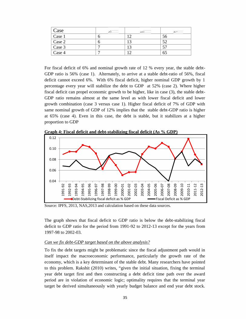
For fiscal deficit of 6% and nominal growth rate of 12 % every year, the stable debt-GDP ratio is 56% (case 1). Alternately, to arrive at a stable debt-ratio of 56%, fiscaldeficit cannot exceed 6%. With 6% fiscal deficit, higher nominal GDP growth by 1percentage every year will stabilize the debt to GDP at 52% (case 2). Where higherfiscal deficit can propel economic growth to be higher, like in case (3), the stable debt-GDP ratio remains almost at the same level as with lower fiscal deficit and lowergrowth combination (case 3 versus case 1). Higher fiscal deficit of 7% of GDP withsame nominal growth of GDP of 12% implies that the stable debt-GDP ratio is higherat 65% (case 4). Even in this case, the debt is stable, but it stabilizes at a higherproportion to GDP
Source: IPFS, 2013, NAS,2013 and calculation based on these data sources.
The graph shows that fiscal deficit to GDP ratio is below the debt-stabilizing fiscaldeficit to GDP ratio for the period from 1991-92 to 2012-13 except for the years from1997-98 to 2002-03.
Can we fix debt-GDP target based on the above analysis?
To fix the debt targets might be problematic since the fiscal adjustment path would initself impact the macroeconomic performance, particularly the growth rate of theeconomy, which is a key determinant of the stable debt. Many researchers have pointedto this problem. Rakshit (2010) writes, “given the initial situation, fixing the terminalyear debt target first and then constructing a debt deficit time path over the awardperiod are in violation of economic logic; optimality requires that the terminal yeartarget be derived simultaneously with yearly budget balance and end year debt stock.
0.04
0.06
0.08
0.10
0.12
1991
-92
1992
-93
199
3-94
199
4-95
199
5-96
1996
-97
1997
-98
1998
-99
1999
-00
2000
-01
2001
-02
2002
-03
2003
-04
2004
-05
2005
-06
2006
-07
2007
-08
2008
-09
2009
-10
2010
-11
2011
-12
2012
-13
Debt-Stabilizing fiscal deficit as % GDP Fiscal Deficit as % GDP
36
The reason is that given the prospective international scenarios and domestic parametersboth the short run and long run macro-performance of the economy depend on thenature and scale of fiscal adjustment” (p. 41).
Most debt models start off by presuming a nominal growth rate and then use it tocalculate the stable debt-ratio, with different configuration of fiscal deficit. Rangarajan& Srivastava (2005) obtain a stable debt-GDP ratio of 56% using 6% fiscal deficit toGDP ratio and nominal GDP growth of 12%.23 Based on the present and the terminalyear difference, a debt-reduction plan is suggested. It is presumed that the debtreduction or fiscal adjustment will not affect growth or other macroeconomic variables.This whole exercise leads to shifting focus from the growth to debt reduction andeconomists are aware of that as pointed by Domar (1993). “The proper solution of thedebt problem lies not in tying ourselves in to a financial straight jacket, but in achievingfaster growth of the GNP, a result which is, of course desirable by itself (Domar,1993).”
(c) Impact of external shocks on the domestic economy
With growing integration of the domestic economy with global economy through tradeand capital flows, the assessment of risks from the external shocks and its impact onmacroeconomic instability and fiscal stress becomes crucial24. Here the risks thatemanate from slower global growth and inflation risks are analysed.
Lower growth in advanced economies and the rest of the world would transmit throughlower export demand, lower export growth to the real sector. Lower external demandwould thus cause a slowdown in the economy and a deterioration of the fiscal balances,by impacting revenues in particular.
Another source of external disturbance is the international oil price shock whichtransmits through three main macro-channels to the economy. Higher international oilprices leads to higher trade imbalances and lower aggregate demand (trade channel).To the extent, higher prices cause domestic oil prices to rise, an adverse international oilprice shock would have an inflationary impact. (price channel). The fiscal decision onsubsidy influences the extent of pass-through of international prices to domestic prices.Lower the pass-through, higher the oil subsidy, which can be a drag on fiscal balances.It is however to be noted that substantial revenues accrue to the government from the oilsector and the revenues are contingent on price changes (fiscal channel).25
23 Using the relation debt-GDP ratio (56%) = fiscal deficit to GDP target (6%) *[( 1 + growth of nominalGDP at 12%)/ growth of nominal GDP at 12%]24 See Reddy (2011) for the role of risks (especially external risks) and the need for recognizing andanalyzing them for medium term growth strategy.25 See Bhanumurthy et al (2012) for details of the three channels of transmission of international oilprice shock
37
VII Some simulation results
The estimated model has been applied to assess the outcomes of three policy optionsthat are discussed in the previous section. This needs to be compared with the basecase, which is the business-as-usual case. To derive the base case upto 2019-20, onehas to extend the exogenous variables with certain assumptions. The assumptions onthe exogenous variables are as follows:
1. On the external front, the growth rates of advanced countries, Middle East andthe World GDP is assumed to grow as per the projections provided by the IMF.The import weighted average tariffs (duty) are assumed to remain at the samelevel as at present, i.e., 10%. The exchange rate, which is the crucial variable inthe external account, is assumed to be at 60. International oil prices are assumedto be constant at US$ 110 (equivalent of Indian comparable basket at INR843.12).
2. Depreciation rates at the sector level assumed to be at the 2012-13 level, whichis the latest information that is available. The capital-output ratio in theindustrial sector assumed to increase as per the trend growth. On the creditrating, given that India has a stable government at the moment, the ratingassumed to be positive.
3. Minimum support prices assumed to increase an average growth of 5 per cent. Inthe case of rainfall, except for 2014-15, which is assumed to be 10 per centbelow normal, it is assumed to be normal for the rest of the period.
4. Oil price pass-through ratio is expected to increase from the current level of 60per cent to 65 percent.
5. Share of valuables, which includes discrepancy, is assumed to be at 3.3 per centof GDP, which is the last five years average. As valuables is mostly estimatedas residual and highly volatile, modeling such behvaiour is difficult.
6. Buoyancy figures for direct and indirect taxes assumed to be at 1 and 1.382based on last three year average. Non-debt capital receipts, which is largelydisinvestment proceeds, is assumed to be at a modest level of 0.2 per cent ofGDP based on recent trends. In the case of sectoral capital expenditures, theshares in the recent year is expected to continue for the rest of the forecastperiod. Similarly, for valuables (including discrepancy) and transfers within therevenue expenditures, its share in the GDP at market price in 2012-13 isassumed for the forecast period.
Based on the above assumptions, the simulation results for the base case are presentedin table-4.
38
Table 4: Base case outcomes for 2015-16 to 2019-20 (%)
In the base case, overall GDP growth is expected to revive to over 6.5 per cent withinflation rate moderating to 6 per cent. In this case, both fiscal deficit as well as revenuedeficit tends to decline. Current account deficit also decelerate moderately to 2.3 percent. The overall recovery in the growth in the 14 Finance Commission period is drivenby the assumption on external sector growth (world growth, US growth as well asgrowth in the advance country), which is expected to revive as per the IMF projections.With this base case, some policy simulations have been carried out not only to test therobustness of the model but also address some pertinent policy questions that the 14th
Finance Commission might face in the process of establishing new fiscal policy rulesfor Centre and States.
Table 5: Base case with 7th Pay Commission Award (%)
Compared to the 13th Finance Commission, the present Commission, as part of the basecase, would need to endogenise the expected 7th Pay Commission award. Hence,keeping the assumptions on other exogenous variables as same, revised base casesimulation results are derived and is presented in table-5. However, as the 7th PayCommission is yet to submit its report and not aware of the extent of hike, a modestbroad based hike of about 15 per cent is assumed from the base case. As the awardwould be implemented from 2016-17, a one-time shock of 15 per cent is introduced in‘other current expenditure’ in 2016-17. Compared to base case, here there is an almostone per cent increase in all the fiscal parameters while the current account deficitincreases to 3.3 per cent. However, such hikes in pay structure also expected to result inslightly higher GDP growth as well as inflation with sharper rise in the shock year 2016-17.
39
Table 6: Base case with External sector risk (shock to world oil prices) (%)
To evaluate the extent of external risks that India could face, an attempt has been madeto anlayse the impact of such shocks on India. As per the present model structure,external shocks can affect the domestic economy through two ways: shocks throughglobal growth deceleration and through global price shocks. This is similar to theshocks that affected India during 2007 and 2008. While the shocks can also emanatethrough the instability in international financial markets, the present structure of themodel based on annual data has limitation to capture such shocks. The transmission ofsuch instability could be captured through net capital inflows or through net investmentincome. However, as may be noted in table-1, predictability of net capital inflows is notrobust because of its unexplained volatility.
In the first case, a shock of 10 per cent rise in the world oil prices in the initial year,2015-16, is worked out. It turned out that the impact of one time shock in world oilprices reduces GDP growth and given the fixed oil price pass-through ratio, which is apolicy decision, puts upward pressure on inflation (see table-6). With the wideningimport bill and declining growth, both fiscal deficit and current account deficit alsowidens. It was also found from the average impacts that the effect is not limited to theshock year alone.
Table 7: Base case with External sector risk (shock to world GDP) (%)
In table-7, the simulation results for a one-period shock in the World GDP growth in theinitial year, i.e., in 2015-16. For the year 2015-16, the World GDP growth has beenbrought down by half compared to the IMF projected level. It may be mentioned herethe empirical analysis suggest that in the post-crisis period, India economy appear to bemore sensitive to the shocks in the World GDP growth than to the shock in advancecountry GDP. This may suggest that in the post-crisis period, India’s trade linkage
40
would have been broadened (particularly in terms of goods trade) compared to the pre-crisis situation where India was more sensitive to advance country economic prospects.The simulation results suggest that India’s growth is highly sensitive to the externalshocks as in this case the average growth declines to 5.6 per cent compared to 6.3 percent in the base case (without 7th Pay award). But the extent of impact is larger in theyear of shock (2015-16), where the growth has sharply declined to 2.1 per cent.
2019-20 7.5 6.2 35.3 3.6 6.0 1.8 1.4 64.814th FCaverage 7.3 6.3 34.0 3.3 6.6 2.8 2.0 65.9Note: Compared to external shocks scenario, in this case 7th Pay Commission award is endogenised.
One of the most important terms of reference to the 14th Finance Commission is to“review the state of the finances, deficit and debt levels of the Union and the States,keeping in view, in particular, the fiscal consolidation roadmap recommended by theThirteenth Finance Commission, and suggest measures for maintaining a stable andsustainable fiscal environment consistent with equitable growth including suggestionsto amend the Fiscal Responsibility Budget Management Acts currently in force…”.The 13th Finance Commission has recommended the public debt as a ratio to GDP atabout 68 per cent while suggesting for a fiscal deficit target of 5.4 per cent by the end of2014-15. This was expected to be achieved through eliminating revenue deficit andincreasing the disinvestment target of around one per cent26.
As discussed earlier, while the deficit targets were already off the mark and wasreworked by the Kelkar Committee (2012), public debt target seems to have beenachieved and currently it is at 56 per cent27. However, in our view, it is pertinent totarget the total government liability, which is broader concept that includes public debt
26 Such strategy is consistent with the findings of Mundle, et.al (2011)27 One reason for this is sharp upward revision in the nominal GDP following new production functionwith base 2009-10.
41
as well as other liability. In the year 2012-13, for which latest information is available,the total liability as a ratio to GDP is at 65.43 per cent.
In the base case (with 7th Pay award) as in table-5, the total liability as a ratio to GDP isexpected to increase to close to 70 per cent by 2019-20. Here a simulation exercise iscarried to understand the policy options to bring it down to the current levels (of 65 percent). As the fiscal consolidation by principle suggest for expenditure switching fromrevenue to capital, here an attempt has been made to undertake such exercise in twostages and examine the simulation outcomes in terms of growth and other indicators28.The results are presented in tables-8 & 9.
In the first stage, public capital expenditure is exogenously increased from current levelof about 4 per cent to 4.4 per cent by keeping other exogenous variables constant. Thisincrease in public capital expenditure is allowed only from 2017-18 as the fiscal spacefor increase in capital expenditure is limited until then due to higher allocation forrevenue expenditure following 7th Pay award in 2016-17. Such policy interventionresults in higher output growth through increase in investment rate (see table-6). All thefiscal variables also show some moderate decline from the base case. However, in thiscase, there is a risk that such strategy could be inflationary as well as expand the currentaccount balance and may not be a viable policy option. In the second case, simulation iscarried by increasing capital expenditure and at the same time reducing the revenueexpenditure. The results are presented in table-9.
In the model, revenue expenditure is disaggregated into interest payments, transfers andthe other current expenditure. While interest payments and other current expendituresare largely committed expenditures, the policy option is limited to transfers (which arelargely subsidies). In 2012-13, the transfers is at 5.6 per cent of GDP compared to 4.4per cent in the pre-crisis period (2007-08) when India was close to achieving revenueneutral. Following expenditure switching policy, while transfers have been broughtdown gradually from the year 2015-16 to pre-crisis levels by 2019-20, the increases inpublic capital expenditure is allowed only from 2017-18. In such scenario, it is possibleto revert back to present level of liability of 65 per cent by 2019-20 when the publiccapital expenditure increases to 4.4 per cent. This also results in fiscal deficit of 6 percent and the revenue deficit to about 1.8 per cent of GDP. The most important here isthat such fiscal adjustments would also result in higher GDP growth compared to basecase (table-5) with almost no change in the current account deficit29.
28 In the case of India, as evidenced by Bose & Bhanumurthy (2012), such expenditure switching couldlead to ‘expansionary fiscal consolidation’.29 The model is further used to analyse the possibility of achieving 8 per cent growth by the end of 2019-20. Preliminary results suggest that, in this case capital expenditure needs to be increased further. Thisresults in decline in liability-GDP ratio to 63 per cent while fiscal deficit and revenue deficit declining to5.5 and 1.1 per cent respectively. However, in this case, current account deficit reaches to 4 per cent.
42
Revisions as per the 14th Finance Commission suggestions30
Revised assumptions on the exogenous variables based on inputs from the FinanceCommission are as follows:
1. Direct and indirect tax buoyancies are changed to 1.48 and 1.42 respectively, for2013-14 as per 2013-14(BE) and direct tax buoyancy and indirect tax buoyancyare assumed to be 1.1 from 2014-15 onwards.
2. The share of other revenue expenditure as a proportion of GDP is assumed at 13per cent instead of 13.5 per cent for 2013-14 and 2014-15. This is taken as per2013-14 (BE).
3. A lower international oil price of USD 802 per MT (instead of 843.116) hasbeen assumed for 2013-14 based on recent RBI data. From 2014-15,international oil price is assumed at USD 720 per MT which is equivalent to$100 per barrel (approx.).
Results
In the baseline scenario (Table A1), the average GDP growth is expected to be 7 percent, with inflation moderating to about 6 per cent on an average. Revival in growthwith inflation moderating, translates to an average growth of nominal output at 13.5 percent. The investment rate in the economy rises to 34 per cent by the terminal year.Besides the recovery in domestic investment, the overall recovery in growth in the 14th
Finance Commission period is driven by the assumption in external sector growth (USgrowth, other advanced country growth and world GDP growth), which is expected torevive as per the IMF projections.
The external balance deteriorates marginally owing to the higher domestic growth.Current account deficit to GDP (in percentage) is, however, contained at less than 2.5per cent of GDP, on an average. This could be largely due to assumption of lowerworld oil prices. There is an improvement in the fiscal indicators as well. Revenuebalance improves as a percentage of GDP which reduces the fiscal deficit to GDP ratio.Improvement in fiscal deficit along with higher growth is responsible for lower liability-GDP ratios by the end of the period. The assumptions of lower world oil prices as wellas slightly higher revenue buoyancy assumption appear to improve the fiscal indicators.However, the major assumption of lower Other Revenue expenditure (lower by 50 basispoints) has led to sharp decline in the fiscal indicators.
30 In this revision, major changes are undertaken in the assumptions on fiscal indicators for 2013-14 and2014-15, especially on deficits and revenue buoyancies. As there is no actual data for these years, as perthe 14 Finance Commission recommendations, here the Budgeted numbers (on both deficits as well asrevenue buoyancies) are used for these years. In our view, going by the recent trends where the actualdeficit numbers are higher than Budgeted (except in one year when there was windfall gains due tospectrum auction), such assumption itself could underestimate the fiscal numbers in the forecast period.Even the buoyancy assumption of over 1.4 is also on the higher side as such higher buoyancies areexperienced only in the pre-Crisis period.
43
Table A1: Base case outcomes for 2015-16 to 2019-20(per cent)
During the 14th Finance Commission period, the 7th Pay Commission award would beannounced. One therefore needs to endogenise the expected 7th Pay Commissionaward. Keeping the assumptions on other exogenous variables same, revised base caseis presented in Table A2. A shock of 15 per cent in the growth of other revenueexpenditures is assumed for 2016-17, the year of announcement of the award.Compared to the base case, in the revised base case, a real growth of 0.6 per cent alongwith higher inflation of 0.3 per cent is expected, on an average. However, the impact ofsuch shocks on terminal year is minimal in both growth and inflation. Current accountbalance too is projected to worsen. And so does the fiscal indicators. Revenue deficitand the fiscal deficit rise by 0.9 per cent of GDP in the revised base case compared tothe base case. Liability as a ratio to GDP is expected to increase by two percentagepoints by the terminal year.
Table A2 (SCENARIO 1) : Revised Base case with 7th pay commission Award (15per cent shock in growth of other revenue expenditure in 2016-17)
In the next scenario, public capital expenditure is increased from current level of about 4per cent to 4.4 per cent (along with the pay commission award). That is, there is anincrease in capital expenditure to GDP ratio from the prevailing level of 4 per cent ofGDP in 2016-17 to 4.4 per cent by 2019-20 in a staggered manner. This increase inpublic capital expenditure is allowed only from 2017-18 as the fiscal space for increasein capital expenditure is limited until then due to higher allocation for revenueexpenditure following 7th Pay award in 2016-17. Increase in capital expenditure of thegovernment and thereby public investment is found to be growth-enhancing.Investment rate crosses 35 per cent by 2019-20. Due to higher growth, the currentaccount deficit worsens slightly compared to the revised base case while fiscalindicators improve due to higher growth and higher revenue collections.
Note: 7th Pay Commission award is endogenised in this case.
One of the most important terms of reference to the 14th Finance Commission is to“review the state of the finances, deficit and debt levels of the Union and the States,keeping in view, in particular, the fiscal consolidation roadmap recommended by theThirteenth Finance Commission, and suggest measures for maintaining a stable andsustainable fiscal environment consistent with equitable growth including suggestions toamend the Fiscal Responsibility Budget Management Acts currently in force…”. The13th Finance Commission recommended the public debt as a ratio to GDP at about 68per cent while suggesting for a fiscal deficit target of 5.4 per cent by the end of 2014-15.This was expected to be achieved through a reduction in revenue deficit culminating inrevenue surplus of 0.5 per cent of GDP by 2014-15. While the total liability to GDPratio has remained well-within the 13th FC targets, deficits have often breached thetargeted levels. In view of the higher than targeted deficit levels, the Kelkar Committee(2012) suggested revised targets of 2 per cent and 4 per cent of GDP, respectively, forcenter’s revenue deficit and fiscal deficit to be achieved by 2014-15. It is to be notedthat the present levels of center’s revenue deficit and fiscal deficit to GDP stands at 3.26per cent and 4.62 per cent of GDP for 2013-14 (RE).31 Also, both in Scenario 1 and 2,the fiscal deficit to GDP ratio exceeds 7 per cent of GDP on an average.
The next scenario looks at the fiscal adjustments required to achieve the 13th FinanceCommission (overall, center and states) fiscal deficit targets by 2019-20. Compared tothe preceding scenario, an expenditure reduction is brought about by reduction intransfers to GDP ratio to pre-crisis level (5.6 per cent to 4.4 per cent between 2015-16and 2019-20). The reduction in transfers has been partially offset by increase in capitalexpenditure in a partial expenditure switching strategy.
Table A4 (Scenario 3): Targeting Deficit and Liability
Note: 7th Pay Commission award is endogenised in this case. The shock to capital expenditure describedin Scenario 2 has been retained.
31 For 2014-15, the Centre’s revenue deficit to GDP and fiscal deficit to GDP are budgeted at 2.94 percent and 4.13 per cent, respectively.
45
Reduction in transfers by reducing the disposable income, compresses consumption andgrowth. Inflation rate declines. As compared to scenario 2, there is improvement inexternal balance and substantial gains in fiscal balance. Liability to GDP ratio declinesto 60 per cent by the terminal year of the 14th Finance Commission.
Conclusions
In this study, an attempt has been made to understand the dynamic relationship betweenfiscal policy and macroeconomic outcomes in the case of India. With the help ofrevised NIPFP Macroeconomic Policy Simulation Model, some preliminary policysimulations that are relevant to 14th Finance Commission have been carried out. Someof those issues are endogenizing 7th Pay Commission award, targeting debt-deficits aspart of re-drawing fiscal consolidation road map, targeting higher growth, etc.
Our preliminary results suggest that while Pay Commission award indeed would resultin slightly higher growth compared to the base case, this also results in higher inflation,fiscal-revenue deficits, current account deficit as well as higher government liability.Further simulation results suggest that expenditure switching policy, which is the coreof expansionary fiscal consolidation mechanism, by increasing higher governmentcapital expenditure and reducing the government transfers could result in higher growthwith a manageable fiscal deficit of 6 per cent that also brings down the governmentliability to its present level of 65 per cent. However, the decline in current accountdeficit is only marginal due to higher growth. This higher growth with lower fiscaldeficit could be because of strong multiplier effect of government capital expenditurecompared to revenue expenditures.
While it is not clear what the 14th Finance Commission intends to target, our analysissuggests that there is enough scope for ‘expansionary fiscal consolidation’ strategythrough expenditure switching in favour of higher capital expenditure. This strategy isexpected to result in better macroeconomic outcomes. Significantly, the analysis alsosuggests that there is no clear crowding-out impact of government revenue expendituresas the interest rate channel appear to be weak in the post-Crisis period.
46
ReferencesBernheim, Douglas B (1989): ‘A Neoclassical Perspective on Budget Deficits’, Journalof Economic Perspectives, Vol 3, No 2, pp 55-72.
Bhide Shashanka and Parida (2009), ‘Impact of External Economic Environment: Anassessment using a Macroeconometric Model’, Macro-Modelling for the Eleventh FiveYear Plan of India, Planning Commission, Government of India, Academic Foundation,New Delhi.
Bhanumurthy, N. R. Sukanya Bose and Swayamsiddha Panda (2014), ‘ModelingIndia’s External Sector: Review and Some Empirics’, Margin, Vol.8, No.4, Pp.457-493.
Bhanumurthy, N R, Surajit Das, and Sukanya Bose (2012) `Oil price shock, pass-through policy and its impact on the Indian Economy’, NIPFP Working Paper No.99(March).
Bose.S & N R Bhanumurthy(2013), 'Fiscal Multipliers for India' , Working Paper No.2013-125, NIPFP, New DelhiChakravarty. S (1988), ‘Development Planning: The Indian Experience’, New Delhi,Oxford University Press, Oxford, New York.Chowdhury. A and Iyanatul Islam (2010), ‘Is there an optimal debt-to-GDP ratio?’,United Nations ESCAP.
Domar, E. D. (1944), ‘The ‘Burden’ of Public Debt and National Income’, AmericanEconomic Review, 34(4): 798-827.
Domar, Evsey D. (1993). ‘On Deficits and Debt’, American Journal of Economics andSociology 52 (4): 475-478.
GOI (2005) Report of the Twelfth Finance Commission, 2010-2015.
GOI (2010) Report of the Thirteenth Finance Commission, 2010-2015.
GOI (2012) Report of the Committee on Roadmap for Fiscal Consolidation (Chairman:Vijay Kelkar).
GOI (2013) Economic Survey, 2012-13, Ministry of Finance.
Kar, Sabyasachi and Basanta K. Pradhan (2009), ‘Shocks, Meltdowns, PolicyResponses and Feasibility of High Growth in the Indian Economy’, Macro-Modellingfor the Eleventh Five Year Plan of India, Planning Commission, Government of India,Academic Foundation, New Delhi.
Krishnamurty, K (1984), ‘Inflation and Growth: A Model India, 1961-1980’, IndianEconomic Review.
Krishnamurty, K. and V.Pandit (1997) Exchange Rate, Tariff and Trade Flows:Alternative Policy Scenarios for India, Journal of Asian Economics, Vol. 8, No.3
47
Krishnamurty, K., V.Pandit and G.Mahanty (2004), ‘Policies for Stability and GrowthExperiments with a Large and Comprehensive Structural Model for India’, EconomicPolicy Modeling for India, Oxford University Press.
Mani, Harish, G. Bhalachandran, and V Pandit (2011) Public Investment in Agriculturaland GDP Growth: Another Look at the Inter-sectoral Linkages and Policy Implications,CDE Working Paper No. 201.
Murty. K.N & A. Soumya, 2006. ‘Macroeconomic effects of public investment ininfrastructure in India,’ Indira Gandhi Institute of Development Research, MumbaiWorking Papers 2006-003, Indira Gandhi Institute of Development Research, Mumbai,India.
Mundle, Sudipto, N.R. Bhanumurthy and S. Das (2011), ‘Fiscal Consolidation withHigh Growth: A Policy Simulation Model for India’, Economic Modeling, 2011,Pp.2657-2668.
Mundle, Sudipto; M Govinda Rao and N R Bhanumurthy (2011): “Stimulus, Recoveryand Exit Policy: G20 Experience and Indian Strategy”, Economic and Political Weekly,16th July, 2011, Pp.85-94.Nagaraj, R (2013), ‘India's Dream Run, 2003-08: Understanding the Boom and ItsAftermath’, Economic and Political Weekly, Vol - XLVIII No. 20.Nell, K. S. (2012), ‘An alternative explanation of India’s growth transition: ademand-side hypothesis’, Cambridge Journal of Economics, 37, 113-141.Rakshit, M (2007), ‘Services-led Growth: The Indian Experience’, Money and Finance,3(1) February.
Rakshit, M (2010), ‘Fiscal Consolidation and Inclusive Growth: The FinanceCommission Approach’, Economic & Political Weekly, vol. xlv no 48.
RBI (2002), ‘Report on Currency and Finance’, 2000-01 (RBI Model).
Rangarajan, C. and D.K. Srivastava, ‘Fiscal Deficits and Government Debt in India:Implications for Growth and Stabilisation’, Economic and Political Weekly”, July,2005.
Reddy, Y.V (2011), ‘Prospects and Policy Challenges in the Twelfth Plan: A Commenton the Risks’, Economic and Political Weekly, June 11, Vol.XLVI No.24, pp.81-82.
Sachdeva, A.S. and P.P. Ghosh (2009), ‘A Macro Consistency Planning Model’,Macro- Modelling for the Eleventh Five Year Plan of India, Planning Commission,Government of India, Academic Foundation, New Delhi.
Srivastava, D.K, K.R Shanmugam and C.B Rao (2012), ‘A Macro-Fiscal ModelingFramework for Forecasting and Policy Simulations’, Madras School of Economics.
48
Appendix-A
Definition & Data Sources
CPR is Consumption by the Private Sector at current prices, in Rs. crores. Source isvarious issues of NAS.
CPU is Consumption by the Public Sector at current prices, in Rs. crores. Source isvarious issues of NAS.
CAPSTOCK refers to Net Capital Stock at constant prices, that is, Net Capital Stockfigures at 2004-05 prices. Net Capital Stock figures include Net Fixed Capital Stock aswell as stock of inventories, as on 31st March of the year. It is to be noted that thefigures of Capital Stock for a year correspond to the figures of the variable at thebeginning of the year. Source is various issues of NAS.
Depreciation (at Constant Prices) is the consumption of fixed capital in Rs. Crores.Source is various issues of NAS.
Debt is the sum of internal and external debt used to finance fiscal deficit. Calculatedon the basis of Table No.4.7 of IPFS, 2012-13.
Direct Tax refers to the direct taxes of the Centre and states (combined) in Rs. Crores,including taxes like corporation tax, income tax, estate duty, interest tax, wealth tax, etc.Data from IPFS, various issues, Table 1.2 Combined Revenue Receipts of the Centreand the States.
DUTY is the import weighted average tariff rate. Data from the website of the PlanningCommission of India, Data book for DCH, 2nd April, 2013.
ECAP AGRI comprises of capital expenditure on agriculture & allied services (5) andirrigation & flood control less of power projects (7-7a). Source IPFS Table 2.4.
ECAP DEF is the capital expenditure on defence (1) under non-developmentalexpenditure. Source IPFS Table 2.4
ECAP INDUSTRY comprises of capital expenditure on industry and minerals (6).Source IPFS Table 2.4
ECAP INFRA comprises of capital expenditure on border roads (2) under non-developmental expenditure, railways (1), posts & telecommunications (2), powerprojects (7a), transport & communication (8) and public works (9). Source IPFS Table2.4
ECAP SERVICES comprises of fiscal services (3), others (4) under non-developmental expenditure and social and community services (3) and generaleconomic services (4) under developmental expenditure. Source IPFS Table 2.4
49
ER is the nominal exchange rate of the Indian rupee vis-à-vis US Dollar (Rupees perunit of $, annual average). Source is RBI, DBIE
Export of Goods is export of merchandise in Rupees crores ((Table 143: KeyComponents of India’s Balance of Payments), RBI, HSIE, 2012-13.
Export of Services is Non-factor Services, Receipts in Rs. Crores. Source: HSIE,2012-13, RBI, TABLE 145.
Fiscal deficit (FD) in Rs. Crores: Combined (center and states) gross fiscal deficit.Table 4.3, IPFS, 2012-13.
Gross Capital Formation (at current prices), corresponds to total investment in thesector in Rs. Crores. Source is various issues of NAS.
Gross Capital Formation-Public (At Current Prices), corresponds to publicinvestment in the sector in Rs. Crores Source is various issues of NAS.
Gross Capital Formation-Private (At Current Prices), corresponds to privateinvestment in the sector in Rs. Crores, has been calculated residually by subtractingpublic sector gross capital formation from total gross capital formation in the sector.
Gross Capital Formation (at 2004-05 prices), corresponds to total investment in thesector in Rs. Crores. Source is various issues of NAS.
Gross Capital Formation - Public (At 2004-05 Prices), corresponds to publicinvestment in the sector in Rs. Crores. Source is various issues of NAS.
Imports of Services is Non-factor Services, Payments in Rs. Crores. Source: RBI,HSIE, Table 145: Invisibles by Category of Transactions - Rupees
Indirect Tax refers to the indirect taxes of the Centre and states (combined) in Rs.Crores, including taxes like Customs, Union excise duties, Service tax, State exciseduty, Stamp & registration fee, General sales tax, Taxes on vehicle, Entertainment tax,etc. Source: RBI, HSIE.
Interest Rate (WALR) or the Total Weighted Average Lending Rate is the weightedaverage nominal lending rate, total of all sectors. Source: Database on Indian Economy
Investment Income in Rs. crores corresponds to the net figures of Investment Incomeas given in the HSIE, 2012-13, Table 141: India's Overall Balance of Payments:Rupees.
Liabilities (LIAB) is public debt plus other liabilities of government (Centre andStates) like small savings which is not used to finance fiscal deficit. Data from RBI,HSIE, Table 122: Combined Liabilities of the Central and State Governments.
MB is net market borrowing by the center and states combined in Rs Crores.
50
Source: Table 118: Market Borrowings of the Central and States Governments. HSIE,2012-13.
MSP is the weighted average of the Minimum Support Price of paddy and wheat (in Rs.Per quintal), taking the procurement of rice and wheat as the respective weights.Source: MSP for paddy and wheat in Rs per quintal from Handbook of Statistics onIndian Economy (HSIE), RBI, Table 25: Minimum Support Price for Foodgrainsaccording to Crop Year.
Net Capital Flows refers to the Capital Account Balance, in Rs. Crores. Data from,RBI, HSIE, Table 143.
Non-Debt Capital Receipts determined residually from the Fiscal Deficit Identity.
Non-food gross bank credit in Rupees crores; Table 48: Sectoral Deployment of Non-Food Gross Bank Credit (Outstanding), RBI, HBS.
Non-Tax Revenue is revenue receipts less tax revenue.
Rainfall (% departure) refers to the percentage deviation between actual and normalrainfall, where rainfall is overall Rainfall from June-May (in millimeters).Source isAgricultural Statistics at a Glance, 2013, Table 20.3: All India Rainfall Distributionfrom 1992-93 to 2013-14.
Remittances equal net official transfers plus net private transfers, in Rs. crores. Datafrom RBI, HSIE, Table 145: Invisibles by Category of Transactions - Rupees. We haveadded the compensation of employees to it.
REPO is the RBI determined bank rate taken up to 2000-01 and repo rate thereafter.Data from Table 46, HSIE, 2012-13.
Revenue Deficit (RD) in Rs. Crores: Combined (Centre and states) revenue deficits.Source is Table 1.6 Overall Budgetary positions of The Centre and the States, IPFS,2012-13.
Revenue Receipts in Rs. crores refer to the combined revenue receipts of the Centreand the states including tax and non-tax revenue, transfer from funds and adjustmentson account of difference in figures of Centre and states transfers. Source: Data fromIPFS, various issues, Table 1.2.
Total Government Borrowing from RBI (Combined) refers to the sum of net RBIcredit to central and state governments in Rs. Crores.
Trade Balance is exports of goods and services minus imports of goods and services,in Rs. crores.
51
Transfers are the revenue expenditure of the government to the private consumptionsector in the form of transfer payments. The data to calculate transfers is obtained fromIPFS 2012-13, Table 1.3. It includes pension and other retirement benefits, relief onaccount of natural calamities (plan and non-plan), social security and welfare (plan andnon-plan), food-subsidy, fertilizer subsidy.
Other Revenue Expenditure is determined residually by subtracting Interest Paymentsand Transfers from Revenue Expenditure (ECURR).
WPI_ All Commodities at 2004-05 base (2004-05=100) is the overall WPI for theentire basket of goods covered under it. Data from Office of the Economic Advisor tothe Government of India.
YF The data for GDP at Factor Cost (Current Prices) in Rs. Crores. Source is variousissues of NAS.
YMP Refers to GDP at Market Prices (at current prices) in Rs. Crores. Source isvarious issues of NAS.
ZYF The data for GDP at Factor Cost (Constant Prices) in Rs. Crores. Source is variousissues of NAS.
ZYMP Refers to GDP at Market Prices (at 2004-05 prices) in Rs. Crores. Source isvarious issues of NAS.
52
Appendix-BA note onConcept of Public Debt and Total Liabilities in India
This note provides some discussion on the concept of public debt as adopted in India. Italso discusses the present reporting system and inconsistencies in the definitions thatare followed by different agencies. At the end, some recommendations on both conceptas well as reporting system. Since, ‘public debt’ is the most important information thatis taken seriously by the investors, rating agencies as well as the sovereigngovernments, it is felt that there is a need to address the ambiguities existing in India.
As per our understanding, total liabilities of the government include debt specified inthe Consolidated Fund of India (defined as Public Debt) as well as liabilities in thePublic Accounts. Public Debt consists of internal debt of Centre and States as well asthe external debt of Centre. Internal Debt largely consists of fixed tenure and fixedcoupon borrowings (dated securities and treasury bills) which are issued throughauction. External Debt is at present a small proportion of the overall public debt of theGovernment of India. It is largely used for financing specific projects at the Central andState levels. States are not permitted to contract external debt directly and therefore inthe existing system all external debt (even those not used for financing Central Govt.projects) are first contracted in the Consolidated Fund of India and then on-lent toStates.
There are two dimensions of public debt: one is debt in terms of stock and second, isdebt as flow. Stock of debt relates to the accumulated volume over years, net ofrepayments every year, whereas, the flow is the extent of debt financing of theconcerned year’s deficit. The flow is captured in a broad sense by the volume of grossfiscal deficit financed during the year through internal and external debt and partly byother liabilities of the government. The ‘other liabilities’ of government arise inGovernment’s accounts more in its capacity as a banker rather than as a borrower. Suchborrowings, not secured under the consolidated fund of India, are shown as part ofPublic Accounts. All liabilities, for whatever purpose they may be generated, areobligations of the government (RBI Bulletin, 1997).
Need for distinct nomenclatures
The study of public debt is important from the point of analyzing the financing of fiscaldeficit, on the other hand, total liabilities of the government is concerned with the totalpublic debt of the government both as a borrower and as a banker. Often the two notionsare used interchangeably, although the two are conceptually different. The GovernmentDebt Status Paper highlights the difference when it says “the total liabilities reported in
53
the budget documents of the Central Government need to be adjusted so that theoutstanding debt truly reflects the outcome of fiscal operations of the Centralgovernment.” (MOF, 2013; p.1) In terms of magnitude there is a vast differencebetween debt and liability. Total liability and public debt as a proportion of GDP arepresented in Graph 1B. The difference in the two series even in the latest period is asmuch as 10% of GDP.
Graph-1B: Liability-GDP and Debt-GDP Ratios
Source: Liability from RBI, HBS and debt computed as a sum of internal debt of Centre andStates’ and external debt of Centre (data taken from RBI, HBS).
As debt and liability are two different concepts, it is highly recommended that twodistinct nomenclatures should be established for debt and liability. Policy makers shouldexplicitly spell out the underlying concept while deliberating on issues of stability,sustainability, solvency or any other important aspect related to debt and liability.
Need for a consistent definition of Total Liabilities
The figure for public debt of the government (Centre + States) is given only byGovernment Debt Status Paper, MoF. The figures of total liabilities are given by RBI,IPFS and Government Debt Status Paper, MoF and the estimates differ widely. This isbecause the various sources providing data for total liability of the combinedgovernment use different definitions.
The difference in the definition of total liabilities by three different sources is shown inTable 1B:
20
40
60
80
100
1990
-91
1991
-92
1992
-93
1993
-94
1994
-95
1995
-96
1996
-97
1997
-98
1998
-99
1999
-00
2000
-01
2001
-02
2002
-03
2003
-04
2004
-05
2005
-06
2006
-07
2007
-08
2008
-09
2009
-10
2010
-11
2011
-12
2012
-13
Debt
and
Liab
ility
as p
er ce
nt o
f GDP
YearDebt-GDP Liability-GDP
54
Table 1B: Measurement of Total liability of the government (Centre and States)
Reserve Bank of India (RBI),Handbook of Statistics on theIndian Economy
Government Debt Status Paper,MoF
Indian Public FinanceStatistics (IPFS)
Total Outstanding Liabilities(TL) Includes:
Total Outstanding Liabilities(TL) Includes:
Total Outstanding Liabilities(TL) Includes:
a) Internal Liabilities of Centre a) Internal Liabilities of Centre a) Internal liabilities of Centre
b) External Liabilities of Centreat current exchange rate.
b) External Liabilities at currentexchange rate.
b) External Liabilities of Centreat historical exchange rate.
c) Total Liabilities of States c) Total Liabilities of States c) Total Liabilities of States
TL excludes: TL excludes: TL excludes:
i)Loans and advances fromCentral government to States
i) Loans and advances fromCentral government to States
i) Loans from Centre to States.
ii)Special Securities issued toNSSF
ii)Special Securities issued toNSSF
iii) State governments’investment in Centre’s treasurybills.
iii) States investment in Centre’streasury bills.
iv) Market stabilization scheme
Total Liabilities figures of IPFS are higher than the other two sources as IPFS does notfully make allowance for the inter-governmental transactions between the Centre andthe state governments.32 IPFS also considers external debt at historical exchange ratewhereas the other sources compute external debt at current exchange rate. There isbroad agreement between the RBI and MOF on the different adjustments on totalliabilities, except on MSS where there are two different view-points. RBI’s value fortotal liability is slightly higher than the Government Debt Status Paper, MoF because RBIincludes the liabilities on account of MSS under the internal debt since 2004-05.Government Debt Status Paper (MoF, July 2013) argues against the inclusion of MSSunder total liabilities definition since it is a pure monetary instrument and not aconsequence of fiscal operation.
The presence of different liability numbers based on different definitions is confusingfor researchers and policymakers. Again in terms of magnitude the differences are notinsignificant. (see Graph 2B). It is recommended that a consistent definition be used tocompute and report government liabilities.
32 See RBI, HSIE, 2013-14 Notes on Tables 122 and 237, p. 403.
55
Graph 2B: Total Liabilities as per the definition of RBI, MoF and IPFS (as %GDP)
Source: As given in Table 1B
Reporting mechanism for center and states’ liabilities
The Middle Office in Department of Economic Affairs, Ministry of Finance publishesquarterly report for public debt management beginning the first quarter of the fiscal year2010-11. It provides data for Center’s public debt. To our knowledge, there is no similarquarterly report available on states’ debt positions.
There is no uniformity in reporting mechanism of data on liabilities for Centre andStates, combined. Also between different sources the reporting periods are different.For instance, for Centre, the total liabilities figures are available for 2013-14 (RE) aswell as for 2014-15(BE) whereas only the 2013-14(BE) data is accessible for States(refer to RBI’s website). This makes any attempt at consolidation difficult. IPFS,although provides highly over-estimated numbers, provides consolidated data onliabilities for center and states but with a lag. Whereas RBI has published 2013-14(RE)numbers on liabilities, IPFS in its latest publication has given budget estimated figuresfor 2013-14, both for Centre and States. Synchronization of the reporting time wouldhelp in the compilation of debt and liability statistics. Researchers and policymakerswould benefit from updated and improved information on such crucial variables relatedto the Indian economy.
60
70
80
90
2006
2007
2008
2009
2010
2011
2012To
tal L
iabi
litie
s of C
entr
e an
d St
ates
(as %
GDP
)
Year
RBI MoF IPFS
56
Table-2B: Currently reporting pattern in India by different agencies:
Items Source Time of reportingTotal Liability RBI Annually
End September, end Decemberand annual publication of statusreport capturing one financialyear.
Public Debt Public DebtManagement, MoF
Quarterly (only for Centre)
Suggestion
From the above discussion, following suggestions may be made.
1. Conceptualization of ‘public debt’ in India that takes care of broader definitionand is relevant for understanding the country’s solvency position. The conceptalso needs to be comparable with other countries. At the moment, the existingdefinition of ‘public debt’, in our view, under-estimates and needs revision.
2. The definition of ‘public debt’ should be uniform across the differentgovernment statistical sources. Maintaining consistency and providingconsistent data may be given to one agency. At the moment RBI is undertakingsuch exercise independent of IPFS (which is published by MoF). IPFS may alsouse the same source.
3. Inconsistency in the reporting of public debt data is the most crucial issue. Asnoted above, at the moment there is no clarity on the release of the data. Giventhe importance of the public debt data, the data release should be systematic andneeds to be released atleast twice a year on pre-specified date. Further, themanagement of public debt is the responsibility of the sovereign and the lawmakers need to be aware of this. It may be suggested that both MoF and the RBI(as a data producer) may submit the consolidated public debt (including otherliabilities) to the Parliament atleast twice a year.
References for Appendix-B:
Government Debt Status Paper, Ministry of Finance, Department of Economic Affairs,New Delhi, November 2010.
Government Debt Status Paper, Ministry of Finance, Department of Economic Affairs,New Delhi, March 2012.
57
Government Debt Status Paper, Ministry of Finance, Department of Economic Affairs,New Delhi, July 2013.
India’s External Debt, A Status Report, Ministry of Finance, Department of EconomicAffairs, External debt Management Unit.
India’s External Debt As At End-September, Ministry of Finance, Department ofEconomic Affairs, External debt Management Unit.
India’s External Debt As At End-December, Ministry of Finance, Department ofEconomic Affairs, External debt Management Unit.
Indian Public Finance Statistics, Ministry of Finance, Department of Economic Affairs,Economic Division, New Delhi, 2013-14.
Handbook of Statistics on Indian Economy, Reserve Bank of India, 2013-14 and 2014-15.
Placing a Statutory Limit on Public Debt, Reserve Bank of India Bulletin, 1997.
Public Debt Management, Quarterly Report, Ministry of Finance, Budget Division,Department of Economic Affairs.
58
Appendix-C
Financing of Fiscal Deficit of Central and State Governments