FINITE ELEMENT ANALYSIS OF LEFT VENTRICLE MOTION AND MECHANICAL PROPERTIES IN THREE DIMENSIONS ABDALLAH IBRAHIM MOHAMMED HASABALLA DISSERTATION SUBMITTED IN FULFILLMENT OF THE REQUIREMENTS FOR THE DEGREE OF MASTER OF ENGINEERING SCIENCE FACULTY OF ENGINEERING UNIVERSITY OF MALAYA KUALA LUMPUR 2014
Transcript
FINITE ELEMENT ANALYSIS OF LEFT VENTRICLE
MOTION AND MECHANICAL PROPERTIES IN THREE
DIMENSIONS
ABDALLAH IBRAHIM MOHAMMED HASABALLA
DISSERTATION SUBMITTED IN FULFILLMENT
OF THE REQUIREMENTS FOR THE DEGREE OF
MASTER OF ENGINEERING SCIENCE
FACULTY OF ENGINEERING
UNIVERSITY OF MALAYA
KUALA LUMPUR
2014
UNIVERSITI MALAYA
ORIGINAL LITERARY WORK DECLARATION
Name of Candidate: Abdallah Ibrahim Mohammed (I.C/Passport No:
Registration/Matric No: KGA110058
Name of Degree: Master of Engineering Science (MEngSc).
Title of Project Paper/Research Report/Dissertation/Thesis (“this work”)/:
“Finite Element Analysis of Left Ventricle Motion and Mechanical Properties in Three Dimensions”
Field of Study: Finite Element Analysis
I do solemnly and sincerely declare that:
(1) I am the sole author/writer of this work;
(2) This work is original;
(3) Any use of any work in which copyright exists was done by way of fair dealing and for permitted purposes and any excerpt or extract from, or reference to or reproduction of any copyright work has been disclosed expressly and sufficiently and the title of the work and its authorship have been acknowledged in this work;
(4) I do not have any actual knowledge nor do I ought reasonably to know that the making of this work constitutes an infringement of any copyright work;
(5) I hereby assign all and every rights in the copyright to this work to the University of Malaya (“UM”), who henceforth shall be owner of the copyright in this work and that any reproduction or use in any form or by any means whatsoever is prohibited without the written consent of UM having been first had and obtained;
(6) I am fully aware that if in the course of making this work I have infringed any copyright whether intentionally or otherwise, I may be subject to legal action or any other action as may be determined by UM.
Candidate’s Signature Date:
Subscribed and solemnly declared before,
Witness’s Signature Date:
Name:
Designation:
ABSTRACT
Despite the wide variety of research in medicine and bioengineering treatment strategies
developed over the last half century, heart disease remains among the most serious diseases
threatening human longevity. Modeling the mechanics of the human myocardium,
particularly the left ventricle, which is the main pumping chamber and most common site for
heart disease, plays a significant role in better understanding the performance of the heart in
healthy and diseased states. The core part of this work constitutes the implementation of a
more realistic three-dimensional finite element model of the human left ventricle to provide
a reliable description of both myofiber orientation and material characteristics. In this study,
direct and inverse finite element methods of human left ventricle were developed. The direct
finite element method is suitable for studying the influences of different mesh densities,
constitutive models, fibers orientations, and myofiber volume fractions. Meanwhile, the
inverse finite element method served to determine the bulk modulus of the left human
ventricle during a cardiac cycle. The simulation results indicate that the changes in transverse
angle hardly affected the pressure-volume relation of the ventricle, but significantly do so
with changes in helix angle (up to 50% change). The ejection fraction decreased with
decreasing total volume fraction (increasing the infarct myocardial volume). Total volume
fraction of less than 60% deceased the ejection fraction by over 50%. Thus, the myofibers’
architecture plays a significant role in the mechanics of the left ventricle. Finally, the
myocardium bulk modulus may be employed as a diagnostic tool (clinical indicator) for heart
ejection fraction, and hence, heart function performance. Therefore, this study offers a new
perspective and means of studying living-myocardium tissue properties. The research may
also pave the way towards more effective treatment.
iii
ABSTRAK
Walaupun terdapat pelbagai kajian dalam bidang perubatan dan rawatan biokejuruteraan
yang dibangunkan sejak lebih setengah abad yang lalu, penyakit jantung masih kekal sebagai
salah satu penyakit yang serius yang memberi ancaman kepada jangka hayat umur manusia.
Model mekanik myocardium manusia terutamanya ventrikel kiri, yang merupakan pam
utama dan lokasi yang paling biasa bagi penyakit jantung, memainkan peranan penting dalam
pemahaman yang lebih baik terhadap prestasi jantung di dalam keadaan yang sihat dan
berpenyakit. Dengan pengetahuan ini, kita akan dapat mengenal pasti sindrom kegagalan
jantung dan kajian mengenai kuantiti yang tidak boleh diukur dalam suasana klinikal atau
eksperimen. Bahagian utama karya ini adalah pelaksanaan model unsur terhingga tiga
dimensi yang lebih realistik daripada ventrikel kiri manusia yang memberikan penerangan
yang lebih mantap mengenai orientasi myofiber dan sifat-sifat bahan. Dalam kajian ini ,
kaedah unsur terhingga langsung dan tidak langsung untuk ventrikel kiri manusia telah
dibangunkan. Kaedah langsung unsur terhingga adalah sesuai untuk mengkaji pengaruh
ketumpatan yang mesh yang berbeza, model juzuk yang berbeza, orientasi myofiber yang
berbeza , dan pecahan isipadu myofiber yang berbeza. Sementara itu, kaedah unsur terhingga
secara songsang telah digunakan untuk menentukan modulus pukal ventrikel kiri manusia
semasa kitaran jantung. Keputusan simulasi menunjukkan bahawa perubahan dalam sudut
melintang tidak memberi kesan terhadap hubungan antara tekanan-isipadu ventrikel, namun
perubahan dalam sudut helix mempunyai kesan signifikan (perubahan sehingga 50%)
terhadap hubungan antara tekanan-isipadu ventrikel. Pecahan pelemparan dikurangkan
dengan mengurangkan pecahan isipadu total (meningkatkan isipadu infarct myocardium).
Pecahan isipadu total yang kurang daripada 60% menurunkan pecahan pelemparan sehingga
50%. Maka, seni bina myofiber memainkan peranan penting dalam mekanisme ventrikel kiri.
iv
Justeru modulus myocardium pukal boleh digunakan sebagai alat diagnostik (penunjuk
klinikal) daripada pecahan pelemparan jantung, dan dengan itu prestasi fungsi jantung. Oleh
itu, kajian ini menawarkan perspektif baru dan kaedah untuk kajian hidup – sifat tisu
myocardium. Penyelidikan ini juga boleh membuka jalan ke arah rawatan yang lebih
berkesan.
v
ACKNOWLEDGEMENT
First and foremost I praise and acknowledge Allah, the most gracious and the most merciful,
for giving me the strength and ability to complete this thesis.
I express my profound sense of reverence to my parents for always supporting me and
keeping me focused on the fact that in the end only eternal values will truly matter.
Special appreciation goes to my supervisors Associate Prof. Dr. Mohsen Abdel Naeim
Hassan, and Dr. Noor Azizi Bin Mardi for their assistance and advice during this work.
My deepest gratitude goes to Dr. Reza Mahmoodian for his expert advice on thesis
formatting.
Last but not least, my deepest gratitude goes to the Mechanical Engineering Department,
University of Malaya, for providing the equipment and opportunity to study towards a Master
of Engineering Science (MEngSc). I would also like to thank the Centre of Advanced
Manufacturing and Material Processing (AMMP Centre) for the financial support.
vi
TABLE OF CONTENTS
ABSTRACT ...................................................................................................................... iii
ABSTRAK ........................................................................................................................ iv
ACKNOWLEDGEMENT ............................................................................................... vi
TABLE OF CONTENTS ................................................................................................ vii
LIST OF FIGURES .......................................................................................................... x
LIST OF TABLES ......................................................................................................... xiv
LIST OF SYMBOLS AND ABBREVIATIONS .......................................................... xv
myocardial tissue bulk modulus during one cardiac cycle vs. time; (c)
Accompanying ECG during one cardiac cycle vs. time
91
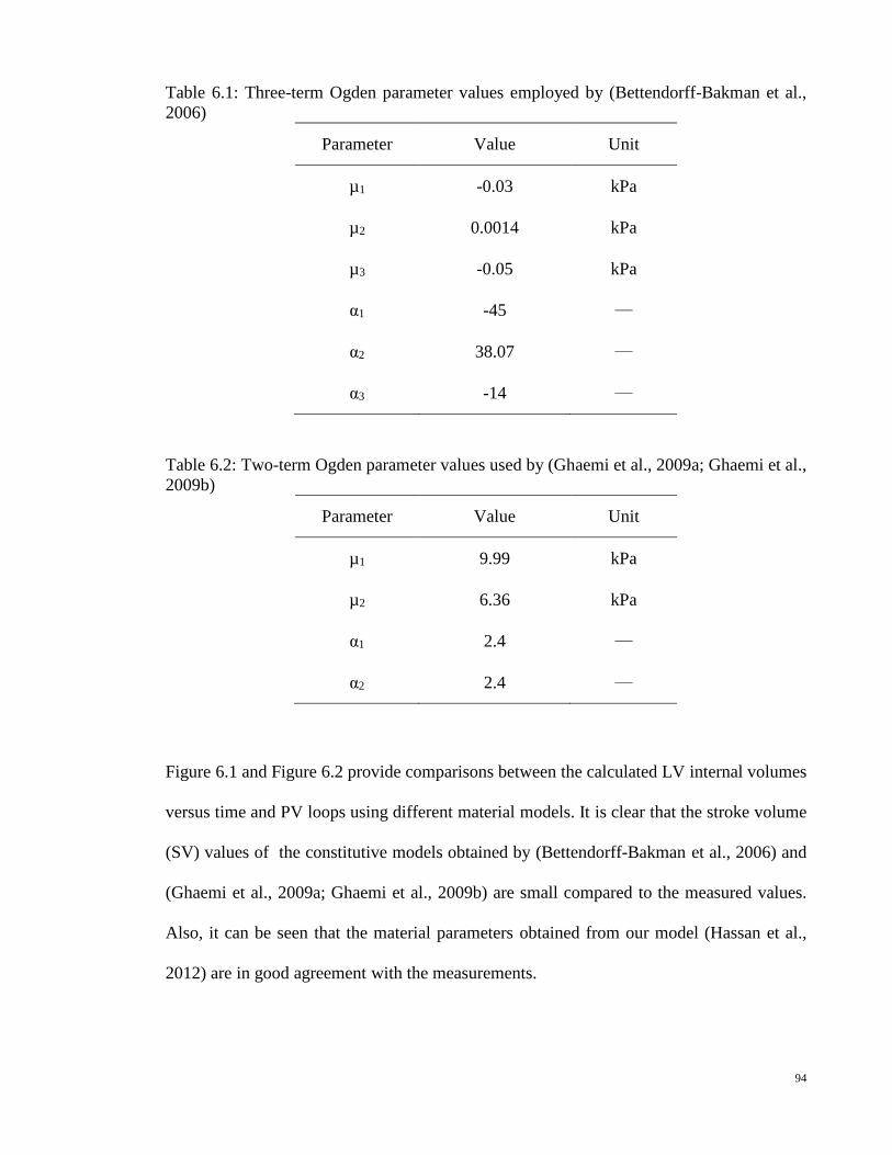
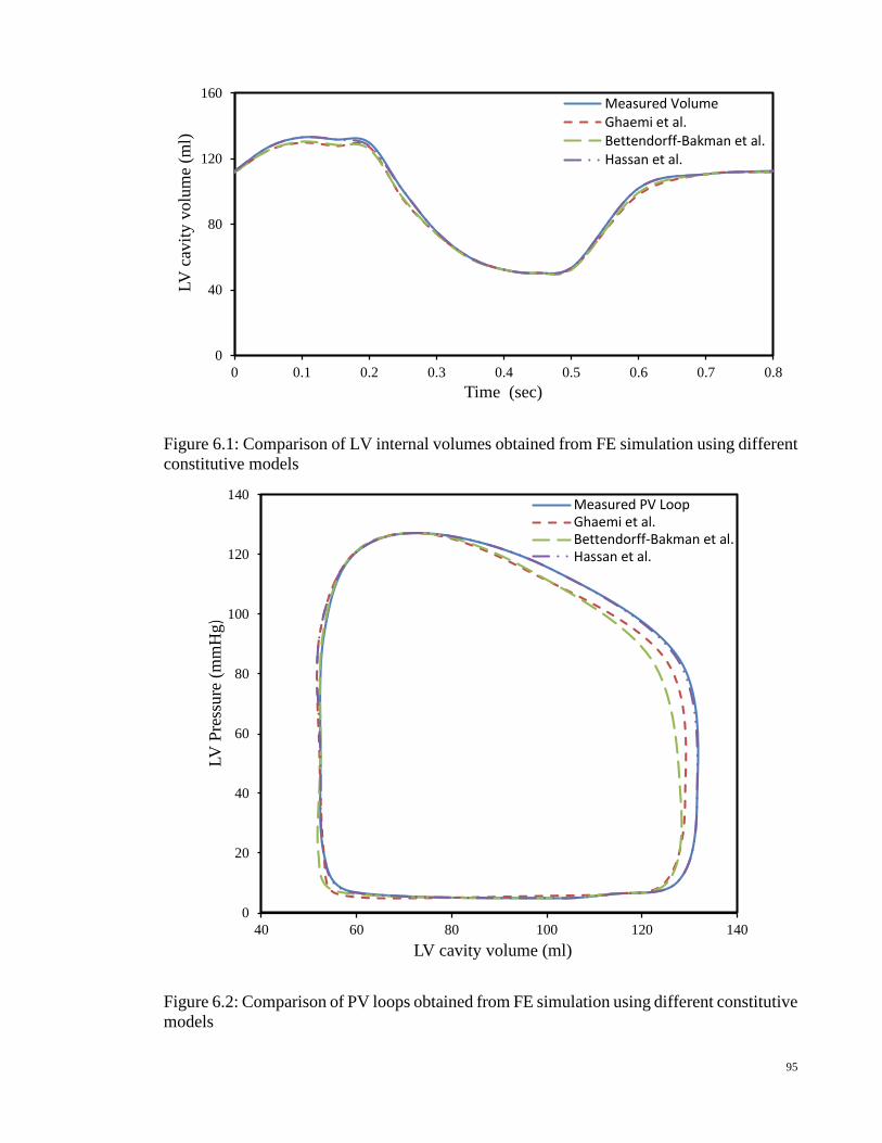
Figure 6.1 Comparison of LV internal volumes obtained from FE simulation using
different constitutive models
95
Figure 6.2 Comparison of PV loops obtained from FE simulation using different
constitutive models
95
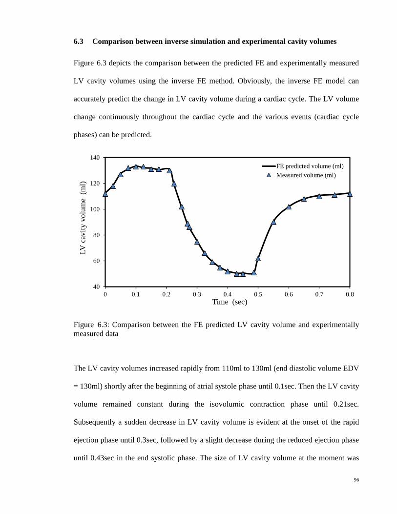
Figure 6.3 Comparison between the FE predicted LV cavity volume and
experimentally measured data
96
Figure 6.4 (a) Measured LV pressures vs. time for two different cardiac cycles; (b)
Measured LV cavity volumes vs. time; (c) FE computed myocardial
tissue bulk modulus vs. time
98
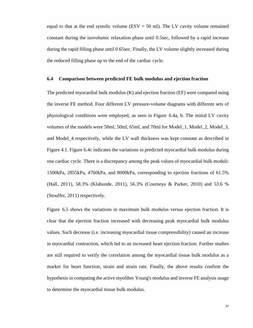
Figure 6.5 Comparison between the FE predicted maximum bulk modulus and
ejection fraction
99
xiii
LIST OF TABLES
Table 4.1 Values of two-term Ogden parameters found by (Hassan et al., 2012) 63
Table 4.2 Collagen material properties (Bagnoli et al., 2011) 63
Table 4.3 The corresponding fiber helix angle (β) variations through the eight
regions
67
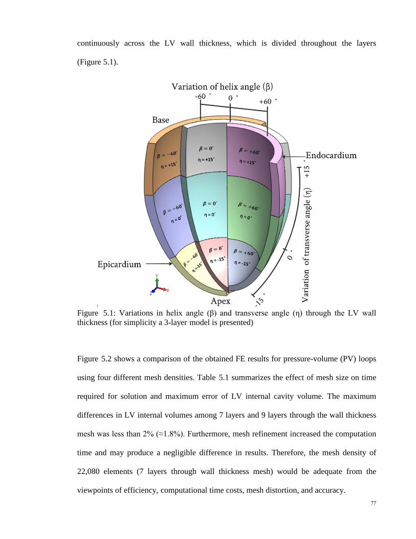
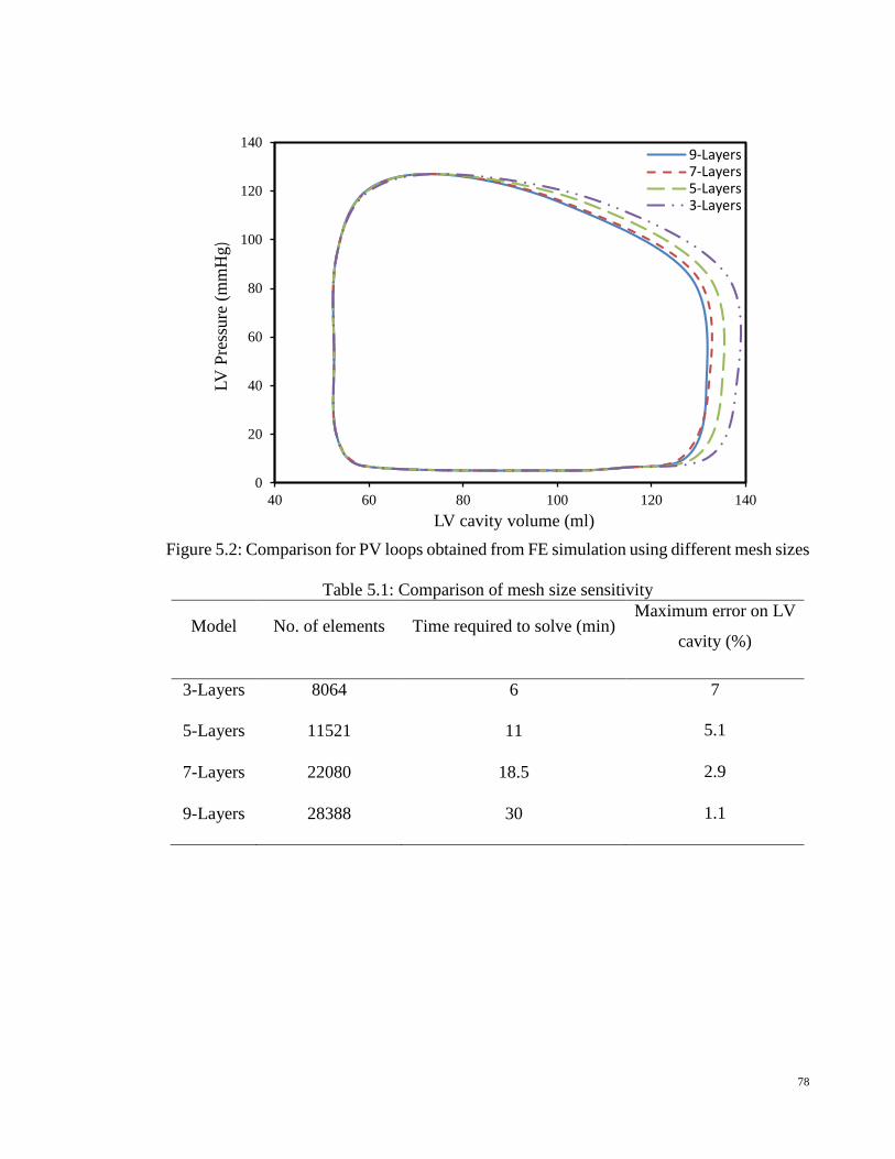
Table 5.1 Comparison of mesh size sensitivity 78
Table 6.1 Three-term Ogden parameter values employed by (Bettendorff-
Bakman et al., 2006)
94
Table 6.2 Two-term Ogden parameter values used by (Ghaemi et al., 2009a;
Ghaemi et al., 2009b)
94
xiv
LIST OF SYMBOLS AND ABBREVIATIONS
Symbols Description
𝑡𝑡 � Nominal traction force vector
𝜇𝜇𝑛𝑛, 𝛼𝛼𝑛𝑛 Material constants (Ogden parameters)
∆𝑢𝑢 Incremental displacement vector
∆𝜎𝜎 Incremental stress vector
∆𝜖𝜖 Incremental strain vector
B Strain-displacement relation matrix
b, {bi} External body force vector
C, {CMN} Right Cauchy-Green or Green deformation tensor
Ca2+ Calcium ion
Cij ij-th component of the right Cauchy-Green deformation tensor C
D Stress-strain relation matrix
dX Undeformed line segment
dx Deformed line segment
E Young’s modulus
Edef Deformation energy
Eexf Energy due to external forces
Eg Global energy functional
f, {f i} Acceleration vector
F, {FiM} Deformation gradient tensor
I Vector of resorting loads corresponding to element internal loads
i j Base vectors for the rectangular cartesian coordinate system
J Volumetric ratio
K Bulk modulus
k Global stiffness matrix
ke Element stiffness matrix
n Number of element in the left ventricle model
N Element shape function
Øtot Total myofiber volume fractions
xv
P Applied load vector
Pbp Force generated by blood pressure on the surface of the endocardium
Pma Active force generated by the myocardium muscles
Psp Force generated by pressure external from surrounding organs
S First Piola-Kirchhoff stress tensor or surface on V where �̃�𝑡 is applied
s, {si} External stress vector
sendo Surface area of elements on the endocardial surface
sepi Surface area of elements on the epicardial surface
t, {ti} Internal stress or traction vector
T, {TMN} Second Piola-Kirchhoff stress tensor
TOL Relative displacement tolerance
u, u0 Displacement vector in deformed and undeformed body, respectively
V Initial configuration of the material
v, {vi} Velocity vector
ve Volume of the element
W Strain energy function
Wact Active component of strain energy function
Wpass Passive component of strain energy function
α A large value corresponding to the bulk modulus
β Helix angle
δCij Variation of Cij due to δu
δu Variation of the displacement vector u
δui i-th component of δu
η Transverse angle
λ Lagrange multiplier
λ1, λ2, λ3 Principal stretch ratios
σi j Physical Cauchy stress components
Ψ A function to describe volume change
𝛎𝛎 Poisson’s ratio
𝛒𝛒, 𝛒𝛒0 Densities for deformed and undeformed configurations, respectively
xvi
Abbreviations Description
3D Three dimensions
ADP Adenosine diphosphate
ATP Adenosine triphosphate
AV Atrioventricular
CAD Coronary Artery Disease
DT Diffusion tensor
ECG Electrocardiography
EDV End diastolic volume
EF Ejection fraction
ESV End systolic volume
FE Finite element
LV Left ventricle
MI Myocardial infarction
MRI Magnetic Resonant Imaging
MRT Magnetic Resonant Tagging
P Phosphate
PV Pressure-Volume
SA Sinus-atrial
SV Stroke volume
WHO World Health Organization
xvii
INTRODUCTION
1.1 General background
Heart disease is the leading cause of death nearly in the entire world, especially in developed
countries. According to the World Health Organization (WHO), deaths caused by heart
disease each year are more than by cancer, diabetes, respiratory diseases, and accidents
combined. Death attributable to heart disease in the United States of America today is over
25% of the total number of deaths.
Computational cardiac models are undoubtedly powerful tools used to guide successful
patient therapy design. They not only play a crucial role in reproducing biological cardiac
behavior by incorporating experimental findings but also serve as a virtual testing
environment for predictive analyses where experimental techniques fall short.
1.2 Anatomy and functions of the heart
The heart is a hollow muscular organ located behind and to the left of the breastbone and
between the lungs (Toronto, 1964). The heart is contained within a sack called “the
pericardium,” which sits on top of the diaphragmatic muscle and is surrounded by the
ribcage. These structures all serve to protect the heart. As shown in Figure 1.1, the
pericardium consists of two parts, the inner serous pericardium and the outer fibrous
pericardium. (Iaizzo, 2009).
1
Figure 1.1: Internal anatomy of the heart. The walls of the heart consist of three layers – the superficial epicardium, the middle myocardium composed of cardiac muscle, and the inner endocardium (Iaizzo, 2009)
The heart has two separate pumps, the right and left side, which work together. The right
side of the heart collects de-oxygenated blood from the body via the superior and inferior
vena cava in the right atrium; the right atrium pumps the blood through the tricuspid valve
into the right ventricle; the right ventricle pumps the blood through the pulmonary valve into
the lungs -- a cycle known as “pulmonary circulation.” In the lungs, carbon dioxide is
removed from the blood and oxygen is picked up. Meanwhile, the left side of the heart
collects oxygenated blood from the lungs via the pulmonary veins in the left atrium; the left
atrium pumps the blood through the bicuspid valve into the left ventricle (LV); the LV pumps
the blood out of the heart through the aortic valve, a cycle called “systemic circulation.”
When this pumping cycle is complete, the aortic valve closes to prevent blood from dropping
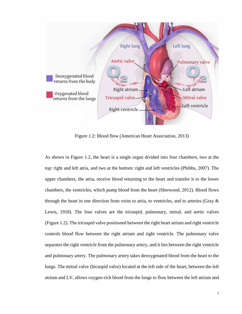
back into the heart (Figure 1.2) (Martini et al., 2012).
As shown in Figure 1.2, the heart is a single organ divided into four chambers, two at the
top: right and left atria, and two at the bottom: right and left ventricles (Phibbs, 2007). The
upper chambers, the atria, receive blood returning to the heart and transfer it to the lower
chambers, the ventricles, which pump blood from the heart (Sherwood, 2012). Blood flows
through the heart in one direction from veins to atria, to ventricles, and to arteries (Gray &
Lewis, 1918). The four valves are the tricuspid, pulmonary, mitral, and aortic valves
(Figure 1.2). The tricuspid valve positioned between the right heart atrium and right ventricle
controls blood flow between the right atrium and right ventricle. The pulmonary valve
separates the right ventricle from the pulmonary artery, and it lies between the right ventricle
and pulmonary artery. The pulmonary artery takes deoxygenated blood from the heart to the
lungs. The mitral valve (bicuspid valve) located at the left side of the heart, between the left
atrium and LV, allows oxygen-rich blood from the lungs to flow between the left atrium and
3
LV. The aortic valve separates the LV from the aorta and controls blood flow between the
LV and the main blood vessel leaving the heart (Snell, 2011).
The sinus-atrial (SA) node contains pacemaker cells, which help the heart beat in a regular
rhythm (Figure 1.3). The SA node’s activity, i.e., the heart rate, is essentially controlled by
three sources. First, the SA node has its own intrinsic rhythm (more than 60 beats per
minute). Second, the sympathetic as well as the parasympathetic nervous system are directly
coupled to the SA node and have an increasing or decreasing effect on the heart rhythm,
respectively. Third, a number of hormones, such as adrenalin, influence the SA node’s
activity (Gacek, 2012).
The SA node sends out a regular electrical impulse, causing the atria to contract and pump
blood into the bottom chambers, or ventricles. After the atria contract, the electrical impulse
reaches the ventricles through a junction box called the atrioventricular (AV) node, which is
located at the base of the right atrium. The AV node is only a conductive link between the
atria and ventricles. This node acts as a filter that permits the atrial contraction to fill the
ventricles with blood before the ventricles begin to contract. The bundle of His represents a
continuation of the AV node and provides the electrical connection to the ventricles. It
separates into two parts: one that activates the right ventricle and the other the LV. These
parts descend on either side of the septum and divide into hundreds of tiny nerve fibrils
called Purkinje fibers throughout the wall of each ventricle. Purkinje fibers are conductile
cells that conduct action potentials very rapidly. These fibers, however, cause the ventricles
to contract and pump out the blood. The blood from the right ventricle goes to the lungs and
the blood from the LV goes to the body (Berne & Levy, 1996; Smith & Roberts, 2011). This
process takes 0.8 seconds and is a single heartbeat. The electrical currents occurring during
depolarization (contraction) and repolarization (relaxation) of the myocytes are powerful
4
enough to be detected by electrodes on the surface of the body using conductive adhesive
patches. The obtained recording is called the electrocardiogram (ECG). By comparing the
information obtained from an ECG, a clinician can monitor the heart’s electrical activity,
which is directly related to the performance of specific nodal, conducting, and contractile
components (Davey et al., 2008).
Figure 1.3: Conduction system of the heart (American Heart Association, 2013)
The ECG is subdivided into two segments that are separated by three waves: the P wave
represents atrial contraction, the complex QRS represents LV depolarization, and the T wave
represents the ventricles’ repolarization (Figure 1.4).
5
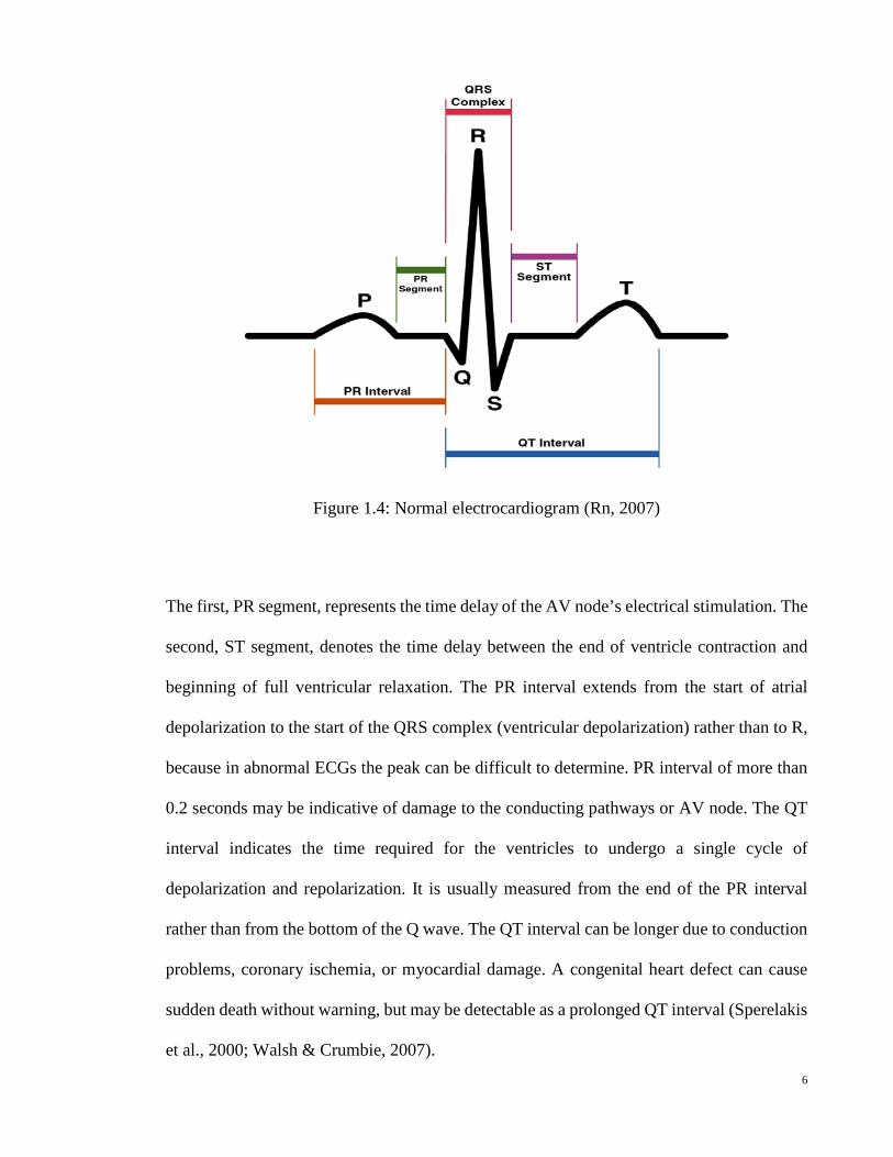
Figure 1.4: Normal electrocardiogram (Rn, 2007)
The first, PR segment, represents the time delay of the AV node’s electrical stimulation. The
second, ST segment, denotes the time delay between the end of ventricle contraction and
beginning of full ventricular relaxation. The PR interval extends from the start of atrial
depolarization to the start of the QRS complex (ventricular depolarization) rather than to R,
because in abnormal ECGs the peak can be difficult to determine. PR interval of more than
0.2 seconds may be indicative of damage to the conducting pathways or AV node. The QT
interval indicates the time required for the ventricles to undergo a single cycle of
depolarization and repolarization. It is usually measured from the end of the PR interval
rather than from the bottom of the Q wave. The QT interval can be longer due to conduction
problems, coronary ischemia, or myocardial damage. A congenital heart defect can cause
sudden death without warning, but may be detectable as a prolonged QT interval (Sperelakis
et al., 2000; Walsh & Crumbie, 2007). 6
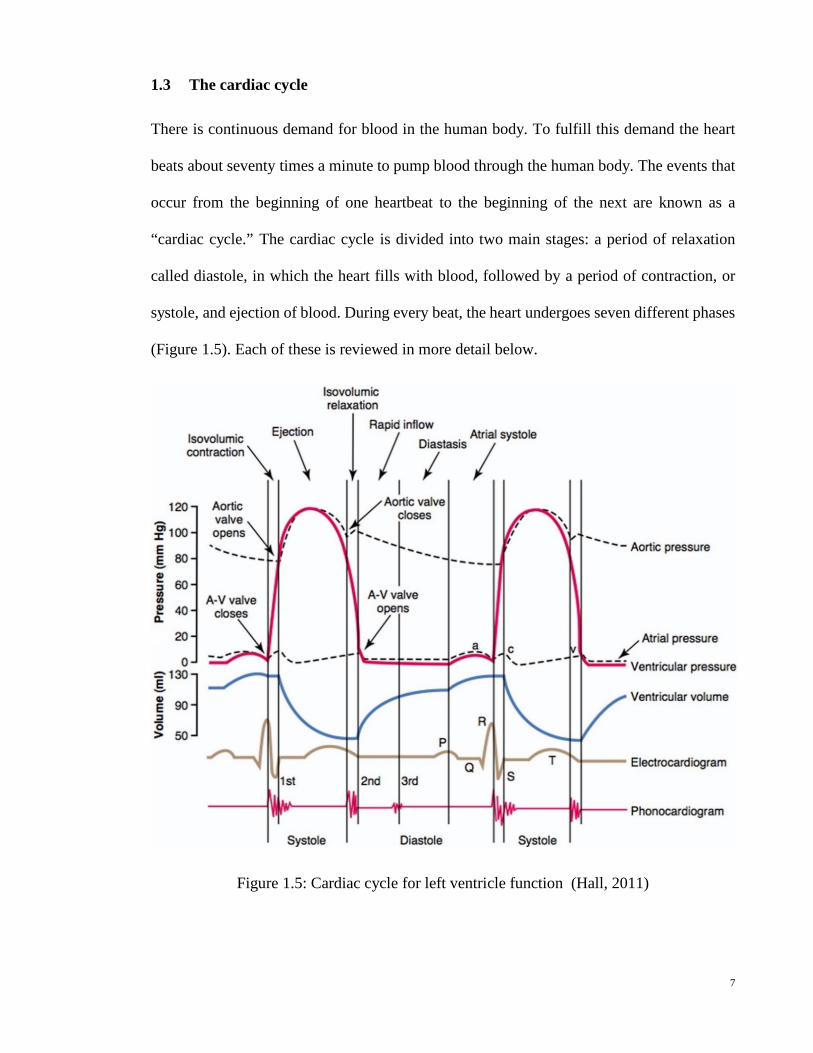
1.3 The cardiac cycle
There is continuous demand for blood in the human body. To fulfill this demand the heart
beats about seventy times a minute to pump blood through the human body. The events that
occur from the beginning of one heartbeat to the beginning of the next are known as a
“cardiac cycle.” The cardiac cycle is divided into two main stages: a period of relaxation
called diastole, in which the heart fills with blood, followed by a period of contraction, or
systole, and ejection of blood. During every beat, the heart undergoes seven different phases
(Figure 1.5). Each of these is reviewed in more detail below.
Figure 1.5: Cardiac cycle for left ventricle function (Hall, 2011)
7
Atrial Systole (Atrial Contraction) is the first phase of a cardiac cycle, which occurs when
the left atrium contracts causing an increase in left atrial pressure (Sandhar, 2004). Following
atrial contraction, the left atrial pressure eventually falls causing the mitral valve to close,
thus concluding the diastole phase (Klabunde, 2011).
Isovolumetric Contraction: This is when the valves of the left and right ventricles are
closed and the myocardium is contracting. The cavity pressure increases while the volume
stays constant (Sicar, 2008).
Rapid Ejection: As soon as the pressure in the left ventricle exceeds the pressure in the
aorta, the aortic valves open and blood flows rapidly from the ventricle into the aorta. This
corresponds to a sharp decrease in ventricular volume. Atrial pressure drops below venous
pressure, and the atria begin to fill at this time (Rhoades & Bell, 2009).
Reduced Ejection: Following rapid ejection, the rate of outflow from the ventricle decreases
and the ventricular and aortic pressures begin to decrease. At this point, muscle fibres have
become shorter and can no longer contract forcefully. The venous pressure is still greater
than atrial pressure, and the atria are still filling (Deepa, 2012).
Isovolumetric Relaxation: During the isovolumetric relaxation phase the myocardium is
relaxing and all valves are closed, so the pressure and tension drops very rapidly as the
volume of the ventricles does not change; the residual volume of blood in the LV is
approximately 40-50 ml (Cosin Aguilar et al., 2009).
Rapid Filling Phase (Rapid Inflow): In the rapid filling phase, ventricular pressure
decreases below atrial, the atrioventricular valves open and filling occurs rapidly from 50 to
85 ml (Sherwood, 2012).
8
Reduced Filling Phase (Diastasis): It is the longest phase of the cardiac cycle in which the
left ventricle continues to fill with blood and expands slowly until nearly full (Sembulingam
& Sembulingam, 2002). The typical amount of blood in the LV after filling is approximately
110-120 ml. As the ventricle fills, the intraventricular pressure increases, slowing the filling
rate (Levy et al., 2007).
1.4 Myocardium contraction
The myocardium consists of muscle fibers held together by collagen fibers (Figure 1.6). The
muscle fibers, or myocytes, make up approximately 70% of the myocardial volume. The
network of collagen fibers accounts for only about 1.5% of the myocardium (LeGrice et al.,
1995; Stevens & Hunter, 2003; Aaronson et al., 2012).
The muscle fiber actually consists of a bundle of several hundred smaller fibers called
myofibrils. As seen in Figure 1.7, the muscle fibers themselves make up larger units called
fascicles. Numerous fascicles, in turn, are bound together by fascia to form a section of
muscle. There are approximately one hundred fibers in a fascicle, and each muscle fiber
contains between one thousand and two thousand myofibrils. When viewed under an
electron microscope, it is visible that each myofibril is primarily composed of two kinds of
filaments (thick and thin) organized into regular, repeating sub-units. These sub-units are
called sarcomeres (the function units of contraction) (Davies et al., 2004).
9
Figure 1.6: Schematic of fibrous sheet structure of cardiac tissue. The myocardium is composed of muscle fibers bound together by a mesh of collagen fibers
Figure 1.7: Step dissection of muscle tissue, showing a sample muscle section, fascicle, muscle fiber, myofibril, and sarcomere (Davies et al., 2004)
10
Thick filaments are made of hundreds of molecules of the protein myosin. At the molecular
level, a thick filament is a shaft of myosin molecules arranged in a cylinder. Thin filaments
are approximately half the diameter of thick filaments, and primarily contain the
protein actin. The thin filaments look like two strands of pearls twisted around each other
(Figure 1.8 and 1.9).
Figure 1.8: Real sarcomere (Sherwood, 2012)
Figure 1.9: The sarcomere -- the contractile mechanism of muscle (Koeppen & Stanton, 2009)
11
In order for the muscle to contract, the thick and thin filaments must slide past each other,
moving Z disks from either end of the sarcomere closer to each other. During this shortening
of sarcomeres, there is no change in the length of either thick or thin filaments (Figure 1.8
and Figure 1.9). This is the sliding-filament mechanism of muscle contraction. A sarcomere
shortens when myosin heads and thick filaments form a cross-bridge with actin molecules
and thin filament. Cross-bridge formation is initiated when calcium ions released from the
sarcoplasmic reticulum bind to troponin. This binding causes troponin to change shape
(Figure 1.10). Tropomyosin moves away from the myosin binding sites on actin allowing
the myosin head to bind to actin and form a cross-bridge. Also note that the myosin head
must be activated before the cross-bridge cycle can begin. This occurs when adenosine
triphosphate (ATP) binds to the myosin head and is hydrolyzed to adenosine diphosphate
(ADP) and inorganic phosphate (P). The energy liberated from the hydrolysis of ATP
activates the myosin head, forcing it into a cocked position (Clark, 2005; Plowman & Smith,
2013)
Figure 1.10: Troponin changes shape and pulls tropomyosin out of the myosin head binging sites (Widmaier, 2013)
Cross-bridge cycle may be divided into four steps (Figure 1.11):
1. Cross-bridge formation 2. The power stroke
3. Cross-bridge detachment 4. Reactivation of myosin head
12
Figure 1.11: The cross-bridge cycle: how muscle fibers contract (Widmaier, 2013)
The first step in the cross-bridge cycle is the binding of the activated myosin head with actin,
and releasing inorganic phosphate (P) to form a cross-bridge. The second step is the power
stroke. In this phase, ATP is released and the activated myosin head pivots, sliding the thin
filament toward the center of the sarcomere. The third step entails the dissociation of myosin
and actin. When another ATP binds to the myosin head, the link between the myosin head
and actin weakens and the myosin head detaches. The fourth step is the activation of the
myosin head. During this step, ATP is hydrolyzed to ADP and inorganic phosphate (P). The
energy released during hydrolysis reactivates the myosin head returning it to the cocked
position (Chandler & Brown, 2008; Katz, 2011).
As long as the binding sites on actin remain exposed, the cross-bridge cycle will repeat; as
the cycle repeats the thin filaments are pulled toward each other and the sarcomere shortens.
This shortening causes the whole cardiac muscle to contract. The cross-bridge cycle ends
when calcium ions are actively transported back into the sarcoplasmic reticulum. Troponin
13
returns to its original shape allowing tropomyosin to glide over and cover the myosin binding
sites on actin (Sherwood, 2012).
1.5 Heart diseases
Heart disease is a broad term used to describe a wide range of diseases affecting the heart.
Most people think there is only one reason for heart disease but in fact, there are several
causes potentially affecting the function of the heart, with over 50 different types of heart
disease. Some of the more common heart diseases are described below:
Coronary Artery Disease (CAD): CAD is the leading cause of mortality in the United
States, accounting for more than 250,000 deaths annually (Bogaert et al., 2005; Rao &
Thanikachalam, 2005). CAD occurs due to the narrowing of the coronary artery that supplies
blood and oxygen to the heart muscle. As we get older, the lining of the heart artery gets
damaged and thickened due to the accumulation of "plaque," which is a combination of fatty
material, cholesterol, and other substances. This slow process is known as "Atherosclerosis"
and can sometimes cause cracks or fissures in the coronary artery. Consequently, the blood
cells called "Platelets" stack onto the damaged area and start the formation of blood clots
that prevent blood flow to the heart muscle, which is necessary for survival (Figure 1.12). In
an effort to compensate for the final functional myocytes, left ventricle remodeling may
occur where the heart enlarges and expands along with increased thinning of the heart wall,
causing adverse geometric and functional changes; if left untreated, this may lead to heart
Figure 1.12: Progression of heart attack. (a) Plaque buildup in the walls of the coronary artery; (b) Plaque becomes unstable and ruptures; (c) Platelets stack on the damaged area and start forming blood clots; (d) Clot completely blocks the coronary artery resulting in the death of all muscle tissue below the blockage (American Heart Association, 2013)
Myocardial infarction (MI) and Ischemia: MI often entails myocardial cell death owing
to a number of reasons. Most commonly, myocardial infarction occurs when normal blood
flow to the heart decreases (Figure 1.12). Reduced blood flow usually results from a
thrombus in the coronary artery (Gaasch et al., 1985; Anversa & Sonnenblick, 1990; Yusuf
et al., 2004).
Hypertrophy (Hypertrophic Cardiomyopathy): This is when the chamber muscle tissue
enlarges due to one of several different causes (Figure 1.13). The most common cause is
high blood pressure, something that requires the heart muscle to work harder. As the
workload increases, the chamber walls grow thicker, lose elasticity and may eventually fail
to pump with as much force as that of a healthy heart (Alpert, 1971; Katholi & Couri, 2011).
Dilated (Congestive) Cardiomyopathy: A weakness in the heart walls causes them to
enlarge (Figure 1.13). In some cases, it prevents the heart from relaxing and filling with
blood as it should. Over time, it can affect the whole heart (Fuster et al., 1981; Wheeler et
al., 2009).
15
Figure 1.13: Illustration of the differences between a normal heart, hypertrophic cardiomyopathy, dilated cardiomyopathy, and with electrical disorders (arrhythmogenic right ventricular cardiomyopathy) (American Heart Association, 2013)
16
Electrical disorders: Include abnormal heart impulse rhythm and can be caused by
problems with the heart’s electrical system (Figure 1.13). The electrical impulses may
happen too fast, too slowly, or erratically (tachycardia, bradycardia and arrhythmia) causing
the heart to beat too fast, too slowly, or erratically (Farwell & Gollob, 2007).
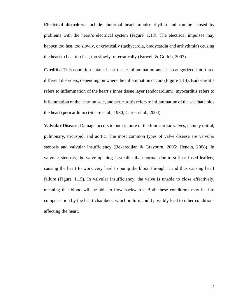
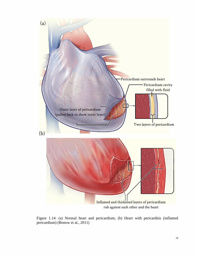
Carditis: This condition entails heart tissue inflammation and it is categorized into three
different disorders, depending on where the inflammation occurs (Figure 1.14). Endocarditis
refers to inflammation of the heart’s inner tissue layer (endocardium), myocarditis refers to
inflammation of the heart muscle, and pericarditis refers to inflammation of the sac that holds
the heart (pericardium) (Steere et al., 1980; Carter et al., 2004).
Valvular Disease: Damage occurs to one or more of the four cardiac valves, namely mitral,
pulmonary, tricuspid, and aortic. The most common types of valve disease are valvular
stenosis and valvular insufficiency (Bekeredjian & Grayburn, 2005; Henein, 2008). In
valvular stenosis, the valve opening is smaller than normal due to stiff or fused leaflets,
causing the heart to work very hard to pump the blood through it and thus causing heart
failure (Figure 1.15). In valvular insufficiency, the valve is unable to close effectively,
meaning that blood will be able to flow backwards. Both these conditions may lead to
compensation by the heart chambers, which in turn could possibly lead to other conditions
affecting the heart.
17
Figure 1.14: (a) Normal heart and pericardium; (b) Heart with pericarditis (inflamed pericardium) (Bonow et al., 2011)
18
Figure 1.15: Aortic valve in normal and stenosis states (Otto & Bonow, 2013)
1.6 Myocardium bulk modulus
One of the tools with the potential to facilitate the early detection of human heart failure is
to understand the mechanical behavior of the LV in normal and diseased states. Then there
would be continuous interest in determining the material properties of the myocardium by
mechanically testing excised strips from it. These strips, under prescribed homogeneous
loading conditions, produce stress-strain relationships. These tests were originally done
uniaxially, but more recently, biaxial tests have also been performed. A uniaxial test is used
to define passive stress-strain relationships in the fiber’s direction (Kohl et al., 2011). It is a
very useful test in determining the general characteristics of the behavior of cardiac tissue in 19
both healthy and diseased states, but is not sufficient to provide a unique description of the
myocardium’s three-dimensional (3D) constitutive behavior. Due to the incompressibility of
cardiac tissue, biaxial tests can be used to determine certain multidimensional stress-strain
relationships for the fibers and cross-fibers (Fung & Cowin, 1994). Despite the frequent
assumption that human myocardial tissue is incompressible, the fact remains that all
myocardial tissue has some degree of compressibility. Furthermore, the subject on the
compressibility of myocardium tissue is raised as a result of systolic intra- and extra-vascular
blood displacements (Yin et al., 1996). Consequently, it is evident that myocardium tissue
compressibility changes during the cardiac cycle.
The information embodied in the myocardial tissue bulk modulus adds further insight to the
mechanical nature of the soft tissue. Bulk modulus is very important as a standalone
parameter and as additional information to shear/Young's modulus. Precise myocardial bulk
modulus values are especially required to improve the accuracy of finite element (FE)
simulation for human heart modeling. In the last several decades, publications related to
cardiac modeling have addressed the myocardial bulk modulus from many different
perspectives. The published myocardial bulk modulus values recorded by researchers who
were interested in simulating LV performance during the diastolic phase are quite small, for
instance 28kPa (Bettendorff-Bakman et al., 2006) and 160kPa (Veress et al., 2005). This
may be attributed to small changes in ventricular wall volume. Some studies evaluated the
bulk modulus under the assumption that during the rapid filling phase, the volume change
of the ventricular wall should be less than 10%. Additionally, relatively high bulk modulus
values were used by researchers who analyzed the systolic phase, e.g., 380kPa (Shim et al.,
2012), 600kPa (Dorri et al., 2006), and 25MPa (Marchesseau et al., 2012). High values for
the bulk modulus during the systolic phase are due to the systolic intra- and extra-vascular
20
blood displacements that give rise to tissue compressibility. A mean, constant value for
myocardial bulk modulus was assumed during each cardiac phase.
Despite the widespread use of uniaxial and biaxial tests for determining myocardial
characteristics, there are four major problems that arise from these kinds of studies (Yettram
& Beecham, 1998; Périé et al., 2013):
1. Tests were carried out on non-human tissue, and as a result may not be directly
applicable to humans.
2. The properties may not be directly relevant to FE heart models due to the
myocardium’s heterogeneous behavior.
3. The myocardium’s mechanical properties change drastically immediately after
death.
4. There is variation in the mechanical property values according to experimental
loading conditions.
All the above limitations prompt researchers to find alternate ways of running experiments,
without having to excise samples from the myocardium. Hence, a group of researchers have
moved toward using MRI and FE or mathematical methods to determine mechanical
properties in vivo (Augenstein et al., 2006; Wang et al., 2009). Others have applied scanning
acoustic microscopy with high frequency ultrasound to measure the bulk modulus and
describe the mechanical properties of the myocardium (Dent et al., 2000). However, most
bulk modulus experimental values obtained from these studies are very high (≈ 3GPa) and
cannot be used directly in FE modeling.
21
1.7 Problem statement
With heart disease being such a major health problem as well as a large financial strain on
healthcare, it is no wonder that over recent years, cardiology has featured prominently as a
medical research field. It is in the hopes of better understanding the functions of the heart
and the effect diseases have, that research has continued. Greater knowledge may enable
earlier disease detection and medical intervention at less advanced stages. Research may also
pave the way towards more effective treatment.
The heart is extremely complicated in terms of its structure and function. It would be a grave
mistake to model it purely from a mechanical point of view without an appreciation of its
complex biological nature. Therefore, this research has aimed to model the behavior of the
human heart muscle including an accurate description of both muscle fiber orientation and
material properties.
For many years, researchers have attempted to determine the material properties of
myocardium involving precise measurement of the ventricles of animals. Only a few have
used data gathered from human subjects, since this data is usually hard to come by and is
often severely limited in terms of quality and quantity. The research introduced a novel
method to determine the material properties of beating human heart, and in particular the
myocardial bulk modulus.
1.8 Study objectives
The first main objective of this research is to develop a 3D model of the LV, which is the
main pumping chamber and most common site for heart disease, based on an accurate
description of both muscle fiber orientation and material characteristics. The proposed model
is used to study the effects of myocardial fiber architecture on LV mechanics.
22
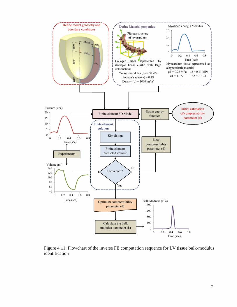
The second objective, and to overcome the above shortcomings in determining live tissue
properties, an inverse FE procedure using the ANSYS® computer code approach is suggested
to determine, in vivo, the myocardial tissue bulk modulus during the cardiac cycle. The
proposed inverse technique is based on published, experimentally measured LV pressure-
volume curves. By using published LV experimental data as output, the bulk modulus versus
time curve is traced with an inverse technique. The recurring changes of myocardial tissue
bulk modulus in the LV wall during a cardiac cycle result in a highly efficient global function
of the normal heart. Therefore, the myocardial bulk modulus can be effectively used as a
diagnostic tool of heart ejection fraction.
1.9 Thesis outline
The first chapter of this dissertation concerns the physiology and architecture of the heart.
Basic concepts of the heart’s anatomy and functions are initially presented. Then the cardiac
cycle, myocardial contraction process, and heart diseases are outlined.
In order to understand the evolution of the ventricle mechanics model developed in the
dissertation, a brief history of cardiac modeling research is presented in chapter two.
Ventricle model development has ranged from thin walled to thick walled and FE models.
Moreover, the mechanical behavior of cardiac tissue is modeled using a variety of material
response functions, from a simple phenomenological description to a biophysical
representation based on the microscopic myocardial architecture. Following some historical
remarks, the aim of the present work and study plan are presented.
In chapter three, the heart tissue is studied from a continuum mechanics point of view.
Selected elements of continuum mechanics are outlined. The approach for LV motion
formulation and material behavior of the myocardium tissue are discussed.
23
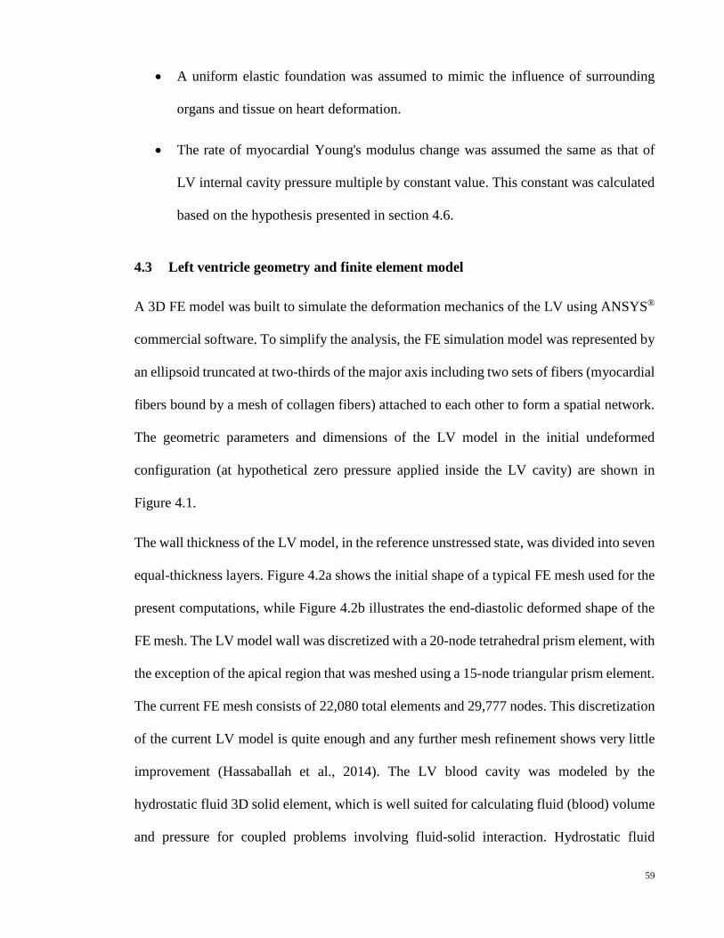
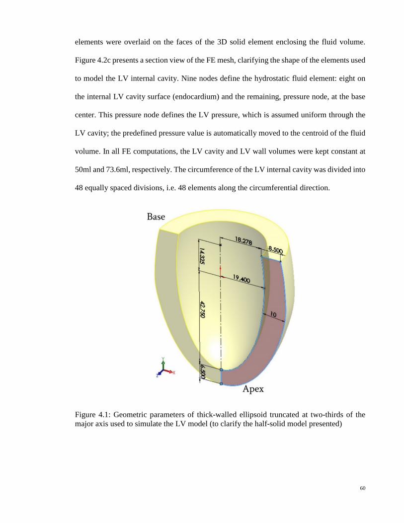
The implementation of an FE model of the LV is shown in chapter four. To this end, a thick-
walled ellipsoid truncated at two-thirds of the major axis is chosen for modeling a human
LV. Appropriate boundary conditions are also imposed, and the constitutive behavior
including detailed information about fiber orientation patterns is prescribed. A new approach
using a direct FE method of studying the effect of myocardial fiber architecture on LV
mechanics is presented. Moreover, a novel approach using the inverse FE method to
determine, in vivo, the myocardial bulk modulus during a cardiac cycle is introduced. This
chapter plays a central role in the dissertation; however, since the procedures are based on a
simplified geometry, there is still margin for improvement with respect to accuracy and
completeness of fiber orientation and material properties. At the end of this chapter, the
merits and limitation of the proposed FE model are discussed.
The results of FE implementation are discussed in chapter five. In particular, the sensitivity
of LV mechanics, such as mesh density, myofiber volume fraction, myofiber orientation,
and different constitutive models is presented using the direct FE method. Besides,
determining the human myocardial bulk modulus and the correlation between LV
repolarization and myocardium tissue compressibility are described using the inverse FE
method. A balanced discussion taking into account work from other groups is provided in
chapter six.
Finally, based on the results and discussion presented in chapters five and six, the
conclusions and recommendations are drawn in chapter seven.
24
REVIEW OF CARDIAC MODELING RESEARCH
2.1 Introduction
The heart has always been recognized as the most important organ in the body. Even at the
beginnings of human civilization, the heart was considered by many cultures to contain
magical powers and often symbolized life itself. It is therefore hardly surprising that there
has been a great deal of interest in its structure and function. Even with all the technological
advances from different aspects, it remains impossible to understand the heart completely.
This is not due to a lack of quality research but owing to the complexity of the heart.
Simplified models can be useful to aid comprehend the behavior of the heart, to identify the
symptoms of heart failure and be able to study quantities that cannot be measured clinically
or in experimental settings, such as mechanical stress through the heart wall.
Cardiac research started in the days of early anatomists. In the 15th century, Leonardo Da
Vinci, whose Mona Lisa painting is the most famous in the world, described the movement
of the heart wall by using metal pins implanted through an animal’s chest wall (Keele, 1951).
This was an early attempt at describing and understanding the heart’s movement, in a limited
way. Now with advancements in instruments, heart muscle properties can be precisely
measured to provide the necessary information and comprehend the heart’s behavior.
2.2 The development of thin walled models
(Woods, 1892) made the first attempt to create a mathematical model of the LV using
Laplace’s law for the evolution of wall tension in the heart. This model approximates
myocardial tension to be proportional to the product of pressure and radius. Sixty years later
by (Burch et al., 1952), who employed a spherical model to study the effects of various
pressures and ventricular volumes on ventricle performance, as well as the effects of the
25
structural arrangement of muscular fibers and manner of contraction. Five years later
(Burton, 1957) demonstrated via Laplace’s law the importance of ventricle size and shape
on its performance. Assuming an ellipsoidal geometry, this type of analysis was refined by
(Sandler & Dodge, 1963), who investigated the role of ventricular pressure, volume and
shape in determining stress and tension within the LV wall during the cardiac cycle. These
forces were calculated by using Laplace’s law LV dimensions, as determined from biplane
angiocardiograms in human subjects with heart disease. A number of other authors utilized
this model to analyze human and animal patient data. (Wong & Rautaharju, 1968) and
(Ghista & Sandler, 1969) developed thick shell theories. Their analyses yielded nonlinear
stress distributions through the wall thickness, but it was not possible for Laplace’s law to
predict results. However, their assumptions with regard to the LV’s deformation behavior
are restricted. In addition, in the development of Laplace’s law their theories neglected the
effect of transverse normal stress (radial stress) and transverse shear deformation, which are
significant for the LV. (Mirsky, 1969) presented a system of different equations for the stress
equilibrium in the LV wall assuming an ellipsoidal geometry. His analysis of the stresses in
the ventricular wall indicates that maximum stresses occur at the inner layers and decrease
to a minimum at the epicardial surface -- a result partially validated experimentally.
2.3 The development of thick walled models
(Wong & Rautaharju, 1968) developed a formula that allows stress distribution calculations
for either a spherical thick shell, or an ellipsoidal shell, or a paraboloid of revolution. Their
analyses overcame the shortcomings of Laplace’s formula for a thin wall, which is an ill-
defined and practically meaningless quantity in a structure like the human LV. The formula
can be used for any of three configurations by varying certain parameters according to known
26
or assumed heart dimensions. This model is similar to that previously used by (Sandler &
Dodge, 1963), except that the stresses are allowed to vary through the wall’s thickness.
Despite inclusion in earlier models, bending and shear were still mostly not included.
(Streeter et al., 1970) proposed an analysis of stress in the LV wall based on the realistic
assumption that the myocardium is essentially composed of fiber elements that carry only
axial tension and vary in orientation through the wall. The geometry based on that obtained
from ten dogs rapidly fixed in situ at the end of diastole and end of systole.
(Ghista & Sandler, 1970) developed a simple model to predict the oxygen consumption rate
of a healthy LV. The geometry of this model was obtained by cineangiocardiography and
the LV chamber pressure was obtained by means of fluid-filled catheters subsequent to
retrograde or transeptal catheterization.
(Wong, 1973) produced a thick-walled ellipsoidal shell with non-uniform wall thickness LV
model. This model served to compute the sarcomere lengths at various wall layers during
the diastole. This method gives passive and active fiber tension as separate quantities within
each fiber and is used to analyze isovolumetric contraction, which assumes the myocardium
is homogenous, isotropic and viscoelastic. The fiber orientations obtained from (Streeter Jr
et al., 1969) and myocardium were modeled using Hill’s model and Huxley’s sliding
filament theory (Hill, 1938; Haselgrove & Huxley, 1973).
(Tözeren, 1983) came up with a cylindrical model of LV to estimate the local stresses and
deformations that occur during the cardiac cycle. The LV presented as thick hollow tube
composed of solid fibers embedded in an inviscid fluid matrix. It was concluded that wall
thickness and fiber orientation distribution hardly affect the pressure-volume relation in the
27
diastole. In the systole, the pumping efficiency was shown to increase with increasing
thickness of the modeled LV and with increasing contractility of the heart muscle fibers.
(Phillips & Petrofsky, 1984) calculated the active systolic elastic moduli for the
circumferential and longitudinal LV axes by using contractile filament stress and fiber strain.
Compressive strains were introduced into the model, which generated the fiber stresses.
These stresses and strains then helped calculate the active systolic elastic moduli for the
circumferential and longitudinal LV axes. These material property parameters were
determined at four points during cardiac systole. The data obtained from thirty-nine patients
with various pathological conditions was evaluated using pressure and volume data acquired
from single-plane cineangiography. The results indicate that the active moduli exponentially
decrease during cardiac systole.
(Kim et al., 1985) developed a mathematical method of estimating the local epicardial
deformation, wall thickness, and regional circumferential and longitudinal wall stress using
biplane coronary cineangiography for four dogs and a normal patient. In this method, the
motion images of the coronary artery bifurcation points were the local markers and the
accuracy of using these was compared with the more invasive method of using implanted
lead beads. The estimation results validate this analysis compared to the experimental results
based on the implanted lead beads. The main advantages of this method are that it can
evaluate the wall stress and wall deformation together with blood vessel conditions and it is
far safer than implanting lead beads.
2.4 The development of finite element models
(Janz & Grimm, 1972) were the first group of researchers who attempted to create an FE
model to analyze the mechanical behavior of a rat heart LV. The ventricle was modeled as a
28
heterogeneous, linearly elastic, thick-walled solid of revolution. The geometric data applied
was obtained from heart cross-sections of adult Sprague-Dawley albino male rats.
(Hamid & Ghista, 1974) developed an FE model of the LV to predict the stresses through
the wall chamber and aortic valve. The element type utilized in this model was developed
by (Zienkiewicz, 1971). The 20-noded isoparametric brick element is ideally suited for LV
modeling. The model geometry was obtained by cineangiocardiographic imaging at mid-
ejection.
(Nikravesh et al., 1981) developed a new FE model that obtains much better reconstructions
than offered by single or even bi-plane cineangiography. Besides, this method adds wall
thickness, something partially lacking in cineangiography. However, FE reconstructions
indicate that no analysis was performed on the FE meshes obtained.
(Yettram et al., 1983) presented an FE model to study the effect of myocardial fiber
architecture on the behavior of the human LV during diastole. The myocardium has a
complex anisotropic fiber structure. Variations were made to both fiber orientation and the
ratio of elastic moduli along and across the fibers. The results signify that at least in diastole,
when the LV is considered to be a passive structure under the action of internal blood
pressure, the effect of the real fiber arrangement is generally a reduction of deformation as
well as direct stresses. In spite of fiber angle changes across the wall, the analyses correctly
predicted the lack of LV rotation about the long axis.
(Horowitz et al., 1986) introduced an FE technique for simulating an entire cardiac cycle.
Time-sequential canine heart data obtained by dynamic computerized tomography served to
initiate the simulation as well as to provide real data for result evaluation. The model had
two element types: the “Truss” element to simulate the anisotropic nature of the myocardium
29
with varying fiber angles, and a basic 20-noded isoparametric brick element to form the basic
structure. The simulation allowed for the evaluation of time-varying stress and strain
distributions in the ventricle wall and active forces prevailing in the myocardial fibers.
(McPherson et al., 1987) developed a type of LV geometry FE analysis using 3D
echocardiographic reconstructions to study the effect of acute myocardial ischemia on the
myocardial elastic modulus. The data was collected from six open-chest dogs before and
after coronary occlusion using the data acquisition and reconstruction method proposed by
(Nikravesh et al., 1981). In the FE analysis after coronary occlusion, two analyses were
performed: one utilizing the control elastic modulus for all LV segments and one in which
ischemic (dyskinetic) segments were assigned a higher elastic modulus. It was concluded
that the myocardial diastolic elastic modulus was increased by ischemia and this approach
may facilitate the clinical assessment of intrinsic muscle stiffness.
(Bovendeerd et al., 1991) proposed another FE model of the LV based on the same geometric
data as (Huyghe et al., 1991). This model was meant to study the mechanics of the ischemic
LV during the cardiac cycle. The muscle fiber stiffness was assumed twice that in the fiber
direction than in the cross-fiber direction. The results show that global deformation was
asymmetric with respect to the ischemic region. It was deduced that the ischemic LV
pressure was about 12% lower, the ejection volume was 20% lower and aortic flow reduced
compared to a simulation without ischemic LV pressure.
(Fann et al., 1991) evaluated 2D subepicardial and subendocardial deformations in the LV’s
anterior, lateral, and posterior regions in a closed-chest, conscious dog heart. Eight dogs
underwent the placement of 22 radiopaque markers into in the LV myocardium. These were
located at the anterior, lateral and posterior subepicardial and subendocardial, mid-ventricle
level. Eight hours later, biplane videofluoroscopy was performed. It appeared that
30
circumferential shortening occurred in all layers and regions; similarly, longitudinal
shortening occurred in all layers except that of the posterior endocardium.
(Bovendeerd et al., 1992) investigated the dependence of local LV wall mechanics on
myocardial muscle fiber orientation using an FE model described by (Huyghe et al., 1991).
They considered an anisotropic model with the active and passive components of myocardial
tissue, dependence of active stress on time, strain and strain rate, activation sequence of the
LV wall and aortic afterload. The muscle fiber angle distribution through the myocardium
varied in order to make the active muscle stress homogeneous throughout the myocardium
layers. The muscle fiber angle is defined as the angle between the muscle fiber direction
and local circumferential direction, otherwise known as the helix angle. The transmural
variation of the helix angle assumed was from +60˚ at the endocardium through to 0˚ in the
mid-wall layers to -60˚ at the epicardium. The active muscle fiber stresses at the equatorial
region were 110 kPa, 30 kPa and 40 kPa in the respective myocardium layers from the
endocardium to the epicardium. It was concluded that the distribution of active muscle fiber
stress and muscle fiber strain across the LV wall is very sensitive to transmural distribution
of the helix fiber angle. However, the problem with this approach is that no consideration is
give to the effect that geometry may play on stress distribution. The LV is never stress-free,
so there are stress changes and no absolute stresses are implied.
(Hashima et al., 1993) developed a new means of studying the non-uniform mechanical
function that occurs in normal and ischemic ventricle myocardium. An array of 25 lead
markers was sewn onto the epicardium of the LV’s anterior free wall in an open-chest,
anesthetized canine preparation. Bi-plane cineangiography was used to track the position of
the markers before and during induced ischaemia. The strains during the cardiac cycle were
31
calculated using marker triplets. Large stain gradients were observed across the infarct
regions.
Subsequently, (Bovendeerd et al., 1994) investigated the influence of fiber direction
variations on the distribution of stress and strain in the LV wall using an FE model described
by (Huyghe et al., 1991) to simulate LV mechanics. An additional angle to helix fiber angle,
the transverse fiber angle, was employed to model the continuous course of the muscle fibers
between the inner and outer layers of the ventricle wall. This angle is defined as the angle
between the circumferential direction and fiber path projection onto the plane perpendicular
to the local longitudinal direction, whereas the helix fiber angle is defined as the angle
between the local circumferential direction and fiber path projection onto the plane
perpendicular to the local radial direction. Three model runs were carried out: the first run
had the transverse fiber angle always at zero and the helix fiber angle at -60º at the
epicardium, 0º at the mid-wall and +60º at the endocardium. The second run had the same
angles except the helix fiber angle at the mid-wall was +15º. The third run had the same
angles as the second except the transverse fiber angle was at a maximum at the mid-wall and
zero at the endocardium and epicardium. It was found that the changes in fiber orientation
hardly affected the pressure-volume relation of the LV but significantly affected the spatial
distribution of the local ventricle wall stresses and strains.
(Van Campen et al., 1994) compared the two-phase axisymmetric porous medium non-linear
FE model by (Huyghe et al., 1991) with the 3D-FE model by (Bovendeerd et al., 1994), and
predicted outcome from canine experiments. In the axisymmetric porous medium non-linear
FE model, the two-phase approach led to transmural/intramural intramyocardial pressure
gradients, which was qualitatively consistent with experimental data. This model also
qualitatively correctly predicted myocardium stiffening due to an increase in intracoronary
32
blood volume. Finally, the quasi-linear viscoelasticity approach led to the experimentally
observed effects of hysteresis in the pressure-volume curve and of residual stress. The 3D
model by (Bovendeerd et al., 1994) shows that regional distributions of local ventricle wall
stresses are very sensitive to the spatial distribution of muscle fiber orientation. On the other
hand, the change in LV pressure and aortic flow is hardly affected by a change in the spatial
distributions of helix and transverse fiber angles. Important aspects of the mechanics of a
beating LV are predicted by this model; the influence of muscle fiber orientation on ventricle
mechanics, redistribution of intracoronary blood in the ventricle wall during the cardiac
cycle, viscoelastic behavior of myocardial tissue, and regional decrease of myocardial
perfusion, result in the formation of an ischemic region.
(Taber et al., 1996) explored the effects of various anatomical and mechanical features on
the torsion behavior of the LV. They used two theoretical models to study the mechanics of
this phenomenon: a compressible cylinder and an incompressible ellipsoid of revolution.
The analyses of both models account for large-strain passive and active material behavior,
with a muscle fiber angle that varies linearly from endocardium to epicardium. A comparison
of theoretical and published experimental results by (Beyar et al., 1989) for a normal LV
showed qualitative agreement in the dynamic pattern of torsion during the cardiac cycle. The
models indicated that relative to the end of diastole, the peak twist occurs near the end of the
diastole and depends on myocardial compressibility, muscle fiber angle, contractility, and
ventricle geometry. It is also worth noting that twist increases with increasing
compressibility, contractility, and ventricle wall thickness, while it decreases with increasing
cavity volume.
(Schmid et al., 1997) developed an FE method for the human left and right ventricles to
study the anisotropic structure of the myocardium. Magnetic Resonant Imaging (MRI)
33
produced the geometry of a human heart while the anisotropic structure of the myocardium
had two basic sources: first, a common band-like structure of both ventricles introduced a
global anisotropy, and second, the muscle fiber arrangement within the band caused intrinsic
local anisotropy. According to the results, the variation in muscle fiber arrangement affected
the global cardiac performance.
(Yettram & Beecham, 1998) described a computer method for determining a long-fiber to
cross-fiber elastic modulus ratio in ventricle myocardium by using an FE model and
matching cavity volume and ventricle length against valves derived from cineangiographic
and pressure data. The results obtained in the work show that using FE modeling has at least
the potential to determine overall transversely isotropic mechanical properties of the heart’s
LV myocardium.
(Usyk et al., 2000) proposed 3D FE model to investigate the effect of laminar orthotropic
myofiber architecture on regional stress and strain in a canine LV at the end of diastole and
end of systole. The geometry of the canine LV was represented by a truncated ellipsoid of
revolution. The focus, inner and outer surface dimensions of the LV wall were calculated
from experimental data. The results indicated that the passive material changes had little
effect on systolic LV strains. Incorporating a significant component of active stress
transverse to the muscle fibers greatly improved the agreement between measured and
modeled transverse end-systolic shear strains.
(LeGrice et al., 2001) described a computer model (Auckland heart model) for a detailed and
realistic representation of important ventricular anatomy aspects. The model is based on an
extensive anatomic dataset collected systematically by the researchers and others over more
than a decade. It includes preliminary descriptions of the Purkinje fiber network, coronary
vessels and collagen organization. A number of research groups on integrative studies of
34
cardiac electrical and mechanical functions have used this model. However, the model is
limited in important ways. One pertains to the geometry and muscular architecture of the
atrial chambers, the second is the distribution and characteristics of the transmural
penetration of Purkinje fibers, and finally, the coronary circulation architecture within the
myocardium.
(Kerckhoffs et al., 2003) provided new insight into the interpretation of cardiac deformation
towards various forms of cardiac pathology by using a 3D FE model of an LV. Myocardium
material was considered anisotropic, nonlinearly elastic and time dependent. They assumed
that the delay between depolarization and the onset of crossbridge formation was the same
for all myofibers. The simulation results showed that the LV mechanics with unphysiological
synchronous depolarization myofiber strain were more homogeneous and more physiologic.
It was found that the delay between depolarization and onset of crossbridge formation is
distributed such that contraction is more synchronous than depolarization. It should be noted
that the variations in depolarization timing caused larger relative changes in the distribution
of myofiber strain than for myofiber stress.
(Smaill et al., 2004) developed an FE model of a ventricle to study normal electrical
activation and re-entrant arrhythmia. The model was based on the actual 3D microstructure
of a transmural LV segment and can predict that cleavage planes between muscle layers may
give rise to non-uniform, anisotropic electrical propagation and also provide a substrate for
myocardial bulk resetting during defibrillation. The results indicate that the spread of
electrical activation from an ectopic stimulus is slow in the direction perpendicular to
cleavage planes, and this could contribute to the formation of macroscopic re-entrant
electrical circuits, particularly in an ischemic heart. It was concluded that the structure
35
discontinuities in the ventricle’s myocardium might play a role in the initiation of re-entrant
arrhythmia and future studies that address this hypothesis should be carried out.
(Xia et al., 2005) analyzed the cardiac ventricle wall motion based on a 3D electromechanical
biventricular model with realistic geometric shape and fiber structure, which couples the
electrical and mechanical properties of the heart. They concluded that the inclusion of heart
motion in the model had a significant effect on the simulation electrocardiogram (ECG)
signal, particularly in the ST segment and T-wave regions. The simulation results are in good
accord with results obtained from the Magnetic Resonant Tagging (MRT) technique. The
study suggests that the electromechanical biventricular model might be a useful tool to assess
the mechanical function of two ventricles and to study body surface potential in a more
realistic way.
(Bettendorff-Bakman et al., 2006) developed a 3D FE model of the human left and right
ventricles using realistic geometry and taking into account the nonlinear mechanical tissue.
They investigated to what extent ventricular pressure causes the rapid and large increase of
internal volume of both ventricles that occurs during the rapid filling phase in a healthy
human heart. They also analyzed the influence of cardiac tissue viscoelasticity on the
mechanical behavior of the heart during the first third of the passive diastole. The results
were compared with the filling phase of the human LV as extrapolated from measurements
by (Nonogi et al., 1988). In conclusion, the ventricle pressure measured during rapid filling
could not be the sole cause of the rise in observed ventricle volume, while the influence of
tissue viscoelasticity should not be disregarded in ventricle mechanics under normal
physiological conditions.
In 2006, (Dorri et al., 2006)proposed an FE method based on realistic geometry obtained
from MRI to simulate the 3D deformations of human LV myocardium due to contractile
36
fiber forces at the end of systole. The model was considered anisotropic and the fiber
structure of the myocardial tissue was included in the form of a fiber orientation vector field,
as reconstructed from the measured fiber trajectories in a postmortem human heart. The
contraction was modeled by an additive second Piola-Kirchhoff active stress tensor. In this
study, the researchers attempted to determine an LV deformation pattern by inverting the
modeling process, i.e. extrapolating stresses from deformations rather than determining
deformations from assumed fiber stresses. The results signify that the principal and normal
strains are in good agreement with MRI measurements. It was concluded that systolic
deformation measurement might provide useful diagnostic information.
In the same year, (Ubbink et al., 2006) investigated to what extent strain computed with a
3D FE model by (Kerckhoffs et al., 2003) matched strain determined experimentally.
Discrepancies between the model-computed and experimentally measured deformation of a
healthy LV wall are related to the choice of myofiber orientation in the model. Finally, they
compared myocardial wall strain measured in three healthy subjects using MRT. Wall strain
was computed with the model for various settings of myofiber orientation. They deduced
that the presented FE model could accurately simulate circumferential strain, but failed to
accurately simulate circumferential-radial shear strain. The time course of circumferential-
radial shear strain seemed very sensitive to the choice of myofiber orientation, in particular
to the choice of transverse angle. It is worth mentioning that the discrepancies between
circumferential-radial shear strain in the model and experiment significantly reduced when
the transverse angle increased by 25%.
(Bettendorff-Bakman et al., 2008) presented two models to study the mechanism of
ventricular aspiration during the rapid filling phase. The first was an FE model of the two
human ventricles, derived from MRI measurements taken at the end of systole in a healthy
37
human individual; the second was an ellipsoidal FE model of the LV. The internal volume
of both models for the left and right ventricles was about 50 ml. This study was performed
under the assumption of linear elasticity allowing for large deformations and taking into
account the effective compressibility of the myocardium due to intramural fluid flow. The
myocardium was assumed to behave like a homogenous, isotropic material and it was
claimed that anisotropy is not considered of decisive importance based on a previous
publication by (Bovendeerd et al., 1994) and (Vetter & McCulloch, 2000). The results were
compared with measurements by (Nonogi et al., 1988) relating to the rapid filling phase of
the human LV. Apparently, ventricular aspiration plays a key role in the ventricle filling
process under normal physiological conditions.
(Niederer & Smith, 2009) developed a multi-scale biophysical electro-mechanics model of
a rat LV. They integrated a wide range of experimental data into a common and consistent
modeling framework to investigate how feedback loops regulate heart contraction. The
results showed that the length-dependent Ca50 and filament overlap, which makes up the
Frank-Starling Law, seemed to be the dominant regulators of efficient work transduction.
Analyzing the fiber velocity field in the absence of the Frank-Starling mechanisms showed
that the decreased efficiency in the transduction of work in the absence of filament overlap
effects was caused by increased post systolic shortening, whereas the decreased efficiency
in the absence of length-dependent Ca50 was caused by an inversion in the regional strain
distribution. Finally, it was concluded that the feedback from muscle length on tension
generation at the cellular level is an important control mechanism of the efficiency with
which the heart muscle contracts at whole organ level.
(Göktepe & Kuhl, 2010) presented a fully implicit, entirely FE-based approach to the
strongly coupled non-linear problem of cardiac electro-mechanics. The intrinsic coupling
38
arises from both the excitation-induced contraction of cardiac cells and the deformation-
induced generation of current due to the opening of ion channels. The suggested unified
algorithmic formulation was thoroughly set out with complete particulars of the weak
formulation, consistent linearization, and discretization. It was concluded that the inherent
anisotropic microstructure of cardiac tissue is reflected in the model by means of the modern
notions of coordinate-free representation of anisotropy in terms of structural tensors. This
concerns not only the passive and active non-linear stress response but also the deformation-
dependent conduction tensor.
(Göktepe et al., 2011) developed a 3D FE biventricular heart method to simulate the passive
response of myocardium tissue, particularly when coupled with active cardiomyocytes
contraction and electric excitation. The myocardium was assumed as a convex model and
anisotropic hyperelastic material that accounts for the local orthotropic microstructure of
cardiac muscle. The parameters employed in the numerical analysis were identified by
solving an optimization problem based on six simple shear experiments on explanted cardiac
tissue. Important features were combined in this model, such that it is not based on the
individual Green Lagrange strain tensor components, but is entirely invariant-based. The
model is not only isotropic, but also fully orthotropic, and it is characterized in terms of only
eight parameters that provide a clear physical interpretation.
(Bagnoli et al., 2011) developed an FE model of the human LV to analyze the twisting
behavior of cardiac and investigate the influence of various biomechanical parameters on
cardiac kinematics. The model was a thick-walled ellipsoid composed of nine concentric
layers with internal volume of about 43ml. The myocardium was assumed to be linear-elastic
isotropic, embedded in incompressible liquid with arrays of reinforcement bars oriented to
reproduce the globally anisotropic behavior of cardiac tissue. The ventricle model was
39
combined with simple lumped-parameter hydraulic circuits reproducing preload and
afterload. The simulation results were in good agreement with experimental data and
confirmed the importance of symmetric transmural patterns for fiber orientation.
(Wang et al., 2012) developed a realistic 3D FE model of the human LV derived from non-
invasive imaging data to investigate this model’s sensitivity to small changes in constitutive
parameters and changes in fiber distribution during the diastole phase. They also made
comparisons between their model and similar models with experimental data, and
demonstrated qualitative and quantitative differences in stress and strain distributions. In the
framework of (Holzapfel & Ogden, 2009), the LV myocardium was treated as an
inhomogeneous, thick-walled, nonlinearly elastic, incompressible material with fiber-
reinforced myocardium tissue microstructure by expressing the strain-energy functional
using fiber-based material invariants. In the incompressible case, their strain-energy
functional had eight material parameters with relatively physical meanings. By employing
three independently developed sets of constitutive parameters, it was found that the
structure-based constitutive law employed here is relatively insensitive to small
parameterization errors. The end-diastolic pressure-volume relationship of the model
prediction was in good agreement with experimental data derived from human hearts. It was
also found that changes in sheet orientation had relatively little impact on the model results,
whereas changes in fiber angle distribution dramatically altered the stress and strain
distributions. This highlights the importance of using a realistic fiber structure, especially in
pathological conditions that involve pathophysiological remodeling of fiber orientation. It
should be noted that a large difference was observed in the stress and strain predictions
generated by the different constitutive models, even in cases in which the material
parameters were fitted to the same experimental data.
40
An excellent introduction and more comprehensive reviews on FE-based research can be
found in works by (Vinson, 1977), (Grewal, 1988), (Beecham, 1997), and (Zhong et al.,
2012).
2.5 Aim of the present work
The aim of the present work is to create and develop a 3D FE model of the human LV that
provides realistic descriptions of both muscle fiber orientation and material characteristics
based on experimental data documented in literature. This model was used to study the
sensitivity of LV mechanics and determine the bulk modulus (k) of human myocardium. The
virtual model can help medical students understand the sensitivity of cardiac parameters on
human LV function and measure quantities that can otherwise not be measured in clinical or
experimental setting.
2.6 Study plan
It is clear that the heart is extremely complicated in terms of structure and function. It would
be a grave mistake to model it purely from a mechanical point of view without some
appreciation of its complex biological nature. For this reason, the key objective of this study
plan is to develop an efficient, robust, modular, and unified FE approach to accurately
describe the LV myocardium.
For many years, researchers have attempted to analyze and quantify the behavior of the
human heart, and particularly the left ventricle (LV). Some have worked with a simplified
geometry of LV, spheres, ellipses of revolution and general ellipsoids using a theoretical
approach. Others have done experimental work involving precise measurements of animal
ventricles, most commonly of dogs or pigs. Only a few have used data gathered from human
subjects since this sort of information is usually hard to come by and it is often severely 41
limited in terms of quality and quantity. The attempts made to overcome the inadequacies of
experimental data form a basis of this study.
Several developed LV constitutive models include the following: active and passive material
properties of the myocardium, a realistic description of muscle fiber orientation, forces
exerted upon the heart from outside (e.g., the lungs, diaphragm and chest wall) and the action
of blood within the heart chambers. The best model that mimics human LV behavior is
selected from several developed models.
Following best model selection, two FE analyses are presented. The first FE analysis is done
directly and is aimed at studying the effects of myocardial fiber architecture and material
properties on LV mechanics during the cardiac cycle. The second FE analysis is done
inversely, whereby an iteration of FE simulation was performed to find the myocardium bulk
modulus that gives the best fit between the computed and experimentally measured LV
internal cavity volumes. Finally, this study gives another example of FE’s role in helping
with accurate diagnosis and more effective human heart disease treatment.
42
PROBLEM FORMULATION OF LEFT VENTRICLE MOTION
3.1 Introduction
In continuum mechanics, materials may have shape deformations depending on the applied
loads, material properties, and original shapes. To study the mechanics of a beating heart, a
heart model can be loaded with (physiological) cavity pressure. It is possible to examine a
heart model’s deformation under cavity pressure by solving equilibrium equations to find
the deformed state where the applied load is balanced by internal wall stresses. A constitutive
relation can give the relation between deformation and stress in the material (the heart model)
and the material is characterized by a material law. The resulting equations and domain for
solving these are too complex to allow analytical solving and therefore the FE method is
used.
3.2 Dynamic equilibrium equation of left ventricle
By applying a pressure load on the endocardial surface, a heart model deforms until it reaches
a new equilibrium state. To identify the heart model deformation it is necessary to consider
the change in material length, i.e. the material line segment 𝑑𝑑𝑑𝑑 in the undeformed heart
model must be reconfigured (due to applied load) into 𝑑𝑑𝑑𝑑 in the deformed heart model. This
deformation is quantified by the deformation gradient tensor F, which is defined in standard
finite deformation theory by Equation (3.1):
𝑑𝑑𝑑𝑑 = 𝑭𝑭𝑑𝑑𝑑𝑑 (3.1)
Some equations that describe the constitutive law for myocardial tissue have been proposed
based on the hyperelastic material theory. It postulates the existence of strain energy
43
potential W that does not depend on the material’s deformation history but rather on the right
Cauchy-Green deformation tensor C. A measure of the deformation is defined as follows:
𝑪𝑪 = 𝑭𝑭𝑇𝑇𝑭𝑭 = �𝜕𝜕𝑑𝑑𝑘𝑘𝜕𝜕𝑑𝑑𝑀𝑀
𝜕𝜕𝑑𝑑𝑘𝑘𝜕𝜕𝑑𝑑𝑁𝑁
� (3.2)
Equation (3.2) defines Green's deformation tensor or the right Cauchy-Green deformation
tensor (Atkin & Fox, 1980), which indicates how each component of the undeformed line
segment 𝑑𝑑𝑑𝑑 contributes to the squared length of the deformed line segment 𝑑𝑑𝑑𝑑.
In materials undergoing large deformations, it is necessary to define stress tensors and the
way they enter into the governing equations. Stress is defined as the force per unit area on
an infinitesimally small plane surface. The quantities of force and area can be referred either
to the reference (undeformed) or deformed configurations, leading to three important ways
of representing stress in a deforming body: using Cauchy, and the first or second Piola-
Kirchhoff stress tensors.
The components of the second Piola-Kirchhoff stress tensor are given by the derivatives of
W(C) with respect to the components of C. As C depends only on a material coordinate
system, rigid body movement has no influence on the strain energy. Thus the axiom of
objectivity, which requires the constitutive law to be invariant with respect to rigid motion
of the spatial frame of reference, is satisfied (Fedorov et al., 2010).
The constitutive law for myocardial tissue has three features: high nonlinearity, anisotropy,
and dependence on excitation. To describe the myocardial tissue anisotropy (Humphrey et
al., 1990a, 1990b) defined W, as a function of the vector defining the preferred direction of
muscle fibers. Developing Humphrey's model (Lin & Yin, 1998) proposed a new
constitutive equation, which described the changes in the stress-strain behavior caused by
44
excitation. They divided W into two components: a passive component (Wpass) and an active
component (Wact). (Watanabe et al., 2004) defined the coefficient of Wact as a function of the
excitation rate. Using W, the mixed variational form of the governing equation for nearly
incompressible hyperelastic materials is:
� {𝜌𝜌 ��̈�𝑢 ∙ 𝛿𝛿𝑢𝑢 + �𝜕𝜕𝜕𝜕/ 𝜕𝜕𝐶𝐶𝑖𝑖𝑖𝑖 + 𝜆𝜆 𝜕𝜕𝜕𝜕𝑉𝑉
/𝜕𝜕𝐶𝐶𝑖𝑖𝑖𝑖�𝛿𝛿𝐶𝐶𝑖𝑖𝑖𝑖� 𝑑𝑑𝑑𝑑 =� 𝑡𝑡 ��̈�𝑢𝑆𝑆
∙ 𝛿𝛿𝑢𝑢 𝑑𝑑𝑑𝑑
(3.3)
� 𝛿𝛿𝜆𝜆 ∙ (𝜕𝜕 − 𝜆𝜆/𝛼𝛼)𝑉𝑉
𝑑𝑑𝑑𝑑 = 0
(3.4)
Equation (3.3) is the form of the dynamic equilibrium equation with the constraint of slight
compressibility. Here, V denotes the initial material configuration; 𝜌𝜌 is the nominal mass
density; ü is the acceleration vector; δu is the variation of the displacement vector u; Cij is
the ij-th component of C; λ is the Lagrange multiplier that corresponds to the negative half
of hydrostatic pressure; Ψ is a function to describe volume change; δCij is the variation of Cij
due to δu; and S is the surface on V where the nominal traction force vector is applied.
Equation ( 3.4) is the form of the slight compressibility constraint. Here δλ denotes the
variation in λ and α is a large value corresponding to the bulk modulus. As excitation rate
changes, W changes, causing a shift in the stress-strain relationship, leading to breaking of
the equilibrium states described in Equations (3.3) and (3.4). To recover the equilibrium
states, the muscle deforms.
3.3 Linear momentum
Liner momentum balance for a body is a generalization of Newton's second law for a particle.
Malvern produced this generalization that Cauchy later wrote in terms of stress. The
45
principle of conserving linear momentum applied to a set of particles (or rigid body) can be
stated as the time rate of (linear) momentum change of a collection of particles that equals
the net force exerted on the collection. This is expressed mathematically by (Malvern, 1969)
in Equation (3.5), where t is the traction vector (external surface forces per unit area), b
represents the body forces (per unit mass), and the rate of momentum change is written in
terms of the material derivative (d/dt) and the velocity vector v.
� t𝑆𝑆
𝑑𝑑𝑑𝑑 + � 𝜌𝜌 b𝑉𝑉
𝑑𝑑𝑑𝑑 = 𝑑𝑑𝑑𝑑𝑡𝑡� 𝜌𝜌 𝑣𝑣 dV𝑉𝑉
(3.5)
Cauchy’s formula is substituted into Equation ( 3.5) to form Equation ( 3.6), which is
appropriate for a material with constant density. Here σi j are components of the Cauchy
stress tensor and are physical stresses ( 𝑡𝑡 𝑑𝑑𝑑𝑑 = 𝜎𝜎𝑖𝑖𝑖𝑖𝑛𝑛�𝑖𝑖 𝑑𝑑𝑑𝑑 ), since ij are unit vectors. Note that
Equation (3.6) is written in component form, where the body force and velocity vectors have
components b = b ji j and v = v j i j, respectively.
� 𝜎𝜎𝑖𝑖𝑖𝑖𝑆𝑆
𝑛𝑛�𝑖𝑖 𝑑𝑑𝑑𝑑 + � 𝜌𝜌 �𝑏𝑏𝑖𝑖 − 𝑑𝑑𝑣𝑣𝑖𝑖
𝑑𝑑𝑡𝑡�
𝑉𝑉
𝑑𝑑𝑑𝑑 = 0 (3.6)
Applying the divergence theorem to Equation (3.6) yields Equation (3.7), where 𝑓𝑓𝑖𝑖 = 𝑑𝑑𝑣𝑣𝑖𝑖
𝑑𝑑𝑑𝑑
are components of the acceleration vector.
� �𝜕𝜕𝜎𝜎𝑖𝑖𝑖𝑖
𝜕𝜕𝑑𝑑𝑖𝑖 + 𝜌𝜌 𝑏𝑏𝑖𝑖 − 𝜌𝜌 𝑓𝑓𝑖𝑖�
𝑉𝑉𝑑𝑑𝑑𝑑 = 0
(3.7)
46
If Equation (3.7) is to be valid for arbitrary volumes, the integrand must vanish. It is assumed
here that the integrand is continuous. This produces Equation (3.8), which is the component
form of Cauchy’s first law of motion for rectangular Cartesian coordinates.
𝜕𝜕𝜎𝜎𝑖𝑖𝑖𝑖
𝜕𝜕𝑑𝑑𝑖𝑖 + 𝜌𝜌 𝑏𝑏𝑖𝑖 = 𝜌𝜌 𝑓𝑓𝑖𝑖
(3.8)
It is often convenient to express Cauchy’s first law of motion in terms of the second Piola-
Kirchhoff stress components, as in Equation (3.9).
𝜕𝜕𝜕𝜕𝑑𝑑𝑀𝑀
�𝑇𝑇𝑀𝑀𝑁𝑁𝜕𝜕𝑑𝑑𝑖𝑖𝜕𝜕𝑑𝑑𝑁𝑁
� + 𝜌𝜌𝑜𝑜𝑏𝑏𝑖𝑖 = 𝜌𝜌𝑜𝑜𝑓𝑓𝑖𝑖 (3.9)
The conservation of linear momentum in the absence of body forces is:
𝜕𝜕𝜕𝜕𝑑𝑑𝑀𝑀
�𝑇𝑇𝑀𝑀𝑁𝑁𝜕𝜕𝑑𝑑𝑖𝑖𝜕𝜕𝑑𝑑𝑁𝑁
� = 0 (3.10)
where T is the second Piola-Kirchhoff stress tensor, X is the coordinate in the undeformed
and x in the deformed body.
3.4 Angular momentum
The principle of angular momentum conservation states that the time rate of change in the
total momentum for a continuum is equal to the vector sum of the moments of external forces
acting on the continuum (Reddy, 2008). Angular momentum conservation is satisfied by
requiring the second Piola-Kirchhoff stress tensor to be symmetric:
𝑇𝑇𝑀𝑀𝑁𝑁 = 𝑇𝑇𝑁𝑁𝑀𝑀 (3.11)
The second Piola-Kirchhoff stress tensor is used rather than Cauchy stress because it refers
all stress back to a known reference state instead of the unknown deformed state.
47
3.5 Boundary conditions (essential and forced)
There are two types of boundary conditions: essential (displacement) and forced (natural).
Essential boundary conditions: For most of the actual simulations, the displacement
describes the support or constraints on the solid, and hence the prescribed displacement
values are often zero. The LV heart chamber can be modeled in isolation using a free body
diagram, but the displacement boundary conditions just below the valves must be specified.
Forced boundary conditions: There are two types of forced (natural) boundary conditions
on force boundaries (endocardial and epicardial surfaces): force generated by internal blood
pressure induced in the LV cavity onto the endocardium surface and force generated by the
external surface pressure from surrounding organs onto the epicardium.
Now consider a body of volume V and surface S loaded by a surface traction s, which is in
equilibrium with the internal stress vector t. If the body is subjected to an arbitrarily small
displacement δu that satisfies compatibility and any displacement boundary conditions
specified on S (where δu must be zero), then the principle of virtual work can be expressed
in the form of Equation (3.12) (Hughes, 1994).
� 𝑠𝑠 𝛿𝛿u 𝑑𝑑𝑑𝑑 = � 𝑡𝑡 𝛿𝛿u 𝑑𝑑𝑑𝑑𝑆𝑆𝑆𝑆2
(3.12)
where S2 is the portion of the boundary that is not subjected to displacement boundary
conditions.
The virtual displacements may be resolved into components δu = δujij. Cauchy’s formula
(𝑡𝑡 𝑑𝑑𝑑𝑑 = 𝜎𝜎𝑖𝑖𝑖𝑖𝑛𝑛�𝑖𝑖 𝑑𝑑𝑑𝑑) is then substituted into Equation (3.12) to yield Equation 3.13).
48
� 𝑠𝑠 𝛿𝛿𝑢𝑢𝑑𝑑𝑑𝑑 = � 𝜎𝜎𝑖𝑖𝑖𝑖𝑛𝑛�𝑖𝑖 𝛿𝛿uj 𝑑𝑑𝑑𝑑𝑆𝑆𝑆𝑆2
(3.13)
The right-hand-side surface integral in Equation 3.13) is transformed into a volume integral
using Gauss’ theorem (Fung, 1965) to give Equation 3.14).
� 𝑠𝑠 𝛿𝛿u 𝑑𝑑𝑑𝑑 = � �𝜕𝜕𝜎𝜎𝑖𝑖𝑖𝑖
𝜕𝜕𝑑𝑑𝑖𝑖 𝛿𝛿uj + 𝜎𝜎𝑖𝑖𝑖𝑖
𝜕𝜕𝛿𝛿uj𝜕𝜕𝑑𝑑𝑖𝑖
� 𝑑𝑑𝑑𝑑𝑉𝑉𝑆𝑆2
(3.14)
Cauchy’s first law of motion (Equation (3.8)) is substituted into the volume integral in
Equation (3.14) to give Equation 3.15). Moreover, Equation 3.15) is expressed in terms of
the second Piola-Kirchhoff stress tensor, as written in Equation (3.16).
� 𝜎𝜎𝑖𝑖𝑖𝑖𝜕𝜕𝛿𝛿uj𝜕𝜕𝑑𝑑𝑖𝑖𝑉𝑉
𝑑𝑑𝑑𝑑 =� 𝜌𝜌 �𝑏𝑏𝑖𝑖 − 𝑓𝑓𝑖𝑖�𝑉𝑉
𝛿𝛿uj 𝑑𝑑𝑑𝑑 + � 𝑠𝑠 𝛿𝛿u 𝑑𝑑𝑑𝑑𝑆𝑆2
(3.15)
� 𝑇𝑇𝑀𝑀𝑁𝑁1𝐽𝐽𝜕𝜕𝑑𝑑𝑖𝑖𝜕𝜕𝑑𝑑𝑀𝑀
𝜕𝜕𝛿𝛿uj𝜕𝜕𝑑𝑑𝑁𝑁𝑉𝑉
𝑑𝑑𝑑𝑑 =� 𝜌𝜌 �𝑏𝑏𝑖𝑖 − 𝑓𝑓𝑖𝑖�𝑉𝑉
𝛿𝛿uj 𝑑𝑑𝑑𝑑 + � 𝑠𝑠 𝛿𝛿u 𝑑𝑑𝑑𝑑𝑆𝑆2
(3.16)
All terms in Equation (3.16) have now been defined apart from the right-hand side integral
involving the surface traction vector s. If external surface pressures are applied, this integral
must be evaluated for those boundary portions that sustain the loads. In the absence of
boundary pressures, this term vanishes.
Consider a deforming surface with unit normal 𝑛𝑛� = 𝑛𝑛�𝑖𝑖𝑖𝑖𝑖𝑖 . If the surface is loaded by a
pressure, P(appl) (a physical stress), then the surface traction vector has components s =
P(appl)𝑛𝑛�𝑖𝑖𝑖𝑖𝑖𝑖 and the right-hand side surface integral of Equation ( 3.16) is evaluated using
Equation (3.17).
49
� 𝑠𝑠 𝛿𝛿u 𝑑𝑑𝑑𝑑 = � 𝑃𝑃(𝑎𝑎𝑎𝑎𝑎𝑎𝑎𝑎)𝑆𝑆2𝑆𝑆2
𝑛𝑛�𝑖𝑖𝛿𝛿uj 𝑑𝑑𝑑𝑑 (3.17)
This surface integral is then substituted into Equation (3.16) to yield the governing equations
for finite deformation elasticity with respect to rectangular Cartesian coordinates given in
Equation 3.18).
� 𝑇𝑇𝑀𝑀𝑁𝑁1𝐽𝐽𝜕𝜕𝑑𝑑𝑖𝑖𝜕𝜕𝑑𝑑𝑀𝑀
𝜕𝜕𝛿𝛿uj𝜕𝜕𝑑𝑑𝑁𝑁𝑉𝑉
𝑑𝑑𝑑𝑑 =� 𝜌𝜌 �𝑏𝑏𝑖𝑖 − 𝑓𝑓𝑖𝑖�𝑉𝑉
𝛿𝛿uj 𝑑𝑑𝑑𝑑 + � 𝑃𝑃(𝑎𝑎𝑎𝑎𝑎𝑎𝑎𝑎)𝑆𝑆2
𝑛𝑛�𝑖𝑖𝛿𝛿uj 𝑑𝑑𝑑𝑑
(3.18)
It remains to solve Equation 3.18) in terms of the unknown virtual displacement δuj, subject
to any displacement boundary conditions. For geometrically simple bodies with
straightforward material behavior, Equation3.18) can be used in its present form.
3.6 Finite element formulation
The heart of any finite element formulation is the element stiffness description. The finite
element formulation and equations governing the model dynamics are derived from the
Lagrangian equations of motion (Zienkiewicz & Taylor, 2000).
�̇�𝑢 + 𝑘𝑘 (𝑢𝑢 − 𝑢𝑢0) = 𝑃𝑃 (3.19)
where u and u0 is the displacement vector in the deformed and undeformed body
respectively; k is the finite element stiffness matrix; and P is the applied load vector.
The LV model stiffness matrix k is calculated by directly adding the element stiffness matrix
𝑘𝑘𝑒𝑒, where n is the number of elements in the LV model as:
𝑘𝑘 = � 𝑘𝑘𝑖𝑖𝑒𝑒𝑛𝑛
𝑖𝑖=1
(3.20)
50
The element stiffness matrix 𝑘𝑘𝑒𝑒can be expressed as:
𝑘𝑘𝑒𝑒 = � 𝐵𝐵𝑇𝑇𝑣𝑣𝑒𝑒
𝐷𝐷 𝐵𝐵 𝑑𝑑𝑑𝑑 (3.21)
where ve is the element volume; B is the strain-displacement relation matrix; and D is the
stress-strain relation matrix.
The strain-displacement relation matrix B is directly associated with the shape function and
geometry of each element. The strain-displacement relation in terms of element nodal
displacement can be expressed as:
∆𝜖𝜖 = 𝐵𝐵 ∆𝑢𝑢 (3.22)
where ∆𝜖𝜖 is the incremental strain vector and ∆𝑢𝑢 is the incremental displacement vector.
The stress-strain relation in the element can be expressed as:
∆𝜎𝜎 = 𝐷𝐷 ∆𝜖𝜖 (3.23)
where ∆𝜎𝜎 is the incremental stress vector.
The vector of the applied load P acting on the LV model is given by:
𝑃𝑃 = 𝑃𝑃𝑚𝑚𝑎𝑎 + 𝑃𝑃𝑏𝑏𝑎𝑎 + 𝑃𝑃𝑠𝑠𝑎𝑎 (3.24)
where Pma is the active force generated by the myocardium muscles; Pbp is the force
generated by the blood pressure on the endocardium surface; and 𝑃𝑃𝑠𝑠𝑎𝑎 is the force generated
by external pressure from surrounding organs onto the epicardium surface.
51
The active force generated by the myocardium muscles is expressed as:
𝑃𝑃𝑚𝑚𝑎𝑎 = �𝑁𝑁𝑇𝑇𝑝𝑝𝑚𝑚𝑎𝑎𝑣𝑣𝑒𝑒
𝑑𝑑𝑑𝑑 (3.25)
where N is the element shape function.
The force PbP generated by the blood pressure in the LV cavity can be expressed as:
𝑃𝑃𝑏𝑏𝑎𝑎 = � 𝑁𝑁𝑇𝑇𝑝𝑝𝑏𝑏𝑎𝑎𝑠𝑠𝑒𝑒𝑒𝑒𝑒𝑒𝑒𝑒
𝑑𝑑𝑑𝑑 (3.26)
where sendo is the surface area of elements on the endocardial surface.
The external surface force 𝑃𝑃𝑠𝑠𝑎𝑎 generated from the pressure of the surrounding organs:
𝑃𝑃𝑠𝑠𝑎𝑎 = � 𝑁𝑁𝑇𝑇𝑝𝑝𝑠𝑠𝑎𝑎 𝑑𝑑𝑑𝑑𝑠𝑠𝑒𝑒𝑒𝑒𝑖𝑖
(3.27)
where sepi is the surface area of the elements on the epicardial surface.
The LV model equilibrium is obtained when the following global energy functional is
minimized:
𝐸𝐸𝑔𝑔 = 𝐸𝐸𝑒𝑒𝑒𝑒𝑒𝑒 + 𝐸𝐸𝑑𝑑𝑒𝑒𝑒𝑒 (3.28)
where Eexf is the energy due to the external forces and Edef is the deformation energy.
3.7 Basis functions for the element used
To analyze stress in a body undergoing large elastic deformations, the equations that govern
finite deformation elasticity developed in previous sections must be solved. For materials
with regular geometries and simple properties, this may be done analytically. However, for
52
most practical applications materials behave nonlinearly and assume complex shapes, like
the heart muscle. Irregular domains may be discretized into a number of smaller regular
elements, over which quantities of interest (for example the geometric coordinates of a point)
are continuously approximated. The two main types of basis functions applied in this thesis,
also known as shape or interpolation functions, are 20-node hexahedral and 15-node solid
triangular basis functions. These are used to approximate quantities of interest (for instance
geometric or solution variables) that vary over a particular domain. They consist of sets of
polynomials of different degrees, depending on the desired approximation accuracy
(generally the higher the degree, the better the approximation).
The 20-node hexahedral element is shown in Figure 3.1 and has twenty nodes located at
the corners and mid-edges of the element. It has three translational degrees of freedom at
each node. The shape function defining the geometry and variation of displacement is given
Figure 3.1: Twenty-node hexahedral element (Krishnamoorthy, 1995)
A 15-node solid triangular element is illustrated in Figure 3.2 and has fifteen nodes located
at the element’s corners and mid-edges. The shape function defining the geometry and
variation of displacement is given as follows:
For corner nodes 𝐿𝐿1 = 𝑡𝑡1 = 1:
𝑁𝑁1 = 12𝐿𝐿1(2𝐿𝐿1 − 1)(1 + 𝑡𝑡) −
12𝐿𝐿1(1 − 𝑡𝑡2)
(3.33)
For mid-edge triangle:
𝑁𝑁7 = 2𝐿𝐿1𝐿𝐿2(1 + 𝑡𝑡), 𝑒𝑒𝑡𝑡𝑒𝑒. (3.34)
For mid-edge rectangle:
𝑁𝑁10 = 𝐿𝐿1(1 − 𝑡𝑡2), 𝑒𝑒𝑡𝑡𝑒𝑒. (3.35)
54
Figure 3.2: Fifteen-node solid triangular element (Krishnamoorthy, 1995)
3.8 Solution procedure
Essentially, FE software ANSYS was employed to solve the governing equations described
from Section 3.2 to Section 3.7. These governing equations are based on the finite
deformation theory. The basic steps involved in FE analysis are:
1. Create and discretized the LV domain into finite elements. In other words, subdivide
the LV into nodes and elements.
2. Assume a shape function to represent the physical behavior of an element.
3. Develop equations for an element.
4. Assemble the elements to present the entire problem. Construct the global stiffness
matrix.
5. Apply boundary conditions: initial conditions and loading.
6. Solve a set of nonlinear algebraic equations simultaneously to obtain displacement
at different nodes.
55
The ANSYS program calculates the system stiffness matrix at each load step increment. If
the displacements at the end of the increment satisfy the chosen tolerance, no recycling takes
place. During recycling, the strains recovered from the previous iteration are used as
estimated strains for stiffness evaluation. The system from Equation 3.36) becomes:
𝑑𝑑𝑢𝑢𝑑𝑑𝑡𝑡
+ 𝑘𝑘(𝑢𝑢)𝛿𝛿𝑢𝑢 = 𝑃𝑃 − 𝐼𝐼(𝑢𝑢) (3.36)
where k (stiffness matrix) and I (vector of resorting loads corresponding to element internal
loads) are functions of u (displacement). Suppose that the last obtained approximate solution
is termed ui, where i indicates the iteration number. Equation 3.36) may then be written as:
𝑑𝑑𝑢𝑢𝑑𝑑𝑡𝑡
+ 𝑘𝑘�𝑢𝑢𝑖𝑖�𝛿𝛿𝑢𝑢 = 𝑃𝑃 − 𝐼𝐼(𝑢𝑢𝑖𝑖) (3.37)
The above equation is solved for . This concludes one iteration and no recycling takes place
if convergence is satisfied. This convergence is known as displacement checking and it is
defined as:
‖𝛿𝛿𝑢𝑢‖‖𝑢𝑢 − 𝑢𝑢𝑜𝑜‖
< 𝑇𝑇𝑇𝑇𝐿𝐿 (3.38)
where TOL is the relative displacement tolerance. If convergence is not satisfied, recycling
occurs and the next appropriate solution is obtained:
𝑢𝑢𝑖𝑖+1 = 𝑢𝑢𝑖𝑖 + 𝛿𝛿𝑢𝑢𝑖𝑖 (3.39)
The solution converges rapidly if the total loads (internal and external) P are smooth
functions of the generalized nodal displacement u and if the starting guesses uo are not too
far away from the actual solution.
56
3.9 Convergence criteria
For an incremental solution based on iterative methods, realistic criteria should be used to
terminate the iteration. At the end of each iteration, the solution obtained should be checked
to see whether it has converged within preset tolerance or whether the iteration is diverging.
If the convergence tolerance is too loose, inaccurate results are obtained, and if the tolerance
is too tight, a great deal of computational effort is spent to obtain needless accuracy.
Similarly, an ineffective divergence check can terminate the iteration when the solution is
not actually diverging or force the iteration to search for an unattainable solution.
In order to carry out a mesh sensitivity test, numerical simulations were performed by
varying the number of elements in the LV wall. The mesh sensitivity was tested on the LV
cavity volume and pressure variables by varying the number of elements. It was found that
a computational domain of 22080 elements was sufficient for convergence. The simulation
results did not show any difference when the convergence criterion set was changed from
10–5 to 10–6 (values of tolerance). Hence, the study was carried out with the convergence
criteria of 10–5.
57
METHODOLOGY
4.1 Introduction
An FE analysis tool is necessary because the myocardium mechanics problem is complex
and the corresponding analytical solution is not feasible otherwise. The most notable
difficulty is with predicting the following parameters:
1. The globally anisotropic behavior of cardiac tissue due to the muscle fiber
arrangement
2. Live tissue mechanical properties, such as myocardial tissue bulk modulus
Therefore, the desired FE analysis is supposed to assist to evaluate the myocardial tissue
bulk modulus and study the effects of myocardial fiber architecture in LV function. This
chapter thus explains myofiber structure and the procedure of creating an FE model suitable
for solving these problems.
4.2 Model assumption
In this study, a model for the mechanical behavior of LV is proposed with less restrictive
assumptions than those inherent in previous studies:
• The assumed geometry is ellipsoid truncated at two-thirds of the major axis. This
simplified geometry is based on MRI clinical measurements (initial volume = 50ml).
• The myocardial fiber architecture was assumed to be layers of uniformly spaced
reinforcement bars (rebar) within the continuum 3D elements; each layer was set
parallel to two of the isoparametric directions in the element’s local coordinate
system.
58
• A uniform elastic foundation was assumed to mimic the influence of surrounding
organs and tissue on heart deformation.
• The rate of myocardial Young's modulus change was assumed the same as that of
LV internal cavity pressure multiple by constant value. This constant was calculated
based on the hypothesis presented in section 4.6.
4.3 Left ventricle geometry and finite element model
A 3D FE model was built to simulate the deformation mechanics of the LV using ANSYS®
commercial software. To simplify the analysis, the FE simulation model was represented by
an ellipsoid truncated at two-thirds of the major axis including two sets of fibers (myocardial
fibers bound by a mesh of collagen fibers) attached to each other to form a spatial network.
The geometric parameters and dimensions of the LV model in the initial undeformed
configuration (at hypothetical zero pressure applied inside the LV cavity) are shown in
Figure 4.1.
The wall thickness of the LV model, in the reference unstressed state, was divided into seven
equal-thickness layers. Figure 4.2a shows the initial shape of a typical FE mesh used for the
present computations, while Figure 4.2b illustrates the end-diastolic deformed shape of the
FE mesh. The LV model wall was discretized with a 20-node tetrahedral prism element, with
the exception of the apical region that was meshed using a 15-node triangular prism element.
The current FE mesh consists of 22,080 total elements and 29,777 nodes. This discretization
of the current LV model is quite enough and any further mesh refinement shows very little
improvement (Hassaballah et al., 2014). The LV blood cavity was modeled by the
hydrostatic fluid 3D solid element, which is well suited for calculating fluid (blood) volume
and pressure for coupled problems involving fluid-solid interaction. Hydrostatic fluid
59
elements were overlaid on the faces of the 3D solid element enclosing the fluid volume.
Figure 4.2c presents a section view of the FE mesh, clarifying the shape of the elements used
to model the LV internal cavity. Nine nodes define the hydrostatic fluid element: eight on
the internal LV cavity surface (endocardium) and the remaining, pressure node, at the base
center. This pressure node defines the LV pressure, which is assumed uniform through the
LV cavity; the predefined pressure value is automatically moved to the centroid of the fluid
volume. In all FE computations, the LV cavity and LV wall volumes were kept constant at
50ml and 73.6ml, respectively. The circumference of the LV internal cavity was divided into
48 equally spaced divisions, i.e. 48 elements along the circumferential direction.
Figure 4.1: Geometric parameters of thick-walled ellipsoid truncated at two-thirds of the major axis used to simulate the LV model (to clarify the half-solid model presented)
60
Figure 4.2: The left ventricular FE mesh (a) Initial shape of the FE mesh; (b) Deformed shape of the FE mesh at the LV end-diastole; (c) Section view in the FE mesh presenting the elements used to simulate the LV cavity
Two separate parallel sets of 3D fiber network contractile muscle fiber bundles (myofibers)
bound by a mesh of collagen fibers were embedded within a continuum 3D solid element to
reproduce the globally anisotropic behavior of cardiac tissue. Computationally, these fibers
were modeled as layers of uniformly spaced reinforcement bars (rebar) within the continuum
3D elements; each layer was set to be parallel to two of the isoparametric directions in the
element’s local coordinate system.
61
The collagen fibers were arranged in the radial direction, while the myofibers’ orientation
changed with position within the LV wall. The 3D reinforcing element was used to simulate
both myofibers and collagen fibers. The continuum 3D element is suitable for simulating
reinforcing fibers with arbitrary orientations and to model myofiber force. The force is
restricted in the fiber’s direction only (uniaxial fiber tension). The reinforcing element was
firmly attached to its base element, i.e. no relative movement between the reinforcing
element and the base was allowed. FE computations were conducted with myofiber and
collagen fiber volume fractions of 0.7 and 0.015, respectively (LeGrice et al., 1995; Stevens
et al., 2003).
4.4 Material model
The myocardium tissue (matrix) is represented as an isotropic, slightly compressible
hyperelastic material with relatively soft properties, using the energy function given by
Equation 4.1).
𝜕𝜕 = �𝜇𝜇𝑛𝑛𝛼𝛼𝑛𝑛
� 𝐽𝐽 −𝛼𝛼𝑛𝑛
3�𝜆𝜆1
𝛼𝛼𝑒𝑒 + 𝜆𝜆2𝛼𝛼𝑒𝑒 + 𝜆𝜆3
𝛼𝛼𝑒𝑒� − 3 �𝑁𝑁
𝑛𝑛=1
+ 4.5𝐾𝐾( 𝐽𝐽13 − 1 )2
(4.1)
where 𝜇𝜇𝑛𝑛 and 𝛼𝛼𝑛𝑛 are material constants, K is the initial bulk modulus, and J is the volumetric
ratio defined by J = λ1λ2λ3, where λ1, λ2 and λ3 are the principal stretch ratios.
Table 4.1 shows the Ogden parameters employed in the present study to simulate the
material properties of myocardium tissue. The parameters were calculated through uniaxial
and relaxation tests carried out by (Hassan et al., 2012). The collagen fiber behavior was
represented by isotropic linear elastic with large displacements to simulate the large strains
occurring in the collagen fiber during LV filling. Table 4.2 summarizes the material
properties for collagen.
62
Table 4.1: Values of two-term Ogden parameters found by (Hassan et al., 2012) Parameter Value Units
µ1 0.22 MPa
µ2 0.11 MPa
α1 11.77 ___
α2 14.34 ___
Table 4.2: Collagen material properties (Bagnoli et al., 2011) Young’s modulus, E (kPa) Poisson’s ratio, 𝛎𝛎 Density, 𝛒𝛒 (kg/m3)
50 0.49 1000
4.5 Left ventricle myofiber architecture
Cardiac muscle tissue is composed of a helical network of muscle fibers oriented at different
angles throughout the ventricle wall in the form of sheets separated by a complex structure
of cleavage surfaces (Figure 1.6 andFigure 4.3) (Helm et al., 2005; Sengupta et al., 2006;
Arts et al., 2012). This arrangement of muscle fibers is responsible for the orthotropic
mechanical properties of cardiac muscle (Guccione et al., 2010). The alternating contraction
and relaxation of cardiac muscle is the result of the shortening and stretching of the
individual muscle, which cause efficient blood ejection (Streeter, 1979; Costa et al., 1999).
In other words, fiber architecture is a key feature of the myocardium, where the fiber
orientation plays a significant role in both systolic deformation and early diastolic function
(Shapiro & Rademakers, 1997).
63
Figure 4.3: Visualization of the left ventricle’s fiber structure. The color intensity depends on the inclination angle value. The dark blue and dark green represent larger angles for the epicardium and endocardium, respectively (Rohmer et al., 2006)
The LV fiber architecture can be described spatially by two inclination angles: the helix
angle (β) and transverse angle (η) (Scollan et al., 1998). The helix angle (β) is defined as the
angle between the local circumferential direction and the projection of the fiber path
perpendicular to the local radial direction (Figure 4.4a and Figure 4.5b). The transverse angle
(η) is defined as the angle between the local circumferential direction and the projection of
the fiber path on the plane perpendicular to the local longitudinal direction (Figure 4.4a and
Figure 4.5b) (Schmid et al., 1997).
64
Figure 4.4: Fiber orientation angles (helix angle β and transverse angle η) with the cardiac mechanical coordinate LV axes (a) Radial, circumferential, longitudinal, and long axis directions; (b) Definition of helix angle (β); and (c) Definition of transverse angle (η)
With the recent advances in imaging technologies, fiber angle orientation can be measured
via diffusion tensor magnetic resonance imaging (DT-MRI) (Lombaert et al., 2011;
Lombaert et al., 2012; Yang et al., 2012). Previous studies have shown that the helix angle
(β) varies continuously from approximately +60˚ at the endocardium (the inner heart layer)
to -60˚ at the epicardium (the outermost heart layer), whereas the transverse angle (η) varies
continuously from approximately +15˚ at the base to -15˚ at the apex (Figure 4.5) (Hsu et
al., 1998; Geerts et al., 2002; Kerckhoffs et al., 2003; Chen et al., 2005).
65
Figure 4.5: Fiber orientation within the myocardium (a) Slices taken at various depths through the wall (Streeter Jr et al., 1969); (b) Myofiber orientation as a function of transmural position at several longitudinal positions; helix angle (--) and transverse angle (-) are components of myofiber orientation (Kerckhoffs et al., 2003)
In this study, based on DT-MRI measurements done by (Rohmer et al., 2006) the
corresponding variations in fiber helix angles (β) through the eight regions (Figure 4.6) are
listed in Table 4.3. The helix angle (β) distribution varied smoothly across the LV wall
thickness from a negative angle at the epicardium to a positive angle at the endocardium,
respectively. The transverse angle (η) distribution was taken as a variable value in a linear
manner from +15˚ at the base to the circumferential direction (η = 0˚) in the equatorial region
to -15˚ at the apex (Kerckhoffs et al., 2003). The collagen fibers are arranged in the radial
directions.
66
Table 4.3: The corresponding fiber helix angle (β) variations through the eight regions Left ventricle region Variations in fiber helix angles (β)
Septum-basal region -60˚: +40˚
Anterior-basal region -40˚: +60˚
Lateral-basal region -20˚: +50˚
Posterior-basal region -20˚: +60˚
Septum-apical region -50˚: +40˚
Anterior-apical region -20˚: +60˚
Lateral-apical region -20˚: +50˚
Posterior-apical region -20˚: +60˚
Figure 4.6: Eight LV regions used to clarify the helix angle (β)
67
4.6 Loading and boundary conditions
To demonstrate the performance of the proposed FE model, an LV pressure vs. time curve
for a healthy human heart was used (Figure 4.7). This case was adapted from the
experimental measurements performed by (Hall, 2011). The LV pressure vs. time curve in
Figure 4.7 represents the FE model applied loads, while the accompanying LV internal
cavity volumes were adopted as the FE model’s target values.
Figure 4.7: Measured LV pressures during one cardiac cycle starting from atrial systole
The surrounding organs (lungs, ribcage, and diaphragm) affect the heart’s external surface.
In order to simulate the boundary conditions imposed by these surrounding organs and
tissues, an elastic foundation 3D structural surface effect element with stiffness Kf = 0.02kPa
was used (Bettendorff-Bakman et al., 2006, 2008). Due to the lack of information on the
influence of surrounding organs and tissue on heart deformation, a uniform elastic
foundation was assumed.
To prevent rigid body motion of the model, the degrees of freedom for all nodes at the base
were suppressed in the longitudinal direction (UY=0). To avoid possible excessive
deformations of FE mesh elements, the pressure node was fixed laterally (UX=UZ=0)
(Figure 4.8).
0
4
8
12
16
20
0 0.2 0.4 0.6 0.8
LV p
ress
ure
(kPa
)
Time (sec)
68
Figure 4.8: The boundary conditions of the LV model (UY = 0 for nodes at the base of the LV and UX = UZ = 0 for the pressure node)
4.7 Myocardium active and passive material properties
The LV pressure response to volume changes during the ejection phase relies on the active
elastance property activated by muscle action. During the systolic phase, the muscle
generates adequate contractile force (muscle active force) to provide sufficient LV pressure
to open the aortic valve and pump an appropriate volume of blood (ZHONG et al., 2007).
At the beginning of the isovolumic contraction, the LV’s internal cavity pressure increases
rapidly and the peak pressure and consequently muscle contraction force continually
increase to sustain the increasing LV pressure. Both LV pressure and muscle contraction
force increase simultaneously until a peak is reached. During cardiac cycle, the LV wall is
subjected to dual forces: the active force generated by the myocardium muscle and the force
generated by the blood pressure in the LV cavity. The active muscle force is not only
69
governed by myocardial passive properties but also depend mainly on the myocardium’s
active elastance operating throughout the cardiac cycle.
In this study we suggest a simple method to calculate the active myofiber elastance properties
taking into consideration that the maximum myofiber Young's modulus value does not
exceed 0.5MPa (Watanabe et al., 2006; Venugopal et al., 2012). The active myofiber elastic
properties during the cardiac cycle can be simply calculated by multiplying the LV pressure
value (given in Figure 4.7) with a constant value of 29.5, i.e. the value of active myofiber
Young's modulus depending linearly on the intracavital pressure. This constant value of 0.5
(maximum myofiber Young's modulus) is divided by the maximum LV pressure value. The
computation of active myofiber Young's modulus based on the above-calculated constant
represents the present study hypothesis. Figure 4.9 shows the calculated active myofiber
Young's modulus vs. time during one cardiac cycle. The time-dependent calculated values
of active myofiber Young’s modulus are applied to the FE model in order to calculate the
contraction force in the myocardial wall.
Figure 4.9: Calculated active myofiber Young's modulus (myocardial stiffness) during one cardiac cycle
0
0.1
0.2
0.3
0.4
0.5
0.6
0 0.1 0.2 0.3 0.4 0.5 0.6 0.7 0.8
Youn
g's
mod
ulus
(MPa
)
Time (sec)
70
4.8 Direct and inverse finite element methods
Usually, FE analysis can be done directly when the input parameters, such as LV geometry,
LV internal cavity pressure and myocardium tissue properties are known. Once the model is
constructed, the desired outputs including deformation behavior, LV cavity volume, LV wall
stresses and strains can be predicted from the model. However, it is not uncommon in reality
for some or all output values to be known from experiments beforehand, while some of the
input parameters still need to be determined. This requires doing the FE analysis inversely,
where FE simulation iteration is performed to find the material properties that give the best
fit between the computed and experimentally measured LV internal cavity volumes. An
inverse FE approach is a complex engineering process that can determine the unknown
causes of known consequences. This approach has the advantage that determining the
dynamic properties is measured non-invasively.
Direct FE method: The direct method regarding computer-assisted FE analysis explains the
steps to follow to mimic muscle contractions (systole) and expansions (diastole). Figure 4.10
shows the direct FE computation sequence procedures for human LV and provides a reliable
description of both muscle fiber orientation and material characteristics based on
experimental data documented in the literature. This method helps explore the influences of
different mesh densities, constitutive models, orientations, and fiber volume fractions.
Inverse FE method: Figure 4.11 represents the inverse FE computation sequence procedure
for myocardial bulk modulus identification. The myocardial tissue bulk modulus, as the
required output, is inversely identified. The LV pressure vs. time curve is shown in
Figure 4.7 as the inputs are applied on the internal LV cavity surface (endocardium) via the
pressure node of the hydrostatic fluid element (Figure 4.2). The other passive material
properties of myocardium tissue (section 2.4) are fixed as material constants. The calculated
71
active myofiber Young's modulus (Figure 4.8) is used to simulate the muscle active
contraction force generated through the LV wall during the cardiac cycle.
An initial guessed value of tissue compressibility for the myocardium was then applied, and
by successive computations, it was refined until the calculated LV cavity volume matched
the measured volume. Iterative FE computation for the LV cavity volume during the cardiac
cycle was carried out. At the end of each computation step, the FE-predicted LV cavity
volume was compared with the measured value. The computation ended if the relative error
between the computed and measured values was ≤ 1%. For this calculation, the total
computation time for each run was about 1000s using PC Intel Core i7 (2.93 GHz with RAM
2.00GB). At the start of all FE computations, the LV wall was initially assumed stress-free
(LV cavity pressure equaled zero).
72
Figure 4.10: Flowchart of direct finite element method
73
Figure 4.11: Flowchart of the inverse FE computation sequence for LV tissue bulk-modulus identification
74
4.9 Finite element models’ merits and limitations
The direct FE model is presented in a sensitivity study of cardiac mechanics with respect to
myocardial fiber architecture. In particular, we explore the influence of various mesh
densities, constitutive models, orientations, and fiber volume fractions. This valuable study
informs future modeling efforts. Meanwhile, an inverse FE model with the ability to
determine the myocardial tissue bulk modulus during a cardiac cycle is presented. The
Stress and deformation pattern results from FE analyses for the LV model at the end of
diastole were evaluated with the distributions and variations of these values through the wall
thickness. Figure 5.13(a-d) illustrates the distribution of displacement vector sum, von Mises
total strain, von Mises stress, and the maximum shear stresses through the LV wall thickness
at the end of diastole. It is visible that the largest value occurs on the endocardium side at
the base of the LV wall. With the exception of shear stress the maximum value occurs near
the apex, something attributed to apical torsion.
87
Figure 5.13: The contour plots of the deformation and stress distribution through the LV wall at the end of diastole using linear elastic material model (a) displacement vector sum; (b) von Mises total strain; (c) von Mises total stress; and (d) XZ plane shear stress
88
5.6 Variations of tissue compressibility during one cardiac cycle
During a cardiac cycle, the myocardial wall tissue experiences successive active contraction
and relaxation consequent to depolarization and repolarization, respectively. Due to the heart
beating and the LV pressure dynamics response, a significant amount of energy is expended
to compress the heart wall, essentially squeezing the myocardium cells closer together.
Figure 5.14 shows the FE results for the myocardial tissue compressibility variations
throughout one cardiac cycle. It is noticed that the myocardium tissue is nearly
incompressible for a short period of time, or about 0.16sec throughout the cardiac cycle (not
exceeding 20% of total cardiac cycle time). The tissue exhibits incompressible behavior in
the reduced ejection and isovolumic relaxation phases. It is additionally observed that
myocardium tissue compressibility decreases rapidly at the beginning of the rapid ejection
phase. Subsequently, myocardium tissue compressibility gradually increases in the rapid
filling phase and remains nearly constant during reduced filling, followed by a further
increase during atrial systole (roughly 30% increase of the maximum tissue compressibility).
The difference between the maximum myocardial tissue compressibility of 3kPa-1 and
minimum value of ≈ 0 kPa-1 may be a good index for normal ventricular function. A decrease
in this value means abnormal cardiac function occurrences, perhaps due to myocardial
infarction or heart dysfunction. The myocardial tissue compressibility increases with
decreasing ventricle contractile force. This leads to an increase in LV cavity size, meaning
that the heart cannot pump blood efficiently and structural alterations of the myocardium
occur (i.e. the heart is enlarged and its pumping ability is impaired). Hence, the myocardial
tissue compressibility should be considered if myocardial performance, myocardial
deformation, and heart wall stresses, response time is critical.
89
Figure 5.14: FE-computed myocardial tissue compressibility during one cardiac cycle vs. time
5.7 Variations of bulk modulus during one cardiac cycle
Figure 5.15b presents the FE results for the variations in myocardial bulk modulus during
one cardiac cycle. Large variations occurred during the rapid ejection and isovolumic
relaxation phases. The myocardial bulk modulus reached a maximum value at the end of
ejection and began to decline at the beginning of isovolumic relaxation, i.e. the LV wall
tissue was stiffened by contraction and softened by relaxation. Evidently, the myocardial
bulk modulus increased exponentially during the ejection phase until a peak value, followed
by a linear decrease in isovolumic relaxation phase (i.e. the myofibrils returned to their
original length). The peak, bulk modulus value occurred at 0.43sec and the bulk modulus
duration changed from 0.3sec to 0.5sec.
0
0.5
1
1.5
2
2.5
3
3.5
0 0.1 0.2 0.3 0.4 0.5 0.6 0.7 0.8Myo
card
ium
tiss
ue c
ompr
essi
bilit
y
(1/k
Pa)
Time (sec)
90
Figure 5.15: (a) FE-computed LV cavity ventricular volume; (b) FE-computed myocardial tissue bulk modulus during one cardiac cycle vs. time; (c) Accompanying ECG during one cardiac cycle vs. time
91
With regard to timing, the computed durations for bulk modulus changes were compared
with the ECG for one cardiac cycle (Figure 5.15c). It is observed that the durations for the
onset and ending of LV repolarization marked by T wave (on surface ECG) agree very well
with the onset and ending durations of bulk modulus changes (Figure 5.15c). It is also clear
that the onset and ending times of LV repolarization from 0.3sec to 0.5sec are sharply
defined. Actually, the electrical signals were not included in the present FE analysis, but
their impact partook in the present FE model by introducing myofiber active elastance.
Figure 5.15a-c displays a good correlation (synchronization) between the instantaneous
variation in myocardial tissue bulk modulus and the onset and ending of LV repolarization
(T wave).
92
DISCUSSION AND COMPARISONS
6.1 Introduction
The overarching aim of this work was to develop a 3D model of a beating LV based on an
accurate description of both muscle fiber orientation and mechanical properties. The model
served to study the influence of myofiber architecture on the mechanics of LV function
(using the direct FE method) and to predict, in vivo, the myocardial bulk modulus during the
various phases of the cardiac cycle (using the inverse finite element method).
The parametric study with the direct FE method showed that the myofiber architecture,
particularly the myofiber volume fraction and myofiber orientation, significantly influences
LV function mechanics and hence the orthotropic mechanical properties of cardiac muscle.
The inverse FE method demonstrated that the predicted myocardial bulk modulus may be
used as a clinical diagnostic tool of heart diseases.
In order to present a more balanced discussion, this chapter provides comparisons between
our work and experimental measurements or works from other groups on the proposed direct
and inverse FE methods.
6.2 Comparison of internal cavity volume using different material models
In order to check the validity of our model, two different constitutive models were employed
using the direct FE method. The first was the three-term Ogden model according to
(Bettendorff-Bakman et al., 2006) (Table 6.1) and the second was the two-term Ogden model
following (Ghaemi et al., 2009a; Ghaemi et al., 2009b) (Table 6.2).
93
Table 6.1: Three-term Ogden parameter values employed by (Bettendorff-Bakman et al., 2006)
Parameter Value Unit
µ1 -0.03 kPa
µ2 0.0014 kPa
µ3 -0.05 kPa
α1 -45 ___
α2 38.07 ___
α3 -14 ___
Table 6.2: Two-term Ogden parameter values used by (Ghaemi et al., 2009a; Ghaemi et al., 2009b)
Parameter Value Unit
µ1 9.99 kPa
µ2 6.36 kPa
α1 2.4 ___
α2 2.4 ___
Figure 6.1 and Figure 6.2 provide comparisons between the calculated LV internal volumes
versus time and PV loops using different material models. It is clear that the stroke volume
(SV) values of the constitutive models obtained by (Bettendorff-Bakman et al., 2006) and
(Ghaemi et al., 2009a; Ghaemi et al., 2009b) are small compared to the measured values.
Also, it can be seen that the material parameters obtained from our model (Hassan et al.,
2012) are in good agreement with the measurements.
94
Figure 6.1: Comparison of LV internal volumes obtained from FE simulation using different constitutive models
Figure 6.2: Comparison of PV loops obtained from FE simulation using different constitutive models
0
40
80
120
160
0 0.1 0.2 0.3 0.4 0.5 0.6 0.7 0.8
LV c
avity
vol
ume
(ml)
Time (sec)
Measured VolumeGhaemi et al.Bettendorff-Bakman et al.Hassan et al.
0
20
40
60
80
100
120
140
40 60 80 100 120 140
LV P
ress
ure
(mm
Hg)
LV cavity volume (ml)
Measured PV LoopGhaemi et al.Bettendorff-Bakman et al.Hassan et al.
95
6.3 Comparison between inverse simulation and experimental cavity volumes
Figure 6.3 depicts the comparison between the predicted FE and experimentally measured
LV cavity volumes using the inverse FE method. Obviously, the inverse FE model can
accurately predict the change in LV cavity volume during a cardiac cycle. The LV volume
change continuously throughout the cardiac cycle and the various events (cardiac cycle
phases) can be predicted.
Figure 6.3: Comparison between the FE predicted LV cavity volume and experimentally measured data
The LV cavity volumes increased rapidly from 110ml to 130ml (end diastolic volume EDV
= 130ml) shortly after the beginning of atrial systole phase until 0.1sec. Then the LV cavity
volume remained constant during the isovolumic contraction phase until 0.21sec.
Subsequently a sudden decrease in LV cavity volume is evident at the onset of the rapid
ejection phase until 0.3sec, followed by a slight decrease during the reduced ejection phase
until 0.43sec in the end systolic phase. The size of LV cavity volume at the moment was
40
60
80
100
120
140
0 0.1 0.2 0.3 0.4 0.5 0.6 0.7 0.8
LV c
avity
vol
ume
(ml)
Time (sec)
FE predicted volume (ml)Measured volume (ml)
96
equal to that at the end systolic volume (ESV = 50 ml). The LV cavity volume remained
constant during the isovolumic relaxation phase until 0.5sec, followed by a rapid increase
during the rapid filling phase until 0.65sec. Finally, the LV volume slightly increased during
the reduced filling phase up to the end of the cardiac cycle.
6.4 Comparison between predicted FE bulk modulus and ejection fraction
The predicted myocardial bulk modulus (K) and ejection fraction (EF) were compared using
the inverse FE method. Four different LV pressure-volume diagrams with different sets of
physiological conditions were employed, as seen in Figure 6.4a, b. The initial LV cavity
volumes of the models were 50ml, 50ml, 65ml, and 70ml for Model_1, Model_2, Model_3,
and Model_4 respectively, while the LV wall thickness was kept constant as described in
Figure 4.1. Figure 6.4c indicates the variations in predicted myocardial bulk modulus during
one cardiac cycle. There is a discrepancy among the peak values of myocardial bulk moduli:
1500kPa, 2855kPa, 4760kPa, and 8000kPa, corresponding to ejection fractions of 61.5%
Figure 6.5 shows the variations in maximum bulk modulus versus ejection fraction. It is
clear that the ejection fraction increased with decreasing peak myocardial bulk modulus
values. Such decrease (i.e. increasing myocardial tissue compressibility) caused an increase
in myocardial contraction, which led to an increased heart ejection fraction. Further studies
are still required to verify the correlation among the myocardial tissue bulk modulus as a
marker for heart function, strain and strain rate. Finally, the above results confirm the
hypothesis in computing the active myofiber Young's modulus and inverse FE analysis usage
to determine the myocardial tissue bulk modulus.
97
Figure 6.4: (a) Measured LV pressures vs. time for two different cardiac cycles; (b) Measured LV cavity volumes vs. time; (c) FE computed myocardial tissue bulk modulus vs. time
98
Figure 6.5: Comparison between the FE predicted maximum bulk modulus and ejection fraction
0
1000
2000
3000
4000
5000
6000
7000
8000
9000
53 54 55 56 57 58 59 60 61 62
Max
imum
bul
k m
odul
us (k
Pa)
Ejection fraction (%)
99
CONCLUSIONS AND RECOMMENDATIONS
7.1 Conclusion
In the present study, the human LV wall was modeled as a thick-walled ellipsoid truncated
at two-thirds of the major axis with spatial myofiber angle distribution. The ellipsoidal
geometry was selected for modeling the human LV for it closely resembles real anatomical
shape and is quite simple. The model was designed to present a sensitivity study of cardiac
mechanics with respect to myocardial fiber architecture using a direct FE model of the
human LV (Hassaballah et al., 2014). Meanwhile, an inverse FE model of a human LV was
used to determine the myocardial bulk modulus during the cardiac cycle (Hassaballah et al.,
2013). Based on the results and discussion presented in the preceding section, the following
conclusions can be drawn:
1. The oblique orientation of myofibers plays an important role in both systolic
deformation and early diastolic function.
2. The transverse angle (η) has little effect on the human LV function during the cardiac
cycle.
3. The myofiber volume fraction and fiber orientation greatly influence LV mechanics
during the cardiac cycle.
4. Simulation results are more sensitive to changes in helix angle (β) than to transverse
angle (η) changes.
5. The myocardial bulk modulus can serve as a diagnostic tool (clinical indicator) of
heart ejection fraction.
100
6. According to the simulation results, the present FE model is sensitive to the overall
cardiac function parameters expressed in terms of LV pressure-volume variations
during cardiac cycle and ejection fraction.
7. The calculations of active myofiber Young's modulus (myocardium’s active
properties) based on LV pressure proved to be correct.
7.2 Recommendation
Several areas still require further investigation and potential improvements, as follows:
1. It is vitally important to use MRI data including a reasonably accurate description of
real geometry and myofiber orientation.
2. The data used in this analysis was taken assuming a healthy heart "ideal proband"
and this is quite weak to draw any significant conclusions. It is necessary to establish
a database with information from normal hearts at different developmental stages
and from pathological hearts through disease progression.
3. The greatest challenge is to develop a model correlating cardiac function-electrical
activation of the myocardium, soft tissue myocardial mechanics, ventricle fluid
mechanics, and coronary flow.
101
REFERENCES
Aaronson, P. I., Ward, J. P., & Connolly, M. J. (2012). The cardiovascular system at a glance: Wiley. com.
Alpert, N. R. (1971). Cardiac hypertrophy: Academic Press.
American Heart Association, I. (2013). American Heart Association. Risk factors and Coronary Heart Disease from http://www.heart.org/HEARTORG/
Anversa, P., & Sonnenblick, E. H. (1990). Ischemic cardiomyopathy: pathophysiologic mechanisms. Progress in Cardiovascular Diseases, 33(1), 49.
Arts, T., Lumens, J., Kroon, W., & Delhaas, T. (2012). Control of Whole Heart Geometry by Intramyocardial Mechano-Feedback: A Model Study. PLoS Comput Biol, 8(2), e1002369. doi: 10.1371/journal.pcbi.1002369
Atkin, R. J., & Fox, N. (1980). An introduction to the theory of elasticity (Vol. 14): Longman London.
Augenstein, K. F., Cowan, B. R., LeGrice, I. J., & Young, A. A. (2006). Estimation of cardiac hyperelastic material properties from MRI tissue tagging and diffusion tensor imaging Medical Image Computing and Computer-Assisted Intervention–MICCAI 2006 (pp. 628-635): Springer.
Bagnoli, P., Malagutti, N., Gastaldi, D., Marcelli, E., Lui, E., Cercenelli, L., Fumero, R. (2011). Computational finite element model of cardiac torsion. International Journal of Artificial Organs, 34(1), 44-53. doi: Doi 10.5301/Ijao.2011.6313
Beecham, M. (1997). Finite element analysis of the human left ventricle in diastole and systole Brunel University School of Engineering and Design PhD Theses.
Bekeredjian, R., & Grayburn, P. A. (2005). Valvular Heart Disease. Circulation, 112(1), 125-134.
Berne, R., & Levy, M. (1996). Principles of physiology. Mosby-Year Book. Inc., St. Loius, Missouri.
Bettendorff-Bakman, D. E., Schmid, P., Lunkenheimer, P., & Niederer, P. (2006). A finite element study relating to the rapid filling phase of the human ventricles. Journal of theoretical biology, 238(2), 303-316.
Bettendorff-Bakman, D. E., Schmid, P., Lunkenheimer, P., & Niederer, P. (2008). Diastolic ventricular aspiration: A mechanism supporting the rapid filling phase of the human ventricles. Journal of Theoretical Biology, 250(4), 581-592.
Beyar, R., Yin, F., Hausknecht, M., Weisfeldt, M. L., & Kass, D. A. (1989). Dependence of left ventricular twist-radial shortening relations on cardiac cycle phase. American Journal of Physiology-Heart and Circulatory Physiology, 257(4), H1119-H1126.
Bonow, R. O., Mann, D. L., Zipes, D. P., & Libby, P. (2011). Braunwald's Heart Disease: A Textbook of Cardiovascular Medicine, 2-Volume Set: Elsevier Health Sciences.
Bovendeerd, D., Arts, T., Huyghe, J., Campen, D., & Reneman, R. (1991). The mechanics of the ischemic left ventricle during the cardiac cycle. Advances in Bioengineering, ASME, 26, 651-654.
Bovendeerd, P., Arts, T., Huyghe, J., Van Campen, D., & Reneman, R. (1992). Dependence of local left ventricular wall mechanics on myocardial fiber orientation: a model study. Journal of Biomechanics, 25(10), 1129-1140.
Bovendeerd, P., Huyghe, J., Arts, T., Van Campen, D., & Reneman, R. (1994). Influence of endocardial-epicardial crossover of muscle fibers on left ventricular wall mechanics. Journal of Biomechanics, 27(7), 941-951.
Burch, G., Ray, C., & Cronvich, J. (1952). The George Fahr Lecture: Certain mechanical peculiarities of the human cardiac pump in normal and diseased states. Circulation, 5(4), 504-513.
Burton, A. C. (1957). The importance of the shape and size of the heart. American Heart Journal, 54(6), 801-810. doi: http://dx.doi.org/10.1016/0002-8703(57)90186-2
Carter, D., Greenson, J. K., Oberman, H. A., Reuter, V. E., & Stoler, M. H. (2004). Sternberg's diagnostic surgical pathology (Vol. 1): Lippincott Williams & Wilkins.
Chandler, T. J., & Brown, L. E. (2008). Conditioning for strength and human performance: Lippincott Williams & Wilkins.
Chen, J., Liu, W., Zhang, H., Lacy, L., Yang, X., Song, S. K., Yu, X. (2005). Regional ventricular wall thickening reflects changes in cardiac fiber and sheet structure during contraction: quantification with diffusion tensor MRI. American Journal of Physiology-Heart and Circulatory Physiology, 289(5), H1898-H1907.
Clark, R. K. (2005). Anatomy and physiology: Understanding the human body: Jones & Bartlett Learning.
Cosin Aguilar, J. A., Hernandiz Martinez, A., Tuzon Segarra, M. T., Aguero Ramon-Llin, J., & Torrent-Guasp, F. (2009). Experimental study of the so called left ventricular isovolumic relaxation phase. [Research Support, Non-U S Gov't]. Rev Esp Cardiol, 62(4), 392-399.
Costa, K. D., Takayama, Y., McCulloch, A. D., & Covell, J. W. (1999). Laminar fiber architecture and three-dimensional systolic mechanics in canine ventricular myocardium. American Journal of Physiology-Heart and Circulatory Physiology, 276(2), H595-H607.
Courneya, C. A. M., & Parker, M. J. (2010). Cardiovascular Physiology: A Clinical Approach [With Access Code]: Wolters Kluwer Health.
Davey, P., Wiley, J., & Blackwell, B. (2008). ECG at a Glance: Wiley-Blackwell.
Davies, C., Simons, D. G., & Davies, A. (2004). The trigger point therapy workbook: your self-treatment guide for pain relief: New Harbinger Publications Incorporated.
Deepa, G. (2012). Textbook of Anatomy and Physiology for Nurses: Jaypee Brothers Medical Pub.
Dent, C. L., Scott, M. J., Wickline, S. A., & Hall, C. S. (2000). High-frequency ultrasound for quantitative characterization of myocardial edema. Ultrasound in medicine & biology, 26(3), 375-384.
Dorri, F., Niederer, P., & Lunkenheimer, P. (2006). A finite element model of the human left ventricular systole. Computer Methods in Biomechanics and Biomedical Engineering, 9(5), 319-341.
104
Fann, J. I., Sarris, G. E., Ingels Jr, N. B., Niczyporuk, M. A., Yun, K. L., Daughters, G., Miller, D. (1991). Regional epicardial and endocardial two-dimensional finite deformations in canine left ventricle. American Journal of Physiology-Heart and Circulatory Physiology, 261(5), H1402-H1410.
Farwell, D., & Gollob, M. H. (2007). Electrical heart disease: Genetic and molecular basis of cardiac arrhythmias in normal structural hearts. The Canadian journal of cardiology, 23(Suppl A), 16A.
Fedorov, V. V., Kamkin, A. A. G., & Kiseleva, I. (2010). Mechanosensitivity of the Heart (Vol. 3): Springer.
Fung, Y.-c. (1965). Foundations of solid mechanics: Prentice Hall.
Fung, Y., & Cowin, S. (1994). Biomechanics: Mechanical properties of living tissues. Journal of Applied Mechanics, 61(4), 1007-1007.
Fuster, V., Gersh, B. J., Giuliani, E. R., Tajik, A. J., Brandenburg, R. O., & Frye, R. L. (1981). The natural history of idiopathic dilated cardiomyopathy. The American journal of cardiology, 47(3), 525-531.
Gaasch, W. H., Apstein, C. S., & Levine, H. J. (1985). Diastolic properties of the left ventricle. The Ventricle: Basic and Clinical Aspects. Boston, MA: Martinus Nijhoff, 143-170.
Gacek, A. (2012). ECG Signal processing, classification and interpretation: a comprehensive framework of computational intelligence: Springer.
Geerts, L., Bovendeerd, P., Nicolay, K., & Arts, T. (2002). Characterization of the normal cardiac myofiber field in goat measured with MR-diffusion tensor imaging. American Journal of Physiology-Heart and Circulatory Physiology, 283(1), H139-H145.
Ghaemi, H., Behdinan, K., & Spence, A. (2009a). In vitro technique in estimation of passive mechanical properties of bovine heart: Part II. Constitutive relation and finite element analysis. Medical engineering & physics, 31(1), 83-91.
Ghaemi, H., Behdinan, K., & Spence, A. D. (2009b). In vitro technique in estimation of passive mechanical properties of bovine heart part I. Experimental techniques and data. Medical engineering & physics, 31(1), 76-82.
105
Ghista, D. N., & Sandler, H. (1969). An analytic elastic-viscoelastic model for the shape and the forces in the left ventricle. Journal of Biomechanics, 2(1), 35-47.
Ghista, D. N., & Sandler, H. (1970). An indirect determination of the oxygen utilization of the human left ventricle. Journal of Biomechanics, 3(2), 161-174.
Göktepe, S., Acharya, S., Wong, J., & Kuhl, E. (2011). Computational modeling of passive myocardium. International Journal for Numerical Methods in Biomedical Engineering, 27(1), 1-12.
Göktepe, S., & Kuhl, E. (2010). Electromechanics of the heart: a unified approach to the strongly coupled excitation–contraction problem. Computational mechanics, 45(2-3), 227-243.
Gray, H., & Lewis, W. H. (1918). Anatomy of the human body (20th ed / throughly revised and re-edited by Warren H. Lewis. ed.). Philadelphia: Lea & Febiger.
Grewal, B. S. (1988). The Mechanical Behaviour of the Left Ventricle of the Human Heart in Diastole: PhD Thesis, University of Brunel.
Guccione, J. M., Kassab, G. S., & Ratcliffe, M. B. (2010). Computational cardiovascular mechanics: modeling and applications in heart failure: Springer.
Hall, J. E. (2011). Guyton and Hall Textbook of Medical Physiology: Enhanced E-book: Saunders.
Hamid, M. S., & Ghista, D. N. (1974). Finite element analysis of human cardiac structures. Finite Element Analysis of Human Cardiac Structures, in Finite Element Methods In Engineering, pp. 337–348. University of NewSouth Wales.
Haselgrove, J., & Huxley, H. (1973). X-ray evidence for radial cross-bridge movement and for the sliding filament model in actively contracting skeletal muscle. Journal of molecular biology, 77(4), 549-568.
Hashima, A. R., Young, A. A., McCulloch, A. D., & Waldman, L. K. (1993). Nonhomogeneous analysis of epicardial strain distributions during acute myocardial ischemia in the dog. Journal of Biomechanics, 26(1), 19-35.
Hassaballah, A. I., Hassan, M. A., Mardi, A. N., & Hamdi, M. (2013). An Inverse Finite Element Method for Determining the Tissue Compressibility of Human Left
106
Ventricular Wall during the Cardiac Cycle. PLoS ONE, 8(12), e82703. doi: 10.1371/journal.pone.0082703
Hassaballah, A. I., Hassan, M. A., Mardi, A. N., & Hamdi, M. (2014). Modeling the effects of myocardial fiber architecture and material properties on the left ventricle mechanics during rapid filling phase. Journal of applied mathematics and information sciences; in press.
Hassan, M., Hamdi, M., & Noma, A. (2012). The nonlinear elastic and viscoelastic passive properties of left ventricular papillary muscle of a Guinea pig heart. Journal of the Mechanical Behavior of Biomedical Materials, 5(1), 99-109.
Helm, P., Beg, M. F., Miller, M. I., & Winslow, R. L. (2005). Measuring and mapping cardiac fiber and laminar architecture using diffusion tensor MR imaging. Communicative Cardiac Cell, 1047, 296-307. doi: DOI 10.1196/annals.1341.026
Henein, M. Y. (2008). Valvular heart disease in clinical practice: Springer.
Hill, A. (1938). The heat of shortening and the dynamic constants of muscle. Proceedings of the Royal Society of London. Series B, Biological Sciences, 126(843), 136-195.
Holzapfel, G. A., & Ogden, R. W. (2009). Constitutive modelling of passive myocardium: a structurally based framework for material characterization. Philosophical Transactions of the Royal Society A: Mathematical, Physical and Engineering Sciences, 367(1902), 3445-3475.
Horowitz, A., Perl, M., Sideman, S., & Ritman, E. (1986). Comprehensive model for the simulation of left ventricle mechanics. Medical and Biological Engineering and Computing, 24(2), 150-156.
Hsu, E., Muzikant, A., Matulevicius, S., Penland, R., & Henriquez, C. (1998). Magnetic resonance myocardial fiber-orientation mapping with direct histological correlation. American Journal of Physiology-Heart and Circulatory Physiology, 274(5), H1627-H1634.
Hughes, T. J. (1994). Mathematical foundations of elasticity: DoverPublications. com.
Humphrey, J., Strumpf, R., & Yin, F. (1990a). Determination of a constitutive relation for passive myocardium: I. A new functional form. Journal of biomechanical engineering, 112(3), 333.
107
Humphrey, J., Strumpf, R., & Yin, F. (1990b). Determination of a constitutive relation for passive myocardium: II. Parameter estimation. Journal of biomechanical engineering, 112(3), 340.
Huyghe, J. M., van Campen, D. H., Arts, T., & Heethaar, R. M. (1991). A two-phase finite element model of the diastolic left ventricle. Journal of Biomechanics, 24(7), 527-538.
Iaizzo, P. A. (2009). Handbook of cardiac anatomy, physiology, and devices: Humana Press.
Janz, R. F., & Grimm, A. F. (1972). Finite-element model for the mechanical behavior of the left ventricle: Prediction of deformation in the potassium-arrested rat heart. Circulation research, 30(2), 244-252.
Katholi, R. E., & Couri, D. M. (2011). Left ventricular hypertrophy: major risk factor in patients with hypertension: update and practical clinical applications. International journal of hypertension,Volume 2011, Article ID 495349, 10 pages.
Katz, A. (2011). Physiology of the Heart: Wolters Kluwer Health.
Keele, K. D. (1951). Leonardo da Vinci, and the movement of the heart. [Biography]. Journal of the Royal Society of Medicine, 44(3), 209-213.
Kerckhoffs, R., Bovendeerd, P., Kotte, J., Prinzen, F., Smits, K., & Arts, T. (2003). Homogeneity of cardiac contraction despite physiological asynchrony of depolarization: a model study. Annals of Biomedical Engineering, 31(5), 536-547.
Kim, H. C., Min, B. G., Lee, M. M., Seo, J. D., Lee, Y. W., & Han, M. C. (1985). Estimation of local cardiac wall deformation and regional wall stress from biplane coronary cineangiograms. Biomedical Engineering, IEEE Transactions (7), 503-512.
Klabunde, R. E. (2011). Cardiovascular physiology concepts: Wolters Kluwer Health.
Koeppen, B. M., & Stanton, B. A. (2009). Berne & Levy Physiology: Elsevier Health Sciences.
Kohl, P., Sachs, F., & Franz, M. R. (2011). Cardiac mechano-electric coupling and arrhythmias: OUP Oxford.
108
Krishnamoorthy, C. S. (1995). Finite element analysis : theory and programming. New Delhi [u.a.]: Tata McGraw-Hill.
LeGrice, I., Hunter, P., Young, A., & Smaill, B. (2001). The architecture of the heart: a data–based model. Philosophical Transactions of the Royal Society of London. Series A: Mathematical, Physical and Engineering Sciences, 359(1783), 1217-1232.
LeGrice, I. J., Smaill, B., Chai, L., Edgar, S., Gavin, J., & Hunter, P. J. (1995). Laminar structure of the heart: ventricular myocyte arrangement and connective tissue architecture in the dog. American Journal of Physiology-Heart and Circulatory Physiology, 269(2), H571-H582.
Levy, M. N., Pappano, A. J., & Berne, R. M. (2007). Cardiovascular physiology: Mosby Elsevier.
Lin, D., & Yin, F. (1998). A multiaxial constitutive law for mammalian left ventricular myocardium in steady-state barium contracture or tetanus. Journal of biomechanical engineering, 120(4), 504-517.
Lombaert, H., Peyrat, J. M., Croisille, P., Rapacchi, S., Fanton, L., Cheriet, F., Ayache, N. (2012). Human Atlas of the Cardiac Fiber Architecture: Study on a Healthy Population. IEEE Transactions on Medical Imaging, 31(7), 1436-1447. doi: Doi 10.1109/Tmi.2012.2192743
Lombaert, H., Peyrat, J. M., Croisille, P., Rapacchi, S., Fanton, L., Clarysse, P., Ayache, N. (2011). Statistical Analysis of the Human Cardiac Fiber Architecture from DT-MRI. Functional Imaging and Modeling of the Heart, 6666, 171-179.
Malvern, L. E. (1969). Introduction to the Mechanics of a Continuous Medium.
Marchesseau, S., Delingette, H., Sermesant, M., Sorine, M., Rhode, K., Duckett, S.,. Ayache, N. (2012). Preliminary specificity study of the Bestel-Clément-Sorine electromechanical model of the heart using parameter calibration from medical images. Journal of the Mechanical Behavior of Biomedical Materials, Volume 20, Pages 259–271.
Martini, F., Timmons, M. J., & Tallitsch, R. B. (2012). Human anatomy (7th ed.). Boston, Mass. ; London: Benjamin Cummings.
McPherson, D. D., Skorton, D. J., Kodiyalam, S., Petree, L., Noel, M. P., Kieso, R., Chandran, K. B. (1987). Finite element analysis of myocardial diastolic function
109
using three-dimensional echocardiographic reconstructions: application of a new method for study of acute ischemia in dogs. Circulation research, 60(5), 674-682.
Mirsky, I. (1969). Left ventricular stresses in the intact human heart. Biophysical journal, 9(2), 189-208.
Niederer, S. A., & Smith, N. P. (2009). The role of the Frank–Starling law in the transduction of cellular work to whole organ pump function: A computational modeling analysis. PLoS computational biology, 5(4), e1000371.
Nikravesh, P., Chandran, K., Skorton, D., Pandian, N., & Kerber, R. (1981). 3-D finite element reconstruction of left ventricular geometry from cross-sectional echocardiographic recordings. Paper presented at the Proc. Biomech. Symp. New York, AMD.
Nonogi, H., Hess, O. M., Ritter, M., & Krayenbuehl, H. P. (1988). Diastolic properties of the normal left ventricle during supine exercise. British heart journal, 60(1), 30-38.
Otto, C. M., & Bonow, R. O. (2013). Valvular Heart Disease: A Companion to Braunwald's Heart Disease: Elsevier Health Sciences.
Périé, D., Dahdah, N., Foudis, A., & Curnier, D. (2013). Multi-parametric MRI as an indirect evaluation tool of the mechanical properties of in-vitro cardiac tissues. BMC cardiovascular disorders, 13(1), 1-9.
Pfeffer, M., & Braunwald, E. (1990). Ventricular remodeling after myocardial infarction. Experimental observations and clinical implications. Circulation, 81(4), 1161-1172.
Phibbs, B. (2007). The human heart: a basic guide to heart disease: Lippincott Williams & Wilkins.
Phillips, C. A., & Petrofsky, J. S. (1984). Myocardial material mechanics: characteristic variation of the circumferential and longitudinal systolic moduli in left ventricular dysfunction. Journal of Biomechanics, 17(8), 561-568.
Plowman, S. A., & Smith, D. L. (2013). Exercise physiology for health fitness and performance: Wolters Kluwer Health.
Rao, G. H., & Thanikachalam, S. (2005). Coronary Artery Disease: Risk Promoters, pathophysiology and Prevention by Rao: Jaypee Brothers Publishers. Delhi, India.
110
Reddy, J. N. (2008). An introduction to continuum mechanics: Cambridge university press.
Rhoades, R. A., & Bell, D. R. (2009). Medical physiology: principles for clinical medicine: Wolters Kluwer Health.
Rn, D. M. M. (2007). The Complete Study Guide to Learning the Electrocardiogram: http://www.lulu.com/shop/douglas-martin-msn-rn/the-complete-study-guide-to-learning-the-electrocardiogram/ebook/product-17517817.html.
Rohmer, D., Sitek, A., & Gullberg, G. T. (2006). Reconstruction and visualization of fiber and laminar structure in the normal human heart from ex vivo DTMRI data: Tech. Rep., Lawrence Berkeley National Laboratory.
Sandhar, H. (2004). Textbook of Physiology: B. Jain Publishers. New Delhi, India.
Sandler, H., & Dodge, H. T. (1963). Left ventricular tension and stress in man. Circulation research, 13(2), 91-104.
Schmid, P., Niederer, P., Lunkenheimer, P., & Torrent-Guasp, F. (1997). The anisotropic structure of the human left and right ventricles. Technol Health Care, 5(1-2), 29-43.
Scollan, D. F., Holmes, A., Winslow, R., & Forder, J. (1998). Histological validation of myocardial microstructure obtained from diffusion tensor magnetic resonance imaging. American Journal of Physiology-Heart and Circulatory Physiology, 275(6), H2308-H2318.
Sembulingam, K., & Sembulingam, P. (2002). Essentials of medical physiology: New Delhi: Jaypee Brothers, 2002.
Sengupta, P. P., Korinek, J., Belohlavek, M., Narula, J., Vannan, M. A., Jahangir, A., & Khandheria, B. K. (2006). Left ventricular structure and function: basic science for cardiac imaging. Journal of the American College of Cardiology, 48(10), 1988-2001.
Shapiro, E. P., & Rademakers, F. E. (1997). Importance of oblique fiber orientation for left ventricular wall deformation. Technol Health Care, 5(1-2), 21-28.
Sherwood, L. (2012). Human physiology: from cells to systems: Brooks/Cole Publishing Company.
111
Shim, J., Grosberg, A., Nawroth, J. C., Kit Parker, K., & Bertoldi, K. (2012). Modeling of cardiac muscle thin films: Pre-stretch, passive and active behavior. Journal of biomechanics, 45(5), 832-841.
Sicar, S. (2008). Principles of medical physiology: Thieme.
Smaill, B. H., LeGrice, I. J., Hooks, D. A., Pullan, A. J., Caldwell, B. J., & Hunter, P. J. (2004). Cardiac structure and electrical activation: models and measurement. Clinical and experimental pharmacology and physiology, 31(12), 913-919.
Smith, J., & Roberts, R. (2011). Vital Signs for Nurses: An Introduction to Clinical Observations: Wiley. com.
Snell, R. S. (2011). Clinical anatomy by regions: Wolters Kluwer Health.
Sperelakis, N., Kurachi, Y., Terzic, A., & Cohen, M. V. (2000). Heart physiology and pathophysiology: Access Online via Elsevier.
Steere, A. C., Batsford, W. P., Weinberg, M., Alexander, J., Berger, H. J., Wolfson, S., & Malawista, S. E. (1980). Lyme carditis: cardiac abnormalities of Lyme disease. Annals of internal medicine, 93(1), 8.
Stevens, C., & Hunter, P. J. (2003). Sarcomere length changes in a 3D mathematical model of the pig ventricles. Progress in biophysics and molecular biology, 82(1), 229-241.
Stevens, C., Remme, E., LeGrice, I., & Hunter, P. (2003). Ventricular mechanics in diastole: material parameter sensitivity. Journal of Biomechanics, 36(5), 737-748.
Stouffer, G. (2011). Cardiovascular hemodynamics for the clinician: Wiley. com.
Streeter, D. D. (1979). Gross morphology and fiber geometry of the heart. Handbook of physiology, 61-112.
Streeter, D. D., Vaishnav, R. N., Patel, D. J., Spotnitz, H. M., Ross, J., & Sonnenblick, E. H. (1970). Stress distribution in the canine left ventricle during diastole and systole. Biophysical journal, 10(4), 345-363.
112
Streeter Jr, D. D., Spotnitz, H. M., Patel, D. P., Ross Jr, J., & Sonnenblick, E. H. (1969). Fiber orientation in the canine left ventricle during diastole and systole. Circulation research, 24(3), 339-347.
Sutton, M. G. S. J., & Sharpe, N. (2000). Left Ventricular Remodeling After Myocardial Infarction : Pathophysiology and Therapy. Circulation, 101(25), 2981-2988. doi: 10.1161/01.cir.101.25.2981
Taber, L. A., Yang, M., & Podszus, W. W. (1996). Mechanics of ventricular torsion. Journal of Biomechanics, 29(6), 745-752. doi: Doi 10.1016/0021-9290(95)00129-8
Toronto, A. F. (1964). Structure and function of the heart. Boston: D.C. Heath and Co.
Tözeren, A. (1983). Static analysis of the left ventricle. Journal of biomechanical engineering, 105(1), 39.
Ubbink, S., Bovendeerd, P., Delhaas, T., Arts, T., & Van de Vosse, F. (2006). Towards model-based analysis of cardiac MR tagging data: relation between left ventricular shear strain and myofiber orientation. Medical Image Analysis, 10(4), 632-641.
Usyk, T., Mazhari, R., & McCulloch, A. (2000). Effect of laminar orthotropic myofiber architecture on regional stress and strain in the canine left ventricle. Journal of Elasticity, 61(1), 143-164.
Van Campen, D., Huyghe, J., Bovendeerd, P., & Arts, T. (1994). Biomechanics of the heart muscle. EUROPEAN JOURNAL OF MECHANICS SERIES A SOLIDS, 13, 19-19.
Venugopal, J. R., Prabhakaran, M. P., Mukherjee, S., Ravichandran, R., Dan, K., & Ramakrishna, S. (2012). Biomaterial strategies for alleviation of myocardial infarction. Journal of the Royal Society Interface, 9(66), 1-19. doi: DOI 10.1098/rsif.2011.0301
Veress, A. I., Gullberg, G. T., & Weiss, J. A. (2005). Measurement of strain in the left ventricle during diastole with cine-MRI and deformable image registration.
Vetter, F. J., & McCulloch, A. D. (2000). Three-dimensional stress and strain in passive rabbit left ventricle: a model study. Annals of Biomedical Engineering, 28(7), 781-792.
113
Vinson, C. (1977). Analysis of Stress and Deformation in the Human Left Ventricle. Brunel University.
Walsh, M., & Crumbie, A. (2007). Watson's clinical nursing and related sciences: Elsevier Health Sciences.
Wang, H., Gao, H., Luo, X., Berry, C., Griffith, B., Ogden, R., & Wang, T. (2012). Structure‐based finite strain modelling of the human left ventricle in diastole. International Journal for Numerical Methods in Biomedical Engineering.
Wang, V. Y., Lam, H., Ennis, D. B., Cowan, B. R., Young, A. A., & Nash, M. P. (2009). Modelling passive diastolic mechanics with quantitative MRI of cardiac structure and function. Medical Image Analysis, 13(5), 773.
Watanabe, H., Sugiura, S., Kafuku, H., & Hisada, T. (2004). Multiphysics simulation of left ventricular filling dynamics using fluid-structure interaction finite element method. Biophysical journal, 87(3), 2074-2085.
Watanabe, S., Shite, J., Takaoka, H., Shinke, T., Imuro, Y., Ozawa, T., Paredes, O. L. (2006). Myocardial stiffness is an important determinant of the plasma brain natriuretic peptide concentration in patients with both diastolic and systolic heart failure. European heart journal, 27(7), 832-838.
Wheeler, D. S., Wong, H. R., & Shanley, T. P. (2009). Cardiovascular Pediatric Critical Illness and Injury: Springer.
Widmaier, E. (2013). Human physiology: McGraw-Hill.
Wong, A. Y. (1973). Myocardial mechanics: application of sliding-filament theory to isovolumic concentration of the left ventricle. Journal of Biomechanics, 6(5), 565-581.
Wong, A. Y., & Rautaharju, P. (1968). Stress distribution within the left ventricular wall approximated as a thick ellipsoidal shell. American Heart Journal, 75(5), 649-662.
Woods, R. H. (1892). A few applications of a physical theorem to membranes in the human body in a state of tension. Transactions of the Royal Academy of Medicine in Ireland, 10(1), 417-427.
114
Xia, L., Huo, M., Wei, Q., Liu, F., & Crozier, S. (2005). Analysis of cardiac ventricular wall motion based on a three-dimensional electromechanical biventricular model. Physics in Medicine and Biology, 50(8), 1901.
Yang, F., Zhu, Y. M., Magnin, I. E., Luo, J. H., Croisille, P., & Kingsley, P. B. (2012). Feature-based interpolation of diffusion tensor fields and application to human cardiac DT-MRI. Medical Image Analysis, 16(2), 459-481. doi: DOI 10.1016/j.media.2011.11.003
Yettram, A., & Beecham, M. (1998). An analytical method for the determination of along-fibre to cross-fibre elastic modulus ratio in ventricular myocardium—a feasibility study. Medical engineering & physics, 20(2), 103-108.
Yettram, A., Vinson, C. A., & Gibson, D. (1983). Effect of myocardial fibre architecture on the behaviour of the human left ventricle in diastole. Journal of biomedical engineering, 5(4), 321-328.
Yin, F., Chan, C., & Judd, R. M. (1996). Compressibility of perfused passive myocardium. American Journal of Physiology-Heart and Circulatory Physiology, 271(5), H1864-H1870.
Yusuf, S., Hawken, S., Ôunpuu, S., Dans, T., Avezum, A., Lanas, F., Varigos, J. (2004). Effect of potentially modifiable risk factors associated with myocardial infarction in 52 countries (the INTERHEART study): case-control study. The Lancet, 364(9438), 937-952.
Zhong, L., Ghista, D., & Tan, R. (2012). Left ventricular wall stress compendium. Computer Methods in Biomechanics and Biomedical Engineering, 15(10), 1015-1041.
ZHONG, L., GHISTA, D. N., NG, E. Y.-K., CHUA, T. S.-J., LEE, C. N., LIM, S. T., CHUA, L. P. (2007). Left ventricular functional indices based on left ventricular elastances and shape factor. Journal of Mechanics in Medicine and Biology, 07(01), 107-116. doi: doi:10.1142/S0219519407002182
Zienkiewicz, O. (1971). The finite element in engineering science. McGrau Hill, London.
Zienkiewicz, O. C., & Taylor, R. L. (2000). The Finite Element Method: Solid Mechanics (Vol. 2): Butterworth-heinemann.
115
LIST OF PUBLICATIONS AND PAPERS PRESENTED
1. Hassaballah, A. I., Hassan, M. A., Mardi, A. N., & Hamdi, M. (2013). An Inverse Finite
Element Method for Determining the Tissue Compressibility of Human Left Ventricular
Wall during the Cardiac Cycle. PLoS ONE, 8(12), e82703. doi:
10.1371/journal.pone.0082703
2. Hassaballah, A. I., Hassan, M. A., Mardi, A. N., & Hamdi, M. (2014). Modeling the
effects of myocardial fiber architecture and material properties on the left ventricle
mechanics during rapid filling phase. Journal of applied mathematics and information