Florida Renewable Energy Potential Assessment Navigant Consulting, Inc. 77 South Bedford Street Burlington, MA 01803 (781) 270-8362 NCI Reference: 135846 Prepared for Florida Public Service Commission, Florida Governor’s Energy Office, and Lawrence Berkeley National Laboratory November 24, 2008 Full Report Draft
Transcript
Florida Renewable Energy Potential Assessment
Navigant Consulting, Inc.77 South Bedford StreetBurlington, MA 01803(781) 270-8362NCI Reference: 135846
Prepared for
Florida Public Service Commission, Florida Governor’s Energy Office, and Lawrence Berkeley
National Laboratory
November 24, 2008
Full Report
Draft
1
DRAFT
This report was prepared by Navigant Consulting, Inc.[1] under a sub-contract from Lawrence Berkeley National Laboratory (LBNL), which was funded by the Department of Energy Office of Electricity Delivery and Energy Reliability (OE). This effort was also supported by the Florida Public Service Commission (FPSC) and the Florida Governor’s Energy Office (EOG). The work presented in this report represents our best efforts and
judgments based on the information available at the time this report was prepared. Navigant Consulting, Inc. is not responsible for the reader’s use of, or reliance upon, the
report, nor any decisions based on the report. NAVIGANT CONSULTING, INC. MAKES NO REPRESENTATIONS OR
WARRANTIES, EXPRESSED OR IMPLIED.Readers of the report are advised that they assume all liabilities incurred by them, or
third parties, as a result of their reliance on the report, or the data, information, findings and opinions contained in the report.
[1] “Navigant” is a service mark of Navigant International, Inc. Navigant Consulting, Inc. (NCI) is not affiliated, associated, or in any way connected with Navigant
International, Inc. and NCI’s use of “Navigant” is made under license from Navigant International, Inc.
Content of Report
2
DRAFTTable of Contents
B Project Scope and Approach
D
E
Step 4 - Scenarios
F
Step 5 – Scenario Inputs
Step 6 – Assess Competitiveness
G Step 7 – Technology Adoption
H Step 8 – Generation
C Step 1 to 3 – Technical Potentials
A Executive Summary
3
DRAFTTable of Contents
B Project Scope and Approach
D
E
Step 4 - Scenarios
F
Step 5 – Scenario Inputs
Step 6 – Assess Competitiveness
G Step 7 – Technology Adoption
H Step 8 – Generation
C Step 1 to 3 – Technical Potentials
A Executive Summary
4
DRAFTExecutive Summary » Purpose
The purpose of this study is to examine the technical potential for renewable energy (RE) in Florida, through 2020, and to bound potential RE adoption, under various scenarios. The intent of this study is not to provide recommendations on Renewable Portfolio Standard (RPS) targets, as a statewide Integrated Resource Planning process would need to be undertaken to understand how RE would fit in with: Florida’s current and planned generation assets; current transmission infrastructure and potential future requirements; Florida’s reliability requirements and future energy needs.
Purpose
5
DRAFT
Navigant Consulting was retained to assess RE potential and penetration in Florida.
Executive Summary » Project Scope
Navigant Consulting was retained by Lawrence Berkeley National Laboratory (LBNL), on behalf of the Florida Public Service Commission (FPSC), to:
Task 1: Identify RE resources 1) currently operating in Florida; and 2) that could be developed in Florida through the year 2020.
Task 2: Establish estimates of the quantity, cost, performance, and environmental characteristics of the identified RE resources that (1) are currently operating in Florida; and (2) could potentially be developed through the year 2020.
Task 3: Gather data to compare and contrast RE generation sources to traditional fossil fueled utility generation on a levelized cost of energy basis. Utility generation performance and cost data is available from the FPSC.
Task 4: Conduct a scenario analysis to examine the economic impact of various levels of renewable generation that could potentially be developed through the year 2020.
Project Scope
6
DRAFT
Below are key terms used throughout this study.
Executive Summary » Key Terms
• Economic and Performance Characteristics: Technology specific variables such as installed cost, O&M costs, efficiency, etc. that will influence a technology’s economic competitiveness.
• Technical Potential: For a given technology, the technical potential represents all the capacity that could feasibly developed, independent of economics through the scope of this study, which is 2020. The technical potential accounts for resource availability, land availability, competing resources or space uses, and technology readiness/commercialization level.
• Scenario: A set of assumptions about how key drivers will unfold in the future.• Levelized Cost of Electricity: The revenue, per unit of energy, required to recoup a
plant’s initial investment, cover annual costs, and provide equity investors their expected rate of return. Navigant Consulting will report LCOE’s with incentives and RECs factored in.
• Simple Payback: The time required to recover the cost of an investment. For thisstudy, simple payback period is the time required to recover the cost of an investment in a customer sited PV system.
• Technology Adoption: The amount of a given technology actually installed and operated.
Key Terms
7
DRAFT
Navigant Consulting used the following approach to assess potential RE adoption in Florida.
Executive Summary » Approach
•Step 1: Define what technologies will and will not be covered by this study.•Step 2: Compile economic and performance characteristics for each covered technology, along with
Florida’s current installed base of each covered technology.•Step 3: Assess each technology’s technical potential in Florida through 2020.•Step 4: Develop scenarios to within which to project renewable energy adoption.•Step 5: Develop inputs for each scenario•Step 6: Assess each technology’s competitiveness over time, in each scenario.
− For customer sited PV, competitiveness is assessed using simple payback period for the investment in a PV system. A payback acceptance curve is then used to project what portion of a market would be willing to adopt a technology at a given simple payback.
− For all other technologies, the renewable energy (RE) technology’s Levelized Cost of Electricity (LCOE) was compared to that of the traditional technology it would most likely compete against.
− Each scenario was run with and without RECS included to look at the impact of a RPS.•Step 7: Use technology adoption curves to project at what rate a technology will be adopted over
time. Adoption is assumed to commence when the RE technology’s LCOE is less than that of the competing traditional technology’s LCOE.
•Step 8: Using characteristics from Step 2, calculate renewable energy generation for each year, along with the resulting REC costs.
Project Approach
8
DRAFT
This study focused on the technologies shown below.
Executive Summary » Step 1
Study only covers systems greater than 2 MW in size. Less than 2 MW is being covered by a separate study in support of the Florida Energy Efficiency and Conservation Act.
Solar Water HeatingSolar
Study focuses on waste heat resulting from sulfuric acid conversion processes.
N/AWaste Heat
Anaerobic Digester GasBiomass
Landfill GasBiomass
Study examines a broad range of feedstocks and conversion technologies, including municipal solid waste.
Solid BiomassBiomass
Study only looked at Class 4 and above resources.OffshoreWind
Study only looked at Class 2 and above resources.
Study focused on integrated solar combined cycle applications in which a parabolic trough system provides heating to the steam cycle of a combined cycle plant
Study covers rooftop residential, rooftop commercial and ground mounted applications
Notes
Tidal Energy
Thermal Energy Conversion
Ocean Current
Wave Energy
Onshore
Concentrating Solar Power (CSP)
Photovoltaics (PV)
Subset
Ocean
Ocean
Ocean
Ocean
Wind
Solar
Solar
Resource
9
DRAFT
For each technology with a technical potential in 2020, NavigantConsulting populated the template below.
CO2 (lb/kWh)
Hg (lb/kWh)
Fuel/Energy Cost ($/MWh)
Non-Fuel Variable O&M ($/MWh)
Fixed O&M ($/kW-yr)2
Total installed Capital Cost ($/kW)1
Net Capacity Factor (%)
Availability (%)
Winter Peak (kW)
Summer Peak (kW)
Technology XYX Economic Assumptions for Given Year of Installation (2008$)
2009 2015 2020
Plant Nameplate Capacity (MW)
Project Life (yrs)
Development Time (yrs)
HHV Efficiency (%)
Water Usage (gal/kWh)
NOx (lb/kWh)
SO2 (lb/kWh)
Executive Summary » Step 2
Notes:
1. The installed cost calculated in Step 2 does not include land costs. Land costs were covered in Step 6.
2. The O&M costs presented in Step 2 do not include insurance, property tax, or land lease costs (if applicable). Those costs are discussed in Step 6.
10
DRAFT
Solid biomass leads Florida’s installed capacity base for renewable energy.
380Wood/Wood Products Industry
191Agricultural By Products
520Municipal Solid Waste
55.7Hydro
Florida’s Current Renewable Energy Installed Base [MW]1
0Ocean Current
1,573.5
370
0
55
1,091
0
0
0
0
1.8
Total
Waste Heat
Biomass – Anaerobic Digester Gas
Biomass – Land Fill Gas
Biomass – Solid Biomass
Wind – Offshore
Wind – Onshore
Solar – CSP
Solar – Water Heating > 2 MWth
Solar – PV2
Notes:
1. Not all of these facilities sell power to the grid or wholesale market. Several of these facilities internally consume any energy generated.
2. Installed base is 1.82 MWAC, or 2.17 MWDC, assuming a 0.84 DC to AC de-rating.
Executive Summary » Step 2› Existing Renewable Energy Installations
11
DRAFTExecutive Summary » Step 3 › Solar Technical Potential
Solar technologies have the largest renewable energy technical potential in Florida.
600 - 7603801
Worked with utilities and public databases to identify the number power plants that could accept a CSP
hybrid.
CSP hybridized with the steam cycle of a fossil fuel plant
CSP
1,700 - 20001,1361
Identified the number of buildings within Florida
that might have a > 2 MW water heating load.
Systems greater than 2 MW in size
Solar Water Heating
156,000 – 173,000
Rooftop: 52,0001
Ground Mounted: 37,0001
For rooftop systems, used state level building data,
PV access factors, and system characteristics to
calculate technical potential. For ground
mounted systems, conducted a GIS analysis
and screened out land area not suitable for PV.
Residential rooftop, commercial rooftop, and ground mounted systems
PV
Technical Potential by 2020 [GWh]2,3
Technical Potential by 2020 [MW]
MethodologyFocus of This StudyTechnology
Notes:
• Technical potential, for capacity, units are as follows: PV and CSP – MWAC (alternating current), and Solar Water Heating – MWth (thermal).
• A range is presented because solar resource varies across the state.
• Technical potential, for generation, units are as follows: PV and CSP – GWhAC (alternating current), Solar Water Heating – GWhth (thermal)
Offshore wind has a large technical potential. A high resolution wind map is needed to confirm the potential onshore Class 2 wind.
154,57348,662
Conducted a GIS assessment to screen down
NREL data on Florida offshore wind potential
based on shipping lanes, local opposition to projects
within sight of shore, marine sanctuaries, and
coral reefs.
Wind projects that could be installed in water <60 meters in depth
Offshore
1,99511,2661
For areas within 300 meters of the coast identified by a previous report as having
the potential for utility-scale Class 2 wind1,
conducted a GIS analysis to screen out land use types
not suitable for wind development, and applied a wind farm density factor
to available land.
Coastal windOnshore
Technical Potential by 2020 [GWh]
Technical Potential by 2020 [MW]
MethodologyFocus of This StudyTechnology
Notes:
1. The analysis assumes the areas identified in the Florida Wind Initiative: Wind Powering America: Project Report, which was completed by AdvanTek on November 18, 2005, contain Class 2 wind. To date, there are no high resolution wind maps that are publicly available. A highresolution wind mapping study is needed to confirm the availability of this resource.
13
DRAFT
Florida has a wide variety of biomass resources.
1. Total includes both dry quantities and as collected quantities, where dry tons estimates were not available, mainly for municipal solid waste.
• Low acreage: 123,000 acres of clay settling areas• High acreage: 325,000 acres total reclaimed land
Energy crops on existing farmland
14.4 – 22.4 million 18,196,000 – 45,071,000 2,444 – 6,053 • 1.3 million acres by 2020 (14% of total farmland)
Forest Understory and other forest biomass
Insufficient data• Several million tons/yr may be available, but more
analysis required to determine sustainable quantities
Algae Insufficient data• High yields possible, but more analysis required• Non-lipid faction could be used for electricity
Total 41.8 – 68.7 million1 42,673,000 – 99,666,000 5,960-13,750
14
DRAFTExecutive Summary » Step 3 › Other Technical Potentials
Navigant Consulting also reviewed biomass LFG, biomass ADG, waste heat and ocean resources.
1,000140Worked with trade group
to develop technical potential
Waste heat from sulfuric acid conversion processes
Waste Heat
24535
Used several federal and state data sources to develop a technical
potential
Farm waste and waste water treatment facilities
Biomass -Anaerobic
Digester Gas
740110Used state data and EPA data on potential landfill
gas sites
Potential new landfill gas sites
Biomass -Land Fill Gas
156,000 – 173,000750
Worked with Florida Atlantic University to
develop a technical potential
Ocean current it is likely the only ocean technology that will likely have a technical potential by 2020.
Ocean
Technical Potential by 2020 [GWh]2,3
Technical Potential by 2020 [MW]
MethodologyFocus of This StudyResource
15
DRAFT
Scenarios were developed around drivers with the highest potential impacts on RE adoption and most uncertainty.
Relative Uncertainty
Relative Impact (on RE
Adoption)
Low Medium High
Low
Med
ium
Hig
h
RE Financial Incentives
Fossil Fuel Prices
Load Growth
Commodity Prices
Transmission Investment
Consumer Demand
Key Drivers
Note: The positioning of these drivers is a qualitative assessment of their relative impact on RE adoption and the relative uncertainty surrounding the driver’s future value based on Navigant Consulting’s professional judgment. This analysis only applies to the period of this study 2008-2020.
Utilities’ High Case: $11-$14Utilities’ Mid Case: ~$8-
$9Utilities’ Low Case: $5-$6
Natural Gas Prices ($/MMBtu)
Fossil Fuel Costs
Availability of Debt
Cost of EquityCredit Markets
$2 initially, scaling to $50 by 2020
$1 initially, scaling to $30 by 2020
$0 initially, scaling to $10 by 2020
CO2 Pricing ($/ton)GHG Policy
Expires in 2020, $10M CapExpires in 2015, $5M CapExpires in 2010, $5M CapState PTC
Only for on-site renewables and legislation does not expire at this time. State Property Tax Exemption
For this study, only applies to solar and the solar exemption does not expire.State Sales Tax Exemption
Expires 2020, $10M/Year CapExpires 2015, $5M/Year
CapExpires 2009, $5M/Year Cap
State Solar Rebate Program
Favorable for RE Scenario
Mid Favorable for RE Scenario
Unfavorable for RE Scenario
VariableInput
Executive Summary » Step 5 › Scenarios Inputs
Navigant Consulting developed three scenarios by varying inputs related to each key driver.
17
DRAFT
80%65%50%EstablishedAvailability of Debt (% debt
financing)70%60%50%Mid-Term
60%55%50%Future
8%10%12%Established
Cost of Equity 10%12%14%Mid-Term
12%14%16%Future
6.5%7.5%8.5%Mid-Term
7%8%9%Future
6%7%8%Established
Cost of Debt
Favorable for RE Scenario
Mid Favorable for RE Scenario
Unfavorable for RE Scenario
Technology Development
StageInput
Navigant Consulting used separate financing assumptions depending on a technology’s commercial status.
Technology Development Stages
• Established: PV, Solar Water Heating, Onshore Wind, Biomass Direct Combustion, Waste to Energy, Landfill Gas to Energy, Farm Manure Anaerobic Digester, Waste Treatment Plant Fuel to Energy, Waste Heat, Repowering (with Biomass)
• Mid-Term: CSP, Offshore Wind, Biomass Co-firing
• Future: Biomass Integrated Gasification Combined Cycle, Ocean Current
Short Time HorizonMid Time HorizonLong Time HorizonTechnology Saturation Times
Technology Adoption Curves
Favorable for RE Scenario
Mid Favorable for RE Scenario
Unfavorable for RE Scenario
VariableInput
Navigant Consulting also varied key inputs not directly related to the scenarios, but inputs that would be impacted by the scenario chosen.
Executive Summary » Step 5 › Scenarios Inputs, Continued
19
DRAFT
Navigant Consulting used two different metrics to assess RE competitiveness – simple payback and LCOE.
Levelized Cost of Electricity (LCOE)
• For all technologies, except customer sited PV, Navigant Consulting compared the LCOE of a RE technology to that of the traditional technology it would likely compete against and assumed adoption commenced when the RE technology’s LCOE became less than the competing traditional technology’s LCOE.
• Navigant Consulting compared RE LCOEsto the following technologies:— Natural Gas Combined Cycle— Natural Gas Combustion Turbine— Coal Steam Cycle— Nuclear— Grid Supplied Electricity (to compete
against customer cited Anaerobic Digester Gas technologies)
— An 80% efficient natural gas fired water heater (to compete against solar water heating systems)
Simple Payback
• Through several prior studies, Navigant Consulting has found that simple payback is the most valid metric to look at PV adoption.
• Navigant Consulting has developed a PV Market Penetration model to project PV adoption.
• The model calculates simple payback taking into account installed costs, PV output, building load profiles, incentives, etc.
• The model then uses a payback acceptance curve to calculate what % of the market will adopt a technology at a given simple payback period.
When the RE technologies had favorable LCOEs, their adoption wasestimated using a family of technology adoption curves.• Technology adoption curves (sometimes called S-curves)
are well established tools for estimating diffusion or penetration of technologies into the market.
• A technology adoption curve provides the rate of adoption of technologies, as a function of the technology’s characteristics and market conditions.
— For this study, Navigant Consulting focused on:
� Level of past development
� Technology risk
� Complexity or barriers in the technology’s market
• Navigant Consulting had gathered market data on the adoption of technologies over the past 120 years and fit the data using Fisher-Pry curves1.
• The Fisher-Pry technology substitution model predicts market adoption rate for an existing market of known size.
• For purposes of this analysis, initial introduction is assumed to occur in the first year the technology is economic in Florida.
— For technologies already installed in Florida, Navigant Consulting used the year of first installation.
Notes:1. Refer to the appendix for more information on Fisher-Pry curves.
0%
20%
40%
60%
80%
100%
0 5 10 15 20 25 30 35 40
Years Since Introduction
Tec
hn
olo
gy
Ad
op
tio
n [
%]
Technology Adoption Curves Used in This Study
Executive Summary » Step 7 › Technology Adoption
Source: Navigant Consulting, November 2008 as taken from Fisher, J.C. and R.H. Pry, A Simple Substitution Model of Technological Change, Technological Forecasting and Social Change, Vol 3, Pages 75 – 99, 1971 .
21
DRAFT
Source: Navigant Consulting analysis, November 2008
Executive Summary » Step 7 › Technology Adoption
Notes:
1. Refer to the appendix for details on adoption levels by technology.
2. Results include currently installed capacity and assumes all current installations qualify for RECS.
Between 1.8 and 18 GW of RE capacity could be installed in Florida by 2020, depending on the scenario used.
Potential Cumulative RE Nameplate Capacity1,2 in Florida [GW]
0
2
4
6
8
10
12
14
16
18
20
2009
2010
2011
2012
2013
2014
2015
2016
2017
2018
2019
2020
Cu
mu
lati
ve
RE
Ad
op
tio
n i
n F
L [
GW
]
Unfavorable, Without RECSUnfavorable, With RECSMid, Without RECSMid, With RECSFavorable, Without RECSFavorable, With RECS
22
DRAFTExecutive Summary » Step 8› RE as a % of Overall Generation
Source: Navigant Consulting analysis, November 2008
RE could be between 6% and 27% of the IOU’s retail sales by 2020, depending on the scenario assumed.
RE as a Percentage of IOU Retail Sales1 [%]
Notes:
1. IOU retail sales projections provided by the FPSC staff.
0%
5%
10%
15%
20%
25%
30%
2009
2010
2011
2012
2013
2014
2015
2016
2017
2018
2019
2020
RE
as
a %
of
Re
tail
Sa
les
[GW
h]
Unfavorable, Without RECS
Unfavorable, With RECS
Mid, Without RECS
Mid, With RECS
Favorable, Without RECS
Favorable, With RECS
23
DRAFT
Notes:
1. Refer to the full body of this report for average REC selling price in each scenario.
2. This represents the difference, in each scenario, between the RE adoption with and without RECs.
Executive Summary » Step 8 › Costs and Benefits
Notes:
1. Refer to the full body of this report for average REC selling price in each scenario.
2. This represents the difference, in each scenario, between the RE adoption with and without RECs.
Annual Costs and Benefits of a Florida RPS – Unfavorable for RE Scenario
1,805
222
2018
1,723
219
2017
1,371
211
2015
996
208
2014
733
204
2013 2020201920162012201120102009
1,158
198
1,069
194
71
191
1,590
215
1,290
201
1,909
226
Extra Renewable Energy Generation as a Result of RECs2
[GWh]
REC Expenditures [$M/Year] 188
1,994
Annual Costs and Benefits of a Florida RPS – Mid Favorable for RE Scenario
8,037
381
2018
7,882
383
2017
5,076
378
2015
4,051
380
2014
4,008
354
2013 2020201920162012201120102009
2,445
342
1,861
297
1,438
96
6,226
378
3,354
364
10,388
389
Extra Renewable Energy Generation as a Result of RECs2
[GWh]
REC Expenditures [$M/Year] 392
12,713
Annual Costs and Benefits of a Florida RPS –Favorable for RE Scenario
12,538
1,022
2018
10,120
1,004
2017
6,436
804
2015
4,620
685
2014
5,197
684
2013 2020201920162012201120102009
2,804
480
1,936
414
1,445
475
6,261
927
4,873
571
17,162
1,092
Extra Renewable Energy Generation as a Result of RECs2
[GWh]
REC Expenditures [$M/Year] 1,068
23,465
An RPS would encourage more RE adoption in Florida.
24
DRAFTExecutive Summary » Step 8 › Key Takeaways
Key Results of Analysis
Key results from the Navigant Consulting analysis are discussed below.
• Wind technologies are only competitive in Florida with an RPS structured per the FPSC staff’s draft (25% target for solar and wind with 75% of REC expenditures going to wind and solar).
• Waste heat, repowering with biomass, co-firing with biomass, anaerobic digester gas facilities (installed in a waste water treatment plant), and landfill gas are competitive by 2020 in all cases.
• With the exception of the Unfavorable for RE Scenario Without RECs, ground mounted PV is competitive in all Scenarios, by 2020.
• The impact of RECs on non-wind and non-solar technologies is very small because, per the FPSC staff’s draft legislation, Class II REC expenditures are capped at 25% of the annual REC expenditure cap. — Almost all of Florida’s existing RE installed base in Class II renewables and if these facilities
qualify for RECs, as they do per the draft legislation, the demand for new Class II RECs will be low.
• This analysis was completed before the parallel analysis in support of FEECA, so adoption projections for solar water heating systems less than 2 MW were not available. — Thus, this analysis does not include the potential MWh’s available from these systems.
25
DRAFTTable of Contents
B Project Scope and Approach
D
E
Step 4 - Scenarios
F
Step 5 – Scenario Inputs
Step 6 – Assess Competitiveness
G Step 7 – Technology Adoption
H Step 8 – Generation
C Step 1 to 3 – Technical Potentials
A Executive Summary
26
DRAFTTechnical Potential » Overview and Key Assumptions
Steps 1 through 3 develop technical potential and economic & performance characteristics for each resource and technology.
Technical Potentials and Economic & Performance Characteristics
• Steps 1 through 3 develop technical potentials and economic and performance characteristics for each technology— Navigant Consulting defines technical potential as representing all the capacity that could
feasibly developed, independent of economics and equipment supply through the scope of this study, which is 2020. The technical potential accounts for resource availability, land availability, competing resources or space uses (for non-energy related uses), and technology readiness/commercialization level.
• The following key assumptions apply to the economic and performance characteristics compiled for each technology:— Installed cost projections are done in $2008, thus inflation is factored out.— Cost projections take into account commodity cost increases, efficiency improvements, supply
chain issues, and learning curve effects.� To project commodity costs, Navigant Consulting used an annual average commodity cost increase of
2.6% based upon the historical average commodity cost increase of “Metals and Metal Products” and “Nonmetallic Mineral Products” (which includes glass, concrete, cement, and asphalt) between 1982 and October of 2008.1
— O&M costs reported in Steps 1 – 3 do not include insurance costs, property tax, or land lease costs. Those will be discussed in Step 6.
• Competing land uses by different renewable energy technologies are not addressed in Steps 1 – 3, but will be addressed in Step 7.
Notes:
1. Data taken from the U.S. Bureau of Labor and Statistics at www.bls.gov/data. Metals and Metal Products are data type WPU10 and Nonmetallic Mineral Products are data type WPS13.
27
DRAFTTable of Contents
Solar
Wind
Biomass
Waste Heat
Ocean Energy
PV
Solar Water Heating
CSP
Not Covered
i
ii
iii
iv
v
vi
C Step 1 to 3 – Technical Potentials
Summaryvii
28
DRAFT
PV technologies are mature and have decades of deployment history.
Technology Maturity
Technology Definition
•For this study, photovoltaics (PV) are defined as a solid-state technology that directly converts incident solar radiation into electrical energy. The panel may be mounted on a roof or the ground.
•Crystalline Silicon based technologies have been in use for many decades, mostly in off-grid applications, but have been widely deployed in grid-connected applications for a decade.
•Thin-film technologies have been in use for several years, but do not have the deployment history of Crystalline Silicon technologies.
Market Maturity
•With the establishment of European feed-in tariffs and Japanese incentives, the global PV market has been growing at 30-40% per year for several years. Growth has been furthered in the U.S. with federal tax credits.
•However, the PV industry has been slow to grow, with Florida have in an estimated installed base of ~ 2 MW1.
•With the strong growth, the PV value chain has streamlined, major players have developed, and markets are becoming defined.
R&D DemonstrationMarket Entry
Market Penetration
Market Maturity
Solar » PV › Technology Definitions
Crystalline Silicon
Thin-Film
Notes:
1 Installed base number calculated from state rebate information and NCI’s PV Services Program. Data as of November 2008.
29
DRAFT
Navigant Consulting conducted separate analysis for rooftop and ground mounted PV systems.
Solar » PV › Technical Potential Approach
Ground Mounted PVRooftop PV Methodology
Floor Space Data (Sq. Ft.)
Building Characteristics
(Floors/Building)
PV Access Factors
(% of Roof Space Available)
Technical Potential (MW)1
System Efficiency
(MW/Million Sq. Ft.)
Land Available for PV
Development (Acres)
Technical Potential (MW)1
System Efficiency
(MW/Acres)
Notes:
1. Technical potential will be presented in MWpAC . Technical potential in MWpDC is converted to AC using a 0.84 conversion factor. This is based upon the National Renewable Energy Laboratories Solar Advisory Model (available at https://www.nrel.gov/analysis/sam/) and assumes the following % derates: 2% for DC nameplate derating, 6% inverter loss, 2% for module mismatch, .5% for diodes, 2% for DC wiring, 1% for AC wiring, and 3% for soiling.
30
DRAFT
Navigant Consulting used floor space data from McGraw-Hill and used EIA data on building characteristics
Floor Space Data
• McGraw-Hill maintains residential and commercial floor space data
— McGraw-Hill has data by county, but only provides state level data for public projects.
— McGraw-Hill was able to provide floor space data for 2008, with projections to 2012, along with construction starts for the same period.
— The data for 2008-2012 shows a growth rate of 3.5%/Yr in the residential sector and 2.7%/Yr in the commercial sector
— However, given the recent economic downturn and its impact on commercial and residential real estate markets, Navigant Consulting reduced the aforementioned growth rates by the expected decline in the states load growth rate. Comparing the state’s 10 Year Site Plan1 (created in July of 2008), to the recent revised load growth rates projected by the Governor’s Action Team on Energy and Climate Change2 (created in September, 2008), shows an average 37% reduction in load growth projections out to 2017, thus Navigant Consulting reduced the McGraw-Hill projections by 37% to arrive at 2.2%/Year growth in residential and 1.8% growth in commercial floor
• Navigant Consulting then used data from Florida state offices to forecast floor space out to 2020
— For the residential market, NCI used data from the Florida Office of Economic and Demographic3 Research on population growth projections.
� Residential floor space does not linearly correlate with population growth, as house size has been increasing over time.
� Thus, NCI used the % change in growth rate in the 2010-2020 time frame, relative to population growth rate from 2000-2010 arrive at a 2012-2020 floor space growth rate of 1.8%/Yr.
— For the commercial market, NCI used personal income growth rate, from the Florida Office of Economic and Demographic Research3, as a proxy for state economic growth rate.
� The data did not indicate any strong shifts going forward, but given recent economic events, state projections for load growth are only 1.7%/Year, so NCI used 1.7%/Year.
• To calculate the number of floors per building, NCI used Florida specific data from the U.S. Energy Information Administration’s Residential Energy Consumption Survey (RECS) and Commercial Building Energy Consumption Survey (CBECS).
— 2003 data was available from CBECS and 2005 data available from RECS.
Solar » PV › Rooftop Data Sources
Notes:
1. Plan available at http://www.floridapsc.com/publications/pdf/electricgas/FRCC_Plan2008.PDF
2. Revised projections available at http://www.flclimatechange.us/ewebeditpro/items/O12F19874.pdf
3. Data available at http://edr.state.fl.us/conferences/fleconomic/FEEC0807_LRTABLES.pdf. Data from July 15, 2008
31
DRAFT
The roof space available on residential buildings for PV installations is around 27% of total roof area.
Residential –Area Available for PV
systems in Residential
Buildings5 = 27% of total roof area
Notes: 1. Roof area available for PV is reduced due to tree shading by around 90% for single homes at 95% for townhouses. Townhouses and other
residential buildings are often higher and thus there would be less shading than for a detached house. Closely packed homes in high density neighborhoods allow little room for large trees to grow and shade roofs, compared to larger homes in low density neighborhoods.
2. Other shading may be due to chimneys, vent stacks and other roof obstructions. 3. Based on assumptions made for single homes, which account for 70% of the building stock. Assume that orientations from southeast clockwise
around to west are appropriate for PV installations. For gable ended roofs with one long ridge line, assume that one of the pitched surfaces will face in the proper direction for 75% of the residences. If each surface is half the roof, 38% of the roof area can accommodate PV arrays. For hip roof buildings, one of four roof area will be facing in the right direction, or 25% of the roof area. The average of 38% and 25% is around 30%, which is what is assumed as the percentage of roof area with acceptable orientation.
4. See analysis of roof area availability for flat roof buildings on following pages.5. Assumes pitched roof accounts for 92% of total roof space, the balance 8% being flat roof space. 6. The data are based on a study conducted by Navigant Consulting staff for a major U.S. utility company and adjusted for warm climates based
upon interview with Ed Kern of Irradiance, May 2006.
Orientation3
30%
90% 24%81%
Tree Shading1
90% Other Shading2
90%
100%
Pitched Roof Residential1
• 25o tilt • 92% of
residential roof space
Flat Roof Residential
• 5o tilt • 8% of residential
roof space
60%4
Solar » PV › Rooftop Residential PV Access Factors
32
DRAFT
The roof space available in commercial buildings for PV installations is around 60% of total roof area.
Commercial – Area Available for PV
Systems in Commercial &
Industrial Buildings = 60% of total roof area
Shading3
75%Commercial Roof
• 5o tilt• 100% of
commercial roof space
100% 60%80%
Material Compatibility1
100%Structural adequacy2
80%
100%
Notes:1. Roofing material is predominantly built up asphalt or EPDM, both of which are suitable for PV, and therefore there are no
compatibility issues for flat roof buildings.2. Structural adequacy is a function of roof structure (type of roof, decking and bar joists used, etc.) and building code requirements
(wind loading, snow loading which increases the live load requirements). Since snow is not a design factor in Florida, it is assumed at 20% of the roofs do not have the structural integrity for a PV installation.
3. An estimated 5% of commercial building roofing space is occupied by HVAC and other structures. Small obstructions create problems with mechanical array placement while large obstructions shade areas up to 5x that of the footprint. Hence, around 25% of roof area is considered to be unavailable due to shading. In some commercial buildings such as shopping centers, rooftops tend to be geometrically more complex than in other buildings and the percentage of unavailable space may be slightly higher.
4. A 5o tilt is assumed. If a larger tilt were assumed, then more space would be required per PV panel due to panel shading issues, which would reduce the roof space available.
5. The data is based on a study conducted by Navigant Consulting for a major U.S. utility company adjusted for warm climates based upon interview with Ed Kern of Irradiance, May 2006.
Orientation/ Coverage4
100%
60%
Solar » PV › Rooftop Commercial PV Access Factors
33
DRAFT
13.0
Module Power
Density (WpDC/ft2)
System power density was calculated using module efficiency, market share of leading PV technologies and a module packing factor.
13.9%
2009 Weight Averaged Module
Efficiency
10.4
2009 System Power Density
(MWpDC/ million sq. ft.)
1.25
Packing Factor1
Notes:
1 This includes both residential and commercial systems. The packing factor for both systems is similar. Packing factor accounts for spacing required between modules for access, shading, etc. and accounts for area required for racking, wiring, inverters, and junction boxes.
14.6
Module Power
Density (WpDC/ft2)
15.7%
2020 Weight Averaged Module
Efficiency
11.7
2020 System Power Density
(MWpDC / million sq. ft.)
1.25
Packing Factor1
2009 calculation
2020 calculation
Solar » PV › Rooftop PV System Efficiency
34
DRAFT
A combination of growing roof space and improved efficiency will drive technical potential up over time, reaching a total of 52 GW by 2020.
Solar » PV › Rooftop PV Technical Potential
0
10,000
20,000
30,000
40,000
50,000
60,000
2009
2010
2011
2012
2013
2014
2015
2016
2017
2018
2019
2020
Sta
tew
ide
Ro
oft
op
PV
Te
chn
ica
l P
ote
nti
al (
MW
)
Residential
Commercial
Total
Florida Rooftop PV Technical Potential
Depending on location in the state and system design, this will result in a technical potential of 82,000 – 90,000 GWh in generation.
35
DRAFT
Navigant Consulting obtained land-use data from each of FL’s water management districts.
Land Use Data
• Each of FL’s water management district (St. Johns, Northwest, Sewanee, South Florida, and Southwest Florida) maintains land-use GIS databases. — Each database divides land-use into 152 different land-use types.
— For the land available to install ground mounted PV, Navigant Consulting used five land-use types below and screened all types of wetlands, forested land, developed lands, urban areas, recreational lands, and farm lands. � Abandoned mining lands
� Open land
� Inactive land with street pattern, but no structures
� Other open lands – rural
� Barren land
— On top of this, NCI overlaid data on national parks, forests, etc., to screen out preserved areas, and historic sink hole data provided by the FL DEP.
• The resulting land available was 389,000 acres, or ~600 square miles.— This equates to ~1% of the state’s area.
• Assuming a system power density of 10 acres/MWDC, this equates to a technical potential of 32 GW in 2009, rising to a technical potential of 37 GW in 2020 because of the aforementioned increases in module efficiency.
• Depending on location in the state, this will results in between a technical potential of 74,000 and 83,000 GWh of generation by 2020.
Solar » PV › Ground Mounted Technical Potential
36
DRAFTSolar » PV › Historical PV Costs
PV module prices have come down by 50% over the last 25 years…
Source: NCI PV Service Program, June 2008
$0.00
$1.00
$2.00
$3.00
$4.00
$5.00
$6.00
$7.00
$8.00
$9.00
1981
1983
1985
1987
1989
1991
1993
1995
1997
1999
2001
2003
2005
2007
Year
Av
g M
od
ule
Sell
ing
Pri
ce
($/W
p i
n 2
008 $
)
0
500
1,000
1,500
2,000
2,500
3,000
PV
Sh
ipm
en
ts (
MW
)
Total Modules PV Shipments (MW)
Historical PV Cost Trends
… but have been rising recently because of a polysilicon (a key feedstock) shortage, but Navigant Consulting expects this shortage to be alleviated in the near term and a return to historic price declines.
37
DRAFT
A recent raw material (polysilicon) shortage has caused upward pressure on installed costs, but Navigant Consulting expects costs to fall.
Solar » PV › Residential Economic and Performance Characteristics
132441Fixed O&M ($/kW-yr)4
000Non-Fuel Variable O&M ($/kWh)
000Fuel/Energy Cost ($/kWh)
.20.250.3Development Time (yrs)2
Residential PV Economic Assumptions for Given Year of Installation (2008$)
252525Project Life (yrs)
4,900
4
2020
5,900
4
2015
8,100Installed Cost ($/kW)3
4Plant Nameplate Capacity (kW)1
2009
Sources: Stakeholder data submitted to the Florida Public Service Commission, September 2008; Navigant Consulting, October 2008
Notes:
1 . All data is presented in kWpAC. PV systems are typically rated in kWpDC, but for a proper comparison to other technologies’economics, Navigant Consulting will present economics as a function of a system’s kWpAC rating assuming a 84% DC to AC derate.
2. This does not account for delays due to state rebate availability.
3. Pricing includes hurricane protection. NCI projects cost declines due to: an easing of the current polysilicon shortage, increased module efficiency, and streamlined installation/construction practices. The PV industry has been experiencing a shortage of a key feedstock (polysilicon) and that has drive costs up over the past several years. Prior to this PV costs had steadily been declining.
4. This includes two inverter replacements over the system’s life.
38
DRAFT
PV performance varies across the state.
Solar » PV › Residential Economic and Performance Characteristics
Residential PV Economic Assumptions for Given Year of Installation (2008$)
0.80.80.8Winter Peak Output (kW)
99%99%99%Availability (%)
18%-20%18%-20%18%-20%Net Capacity Factor (%)2,3
N/AN/AN/AHHV Efficiency (%)
000NOx (lb/kWh)
000SO2 (lb/kWh)
202020152009
Sources: Stakeholder data submitted to the Florida Public Service Commission, September 2008; Navigant Consulting, October 2008
Notes:
1 . All data is presented in kWpAC. PV systems are typically rated in kWpDC, but for a proper comparison to other technologies’economics, Navigant Consulting will present economics as a function of a system’s kWpAC rating assuming a 84% DC to AC derate.
2. Capacity factor varies because of location, system orientation relative to due south and technology. Thus, a range is presented.
3. In this study, PV capacity factor is defined as (kWhAC Output)/(kWpAC rating)
3. A minor amount of water is required for cleaning of the panels.
39
DRAFT
A raw material (polysilicon) shortage has caused upward pressure on installed costs, but Navigant Consulting expects costs to fall.
Solar » PV › Commercial Economic and Performance Characteristics
152034Fixed O&M ($/kW-yr)4
000Non-Fuel Variable O&M ($/kWh)
000Fuel/Energy Cost ($/kWh)
0.50.5-10.5-1Development Time (yrs)
Commercial PV Economic Assumptions for Given Year of Installation (2008$)
252525Project Life (yrs)
4,400
200
2020
5,300
200
2015
7,300Installed Cost ($/kW)2,3
200Plant Nameplate Capacity (kW)1
2009
Sources: Stakeholder data submitted to the Florida Public Service Commission, September 2008; Navigant Consulting, October 2008
Notes:
1 . All data is presented in kWpAC. PV systems are typically rated in kWpDC, but for a proper comparison to other technologies’economics, Navigant Consulting will present economics as a function of a system’s kWpAC rating assuming a 84% DC to AC derate.
2. Costs shown are for a 200 kWpAC system. Commercial systems typically range from 10 kw to 2 MW in size, with /kW pricing decreasing with size.
3. Pricing includes hurricane protection. NCI projects cost declines due to: an easing of the current polysilicon shortage, increased module efficiency, and streamlined installation/construction practices. The PV industry has been experiencing a shortage of a key feedstock (polysilicon) and that has drive costs up over the past several years. Prior to this PV costs had steadily been declining.
4. This includes two inverter replacements over the system’s life.
40
DRAFT
PV performance varies across the state.
Solar » PV › Commercial Economic and Performance Characteristics
Commercial PV Economic Assumptions for Given Year of Installation (2008$)
404040Winter Peak Output (kW)
99%99%99%Availability (%)
17%-19%17%-19%17%-19%Net Capacity Factor (%)2,3,4
N/AN/AN/AHHV Efficiency (%)
000NOx (lb/kWh)
000SO2 (lb/kWh)
202020152009
Sources: Stakeholder data submitted to the Florida Public Service Commission, September 2008; Navigant Consulting, October 2008
Notes: 1 . All data is presented in kWpAC. PV systems are typically rated in kWpDC, but for a proper comparison to other technologies’economics, Navigant Consulting will present economics as a function of a system’s kWpAC rating assuming a 84% DC to AC derate.
2. Capacity factor varies because of location, system orientation relative to due south and technology. Thus, a range is presented.
3. Results assume a 5o module tilt.
4, In this study, PV capacity factor is defined as (kWhAC Output)/(kWpAC rating)
5. A minor amount of water is required for cleaning of the panels.
41
DRAFT
Economies of scale results in lower costs for ground mounted systems, relative to commercial systems, even with trackers.
Solar » PV › Ground Mounted Economic and Performance Characteristics
152034Fixed O&M ($/kW-yr)4
000Non-Fuel Variable O&M ($/kWh)
000Fuel/Energy Cost ($/kWh)
111Development Time (yrs)
Ground Mounted, Single Axis Tracking PV Economic Assumptions for Given Year of Installation (2008$)
252525Project Life (yrs)
4,300
10,000
2020
5,100
10,000
2015
7,100Installed Cost ($/kW)2,3
10,000Plant Nameplate Capacity (kW1)
2009
Sources: Stakeholder data submitted to the Florida Public Service Commission, September 2008; Navigant Consulting, October 2008
Notes:
1 . All data is presented in kWpAC. PV systems are typically rated in kWpDC, but for a proper comparison to other technologies’economics, Navigant Consulting will present economics as a function of a system’s kWpAC rating assuming a 84% DC to AC derate.
2. Costs shown are for a single-axis tracking system.
3. Pricing includes hurricane protection. NCI projects cost declines due to: an easing of the current polysilicon shortage, increased module efficiency, and streamlined installation/construction practices. The PV industry has been experiencing a shortage of a key feedstock (polysilicon) and that has drive costs up over the past several years. Prior to this PV costs had steadily been declining.
4. This includes two inverter replacements over the system’s life.
42
DRAFT
PV performance varies with the state’s solar resource.
Solar » PV › Ground Mounted Economic and Performance Characteristics
Ground Mounted, Single Axis Tracking PV Economic Assumptions for Given Year of Installation (2008$)
2,0002,0002,000Winter Peak Output (kW)
99%99%99%Availability (%)
24%-27%23%-26%23%-26%Net Capacity Factor (%)2,3,4
N/AN/AN/AHHV Efficiency (%)
000NOx (lb/kWh)
000SO2 (lb/kWh)
202020152009
Sources: Stakeholder data submitted to the Florida Public Service Commission, September 2008; Navigant Consulting, October 2008
Notes: 1 . All data is presented in kWpAC. PV systems are typically rated in kWpDC, but for a proper comparison to other technologies’economics, Navigant Consulting will present economics as a function of a system’s kWpAC rating assuming a 84% DC to AC derate.
2. Capacity factor varies because of location, system orientation relative to due south and technology. Thus, a range is presented.
3. Results assume a 28o module tilt and single-axis tracking.
4. In this study, PV capacity factor is defined as (kWhAC Output)/(kWpAC rating)
5. A minor amount of water is required for cleaning of the panels.
43
DRAFTTable of Contents
Solar
Wind
Biomass
Waste Heat
Ocean Energy
PV
Solar Water Heating
CSP
Not Covered
C Step 1 to 3 – Technical Potentials
i
ii
iii
iv
v
vi
Summaryvii
44
DRAFT
Solar water heating technologies have been in the Florida market for several decades .
Technology Maturity
Technology Definition
• Per NCI’s statement of work, his study will focus on solar water heating systems at least 2 MW in size. Systems under 2 MW in size are being covered under another study in support of the Florida Energy Efficiency and Conservation Act.
• This study will not cover pool heating applications.
• Glazed flat plate collector technology has successfully been deployed for several decades. Evacuated tube technology is starting to reach maturity as well.
• The remaining system components are all well established technologies (e.g., storage tanks, piping, valves, etc.).
• Utility grade meters that can record system heat output in terms of kWh’s are readily available.
Market Maturity
• Florida is currently the second leading state for solar water heating installations (behind Hawaii) and has several established manufacturers, distributors and installers.
• Several barriers – including poor perception due to past industry problems, lack of qualified installers, lack of customer awareness, and lack of government support – have been holding the U.S. solar water heating industry back.
R&D DemonstrationMarket Entry
Market Penetration
Market Maturity
Solar » Solar Water Heating › Technology Definitions
Solar Water Heating
45
DRAFT
Navigant Consulting obtained data on number of buildings that could use a 2 MWth solar water heating system.
Solar » Solar Water Heating › Technical Potential
Solar Water Heating Technical Potential
•NCI’s original plan was to collect data on the number of Florida buildings that had at least a 2 MWth water heating load.
—However, this data does not exist for the state of Florida.
•As a proxy, NCI collected data on number of buildings that could likely use a 2 MWth solar water heating system:
—Private hospitals with 65,000+ sq. ft. of floor space
—Public hospitals with 65,000+ sq. ft. of floor space
—College and university buildings with 65,000+ sq. ft. of floor space
—Hotels and motels with 200,000+ sq. ft. of floor space
•NCI worked with Armasi, Inc.1 to collect number of buildings meeting the above criteria.
•The results was 568 buildings, which at 2 MWth each, results in a technical potential of 1,136 MWth or 1,700 to 2,000 GWhth.
•Note that other potential applications might exist in the state (such as large scale industrial or commercial), but this time, sufficient data did not exist to quantify this potential.
Notes:
1. Armasi, Inc. uses Florida Property Appraiser real property tax data that contains land use codes, building area, parcel size, and a brief legal description for every building in the state. Armasi then queried this database based upon the above type and size criteria.
46
DRAFT
As the U.S. solar water heating market grows, Navigant Consulting projects that installed costs will decrease.
Solar » Solar Water Heating › Economic and Performance Characteristics
101214Fixed O&M ($/kW-yr)
000Non-Fuel Variable O&M ($/kWh)
000Fuel/Energy Cost ($/kWh)
0.750.750.75Development Time (yrs)
Solar Water Heating Economic Assumptions for Given Year of
Installation (2008$)
303030Project Life (yrs)
1,500
2,000
2020
1,600
2,000
2015
1,700Installed Cost ($/kW)2
2,000Plant Capacity (kW offset)1
2008
Sources: Navigant Consulting October 2008; Stakeholder data submitted to the Florida Public Service Commission; “Economic Impacts of Extending Federal Solar Tax Credits” Navigant Consulting Inc, September 200
Notes:
1 All data is presented in thermal energy unit (i.e., kWth).
2 NCI projects system cost declines due to: learning curve impacts as the U.S. solar water heating industry grows and efficiencyimprovements.
47
DRAFT
Solar water heating performance varies across the state.
Solar » Solar Water Heating › Economic and Performance Characteristics
Solar Water Heating Economic Assumptions1 for Given Year of
Installation (2008$)
2,8002,8002,800Winter Peak (kW offset)2
99%99%99%Availability (%)
17%-20%17%-20%17%-20%Typical Net Capacity Factor (%)
N/AN/AN/AHHV Efficiency (%)
000NOx (lb/kWh)
000SO2 (lb/kWh)
202020152008
Sources: Navigant Consulting, October 2008; stakeholder data submitted to the Florida Public Service Commission
Notes:
1. All data in thermal energy units (i.e., kWth)
2. Winter peak is higher because more energy for water heating is used in Florida, thus there is greater potential to offset energy usage for water heating.
3. Water usage for system is negligible except for potentially a small amount used each year for cleaning.
48
DRAFTTable of Contents
Solar
Wind
Biomass
Waste Heat
Ocean Energy
PV
Solar Water Heating
CSP
Not Covered
C Step 1 to 3 – Technical Potentials
i
ii
iii
iv
v
vi
Summaryvii
49
DRAFT
Navigant Consulting will focus on hybrid CSP designs, given recent PPA announcements with a natural gas combined cycle hybrid.
Technology and Market Maturity
Technology Definition
• Concentrating solar power (CSP) technologies require Direct Normal Insolation (as opposed to PV technologies which can use scattered or diffuse insolation as well). A vast majority of U.S. CSP projects are going in the desert southwest, where Direct Normal Insolation Resources are 50%-60% higher than Florida.
• Most systems in the desert southwest are currently dependent on federal tax credits to be competitive with traditional forms of generation. Given the lower resource in Florida, stand alone systems will not likely be economically competitive in the time frame of this study.
• However, a project has been announced in Florida for a hybrid CSP system in which the CSP system heats steam for a natural gas combined-cycle plant’s steam cycle. Also, full (non-hybrid) CSP systems have been commercially operating in California for over 20 years. Thus, Navigant Consulting assumes this design is feasible in Florida and will focus on the technical potential of these designs.
R&D DemonstrationMarket Entry
Market Penetration
Market Maturity
Solar » CSP › Technology Definitions
Parabolic TroughCLFR
Dish StirlingPower Tower
• Parabolic trough technologies have been operating in California since the mid 1980’s and new plants have recently been completed in Nevada and Spain. Many more are scheduled to be built in the next decade.
• Compact linear fresnel, dish Stirling, and power tower technologies are still in the demonstration phase, but several plants of each technology are scheduled to be built in the next decade.
50
DRAFT
Navigant Consulting focused on hybrid CSP systems.
Solar » CSP › Technical Potential Approach
CSP Technical Potential Methodology
•NCI is focusing on hybrid CSP systems where the CSP system provides heat to the steam cycle of a fossil fuel plant.
− CSP hybridized with natural gas combined cycle plants, called Integrated Solar Combined Cycle Systems (ISCCS) are not yet constructed, but several are scheduled to be built.
− NCI will focus on ISCCS systems but will look into hybridization with coal plants as well, where the CSP system would preheat steam.
.
Evaluate appropriate fossil fuel based
technologies/architectures for hybridization
Technical Potential Approach
Collect data on available land around existing
facilities
Assess which facilities could support CSP
Assess CSP MW potential at each facility
51
DRAFT
Navigant Consulting reviewed each fossil fuel architecture for compatibility with CSP.
Solar » CSP › Appropriate Technologies/Architectures
Appropriate Technologies and Architectures for Hybridization
•NCI started by evaluating each type of fossil fuel and system architecture:
− Steam Cycle with Coal: Turbines are sized assuming base load operation, thus a largerturbine would need to retrofitted into an existing plant to utilize CSP. Economically, the revenue loss of taking a plant offline specifically to retrofit a larger turbine does not outweigh the gains. However, if a plant was schedule to be offline for major work (i.e., scrubber addition), CSP could be added.
− Steam Cycle with Residual Fuel Oil: These plants present a possible opportunity, but the state’s 10 year plan suggests utilities will be relying less on these plants over time (going from 6.25% of the states generation to ~1% by 2017), either through retirements or reducing run time. Thus, Navigant Consulting did not look at these plants.
− Natural Gas Combustion Turbine: These are not steam cycles and hybridization is not possible.
− Distillate Fuel Oil Combustion Turbine: These are not steam cycles and hybridization is not possible.
− Natural Gas Combined Cycle: The steam cycle portion of a combined cycle plant is a natural fit for hybridization, but to prevent aforementioned costly retrofits, candidate plants should have duct firing capabilities because those configurations will have turbines oversized relative to the plants baseline power.
•Thus, Steam Cycle with Coal and Natural Gas Combined Cycle were the only likely candidates.
52
DRAFT
Navigant Consulting arrived at a CSP technical potential of 380 MW.
Solar » CSP › Technical Potential
CSP Technical Potential
•First, Navigant Consulting used EIA data1 to gather data on which coal plants do and do not have scrubbers.
− Any plant that did not have scrubbers did not have available land, indicating a technical potential for IOU owned coal plants of 0 MW.
•Next, on behalf of Navigant Consulting, the FL PSC solicited the 4 state IOU’s for data on land available around power plants for CSP installations.
− The results yielded ~1,000 to ~2,900 acres potentially available for CSP.
− However, the acreage was not evenly distributed by plant, and many plants did not have adequate land available for CSP installations.
− Navigant followed up with each IOU to discuss which plants had duct firing and could support CSP.
•NCI also queried Energy Velocity for which non-IOU own Natural Gas Combined Cycle plants in the state had duct firing.
•The resulting technical potential was 380 MW or 600 to 760 GWh (depending on the solar resource).
Notes:
1 Source is EIA form 767
53
DRAFT
CSP installed costs should decrease over time as the CSP industry matures.
Solar » CSP › Economic and Performance Characteristics
707580Fixed O&M ($/kW-yr)
000Non-Fuel Variable O&M ($/kWh)
000Fuel/Energy Cost ($/kWh)
444Development Time (yrs)
CSP Economic Assumptions for Given Year of Installation (2008$)1
404040Project Life (yrs)
5,400
75,000
2020
5,700
75,000
2015
5,700Installed Cost ($/kW)2
75,000Plant Capacity (kW)
2009
Sources: NCI October, 2008; Stakeholder data submitted to the Florida Public Service Commission, September 2008
Notes:
1. Analysis assumes a parabolic trough system hybridized with a natural gas combined cycle system, but costing is only for the solar portion of the system.
2.
54
DRAFT
CSP performance will vary with solar resource across the state.
Solar » CSP › Economic and Performance Characteristics
CSP Economic Assumptions for Given Year of Installation (2008$)
000Winter Peak (kW)
95%95%95%Availability (%)1
18%-23%18%-23%18%-23%Typical Net Capacity Factor (%)2
N/AN/AN/AHHV Efficiency (%)
000NOx (lb/kWh)
000SO2 (lb/kWh)
202020152008
Sources: NCI October, 2008; Stakeholder data submitted to the Florida Public Service Commission, September 2008
Notes:
1. Does not account for outages at associated natural gas facility that the CSP plant is hybridized with.
2. Capacity factors vary throughout Florida.
2. Does not include water required for steam cycle as that would be accounted for in the natural gas facility’s economics.
55
DRAFTTable of Contents
Solar
Wind
Biomass
Waste Heat
Ocean Energy
Not Covered
C Step 1 to 3 – Technical Potentials
i
ii
iii
iv
v
vi
Summaryvii
56
DRAFT
Onshore wind is a booming market, while offshore wind is just starting.
Technology Maturity
Technology Definition
• In the context of this analysis, wind energy refers to the use of horizontal axis wind turbines to generate energy from onshore and offshore wind regimes. The turbines range in nameplate capacity from under tens of kWs to upwards of 6 MWs, and installations range from single turbines to large farms with hundreds of turbines.
• Onshore wind turbine technology has matured considerably over the last decade as market demand has grown explosively. Average turbine nameplate capacity, tower height, and blade length have all grown steadily.
• While offshore wind turbines have been installed in Europe, the technology is less mature than that of onshore wind. Manufacturers are working on larger turbines with innovative foundations and less maintenance requirements. At 45 meters in sea depth, the Beatrice Demonstration Windfarm, is the deepest installation to date1. Deep sea (>60 meter in depth) technologies are still in R&D and developers, researchers, and regulators indicate they will not be commercially ready by 2020.
Market Maturity
• The onshore wind market in the United States has entered market maturity. In 2007, the United States. was the largest country wind market in the world2, and wind was the second largest source of new generation capacity in the country for the third consecutive year.3
• The global offshore wind market is transitioning from market entry to market penetration. Although there are active U.S. projects, no installations have occurred to date primarily due to regulatory and social barriers. Some barriers may be addressed when the Minerals Management Service (MMS) issues its final rulemaking in late 2008.
R&D DemonstrationMarket Entry
Market Penetration
Market Maturity
Wind » Onshore and Offshore › Technology Definitions
Onshore Tech
Onshore MarketOffshore Market
Offshore Tech
Sources: 1.) Eaton, Susan R., Innovative Idea Could Expand North Sea Winds Fuel Production, AAPG Explorer, February 2008. 2.) BTM Consult ApS. International Wind Energy Development: World Market Update 2007. March 2008. 3.) U.S. Department of Energy, Annual Report on U.S. Wind Power Installation, Cost, and Performance Trends: 2007, May 2008.
57
DRAFT
There are no existing wind farms in the state of Florida. The only projects to date have been distributed installations of small turbines.
Wind » Onshore and Offshore › FL Installed Base
• Although there have been discussions of some larger wind projects (see the subsequent slide) there are no existing installations.
• Projects in the state to date have been distributed installations of individual small wind turbines. For example Bergey WindPower Co., the primary manufacturer of turbines of 10 kW or below in size has sold units in the state.1
Current Wind Installations in Florida
Source: 1.) http://www.bergey.com/About_BWC.htm. Accessed October 8, 2008.
58
DRAFT
The onshore wind resource in Florida is limited.
Wind » Onshore › FL Resource
• Based on currently available wind mapping, the Florida onshore wind resource is limited.
— To date, no Class 3 regimes, which are generally the minimum for economically viable wind farms, have been identified.1,2
— Most of the state has Class 1 wind, but there are indications that some Class 2 wind pockets may be found along the coast and on a small inland ridgeline.3 To date, a state-wide high resolution mapping exercise has not been undertaken to identify the potential of these sites.
Map of FL Onshore Wind ResourceFL Onshore Wind Resource
Note: The map above is part of a national map produced by NREL. It shows all class one wind onshore.
Source: National Renewable Energy Laboratory (NREL) http://www.windpoweringamerica.gov/pdfs/wind_maps/us_windmap.pdf, Accessed November 24, 2008.
Source: 1.) 20% Wind Energy by 2030. U.S. Department of Energy. June 2008. 2.) Proprietary Global Energy Concepts studyof the southeast performed for Navigant Consulting, November 2007 3.) Florida Wind Initiative: Wind Powering America: ProjectReport. Completed by AdvanTek. November 18, 2005.
59
DRAFT
Utility-scale onshore wind technical potential consists of 1,252 MW of Class 2 winds along the coastline.
Wind » Onshore › Technical Potential
Steps Taken
• Several wind mapping exercises have uncovered no Class 3 resources in the state.1,2
• A 2005 Florida Wind Initiative report identified potential areas of Class 2 wind along the coast and a small inland ridgeline. It indicated that all utility-scale systems would need to be located within a few hundred meters of the coastline.3 A high resolution mapping study is necessary to precisely quantify the state’s Class 2 resource, but no such study is publicly available to date.
• Navigant Consulting conducted a Geographic Information System (GIS) land use analysis of the areas identified in the Florida Wind Initiative report as having the potential for Class 2 winds that could potentially support utility-scale system installations. The GIS assessment identified approximately 62,000 acres of those lands as suitable for wind development, and a technical potential was estimated based on an assumption that the lands had Class 2 wind. A WindLogicsstudy identified one additional area with Class 2 wind, which was added to the total.4
Resulting Potential
• Technical Potential for Class 2 wind: 1,252 MW; 2.0 TWh
Assumptions
• See the following slide
Source: 1.) 20% Wind Energy by 2030. Increasing Wind Energy’s Contribution to U.S. Electricity Supply. U.S. Department of Energy. June 2008. 2.) Proprietary Global Energy Concepts study of the southeast performed for Navigant Consulting, November 2007. 3.) Florida Wind Initiative: Wind Powering America: Project Report. Completed by AdvanTek. November 18, 2005. 4.) Wind Results from the St. Lucie Project Site. Prepared by WindLogics for Florida Power & Light, 2008.
Florida Onshore Wind Technical Potential
60
DRAFT
Assumptions and Notes
• The analysis assumes that Class 1 resources are not viable for wind projects and that small wind, defined here as projects using turbines less than 150 kW, will not contribute appreciably to total renewable generation in the state (e.g., in 2007, 1,292 small turbines were sold in the United States for on-grid application, but they accounted for 5.7 MW in capacity1).
• Based on analysis completed in the 2005 Florida Wind Initiative report, the lands analyzed for utility-scale wind suitability were those within 300m of the coastline and located within the target areas identified in the report.2
• Exclusions included state and federal parks, wildlife refuges, conservation habitats, urban areas, wetlands, water, airfields, areas with identified stink holes, 50% of state and federal forests, 50% of Department of Defense lands, 30% of agricultural lands, and 10% of pastures.
• Continued on next page
The onshore wind technical potential analysis has the following assumptions and notes.
Wind » Onshore › Technical Potential
Source: 1.) Annual Report on U.S. Wind Power Installation, Cost, and Performance Trends: 2007. U.S. Department of Energy. May 2008. 2.) Florida Wind Initiative: Wind Powering America: Project Report. Completed by AdvanTek. November 18, 2005.
• The assumed wind farm density was 5 MW/km2, which is independent of turbine type or size.1 As an example, this translates for a GE 1.5 MW turbine with a 77 meter diameter to 7.8 diameter spacing between rows and 6.5 diameter spacing within rows.
• The application of this macro factor does not account for two circumstances: 1.) some parcels of available land are too small for a single turbine and 2.) single and double turbine installations require less land than installations of 3 or more turbines. A project-level siting study is necessary to determine the actual potential of any given site.
• WindLogics identified one other site outside the 6 areas identified in the 2005 Florida Wind Initiative report and completed a detailed analysis of the site’s wind resource. The analysis found capacity of 14 MW on Hutchinson Island.2 A high resolution mapping exercise would be necessary to determine whether any other such areas exist in the state.
The onshore wind technical potential analysis has the following assumptions and notes.
Wind » Onshore › Technical Potential
Source: 1.) 20 Percent Wind Energy Penetration in the United States: A Technical Analysis of the Energy Resource, Prepared by Black & Veatch for the American Wind Energy Association, October 2007. 2.) Wind Results from the St. Lucie Project Site. Prepared by WindLogics for Florida Power & Light, 2008.
Rising installed costs have recently hurt wind economics. Near-term stabilization followed by a gradual decline is expected.
$15$16$17O&M Cost ($/MWh)3
$0$0$0Fuel/Energy Cost ($/kWh)
222Development Time (yrs)
Onshore Wind Economic Assumptions for Given Year of Installation (2008$)
252525Project Life (yrs)
$2,300
1.5
2020
$2,340
1.5
2015
$2,470 Capital Cost ($/kW)2
1.5Plant Capacity (MW)1
2009
Sources: Navigant Consulting Estimates 2008. Interviews with developers, manufacturers, trade associations, and regulators throughout 2008. Renewable Energy Costs of Generation Inputs for IEPR 2007, April 2007, prepared for CEC/PIER. Renewable Energy: Costs, Performance and Markets – an outlook to 2015. NCI report for CEA Technologies, June 22, 2007, NREL1: Annual Report on U.S. Wind Power Installation, Cost, and Performance Trends: 2007, May 2008. IEEE Power and Energy Magazine, Vol 5, Num 6, Nov/Dec 2007. 20 Percent Wind Energy Penetration in the United States, Prepared by Black and Veatch for AWEA, October 2007. Data submitted by stakeholders in 2008. Wind Results from the St. Lucie Project Site, Prepared by WindLogicsfor Florida Power & Light, 2008. Musial, W and S. Butterfield, Future for Offshore Wind Energy in the United States: Preprint, NREL, June 2004.
Notes:
1. The economic analysis assumes a representative project of a single 1.5 MW turbine installation.
2. Capital cost estimates are based on interviews, stakeholder data, CEA Technologies, CEC/PIER, NREL, 20 Percent Wind and Musial. Transmission costs are not included in capital costs, but interconnection costs are included. The 2009 number incorporates a 10% cost premium for installation in the east over the average cost in the United States and a 15% cost premium for coastal installations driven by higher foundation costs. The cost decline is driven by a 12% wind technology learning curve based on world cumulative wind capacity offset by a 2.6%/year assumed increase based on commodity costs (calculated based on the historical average for metallic and nonmetallic commodities).
3. O&M costs include fixed and variable O&M costs. The costs, including the decline over time, which are 1%/yr based on learning curve effects, are based on Navigant Consulting’s internal analysis, interviews, stakeholder data, CEC/PIER, 20 Percent Wind, and IEEE.
Wind » Onshore › Economic and Performance Characteristics
63
DRAFT
Capacity factors for wind projects in Florida’s Class 2 wind are low.
000Hg (lb/kWh)
NANANAWater Usage (gal/kWh)
VariesVariesVariesSummer Peak (MW)
000CO2 (lb/kWh)
Onshore Wind Economic Assumptions for Given Year of Installation (2008$)
VariesVariesVariesWinter Peak (MW)
98%98%98%Availability (%)1
20%19%18%Typical Net Capacity Factor (%)2
NANANAHHV Efficiency (%)
000NOx (lb/kWh)
000SO2 (lb/kWh)
202020152009
Sources: Navigant Consulting Estimates 2008. Interviews with developers, manufacturers, trade associations, and regulators throughout 2008. Renewable Energy Costs of Generation Inputs for IEPR 2007, April 2007, prepared for CEC/PIER. Renewable Energy: Costs, Performance and Markets – an outlook to 2015. NCI report for CEA Technologies, June 22, 2007, NREL: Annual Report on U.S. Wind Power Installation, Cost, and Performance Trends: 2007, May 2008. Data submitted by stakeholders in 2008. Wind Results from the St. Lucie Project Site, Prepared by WindLogics for Florida Power & Light, 2008. IEEE Power and Energy Magazine, Vol 5, Num 6, Nov/Dec 2007
Notes:
1. Availability based on interviews, IEEE, and stakeholder data.
2. Capacity factor based on interviews, stakeholder data, NREL, CEA Technologies, CEC/PIER, WindLogics. It increases over time based on increasing turbine height and improved performance.
Wind » Onshore › Economic and Performance Characteristics
64
DRAFT
Florida has offshore wind potential around much of its coastline.
Wind » Offshore › FL Resource
• Florida’s offshore wind resource is larger than its onshore resource.
• Most of the resource is Class 4 wind although there is a pocket of Class 5 wind off the northwestern coast of the state.
• Due to ocean depths and the location of both coral reefs and marine sanctuaries, the most promising areas of development are likely to be along the northern sections of both coasts.
Map of FL Offshore Wind ResourceFL Offshore Wind Resource
Source: National Renewable Energy Laboratory. February 2008.
65
DRAFT
Florida’s offshore wind technical potential through 2020 is 49 GW.
Wind » Offshore › Technical Potential
Steps Taken
• Data from a NREL pre-publication report1 that is slated for release in the coming months were used to determine Florida’s offshore wind potential. The report indicates that there is a resource of 40 GW in waters less than 30 meters in depth and 88 GW in waters between 30 and 60 meters in depth.2
• Navigant Consulting conducted a GIS assessment to estimate the technical potential. Notes are below:
— Based on extensive interviews with developers, researchers and regulators, it was assumed that deep sea (>60 meter in depth) wind technologies will not be available commercially until after 2020.
— Class 4 winds are required to make offshore wind projects viable.
— Exclusions based on NREL recommendations were applied to the Class 4 and 5 winds that are available within 60 meters in order to estimate the technical potential. These exclusions account for shipping lanes, local opposition to projects within sight of shore, marine sanctuaries, and coral reefs. These exclusions are 100% within 3 nautical miles of the coast and 60% beyond that distance except in areas with coral reefs in which case an 80% exclusion was used.2
— Hurricane patterns were not a screening criteria. Rather than eliminating potential sites, these patterns increase the risk premium associated with a project (see Step 6 of the report for the incorporation of the premium into insurance costs for projects).
Resulting Potential
• Technical potential: Class 5: 2.5 GW, 9.1 TWh; Class 4: 46.1 GW, 145.4 TWh.
Sources: 1.) NREL Pre-publication report. Data taken from table A-1, which was received from NREL’s Walt Musial via facsimile on October 21, 2008. 2.) Florida Offshore Wind Resource Potential (MW) by State, Region, Wind Power Class, Water Depth, and Distance from Shore, NREL, February 2008.
Note: A Department of Defense (DOD) marine testing grounds, which stretches from the Alabama border to Tampa Bay, was consideredavailable area because of past development in the area and the location of the wind resource. Actually availability will vary on a project by project basis depending on negotiations with DOD.
Florida Offshore Wind Technical Potential
66
DRAFT
Offshore wind installed costs have also risen over the past few years.
$21$21NAFixed O&M ($/kW-yr)4
$22$25NANon-Fuel Variable O&M ($/MWh)4
$0$0NAFuel/Energy Cost ($/kWh)
55NADevelopment Time (yrs)2
Offshore Wind Economic Assumptions for Given Year of Installation (2008$)
2525NAProject Life (yrs)
$4,330
300
2020
$4,620
300
2015
NACapital Cost ($/kW)3
NAPlant Capacity (MW)
20091
Sources: Navigant Consulting Estimates 2008. Interviews with developers, manufacturers, trade associations, and regulators throughout 2008. 20% Wind Energy by 2030. Increasing Wind Energy’s Contribution to U.S. Electricity Supply. U.S. Department of Energy. June 2008. Musial, W and S. Butterfield, Future for Offshore Wind Energy in the United States: Preprint, NREL, June 2004.
Notes:
1. No data is provided in 2009 because it is not expected that construction of offshore wind plants could begin until 2010 since MMS is not expected to finalize its rulemaking on permitting until early 2009.
2. Construction time is based on interviews and stakeholder data.
3. Capital costs are based on interviews and stakeholder data, and Musial. Transmission costs are not included in capital costs, but interconnection costs are included. The cost decline is driven by a 12% offshore wind technology learning curve based on world cumulative offshore wind capacity offset by a 2.6%/year assumed increase based on commodity costs (calculated based on the historical average for metallic and nonmetallic commodities).
4. Fixed and non-fuel O&M costs are based on interviews, Navigant Consulting’s internal analysis, and the 20% Wind report. The decline over time in the non-fuel variable O&M, which is 1%/yr are based on learning curve effects.
Wind » Offshore › Economic and Performance Characteristics
67
DRAFT
The offshore resource results in higher capacity factors relative to onshore wind.
00NAHg (lb/kWh)
00NAWater Usage (gal/kWh)
VariesVariesNASummer Peak (MW)
00NACO2 (lb/kWh)
Offshore Wind Economic Assumptions for Given Year of Installation (2008$)
VariesVariesNAWinter Peak (MW)
97%96%NAAvailability (%)1
38%/43%36%/41%NATypical Net Capacity Factor (Class 4/5) (%)2
NANANAHHV Efficiency (%)
00NANOx (lb/kWh)
00NASO2 (lb/kWh)
202020152009
Sources: Navigant Consulting Estimates 2008. Interviews with developers, manufacturers, trade associations, and regulators throughout 2008. 20% Wind Energy by 2030. Increasing Wind Energy’s Contribution to U.S. Electricity Supply. U.S. Department of Energy. June 2008. IEEE Power and Energy Magazine, Vol 5, Num 6, Nov/Dec 2007. U.S. Department of the Interior, Minerals Management Services (MMS), Cape Wind Energy Project Draft EIS, January 2008, 2.) Proprietary Global Energy Concepts study of the southeast performed for Navigant Consulting, November 2007.
Notes:
1. Availability based on IEEE. It is assumed that the lower end of the range given for onshore wind applies to offshore wind since offshore wind is a newer technology. It is assumed that the availability will improve over time as the technology matures.
2. Capacity factors based on interviews, stakeholder data, MMS, Global Energy Concepts, and 20% Wind report. It increases over time based on increasing turbine height and improved performance.
Wind » Offshore › Economic and Performance Characteristics
68
DRAFTTable of Contents
Solar
Wind
Biomass
Waste Heat
Ocean Energy
Not Covered
C Step 1 to 3 – Technical Potentials
Solid Biomass
Land Fill Gas
Anaerobic Digester Gas
i
ii
iii
iv
v
vi
Summaryvii
69
DRAFT
69
The Florida Statutes include a broad definition of biomass for power generation that is not technology specific.
• Florida Statutes 366.91(2)(a) “Biomass” means a power source that is comprised of, but not limited to, combustible residues or gases from forest-products manufacturing, agricultural and orchard crops, waste products from livestock and poultry operations and food processing, urban wood waste, municipal solid waste, municipal liquid waste treatment operations, and landfill gas.
• Biomass combustion is mature and widely deployed technology, mainly for cogeneration but also for stand-alone power generation.
• Biomass gasification is relatively well developed but lacks significant commercial deployment for power generation
• Direct co-firing of biomass with coal in utility boilers is technologically mature but not widely deployed
• There have been three recent announcements in GA, HI and WI regarding repowering of older coal units to fire 100% biomass, one using gasification.
• Waste to energy based on combustion is mature, and there are various other thermal conversion technologies in development, including conventional gasification, plasma gasification, and pyrolysis.
• The FL forest products and sugarcane industries make extensive use of biomass CHP today, with a combined capacity of about 550MW.
• Markets for onsite use of biomass residues is generally mature but there is the potential for repowering with gasification
• There is less use of biomass for stand-alone power generation
• Co-firing has historically been limited by economic and regulatory factors (e.g., risk of New Source Review, fly ash specifications).
• About 11% of FL’s municipal solid waste is incinerated at 11 WTE plants, which generate ~520 MW.
Technology Maturity
Market Maturity
70
DRAFT
70
Biomass power generation includes multiple technology platforms at varying levels of technology and market maturity
3. Includes RDF gasification, plasma gasification, and pyrolysis.
Other conversion processes3
Mass burn & RDF2
combustion
Waste to Energy
71
DRAFT
71
The following solid biomass feedstock types are covered by the technical potential analysis.
Energy Crops
Logging Residues
Agricultural Residues
Dedicated energy crops (e.g., switchgrass, eucalyptus, energy cane). These crops would compete for land used for traditional crops, but they can also be cultivated on more marginal land that is not suitable for conventional crops (e.g., pasture, reclaimed mining land).
Urban Biomass
Residues*
Unused portion of trees cut or killed as a result of roundwood product harvest on timberland (e.g., tops, limbs, aboveground stumps), and left in the forest.
The portions of extractable plant material remaining after crop harvest, such as corn stover and wheat straw. Can also include residues available at food processing plants (e.g., rice hulls, peanut shells), and animals wastes.
Includes urban wood (shipping pallets, construction and demolition debris, utility right of way clearings, and tree trimmings) and municipal solid waste
Mill Residues*
Residues produced at forest product mills, including bark, sawdust, wood chips and black liquor. Most of these residues are currently used by the mills for energy or other purposes.
Other forest biomass
The net change (growth) in forest biomass volume; Timberland removals, other than roundwood, including fuel treatments (for forest fire risk), small diameter trees, rough and rotten trees, or other removals that have no market within the forest products industry; Other removals unrelated to roundwood harvest such as trees harvested in land clearings.
* Main sources of solid biomass for power generation today.
• Expressed in dry tons/year of feedstock that can be sustainablycollected from various sources, including energy crops.
• Develop range estimates based on existing literature & data sources, and from information from FL stakeholders.
• Estimates generally are based on “recoverable quantities”, which closely approximately technical potential.
• Convert tons/yr to MMBtu/yr
• Apply range of conversion efficiencies based on current and future technology
– 25% for direct combustion of biomass2
– 40% for biomass integrated gasification combined cycle2
– 650 kWh/ton for waste to energy (net output)
– Assume 85% annual capacity factor
1
2
1. This assessment considers biomass resources in Florida only and does not include the potential for biomass to be sources from neighboring states or that some Florida biomass may be exported to neighboring states.
2. These efficiencies are indicative and used to bracket the technical potential for comparison to other renewable energy options. For the economic analysis, specific technology characteristics will be used in combination with the technical potential estimates.
76
DRAFT
76
Every 1 million dry tons of biomass can support ~150-250 MW, and every 1 million tons of municipal waste (as collected ) can support ~90 MW.
• At an annual capacity factor of 85%, 1 MW requires between 3,970-6,350 dry tons/yr
• Thus, for every 1 million dry tons, 157-252 MW of capacity is possible
Woody Biomass1
• Current state of the art in waste-to-energy
• 650 kWh/ton MSW (net)
• At an annual capacity factor of 85%, 1 MW requires between 11,455 tons/yr of MSW
• Thus, for every 1 million tons MSW, 87 MW of capacity is possible
• In the future, values could potentially be higher by applying different conversion technologies, including gasification.
Municipal Solid Waste
1. These calculations would be similar for other biomass types, such as perennial grasses being considered for energy crops
2. This energy content value is illustrative. Different values have been used for different biomass types in the resource assessment. Typical moisture content for “green” (wet) biomass is 30-50%.
3. These efficiencies are indicative and used to bracket the technical potential for comparison to other renewable energy options. For the economic analysis, specific technology characteristics will be used in combination with the technical potential estimates.
77
DRAFT
77
Biomass and waste resources can be segmented into three categories, based on availability.
Biomass » Solid Biomass › Resource Potential
Already collected or
generated onsite
•Forest products mill residues
•Municipal solid waste (including urban tree trimmings and yard trash)
•Certain agricultural residues (e.g., corn stover, wheat straw – anything typically left on the field after harvest)
•Additional net woody biomass forest growth from existing timberland
•Conversion of some existing timberland to energy plantations
•Dedicated energy crops on degraded land from phosphate mining2
•Dedicated energy crops on existing agricultural land2
•Forest understory biomass and other non-traditional biomass from timberland
•Algae grown for energy purposes (non-lipid fraction can be used for electricity generation
Available but not collected
Potentially available
1. Other animal wastes are considered in the section on anaerobic digestion.
2. It is possible that other land could also be converted to energy crop production, but these are considered more likely. Note that most existing farmland is classified as pasture, rangeland and woodland. Only about 20% of Florida farmland is harvested for crops.
1
2
3
78
DRAFT
78
A summary of the solid biomass resource potential is below.
Biomass » Solid Biomass › Resource Potential
Florida Solid Biomass Technical Potential (excludes biomass and waste currently used for energy production)
Biomass ResourceQuantities
(dry tons/yr)MWh/yr
(25-40% efficiency)MW
(85% cap. factor)Comments (See main text for details)
Biomass already collected or
generated onsite
Mill residues 2,000 2,345 – 3,751 0.3 – 0.5 • Unused portion only (<1% of total produced)
Municipal solid waste15 – 26 million
(wet tons)9,907,000 – 16,930,000 1,330-2,273
• Range based on different solid waste generation assumptions for 2020 timeframe
• Low acreage: 123,000 acres of clay settling areas• High acreage: 325,000 acres total reclaimed land
Energy crops on existing farmland
14.4 – 22.4 million 18,196,000 – 45,071,000 2,444 – 6,053 • 1.3 million acres by 2020 (14% of total farmland)
Forest Understory and other forest biomass
Insufficient data• Several million tons/yr may be available, but more
analysis required to determine sustainable quantities
Algae Insufficient data• High yields possible, but more analysis required• Non-lipid faction could be used for electricity
Total 41.8 – 68.7 million1 42,673,000 – 99,666,000 5,960-13,750
1. Total includes both dry quantities and as collected quantities, where dry tons estimates were not available, mainly for municipal solid waste.
79
DRAFT
Biomass power may eventually compete with advanced biofuels for feedstock, but there may also be synergies.
7979
1. See http://www.flclimatechange.us/documents.cfm, Chapter 6 and Appendix D.
2. For example, see: Larson, E.D., Consonni, S., Katofsky, R.E., Iisa, K., and Frederick, J.W. (2006), A Cost-Benefit Assessment of Gasification-Based Biorefining in the Kraft Pulp and Paper Industry, final report, and Larson, E.D., Consonni, S., and Katofsky, R.E. (2003), “A Cost-Benefit Assessment of Biomass Gasification Power Generation in the Pulp and Paper Industry,” final report, Princeton Environmental Institute, Princeton, NJ (Downloadable from www.princeton.edu/~energy).
• So-called “second generation” biofuels technologies (e.g., cellulosic ethanol, Fischer-Tropsch fuels) use the same feedstocks as biomass power generation.
• Conventional biofuels plants, such as corn-ethanol plants, may choose to use biomass combined heat and power (CHP) instead of natural gas and purchased power, which will also increase demand for solid biomass fuels.
• In an analysis by the Governor’s Action Team on Energy and Climate Change, it was assumed that by 2020, there would be a demand for 5 million dry tons/yr of biomass for biofuels production of about 500 million gallons/yr.1
Potential Challenges from Advanced Biofuels Production
• Integrated biorefineries, built around 2nd generation biofuels conversion technologies, will almost certainly have a biomass CHP component, fueled by the onsite biomass residues generated by the biofuelsproduction process.
– The increased use of biomass CHP is therefore a natural outcome of deploying 2nd generation biofuels and may also include power for export, depending on the plant configuration.
• Existing forest product mills could be converted into integrated biorefineries to produce power and fuels for export, in addition to traditional products.2
• The degree to which this onsite generation qualifies for the RPS will depend on the final rules for RPS implementation.
Potential Synergies with Advanced Biofuels Production
Biomass » Solid Biomass › Resource Potential
80
DRAFT
80
Florida has approximately 15.6 million acres of timberland, mostly in the north. A large fraction is planted pine/oak-pine.
Florida’s counties by forest cover percentage (2005)
Florida’s Area of timberland by ownership class (2005)
Florida’s area of timberland by forest
management type
Source: Mark J. Brown, Florida’s Forests – 2005 Update, U.S. Forest Service, Southern Research Station, July 2007.
81
DRAFT
81
Florida’s forests offer the potential for large amounts of biomass, but more intensive resource exploitation needs careful consideration.• Florida’s timberland is currently producing net positive growth of merchantable timber of about 3 million dry
tons/yr, but there is a high likelihood this will change within the next few years, driven mainly by reduced reforestation rates since 1988.
— Current acreage being harvested exceeds the acreage that was planted since about the year 2000, so that in 5-10 years, net growth, all else equal, could become negative.
• In addition to growing stock trees1, there is other forest biomass that is less well quantified, but that could provide significant quantities.
• Florida’s timberland is predominantly managed to provide feedstock for the forest products industry, and any change in management of that land needs to consider the impacts on the industry.
• There are currently several large biomass power projects in development, one large biomass pellet plant in operation and also interest in producing biofuels from lignocellulosic biomass.
— These projects are targeting, at least initially, primarily woody biomass forest resources.
• Given that biomass is locally sourced (typically within 50-100 miles) for each plant, every project requires a careful assessment of biomass availability and the sustainability of that supply.
• Not all timberland is privately held2, and accessing biomass on public lands may be restricted and therefore reduce the technical potential relative to NCI’s estimates.
• A study addressing the economic impact of financial incentives to energy producers who use woody biomass as fuel, addressing effects on wood supply and prices, impacts to current markets and forest sustainability was mandated by the Florida Legislature in HB 7135. This study is getting underway and will be conducted by the Florida Division of Forestry together with the University of Florida researchers.
1. “Growing stock trees” represents the majority of woody biomass in Florida's timberland. It is defined as trees of commercial species that have, currently or potentially, wood that is merchantable to the forest products industry. It excludes rough or rotten live trees, and non-commercial species of trees.
2. The technical potential estimated here will be adjusted in the market penetration analysis to account for factors that may limit access.
82
DRAFT
82
It is estimated that greater than 99% of forest product mill residues are already used, primarily for energy production and fiber.
1. U.S. Forest Service, Southern Research Station , Timber Product Output (TPO) Reports - 2005. Accessed online at http://srsfia2.fs.fed.us/php/tpo2/tpo2.php . Note that 2005 is the most recent year for which data are available.
2. Assuming 8,000 Btu/lb (dry).
3. For an annual capacity factor of 85%.
MMBtu/yr2 32,000
Electricity Potential
25% efficiency
40% efficiency
MWh/yr 2,345 3,751
MW3 0.31 0.50
Mill residues: Bark, fine wood residue and course wood residue generated at forest products mills.
83
DRAFT
83
Logging residues are estimated at approximately 2.3 million dry tons for 2006. Not all of this will be practical to recover.
Biomass » Solid Biomass › Logging Residues
1. U.S. Forest Service, Southern Research Station , Timber Product Output (TPO) Reports - 2005. Accessed online at http://srsfia2.fs.fed.us/php/tpo2/tpo2.php . Note that 2005 is the most recent year for which data are available.
2. Converted from cubic feet assuming 69.6 lb/cuft for softwoods and 75.2 lb/cuft for hardwoods, as provided by the US Forest Service to Jarek Nowak of the FL Division of Forestry.
3. Assuming 50% moisture
4. Assuming 7,800 Btu/lb (dry) for softwood s and 8,000 Btu/lb (dry) for hardwoods.
5. For an annual capacity factor of 85%.
Note: Some individual values rounded for presentation purposes.
MMBtu/yr4 35,966,148
Electricity Potential
25% efficiency
40% efficiency
MWh/yr 2,635,000 4,216,000
MW5 354 566
Florida Forest Logging Residues –20051
Wet tons/yr2 4,580,000
Dry tons/yr3 2,290,000
Logging residues: Unused portion of trees cut or killed as a result of roundwoodproduct harvest on timberland (e.g., tops, limbs, aboveground stumps), and left in the forest.
84
DRAFT
84
FL’s merchantable volume of growing stock trees1 has accumulated biomass at a rate of about 3 million dry tons/yr from 2003-2006.
Biomass » Solid Biomass › Net Forest Growth
1. The volume of “growing stock trees” represents the merchantable wood contained in commercial species of trees of at least 5-inch d.b.h. It excludes non-merchantable portions of growing stock trees, rough or rotten live trees, trees smaller than 5-inch d.b.h., and non-commercial species of trees.
2. U.S Forest Service, Forest Inventory Analysis online database. Analysis conducted by NCI in consultation with the FL Division of Forestry. The values shown in the 2006 data actually represent the average for 2003-2006.
3. Converted from cubic feet assuming 69.6 lb/cuft for softwoods and 75.2 lb/cuft for hardwoods, as provided by the US Forest Service to JarekNowak of the FL Division of Forestry.
4. Assuming 50% moisture
5. Assuming 8,600 Btu/lb (dry) for softwood s and 8,800 Btu/lb (dry) for hardwoods.
6. For an annual capacity factor of 85%.
Note: Some individual values rounded for presentation purposes.
MMBtu/yr5 51,245,000
Electricity Potential
25% efficiency
40% efficiency
MWh/yr 5,458,000 8,732,000
MW6 733 1,173
Florida Forest Average Net Annual change in growing stock volume – 20062
Wet tons/yr3 5,945,000
Dry tons/yr4 2,973,000
Growing stock net annual change: Increase or decrease in merchantable volume of growing stock trees1 of at least 5-inch diameter, breast height (d.b.h.). Equal to gross growth minus mortality minus removals.
85
DRAFT
Net forest growth in growing stock trees1 is likely to decline in the future, driven mainly by a decrease in plantings.
Biomass » Solid Biomass › Net Forest Growth
• Decreased forest growth rates
– The rate of tree planting (reforestation) peaked in 1988 at about 300,000 acres/yr, and recently has been as low as 100,000 acres/yr, which is below the current rate of harvesting.
– Assuming a 20-year rotation age, these trees are now beginning to be harvested
– All else equal, future net forest growth will begin to decrease in the very near future
• Relative to the 2006 US Forest Service data, there has been increased demand for bioenergy from forest biomass in Florida
– The Green Circle pellet plant in Jackson county: approximately 1 million wet tons/yr
– International Paper in Contonment, FL, terminated the import of hardwood and will be purchasing pine from FL,AL and GA: approximately 1 million wet tons/yr total, FL amount not known, but may be 50% of the total.
Factors that would decrease future net forest growth
• Decrease in demand for merchantable timber due to further contraction of the traditional forest products industry (e.g., mill closures)
• Increased use of more intensive silviculture on existing timberland would increase growth rates of growing stock trees.
• If bioenergy producers are able to access non-growing stock biomass, this could mitigate competition for growing stock volumes.
Factors that would increase future net forest growth
1. The volume of “growing stock trees” represents the merchantable wood contained in commercial species of trees of at least 5-inch d.b.h. It excludes non-merchantable portions of growing stock trees, rough or rotten live trees, growing stock trees smaller than 5-inch d.b.h, and non-commercial species of trees of all sizes.
86
DRAFT
86
There is other forest biomass that could be available for energy, but it is not well quantified.
• Existing timberland has historically been managed to meet the needs of the forest products industry, not the energy industry.
• The USFS tree volume statistics are primarily for size classes of 5-inch d.b.h. and larger, and focus on the merchantable volume of the tree.
— This does not provide a complete picture of forest biomass as it relates to energy use.
• Other potential forest biomass that is in addition to net change in growing-stock volume and logging residue includes:
— Diseased, rotten or rough trees of commercial species
— Non-commercial species
— Small diameter trees (less that 5-inch d.b.h.), e.g., pre-commercial thinnings
— The forest understory (e.g., shrubs)
• These biomass sources could be significant but are not well quantified
• If efforts were made to utilize these resources, there would need to an effort to understand and address environmental, sustainability and ecosystem issues
— E.g., habitat preservation, ecosystem health, and impact on seedling growth of more intensive forest removals, including the understory.
— The wildland-urban interface could be areas where could target understory for forest fire prevention.
Biomass » Solid Biomass › Other Forest Biomass
87
DRAFT
87
Non-growing stock trees1 are one potential source of additional forest biomass. About 1 million dry tons of net growth is currently available.
Biomass » Solid Biomass › Non-Growing Stock Trees
1. Includes rough or rotten live trees of commercial species and all non-commercial species of trees.
2. No estimate was available for 2006 from the U.S Forest Service, Forest Inventory Analysis online database. These estimates are made from the data contained in Mark J. Brown, Florida’s Forests – 2005 Update, U.S. Forest Service, Southern Research Station, July 2007. However, data for other categories were similar between the 2005 and 2006 data, suggesting that this value is also similar for 2006.
3. Estimated by comparing the net annual change in “live trees” and “growing stock trees”. The volume of live trees includes sound wood in the central stem in all live trees of at least 5.0 inches d.b.h. from a 1-foot stump to a minimum 4.0-inch top d.o.b . Live trees include both commercial and non-commercial species. This estimate does not include the other volume of these trees, such as tops and limbs.
4. Assuming 8,600 Btu/lb (dry) for softwood s and 8,800 Btu/lb (dry) for hardwoods.
5. For an annual capacity factor of 85%.
Note: Some individual values rounded for presentation purposes.
MMBtu/yr4 19,446,000
Electricity Potential
25% efficiency
40% efficiency
MWh/yr 1,425,000 2,280,000
MW5 191 306
Non-growing stock net annual change: Annual change in the volume of non-growing stock trees1 of at least 5-inch d.b.h. Equal to gross growth minus mortality minus removals.
Florida Forest Average Net Annual change in non-growing stock volume –
20052
Wet tons/yr3 2,225,000
Dry tons/yr4 1,112,000
88
DRAFT
88
Converting a portion of Florida’s forests to intensive silviculturecould yield additional quantities of biomass for energy.
• While speculative as to the extent and timing of implementation, it is possible to apply more intensive management practices to existing forests to increase biomass yields, particularly, if the right incentives are in place for landowners.
• As an example, there is approximately 5 million acres of planted pine forest in Florida.
— Some of this land could be managed more intensively to maximize biomass productivity.
— Alternatively, some of this land could be converted to short-rotation woody crops specifically designed for energy production.
• For analysis purposes, NCI has assumed that 10% of this land could be converted to intensive silviculture, yielding 7 dry tons/acre-yr.
— This amount is representative of what might reasonably be developed in the next few years.
— Note that a new stand of pine managed in this way, established in 2010 would not yield substantial biomass until about 2022.
Biomass » Solid Biomass › Forest Conversion for Energy Production
Additive Effects of Modern Day Intensive Pine Silviculture1
Cubic feet/acre
at harvest
Wet tons/acre at harvest
Wet tons/ acre-yr
Natural stand 1,429 50.7 2.8
Planting 857 30.4 1.7
Site prep 572 20.3 1.1
Fertilization 1,286 45.7 2.5
Weed control 929 33.0 1.8
Tree improvement 1,072 38.1 2.1
Biotech/Clonal 1,072 38.1 2.1
TOTAL 7,217 256.3 14.2
Rotation Age (yrs) 18
1. Jarek Nowak, Donald Rockwood, Eric Jokela and Gary Peter, “Woody Biomass Feedstocks for Bioenergy in Florida”, Farm-to-Fuel Summit, Orlando, FL, 31 July 2008.
89
DRAFT
89
Converting a portion of Florida’s forests to intensive silviculturecould yield additional quantities of biomass for energy. (continued)
Biomass » Solid Biomass › Forest Conversion for Energy Production
1. See preceding slide for details.
2. 10% of current acres in planted pine timberland, or about 3.2% of all timberland.
3. Assuming 8,600 Btu/lb (dry)
4. For an annual capacity factor of 85%.
Note: Some individual values rounded for presentation purposes.
MMBtu/yr3 60,200,000
Electricity Potential
25% efficiency
40% efficiency
MWh/yr 4,411,000 7,057,000
MW4 592 948
Intensive Pine Silviculture1
Acres assumed2 500,000
Yield (dry tons/acre-yr)1 7
Technical potential (dry tons/yr)
3,500,000
90
DRAFT
90
The portion of MSW currently landfilled represents the technical potential for additional WTE capacity. It has been growing.
Biomass » Solid Biomass › Municipal Solid Waste
2006 Statistics (million tons)22.7 landfilled- 0.9 WTE ash landfilled21.8 available for WTE
2001-2006 Compounded Annual Growth Rate
Landfilled 6.6%
WTE1 -0.2%
Recycled 3.1%
Total MSW 4.8%
Florida Municipal Solid Waste Managed
Source: Florida Department of Environmental Protection, 2006 Solid Waste Annual Report (http://www.dep.state.fl.us/waste/categories/recycling/SWreportdata/06_data.htm).
Notes: 1. A negative growth rate of WTE is not indicative of future WTE growth, and future WTE technical potential is not based on that figure.
91
DRAFT
91
The future technical potential for WTE in Florida will depend in part on future trends in waste management.
• MSW generation in Florida grew at nearly 5%/ per year from 2001-2006, and landfilling growth rates were even higher.
— Will this trend continue?
• Possible factors affecting MSW generation and landfilling rates in the future include:
— Slowing population growth
— Greater emphasis on recycling, composting, waste minimization and waste prevention
• The 2008 Florida Energy Bill (House Bill 7135) established a new statewide recycling goal of 75% to be achieved by the year 2020.
— According to the Florida DEP, Renewable Energy is included in this goal, which currently includes MSW. Therefore, MSW consumed in waste-to-energy plants will count towards the recycling goal.
• To help bracket the technical potential, NCI developed four difference cases for future MSW management (see next slide). These cases assume:
— Two different annual growth rates in total MSW generation: 2.5% and 1% per year
— Two different recycling rates
� 1/2 of the 75% recycling goal is met by recycling
� 2/3 of the 75% recycling goal is met by recycling
— In each case, the incremental technical potential for WTE is the remainder being landfilled above the baseline WTE already in place.
Biomass » Solid Biomass › Municipal Solid Waste
92
DRAFT
92
Between 16-47 million tons of MSW could be available for incremental WTE capacity by 2020.
Biomass » Solid Biomass › Municipal Solid Waste
2006 Actual MSW
disposition
Possible future MSW generation rates in 2020 based on different assumptions
2.5% growth & 37.5% recycling
1% growth & 37.5% recycling
2.5% growth & 50% recycling
1% growth & 50% recycling
Description
Tons/year
FL DEP data from 2006 Annual Report
Assuming 2.5% annual growth in total MSW and that half of the 2020 recycling goal of 75% is met with non-WTE recycling
Assuming 1% annual growth in total MSW and that half of the 2020 recycling goal of 75% is met with non-WTE recycling
Assuming 2.5% annual growth in total MSW and that 2/3 of the 2020 recycling goal of 75% is met with non-WTE recycling
Assuming 1% annual growth in total MSW and that 2/3 of the 2020 recycling goal of 75% is met with non-WTE recycling
Total 35,039,009 49,509,202 40,276,437 67,781,110 40,276,437
1. Includes the ash from existing WTE plants2. In all 2020 cases, WTE consumption of MSW is set to the 2001-2006 average to serve as a baseline. The amount landfilled in each scenario
therefore represents the incremental technical market potential for WTE.
93
DRAFT
93
Between 1,300 and 2,300 MW of incremental WTE capacity is technically possible if all landfilled MSW is used for WTE in 2020.
Biomass » Solid Biomass › Municipal Solid Waste
Estimate of incremental WTE technical potential in Florida in 2020
% of WTE technical potential needed to meet 75% recycling goal
56% 55% 43% 40%
1. From previous slide, this is the amount landfilled, rounded to nearest thousand tons/yr and reduced by the amount of ash disposal from existing WTE facilities, assuming this is 25% of what is combusted in those facilities.
2. Based on a heat content of 11.73 MMBtu/ton (DOE, EIA, Methodology for Allocating Municipal Solid Waste to Biogenic and Non-Biogenic Energy, May 2007.
3. Based on a net generation rate of 650 kWh/ton.
4. At an annual capacity factor of 85%.
Note: Some individual values rounded for presentation purposes.
Based on assumptions here about future MSW generation and recycling rates, about 40-55% of the WTE technical potential would be needed to meet the 75% recycling goal by 2020.
94
DRAFT
Yard trash represents approximately 11% of current total MSW generation. Only about 25% of it is currently recycled.
94
Biomass » Solid Biomass › Municipal Solid Waste
1. This is the difference between the reported data on yard trash produced and recycled.
2. These estimated are made using similar assumptions as for other biomass resources, and are for illustrative purposes. If yard trash currently disposed of is further separated and used for energy generation, this would reduce the potential for waste-to-energy shown previously.
Source: Florida Department of Environmental Protection, 2006 Solid Waste Annual Report (http://www.dep.state.fl.us/waste/categories/recycling/SWreportdata/06_data.htm).
Florida Yard Trash Statistics for 2006
100-150 MW potential2
275-440 MW potential2
95
DRAFT
95
Degraded mining land presents a good opportunity to establish energy plantations on land with little other value.
• There are about 125,000 acres of clay settling areas (CSAs) and a total of about 325,000 acres of reclaimed phosphate mined land in central Florida
• This land has minimal value for other uses
• With proper site preparation and crop management practices, trials with several energy crop species have shown very promising results, with varieties of Eucalyptus achieving yields of 20-32 green tons/acre-yr, or about 10-16 dry tons/acre-yr.1
Biomass » Solid Biomass › Dedicated Energy Crops
1. Commercial Tree Crops for Phosphate Mined Lands, Final Report, 2001-2005; D. L. Rockwood, D. R. Carter, and J. A. Stricker, Principal Investigators, UNIVERSITY OF FLORIDA, May 2008.
Before
Harvest @ 3.5 years
96
DRAFT
96
Degraded mining land presents a good opportunity to establish energy plantations, with 1.2-5.2 million dry tons/yr of potential.
Biomass » Solid Biomass › Dedicated Energy Crops
1. Data derived from Commercial Tree Crops for Phosphate Mined Lands, Final Report, 2001-2005; D. L. Rockwood, D. R. Carter, and J. A. Stricker, Principal Investigators, UNIVERSITY OF FLORIDA, May 2008.
2. Low end is clay settling areas only. Upper end is all reclaimed phosphate mining land in central Florida.
3. Assuming 50% moisture as harvested and 8,800 Btu/lb (dry) for Eucalyptus.
4. For an annual capacity factor of 85%.
Note: Some individual values rounded for presentation purposes.
MMBtu/yr3 21,548,000 – 91,520,000
Electricity Potential
25% efficiency
40% efficiency
MWh/yr1,586,000-6,706,000
2,538,000-10,729,000
MW4 213-901 341-1,441
Short-Rotation Woody Energy Crops on reclaimed phosphate mining land1
Acres assumed2 123,000-325,000
Yield (dry tons/acre-yr)3 10-16
Technical potential (dry tons/yr)
1,230,000 –5,200,000
97
DRAFT
97
Energy crops could also be established on a portion of Florida’s 10 million acres of farmland.
• There are about 10 million acres of land classified as farmland in Florida, with about 70% of this classified as rangeland, pasture and woodland.
— In 2007, approximately 1.9 million acres was harvested for crops, including citrus, sugarcane, hay, grains, peanuts, vegetables, melons, and berries
— About another 1 million acres of cropland was used for pasture or grazing
— About 6 million acres is pasture, rangeland, and woodland
• Most of this land would likely be highly productive for energy crops.
• With the right market conditions and incentives, farmers could begin to se some of this land to establish perennial energy crops
— Fast growing trees, such as Eucalyptus
— Grasses, including elephant grass, energy cane, miscanthus and switchgrass
— Converting 1-2%/yr would result in over 1 million acres of energy crops by 2020.
— The exact amount and timing of energy crop establishment is uncertain, but this rate of establishment appears feasible.
• Energy crops generally do not require irrigation, and so should not put additional burdens on water requirements for farming.
US Department of Agriculture, 2002 Census of Agriculture for Florida, June 2004.
Notes:
• Cropland include land harvested and land used for pasture and grazing
• Woodland includes land used for pasture
98
DRAFT
98
Converting less than 15% of existing farmland to energy crop production could provide 14-22 million dry tons/yr of biomass.
Biomass » Solid Biomass › Dedicated Energy Crops
1. Based on NCI assumptions of percentages converted to energy crops for different farmland categories. Represents approximately 190,000 acres of cropland harvested (10%), 41,000 acres of conservation reserve program (CRP) land (50%) and 1.1 million acres of pasture, rangeland , woodland, and cropland used for pasture and grazing (15%). In total this is approximately 13% of total land in farms.
2. Jarek Nowak, Donald Rockwood, Eric Jokela and Gary Peter, “Woody Biomass Feedstocks for Bioenergy in Florida”, Farm-to-Fuel Summit, Orlando, FL, 31 July 2008.
3. Lynn Sollenberger and Zane Helsel, University of Florida/IFAS and Rutgers University, Cellulosic Feedstocks for Bioenergy in Florida: Perennial Grasses, Farm-to-Fuel Summit, Orlando, FL, 31 July 2008.
4. NCI made assumptions about which crop type would be planted on different types of land.
5. Assuming 50% moisture as harvested, 8,800 Btu/lb (dry) for Eucalyptus and 8,400 Btu/lb (dry) for perennial grasses/energy cane.
6. For an annual capacity factor of 85%.
Note: Some individual values rounded for presentation purposes.
MMBtu/yr5 248,333,000-384,455,000
Electricity Potential
25% efficiency 40% efficiency
MWh/yr18,196,000-28,169,000
29,113,000-45,071,000
MW6 2,444-3,783 3,910-6,053
Perennial Energy Crops on Existing Florida Farmland
• In states with large cereal crops, like Iowa, this resource is substantial.
• In Florida, the main sources of suitable crop residues would be orchard trimmings and sugarcane field residues, although the former is not well categorized
• A 2005 NREL GIS analysis1 estimated that Florida has 3.6 million dry tons/year of agricultural crop residues, primarily sugarcane field residues.
• An alternative estimate was provided by Dr. Mary Duryea2 from the University of Florida IFAS, for vegetable & fruit waste
1. A. Milbrandt , A Geographic Perspective on the Current Biomass Resource Availability in the United States, Technical Report, National Renewable Energy Laboratory, NREL/TP-560-39181, December 2005.
2. Mary Duryea, Bioenergy at UF/IFAS,, presentation to the Agriculture, Forestry, & Waste Management Technical Work Group of the Governor’s Action Team on Energy and Climate Change.
3. Sources: "Florida Agricultural Facts“ (http://www.nass.usda.gov/Statistics_by_State/Florida/Publications/Annual_Statistical_Bulletin/fasd08p.htm); US Department of Agriculture, 2002 Census of Agriculture for Florida, June 2004. “Other” includes the 2002 census data for non-citrus fruits & nuts, which was not available for 2007..
100
DRAFT
100
Crop residues represent a modest resource in Florida, up to about 3.6 million dry tons.
1. Range based on: (i) A. Milbrandt , A Geographic Perspective on the Current Biomass Resource Availability in the United States, Technical Report, National Renewable Energy Laboratory, NREL/TP-560-39181, December 2005, and (ii) Mary Duryea, Bioenergy at UF/IFAS,, presentation to the Agriculture, Forestry, & Waste Management Technical Work Group of the Governor’s Action Team on Energy and Climate Change.
2. Assuming 7,000 Btu/lb (dry)
3. For an annual capacity factor of 85%.
Note: Some individual values rounded for presentation purposes.
Poultry litter and horse manure are the primary solid biomass resources from animal wastes in Florida.
Biomass » Solid Biomass › Animal Wastes
1. Estimates based on: "Florida Agricultural Facts“(http://www.nass.usda.gov/Statistics_by_State/Florida/Publications/Annual_Statistical_Bulletin/fasd08p.htm); US Department of Agriculture, 2002 Census of Agriculture for Florida, June 2004. “
2. Based on generation rates reported in Availability Of Poultry Manure As A Potential Bio-fuel Feedstock For Energy Production, Joseph R.V. Flora, Ph.D., P.E. and Cyrus Riahi-Nezhad, Department of Civil and Environmental Engineering, University of South Carolina, August 2006.
3. Media Kit provided by the Florida Thoroughbred Breeders’ & Owners’ Association and MaxWest Environmental Systems.
• Unlike dairy waste, poultry litter is fairly dry, as it contains a large amount of bedding, and can be transported by truck.
• In 2007:
– There were approximately 11 million egg layers in inventory
– Approximately 73 million broilers were raised
• There are only a few thousand turkeys raised in Florida each year.
• An estimated 300,000 tons of poultry litter was produced.2
Poultry Litter
• Florida is home to a large number of thoroughbred and breeding farms, concentrated in Ocala/Marion County, with about 35,000 thoroughbred horses.
• It is estimated that these horses along with those on other farms generated >550,000 tons/yr of manure & stall waste, with 300,000 currently managed via land application, and 100,000 composted on farms.
• The Florida Thoroughbred Breeders’ & Owners’ Association and MaxWestEnvironmental Systems are planning a project to gasify ~100,000 tpy to generate approximately 7MW.
Horse Manure & Stall Waste3
102
DRAFT
102
Solid animal wastes are a limited resource in Florida.
Biomass » Solid Biomass › Animal Wastes
1. Estimated based on: "Florida Agricultural Facts“(http://www.nass.usda.gov/Statistics_by_State/Florida/Publications/Annual_Statistical_Bulletin/fasd08p.htm); US Department of Agriculture, 2002 Census of Agriculture for Florida, June 2004. “; Availability Of Poultry Manure As A Potential Bio-fuel Feedstock For Energy Production, Joseph R.V. Flora, Ph.D., P.E. and Cyrus Riahi-Nezhad, Department of Civil and Environmental Engineering, University of South Carolina, August 2006; Media Kit provided by the Florida Thoroughbred Breeders’ & Owners’ Association and MaxWest Environmental Systems.
2. Assuming 4,600 Btu/lb (wet) for poultry litter and 2,800 Btu/lb (wet) for horse manure.
3. For an annual capacity factor of 85%.
Note: Some individual values rounded for presentation purposes.
MMBtu/yr2 3,503,000 – 5,743,000
Electricity Potential
25% efficiency
40% efficiency
MWh/yr257,000 -421,000
411,000 –673,000
MW3 34 - 57 55 - 90
Florida Poultry Litter and Horse Manure
Technical potential (tons/yr)1 440,000-840,000
103
DRAFT
103
Florida’s existing wastewater treatment plants produce an estimated 800,000 dry tons/yr of residuals.
• Most (83%) of residuals in Florida are :
— Marketed as Class AA residuals (either distributed in bulk or bagged for sale at retail garden centers
— Directly land applied as Class A or B residuals
• The remainder (17%) is currently disposed of in landfills.
• The FL DEP reported that in 2007 134,523 dry tons of Class AA residuals were produced
— At 17% of the total, this implies total production of almost 800,000 dry tons/yr
• At a minimum, the amount available for energy conversion would be the 17% currently landfilled(~135,000 dry tons)
• Residuals are still high in moisture unless dried, which has implications for overall conversion efficiency.
Source: Florida Department of Environmental Protection (http://www.dep.state.fl.us/water/wastewater/dom/reshome.htm)
104
DRAFT
104
WWTP residuals represent a small opportunity in Florida.
1. NCI estimate based on FL DEP data (http://www.dep.state.fl.us/water/wastewater/dom/reshome.htm ). Low end represents fraction currently landfilled. High end represents total residuals production.
2. Assuming 9,500 Btu/lb of volatile solids (VS) and a VS fraction of 60% (Energy Considerations with Thermal Processing of Biosolids, Peter Burrowesand Tim Bauer CH2M HILL Canada Limited).
3. Lower efficiencies are assumed here than for other resources given the high moisture content of WWTP residuals.
4. For an annual capacity factor of 85%.
Note: Some individual values rounded for presentation purposes.
Direct combustion uses the same Rankine cycle technology as coal plants, only at a smaller scale.
• Both fluidized-bed boilers and stoker boilers are mature technologies.
— Historically, stoker boilers have been the most commonly used technology, but fluidized bed combustors are becoming the systems of choice for biomass fuels due to good fuel flexibility and good emissions characteristics
• Compared to a stoker boiler a fluidized-bed boiler:
— Achieves a higher carbon burn-out
— Ensures more fuel flexibility due to the good mixing that occurs in the fluidized bed.
— The relatively low combustion temperature ensures reduced NOx emissions, and the CFB process allows for the addition of certain minerals into the bed to control SOx emissions.
• Emissions controls, such as an electrostatic precipitator (ESP) or baghouse for particulates, and some form of NOx control, such as ammonia injection or staged combustion, are standard on new plants today to meet typical emissions requirements.
Boiler
Air
Exhaust to stack
Biomass
Source:Navigant Consulting, Inc.
Biomass Power Plant (Rankine cycle)
~
Condenser
Steam Turbine
Emissions control
Process steam (CHP applications)
Fuel handling & prep.
Biomass » Technology Description › Stand-alone Direct Combustion
106
DRAFT
106
Biomass capital costs have risen considerably in the last 2-3 years. Future costs will be heavily influenced by commodity prices.
Biomass » Solid Biomass Power › Economic and Performance Characteristics
Biomass Greenfield Direct Combustion Economic Assumptions for Given Year of Installation (2008$)
2009 2015 2020
Plant Capacity (MW)1 100 100 100
Project Life (yrs) 25+ 25+ 25+
Development Time (yrs) 3-5 3-5 3-5
Total installed Capital Cost ($/kW)2 $4,000 $4,200 $4,400
Fixed O&M ($/kW-yr)3 $125 $117 $111
Non-Fuel Variable O&M ($/MWh)4 $2.50 $2.50 $2.50
Fuel/Energy Cost ($/MWh)5 $31-46 $30-45 $29-43Sources: Navigant Consulting estimates 2008; stakeholder data submitted to the Florida Public Service Commission, September 2008. Reviewed
with biomass project developers. 1. Size will vary based on the tradeoff between fuel price and availability. Projects proposed for FL range from about 35MW to over 200 MW,
with several 100 MW projects recently announced in FL and elsewhere in the Southeast.2. Total Installed Costs can vary widely depending on several factors, including site conditions, local permitting requirements, grid
interconnection, and civil works. Assumed to decline by ~1% per year, reflecting moderating commodity prices and maturity of technology, but they rise overall because of commodity price increases.
3. O&M costs are based on interviews with industry, review of literature and FL PSC stakeholder provided data. Assumed to decline 1% per year.
4. Variable O&M consists of consumables and ash disposal. All other O&M is included in the fixed component.5. Biomass prices in FL expected to range from $40-60/dry ton, delivered, or about $2.25-3.75/MMBtu, depending on energy content. Values
given here based on 8,800 Btu/lb (dry), and the efficiencies provided on the following page.
107
DRAFT
107
Biomass combustion has high availability and good environmental performance. Efficiency is limited by project size and fuel moisture content.
Biomass Greenfield Direct Combustion Economic Assumptions for Given Year of Installation (2008$)
2009 2015 2020
Summer Peak (MW) 100 100 100
Winter Peak (MW) 100 100 100
Availability (%)1 90% 90% 90%
Typical Net Annual Capacity Factor (%) 85% 85% 85%
HHV Efficiency (%) 25% 26% 27%
Water Usage (gal/kWh)2 0.6-0.8 0.6-0.8 0.6-0.8
Hg (lb/MWh) Minimal Minimal Minimal
CO2 (lb/MWh)3 0 0 0
NOx (lb/MWh)4 1.36 1.31 1.26
SO2 (lb/MWh)5 0.88 0.85 0.82
Sources: Navigant Consulting estimates 2008; stakeholder data submitted to the Florida Public Service Commission, September 2008. Reviewed with biomass project developers.
1. Scheduled outage based on approximately 2 weeks/year. This includes a major turbine/generator overhaul every six years lasting one month, 5-7 days of annual for cleaning, tube repairs, etc and 2 days for inspections. 6% forced outage based on interviews.
2. Assumes use of a wet cooling tower for the condenser and 1% steam losses, assuming approximately 10,700 pph steam per MW.3. For analysis purposes, biomass assumed to be carbon neutral.4. Based on an emissions rate of 0.1 lb/MMBtu. This would require NOx controls such as ammonia injection , staged combustion or NSCR.5. For a wood sulfur content of 0.03% by weight, dry basis, 5% of sulfur retained in ash.
Biomass » Solid Biomass Power › Economic and Performance Characteristics
Biomass integrated gasification combined cycle technology (BIGCC) offers the prospect of high conversion efficiency and low emissions.
• The use of a gas turbine and steam turbine (a combined cycle), coupled with heat integration from the gasifier, offers the potential for efficiencies about 50% higher than for direct combustion.
• The syngas is a mixture of mainly H2, CO, CO2, CH4, N2, and other hydrocarbons.
— At a minimum, the syngas must be cleaned of particulates, alkali compounds and tars to make it suitable for combustion in a gas turbine.
• BIGCC systems are inherently low polluting when compared to biomass combustion
— The syngas must be clean enough so as not to damage the gas turbine
— Because combustion occurs in the gas turbine, emissions of NOx, CO and hydrocarbons are comparable to those of a natural gas-fired GTCC
• Smaller gasifiers can be coupled to internal combustion engines instead of gas turbines.
Process steam (CHP applications,
optional)
Biomass » Technology Description › BIGCC
109
DRAFT
109
Early BIGCC plants are expected to be expensive, but costs should fall due to learning, if the technology is successfully deployed.
Biomass » Solid Biomass Power › Economic and Performance Characteristics
Biomass IGCC Economic Assumptions for Given Year of Installation (2008$)
2009 2015 2020
Plant Capacity (MW)1 50 145 150
Project Life (yrs) 25+ 25+ 25+
Development Time (yrs) 3-5 3-5 3-5
Total installed Capital Cost ($/kW)2 $6,500 $4,700 $4,500
Fixed O&M ($/kW-yr)3 $125 $109 $98
Non-Fuel Variable O&M ($/MWh)4 $2.50 $2.50 $2.50
Fuel/Energy Cost ($/MWh)5 $24-36 $20-31 $19-29
Sources: Navigant Consulting estimates 2008; stakeholder data submitted to the Florida Public Service Commission, September 2008. 1. Size will vary based on the tradeoff between fuel price and availability. For 2008, size is representative of a first of a kind plant. For 2015 and 2020
Sizes reflect use of similar quantities of biomass to a 100MW plant based on direct combustion.2. Total Installed Costs can vary widely depending on several factors, including local permitting requirements, grid interconnection, civil works. Key
assumptions include: Total installed costs on a $/kW basis decline by ~5% per year through 2015 and then at 3% through 2020.3. Fixed O&M costs are assumed to be the same as for direct combustion but decline at 2% per year due to learning.4. Variable O&M consists of consumables and ash disposal. All other O&M is included in the fixed component. Assumed to be the same as for the
direct combustion plant.5. Biomass prices in FL expected to range from $40-60/dry ton, delivered, or about $2.25-3.75/MMBtu, depending on energy content. Values given
here based on 8,800 Btu/lb (dry), and the efficiencies provided on the following page.
Note: these cost and performance characteristics should be considered more speculative than for other technologies, as there is very limited experience with BIGCC. The major components of BIGCC plants , such as gasification, gas, cleanup, and gas turbines operating on low-medium Btu gas have each been relatively well demonstrated, but have not yet been integrated in a commercial plant at the scale envisioned.
110
DRAFT
110
BIGCC should provide superior environmental performance and higher efficiency than direct combustion.
Biomass IGCC Economic Assumptions for Given Year of Installation (2008$)
2009 2015 2020
Summer Peak (MW) 130 145 150
Winter Peak (MW) 130 145 150
Availability (%)1 80% 90% 90%
Typical Net Annual Capacity Factor (%)2 70% 85% 85%
HHV Efficiency (%) 32% 38% 40%
Water Usage (gal/kWh)3 0.4-0.6 0.4-0.6 0.4-0.6
Hg (lb/MWh) Minimal Minimal Minimal
CO2 (lb/MWh)4 0 0 0
NOx (lb/MWh)5 1.07 0.90 0.85
SO2 (lb/MWh)6 0.69 0.58 0.55
Sources: Navigant Consulting estimates 2008; stakeholder data submitted to the Florida Public Service Commission, September 2008. Reviewed with biomass project developers.
1. Early availability expected to be lower due to technology maturity. Long term, scheduled outage based on approximately 2 weeks/year. This includes a major turbine/generator overhaul every six years lasting one month, 5-7 days of annual for cleaning, repairs, etc and 2 days for inspections. 6% forced outage based on interviews.
2. Early units expected to have lower annual capacity factors due to lower availability.3. Assumed to be approximately 25% lower than for the direct combustion plant.4. For analysis purposes, biomass assumed to be carbon neutral.5. Based on an emissions rate of 0.1 lb/MMBtu, the same as for direct combustion. 6. For a wood sulfur content of 0.03% by weight, dry basis, 5% of sulfur retained in ash.
Biomass » Solid Biomass Power › Economic and Performance Characteristics
111
DRAFT
111
Biomass can be co-fired with coal at rates of up to 15% (heating value basis) in existing boilers, after making necessary modifications.
• Although co-firing is relatively routine in industrial multi-fuel boilers, most utility coal boilers were not designed to co-fire biomass.
• The two types of direct fire options are blended feed and separate feed. The choice depends on the boiler type and the amount of co-firing.
— For pulverized coal boilers (the most common type), blended feed systems can be used up to about 2% biomass (by energy content)
— For values of 2-15% biomass, a separate biomass feed system must be used and other modifications may be needed. Each application must be evaluated on a case-by-case basis.
• Gasified biomass (syngas) can also be fed into a coal boiler. This would require fewer boiler modifications, but have higher capital costs than direct co-firing, and is not evaluated here.
• A key challenge is that each co-firing opportunity must be evaluated on a case-by-case basis to address unit-specific technical and economic feasibility.
• The emissions impacts of co-firing will vary but generally, since biomass has less sulfur than coal, co-firing results in lower SO2 emission. Also, in plants without NOx controls, it is generally accepted that co-firing should reduce NOx formation.
• Another option to evaluate on a case-by-case basis is the repowering of selected coal units, as was recently announced by Southern Company for it Plant Mitchell in Georgia.
— There are several existing coal units in Florida for which this may be an option.
• The potential loss of fly ash sales, due to the current ASTM specification, has historically been an important reason why co-firing has not been more widely deployed.
Biomass » Technology Description › Co-firing with Coal
112
DRAFT
112
Where feasible, biomass co-firing with coal offers the potential for attractive economics.
Biomass » Solid Biomass Power › Economic and Performance Characteristics
Biomass Co-firing with Coal Economic Assumptions for Given Year of Installation (2008$)
2009-2020
Plant Capacity (MW)1 50
Project Life (yrs) 25 (will depend on coal plant remaining life)
Sources: Navigant Consulting estimates 2008, based on DOE/EPRI Technology Characterizations, and US DOE/EIA data.1. Based on an average coal unit size in FL of 350MW and 15% co-firing (Btu basis).2. Capital cost will be highly site specific. This is an indicative value.
3. This is the incremental O&M cost for the biomass handling and feed system. Assumes 4 additional FTEs to operate the biomass fuel yard and feed equipment @ $70K/yr, plus 2% of installed capital in maintenance.
4. This is the assumed ongoing non-fuel O&M cost of the coal plant.
5. Biomass prices in FL expected to range from $40-60/dry ton, delivered, or about $2.25-3.75/MMBtu, depending on energy content. Values given here based on 8,800 Btu/lb (dry), and the efficiencies provided on the following page. First range is the direct cost of biomass purchases. Second range is the net cost after subtracting avoided coal purchases, assuming a coal price of $2.75/MMBtu, which is close to the average for 2008. Does not include any revenue loss from fly ash sales, which may be an issue for some plants.
Note: unlike other biomass technologies, co-firing technical feasibility and costs are highly site specific and will depend on, among other things, biomass availability near the coal plant, boiler type, and the emissions control equipment installed at the coal plant. NCI has not conducted any site specific assessment of co-firing potential, but rather has developed broad estimates of technical potential.
113
DRAFT
113
Repowered coal facilities are expected to have similar performance to greenfield facilities.
Biomass Co-firing with Coal Economic Assumptions for Given Year of Installation (2008$)
2009-2020
Summer Peak (MW) 50
Winter Peak (MW) 50
Availability (%)1 90%
Typical Net Annual Capacity Factor (%) 85%
HHV Efficiency (%)2 30%
Water Usage (gal/kWh) See note 3
Hg (lb/MWh) minimal
CO2 (lb/MWh)5 -2,123
NOx (lb/MWh)6 -5.6
SO2 (lb/MWh)7 -28.5
Sources: Navigant Consulting estimates 2008, based on DOE/EPRI Technology Characterizations, and US DOE/EIA data.1. Scheduled outage based on approximately 2 weeks/year, or 4%, and a 6% forced outage rate.
2. Based on a coal plant efficiency of 33% and a 10% degradation applied to the biomass portion .
3. Existing water usage at the plant is expected to be minimally impacted, but could increase slightly due to a degradation in heat rate – thus requiring more cooling water per MWh of output.
4. Biomass contains virtually no Hg. Total plant Hg should be reduced by displacing some coal with biomass.
5. Avoided coal CO2 emissions assuming a coal carbon content of 56 lb/MMBtu and 10,063 Btu/lb .
6. NOx benefits can vary. Figures shown assume baseline NOx emissions of 5.14 lb/MWh and a 1% reduction in NOx emissions for every 1% co-firing.
7. Assumes coal with 1.5% wt% sulfur , no FGD, and 5% of sulfur retained in the ash. Biomass assumed to be 0.03% sulfur by weight (dry basis).
Biomass » Solid Biomass Power › Economic and Performance Characteristics
114
DRAFT
114
Where possible, repowering coal plants to biomass plants offers lower capital costs than greenfield with comparable overall performance.
Biomass » Solid Biomass Power › Economic and Performance Characteristics
Biomass Repowering Direct Combustion Economic Assumptions for Given Year of Installation (2008$)
2009 2015 2020
Plant Capacity (MW)1 100 100 100
Project Life (yrs) 25+ 25+ 25+
Development Time (yrs) 3-5 3-5 3-5
Total installed Capital Cost ($/kW)2 $1,400 $1,500 $1,650
Fixed O&M ($/kW-yr)3 $125 $117 $111
Non-Fuel Variable O&M ($/MWh)3 $2.50 $2.50 $2.50
Fuel/Energy Cost ($/kWh)4 $31-46 $31-46 $31-46
Sources: Navigant Consulting estimates 2008.1. This is the same as for the greenfield direct combustion plant, and also close to the average unit size of existing coal plants in FL under 150
MW in size.2. Total Installed Costs will vary widely. Figures quoted are estimated based on Georgia Power’s proposed repowering of Plant Mitchell. Unit 3.
See Georgia Power Company’s Application for the Certification of the Conversion of Plant Mitchell Unit 3 into a Biomass Facility, Georgia Public Service Commission Docket 28158-U. Costs rise over time here because of rising commodity costs.
3. O&M costs are assumed to be the same as for the greenfield direct combustion plant.4. Biomass prices in FL expected to range from $40-60/dry ton, delivered, or about $2.25-3.75/MMBtu, depending on energy content. Values
given here based on 8,800 Btu/lb (dry), and the efficiencies provided on the following page.
115
DRAFT
115
Repowered coal facilities are expected to have similar performance to greenfield facilities.
Biomass Repowering Direct Combustion Economic Assumptions for Given Year of Installation (2008$)
2009 2015 2020
Summer Peak (MW) 100 100 100
Winter Peak (MW) 100 100 100
Availability (%)1 90% 90% 90%
Typical Net Annual Capacity Factor (%) 85% 85% 85%
Sources: Navigant Consulting estimates 2008. 1. Scheduled outage based on approximately 2 weeks/year. This includes a major turbine/generator overhaul every six years lasting one month, 5-7 days of
annual for cleaning, tube repairs, etc and 2 days for inspections. 6% forced outage based on interviews.2. Assumes use of a wet cooling tower for the condenser and 1% steam losses, assuming approximately 10,700 pph steam per MW.3. For analysis purposes, biomass assumed to be carbon neutral.4. Based on an emissions rate of 0.1 lb/MMBtu. This would require NOx controls such as ammonia injection , staged combustion or NSCR.5. Assumes coal with 1.5% wt% sulfur , no FGD, and 5% of sulfur retained in the ash. Biomass assumed to be 0.03% sulfur by weight (dry basis).6. Values on the left are direct emissions of the repowered plant. Values on the right are net reductions considering retirement of the coal capacity making
the same assumptions about the baseline coal plant as for co-firing.
Biomass » Solid Biomass Power › Economic and Performance Characteristics
116
DRAFT
116
Waste to Energy capital costs are high, in part due to extensiveemissions control requirements.
Biomass » Solid Biomass Power › Economic and Performance Characteristics
Waste to Energy Economic Assumptions for Given Year of Installation (2008$)
2009 2015 2020
Plant Capacity (MW) 50 50 50
Project Life (yrs) 25+ 25+ 25+
Development Time (yrs) 5-7 5-7 5-7
Total installed Capital Cost ($/kW)1 $6,000-9,000 $6,000-9,000 $6,000-9,000
Sources: Navigant Consulting estimates 2008; stakeholder data submitted to the Florida Public Service Commission, September 2008. Reviewed with WTE industry consultants.
1. Total Installed Costs can vary widely depending on several factors, including project scale, local permitting requirements, and grid interconnection costs. Low end would be representative of a plant expansion, whereas the high end would be representative of a greenfieldfacility. This total installed cost is consistent with a range of $150,000-250,000/ton of daily capacity.
2. Based on published data and industry estimates, total O&M is estimated at $43/ton MSW, or $70/MWh, based on 650 kWh (net)/ton.3. Range is based on tipping fees of $30-70/ton, which is an NCI estimate based on historical data, desk research and discussion with industry
representatives. Using a WTE conversion efficiency of 650 kWh/ton (net) yields a range of $46.2-107.7/MWh.
117
DRAFT
117
WTE performance is not that different from solid biomass. Efficiency is lower due to poorer fuel properties and internal power needs.
Waste to Energy Economic Assumptions for Given Year of Installation (2008$)
2009 2015 2020
Summer Peak (MW) 50 50 50
Winter Peak (MW) 50 50 50
Availability (%)1 90% 90% 90%
Typical Net Annual Capacity Factor (%) 85% 85% 85%
Sources: Navigant Consulting estimates 2008; stakeholder data submitted to the Florida Public Service Commission, September 2008. Reviewed with WTE industry representatives and consultants.
1. Scheduled outage based on approximately 2 weeks/year. This includes a major turbine/generator overhaul every six years lasting one month, 5-7 days of annual for cleaning, tube repairs, etc and 2 days for inspections. 6% forced outage based on interviews.
2. Corresponds to an implied efficiency of 19% based on a heat content of 11.73 MMBtu/ton (DOE, EIA, Methodology for Allocating Municipal Solid Waste to Biogenic and Non-Biogenic Energy, May 2007. No natural gas fuel is included in this figure, as natural gas is typically only used during startup.
3. Provided by FL stakeholders to the FL PSC.4. For analysis purposes, biomass portion of WTE assumed to be carbon neutral, consistent with other biomass options. The non-biomass
portion of WTE (e.g., plastics) will have CO2 emissions.
Biomass » Solid Biomass Power › Economic and Performance Characteristics
118
DRAFTTable of Contents
Solar
Wind
Biomass
Waste Heat
Ocean Energy
Not Covered
C Step 1 to 3 – Technical Potentials
Solid Biomass
Land Fill Gas
Anaerobic Digester Gas
i
ii
iii
iv
v
vi
Summaryvii
119
DRAFT
Internal combustion (IC) engines are most commonly used in landfill gas to energy applications.
Technology Maturity
Resource/ TechnologyDefinition
•Landfill gas (LFG) is the naturally occurring biogas produced through anaerobic digestion at landfill sites.
•A landfill gas to energy (LFGTE) project utilizes the biogas produced by decomposing organic waste in landfills to power an electricity generator.
•LFGTE technologies are fully developed, though efficiency and emissions improvements are expected.
•IC engines are most commonly used, but gas turbines, steam turbines, microturbines and fuel cells have all found application with landfill gas/biogas.
Market Maturity
•The market for LFGTE is mature, but substantial potential exists in Florida as population and GDP growth drive waste generation.
•According to the EPA, as of December 2007, 445 LFG energy projects were operational in the US and about 535 landfill sites had been identified as attractive investment opportunities.
R&D DemonstrationMarket Entry
Market Penetration
Market Maturity
Biomass » LFG › Technology Definition
TechnologyMarket
120
DRAFT
The majority of Florida’s LFG conversion projects use electricity-generating reciprocating (IC) engines.
Biomass » LFG › Technology Definition
Raw LFG
IC Engine
Power
Schematic of the Technology
• Since most applications use an IC engine, the diagram shown here assume a power-only internal combustion engine (no heat capture / CHP).
• Microturbine and fuel cell technologies tend to be used at smaller landfills and in niche markets.
• IC engines are more forgiving than gas turbines of the typically poor fuel quality that comes from a landfill.
• Costs can vary significantly based on the size of the application and the amount of front-end gas clean-up and tail-end emission clean-up. Cost estimates going forward will assume both front-end gas clean-up and tail-end emission clean-up due to the increasing stringency of air emission regulations.
Description
Landfill
EmissionsControl
Gas Clean-up
121
DRAFT
Nine landfills with a total of 55 MW of LFGTE capacity are installed in Florida today.
Biomass » LFG › FL Installed Base
2006Recip Engine4.8Waste Management Inc. Springhill Regional LF
199816.3Orange County/DTE Biomass EnergyOrange County SLF
Date Installed
Capacity (MW)
Landfill Owner/Project DeveloperLandfill
Notes:1. Based on Energy Velocity Database and the Environmental Protection Agency’s (EPA) Landfill Methane Outreach Program (LMOP) database, 2008 and input from industry stakeholders.
122
DRAFT
Sources:
• The LMOP’s goal is to promote the use of landfill gas as a source of renewable energy and means of preventing methane emissions. The Project’s public database provides state-by-state data on existing and potential LFGTE sites.¹
— LMOP has identified “Candidate” landfill sites where a LFGTE project is technically viable based on the following criteria: “is accepting waste or has been closed for five years or less and has at least one million tons of waste and does not have an operational or under construction project; or is designated based on actual interest or planning.”
• NCI used the Florida’s department of environmental protection (DEP) database of active landfills, the “WasteMap Florida” database, and Energy Velocity to cross-check data from LMOP. ²,³
• Finally, potential facilities and future utility planning data submitted to NCI from the PSC was cross-checked against NCI’s final technical potential estimates.
Navigant Consulting used the EPA’s Landfill Methane Outreach Program (LMOP) database as the primary LFG data source.
Biomass » LFG › Technical Potential Approach
Notes:
1. Source: US Environmental Protection Agency. Landfill Methane Outreach Program. http://www.epa.gov/lmop/proj/2. Source: Table 1C: Florida Active Landfill Facilities – Class I,II,III3. Source: WasteMap Florida: A Leon County Project. Managed by the Southern Waste Information eXchange, Inc. http://www.wastemap.org/
123
DRAFT
Technical Potential
Theoretical Potential
Landfill Methane Gas
Market Penetration
Navigant Consulting identified 20 potential LFGTE sites in Florida.
• The technical potential is based on the sites listed in the LMOP, cross-checked with data submitted to NCI from the PSC.
• EPA’s criteria for “Candidate” LFGTE sites was used to define NCI’s technical potential, in any given year:
1. >1 million tons of WIP2. Landfill closure year ≥ 20033. Known interest in LFGTE project at that site4. No project in place or under construction
• A total of 20 sites fit the criteria identified above and have an average of 1.5 million tons of WIP today.
• 3 LF sites are deemed “Candidate” by EPA but fail to meet either the WIP or closure year criteria above. They are excluded from the technical potential; however, developers may have had interest in projects at those sites.
• From 2008-2020, waste acceptance rates at each of the 19 landfills are assumed to remain constant, based on the historic rate, thus MW potential remains constant over the timeframe.
• The resulting technical potential for undeveloped sites is ~100 MW¹ or 740 GWh.
• NCI then verified these results with the DEP’s database, “WasteMap Florida” and Energy Velocity.
Biomass » LFG › Technical Potential Approach
Landfill Gas Technical Potential
Notes:1. 1 million tons of WIP ≈ 1 MW
124
DRAFT
Potential LFGTE sites are concentrated areas with the densest populations.
Biomass » LFG › FL Technical Potential
• Potential LFGTE resources are mapped by county on the map to the right.
• The most populated counties contain the most WIP.
— Miami-Dade county makes up almost 50% of the total 2008 state-wide capacity, at 42 million tons of WIP.
• LFG potential in the future could either rise or fall, depending on waste management practices.
— An initiative for on-site anaerobic digestion of organic waste could take away the resource from LFG sites.
— Improved separation of organic v. non-organic material at LF sites can improve gas quality and volume, making a LFGTE project more attractive.²
New County Level LFGTE Resources (2008)
FL LFG Resource
MW Potential¹
Notes:1. Aggregated by County, based on the assumption that 1 million tons of WIP ≈ 1 MW2. Source: NCI 2008 Interview with LFGTE developer.
42
125
DRAFT
LFGTE performance and capital costs are not expected to significantly change over time.
Biomass » LFGTE › Economic and Performance Characteristics
---Fixed O&M ($/kW-yr) 4
$0.013$0.014$0.015Non-Fuel Variable O&M ($/kWh) 4
$0.08$0.08$0.08Fuel/Energy Cost ($/kWh)5
333Development Time (yrs)
LFGTE Economic Assumptions for Given Year of Installation (2008$)
202020Project Life (yrs)
$2,200
2,000
2020
$2,100
2,000
2015
$2,000Capital Cost ($/kW)²³
2,000Plant Capacity (kW)¹
2008
Sources: Navigant Consulting Estimates 2008. NCI Interviews with several project developers, Data provided from Florida stakeholders1. Sizes vary by the scale of the landfill. The average size of future facilities using IC engines is expected to be about 2 MW. 2. Total Installed Costs for LFG vary by the stringency of local emissions standards. Emissions control may not be necessary in parts of the U.S. and
Canada. Many areas have enforced stricter air emission standards, driving costs higher over the past 5 years. Costs for the electric generating equipment are expected to decline by about 1%/yr based on interviews as well as DOE/NREL projections.
3. Gas collection facilities are required to be in place for MSW facilities with design capacities over 2.75 million tons. If they need to be added, they typically cost $500/kW. Development costs and installation costs are expected to remain constant in real terms as these are driven more by labor and permitting.
4. Total annual O&M costs are implicit in the “Non-fuel variable O&M” and include only the maintenance of the generating equipment and not the maintenance of the landfill collection system, which is estimated to be about $50/kW-yr (10% of the installed cost of the gas collection system annually, or approximately $50/kW-yr).
5. Source: Data submitted to NCI from Florida Stakeholders
126
DRAFTBiomass » LFGTE › Economic and Performance Characteristics
---Hg (lb/MWh)
---Water Usage (gal/MWh)
2,0002,0002,000Summer Peak (kW)
LFGTE is assumed to be CO2 neutralCO2 (lb/MWh)³
LFGTE technology Economic Assumptions for Given Year of Installation (2008$)
2,0002,0002,000Winter Peak (kW)
90%90%90%Availability (%)
85%85%85%Typical Net Capacity Factor (%)¹
31.5%30.5%29.5%HHV Efficiency (%)
0.58 0.6 0.62 NOx (lb/MWh)4
0.320.330.34SO2 (lb/MWh)5
202020152008
Sources: Navigant Consulting Estimates 2008. NCI Interviews. Energy Velocity.Notes:1. Capacity factors are based on historical data at existing plants as reported by Energy Velocity.2. When considering the whole-fuel cycle character of biomass, carbon emissions are either zero or net negative. For LFG, depending on the baseline
conditions (e.g., venting vs. flaring) adding a LFGTE plants may produce net carbon offsets that can be monetized, for example on the Chicago Climate Exchange. California's SB 1368 contains provisions recognizing the net emission, whole-fuel cycle character of Biomass.
3. NOx can vary widely. Figures shown assume 25 ppmv @15% O2 in exhaust, equivalent to approximately 0.2 g/bhp-hr. This would require after-treatment
4. Sulfur content of LFG can vary. Figures shown assume SO2 in exhaust of 10 ppmv @ 15% O2. This would require sulfur removal prior to combustion.
LFGTE performance and economics are not expected to change significantly over time.
127
DRAFTTable of Contents
Solar
Wind
Biomass
Waste Heat
Ocean Energy
Not Covered
C Step 1 to 3 – Technical Potentials
Solid Biomass
Land Fill Gas
Anaerobic Digester Gas
i
ii
iii
iv
v
vi
Summaryvii
128
DRAFT
Internal combustion (IC) engines are most commonly used in anaerobic digester gas applications.
Technology Maturity
Resource/ TechnologyDefinition
•This analysis will focus on waste products from “livestock operations”, “food processing” and “municipal liquid waste treatment operations” as defined in the “Biomass” definition in Florida’s Statute 366.91(2)(a).
•An anaerobic digester utilizes the natural process of anaerobic decomposition to treat waste (e.g. dairy cow manure) and produce biogas that can be used to power electricity generators.
•Anaerobic digester technologies are mature, though future costs are expected to decline as designers and manufacturers of the digesters learn and optimize the design.
•IC engines are most commonly used in anaerobic digestion power production.
Market Maturity
•At a national level, dairy and beef farms are the most typical farm-based feedstocks and are at a low level of penetration. Wastewater sludge and food processing waste are at a medium level of penetration.
•In Florida, very few anaerobic digest gas projects have been installed.
R&D DemonstrationMarket Entry
Market Penetration
Market Maturity
Biomass » Anaerobic Digester Gas › Technology Definition
TechnologyMarket
129
DRAFT
Of the range of feedstocks for anaerobic digestion, dairy farm waste is the most likely candidate for an anaerobic digestion project.
• WWTP sludge, produced as by product from municipal or industrial water treatment plants
• Currently in Florida, it is common practice to treat wastewater aerobically versus anaerobically, thus producing a biosolids renewable resource, not a biogas.
• Treatment facilities are experimenting with the use of biosolids for energy applications, which may make it unattractive to convert to anaerobic digestion.¹
Municipal Liquid Waste
Organic wastes of food processing operations include:
Food processing waste is most commonly sent to landfill, sent to compost, or sold to other industries. Specifically, citrus peels are sold to cattle farmers for animal feed and are used in the development of ethanol (fuel or food-grade).
Food Processing
Waste
Manure is the livestock waste resource for biogas production
• Typically, manure is an ideal feedstock due to its high moisture content; however, given the climate in Florida, digester projects have been economically unattractive because the water content is high enough that the lagoon becomes very expensive.²
• In Florida, dairy farms operations have been identified as the primary manure resource for anaerobic digester gas.²
LivestockWaste
Feedstocks Description/Caveats
Biomass » Anaerobic Digester Gas › Technology Definitions
Sources: 1)NCI conversations with Florida Wastewater division at FL DEP. 2) Interviews with Florida farm industry experts and digester gas project developers.
130
DRAFT
Food processing waste to biogas projects have been developed very limitedly throughout the United States thus far.
Food Processing WasteDisposal Options
• Food processing waste is commonly disposed of through the following methods: landfilling, composting facility, or sale to other industries.
• Food process waste was not directly estimated by NCI for two reasons:
1. A portion of the waste that would be harnessed for electricity is accounted for in the LFGTE and/or MSW biomass analyses.
2. The two major agricultural products in Florida are Citrus and Sugar. The process waste of those two crops are “spoken for”:
• Citrus peels are being used for either cattle feed or ethanol production.
• Sugar bagasse is burned for energy at sugar mills.
• Given that no total food processing industry output data is available, NCI assumes that much of the technical potential is captured in points 1 and 2 above.
Food Processing Waste Exclusion
Power +RECs
Food Processing Waste
Heat recovery
IC Engine
Power
Export/sales
EmissionsControl
Digester
Bio-solids for compost or sale
Biomass » Anaerobic Digester Gas › Food Processing Waste
Landfill
131
DRAFT
A waste water treatment fuel to energy facility utilizes the biogas produced at the treatment plant to fuel an electricity generator.
Raw Biogas
Schematic of the Technology
• A waste water treatment fuel to energy (WWTFTE) facility utilizes the biogas produced by decomposing organic waste in a waste water treatment facility to power an electricity generator and produce heat.
• IC engines are more forgiving of the typically poor fuel quality that comes from a waste water treatment facility.
• Costs for a WWTFTE facility are typically higher than a LFGTE due to the smaller size of the engine, and the additional costs of the heat capture / CHP.
• Cost estimates assume both front-end gas clean-up and tail-end emission clean-up due to the increasing stringency of air emission regulations.
Description
Power +RECs
WWTP
Heat recovery
IC Engine
Power
Export/sales
EmissionsControl
Gas Clean-up
Bio-solids
Biomass » Anaerobic Digester Gas › WWTP Technology Illustration
132
DRAFT
Florida has over 200 municipally-operated domestic waste water treatment plants.
Biomass » Anaerobic Digester Gas › FL WWTP Resource Potential
•The Florida Department of Environmental Protection (DEP) Wastewater Program provides a database of domestic wastewater treatment facilities, including the million gallons per day (mgd) treated.¹
— NCI considered only “municipal liquid waste treatment operations” as part of its analysis, based on the “biomass”definition in Florida Statute 366.91(2)(a)
— Total wastewater treated (mgd) is aggregated by county and displayed to the right
•Anaerobic treatment of wastewater sludge results in the creation of methane (CH4), from which electricity is derived.
•Under NCI’s technical potential approach, certain facilities will be screened out, which is described on the next slide.
County Level Million Gallons Per Day (MGD) Wastewater Treated (2008)
FL Municipal WWTP Resource
MGD ²
Sources: 1) Florida DEP Wastewater Program: Domestic Wastewater Facilities: http://www.dep.state.fl.us/water/wastewater/facinfo.htm2) Aggregated by County, some facility data was unavailable or unrecorded in FL DEP database, and those facilities are not reflected.
133
DRAFT
Technical Potential
Theoretical Potential
Municipal WWTP
Market Penetration
There is ~20 MW and ~130 GWh of technical potential for methane gas from municipal wastewater treatment plants in Florida.
• A list of municipally owned WWTP and the gallons per day treated was obtained from FL DEP.
— Only municipal operations were included as part of the biomass definition of Florida Statute 366.91(2)(a)
• Technical potential was narrowed to those sites currently treating >3 million gallons per day (mgd), which is considered sufficient to generate enough feedstock for a digester project.¹
• NCI used EPA’s State GHG Inventory Tool – Wastewater Module to make assumptions about BOD and CH4 factors in order to calculate methane gas potential.²
• There are ~83 WWTP processing a total of ~1 billion gallons per day, which translates to a total technical potential of 20 MW.
• Current anaerobic digestion in place:
— Only one municipal facility lists anaerobic digestion under its “Treatment Process Summary.” This site processes 7 mgd, equivalent to ~0.5 MW, which has a minimal impact on the total technical potential.
Biomass » Anaerobic Digester Gas › WWTP Technical Potential Approach
Notes:1. Source :US DOE EERE http://www1.eere.energy.gov/femp/newsevents/fempfocus_article.cfm/news_id=8961 2. Biochemical Oxygen Demand (BOD) is a measure of the oxygen uptake of biological organisms in water. Digestion reduced the BOD of wastewater, creating methane. NCI used the assumption from EPA’s Inventory Tool: 0.6 kg CH4/kg BOD and 16.25% of BOD is treated anaerobically. 3. MW to MWh conversion assumes a net capacity factor of 85% and Higher Heating Value (HHV) of 28%
Municipal WWTP Technical Potential
134
DRAFT
An anaerobic digester treats manure to produce biogas that can be used to produce electricity, heat, and bio-solids.
Biomass » Anaerobic Digester Gas › Livestock Waste Technology Description
Covered LagoonDigester
Biogas
IC Engine
Heat Power Bio-solids
Schematic of the Technology
Dairy Wastes / Manure
• Small operations generally use IC engine.
• Costs can vary depending on the digester being deployed. The Covered Lagoon digester is the least expensive option.
• Other conventional digester technologies are Plug-Flow (rectangular flow-through tank, 11-13% solids), Complete Mix (large tanks, 10% solids, most expensive), and Fixed film (large tanks, short HRT vs. covered lagoon.¹
• Other more advanced digester technologies use “multi-stage” digesters or “flow” designs with the use of “thermophilic” (high temperature) bacteria.
• In Florida, a Fixed Film or Covered Lagoon system are the most likely to be installed in the near term, given the manure management practice of flushing stalls.
• The University of Florida has the only fixed film digester running in the state.
Description
Notes:1. Hydraulic Retention Time (HRT) is a measure of the average length of time that a soluble compound remains in a reactor.
135
DRAFT
Livestock waste from dairy farms is analyzed based on concentrated feeding operations in Florida.
Dairy cows are considered to be the only viable resource in Florida for anaerobic digester gas.¹
Based on USDA, NASS and Florida Field Office data, Dairy cows are concentrated in Okeechobee, Gilchrist and Hardee Counties.
34,400 dairy cows are now captured on the resource map:
— 34,100 dairy cows have been grouped into an “Other Counties” category
— 300 dairy cows have been grouped in the “Non-commercial” farm category
Additionally, some counties’ dairy cow inventory were combined in published data to
avoid disclosing individual operations. ²
County Level Inventory of Dairy Cows (2008)
FL Dairy Livestock Waste Resource
Dairy Cows³
Notes:1. Interviews with Florida stakeholders, including anaerobic digester gas project developers2. Source: Livestock, Dairy & Poultry Summary – 2007: USDA, NASS, Florida Field Office. 3. Aggregated by County, based on 2008 Florida Milk Cows: Inventory by county, published by USDA, NASS, Florida Field Office
136
DRAFT
The technical potential for anaerobic digester gas will focus on 500+ head dairy operations in Florida.
• Livestock waste resources that will support large scale digesters:— Swine and beef cattle farms are considered
technically unattractive for anaerobic digestion opportunities in Florida¹
— “Potential” sites are those Florida dairy farms identified by USDA as having 500+ head. ²
• Manure management practices:— The majority of dairy farms are believed to
have storage ponds, which would need to be increased ~10-fold to suffice as a covered lagoon for anaerobic digestion.³
• Permitting process and time frame:— Obtaining a 5-year permit for a digester
project can range from $750-$2,500, depending on the type of permit required.
Stephenville, TX, largest Renewable Natural Gas facility of its kind in the US. Will rely on the waste of ~10,000 dairy cows to produce 635,000 MMBTU/yr (~64 GWh/yr). Source: EPA AgStar
Notes:1. One project is currently under construction at a beef cattle farm, one of the few considered to be attractive for such an investment 2. Based on previous analysis by EPA’s AgSTAR program, 500+ head farms were considered to be feasible for methane gas projects. 3. Source: NCI interviews with anaerobic digester gas and farm industry stakeholders in Florida
There is ~15 MW and ~95 GWh of technical potential for dairy waste power, based on the available resource and siting considerations.
• The technical potential is based on the number of dairy cows estimated at the 500+ category farms, as defined by the USDA.¹
— Of the 124,000 dairy cows in Florida, 85% reside at farms in the 500+ category, resulting in ~100,000 cows.
— No commercial dairy anaerobic digester projects are currently installed in Florida.
• 1 cow is estimated to produce 440 m3/year of methane, which results in a total of about 15 MW per year.²
• The remaining ~24,000 dairy cows in Florida are at much smaller, potentially dispersed farms. Additional potential could be realized if neighboring farms were able to cost-effectively transport waste to a central digester. The logistics and legal restrictions of transporting toxic waste is a
Notes:1. Based on previous analysis by EPA’s AgSTAR program, 500+ head farms were considered to be feasible for methane gas projects. 2. Source: Wilkie, Ann. Opportunities for reducing greenhouse gas emissions through livestock waste management in Florida. Assuming an HHV efficiency
of 20%, and a net capacity factor of 75%. MW potential may be higher if HHV efficiency is assumed to be greater.
Dairy Livestock Waste Technical Potential
138
DRAFTBiomass » Anaerobic Digester Gas › Economic and Performance Characteristics
---Fixed O&M ($/kW-yr)³
$55$56$57Non-Fuel Variable O&M ($/MWh)³
---Fuel/Energy Cost ($/kWh)
0.50.50.5Development Time (yrs)
Technology AD Economic Assumptions for Given Year of Installation (2008$)
101010Project Life (yrs)
$5,200
250
2020
$5,200
250
2015
$5,000Capital Cost ($/kW)²
250Plant Capacity (kW)¹
2009
Anaerobic digesters systems for dairies are expensive because of their small scale and the need to construct the digester.
Sources: Navigant Consulting Estimates 2008, Cornell Manure Management Program, California Dairy Power Production Program, Wisconsin Anaerobic Digester Casebook – 2004 Update, NCI Interviews with equipment and digester manufacturers.
Notes: 1. The average installed capacity of dairy-cow digester to energy systems in the US is 250 kW and is expected to remain constant over the analysis
timeframe.2. Includes development fees, interconnection, but not interest during construction. The cost breakdown between engine/generator, digester, and
other is an approximation, and is performed differently by each source. 3. Total annual O&M costs are assumed to be 3% of total capital costs, as recommended by EPA AgSTAR.
139
DRAFTBiomass » Anaerobic Digester Gas › Economic and Performance Characteristics
---Hg (lb/MWh)
---Water Usage (gal/MWh)
250250250Summer Peak (kW)
AD – Dairy is assumed to be CO2 neutralCO2 (lb/MWh)³
AD technology Economic Assumptions for Given Year of Installation (2008$)
250250250Winter Peak (kW)
90%90%90%Availability (%)
75%75%75%Typical Net Capacity Factor (%) ¹
23%21%20%HHV Efficiency (%)²
1.8 2.02.0NOx (lb/MWh)4
1.71.8 1.9SO2 (lb/MWh)5
202020152009
Anaerobic digesters systems for dairies are expensive because of their small scale and the need to construct the digester.
Sources: Navigant Consulting Estimates 2008, Cornell Manure Management Program, California Dairy Power Production Program, Wisconsin Anaerobic Digester Casebook – 2004 Update, NCI Interviews with equipment and digester manufacturersNotes: 1. Capacity Factors can vary significantly by dairy and can be dependent on the owner’s motivation or amount paid for an O&M service contract.2. HHV Efficiency is based on the feedstock to electricity. Feedstock to methane is typically 60% to 70% efficient and the IC engine ~30%.3. When considering the whole-fuel cycle character of biomass, carbon emissions are either zero or net negative. California's SB 1368 contains
provisions recognizing the net emission, whole-fuel cycle character of Biomass. 4. NOx can vary widely. Figures shown assume 75 ppmv @15% O2 in exhaust, equivalent to approximately 0.7 g/bhp-hr. This is consistent with
the use of a lean-burn engine.5. Sulfur content can vary. Figures shown assume SO2 in exhaust of 50 ppmv @ 15% O2. This would require sulfur removal prior to combustion.
140
DRAFT
222Development Time (yrs)
$0.016$0.017$0.018Variable O&M ($/kWh)2
---Fuel/Energy Cost ($/kWh)
500500500Plant Capacity (kW)
202020Project Life (yrs)
$2,800$2,800$2,650Total Installed Cost ($/kW)1
$20$20$22Fixed O&M ($/kW-yr)2
Waste Water Treatment Fuel to Energy: Economic Assumptions for Given Year of Installation (2008$)
202020152009
Waste Water Treatment Fuel to Energy (WWTFTE) performance and economics are similar to LFGTE.
Biomass » WWTP Fuel to Energy › Economic and Performance Characteristics Assumptions
Sources: Navigant Consulting Estimates 2008. NCI cost estimates 2002-2006, NCI Interviews; Energy Velocity; "Gas-fired Distributed Energy Resource Technology Characterizations", DOE/NREL/GTI, October 2003.
Notes:1. Costs for a WWTFTE facility are typically higher than a LFGTE due to the smaller size of the engine, and the additional costs of the heat
capture / CHP. The O&M cost does not include the O&M for the digester. There are limited sources for historical costs of WWTFTE systems. The estimates are based on historical NCI estimates and interviews. NCI also confirmed the difference in capital costs due to CHP and size with DOE/NREL estimates. Since 2007, developers have estimated a 10-15% increase in installed cost.
2. Historical O&M costs are based on historical costs at existing facilities as obtained from Energy Velocity as well as interviews with industry. O&M costs are higher for the WWTFTE than the LFGTE due to the decreased scale.
141
DRAFT
n/an/an/aWater Usage (gal/MWh)
---Hg (lb/MWh)
500500500Summer Peak (kW)
500500500Winter Peak (kW)
90%90%90%Availability (%)
85%85%85%Typical Net Capacity Factor (%)1
32.0%29.5%28.5%HHV Efficiency (%)
WWTFTE is assumed to be CO2 neutralCO2 (lb/MWh)2
0.610.660.68NOx (lb/MWh)3
0.340.37 0.38SOx (lb/MWh)4
Waste Water Treatment Fuel to Energy:Performance Assumptions for Given Year of Installation (2008$)
202020152009
Waste Water Treatment Fuel to Energy (WWTFTE) performance and economics are similar to LFGTE. (continued)
Biogas Power » Waste Water Treatment Fuel to Energy › Performance Assumptions
Sources: Navigant Consulting Estimates 2008. NCI Interviews; Energy Velocity; Notes:1. Capacity factors are based on historical data at existing plants as reported by Energy Velocity.2. When considering the whole-fuel cycle character of biomass, carbon emissions are either zero or net negative. California's SB 1368 contains
provisions recognizing the net emission, whole-fuel cycle character of Biomass. 3. NOx can vary widely. Figures shown assume 25 ppmv @15% O2 in exhaust, equivalent to approximately 0.23 g/bhp-hr. This would require
after-treatment.4. Sulfur content of WWTP can vary. Figures shown assume SO2 in exhaust of 10 ppmv @ 15% O2. This would require sulfur removal prior to
combustion.
Biomass » WWTP Fuel to Energy › Economic and Performance Characteristics Assumptions
142
DRAFTTable of Contents
Solar
Wind
Biomass
Waste Heat
Ocean Energy
Not Covered
C Step 1 to 3 – Technical Potentials
i
ii
iii
iv
v
vi
Summaryvii
143
DRAFT
A steam turbine generator is the most commonly used technology to convert waste heat into electricity.
Technology Maturity
Resource/ TechnologyDefinition
•Waste Heat is a by-product of machine-driven processes. Waste heat can be used for a variety of purposes, depending on the source and temperature. It can be used for thermal processes, turned into electricity or a combination of the two (cogeneration). It can also be used for cooling purposes.
•This study will focus on the MW electricity-potential from waste heat at sulfuric acid conversion processes, as stated in Title XXVII 366.91(2)(d).
•Waste heat conversion technologies are fully developed, though the concept of “turn-key” cogeneration technologies are evolving.
•In the Florida sulfuric acid manufacturing process, conventional steam-turbine generators are widely used to capture waste heat and will be the only technology analyzed for this resource.
Market Maturity
•The market for waste heat to electricity is still growing. Rising energy cost, among other factors, have improved the economics of heat recovery systems has and led to a more widespread adoption of the concept.
•In Florida, the estimated penetration of waste heat recovery in the sulfuric acid production process for phosphate-based fertilizers is 73%.
R&D DemonstrationMarket Entry
Market Penetration
Market Maturity
Waste Heat » Technology Definition
TechnologyMarket
144
DRAFT
A sulfuric acid plant generates a significant amount of high temperature heat as part of the manufacturing process.
Waste Heat » Technology Description
Schematic of the Technology¹
• Sulfuric acid manufacturing is an integral part to the Phosphate fertilizer industry in Florida.
• Creating sulfuric acid is a highly exothermic process, which creates the opportunity to capture the waste heat as steam for conversion to electricity
• A steam-turbine generator is the most widely employed generator for this application, and costs presented will reflect that technology.
Description
Notes:1. Source: Florida Industrial Cogeneration Association
145
DRAFT
Roughly 75% of Florida’s waste heat potential has been developed to-date at sulfuric acid manufacturing operations.
Waste Heat » FL Installed Base
• A total of 20 sulfuric acid manufacturing operations currently exist in Florida, all of which are believed to be part of the Phosphate fertilizer industry.¹
• A total of 370 MW, producing ~2 TWh, of waste heat to electricity is currently installed.²
• The average system size is 30MW, though units currently installed range from 8 MW to ~60 MW.²
• Existing Capacity and Generation can vary due to factors such as:
1. Oversizing of the turbine generator (for the potential of future expansion)²
2. Facility production and demand throughout the year (driving waste heat generation)²
Current FL Waste Heat Installations
Notes:1. Source: NCI communication with a representative of Florida Industrial Cogeneration Association2. Source: Renewable Energy From Waste Heat – Data Response of Florida Industrial Cogeneration Association. FPSC docket No. 080503
146
DRAFT
Technical Potential
Theoretical Potential
Sulfuric acid mfg waste heat
Market Penetration
Navigant Consulting relied upon the survey of the industry plants to determine the technical potential for waste heat to electricity.
Waste Heat » Technical Potential
• The technical potential is estimated based on an industry survey taken by the Florida Industrial Cogeneration Association
• Technical potential estimates were given to NCI based on what is possible at each of the 20 plants, without overhauling existing infrastructure to potentially increase the MW potential.
— According to the Industrial Cogeneration Association, no plants have future plans for such upgrades, thus 140 MW is set at the technical potential out to 2020.
• A total of 370 MW-worth of existing projects exist at 20 sulfuric acid manufacturing plants in Florida.¹
• The remaining technical potential with in those 20 facilities is estimated to be a total of 140 MW, or 1 TWh. ¹
— Projects are estimated to be installed in increments of 8 MW, on average, and ~55GWh each.
Sources: 1) Renewable Energy From Waste Heat – Data Response of Florida Industrial Cogeneration Association. FPSC docket No. 080503
Waste Heat Technical Potential
147
DRAFT
A steam-turbine generator for waste heat conversion is an attractive investment with minor annual costs after installation.
Waste Heat » Economic and Performance Characteristics
$40$40$40Fixed O&M ($/kW-yr)
$0.10$0.10$0.10Non-Fuel Variable O&M ($/MWh)
---Fuel/Energy Cost ($/kWh)
222Development Time (yrs)
Waste Heat Economic Assumptions for Given Year of Installation (2008$)
303030Project Life (yrs)
$4,400
8,000
2020
$4,100
8,000
2015
$3,750Capital Cost ($/kW)
8,000Plant Capacity (kW)
2009
Sources: 1) Renewable Energy From Waste Heat – Data Response of Florida Industrial Cogeneration Association. FPSC docket No. 080503
148
DRAFT
A steam-turbine generator has a high availability and capacity factor .
Waste Heat » Economic and Performance Characteristics
---Hg (lb/kWh)
---Water Usage (gal/kWh)
8,0008,0008,000Summer Peak (kW)¹
---CO2 (lb/kWh)
Waste Heat Economic Assumptions for Given Year of Installation (2008$)
8,0008,0008,000Winter Peak (kW) ¹
95%95%95%Availability (%) ¹
80%80%80%Typical Net Capacity Factor (%) ¹
n/an/an/aHHV Efficiency (%)
---NOx (lb/kWh)
---SO2 (lb/kWh)
202020152009
Sources: 1) Renewable Energy From Waste Heat – Data Response of Florida Industrial Cogeneration Association. FPSC docket No. 080503
149
DRAFTTable of Contents
Solar
Wind
Biomass
Waste Heat
Ocean Energy
Not Covered
C Step 1 to 3 – Technical Potentials
Wave Energy
Ocean Current
Thermal Energy Conversion
Tidal Current
i
ii
iii
iv
v
vi
Summaryvii
150
DRAFT
Certain wave technologies have reached the market entry stage.
Technology Maturity
Technology Definition
•For the purposes of this project, the definition of wave energy technologies will include both onshore and offshore wave power systems. The wave energy technologies are described in more detail on the following slides.
•Though most wave technologies remain in the R&D stage, a handful of companies (5 to 10) have completed the development stage and are at or near the commercial demonstration phase. A few companies are prepared to develop commercial projects.
Market Maturity
•The first commercial sale was announced in 2005 and some additional commercial orders have been secured in Scotland, Portugal, and Australia. Commercial projects in CA, HI, and OR are seeking preliminary FERC permits. One commercial project in WA has been issued a license to move forward. No commercial or pilot wave projects exist or are seeking permitting in FL.
•Due to technology risk, FERC has ruled that all ocean power projects first be developed as pilots and operate for five years.
R&D DemonstrationMarket Entry
Market Penetration
Market Maturity
Ocean Energy » Wave Energy › Technology Definition
Technology
Market
151
DRAFT
Onshore and offshore wave power systems use the breaking and bobbing motion of waves, respectively, to generate electricity.
Oscillating Water Column: Consists of a partially submerged concrete or steel structure with an opening to the sea below the waterline. It encloses a column of air above a column of water. As waves enter the air column, they cause the water column to rise, compressing and pressurizing the air column. As a result of the fluctuating air pressure, air is repeatedly drawn through the turbine.
Tapchan/overtopping: Consists of a tapered channel which feeds into a reservoir constructed on cliffs above sea level. The narrowing of the channel causes the waves to increase in height as they move toward the cliff face. The waves spill over the channel walls into a reservoir and the water is then fed through a turbine.
Pendulor Device: A rectangular box is open to the sea at one end. A flap is hinged over the opening and the action of the waves causes the flap to swing back and forth, powering a hydraulic pump and a generator.
Ocean Energy » Wave Energy › Technology Description
Offshore systems are typically situated in water more than 130 feet deep.
Pump: Submerged or floating, offshore pump systems use the bobbing motion of waves to power a pump that generates electricity
Hose: Hoses are connected to floats that ride the waves. The rise and fall of the float stretches and relaxes the hose, which pressurizes the water, thereby rotating a turbine.
Turbine Vessel/overtopping:Seagoing vessels can also capture the energy of offshore waves. These floating platforms create electricity by funneling waves through internal turbines and then back into the sea.
Onshore Systems Offshore Systems
Wave Energy Technologies
Note: Some of these technologies are depicted on the following slide.
152
DRAFT
Wave energy conversion devices convert wave motion to electricity.
Ocean Energy» Wave Energy › Technology Description
Sources: EPRI
Tapchan/ Overtopping
Buoyant Moored Device
(Pump or Hose)
Oscillating Water
Column
153
DRAFT
Florida’s wave resource is modest, but is relatively more significant off the east coast of the state.
Ocean Energy » Wave Energy › FL Resource
• Florida’s wave resource is shown at the right.
• On the Atlantic side, average annual wave potential of 19 to 24 kW/m exists far from shore. An appx. 5 – 8 kW/m wave potential exists within ~150 miles from shore.1,2
• The wave resource is strongest on the state’s Atlantic coast. The west coast of the state is sheltered, resulting in a weaker wave resource.
• On a global scale, average energy potential per meter of wave crest ranges from 0 to roughly 100 kW/m.
Map of FL Wave Resource1,2FL Wave Energy Resource
Wave energy is measured in kW/m of wave crest.
14 kW/m
Beyond 150 mi: 19
to 24 kW/m
Sources:
1. World Energy Council. 2004 Survey of Energy Sources. CEC, Summary of PIER-Funded Wave Energy Research, March 2008.
2. National Buoy Data Center wave height and wave period data
Within 150 mi of shore:
5 to 10 kW/m
154
DRAFT
Florida’s wave potential, due to the low power of the waves and technology considerations, is not currently a developable resource.
Ocean Energy » Wave Energy › Technical Potential
Wave Energy Technical Potential by 2020
Based on discussions with industry developers and EPRI Ocean Energy Leader, Roger Bedard, Florida’s wave energy potential is not currently a developable resource.
• On the Atlantic coast, the higher end of the wave energy potential 19 - 24 kW/m is found over 150 miles off the north coast. The lower wave energy resource 5 –10 kW/m
• Wave technologies are not currently optimized for such a low energy resource as is found within the 150 mile reach of Florida’s shore, and it is unlikely that this level of resource will see any development before 2020
• Development of the potential may be possible beyond the 2020 time frame, as technologies become optimized to capture such low-energy waves, costs decline due to production capacity and learning curves, and as the world’s primary wave sites become developed.a
Notes:
a. If the wave resource could eventually be developed, it could potentially support a few hundred megawatts installed capacity.
155
DRAFTTable of Contents
Solar
Wind
Biomass
Waste Heat
Ocean Energy
Not Covered
C Step 1 to 3 – Technical Potentials
Wave Energy
Ocean Current
Thermal Energy Conversion
Tidal Current
i
ii
iii
iv
v
vi
Summaryvii
156
DRAFT
Ocean current technology demonstration may begin during 2009, with full scale prototypes being tested by 2011.
Technology Maturity
Technology Definition
•For the purposes of this project, ocean current technologies will be defined as technologies which use the flow of water due to ocean currents to generate electricity.
•Ocean current technology is in the R&D stage, with demonstration projects planned for the 2009 – 2011 time frame to test the operational capabilities of turbine designs, as well as environmental impacts. The first commercial systems could potentially be installed during the 2013 – 2015 timeframe at the earliest, given a supportive regulatory environment.
•Some additional research has been under way since 2000, when three companies received small business innovation research (SBIR) awards from the U.S. Department of Energy to explore ocean-current power generators.
Market Maturity
•Due to technology risk, FERC requires that ocean power projects be developed first as pilots and operate as long as five years. FERC has issued ~30 preliminary permits (mostly in-stream) since 2005.
•Ocean Renewable Power Company has obtained six Preliminary Permits from FERC for ocean current energy sites in the Gulf Stream.
R&D DemonstrationMarket Entry
Market Penetration
Market Maturity
Ocean Energy » Ocean Current › Technology Definition
Technology
Market
157
DRAFT
The Gulf Stream contains Florida’s ocean current resource, which travels past the southern tip of the state and up the east coast.
Ocean Energy » Ocean Current › FL Resource
• The Florida Current has an average velocity of 3 knots (5.5 km/hr),2 and represents a significant source of energy.
• It contours the coast of Florida beginning at the state’s southern tip near Miami, and following the coast past Jacksonville.
• This region has a steep continental shelf with the core of the current located about 15 miles off shore before it meanders from the coast. It re-attaches to the coast in North Carolina.1,2,3,4
• Offshore Ft. Lauderdale and West Palm Beach are two regions that are considered prime development sites
FL Ocean Current Resource
Sources:
1. Communication with President & CEO, Ocean Renewable Power Company.
2. University of DE, Offshore Wind Power - Final Project, Wind and ocean power resources off the Florida coast, USA, Spring 2005. Developer interviews, resource maps.
3. Florida Atlantic University Center for Ocean Energy Technology. Phone communication.
4. MMS Renewable Energy and Alternate Use Program, Technology White Paper on Ocean Current Energy Potential on the U.S. Outer Continental Shelf, May 2006
5. The Florida Current, MGSVA Seasonal Plots. http://oceancurrents.rsmas.miami.edu/atlantic/florida.html.
Map of FL Ocean Current Resource 5
158
DRAFT
Using existing theoretical potential information, Navigant Consulting will employ a screening approach to arrive at technical potential.
Ocean Energy » Ocean Current › Technical Potential Approach
Ocean Current Energy Methodology
Exclusion due to environment
Theoretical Potential
Exclusion due to technology constraints
Technical Potential
Dir
ecti
on
of
An
aly
sis
• Theoretical potential as found in existing literature and as provided by Florida Atlantic University (FAU) ocean current energy experts. Represents total energy available for capture.
• Reduced theoretical potential with regard to available technology specifications such as capture efficiency.
• NCI will take into account input as to areas which will likely be excluded from development due to sensitive environmental habitats.
• Florida’s estimated technical potential for ocean current energy development by 2020.
159
DRAFT
Theoretical installed capacity for ocean current technology ranges from 4 to 10 Gigawatts.
Ocean Energy » Ocean Current › Technical Potential Analysis
Ocean Current Energy Assumptions and Analysis
Sources:1. Florida Atlantic University, Center for Ocean Technology estimates. Technical potential also based on interviews with ocean current developers.Notes:a. Based on capture efficiency of technology and areas excluded due to slow flow.b. To the extent that environmentally sensitive areas exist, it is likely to be able to develop 750 MW of technical potential outside of those areas, based on
discussions with Florida Atlantic University ocean energy experts. However, ocean energy environmental exclusions are an area of ongoing and future research. Therefore, there is potential for unforeseen changes to environmental exclusions as research progresses in this area.
c. Much more technical potential exists to be developed beyond 2020.
~25 GW1
~4 GW- 10 GW1,a
The maximum theoretical installed capacity. This does not take into consideration environmental exclusion.
Exclusion due to the environment and due to needs for technology spacing are not yet fully understood, and research still needs to be conducted in this area. However, the full technical potential will not be entirely developed by 2020. An estimate for the portion that may be developed by 2020 is provided below. b
Exclusion due to environment
Theoretical Potential
Exclusion due to technology constraints
Technical Potential
Dir
ecti
on
of
An
aly
sis
~500 MW to 1 GW could possibly be developed by 2020 given a supportive regulatory environment, as estimated by Florida Atlantic University ocean experts. 1,c
Given this range, NCI will assume a technical potential of 750 MW, or 5,900 GWh, by 2020.
160
DRAFT
Installed costs for ocean current technology are expected to drop as the technology matures.
Ocean Energy » Ocean Current Energy › Economic and Performance Characteristics
$148$200-Fixed O&M ($/kW-yr) 3
Included in fixed O&M
Included in fixed O&M-Non-Fuel Variable O&M ($/kWh)
n/an/a-Fuel/Energy Cost ($/kWh)
55-Development Time (yrs)1
Ocean Current Economic Assumptions for Given Year of Installation (2008$)
2020-Project Life (yrs)
$6,500 -$7,200
100,000
2020
$8,800 –$9,600
5,000
2015
-Capital Cost ($/kW) 2
-Plant Capacity (kW)
2009
Sources: 2015 costs based on quotes from developers for 50 MW and 100 MW plants. 88% learning curve assumed based on NREL estimates for learning curve of offshore wind.
Notes:
1. Total construction time including generator fabrication lead time (~6 months), onshore assembly, and on water construction. On water construction time is only a portion of the total stated construction time. Includes approximately 2 years for permitting and regulatory matters.
2. 2015 costs include ~$7 million in transmission costs. Due to the emerging status of the technology, installed costs are have a high uncertainty. 2020 estimates are derived from a learning curve equation with the following assumptions: 2015 installed costs of $9600 and $8800 remain steady until 100 MW are installed, 88% learning curve based on NREL estimates for learning curves of offshore wind; cumulative installed capacity of 500 MW in 2020. Cost reductions assumed as a result of technology maturation, economies of scale, and streamlined permitting and construction practices.
3. 2020 estimates derived from a learning curve equation. Assumptions: 2015 O&M of $200 will remain steady until 100 MW are installed, 88% learning curve based on NREL estimates for learning curves of offshore wind; cumulative installed capacity of 500 MW in 2020.
161
DRAFT
Due to resource strength, ocean current units benefit from a high capacity factor, experiencing very little intermittency.
Ocean Energy » Ocean Current Energy › Economic and Performance Characteristics
105,000105,000-Summer Capacity (kW) 1
95,00095,000-Winter Capacity (kW)
n/an/a-Hg (lb/kWh)
n/an/a-Water Usage (gal/kWh)
n/an/a-CO2 (lb/kWh)
Ocean Current Economic Assumptions for Given Year of Installation (2008$)
98%98%-Availability (%) 2
90%90%-Typical Net Capacity Factor (%)
n/an/a-HHV Efficiency (%)
n/an/a-NOx (lb/kWh)
n/an/a-SO2 (lb/kWh)
202020152009
Sources: Florida Atlantic University Center for Ocean Energy Technology estimates that winter volume transport is ~10% weaker than summer volume transport. and NREL Technical Assumptions, http://www.nrel.gov/wind/coe.html
Notes:
1. Further studies need to be completed before it is clear to what extent this will have an effect on energy production. However, if there is an effect, it is unlikely that the summer/winter capacity variability will exceed +/- 5% of the nameplate capacity.
2. Availability refers to the amount of time the technology is available to generate electricity (ie. is not being serviced or repaired). Due to the turbine similarities between wind and proposed ocean current technologies, the availability of wind technology is used here as a best estimate.
162
DRAFTTable of Contents
Solar
Wind
Biomass
Waste Heat
Ocean Energy
Not Covered
C Step 1 to 3 – Technical Potentials
Wave Energy
Ocean Current
Thermal Energy Conversion
Tidal Current
i
ii
iii
iv
v
vi
Summaryvii
163
DRAFT
Ocean thermal energy’s limited applicability has impacted its growth.
Technology Maturity
Technology Definition
•For the purposes of this project, the definition of ocean thermal energy conversion (OTEC) technologies will include open loop, closed loop, and hybrid systems, as well as onshore and floating offshore systems. The OTEC technologies are described in more detail in the following slides.
•Small-scale OTEC pilot systems and individual system components have been tested successfully off the coast of Hawaii. No OTEC facilities are currently generating electricity.
Market Maturity
•The limited applicability of OTEC technology in the United States has constrained public R&D investments and commercial interest.
•Due to technology risk, FERC now requires that all ocean power projects be developed first as pilots and operate for as long as five years.
R&D DemonstrationMarket Entry
Market Penetration
Market Maturity
Ocean Energy » Thermal Energy Conversion › Technology Definition
Technology
Market
164
DRAFT
OTEC technology relies on the contrast of cold and warm water temperatures to function, and can be mounted onshore or offshore.
Ocean Energy » Thermal Energy Conversion › Technology Description
These systems place warm surface water in a low-pressure container, causing it to boil. The expanding steam drives a low-pressure turbine attached to an electrical generator. The steam, which has left its salt behind in the low-pressure container, is almost pure fresh water. It is condensed back into a liquid by exposure to cold temperatures from deep-ocean water.
In a hybrid system, warm seawater enters a vacuum chamber where it is flash-evaporated into steam, similar to the open-cycle evaporation process. The steam vaporizes a low-boiling-point fluid (in a closed-cycle loop) that drives a turbine to produce electricity.
These systems use a working fluid with a low-boiling point, such as ammonia, to rotate a turbine to generate electricity. Warm surface seawater is pumped through a heat exchanger where the working fluid is vaporized. The expanding vapor turns the turbo-generator. Cold deep-seawater—pumped through a second heat exchanger—condenses the vapor back into a liquid, which is then recycled through the system.
Open-Cycle Closed-Cycle Hybrid
Ocean Thermal Energy Conversion Technologies
• Developers have said that, due to Florida’s hurricane hazards, any OTEC development would likely take place on an offshore floating platform rather than onshore.
• These floating offshore systems will likely be closed-cycle, ranging from 20 MW to 100 MW, as close to shore as possible (~5 - 8 miles), but will be not likely be available before the year 2020.
165
DRAFT
Florida has a strong ocean thermal resource off both the Atlantic and the Gulf coasts.
Ocean Energy » Ocean Thermal Energy › FL Resource
• The map above shows the temperature difference in degrees Celsius between high temperature surface water and low temperature deep water.
• A temperature difference of 20°C (36°F), is necessary for OTEC development.
• Both the Gulf and Atlantic coasts of Florida exhibit ocean temperature differences suitable for OTEC development.
• A more detailed map of Florida’s resource is presented on the following slide.
FL Ocean Thermal Resource
Source: Florida Atlantic University, An Overview of Ocean Energy and the COET.
24 22 20 18
16
22
20
World Ocean Thermal Resource (°C)
166
DRAFT
Florida’s ocean thermal resource is located near load centers such as Miami and Ft. Lauderdale.
Ocean Energy » Ocean Thermal Energy › FL Resource
• In the Gulf Stream, hot water is flowing northward, while cold water exists at depths shown above.
• The detail on the temperature profile off of Fort Lauderdale illustrates this resource.
• There is minimal seasonal temperature variation. During the winter, surface water temperatures may drop 2-4 degrees Fahrenheit.
• The deep coldwater resource could also provide seawater-based air conditioning for FL.
Florida’s Atlantic Coast Temperature Profile1FL Ocean Thermal Resource
Source:1. Florida Atlantic University, Center of Excellence in Ocean Energy Technology
°CEastWest
167
DRAFT
Florida’s OTEC resource is strong, but based on developer interviews, it is unlikely to see any commercial plants in the state before 2020.
Ocean Energy » Ocean Thermal Energy › Technical Potential Approach
• Technology readiness: Won't see commercially-sized (100 - 200 MW) plants until ~2020. OTEC developers have said they don't expect any OTEC to happen in FL until ~2020 at the earliest or 2030 at the latest.
— By 2013, a 20 MW working prototype could reasonably be installed, but not off of Florida. Rather, the first working prototypes will likely be installed off of islands which rely heavily on diesel as a fuel for electricity generation, and after being proven, will then be adopted elsewhere.
• Constrained manufacturing capacity: Shipyards that would be used to construct the floating platform for a 100 MW system are currently booked for 5 to 10 years to build oil platforms due to increased offshore exploration. Because of this, project size and economics will be limited to smaller, working prototypes until 2013 to 2018.
FL Ocean Thermal Energy Development
3 – 3.5 yrs 2 yrs 3 – 3.5 yrs
Pilot Construction (5 MW)
Pilot Demonstration
Commercial Scale Construction
(100 MW)
OTEC Construction Timeline
• Even in the fastest development scenario, if a 5 MW pilot technology were to be installed in 2011, and there were no delays in permitting or need for further refinement of the technology, (which is highly unlikely), FL still wouldn’t see a commercial scale plant beginning to generate electricity until between 2019 and 2020.
168
DRAFTTable of Contents
Solar
Wind
Biomass
Waste Heat
Ocean Energy
Not Covered
C Step 1 to 3 – Technical Potentials
Wave Energy
Ocean Current
Thermal Energy Conversion
Tidal Current
i
ii
iii
iv
v
vi
Summaryvii
169
DRAFT
In-stream tidal may be able to gain a foothold in the market by 2010 given a supportive regulatory environment.
Technology Maturity
Technology Definition
•For the purposes of this project, tidal technologies will be defined as technologies which use the flow of water due to tidal changes to generate electricity. The tidal technologies are described in more detail in the following slides.
•Traditional tidal technology has reached commercial market entry in some areas of the world, but has not been implemented in the United States.
•In-stream tidal power is still in the design/piloting stages. Recent and current demonstration projects are testing the operational capabilities of turbine designs, as well as environmental impacts. Companies are refining their designs and preparing for large-scale deployment. One major area of uncertainty is O&M, and performance and lifetime have yet to be proven.
Market Maturity
•Due to technology risk, FERC requires that ocean power projects be developed first as pilots and operate for five years at most. FERC has issued ~30 preliminary tidal permits throughout the US (mostly in-stream) since 2005.
•Traditional tidal technology requires a difference of ~16 feet between high and low tide, limiting the worldwide and U.S. potential for development to ~40 sites.
R&D DemonstrationMarket Entry
Market Penetration
Market Maturity
Ocean Energy » Tidal Current › Technology Definition
Technology
Market
170
DRAFT
Tidal devices are designed to use kinetic energy from the flow of water across or through the rotor to power a generator.
Ocean Energy » Tidal Current › Technology Description
A barrage or dam is typically used to convert ocean tidal energy into electricity by forcing the water through turbines, activating a generator. Gates and turbines are installed along the dam. When the tides produce an adequate difference in the level of the water on opposite sides of the dam, the gates are opened. The water then flows through the turbines. The turbines turn an electric generator to produce electricity.
Turbines are arrayed underwater in rows. The turbines function best where coastal currents run at between 3.6 and 4.9 knots (4 and 5.5 mph). In currents of that speed, a 15-meter (49.2-feet) diameter tidal turbine can generate as much energy as a 60-meter (197-feet) diameter wind turbine. Ideal locations for tidal turbine farms are close to shore in water depths of 20–30 meters (65.5–98.5 feet).
Underwater turnstiles span a channel or narrow strait. They can reach across channels between small islands or across straits between the mainland and an island. The turnstiles spin via tidal currents typical of coastal waters. Some of these currents run at 5–8 knots (5.6–9 miles per hour) and generate as much energy as winds of much higher velocity.
Traditional Tidal Tidal Fence Tidal Turbine
Tidal Current Technologies
171
DRAFT
Florida’s tidal energy resource is not strong enough to be developed within the 2009 - 2020 timeframe.
Ocean Energy » Tidal Current › FL Resource
• Based on information from developers who have looked into developing Tidal Current plants Florida:
— Traditional tidal: Height differences between high and low tide are not great enough to support traditional tidal development.
— Tidal current: Tidal current resources off the coast of Florida are not robust. Though one site in Jacksonville was preliminarily identified as a potential location for development by an ocean tidal developer, it was later rejected due to lack of a strong resource.
— There are locations with good tidal resources between the Gulf of Mexico and the Florida Straits where the Florida Keys help channel the flow between islands. However, this area would be challenging to develop given the sensitive coral and shoreline environments.
— Discussions with developers and technology experts confirm that the state’s ocean tidal energy is not a likely developable resource within the 2020 timeframe.
FL Ocean Tidal Resource
172
DRAFTTable of Contents
Solar
Wind
Biomass
Waste Heat
Ocean Energy
Not Covered
C Step 1 to 3 – Technical Potentials
i
ii
iii
iv
v
vi
Summaryvii
173
DRAFT
This study will not cover hydroelectric dams or pumped storage.
Not Covered » Hydro
Florida Hydro Potential
•Hydroelectric dams
− Florida currently has 55.7 MW of hydroelectric capacity
− According to Idaho National Laboratory’s state-level hydropower assessment, Florida has the following potential:
� 49.3 MW of potential capacity in developed sites without power generation1.
� 9.9 MW of potential capacity in greenfield sites.
− Given the relatively small potential and the likely high hurdles a developer would face in permitting due to environmental concerns, NCI will not be analyzing hydroelectric dams as part of this study.
•Pumped storage
− Pumped storage is a storage technology. Any RECs associated with pumped storage would be generated when the electricity is originally created.
− Thus, NCI will not be analyzing pumped storage as part of this study.
Notes1. The site has some type of developed impoundment or diversion structure, but no developed hydropower generating
capability.
174
DRAFT
This study will not cover geothermal electric power.
Not Covered » Geothermal
Florida Geothermal Potential
• A geothermal resource of 150 oC (~300 oF) is needed for geothermal electric plants to be feasible.
• Florida does not have resources at this level. Thus, this study will not analyze geothermal resource potential.
• This study will not analyze geothermal heat pumps, as those a demand reduction technology, rather than a supply technology.
Eastern U.S. Geothermal Resource
Source: U.S Department of Energy’s Geothermal Technologies Program.
Resource Potential at a Depth of 6 km.
175
DRAFT
Renewably Sourced Hydrogen
Renewably Sourced Hydrogen
Hydrogen differs from the other RE resources in that it is a derivative resource. Only hydrogen from renewable sources was considered.
Renewably Generated Electricity
Biomass: Landfill gas, anaerobic digester gas,
gasified solid biomass, etc.
Sources
UsesPumped into Gas
Pipelines for Displacement
Fuel Cells for Electricity Production
Notes: The analysis was limited to hydrogen from renewable sources based on the definition of hydrogen provided in Title XXVII, Section 366.91 of the 2008 Florida Statutes. This analysis assumes that the use of hydrogen as a transportation fuel and as a component of industrial processes (e.g., hydrogen used for desulphurization in refineries) would not qualify under the state RPS. As a result, these uses are not depicted in the diagram above.
Not Covered » Renewable Hydrogen › Sources and Uses
176
DRAFT
Hydrogen technologies have limited market penetration to date.
Technology Maturity
Technology Definition
• Technologies that can produce electrical, mechanical, or thermal energy from hydrogen include fuel cells and natural gas turbines, which can combust a mix including natural gas and a small portion hydrogen.
• There are four principal types of fuel cells being developed for commercial markets: proton exchange membrane (PEM), phosphoric acid (PAFC), molten carbonate (MCFC), and solid oxide (SOFC). While they have been around for some time, their primary challenges continue to be costs and efficiency losses (from a complete system perspective that considers losses from hydrogen production plus the fuel cell).
• Natural gas turbines are an established technology, but their usage to date for combustion of a mix of gas and hydrogen has been limited. R&D indicates that mixtures containing upwards of 10% hydrogen has the potential to work in some existing gas turbines, and there is experience in the combustion of syngas, which can contain 30% hydrogen, from coal/biomass gasification. The technical challenges to development include preventing hydrogen leakage (due to its small molecular size), avoiding hydrogen-induced metal embrittlement, and ensuring burner tips can handlehydrogen’s combustion profile.
Market Maturity
• The use of fuel cells for stationary power generation is an established technology, but widespread penetration has not happened due primarily to high system costs.
• The use of hydrogen mix in gas turbines has been discussed but remains largely unimplemented to date.
R&D DemonstrationMarket Entry
Market Penetration
Market Maturity
Gas Turbines with H2 Mixture
Fuel Cells
Not Covered » Renewable Hydrogen › Sources and Uses
177
DRAFT
Hydrogen from renewable electricity provides other benefits, but it does not serve as an additional RE resource.
Sources: 1.) Kroposki, et al., “Electrolysis: Information and Opportunities for Electric Power Utilities”. DOE/NREL. September 2006. 2.) 2008 Energy Technology Perspectives, International Energy Agency, 2008. 3.) http://www.energy.ca.gov/distgen/equipment/fuel_cells/performance.html, 4.) "Gas-fired Distributed Energy Resource Technology Characterizations", DOE/NREL/GTI, October 2003. 5.) NCI Interviews with fuel cell manufacturers. 6.) Higher heating value for natural gas from http://www.nrel.gov/docs/fy01osti/27637.pdf. 7.)Higher heating value for hydrogen from Petchers, Neil, Combined Heating, Cooling & Power Handbook: Technologies & Applications : an Integrated Approach to Energy Resource Optimization, The Fairmont Press, Inc. 2002.
Renewably Generated Electricity
Electrolysis Producing Hydrogen
Fuel Cell Electricity
Generation
Renewably Generated Electricity
Electrolysis Producing Hydrogen
Natural Gas Displace-
ment
Approach for Fuel Cell Usage of H2 from RE Electricity
• Typical commercial electrolyzersachieve 56 to 73% efficiency1 and hydrogen has a lower energy density when compared to natural gas (320 Btu/ft3 vs. 1,000 Btu/ft3)6,7.
• The potential for hydrogen is therefore a subset of total electricity generated from RE resources. The benefit of displacing natural gas with hydrogen is as a NOx emission reduction technique rather than as an additional RE resource.
• Navigant Consulting will note this benefit in the appendix of the final report, rather than modeling this use of hydrogen as an additional RE resource.
Approach for Gas Displacement with H2 from RE Electricity
• Typical commercial electrolyzersachieve 56 to 73% efficiency1 while fuel cells range in efficiency from 40 to 60%2,3,4,5. The resulting combined process efficiency reaches a max of just over 40%.
• The potential for fuel cells is therefore a subset of total RE generation. Rather than serving as an additional RE resource, the primary benefit of fuel cells is that systems coupled with hydrogen storage can serve as a RE storage technology.
• Navigant Consulting will note hydrogen fuel cells as a storage technology for RE resources in the final report, particularly intermittent resources with offpeak production, rather than modeling it as an additional RE resource.
Not Covered » Renewable Hydrogen › Approach
178
DRAFT
Again, hydrogen from biomass provides other benefits but are notadditional RE resources.
Sources: 1.) http://www.getenergysmart.org/Files/HydrogenEducation/6HydrogenProductionSteamMethaneReforming.pdf. 2.) 2008 Energy Technology Perspectives, International Energy Agency, 2008. 3.) http://www.energy.ca.gov/distgen/equipment/fuel_cells/performance.html, 4.) "Gas-fired Distributed Energy Resource Technology Characterizations", DOE/NREL/GTI, October 2003., 5.) NCI Interviews with fuel cell manufacturers.
Biomass
Gasification/ Purification/
Steam Reforming Producing Hydrogen
Fuel Cell Electricity
Generation
Biomass
Gasification/ Purification/
Steam Reforming Producing Hydrogen
Natural Gas Displace-
ment
• Depending on the type of biomass, different steps are required to produce hydrogen, but they generally involve syngas production and purification followed by steam reforming. Steam reforming is 65% to 75% efficient1
while fuel cell efficiencies range from 40 to 60%.2,3,,4,5 Purification processes further reduce system efficiency. Driven by the complications of the process (the purification step is challenging) and costs, this will a niche application in the future.
• Another possible arrangement is direct use of syngas in high temperature fuel cells, which when used with heat capture and reuse can have high efficiencies. This technology has been in R&D for years. Since this a straight use of only biomass, this arrangement will be noted in the final report as a potential future biomass application.
Approach for Fuel Cell Usage of H2 from Biomass
• Depending on the type of biomass, different steps are required to produce hydrogen, but they generally involve syngas production and purification followed by steam reforming. Steam reforming is 65% to 75% efficient,1
purification further reduces total system efficiency, and hydrogen has a lower energy density compared to both the syngas from which it is made and natural gas.
• Since the energy value of hydrogen is lower than that of syngas, the value of this process would be NOx emission reduction technique rather than serving as an additional RE resource.
• Navigant Consulting will note this benefit in the appendix of the final report, rather than modeling this hydrogen use as an additional RE resource.
Approach for Gas Displacement with H2 from Biomass
Not Covered » Hydrogen › Approach (continued)
179
DRAFTTable of Contents
Solar
Wind
Biomass
Waste Heat
Ocean Energy
Not Covered
C Step 1 to 3 – Technical Potentials
i
ii
iii
iv
v
vi
Summaryvii
180
DRAFT
0
1,000
2,000
3,000
4,000
5,000
6,000
7,000
8,000
9,000
10,000
Solar - PV Solar -
Water
Heating >
2 MW
Solar -
CSP
Wind -
Onshore
Wind -
Offshore
Biomass -
Solid
Biomass
Biomass -
Land Fill
Gas
Biomass -
Anaerobic
Digester
Gas
Waste
Heat
Ocean
Current
Tec
hn
ical
Po
ten
tial
Nam
epla
te C
apac
ity
in
202
0 (M
W)
PV, solid biomass and offshore wind provide most of Florida’s renewable energy technical potential.
New Florida Renewable Energy Potential by 2020 (MW)
Solar PV
89,000
Wind -Offshore
48,600
Biomass –Solid
Biomass
13,750
Summary » Summary of Technical Potentials › Nameplate Capacity
Lower bound for Solid Biomass
Upper bound for Solid Biomass
Note: A range for biomass is presented given the efficiency range of conversion technologies. Solar Water Heating is presented in megawatts thermal. Technical potential as shown here does not account for competing land uses between technologies, but competing land uses was accounted for in Step 7.
181
DRAFT
0
20,000
40,000
60,000
80,000
100,000
120,000
140,000
160,000
180,000
200,000
Solar - PV Solar -
Water
Heating >
2 MW
Solar -
CSP
Wind -
Onshore
Wind -
Offshore
Biomass -
Solid
Biomass
Biomass -
Land Fill
Gas
Biomass -
Anaerobic
Digester
Gas
Waste
Heat
Ocean
Current
Tec
hn
ical
Po
ten
tial
in
202
0 (G
Wh
)
Upper Bound
Lower Bound
PV, solid biomass and offshore wind provide most of Florida’s renewable energy technical potential.
New Florida Renewable Energy Potential by 2020 (GWh)
Note: A range for some technologies is given either because of resource level variations across the state or variations in conversion technology. Solar water heating results in GWth.
Summary » Summary of Technical Potentials › Generation
182
DRAFTSummary » Summary of Technical Potentials › Nameplate Capacity
The table below summarizes technical potential, in nameplate capacity, over time.
183
DRAFTTable of Contents
B Project Scope and Approach
D
E
Step 4 - Scenarios
F
Step 5 – Scenario Inputs
Step 6 – Assess Competitiveness
G Step 7 – Technology Adoption
H Step 8 – Generation
C Step 1 to 3 – Technical Potentials
A Executive Summary
184
DRAFTScenarios » Explanation
Navigant Consulting, in consultation with the FPSC and EOG, developed scenarios to project RE adoption within Florida.
Scenarios
An approach to long-term planning in situations with significant uncertainty about important future events
• Future scenarios developed around high impact/high uncertainty “change elements” (drivers).
• These drivers will make the biggest difference in the amount of RE adopted in Florida, but their actual future values are the most uncertain.
• Drivers with lower impact will not significantly influence the amount of RE adopted.
• Drivers with lower uncertainty are easier to predict and can be taken as certain.
• Plans may be developed under alternative scenarios, then compared for similarities and differences.
• The scenarios are meant to realistically bound potential amounts of RE adoption in Florida, thus providing the FPSC, EOG, and stakeholders with guidance on potential RPS levels.
• The scenarios are not predictive.
• The scenarios can help identify key issues and explore alternatives.
185
DRAFT
The availability of and cost of debt financing will influence RE project economics.Credit Markets
Strength of the federal and state policies providing financial incentive for RE projects will drive RE competitiveness. The focus is on select incentives: the federal production tax credit (PTC), investment tax credit (ITC), as well as the state PTC, ITC, and sales tax exemption.
RE Financial Incentives
The scope and form of RE regulation can influence RE adoption. This driver will primarily focus on the creation of an RPS and the resulting renewable energy credit (REC) market.
RE Regulatory Framework
The rise in electricity demand, based on established rates of economic, population, and electricity consumption growth (including the impacts of efficiency and smart grid) can influence RE demand.
Load Growth
In addition to future RE installed costs, RE technology’s competitiveness with fossil fuels out into the future will drive their adoption.
Fossil Fuel Prices
RE technologies’ installed costs change over time (driven by learning curve impacts, efficiency improvements, and technology breakthroughs), which alters their competitiveness relative to traditional generation and therefore influences adoption.
RE Tech Improvements
This driver is based on Navigant Consulting’s assessment that national or regional greenhouse gas (GHG) policy is highly likely by 2020. It examines the aggressiveness of this policy, which will influence the cost of electricity generation from traditional fuels against which RE competes.
GHG Policy
Degree of consumer and societal demand/support for RE (e.g., through green marketing programs) and environmentally friendly energy policies can influence RE adoption.
Consumer Demand
Level of inflation in commodity prices (including steel, concrete, and oil, but not natural gas, coal or nuclear materials) will influence RE and traditional power installed costs over time.
Commodity Prices
Development, or lack, of adequate transmission capacity to allow continued growth in renewable electricity generation and delivery can impact RE adoption.
Transmission Investment
Definition and ExplanationDrivers
Navigant Consulting identified ten key drivers that could impactFlorida RE development.
Scenarios » Scenario Drivers
186
DRAFT
Scenarios were developed around the key drivers with the highestpotential impacts and most uncertainty.
Scenarios » Analysis of Scenario Drivers
Relative Uncertainty
Relative Impact (on RE
Adoption)
Low Medium High
Low
Med
ium
Hig
h
RE Financial Incentives
Fossil Fuel Prices
Load Growth
Commodity Prices
Transmission Investment
Consumer Demand
Key Drivers
Note: The positioning of these drivers is a qualitative assessment of their relative impact on RE adoption and the relative uncertainty surrounding the driver’s future value based on Navigant Consulting’s professional judgment. This analysis only applies to the period of this study 2008-2020.
RE Regulatory Framework
RE Tech Improvements
GHG Policy
Navigant Consulting’s Ranking of Scenario Drivers
Credit Markets
187
DRAFTTable of Contents
B Project Scope and Approach
D
E
Step 4 - Scenarios
F
Step 5 – Scenario Inputs
Step 6 – Assess Competitiveness
G Step 7 – Technology Adoption
H Step 8 – Generation
C Step 1 to 3 – Technical Potentials
A Executive Summary
188
DRAFTScenario Inputs » Building Scenarios from the Drivers
Navigant Consulting used the key drivers to create three scenarios that bound potential RE adoption.
Building the Scenarios
• Navigant Consulting created three scenarios (unfavorable, mid favorable, and favorable for RE), focusing on the five key drivers shown on the previous slide.
• For each driver, Navigant Consulting chose key inputs to analyze as shown on the following slides.
• Different values were selected for these inputs under each scenario.
189
DRAFTScenario Inputs» Inputs to Each Key Driver
Within each key driver, Navigant Consulting chose key inputs to analyze.
GHG Policy Credit Markets
• CO2 pricing • Availability of debt
• Cost of debt
• Cost of equity
Fossil Fuel Prices
• Natural gas prices
• Coal pricing
• Note that Navigant Consulting did not look at future new residual or distillate oil fuel plants. The 2008 Regional Load and Resource Plan does not contain new plants scheduled for construction
RE Financial Incentives RE Regulatory Framework
• Federal Investment Tax Credit
• Federal Production Tax Credit
• Florida State Solar Rebate
• Florida State Sales Tax Exemption
• Florida State Property Tax Exemption
• Florida State Production Tax Credit
• RPS spending cap
Note: These items will then be varied to create the scenarios.
190
DRAFTScenarios Inputs» Levels Chosen for Each Input Under the 3 Scenarios › Key Drivers
Short Time HorizonMid Time HorizonLong Time HorizonTechnology Saturation Times
Technology Adoption Curves
Favorable for RE Scenario
Mid Favorable for RE Scenario
Unfavorable for RE Scenario
VariableInput
Navigant Consulting also varied key inputs not directly related to the scenarios, but would be impacted by the scenario chosen.
192
DRAFTScenario Inputs» Levels of Credit-Related Inputs Under the 3 Scenarios
80%65%50%EstablishedAvailability of Debt (% debt
financing)70%60%50%Mid-Term
60%55%50%Future
8%10%12%Established
Cost of Equity 10%12%14%Mid-Term
12%14%16%Future
6.5%7.5%8.5%Mid-Term
7%8%9%Future
6%7%8%Established
Cost of Debt
Favorable for RE Scenario
Mid Favorable for RE Scenario
Unfavorable for RE Scenario
Technology Development
StageInput
Navigant Consulting used separate financing assumptions depending on a technology’s development stage.
Technology Development Stages
• Established: PV, Solar Water Heating, Onshore Wind, Biomass Direct Combustion, Waste to Energy, Landfill Gas to Energy, Farm Manure Anaerobic Digester, Waste Treatment Plant Fuel to Energy, Waste Heat, Repowering (with Biomass)
• Mid-Term: CSP, Offshore Wind, Biomass Co-firing
• Future: Biomass Integrated Gasification Combined Cycle, Ocean Current
193
DRAFTScenario Inputs » Sources of Scenario Inputs
REC Spending Cap
State PTC
State Property Tax Exemption
State Sales Tax Exemption
State Solar Rebate Program
Federal PTC
Federal ITC
Coal Prices ($/MMBtu)
Natural Gas Prices ($/MMBtu)
All Variables
CO2 Pricing ($/ton)
Variable
The FPSC staff’s draft legislation contained a 2% cap. As a sensitivity, Navigant Consulting went down to 1% and up to 5%.
RE Regulatory Framework
Navigant Consulting assumptions based upon likely range of rates IPP’s could obtain.
Current legislation is set to expire 12/31/2009. Navigant Consulting looked at 5 (mid case) and 11 (attractive case) extensions beyond that.
Current legislation is set to expire 12/31/2016. Navigant Consulting looked at 2 (mid case) and 4 (attractive case) year extensions beyond that.
RE Financial Incentives
Each IOU submitted 10 year fuel cost projections (a high, mid, and low case) as part of the state’s 2008 Regional Load and Resource Plan.
Each IOU submitted 10 year fuel cost projections (a high, mid, and low case) as part of the state’s 2008 Regional Load and Resource Plan.
Fossil Fuel Costs
Credit Markets
Navigant Consulting assumptions based upon range of proposed legislation and selling prices in other carbon markets. The impact of carbon prices on fossil fuel generation assumes national average carbon intensity values for coal, natural gas combine cycle, and natural gas combustion turbine units. In reality, the characteristics of each plant (e.g., plant efficiency and fuel grade) will change emission levels and therefore carbon costs. The analysis assumes generators will pay for 100% of emissions, as opposed to a credit for non-emitting technologies.
GHG Policy
Navigant Consulting worked with the FPSC and Florida Governor’s Energy Office to develop plausible funding scenarios.
Interviews with the Florida Governor’s Energy Office confirmed that this incentive does not expire.
Interviews with the Florida Governor’s Energy Office confirmed that the only technology in this study that applies to is solar, and the solar exemption does not expire.
Navigant Consulting worked with the FPSC and Florida Governor’s Energy Office to develop plausible funding scenarios.
Sources/Key AssumptionsInput
194
DRAFTScenario Inputs » Sources of Scenario Inputs
Implicit in the assumption of resource availability increasing across the scenarios is that attractive economics encourage more harvesting or planting of biomass feed stocks. For harvesters or growers of feed stocks, the price they can get for their feedstock is their main driver. Thus, Navigant Consulting assumes a higher selling price as the other scenario variables become more attractive.
Selling Price ($/Dry ton)Biomass Cost
Inputs based upon interviews with stakeholders in Florida.Tipping Fee ($/ton)Municipal Solid Waste Tipping
Fee
The resource ranges came from the Technical Potential portion of this study. Navigant Consulting assumes that more favorable economics will drive more planting and harvesting of biomass feedstock.
Resource PotentialBiomass
Availability
See Step 7 of this study for a discussion of Navigant Consulting’s Technology Adoption approach.Technology Saturation
TimesTechnology
Adoption Curves
Sources/Key AssumptionsInputDriver
Note: The next slide delineates what incentives apply to each RE technology.
195
DRAFTScenario Inputs » Applicability of Incentives
X
X
X
X
X
X
X
State Production Tax Credit
X
X
X
X
X
X
X
Federal PTC
X
X
X
X
X
X
X
X
X
X
X
X
X
X
X
X
X
Accelerated Depreciation
X
X
X
State Solar Rebate
XXXSolar – PV – Ground Mounted
XXXSolar – PV – Ground Mounted
X
X
X
State Sales Tax Exemption
Biomass – Solid Biomass – Waste to Energy
Biomass – Anaerobic Digester Gas – WWTP
State Property Tax Exemption
Federal ITC
Resource and Conversion Technology
Biomass – Solid Biomass – BIGCC
Biomass – Solid Biomass – Repowering
Biomass – Solid Biomass – Co-Firing
XXSolar – PV – Ground Mounted
Ocean Current
X
X
X
X
Waste Heat
Biomass – Anaerobic Digester Gas – Farm Waste
Biomass – Land Fill Gas
Biomass – Solid Biomass – Direct Combustion
Wind – Offshore
Wind – Onshore
Solar – CSP
Solar – Water Heating > 2 MWth
196
DRAFTTable of Contents
B Project Scope and Approach
D
E
Step 4 - Scenarios
F
Step 5 – Scenario Inputs
Step 6 – Assess Competitiveness
G Step 7 – Technology Adoption
H Step 8 – Generation
C Step 1 to 3 – Technical Potentials
A Executive Summary
197
DRAFT
Navigant Consulting used two different metrics to assess RE competitiveness – simple payback and LCOE.
Assess Competitiveness » Approach
LCOE
• For all technologies, except customer sited PV, Navigant Consulting compared the LCOE of a RE technology to that of the traditional technology it would likely compete against.
• This first part of this section discusses and presents:
— How Navigant Consulting’s LCOE model works.
— How Navigant Consulting developed inputs for traditional technology’s LCOE analysis.
— What traditional technology each RE technology was compared against.
— Results from the LCOE analysis in each scenario.
Simple Payback
• Through several prior studies, Navigant Consulting has found that simple payback is the most valid metric to look at PV adoption.
• Navigant Consulting has developed a PV Market Penetration model to project PV adoption.
• The model calculates simple payback taking into account installed costs, PV output, building load profiles, incentives, etc.
• The model then uses a payback acceptance curve to calculate what % of the market will adopt a technology at a given simple payback period.
• The second part of this section discusses the model;s architecture, data sources and the payback acceptance curve used, along with Navigant Consulting’s definition of simple payback for PV.
198
DRAFTAssess Competitiveness » RECs
Navigant Consulting assessed the impacts of RECs, per the FPSC staff’s draft RPS legislation
RECs
• The FPSC staff’s draft RPS legislation, dated 10/2/2008, proposed two REC markets.
— Class I RECs, for wind and solar technologies
— Class II RECs for all other technologies defined as renewable energy by the draft legislation.
• The draft RPS legislation also specified what portion of REC expenditures should go towards each Class (within the REC spending cap)
— 75% of REC expenditures towards Class I RECs
— 25% of REC expenditures towards Class II RECs
• Navigant Consulting accounted for this structure in its analysis and also ran the analysis without RECs, to assess the impact of an RPS program on RE adoption in Florida.
199
DRAFTTable of Contents
B Project Scope and Approach
D
E
Step 4 - Scenarios
F
Step 5 – Scenario Inputs
Step 6 – Assess Competitiveness
G Step 7 – Technology Adoption
H Step 8 – Generation
C Step 1 to 3 – Technical Potentials
A Executive Summary
LCOE Analysis
Simple Payback Analysis
200
DRAFT
The LCOE model takes into account the following variables and their changes over time.
Levelized Cost of Electricity Model
LCOE Inputs
Installed Costs
Federal Incentives
State Incentives
Federal, State and Property Taxes
O&M Costs
Fuel Costs
Financing Structure2RECs
Emissions Credits1
Efficiency
Assess Competitiveness » LCOE Model › Inputs
Capacity Factor
Note:
1. Navigant Consulting accounted for NOx and SOx charges that emitters will have to pay, along with the aforementioned carbon charges. See the appendix for NOx and SOx prices assumed.
2. For RE, Navigant Consulting is assuming most RE facilities in Florida will be owned by Independent Power Producers (IPP) and subsequently assumed IPP financing structures for RE technologies.
Navigant Consulting’s LCOE model calculates a power plant’s revenue required to meet equity and debt requirements and takes into account all of the variables shown above.
201
DRAFT
Navigant Consulting factored in insurance, property tax, tax rates, and land lease costs.
Assess Competitiveness » LCOE Model › Other Annual Costs
Assumes the land is leased and the system owner pays a fee to the land owner. Source is Navigant Consulting, November 2008
3% of revenue per year for onshore wind and PV
Land Lease Costs
1.5%/Year
0.8%/Yr of system book value for traditional technologies, 1%/Yr of system book value for RE technologies assuming RE technologies carry an extra risk premium because of their limited deployment in Florida’s hurricane environment.
5.5%
35%
Value Used
Stakeholder input and interviewsInsurance Cost
Notes/SourceItem
Internal Revenue ServiceFederal Tax Rate
The value varies significantly by county, this represents an average
Florida Department of Revenue
Property Tax
State Tax Rate
202
DRAFTAssess Competitiveness » LCOE of Traditional Technologies
Navigant Consulting calculated LCOEs of traditional technologies to assess the competitiveness of RE technologies.
Traditional Technology LCOEs
• Navigant Consulting calculated the LCOE of the following traditional technologies. Refer to the appendix for the Economic and Performance assumptions used for each technology.
— Natural Gas Combined Cycle Plants
— Natural Gas Combustion Turbine Plants
— New Nuclear Plants
— Coal Fired Steam Cycle Plants
• For these traditional power plants, Navigant Consulting assumed IOU ownership with the following financing:
— 55% debt/45% equity
— 6.2% cost of debt. This was an average calculated based on IOU’s SEC 10-K filings.
— 11.75% cost of equity. This was assumed to be equal to IOU’s authorized return on equity, provided by the FPSC.
• For customer sited systems, Navigant Consulting used the following competitors:
— Retail Electricity Rates for competition with Farm Waste and Waste Water Treatment Plant Anaerobic Digester Systems.
� A weighted average commercial electricity rate for the state was created using each IOU’s existing rate structure and weighted by what % of FL’s generation the IOU provides, relative to the other IOU’s.
— An 80% efficient 2 MWth natural gas fired water heater supplied with natural gas at commercial retail rates for competition with Solar Water Heating systems
� Navigant Consulting used average retail natural gas rates across the state (currently at ~ $1/therm).
203
DRAFTAssess Competitiveness » Traditional Technology for Comparison
Navigant Consulting selected a traditional technology for comparison to each RE technology, depending on its output characteristics.
Intermediate
Baseload
Baseload
Baseload
Baseload
Baseload
Baseload
Baseload
Baseload
Baseload
Intermediate
Intermediate
Peaking
Peaking
Peaking
Type of Generation
FirmNatural Gas Combined CycleBiomass – Solid Biomass – Waste to Energy
FirmRetail ElectricityBiomass – Anaerobic Digester Gas – WWTP
Output CompetitionResource and Conversion Technology
FirmNatural Gas Combined CycleBiomass – Solid Biomass – BIGCC
17.7618.1018.4518.8019.1619.5220.1120.6921.3021.9122.53N/AWind – Offshore - Class 5
19.68
10.78
34.52
16.12
-0.19
11.10
5.18
6.84
16.99
2018
19.77
10.94
34.90
17.12
-0.11
11.22
5.17
6.86
17.04
2017
19.94
8.59
27.80
19.11
0.11
11.46
5.14
6.91
17.14
2015
20.05
8.51
27.82
N/A
0.42
12.22
5.13
6.89
17.10
2014
20.16
8.42
27.83
N/A
0.54
13.02
5.11
6.87
17.05
2013 2020201920162012201120102009
20.39
8.25
27.87
N/A
0.74
14.75
5.09
6.83
16.96
20.25
8.16
27.88
N/A
0.61
15.68
5.07
6.81
16.91
18.85
9.20
28.01
N/A
0.72
16.13
3.95
6.75
16.73
19.85
8.47
27.50
18.12
0.01
11.34
5.15
6.89
17.09
20.28
8.33
27.85
N/A
0.64
13.87
5.10
6.85
17.01
19.60
10.62
34.14
15.13
-0.28
10.99
5.20
6.82
16.94
Wind - Onshore
Solar – Water Heating
Solar - CSP
Ocean - Current
Biomass – Solid Biomass –Co-Firing
Biomass – Solid Biomass -BIGCC
Biomass - LFG
Biomass – ADG - WWTP
Biomass – ADG – Farm Waste
14.13
-0.36
16.88
33.75
6.79
5.21
10.86
10.47
19.51
205
DRAFTAssess Competitiveness » RE LCOEs › Unfavorable for RE Scenario, with RECs
Note: 1. The above data includes REC revenues. Navigant Consulting made the simplifying assumption of a uniform REC price across all technologies. This might result in a negative LCOE in some cases if the assumed REC amount exceeds a technology’s LCOE. A negative LCOE demonstrates a VERY favorable LCOE relative to traditional technologies.
RE LCOE Results1 (including REC revenue, emissions credits and all incentive) – Unfavorable for RE [¢/kWh]
15.9016.4116.8117.4317.9514.1813.1112.1411.2910.9410.11N/AWind – Offshore - Class 4
16.9517.2817.6117.9518.2916.6117.1717.7318.3018.8819.47N/AWind – Offshore - Class 5
18.47
7.51
25.23
15.66
1.25
11.14
4.94
6.53
16.88
2018
18.55
7.63
25.52
16.63
1.46
11.26
4.93
6.55
16.93
2017
16.51
7.85
26.08
17.42
1.90
10.06
3.84
6.60
17.03
2015
16.61
7.78
26.10
N/A
2.12
10.79
3.83
6.58
16.99
2014
16.72
7.70
26.12
N/A
2.36
11.56
3.82
6.56
16.94
2013 2020201920162012201120102009
16.93
7.54
26.15
N/A
2.82
13.22
3.80
6.53
16.85
17.03
7.46
26.17
N/A
3.07
14.11
3.78
6.51
16.80
17.55
8.41
26.29
N/A
3.31
15.95
3.73
6.46
16.62
18.63
7.74
25.80
17.59
1.68
11.38
4.92
6.58
16.98
16.82
7.62
26.13
N/A
2.58
12.37
3.81
6.55
16.90
18.39
9.91
32.58
14.69
1.03
11.03
4.95
6.51
16.82
Wind - Onshore
Solar – Water Heating
Solar - CSP
Ocean - Current
Biomass – Solid Biomass –Co-Firing
Biomass – Solid Biomass -BIGCC
Biomass - LFG
Biomass – ADG - WWTP
Biomass – ADG – Farm Waste
13.72
0.82
16.77
32.21
6.48
4.96
10.90
9.76
18.30
Note: 1. A negative LCOE demonstrates a VERY favorable LCOE relative to traditional technologies.
207
DRAFTAssess Competitiveness » RE LCOEs › Mid Favorable for RE Scenario, With RECs
Note: 1. The above data includes REC revenues. Navigant Consulting made the simplifying assumption of a uniform REC price across all technologies. This might result in a negative LCOE in some cases if the assumed REC amount exceeds a technology’s LCOE. A negative LCOE demonstrates a VERY favorable LCOE relative to traditional technologies.
RE LCOE Results1 (including REC revenue, emissions credits and all incentive) – Mid Favorable for RE [¢/kWh]
16.6916.7716.6616.5615.9613.4512.9412.0511.669.787.91N/AWind – Offshore - Class 4
14.2314.5414.8615.1815.5115.8416.3716.9017.4518.0018.56N/AWind – Offshore - Class 5
15.17
6.88
23.60
14.22
-3.62
9.78
3.67
6.25
16.88
2018
15.25
6.99
23.86
15.17
-3.17
9.91
3.66
6.27
16.93
2017
15.40
7.20
24.39
17.07
-2.25
10.15
3.64
6.32
17.03
2015
15.50
7.13
24.41
N/A
-1.50
10.85
3.63
6.30
16.99
2014
15.60
7.06
24.42
N/A
-1.04
11.59
3.63
6.29
16.94
2013 2020201920162012201120102009
15.80
6.92
24.46
N/A
-0.15
13.18
3.61
6.26
16.85
15.89
6.85
24.47
N/A
-0.02
14.03
3.60
6.24
16.80
16.38
7.71
24.60
N/A
0.61
15.82
3.55
6.19
16.63
15.32
7.09
24.13
16.12
-2.70
10.03
3.65
6.29
16.98
15.70
6.99
24.44
N/A
-0.60
12.37
3.62
6.27
16.90
15.09
6.78
23.33
13.27
-4.08
9.66
3.68
6.22
16.83
Wind - Onshore
Solar – Water Heating
Solar - CSP
Ocean - Current
Biomass – Solid Biomass –Co-Firing
Biomass – Solid Biomass -BIGCC
Biomass - LFG
Biomass – ADG - WWTP
Biomass – ADG – Farm Waste
12.32
-4.53
16.77
23.06
6.20
3.69
9.54
6.67
15.01
209
DRAFTAssess Competitiveness » RE LCOEs › Favorable for RE Scenario, With RECs
Note: 1. The above data includes REC revenues. Navigant Consulting made the simplifying assumption of a uniform REC price across all technologies. This might result in a negative LCOE in some cases if the assumed REC amount exceeds a technology’s LCOE. A negative LCOE demonstrates a VERY favorable LCOE relative to traditional technologies.
RE LCOE Results1 (including REC revenue, emissions credits and all incentive) – Favorable for RE [¢/kWh]
13.5613.1312.8112.1911.5711.4711.5310.119.6910.2810.89N/AWind – Offshore - Class 4
11.7311.2410.8610.189.519.349.377.907.458.008.56N/AWind – Offshore - Class 5
11.05
3.34
20.30
13.12
-4.72
8.68
2.57
5.15
15.78
2018
10.09
2.56
19.74
13.97
-4.37
8.71
2.46
5.07
15.73
2017
8.70
1.44
19.04
15.77
-3.55
8.85
2.34
5.02
15.73
2015
8.28
0.92
18.64
N/A
-3.00
9.35
2.13
4.80
15.49
2014
6.32
-0.92
17.01
N/A
-2.64
9.99
2.03
4.69
15.34
2013 2020201920162012201120102009
5.49
-1.94
16.22
N/A
-1.95
11.38
1.81
4.46
15.05
5.58
-2.02
16.24
N/A
-1.82
12.23
1.80
4.44
15.00
-2.17
-8.24
9.77
N/A
-1.19
14.02
1.75
4.39
14.83
9.14
1.77
19.19
14.82
-4.00
8.73
2.35
4.99
15.68
5.39
-1.87
16.21
N/A
-2.30
10.67
1.92
4.57
15.20
11.69
3.85
20.61
12.17
-5.18
8.56
2.58
5.12
15.73
Wind - Onshore
Solar – Water Heating
Solar - CSP
Ocean - Current
Biomass – Solid Biomass –Co-Firing
Biomass – Solid Biomass -BIGCC
Biomass - LFG
Biomass – ADG - WWTP
Biomass – ADG – Farm Waste
11.32
-5.53
15.77
21.01
5.20
2.69
8.54
4.45
12.44
210
DRAFTAssess Competitiveness » Average Class I REC Selling Price by Scenario
Source: Navigant Consulting November, 2008
In each year of analysis and each scenario, Navigant Consulting iteratively solved for a REC price that maximized generation (i.e. created enough of an incentive to install RE), but did not exceed the scenario’s REC expenditure cap.
0
20
40
60
80
100
120
140
160
180
200
2009
2010
2011
2012
2013
2014
2015
2016
2017
2018
2019
2020
RE
C S
elli
ng
Pri
ce [
$/M
Wh
]
Unfavorable for RE Scenario
Mid Favorable for RE Scenario
Favorable for RE Scenario
Class I REC Selling Price, By Year [$/MWh]
Included in the preceding LCOEs were the REC price assumptions below.
211
DRAFTAssess Competitiveness » Average Class II REC Selling Price by Scenario
Source: Navigant Consulting November, 2008
In each year of analysis and each scenario, Navigant Consulting iteratively solved for a REC price that maximized generation (i.e. created enough of an incentive to install RE), but did not exceed the scenario’s REC expenditure cap.
Assess Competitiveness » Components of NCI’s PV Market Penetration Model
Components of Navigant Consulting’s Market Penetration Model1
Simple Payback
System Prices
RECs
O&M & Inverter
Replacement Costs
Incentives
Rate Structure
Net Metering
Rules
PV System Output
Building Load Profile
5 Year MACRS
Demand Charges
Technical Potential
Payback Acceptance
Curve
Calculated during technical potential analysis.
Annual Electric Bill
Savings
Notes:
1. For full details on Navigant Consulting’s PV market penetration model, refer to Rooftop Photovoltaics Market Penetration Scenarios, NREL/SR-581-42306, February 2008
% of Market Willing to
Adopt
216
DRAFT
Navigant Consulting took data from a variety of sources.
Assess Competitiveness » Inputs to PV Market Penetration Model
Navigant Consulting used Florida specific building load profiles from in house models and data provided from the IOUs.1
Building Load Profiles
Data SourceInput
Navigant Consulting used Florida specific PV output profiles from in house models and from the IOUs.1
PV System Output
Navigant Consulting obtained each IOU’s actual Standard and Time-of-Use rate structures. Rates were escalated over time assuming current rates come to parity with the fuel price projections defined in the Scenarios section of this report.
Rate Structures
Navigant Consulting used FL’s current rule that systems < 2 MW can sell back to the utility at retail rates.
Net Metering Rules
Refer to Technical Potential and Economic & Performance Characteristics portion of this study.
PV System Prices
Navigant Consulting obtained each IOU’s demand charge structures.
Navigant Consulting used 5 year Modified Accelerated Cost Recovery Schedule for commercial PV systems.
Refer to Technical Potential and Economic & Performance Characteristics portion of this study.
RECs were calculated based upon caps defined in the Scenarios section of this report.
Federal and state incentives were used per defined in the Scenarios section of this report.
Demand Charges
5 Year MACRS
O&M and Inverter Replacement Costs
RECs
Incentives
Sources:
1. Rooftop Photovoltaics Market Penetration Scenarios, NREL/SR-581-42306, February 2008
217
DRAFT
We used empirically derived payback acceptance curves.
Assess Competitiveness » Payback Acceptance Curve
Payback Acceptance Curve
• Navigant Consulting based market penetration upon two sets of curves
− Kastovich1 calculated market penetration curves for retrofit and new construction markets of energy technologies
− Navigant Consulting produced a curve based on field interviews, consumer surveys, and market data on adoption of efficient energy technologies in the market.
• Based upon interviews with key stakeholders, Navigant Consulting used a different curve for new construction because builders are (generally) reluctant to add PV as a standard feature and require shorter pay backs before making it standard.
Comments
Sources:
1. Kastovich, J.C., Lawrence, R.R., Hoffman, R.R., and Pavlak, C., 1982, “Advanced Electric Heat Pump Market and Business Analysis.”. The curves apply simple payback as the criteria, and were developed for the residential market.
2. Proprietary data belonging to Navigant Consulting. Developed by the Navigant team while at Arthur D. Little, based on HVAC penetration experience for the Building Equipment Division, Office of Building Technologies, U.S. Department of Energy (DoE) in 1995. The Navigant curve is used by the DoE in its evaluation of energy efficiency and distributed energy technologies, which was confirmed in an interview with Steve Wade in January 2004. sited in Energy Consumption Characteristics of Commercial Building HVAC Systems Volume III: Energy Savings Potential. July, 2002, Kurt W. Roth et al. TIAX LLC: pg 2-5.
0%
20%
40%
60%
80%
100%
0 5 10 15 20 25
Simple Pay-Back [Years]
Mar
ket
Pen
etra
tio
n [
%]
218
DRAFTTable of Contents
B Project Scope and Approach
D
E
Step 4 - Scenarios
F
Step 5 – Scenario Inputs
Step 6 – Assess Competitiveness
G Step 7 – Technology Adoption
H Step 8 – Generation
C Step 1 to 3 – Technical Potentials
A Executive Summary
219
DRAFTTechnology Adoption
Technology Adoption
• For this study, Navigant Consulting assumed that RE technology adoption would be feasible when the RE technology’s LCOE was less than its competing traditional technology’s LCOE.
• However, just because a technology is cost competitive or a certain portion of the market would be willing to adopt a technology does not guarantee that it will be adopted all at once. Technologies are typically adopted over time.
• The following slide discusses how Navigant Consulting calculated adoption rates for each technology, using technology adoption curves.
• After developing a technology adoption curve for each technology, Navigant Consulting projected a technology’s adoption (in terms of nameplate capacity) once it becomes competitive.
— If in a given year, a technology becomes uncompetitive (for example, if a federal incentive expires) Navigant Consulting assumes it will not be adopted.
— This had been demonstrated in the boom-bust cycles of the US wind industry corresponding to availability of the Federal Production Tax Credit
When the RE technologies had favorable LCOEs, their adoption wasestimated using a family of technology adoption curves.• Technology adoption curves (sometimes called S-curves)
are well established tools for estimating diffusion or penetration of technologies into the market.
• A technology adoption curve provides the rate of adoption of technologies, as a function of the technology’s characteristics and market conditions.
— For this study, Navigant Consulting focused on:
� Level of past development
� Technology risk
� Complexity or barriers in the technology’s market
• Navigant Consulting had gathered market data on the adoption of technologies over the past 120 years and fit the data using Fisher-Pry curves1.
• The Fisher-Pry technology substitution model predicts market adoption rate for an existing market of known size.
• For purposes of this analysis, initial introduction is assumed to occur in the first year the technology is economic in Florida.
— For technologies already installed in Florida, Navigant Consulting used the year of first installation.
Notes:1. Refer to the appendix for more information on Fisher-Pry curves.
0%
20%
40%
60%
80%
100%
0 5 10 15 20 25 30 35 40
Years Since Introduction
Tec
hn
olo
gy
Ad
op
tio
n [
%]
Technology Adoption Curves Used in This Study
221
DRAFTTechnology Adoption » Technical Potentials Used
For this portion of the analysis, Navigant Consulting accounted for competing resource uses.
Navigant Consulting BIGCC technologies would overtake Direct Combustion when the LCOE of BIGCC was 10% less than that of Direct Combustion (to account for the technology risk that might accompany pioneering BIGCC).
Different uses for biomass resources (i.e. direct combustion vs. BIGCC)
Discussion/ResolutionTechnologies Competing
In an analysis by the Governor’s Action Team on Energy and Climate Change, it was assumed that by 2020, there would be a demand for 5 million dry tons/yr of biomass for biofuels production of about 500 million gallons/yr. For this analysis, Navigant Consulting will assume the solid biomass power technical potential is 5 million dry tons less by 2020.
Biomass power competing for resources with biofuelsapplications
Only non-forested and non-planted land was assessed for PV installations, and for biomass crops planted on degraded mining land, different land areas were considered (reference the appendix for the land use types considered for each technology.
There is ~1,000 acres of overlap between the land identified for onshore wind and ground mounted PV. For this analysis, NCI assumes wind will get the land.
Ground mounted PV and biomass crops competing for land
Wind and ground mounted PV competing for land
Notes:
1. When you produce biofuels from lignocellulosic biomass, there will always be residues from biofuels production that can be used for combined heat and power applications. This could lead to 150- 500 more MW of biomass power available.
222
DRAFT
Between 1.8 and 18 GW of RE capacity could be installed in Florida by 2020, depending on the scenario used.
0
2
4
6
8
10
12
14
16
18
20
2009
2010
2011
2012
2013
2014
2015
2016
2017
2018
2019
2020
Cu
mu
lati
ve
RE
Ad
op
tio
n i
n F
L [
GW
]
Unfavorable, Without RECSUnfavorable, With RECSMid, Without RECSMid, With RECSFavorable, Without RECSFavorable, With RECS
Potential Cumulative RE Nameplate Capacity1,2,3 in Florida [GW]
Notes:
1. Refer to the appendix for details on adoption levels by technology.
2. Results include currently installed capacity and assumes all current installations qualify for RECS.
Source: Navigant Consulting analysis, November 2008
Technology Adoption » Projected Adoption
223
DRAFTTable of Contents
B Project Scope and Approach
D
E
Step 4 - Scenarios
F
Step 5 – Scenario Inputs
Step 6 – Assess Competitiveness
G Step 7 – Technology Adoption
H Step 8 – Generation
C Step 1 to 3 – Technical Potentials
A Executive Summary
224
DRAFT
Applying capacity factors to the capacity projections shows thatFlorida could generate between 15,000 and 61,000 GWh of RE by 2020.
Generation » Results
0
10,000
20,000
30,000
40,000
50,000
60,000
70,000
2009
2010
2011
2012
2013
2014
2015
2016
2017
2018
2019
2020
An
nu
al
Gen
era
tio
n [
GW
h]
Unfavorable, Without RECS
Unfavorable, With RECS
Mid, Without RECS
Mid, With RECS
Favorable, Without RECS
Favorable, With RECS
Annual Florida RE Generation1 [GWh]
Notes:
1. Refer to the appendix for details on generation by each technology
2. Results include currently installed capacity and assumes all current installations qualify for RECS.
Source: Navigant Consulting analysis, November 2008
225
DRAFT
RE could be between 6% and 27% of the IOU’s retail sales by 2020.
Generation » Results › RE as a % of Overall Generation
0%
5%
10%
15%
20%
25%
30%
2009
2010
2011
2012
2013
2014
2015
2016
2017
2018
2019
2020
RE
as
a %
of
Re
tail
Sa
les
[GW
h]
Unfavorable, Without RECS
Unfavorable, With RECS
Mid, Without RECS
Mid, With RECS
Favorable, Without RECS
Favorable, With RECS
RE as a Percentage of IOU Retail Sales1 [%]
Notes:
1. IOU retail sales projections provided by the FPSC staff.
Source: Navigant Consulting analysis, November 2008
226
DRAFTGeneration » Costs and Benefits
Notes:
1. Refer to the full body of this report for average REC selling price in each scenario.
2. This represents the difference, in each scenario, between the RE adoption with and without RECs.
Annual Costs and Benefits of a Florida RPS – Unfavorable for RE Scenario
1,805
222
2018
1,723
219
2017
1,371
211
2015
996
208
2014
733
204
2013 2020201920162012201120102009
1,158
198
1,069
194
71
191
1,590
215
1,290
201
1,909
226
Extra Renewable Energy Generation as a Result of RECs2
[GWh]
REC Expenditures [$M/Year] 188
1,994
Annual Costs and Benefits of a Florida RPS – Mid Favorable for RE Scenario
8,037
381
2018
7,882
383
2017
5,076
378
2015
4,051
380
2014
4,008
354
2013 2020201920162012201120102009
2,445
342
1,861
297
1,438
96
6,226
378
3,354
364
10,388
389
Extra Renewable Energy Generation as a Result of RECs2
[GWh]
REC Expenditures [$M/Year] 392
12,713
Annual Costs and Benefits of a Florida RPS – Favorable for RE Scenario
12,538
1,022
2018
10,120
1,004
2017
6,436
804
2015
4,620
685
2014
5,197
684
2013 2020201920162012201120102009
2,804
480
1,936
414
1,445
475
6,261
927
4,873
571
17,162
1,092
Extra Renewable Energy Generation as a Result of RECs2
[GWh]
REC Expenditures [$M/Year] 1,068
23,465
An RPS would encourage more RE adoption in Florida.
227
DRAFT
Key Results of Analysis
• Wind technologies are only competitive in Florida with an RPS structured per the FPSC staff’s draft (25% target for solar and wind with 75% of REC expenditures going to wind and solar).
• Waste heat, repowering with biomass, co-firing with biomass, anaerobic digester gas facilities (installed in a waste water treatment plant), and landfill gas are competitive by 2020 in all cases.
• With the exception of the Unfavorable for RE Scenario Without RECs, ground mounted PV is competitive in all Scenarios, by 2020.
• The impact of RECs on non-wind and non-solar technologies is very small because, per the FPSC staff’s draft legislation, Class II REC expenditures are capped at 25% of the annual REC expenditure cap.
— Almost all of Florida’s existing RE installed base in Class II renewables and if these facilities qualify for RECs, as they do per the draft legislation, the demand for new Class II RECs will be low.
• This analysis was completed before the parallel analysis in support of FEECA, so adoption projections for solar water heating systems less than 2 MW were not available.
— Thus, this analysis does not include the potential MWh’s available from these systems.
Assess Competitiveness » Key Takeaways
228
DRAFTTable of Contents
Appendix
229
DRAFTTable of Contents
Appendix
Traditional Technology Assumption
Technology Adoption Curves
Catalog of Results
Glossary of Terms
Land Use Codes
230
DRAFTAppendix » Land Use Codes
1460: Oil & gas storage (except areas assoc. with industrial)
1400: Commercial and services
1390: High density under construction
1300: Residential, high density - 6 or more dwelling units/acre
1290: Medium density under construction
1200: Residential, medium density - 2-5 dwelling units/acre
1190: Low density under construction
1180: Rural residential
1100: Residential, low density - less than 2 dwelling units/acre
1000: Urban and built up
1520: Timber processing
1510: Food processing
1500: Industrial
1490: Commercial & services under construction
1480: Cemeteries
1540: Oil & gas processing
1523: Pulp and paper mills
1530: Mineral processing
1550: Other light industrial
1560: Other heavy industrial
Dedicated Energy Crops on Degraded Mining Land
Onshore WindGround Mounted PVLand Use Code1
Navigant Consulting used the following land use types for each technology, as depicted in the following tables.
Notes:
1. Land use codes shown are taken from the 5 Florida Water Management District’s Land Use Surveys.
xx1920: Inactive land with street pattern but no structures
2143: Potatoes and cabbage
2130: Woodland pastures
2140: Row crops
2150: Field crops
2160: Mixed crop
Dedicated Energy Crops on Degraded Mining Land
Onshore WindGround Mounted PVLand Use Code1
Navigant Consulting used the following land use types for each technology, as depicted in the following tables.
Notes:
1. Land use codes shown are taken from the 5 Florida Water Management District’s Land Use Surveys.
233
DRAFTAppendix » Land Use Codes
2430: Ornamentals
2420: Sod farms
2410: Tree nurseries
2400: Nurseries and vineyards
2320: Poultry feeding operations
2310: Cattle feeding operations
2300: Feeding operations
2240: Abandoned tree crops
2210: Citrus groves
2200: Tree crops
2510: Horse farms
2500: Specialty farms
2450: Floriculture
2432: hammock ferns
2431: shade ferns
xx2600: Other open lands - rural
2520: Dairies
2540: Aquaculture
2610: Fallow cropland
3000: Upland Nonforested
Dedicated Energy Crops on Degraded Mining Land
Onshore WindGround Mounted PVLand Use Code1
Navigant Consulting used the following land use types for each technology, as depicted in the following tables.
Notes:
1. Land use codes shown are taken from the 5 Florida Water Management District’s Land Use Surveys.
234
DRAFTAppendix » Land Use Codes
4210: Xeric oak
4200: Upland hardwood forests
4130: Sand pine
4120: Longleaf pine - xeric oak
4110: Pine flatwoods
4100: Upland coniferous forests
4000: Upland Forests (25% forested cover)
x3300: Mixed upland nonforested
3200: Shrub and brushland (wax myrtle or saw palmetto, occasionally scrub oak)
3100: Herbaceous upland nonforested
4400: Tree plantations
4370: Australian pine
4340: Upland mixed coniferous/hardwood
4300: Upland mixed forest
4280: Cabbage palm
5000: Water
4410: Coniferous pine
4430: Forest regeneration
5100: Streams and waterways
5200: Lakes
Dedicated Energy Crops on Degraded Mining Land
Onshore WindGround Mounted PVLand Use Code1
Navigant Consulting used the following land use types for each technology, as depicted in the following tables.
Notes:
1. Land use codes shown are taken from the 5 Florida Water Management District’s Land Use Surveys.
235
DRAFTAppendix » Land Use Codes
6120: Mangrove swamps
6110: Bay swamp (if distinct)
6100: Wetland hardwood forests
6000: Wetlands
5600: Slough waters
5500: Major springs
5430: Enclosed saltwater ponds within a salt marsh
5400: Bays and estuaries
5300: Reservoirs - pits, retention ponds, dams
5250: Open water within a freshwater marsh / Marshy Lakes
6200: Wetland coniferous forests
6182: Cabbage palm savannah
6181: Cabbage palm hammock
6180: Cabbage palm wetland
6170: Mixed wetland hardwoods
6250: Hydric pine flatwoods
6210: Cypress
6220: Pond pine
6300: Wetland forested mixed
6400: Vegetated non-forested wetlands
Dedicated Energy Crops on Degraded
Mining LandOnshore WindGround Mounted PVLand Use Code1
Navigant Consulting used the following land use types for each technology, as depicted in the following tables.
Notes:
1. Land use codes shown are taken from the 5 Florida Water Management District’s Land Use Surveys.
236
DRAFTAppendix » Land Use Codes
7400: Disturbed land
x7200: Sand other than beaches
7100: Beaches other than swimming beaches
xx7000: Barren land
6500: Non-vegetated wetland
6460: Mixed scrub-shrub wetland
6440: Emergent aquatic vegetation
6430: Wet prairies
6420: Saltwater marshes
6410: Freshwater marshes
8100: Transportation
8000: Transportation, Communication, and Utilities
7430: Spoil areas
7420: Borrow areas
7410: Rural land in transition without positive indicators of intended activity
8130: Bus and truck terminals
8110: Airports
8120: Railroads
8140: Roads and highways (divided 4-lanes with medians)
8150: Port facilities
Dedicated Energy Crops on Degraded Mining Land
Onshore WindGround Mounted PVLand Use Code1
Navigant Consulting used the following land use types for each technology, as depicted in the following tables.
Notes:
1. Land use codes shown are taken from the 5 Florida Water Management District’s Land Use Surveys.
237
DRAFTAppendix » Land Use Codes
8360: Treatment ponds (non-sewage)
8350: Solid waste disposal
8340: Sewage treatment
8330: Water supply plants
8320: Electrical power transmission lines
8310: Electrical power facilities
8300: Utilities
8200: Communications
8180: Auto parking facilities
8160: Canals and locks
9999: Missing LUCODE or outside WMD
8370: Surface water collection ponds
Dedicated Energy Crops on Degraded
Mining LandOnshore WindGround Mounted PVLand Use Code1
Navigant Consulting used the following land use types for each technology, as depicted in the following tables.
Notes:
1. Land use codes shown are taken from the 5 Florida Water Management District’s Land Use Surveys.
238
DRAFTTable of Contents
Appendix
Traditional Technology Assumption
Technology Adoption Curves
Catalog of Results
Glossary of Terms
239
DRAFTAppendix » Natural Gas Combines Cycle › Economic and Performance Characteristics
000Fixed O&M ($/kW-yr)3
5.34.94.2Non-Fuel Variable O&M ($/MWh)
See Scenario section for range of costs assumed, by Scenario.
Fuel/Energy Cost ($/kWh)
Natural Gas Combined Cycle Assumptions for Given Year of Installation (2008$)
252525Project Life (yrs)
1,250
510
2020
1,150
510
2015
910Installed Cost ($/kW)
510Plant Capacity (MW)
2009
Sources: Stakeholder data submitted to the Florida Public Service Commission, September 2008; Navigant Consulting, October 2008
240
DRAFTAppendix » Natural Gas Combined Cycle › Economic and Performance Characteristics
740750760CO2 (lb/MWh)1
Natural Gas Combined Cycle Assumptions for Given Year of Installation (2008$)
85%85%85%Net Capacity Factor (%)
6,9007,0007,100Heat Rate (Btu/kWh)
0.050.050.05NOx (lb/MWh)2
0.00340.00340.0035SO2 (lb/MWh)
202020152009
Sources: Stakeholder data submitted to the Florida Public Service Commission, September 2008; Navigant Consulting, October 2008; New Source Review data from the Florida Department of Environmental Protection.
Notes:
1. Assumes 0.38tons/MWh of emissions.
2. Assumes 2 PPM NOx emissions, based upon recently permitted plants in Florida.
241
DRAFTAppendix » Natural Gas Combustion Turbine › Economic and Performance Characteristics
000Fixed O&M ($/kW-yr)
13.112.210.4Non-Fuel Variable O&M ($/MWh)
See Scenario section for range of costs assumed, by Scenario.
Fuel/Energy Cost ($/kWh)
Natural Gas Combustion Turbine Assumptions for Given Year of Installation (2008$)
202020Project Life (yrs)
940
169
2020
850
169
2015
670Installed Cost ($/kW)
169Plant Capacity (MW)
2009
Sources: Stakeholder data submitted to the Florida Public Service Commission, September 2008; Navigant Consulting, October 2008
242
DRAFTAppendix » Natural Gas Combustion Turbine › Economic and Performance Characteristics
228022802280CO2 (lb/MWh)1
Natural Gas Combustion Turbine Assumptions for Given Year of Installation (2008$)
15%15%15%Net Capacity Factor (%)
10,70010,70010,700Heat Rate (Btu/kWh)
0.06680.06680.0668NOx (lb/MWh)2
0.00480.00480.0048SO2 (lb/MWh)
202020152009
Sources: Stakeholder data submitted to the Florida Public Service Commission, September 2008; Navigant Consulting, October 2008; New Source Review data from the Florida Department of Environmental Protection.
Notes:
1. Assumes 1.14 tons/MWh of emissions in 2009.
2. Assumes 2 PPM NOx emissions, based upon recently permitted plants in Florida.
243
DRAFTAppendix » Nuclear › Economic and Performance Characteristics
120120N/AFixed O&M ($/kW-yr)3
0.0150.015N/ANon-Fuel Variable O&M ($/kWh)
0.010.01N/AFuel/Energy Cost ($/kWh)
New Nuclear Economic Assumptions for Given Year of Installation (2008$)
4040N/AProject Life (yrs)
7,700
1,100
2020
7,700
1,100
20161
N/AInstalled Cost ($/kW)2
N/APlant Capacity (MW)
20081
Sources: Stakeholder data submitted to the Florida Public Service Commission, September 2008; Navigant Consulting, October 2008
Notes:
1. The first new nuclear plant is not expected to be commissioned until ~2016.
244
DRAFTAppendix » Nuclear › Economic and Performance Characteristics
00N/ACO2 (lb/MWh)
New Nuclear Economic Assumptions for Given Year of Installation (2008$)
94%94%N/ANet Capacity Factor (%)
10,40010,400N/AHeat Rate (BTU/kWh)
00N/ANOx (lb/MWh)
00N/ASO2 (lb/MWh)
20202016120081
Sources: Stakeholder data submitted to the Florida Public Service Commission, September 2008; Navigant Consulting, October 2008
Notes:
1. The first new nuclear plant is not expected to be commissioned until ~2016.
Coal Fired Steam Cycle Economic Assumptions for Given Year of Installation (2008$)
85%85%85%Net Capacity Factor (%)
9,4809,4809,750Heat Rate (BTU/kWh)
5.45.45.6NOx (lb/MWh)2
27.727.728.5SO2 (lb/MWh)2
202020152008
Sources: Stakeholder data submitted to the Florida Public Service Commission, September 2008; Navigant Consulting, October 2008
Notes:
1. Assumes emissions of 0.993 tons/MWh
2. For this analysis, Navigant Consulting has assumed Biomass Co-firing and Biomass Repowering are the only technologies competing against coal because the state’s 10 year load and resource plan does not show any new coal plants scheduled to be built. Thus, only existing coal plants will be competing against RE technologies. These costs presented to estimate what the LCOE of a coal plant is today and in the future. Also, for co-firing Navigant Consulting only looked at plants without SCR technology, thus the relatively higher emissions factors.
247
DRAFTAppendix » Assumed NOx Cost
Source: Ventyx, Inc October 2008
Note: Annual NOx prices are expected to vary over the course of a year. Navigant Consulting assumed an average selling price over the course of a year.
The Fisher-Pry technology substitution model is used to estimate the rate at which the marketplace will adopt a new technology.
• In 1971 Fisher and Pry1 published a paper describing a model of technological change, which is extremely effective in modeling the competitive substituting of one technology by another in industrial processes.
— Navigant Consulting chose to adapt this industrial processes model to RE.
• The Fisher-Pry technology substitution model predicts market adoption rate for an existing market of known size.
— Navigant Consulting used this model because utilities and consumers are replacing traditional technologies with RE technologies.
— The market of known size comes from technical potential and market potential calculations.
• The fraction of market adoption, f, by technology substitution for an existing segment is represented as:
• α is an empirical constant
• The half time th is the time at which f = 0.5.
• The takeover time ts is the time between f = 0.1 and f = 0.9.
( )httef
−−+
=α
1
1
Segment Adoption Curves
0.0
0.1
0.2
0.3
0.4
0.5
0.6
0.7
0.8
0.9
1.0
Years
0 5 10 15
Saturation Time: ts
Half-Time: th
Captu
rable
Mark
et S
hare
(f)
Appendix » Fisher-Pry Curves
Source: 1. Fisher, J.C. and R.H. Pry, A Simple Substitution Model of Technological Change, Technological Forecasting and Social Change, Vol 3, Pages 75 – 99, 1971
251
DRAFT
To aid in projecting RE adoption, a few important criteria were used to characterize the technology-segment interaction.
• The rate at which technologies penetrate the segment depends on:
— Technology characteristics (e.g., technology economics, new vs. retrofit)
— Industry characteristics (e.g., industry growth, competition)
— External factors (e.g., government regulation, trade restrictions)
• Historical data* reveals that major classes of technology/segment with common segment-penetration characteristics can be classified into five categories, each with its own time to segment saturation.
Segment Saturation Curves
Perc
enta
ge o
f A
ddre
ssa
ble
Mark
et C
aptu
red
0
10
20
30
40
50
60
70
80
90
100%
Time After IntroductionTime After Introduction
A BC
DE
*The last 3 pages of this report discuss historical data used.
Appendix » Fisher-Pry Curves
252
DRAFT
In addition to the 17 substitutions listed in Fisher-Pry’s 1971 paper, at least 200 other application examples of the Fisher-Pry model, from a range of industries and historical periods, are in the public record.
Original Fisher-Pry Examples
Synthetics for natural leather
Synthetic fibers for natural fibers
Detergents for soap
Basic oxygen furnace for open hearth steel
Synthetic versus natural tire fibers
Organic versus inorganic insecticides
Water-based versus oil-based paints
T102 for ZnO and PbO paint pigments
Plastic for hardwood in residential floors
Synthetic rubber for natural rubber
Margarine for butter
Plastic versus other pleasure boat hulls
Plastic versus metal in cars
Open hearth versus Bessemer steel
Electric arc versus open hearth steel
Sulfate versus tree tapped turpentine
Other Substitutions Which Follow Fisher-Pry Patterns
Steam power for sail
Diesel power for locomotives
Simulator training for airplane flight hours
Aluminum cans for steel cans
Factory versus on-site construction
Carpet for hardwood flooring
Aluminum for copper
Catalytic cracking for thermal cracking
Computer process controls for automatic controls
Jet aircraft for piston-engine aircraft
Corn combines for mechanical corn pickers
Hydrocracking for catalytic cracking
Stressed skin aircraft for truss-type structure
Pressurized for non-pressurized aircraft
Mechanical loaders for hand loading coal
Float glass for plate glass
Electronic switching for electromechanical
Disk brakes for drum brakes
Centralized railroad traffic control for block control
Tufted carpet for woven carpet
Electromechanical switching for manual
Digital switching for analog
Strip-mining for underground mining
Turbojets for reciprocating engines
Telephone for letter mail
Transistors for vacuum tubes
Electrons for paper and ink
Airplanes for passenger trains
Hybrid corn for normal corn
Appendix » Fisher-Pry Curves › Historical Data
253
DRAFT
Data were fitted with formula
Market share calculated as percentage of installed base
)(121
1httc
ef
−−+
=
0%
20%
40%
60%
80%
100%
1875 1900 1925 1950 1975 2000
Time (years)
Mark
et S
hare
(f)
FloatGlass
OpenHearthSteels
BOFSteelsElectric
ArcSteels
CrackedGasoline Gasoline
Alkanation
GlassBlowing
(Lubbers)
Market acceptance data were gathered for selected technologies introduced over the past 120 years.
SyntheticRubber
Dry KilnCement
Production
SyntheticFibers
ContinuousSteel Casting
PolypropyleneProduction
ElectronicBallast
AdvancedCompressor
Appendix » Fisher-Pry Curves › Historical Data
254
DRAFT
The data were normalized with respect to technology introduction, leading to distinctive classes as mentioned earlier.
Data were fitted with formula )(121
1httc
ef
−−+
=
0%
20%
40%
60%
80%
100%
0 20 40 60 80
Mark
et S
hare
(f)
FloatGlass
OpenHearthSteels
ElectricArcSteels
CrackedGasoline
GasolineAlkanation
GlassBlowing(Lubbers)
SyntheticRubber
Dry KilnCementProduction
SyntheticFibers
ContinuousSteel Casting
PolypropyleneProduction
ElectronicBallast
AdvancedCompressor
Time (years)
B C D EA
Appendix » Fisher-Pry Curves › Historical Data
255
DRAFTTable of Contents
Appendix
Traditional Technology Assumption
Technology Adoption Curves
Catalog of Results
Glossary of Terms
256
DRAFTAppendix » Cumulative RE Capacity › Unfavorable for RE Scenario, Without RECS
RE Cumulative Nameplate Capacity – Unfavorable for RE Scenario, Without RECs [MW]
000000000000Wind - Onshore
222222222222Solar – Residential PV
000000000000Wind – Offshore - Class 4
370370370370370370370370370370370370Waste Heat
520520520520520520520520520520520520Biomass – Solid Biomass –Waste to Energy
Below is a list of acronyms used by Navigant Consulting throughout the report.
Appendix » Glossary of Terms: Acronyms
• AC• ADG• BIGCC• CSP
• DC• GHG• GW• GWh• kWpAC
• kWhAC
• kWpDC
• kWhDC
• kW• kWh• LCOE• LFG
• LFGTE• MACRS• MSW• MW
• Alternating Current• Anaerobic Digester Gas• Biomass Integrated Gasification Combined Cycle• Concentrating Solar Power
• Direct Current• Greenhouse Gas• Gigawatt• Gigawatt hours• Peak Kilowatts of Alternating Current (used for PV)• Kilowatt hours of Alternating Current
• Peak Kilowatts of Direct Current (used for PV)• Kilowatt hours of Direct Current• Kilowatts• Kilowatt-hours• Levelized Cost of Electricity1
• Landfill Gas
• Landfill Gas to Energy • Modified Accelerated Cost Recovery System• Municipal Solid Waste• MegaWatt
DefinitionsAcronyms
• MWh• NCI• NREL• O&M
• OTEC• PPA• PTC• PV• REC• RPS
• WWTP
• MegaWatt-hours• Navigant Consulting, Inc.• National Renewable Energy Laboratory• Operation and Maintenance
• Ocean Thermal Energy Conversion• Power Purchase Agreement• Production Tax Credit• Photovoltaic(s)• Renewable Energy Certificate• Renewable Portfolio Standard
• Waste Water Treatment Plant
DefinitionsAcronyms
1. The LCOE is the total lifecycle cost, expressed in real (constant) dollars, of producing electricity from a given project. It includes all the capital charges, fuel, and non-fuel O&M costs over the economic life of the project. Annual capital charges are computed based on the discount rate, cost of equity, debt/equity ratio, tax rate, depreciation schedule, property tax and insurance requirements. Thus the annual capital charges will vary significantly for different entities such as municipal utilities vs. private developers.

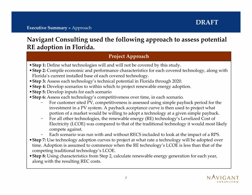

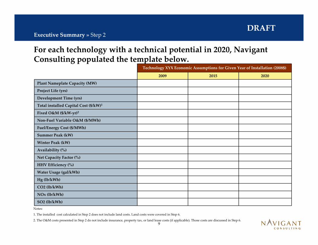


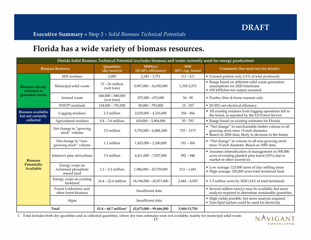

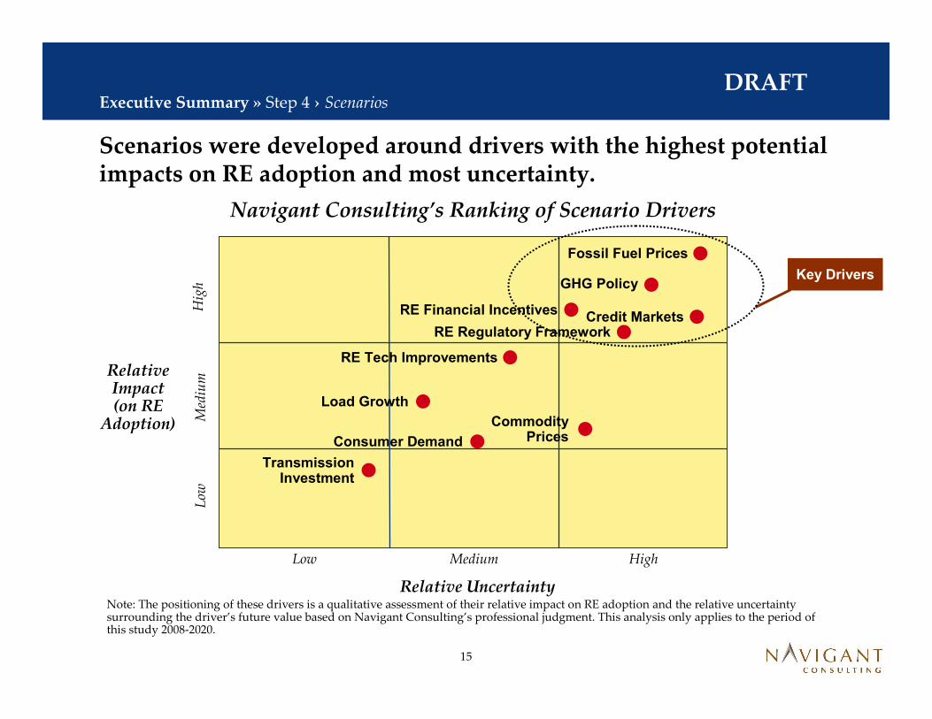
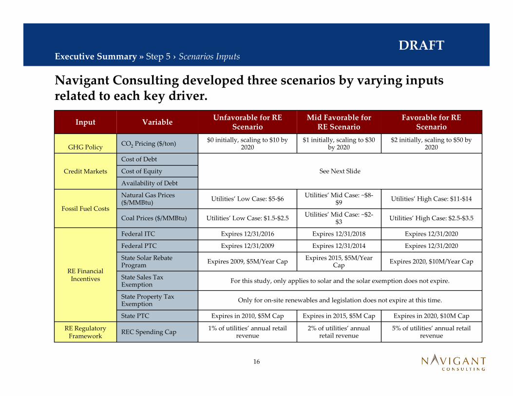
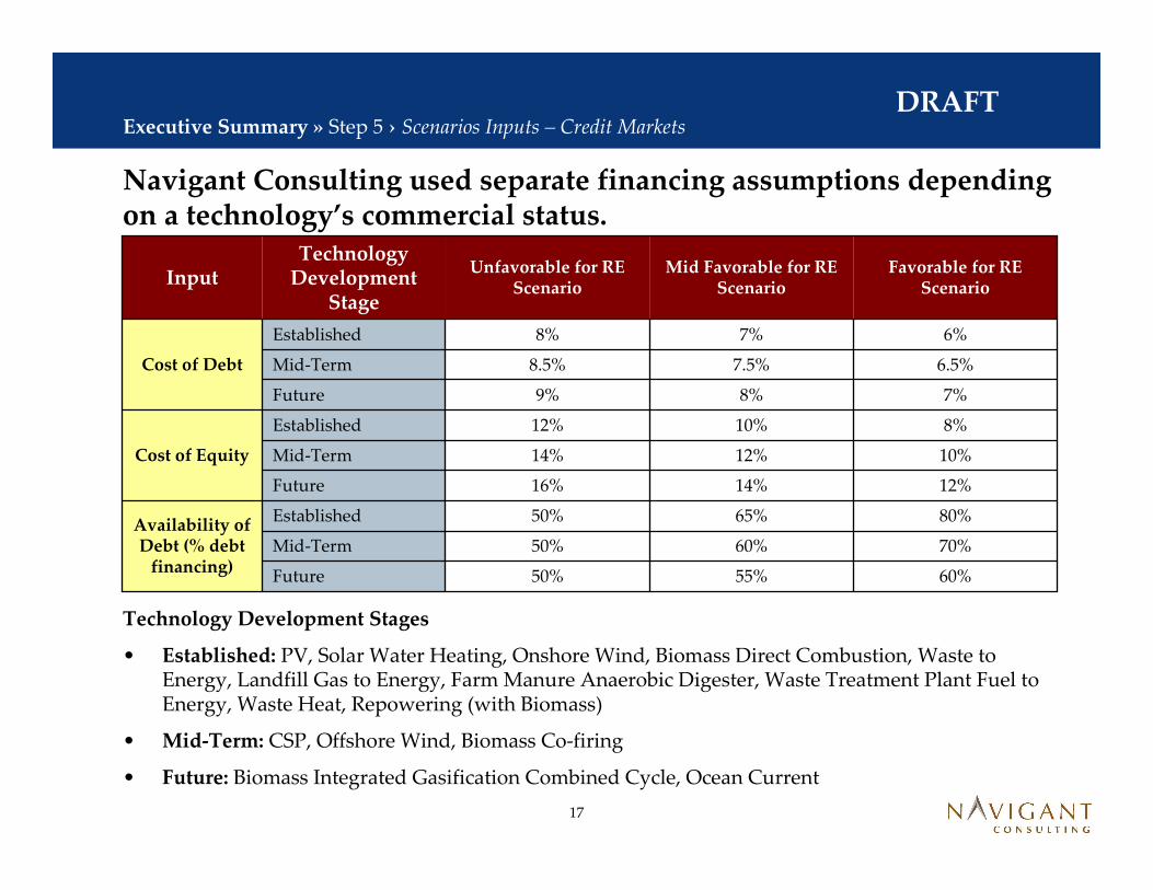

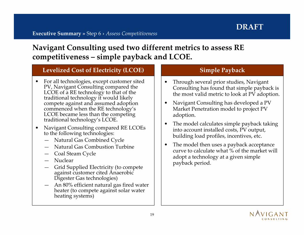
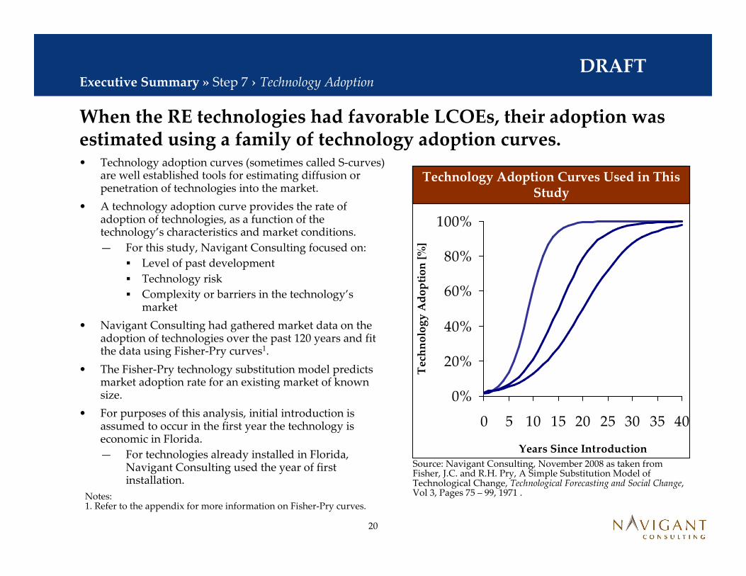
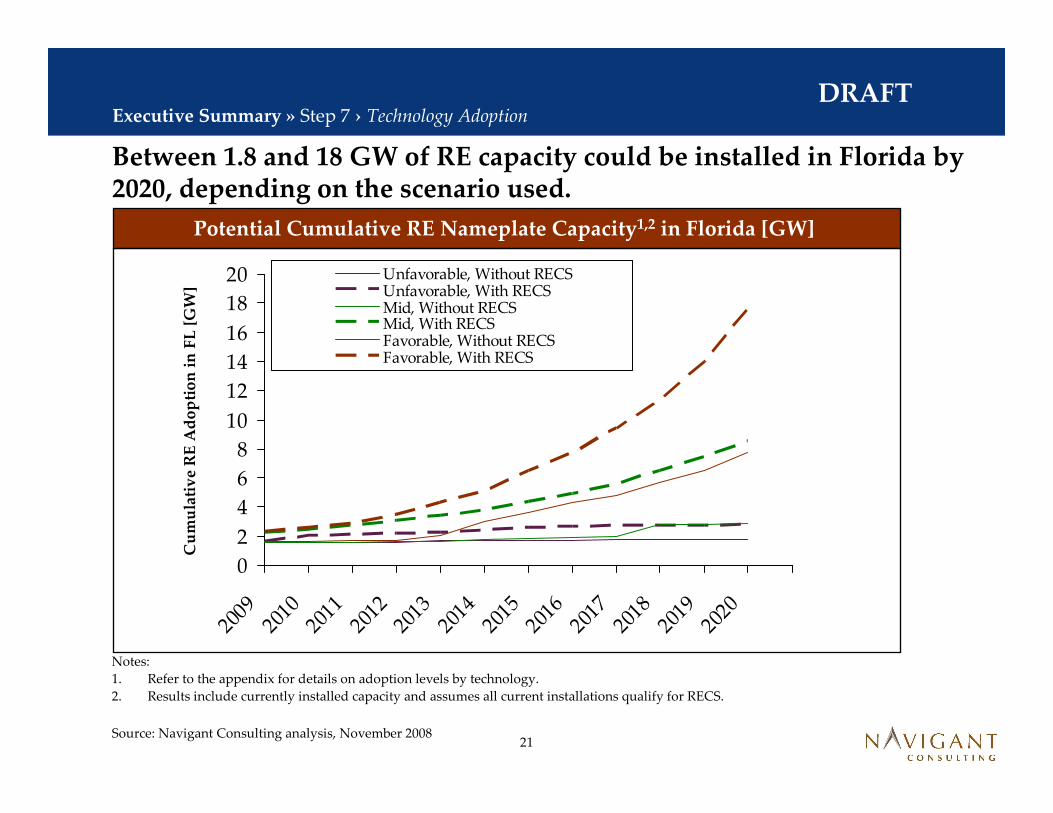
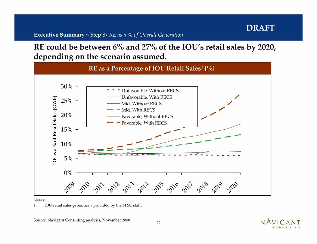
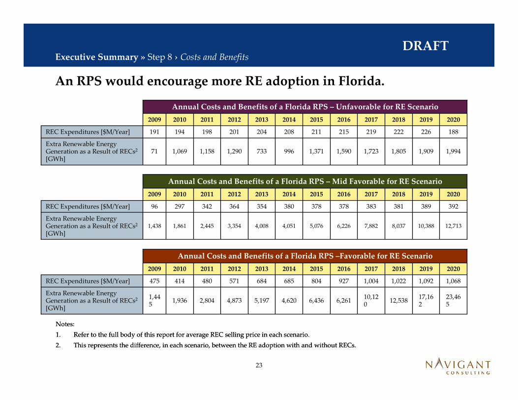

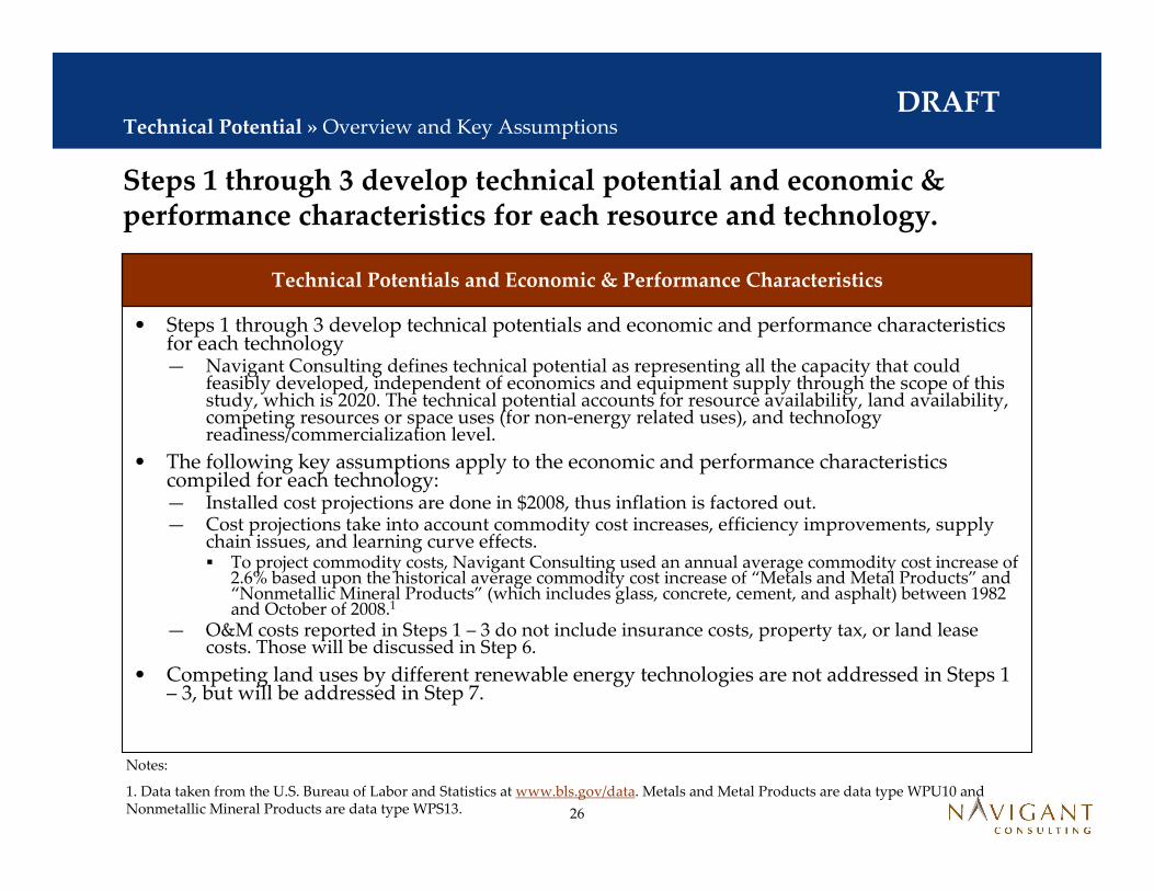


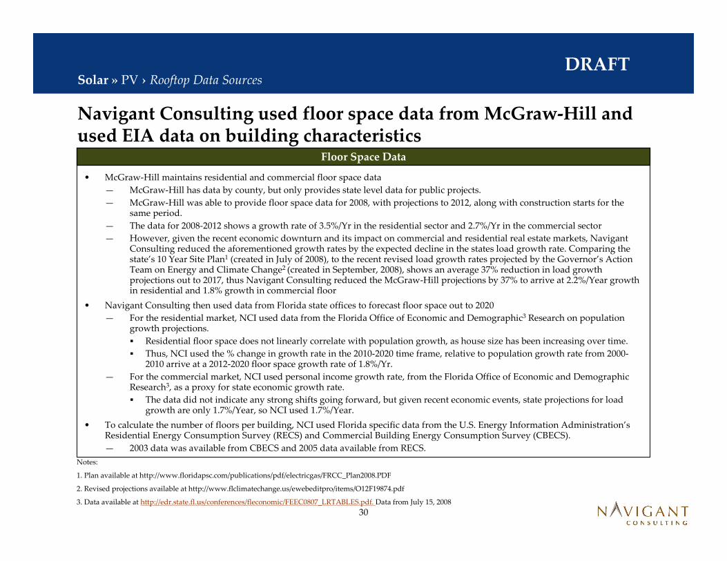
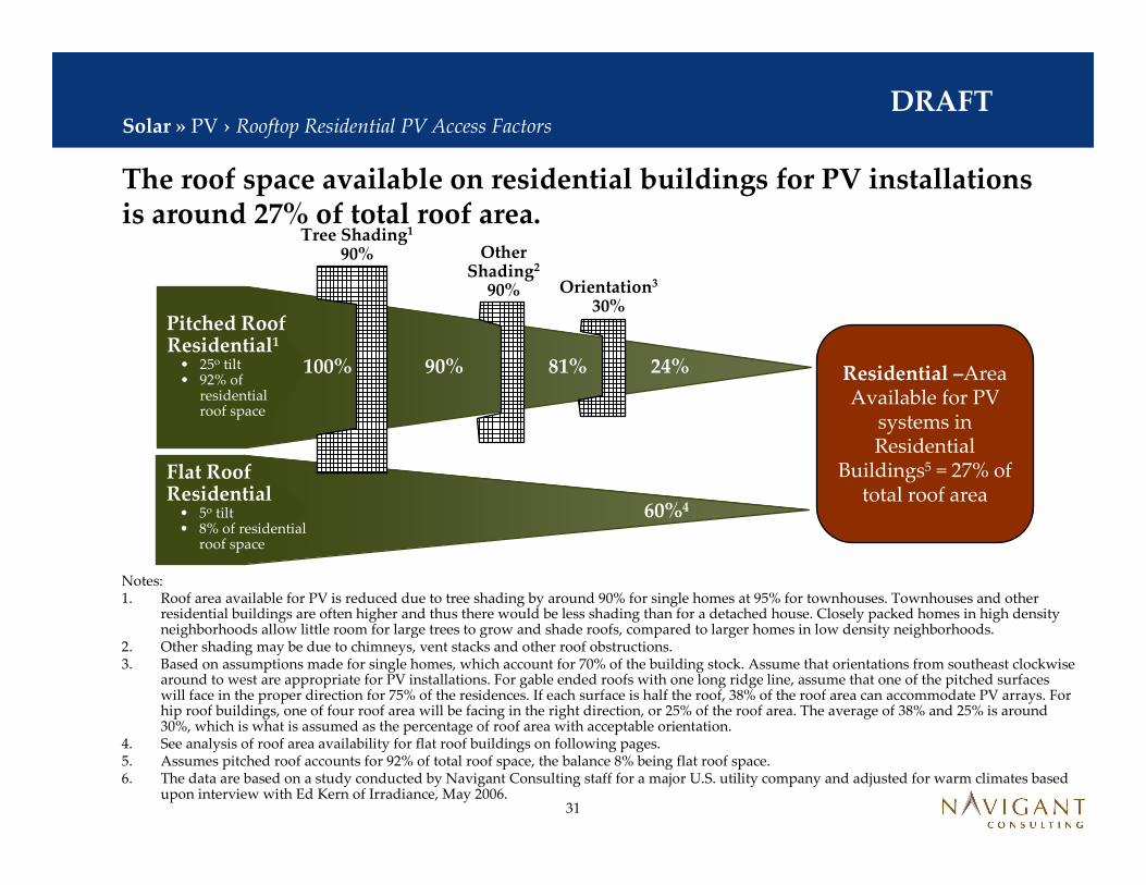

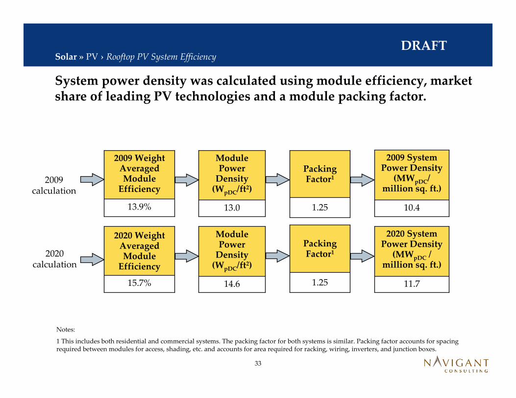
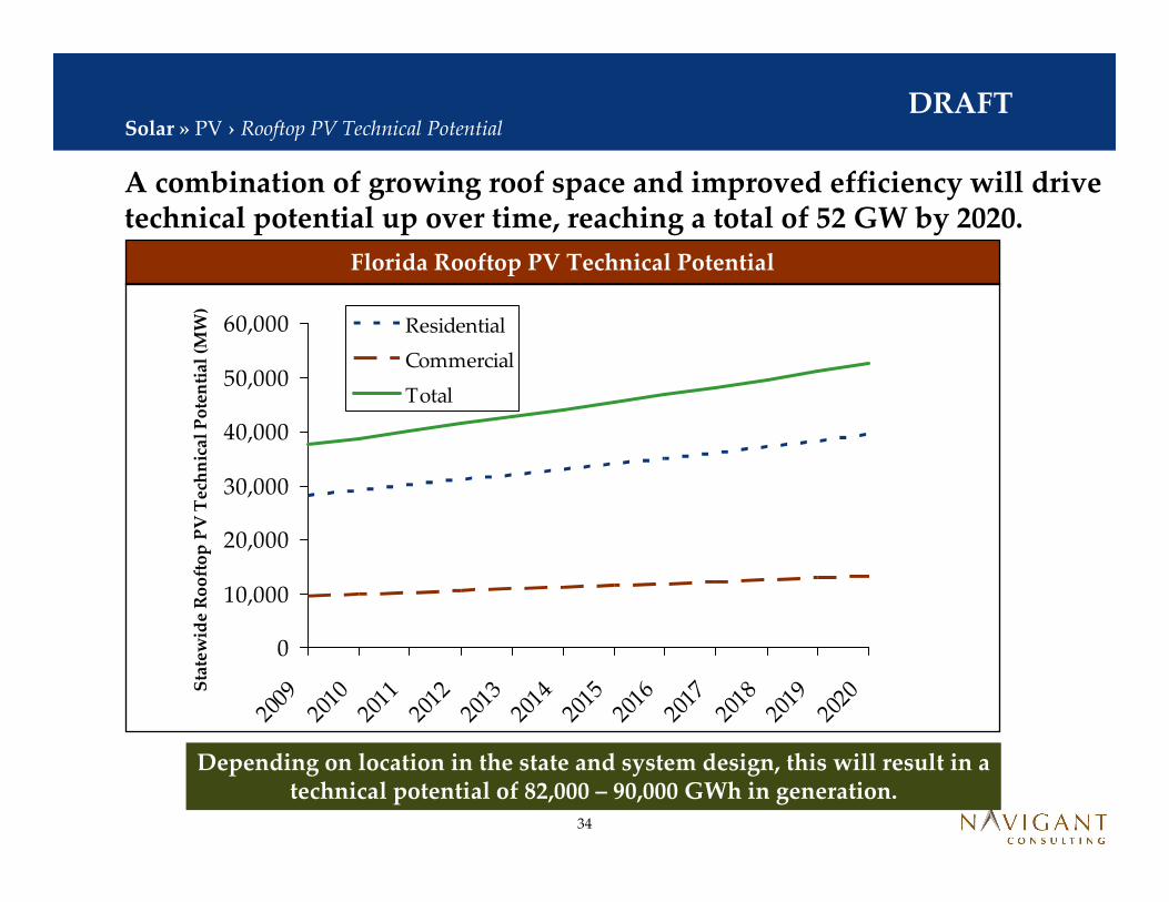
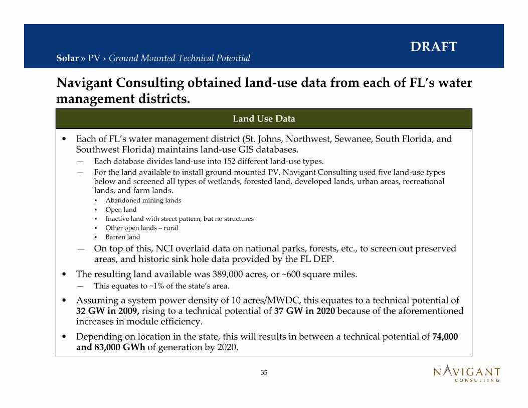
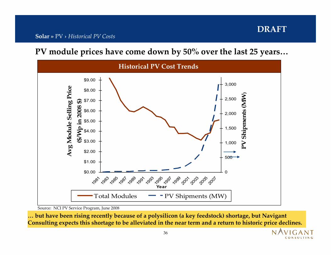


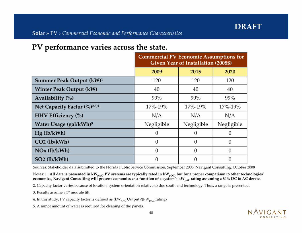
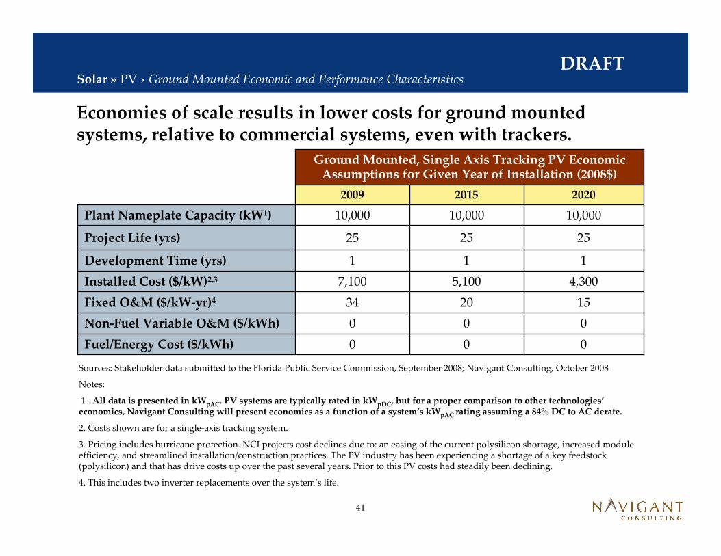


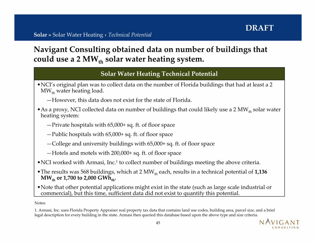
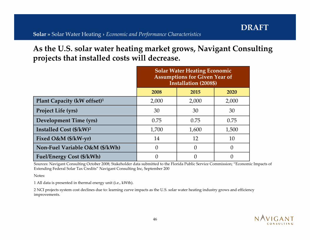
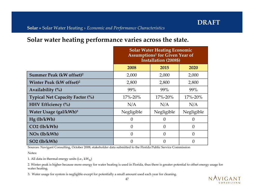
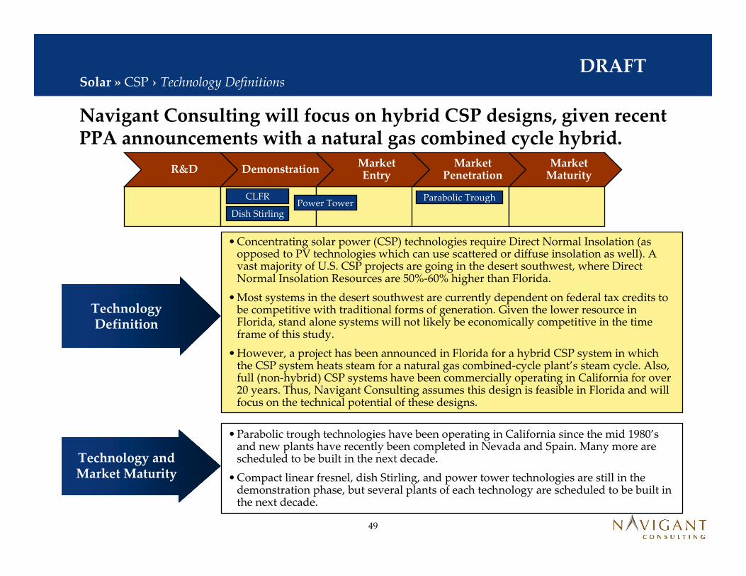
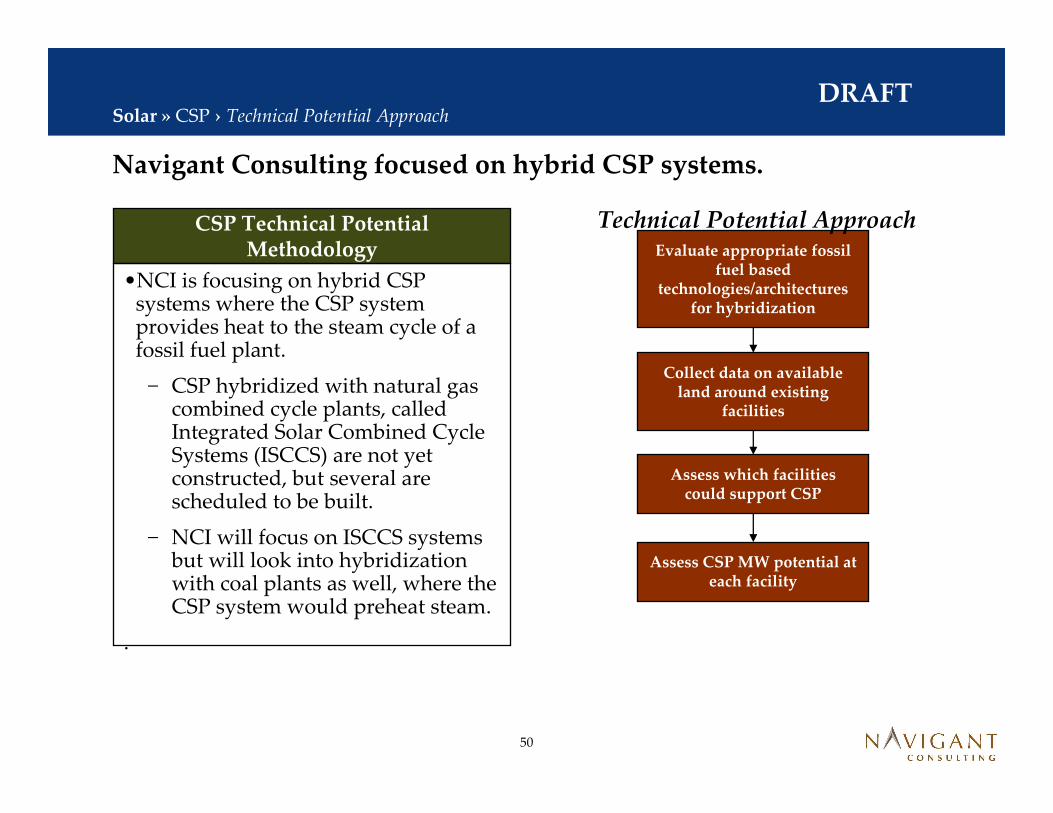
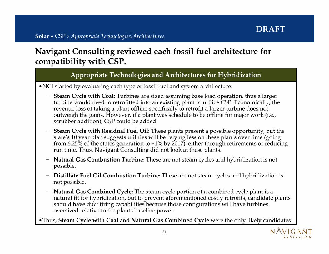

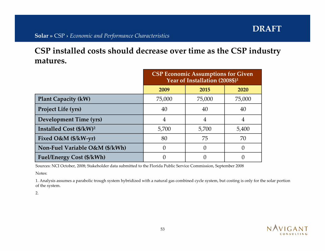


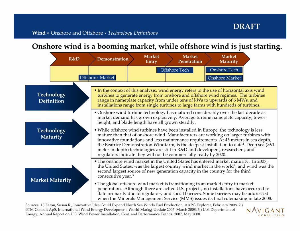

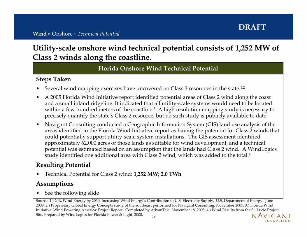

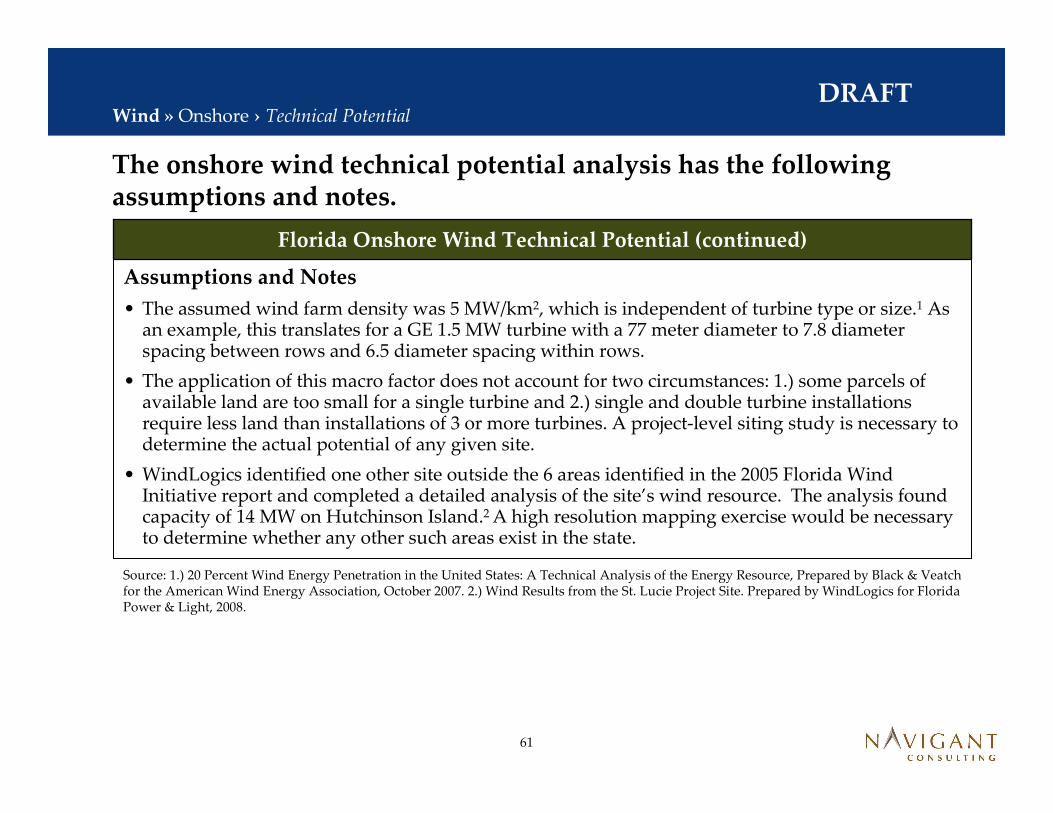
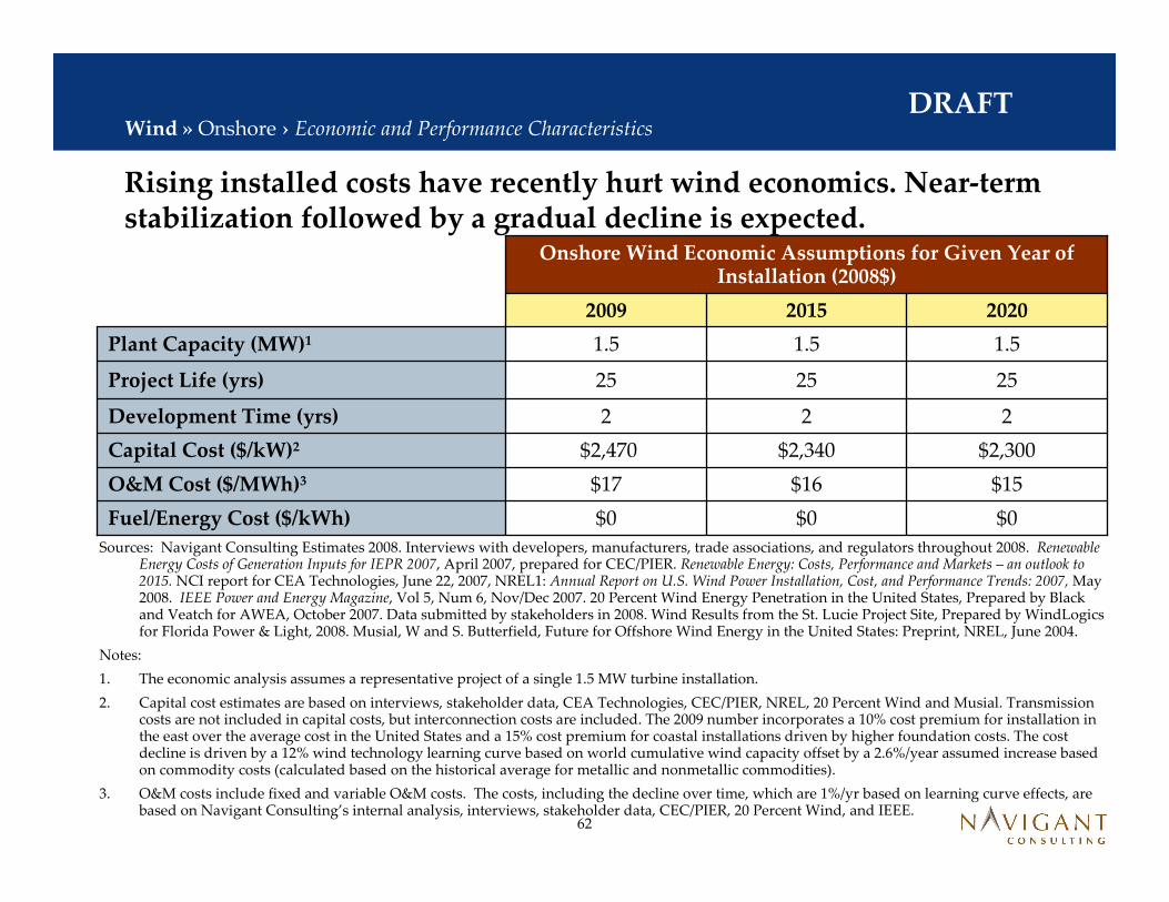

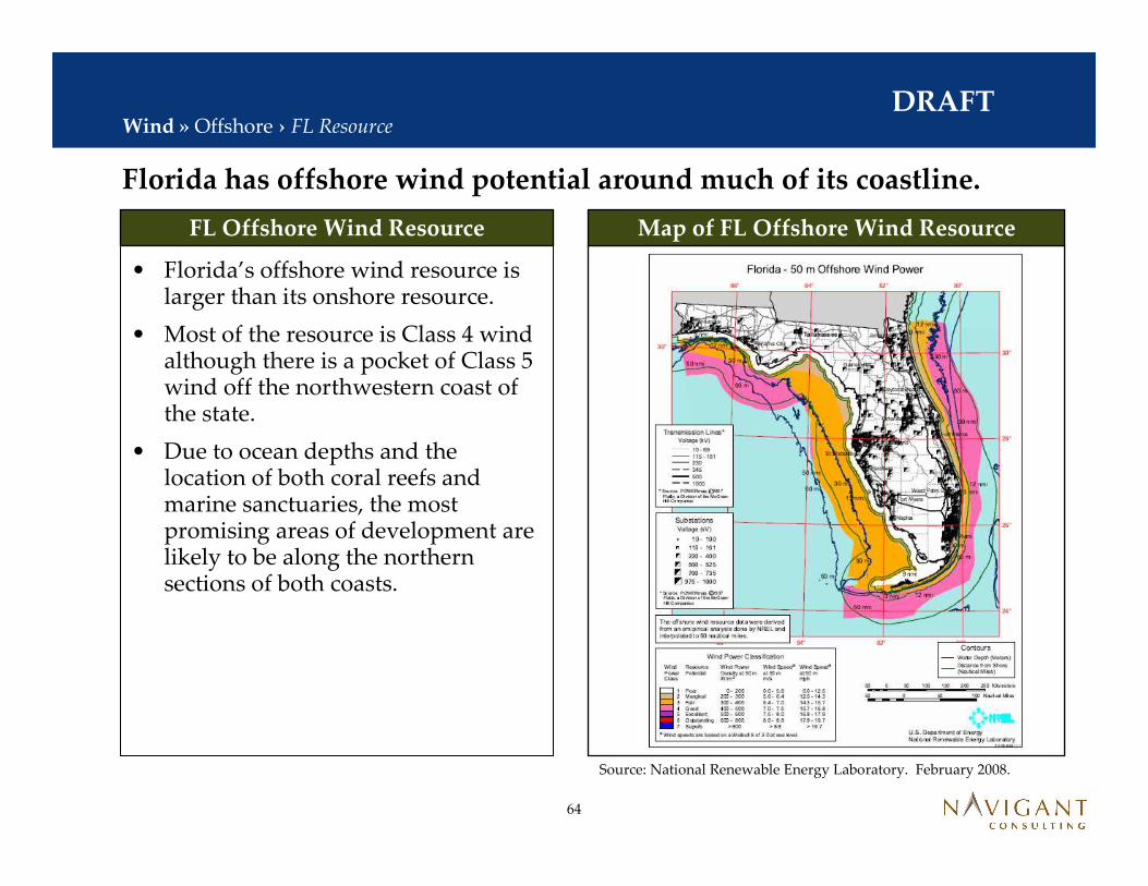

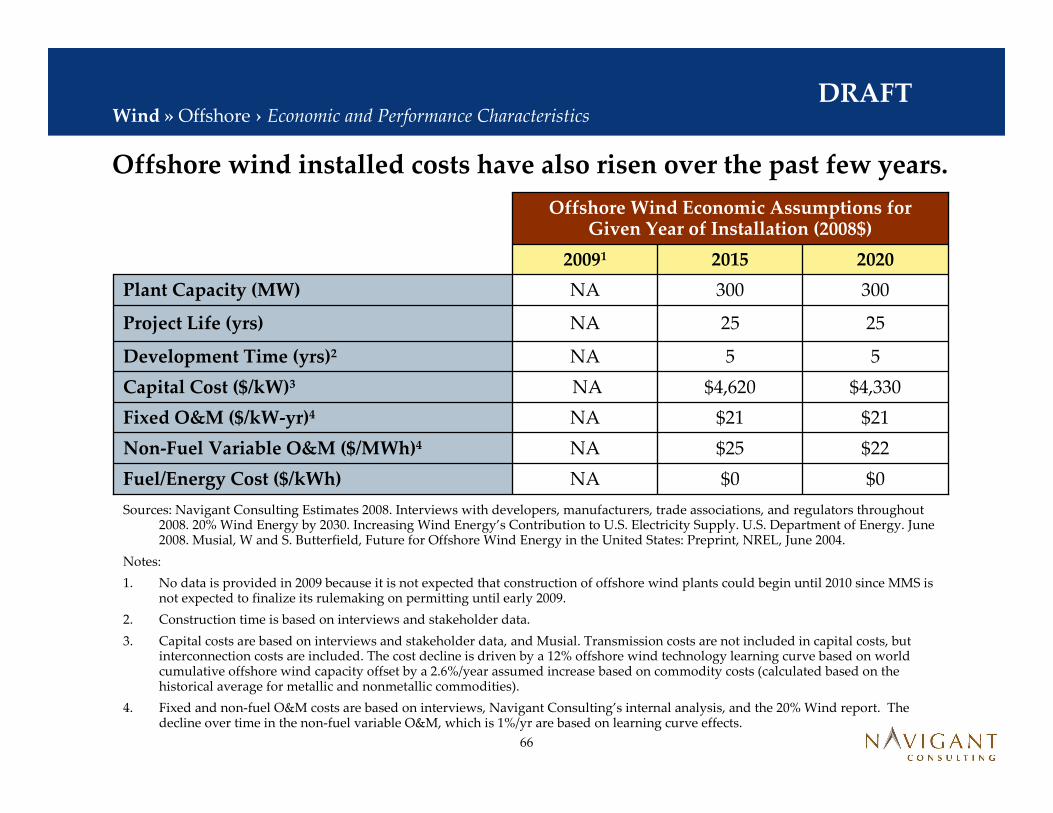


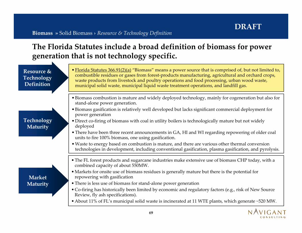
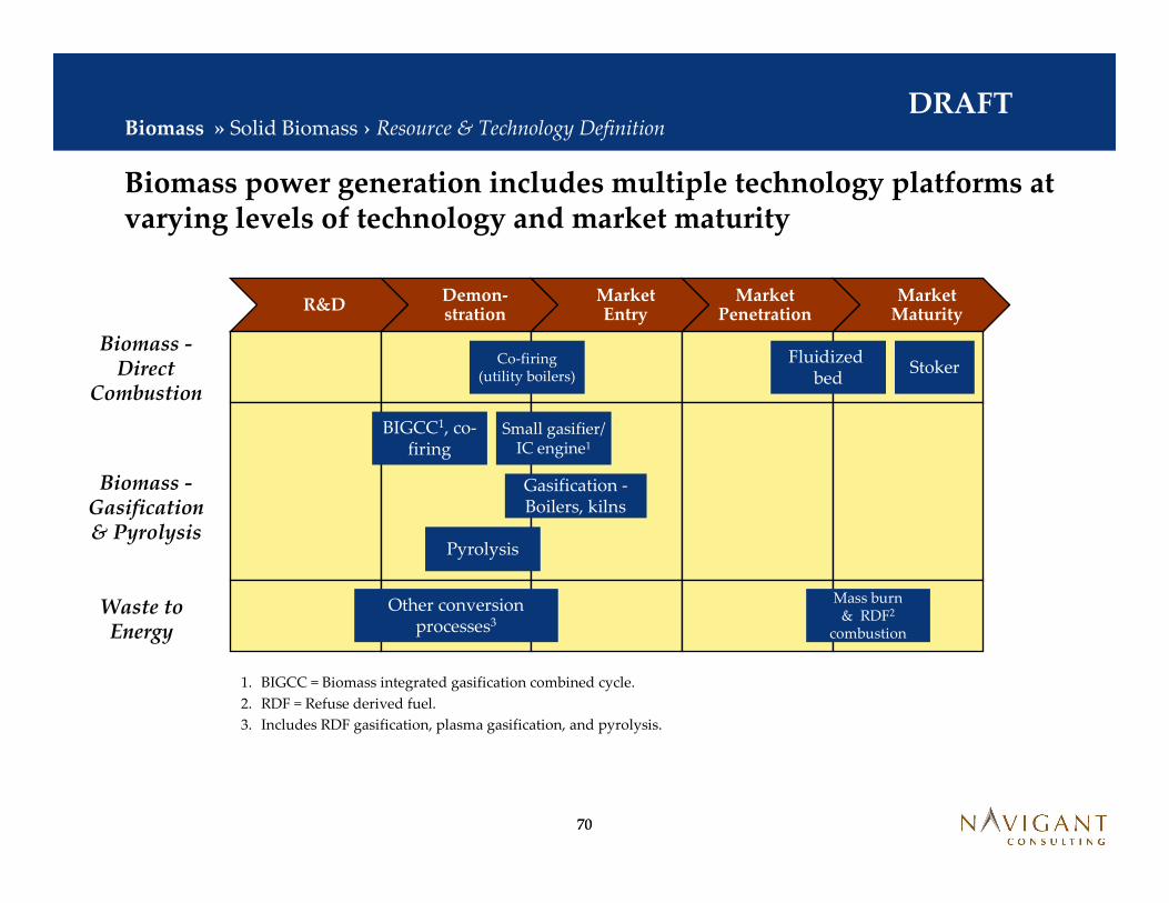
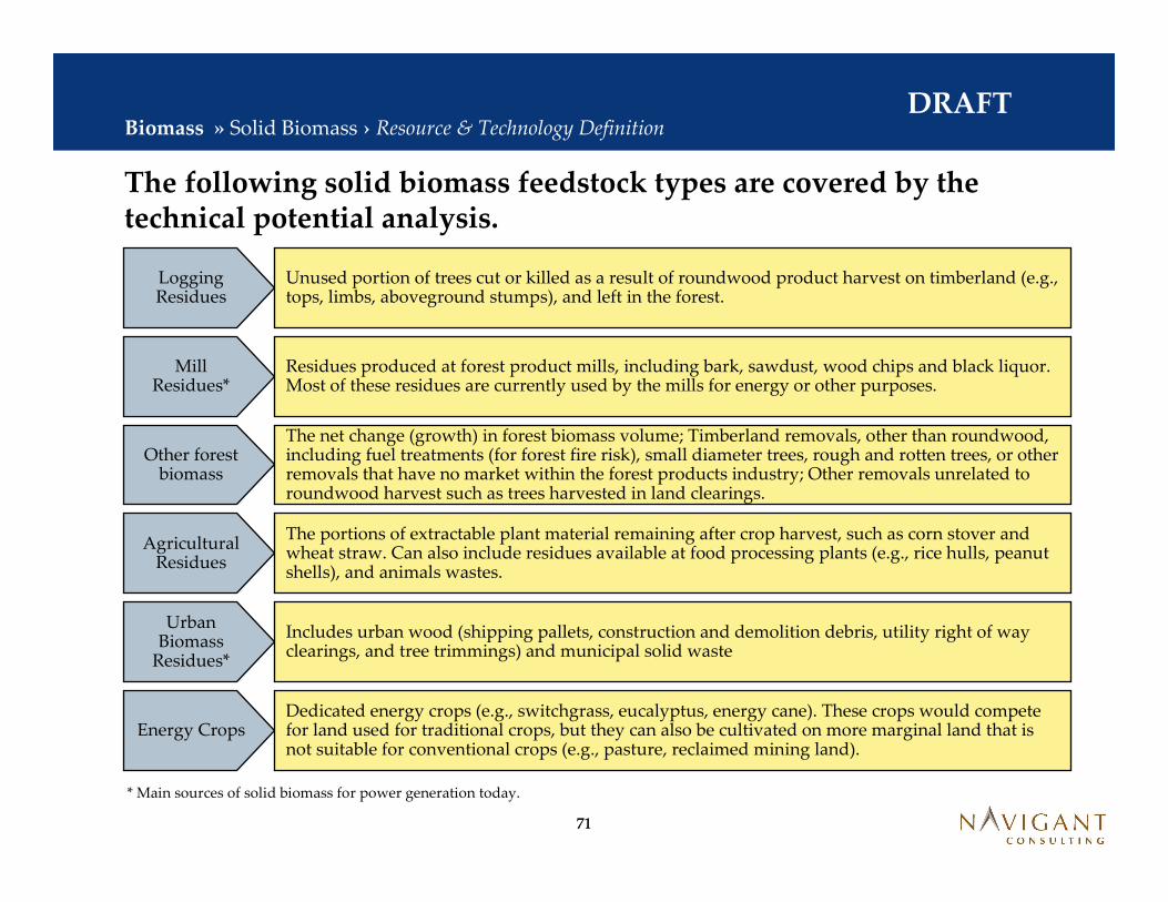
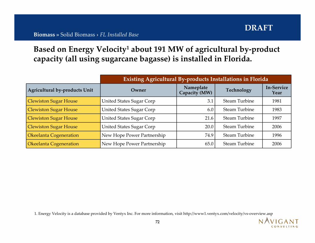
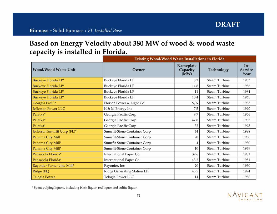

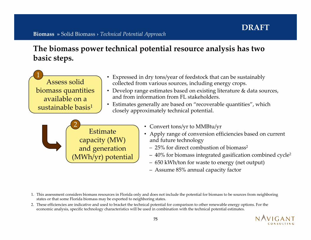
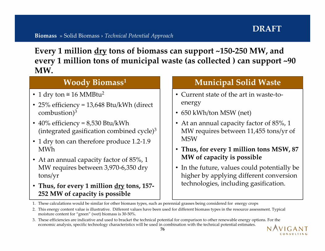
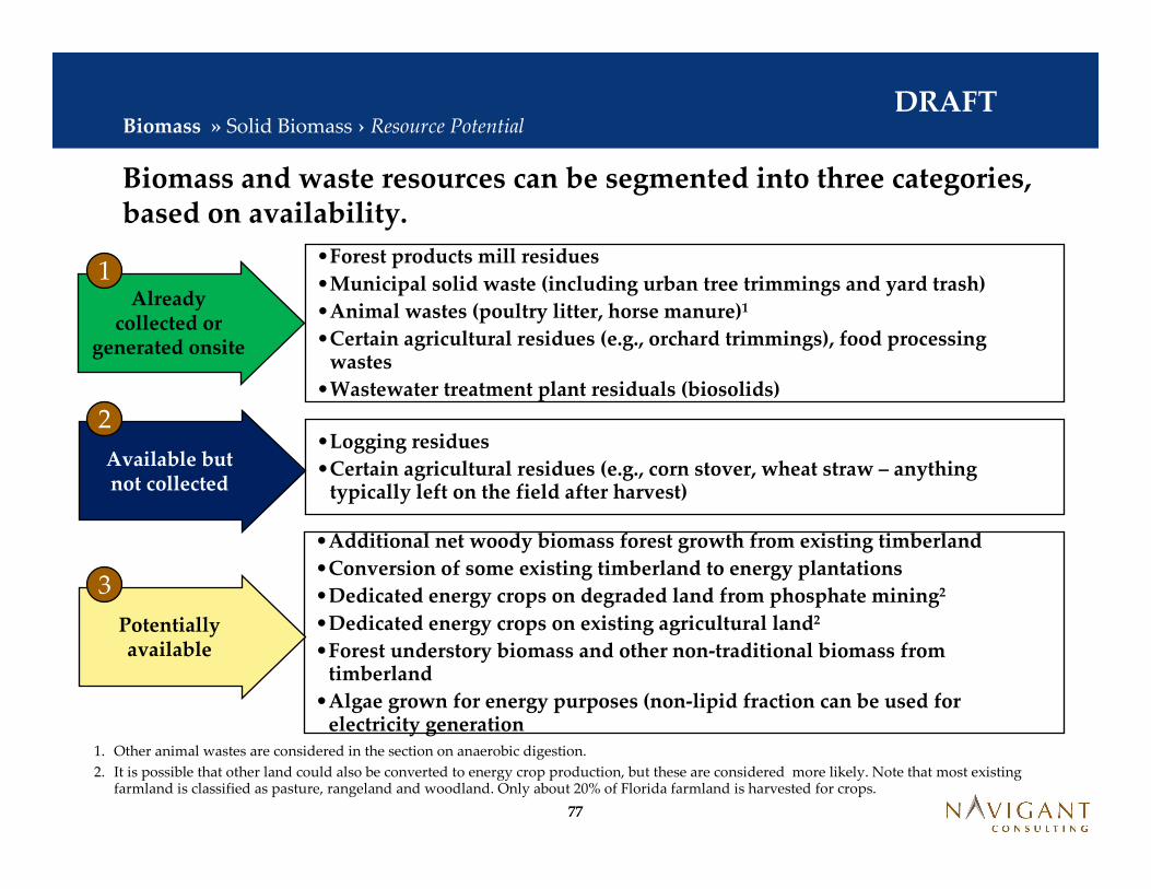
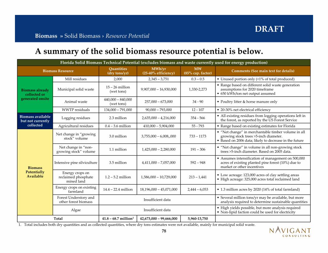
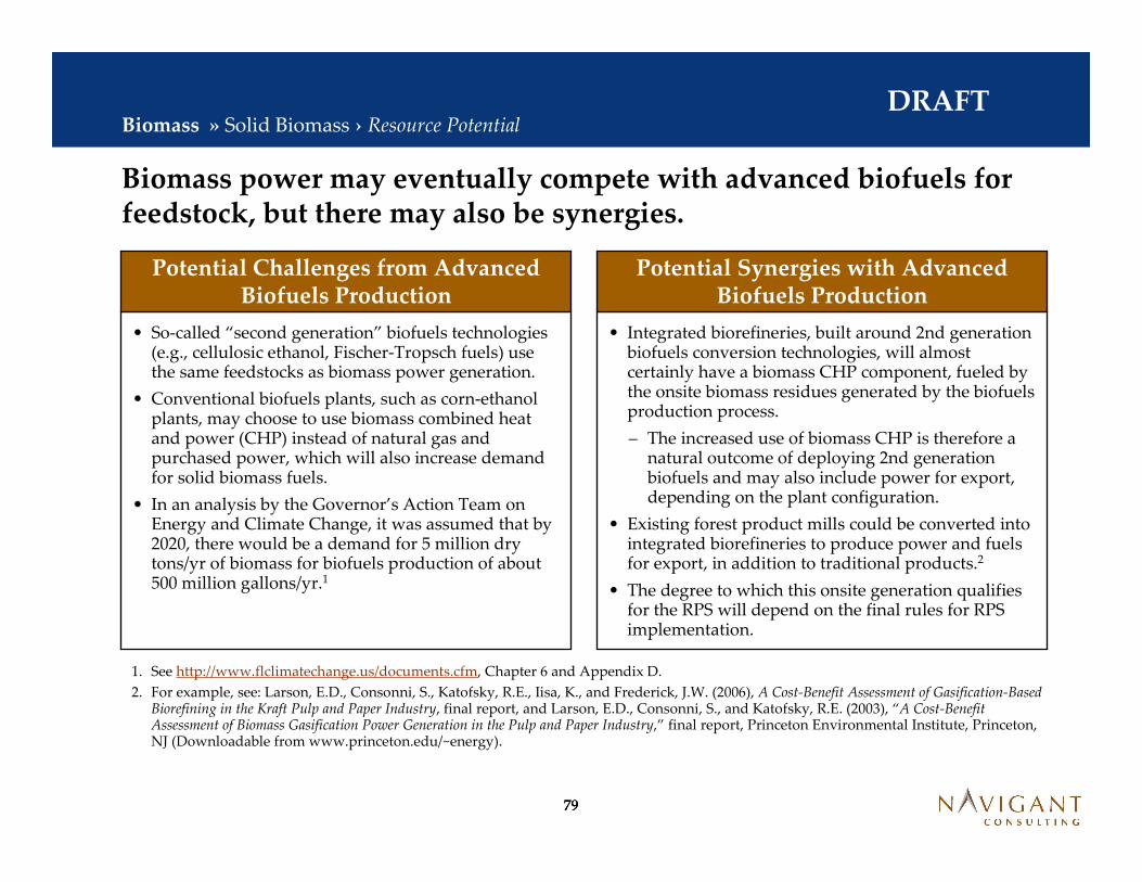


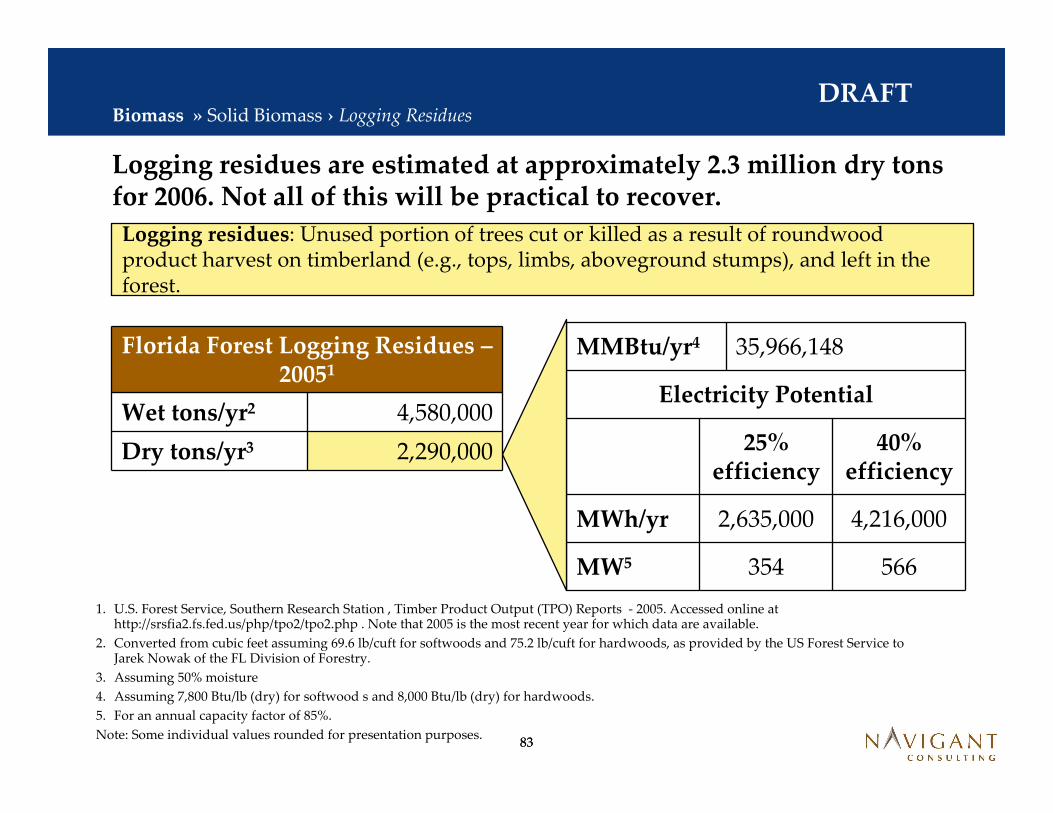
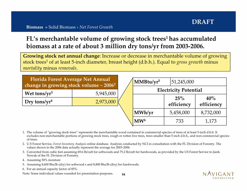
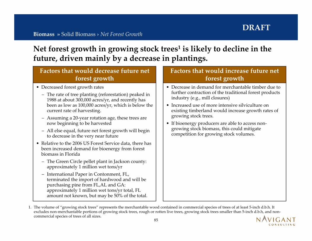
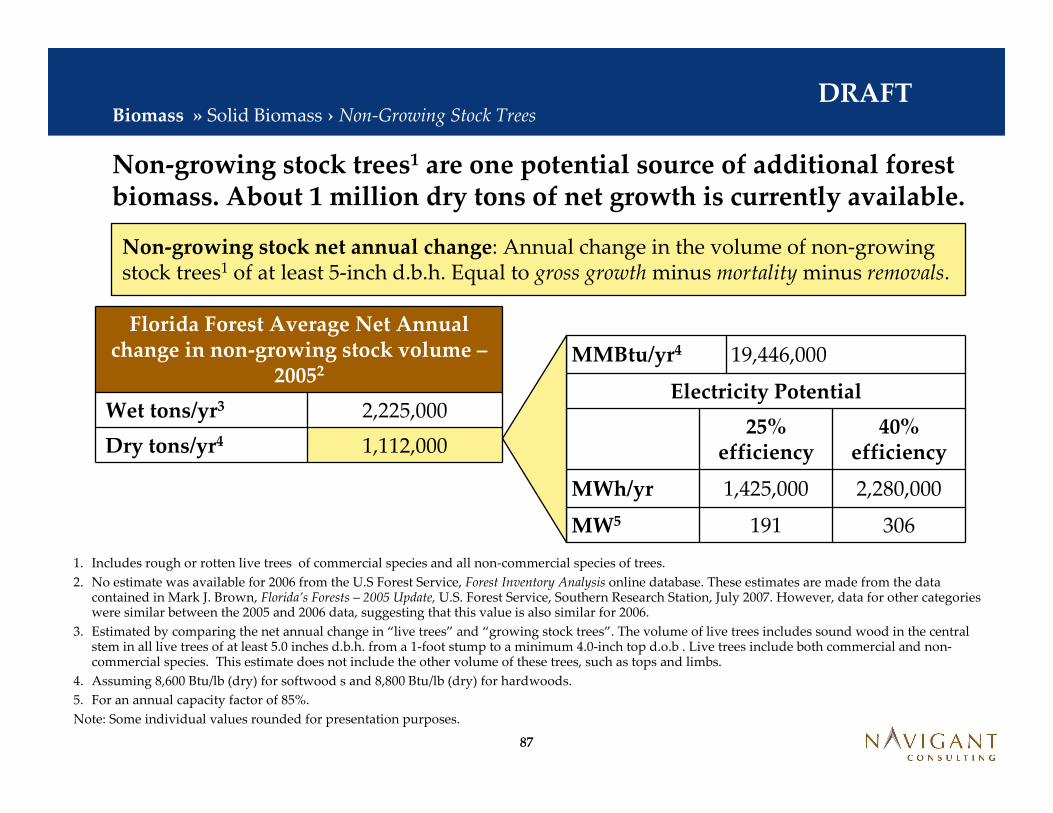
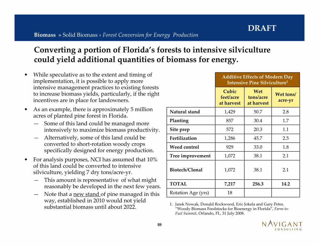

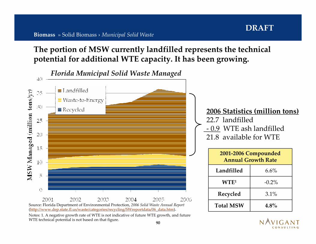
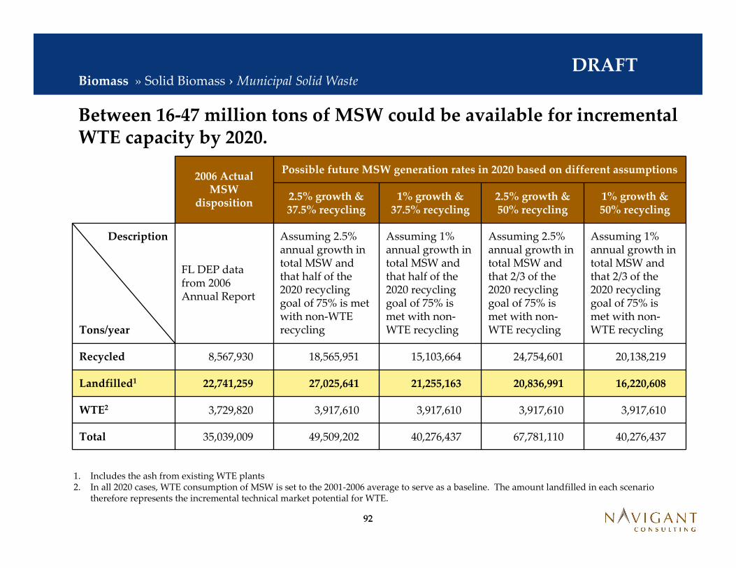


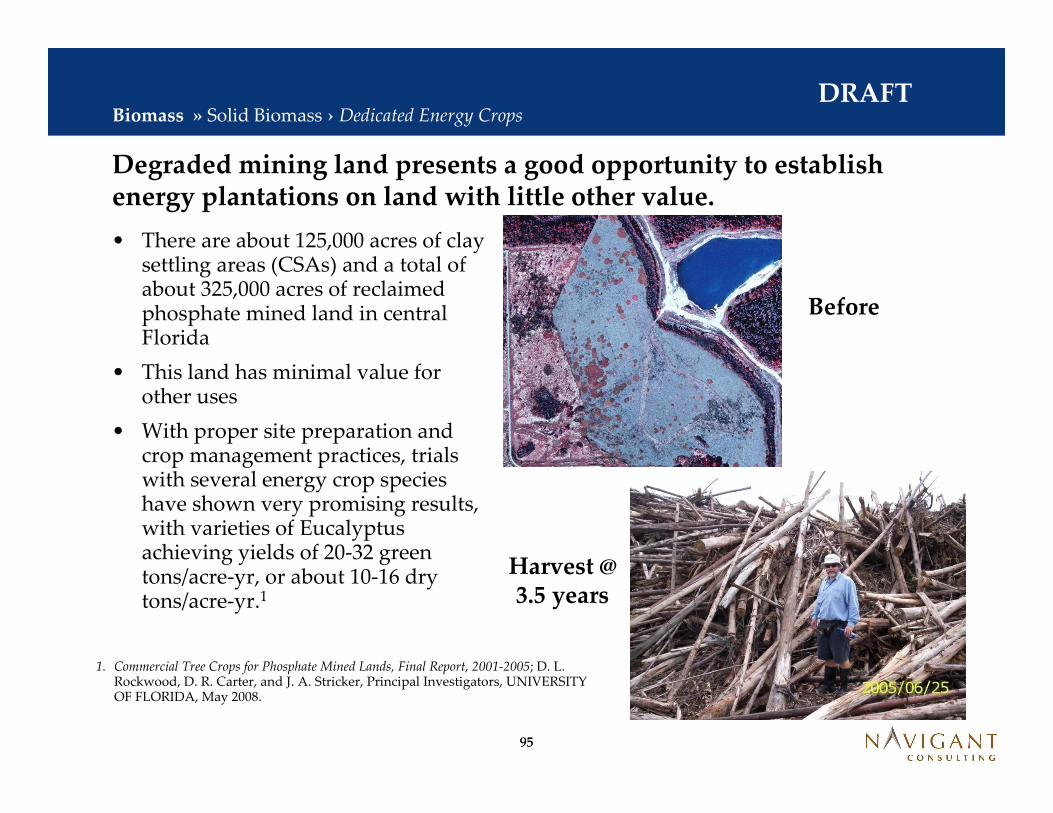
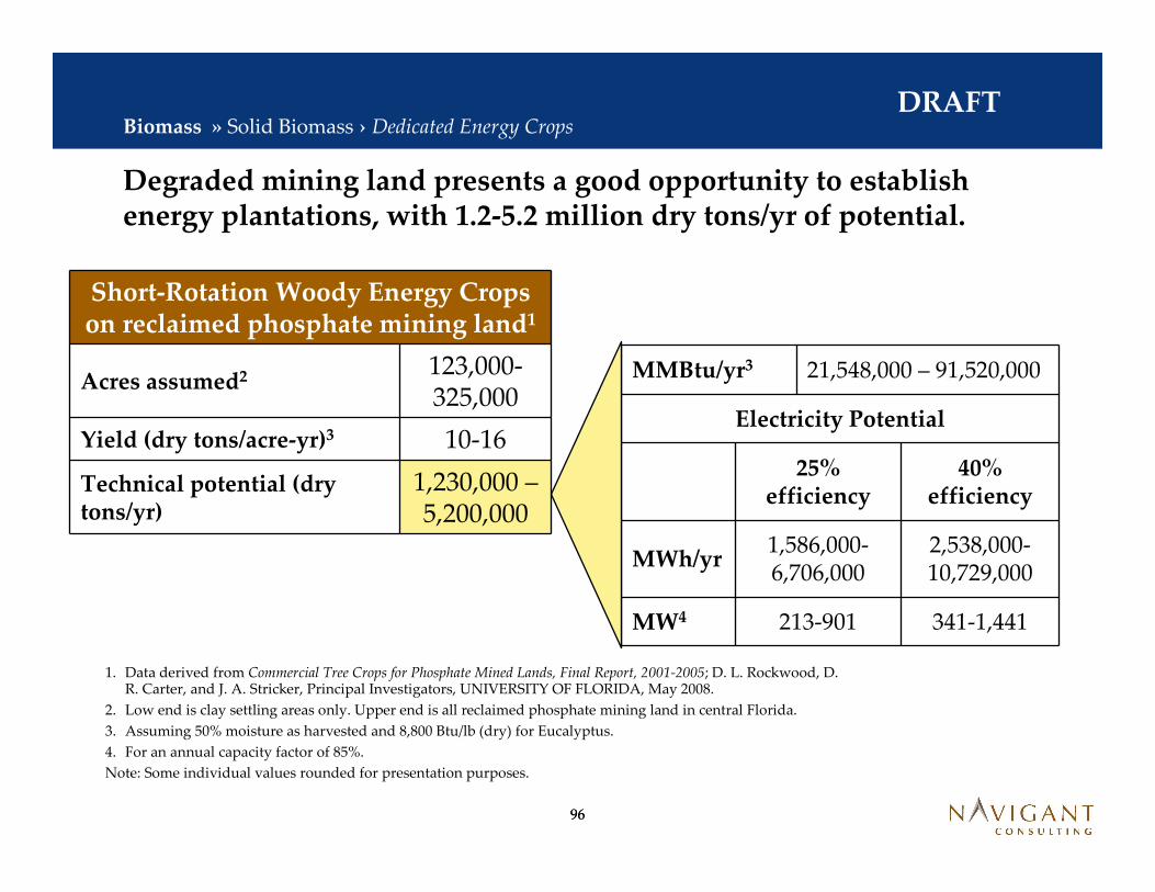

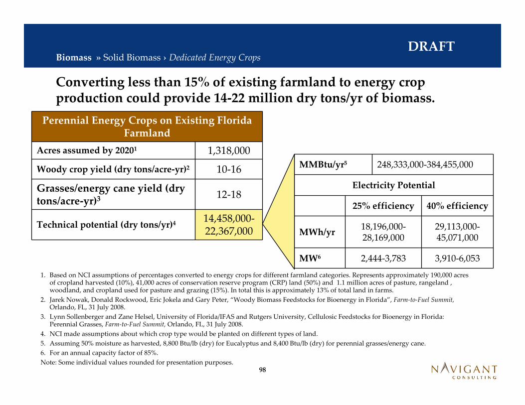
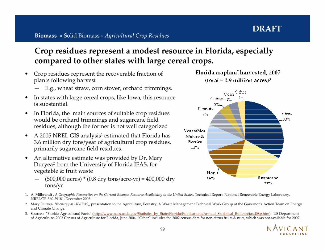


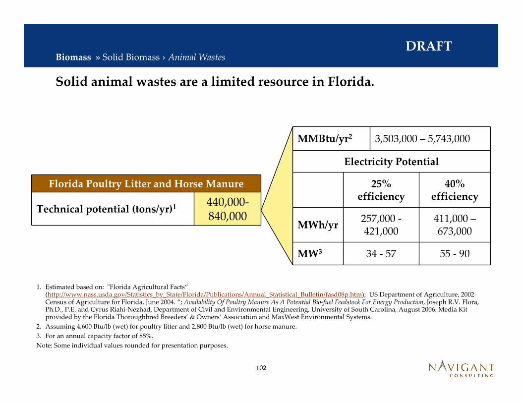
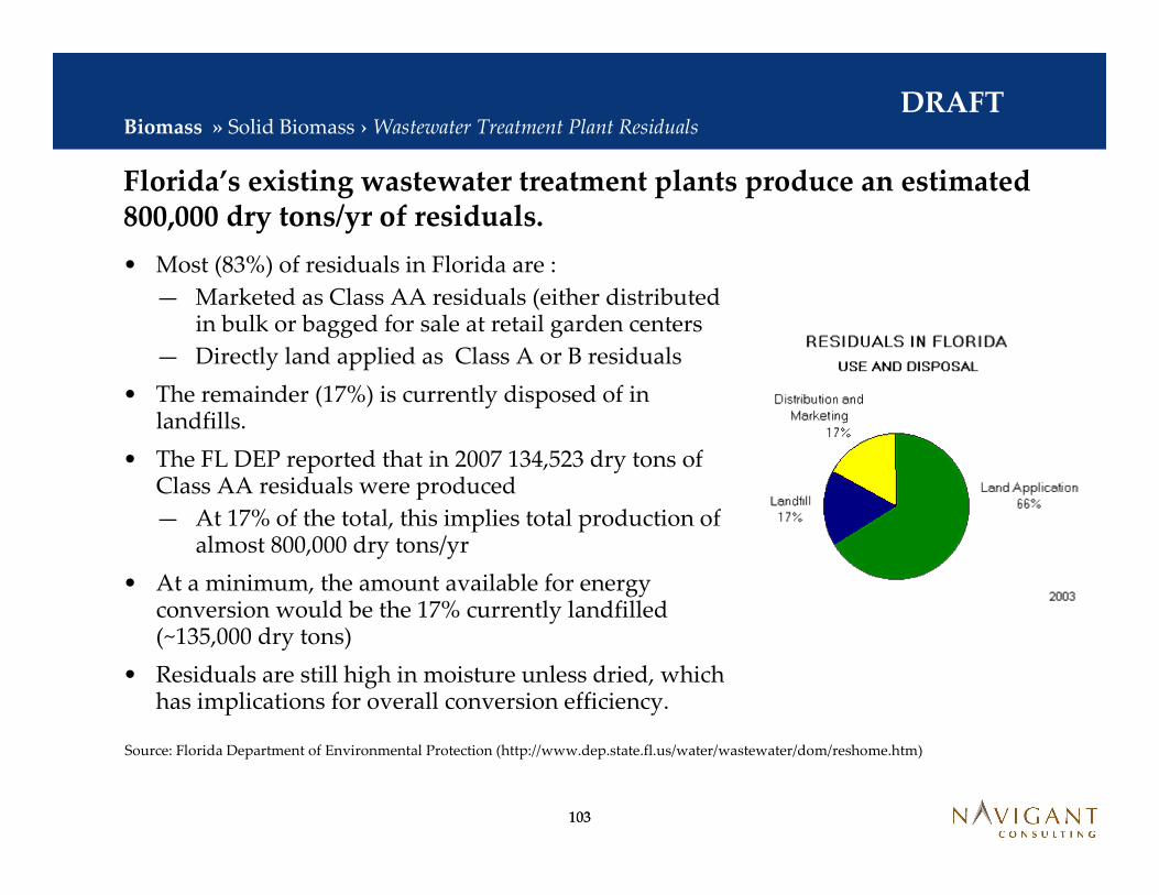
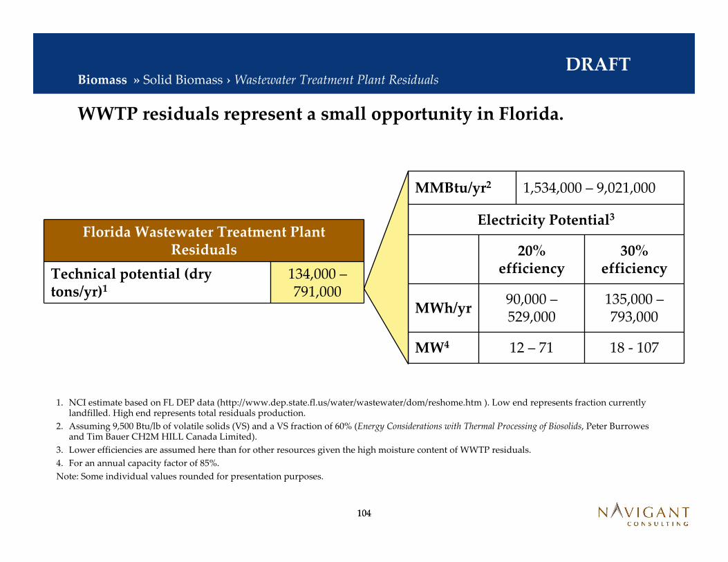
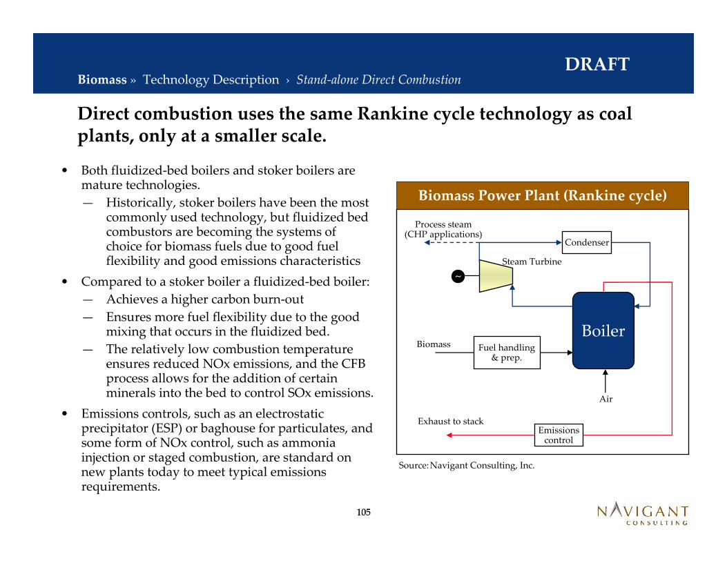
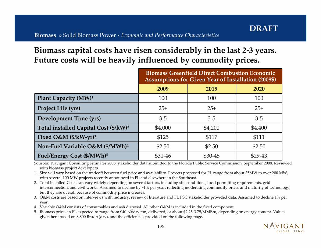
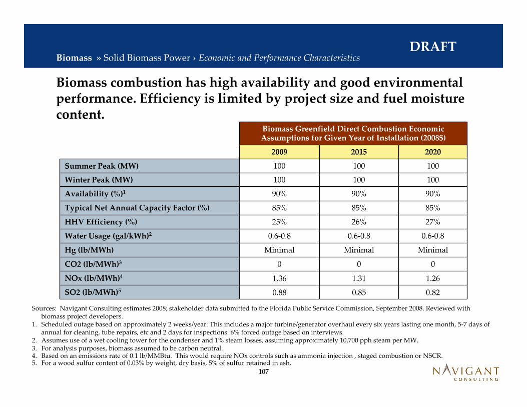
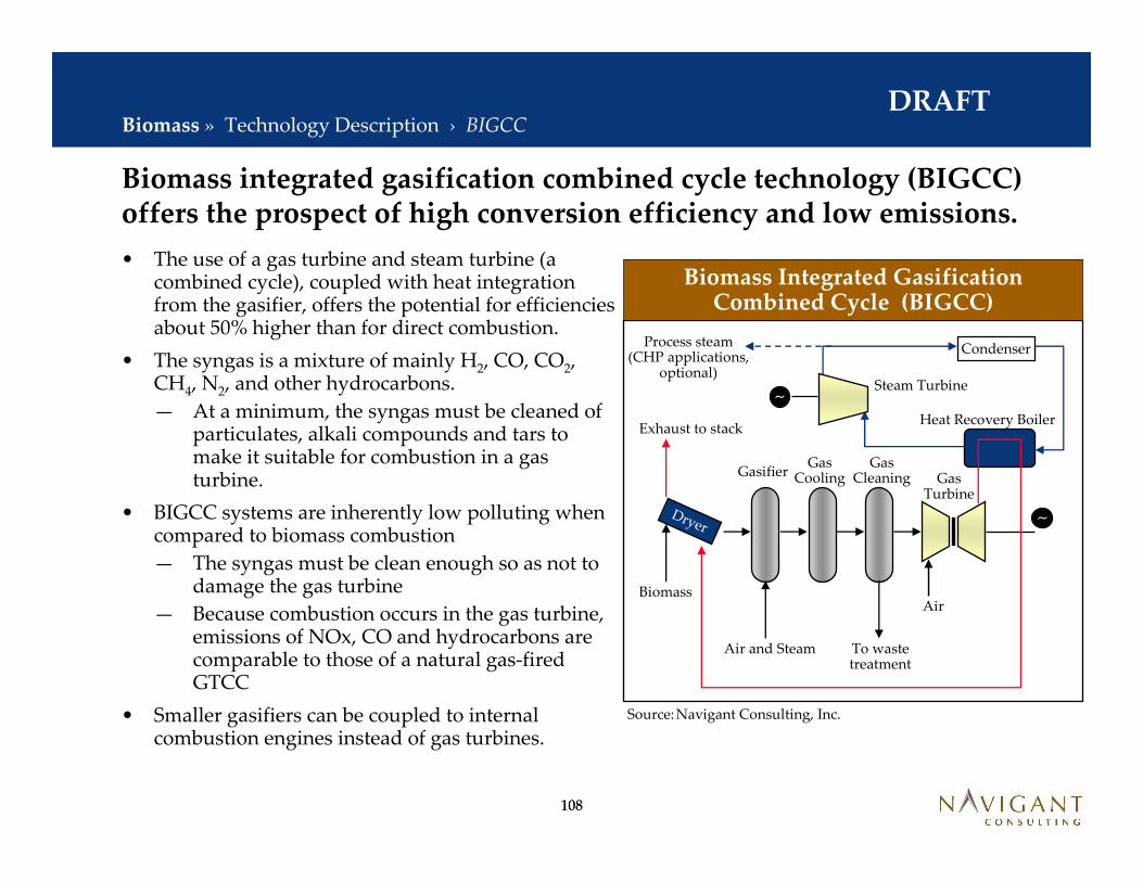
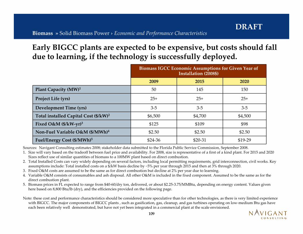
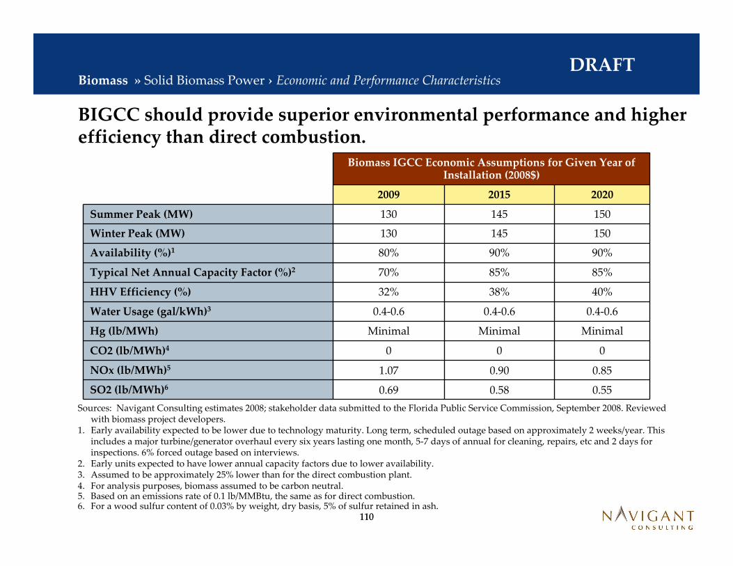
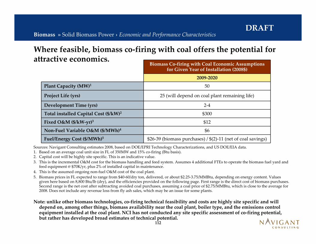


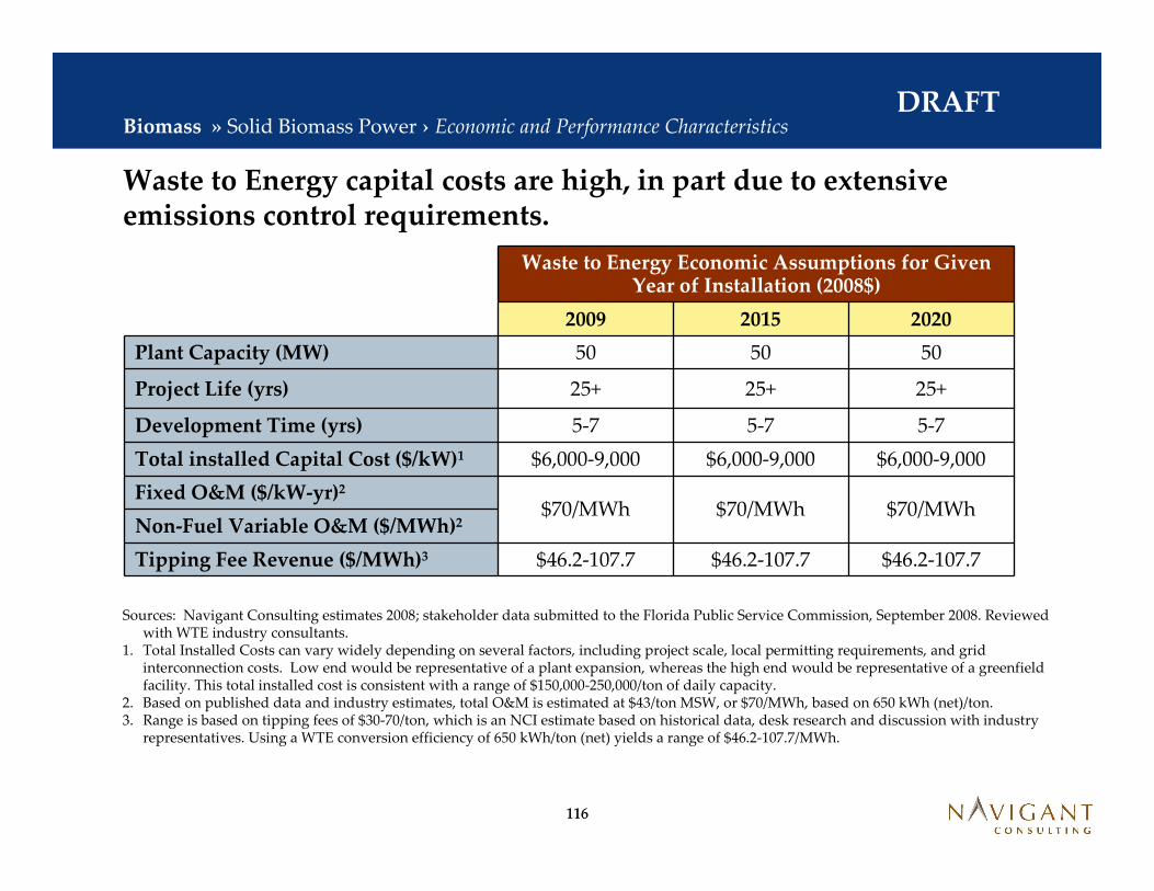
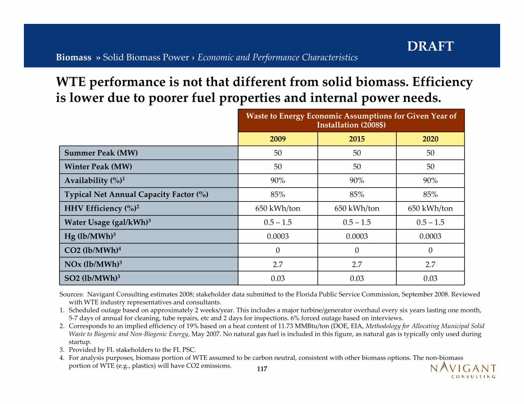
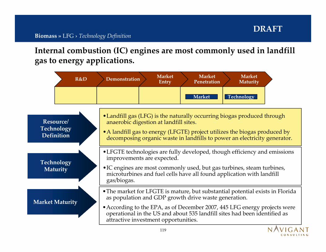
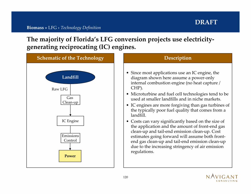


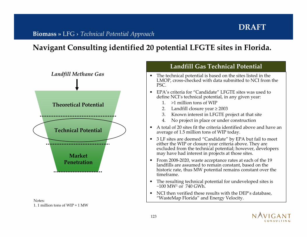


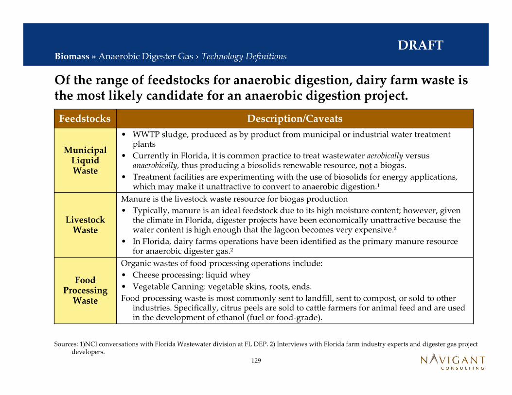
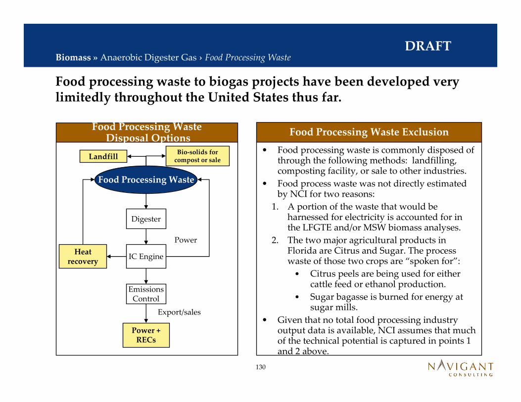

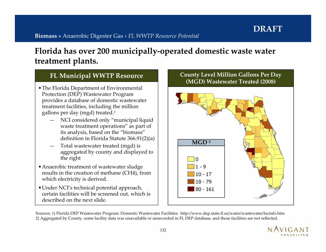
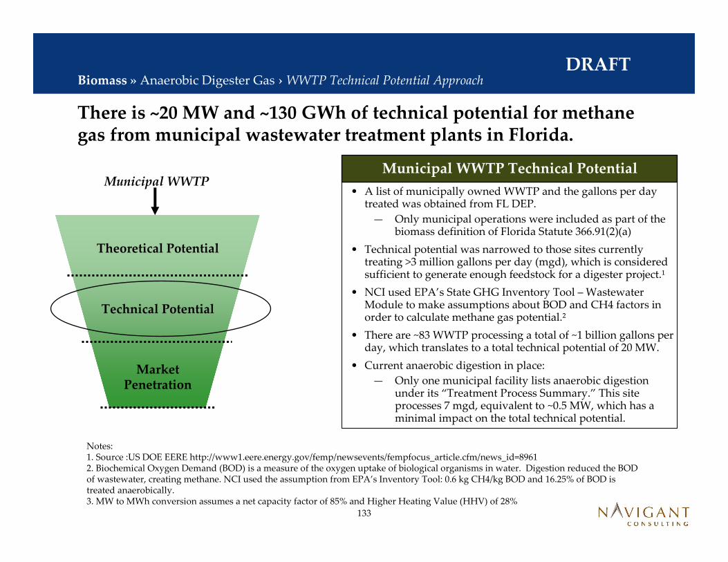

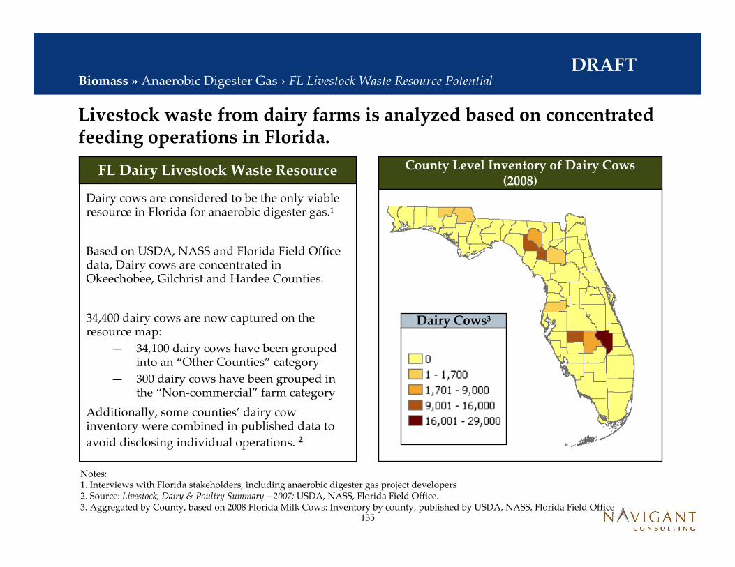
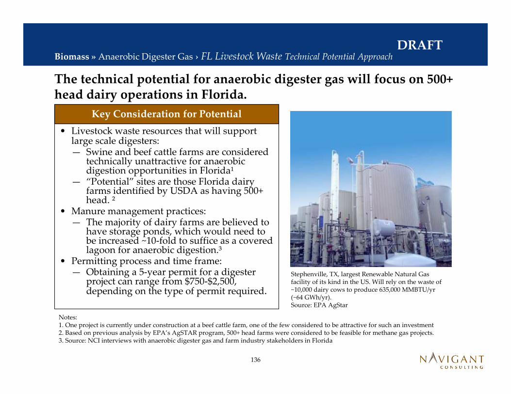

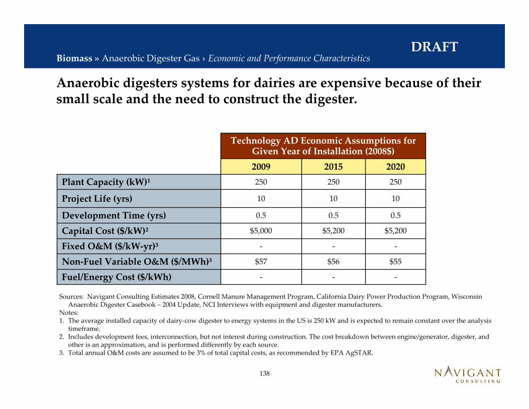


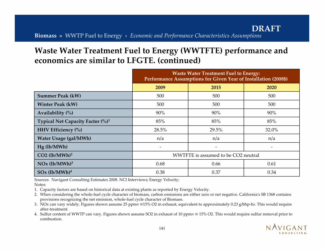

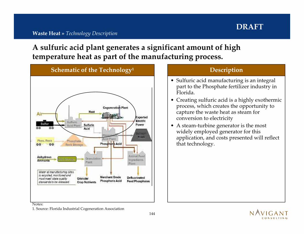


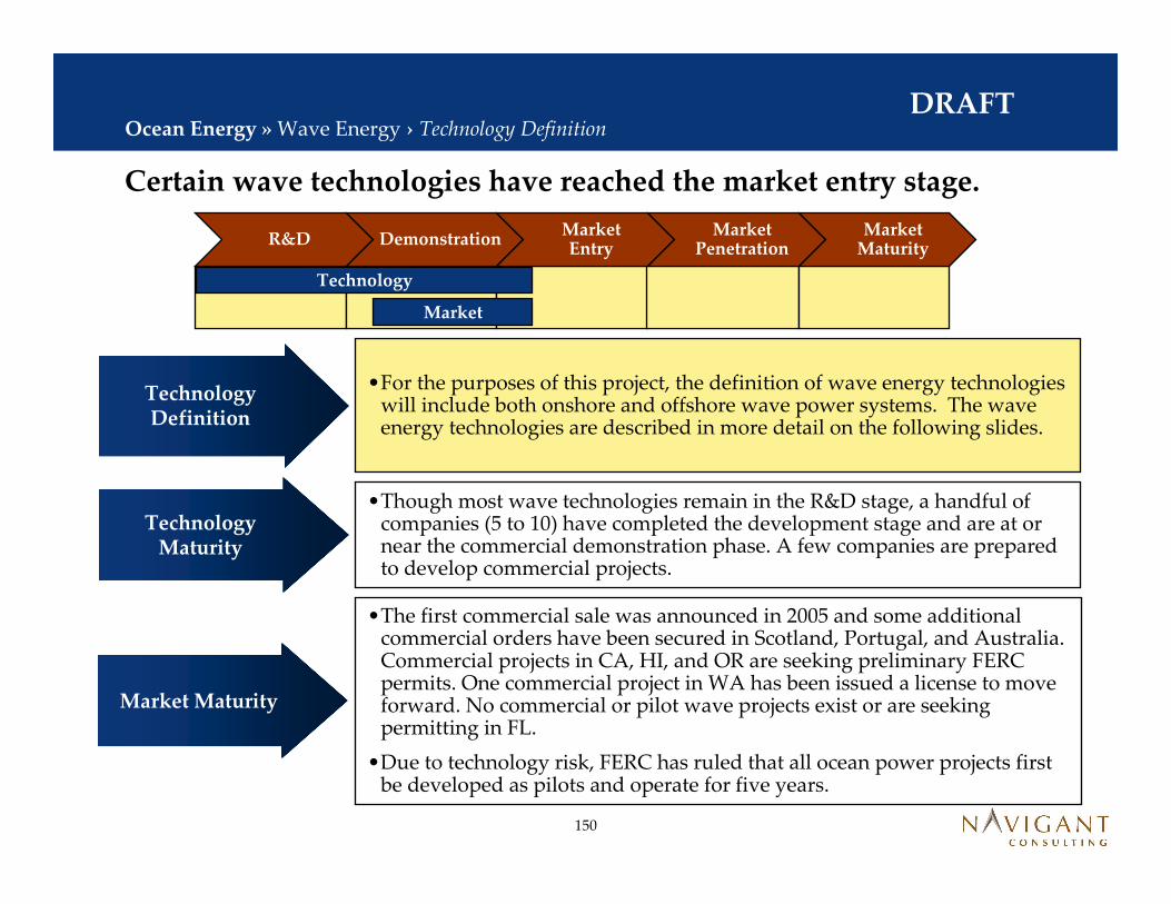
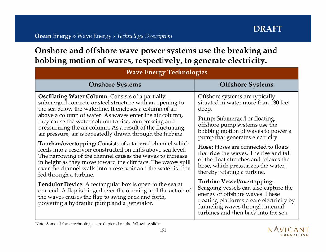

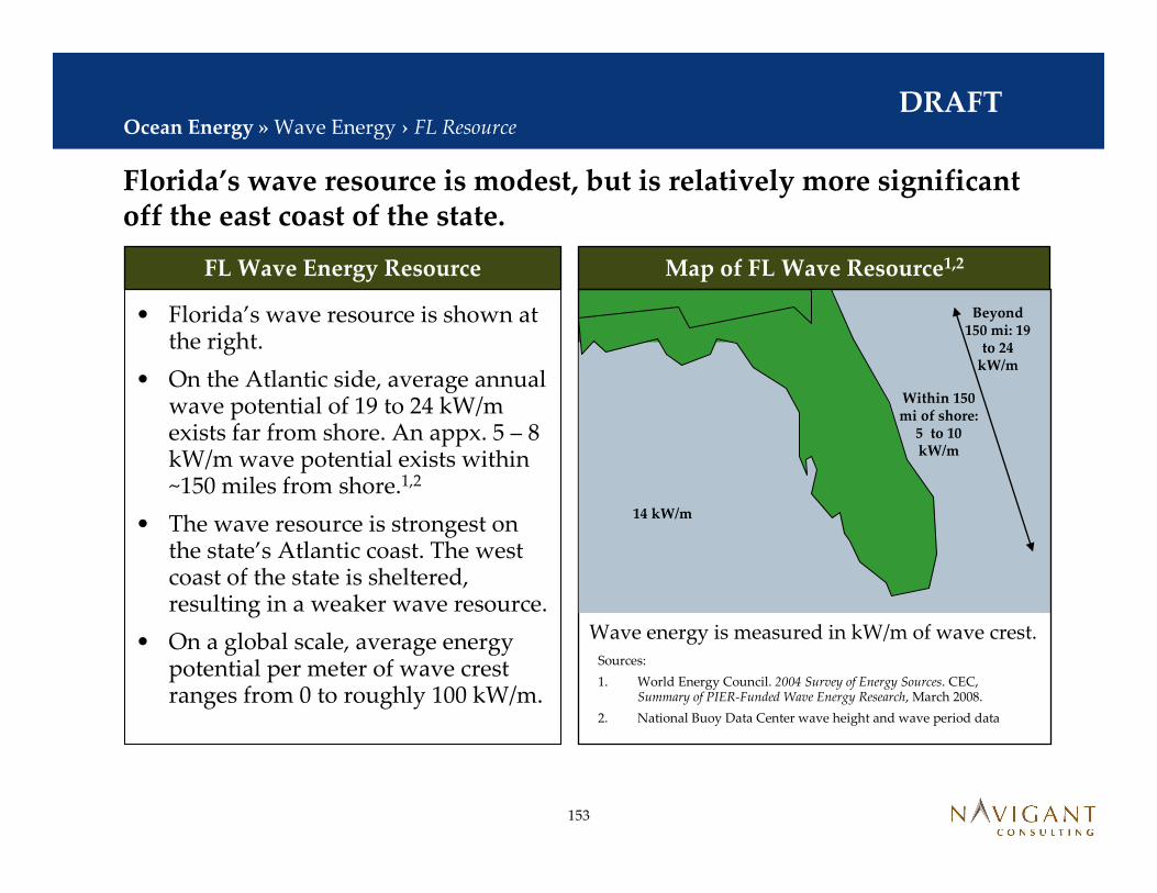


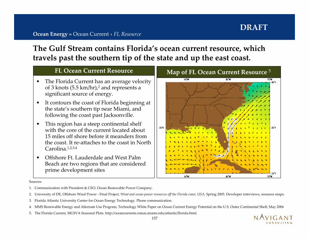

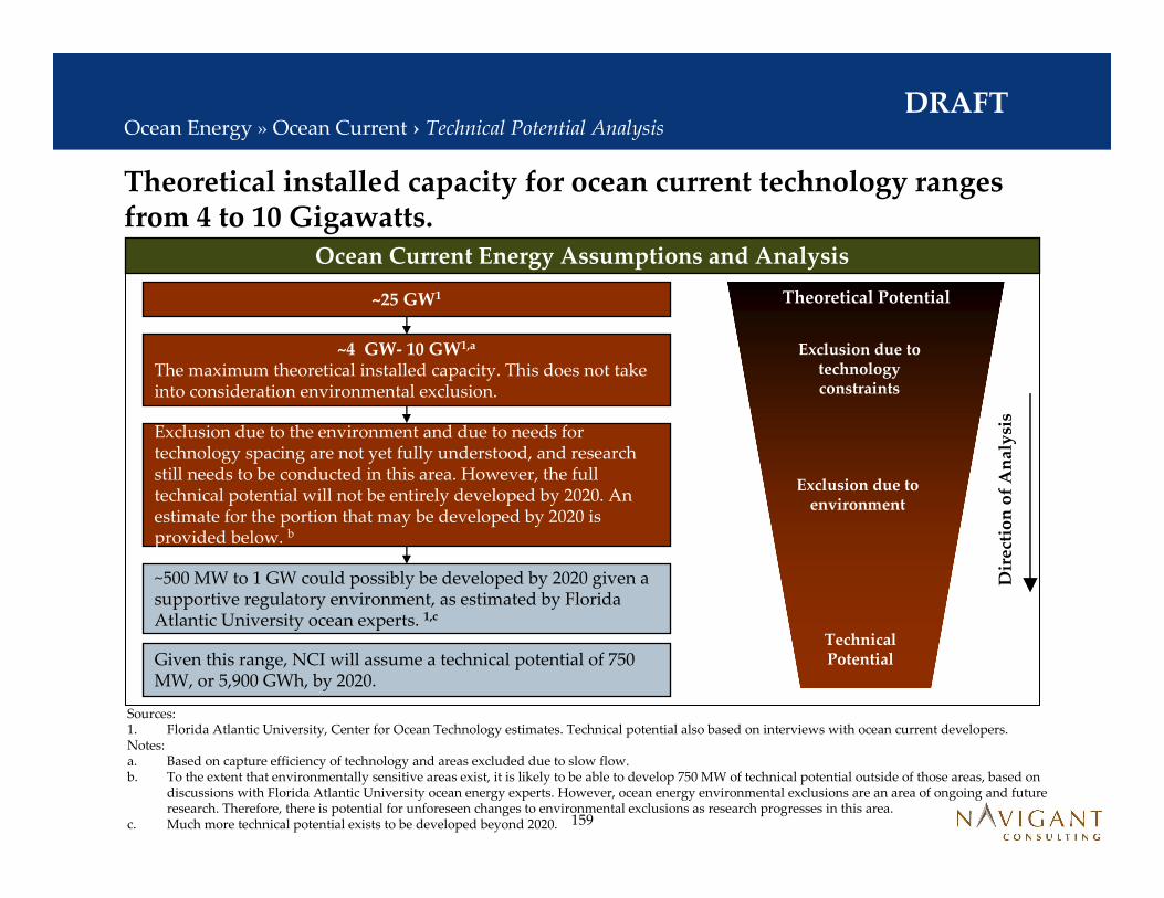

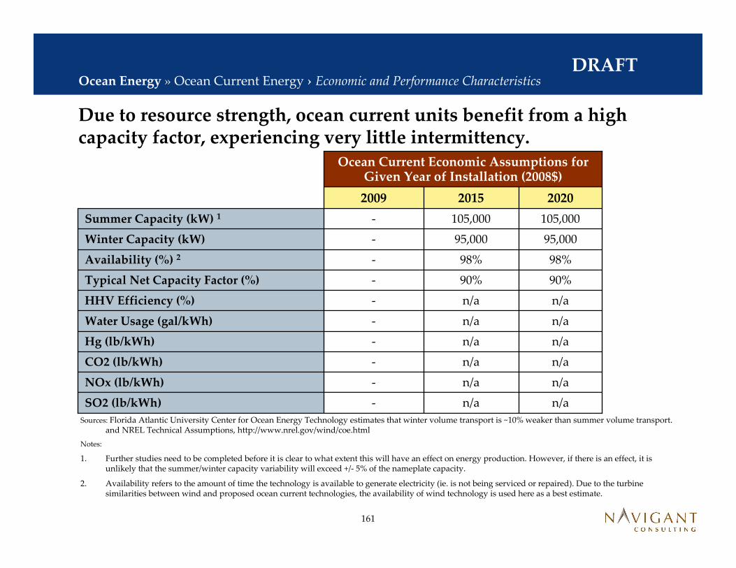

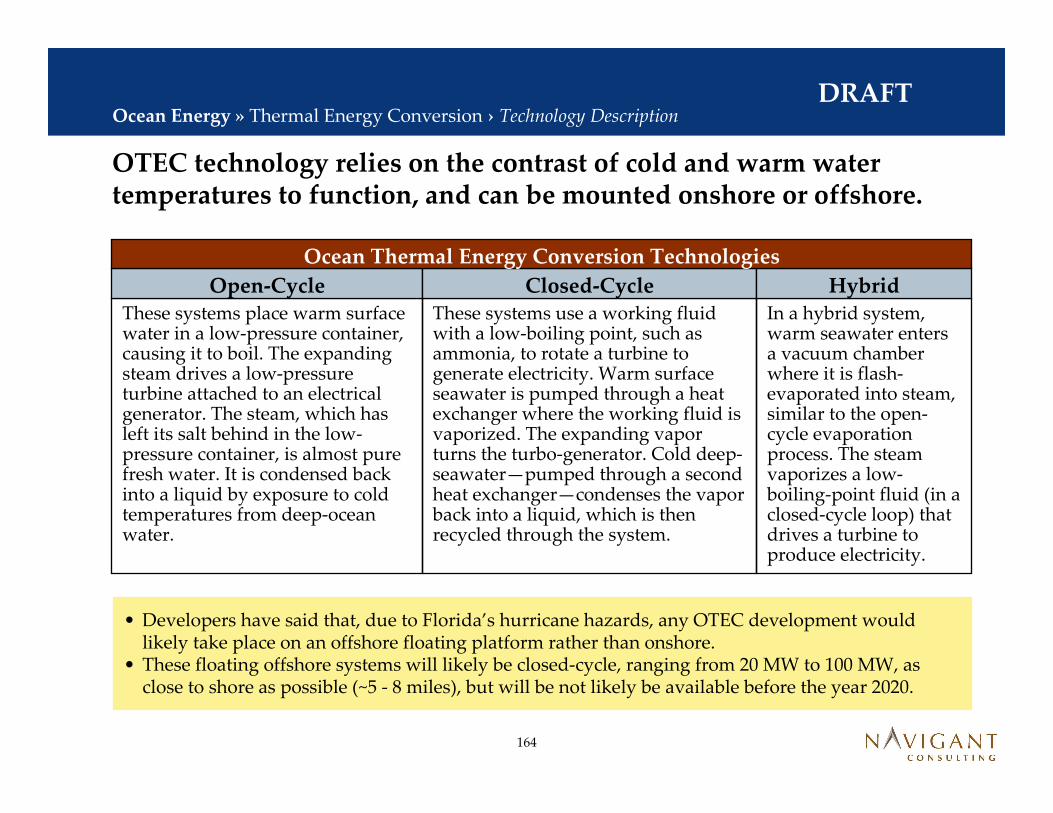
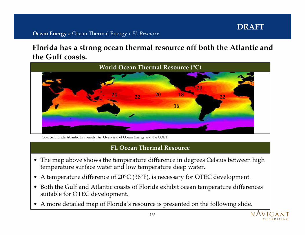
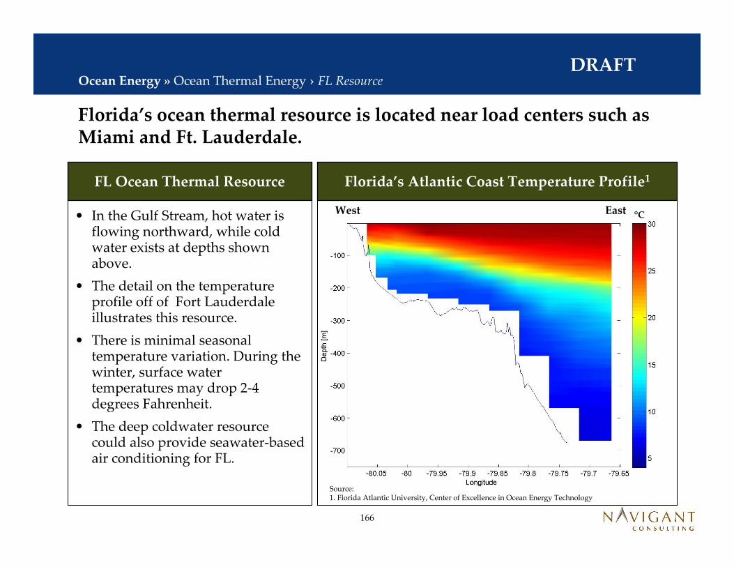

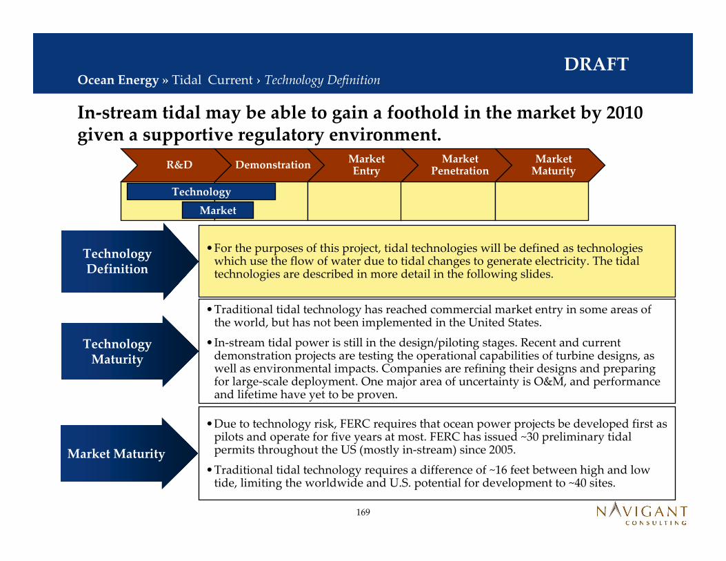
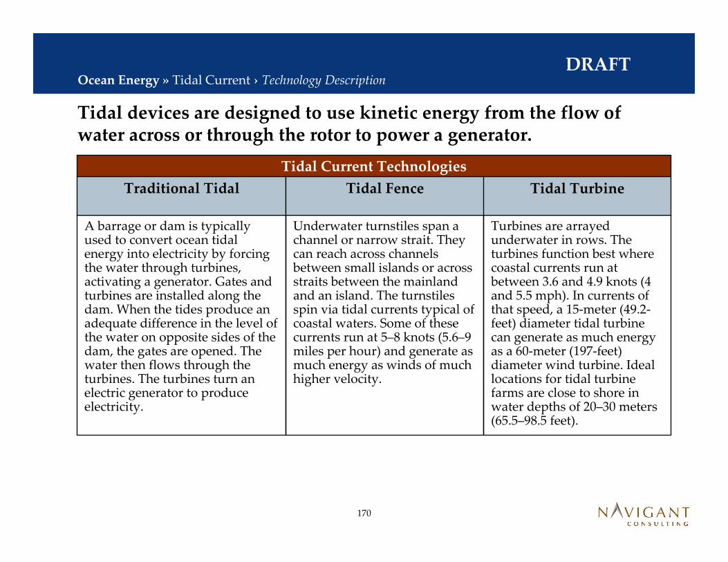
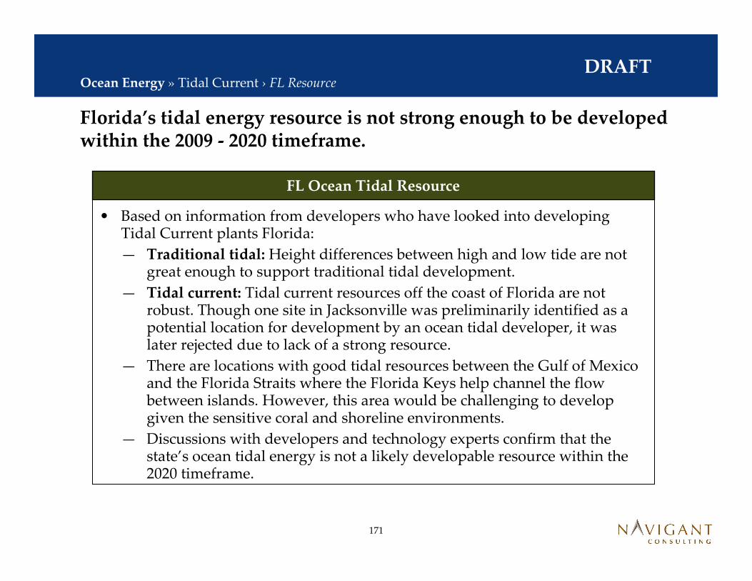

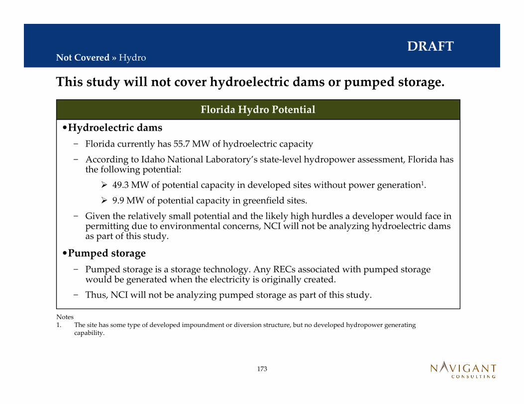

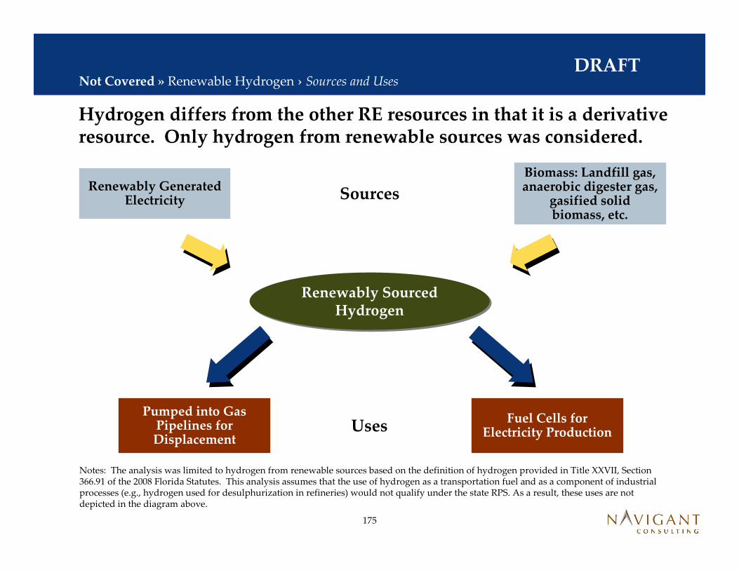
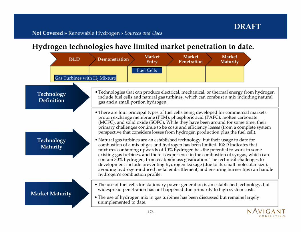
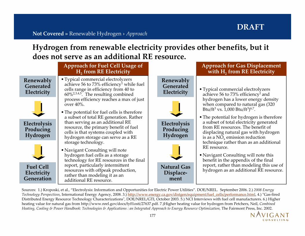
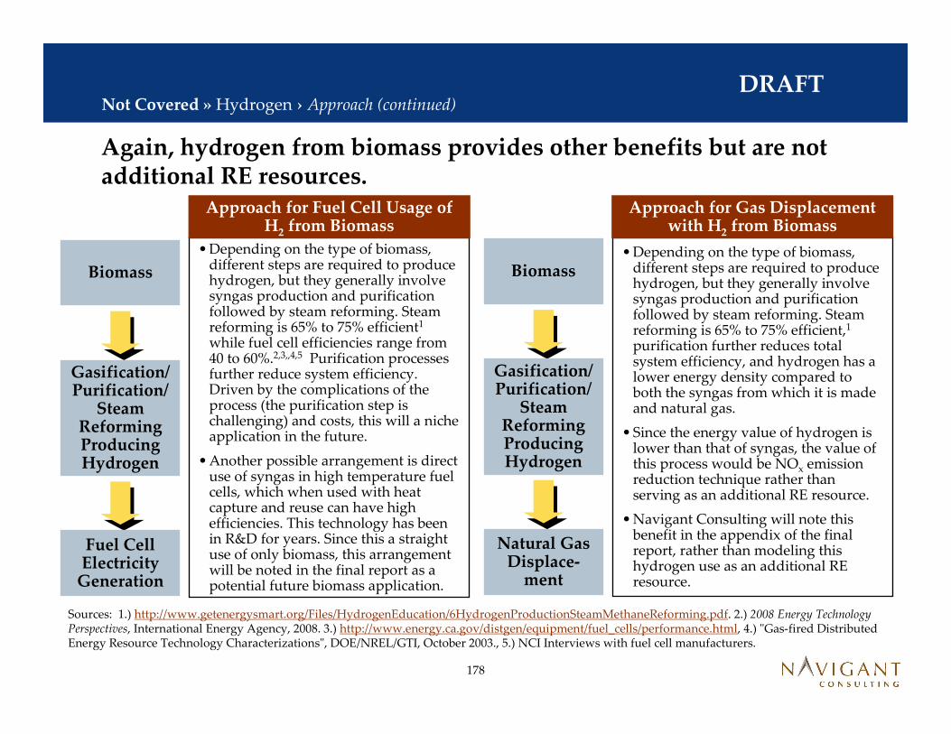
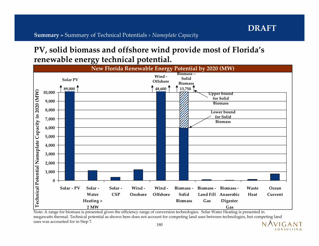
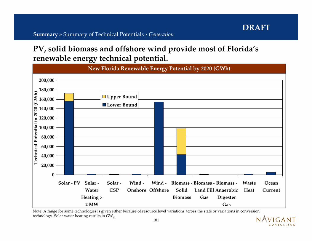
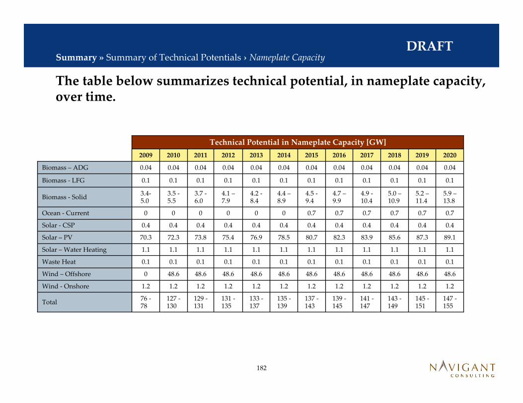


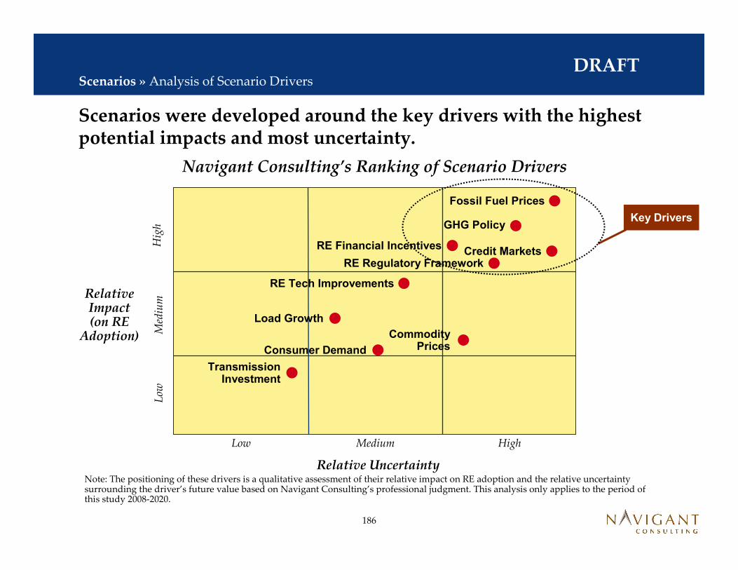
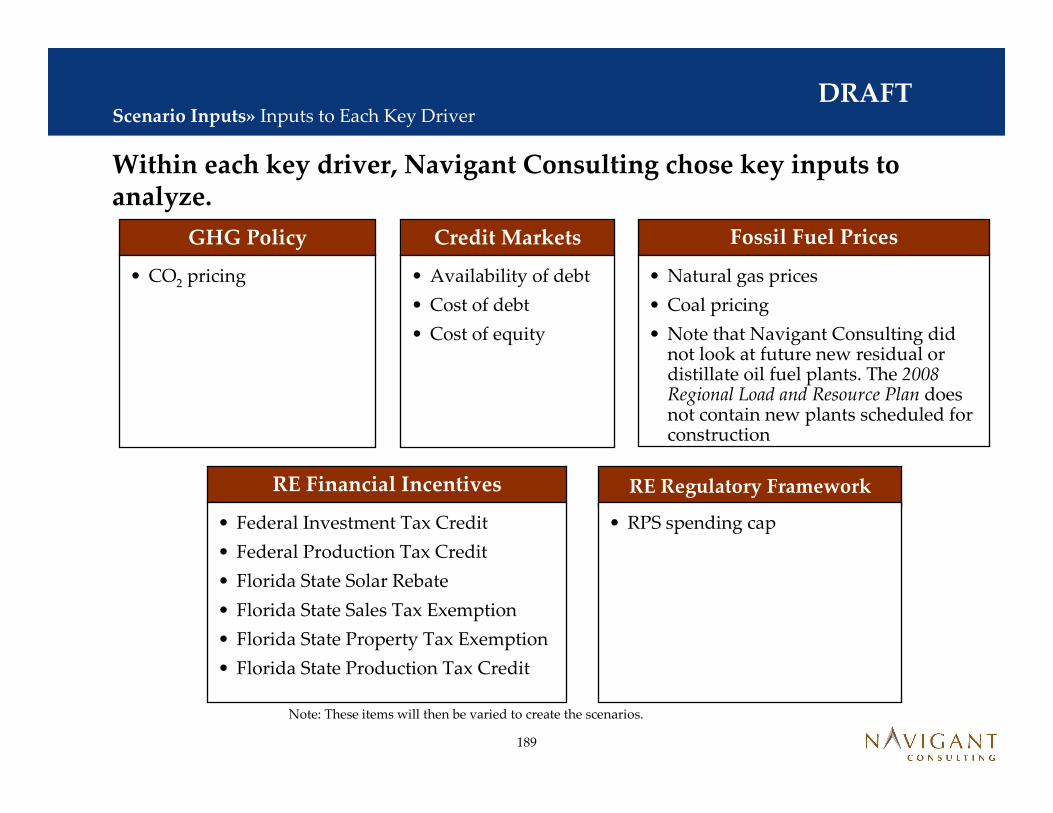
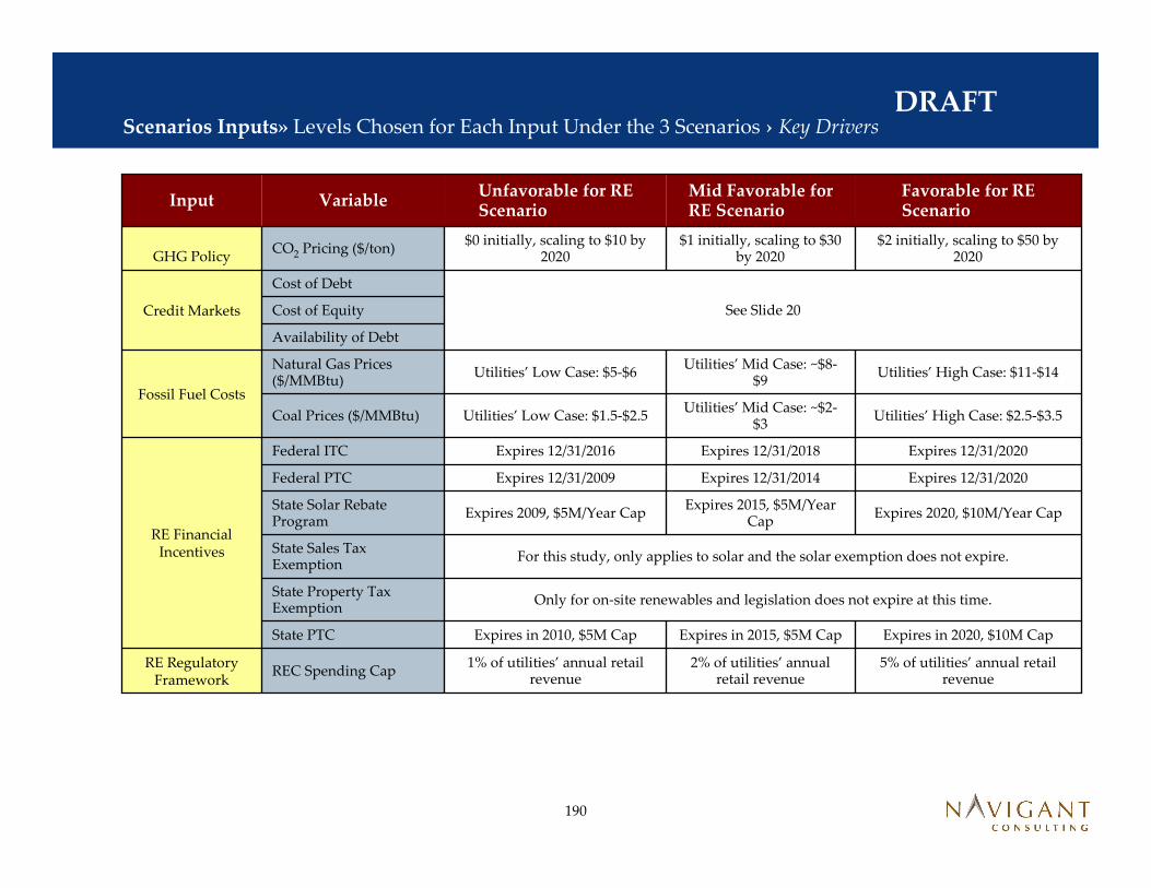

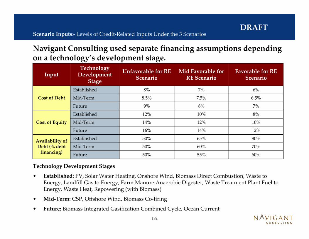


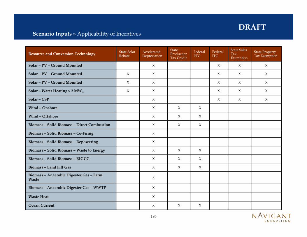
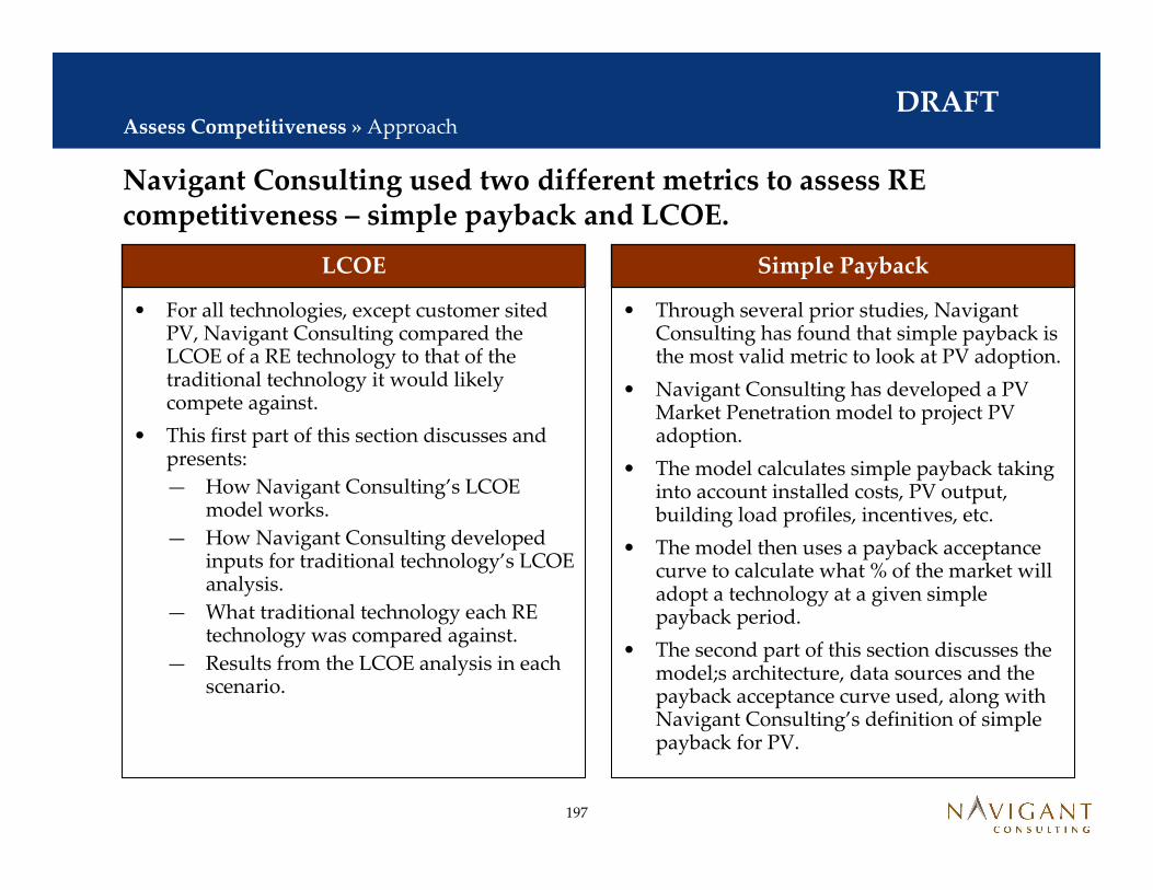


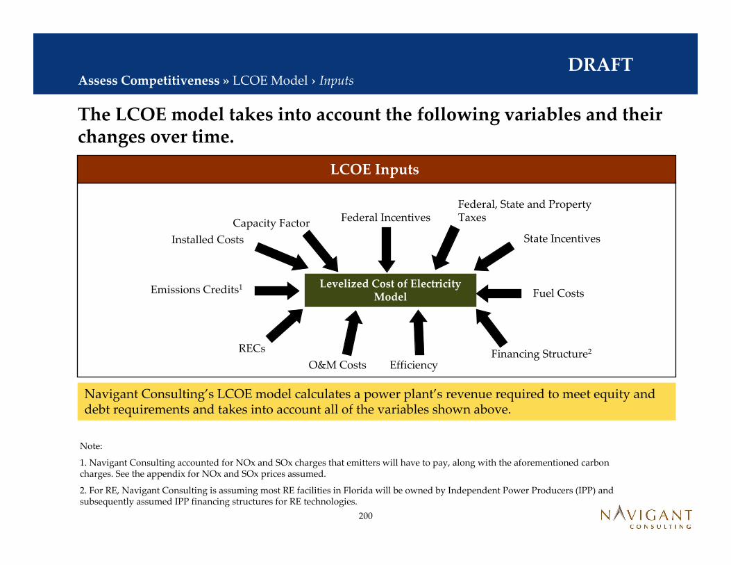
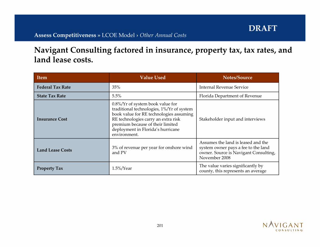
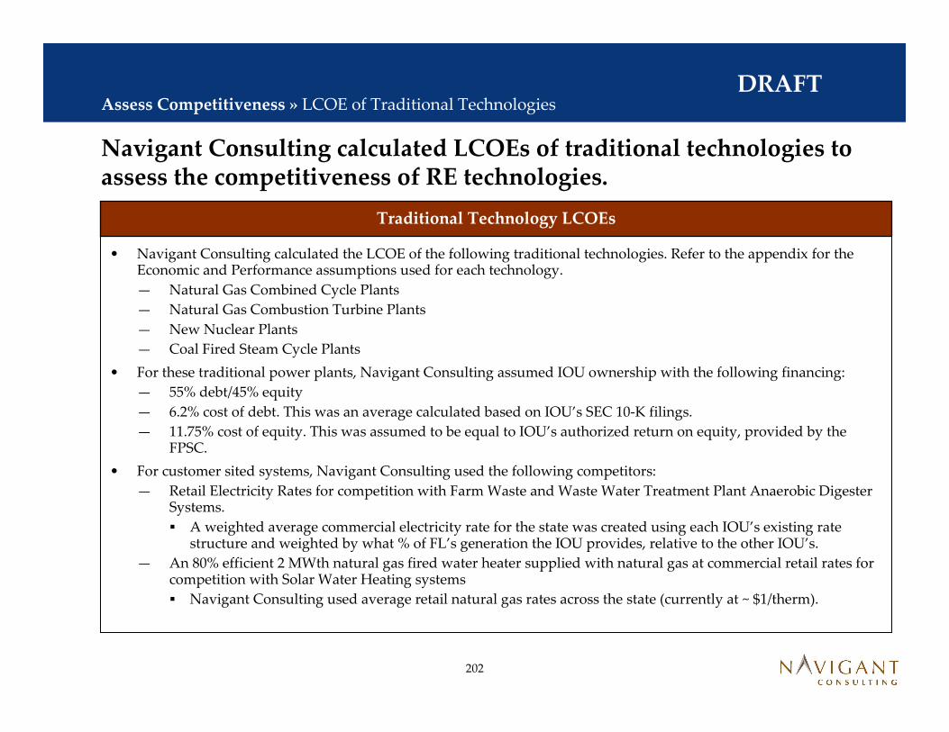

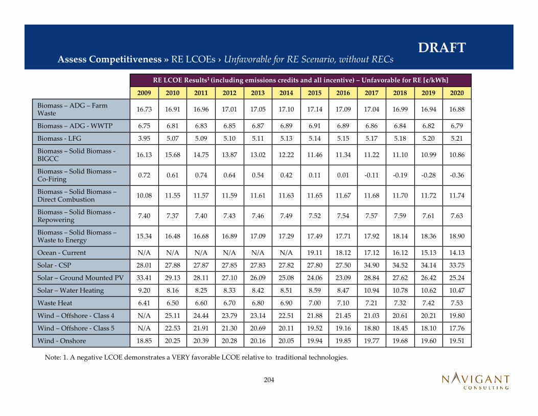

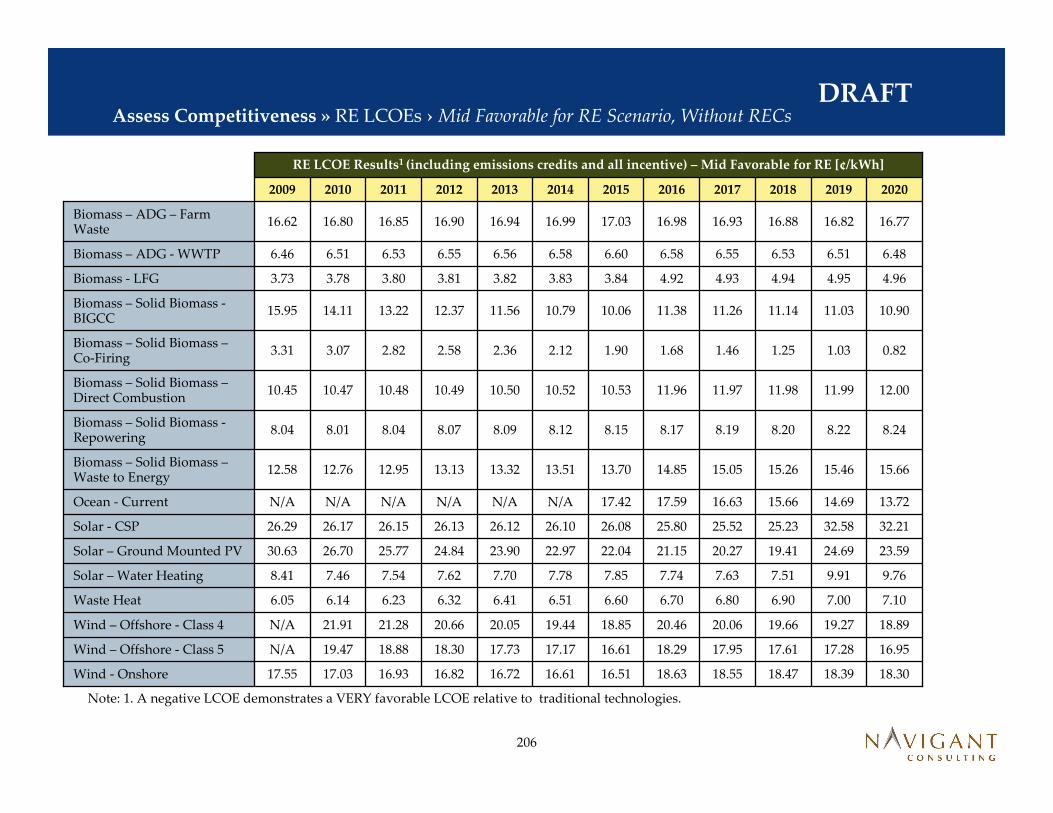
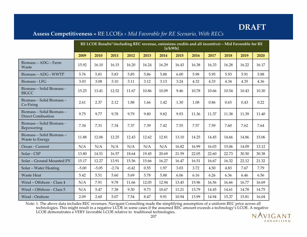


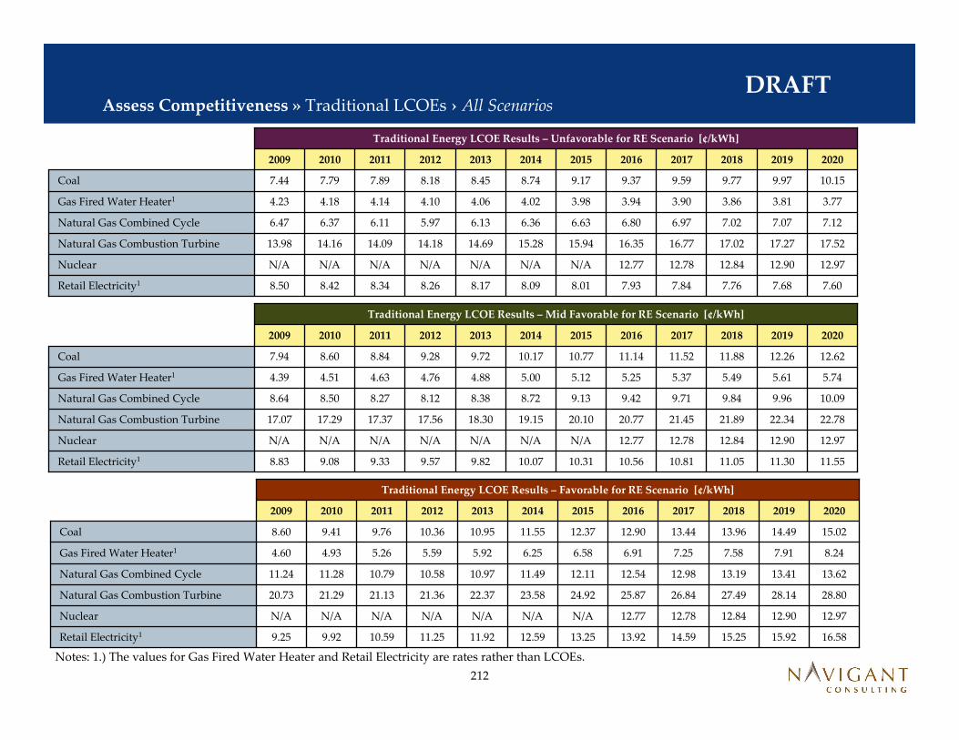

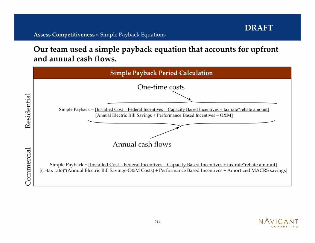


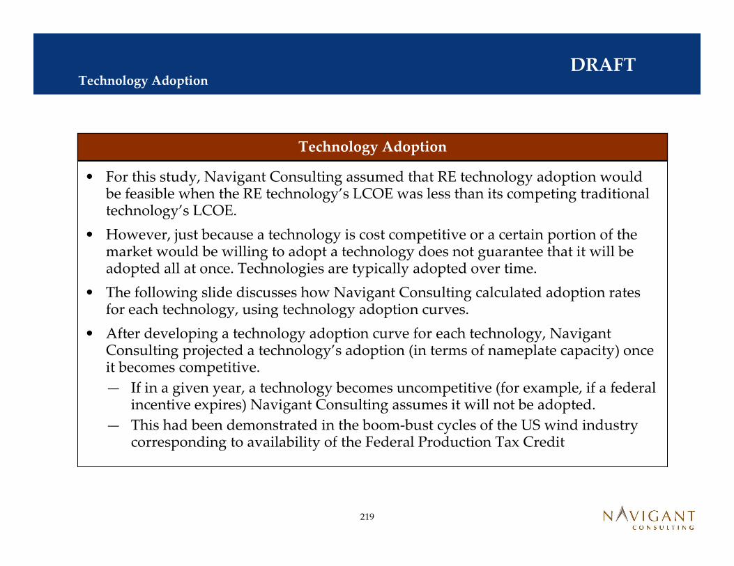

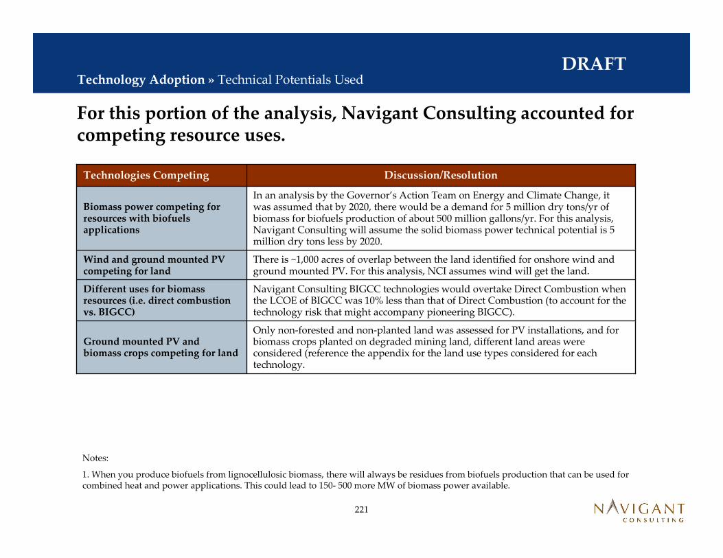

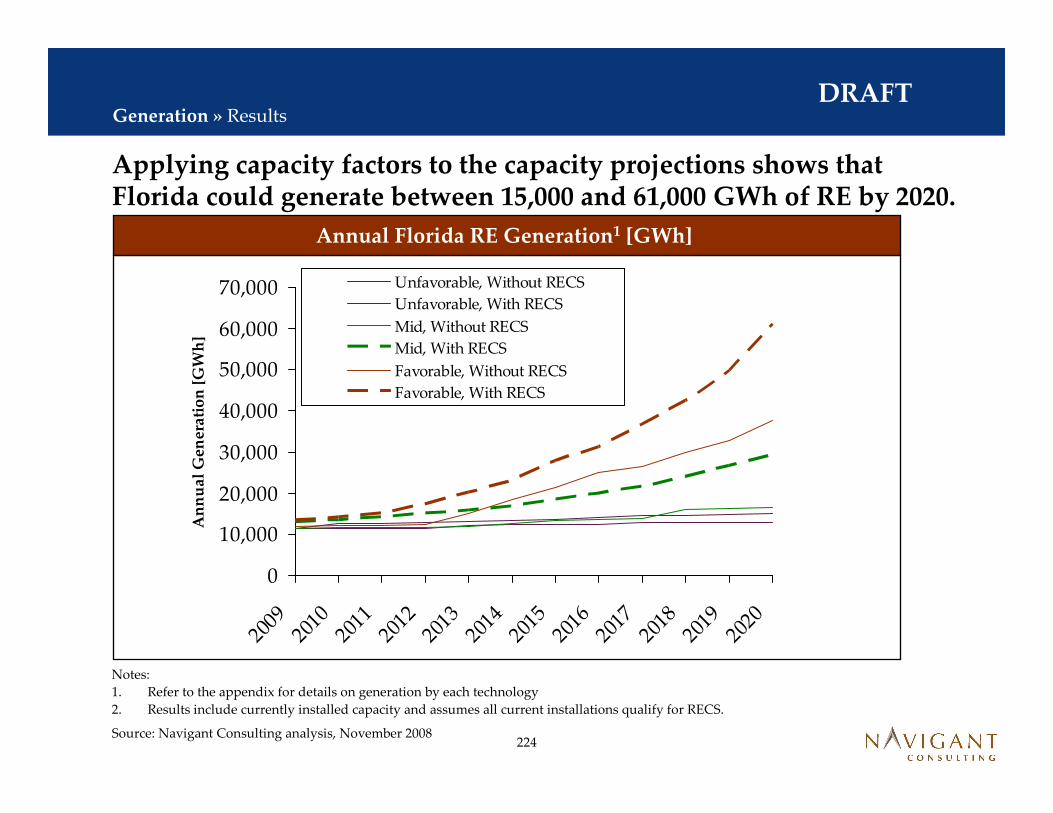
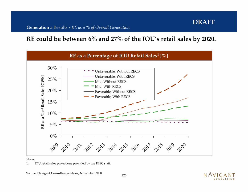

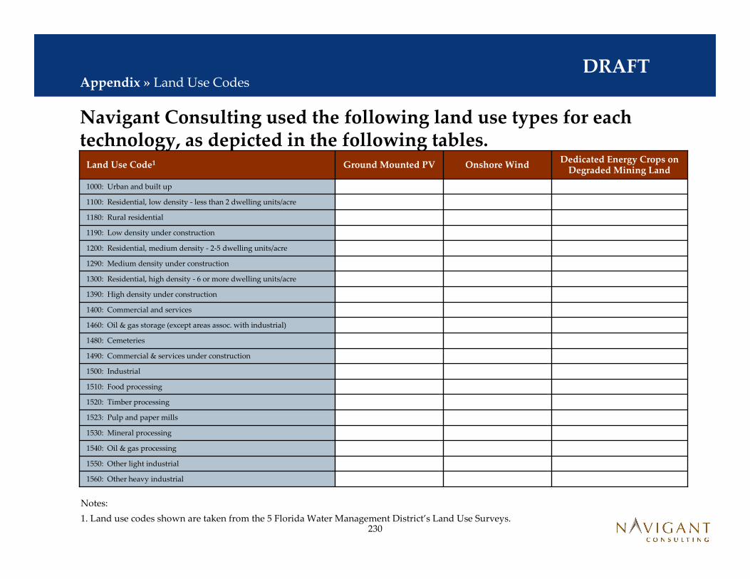
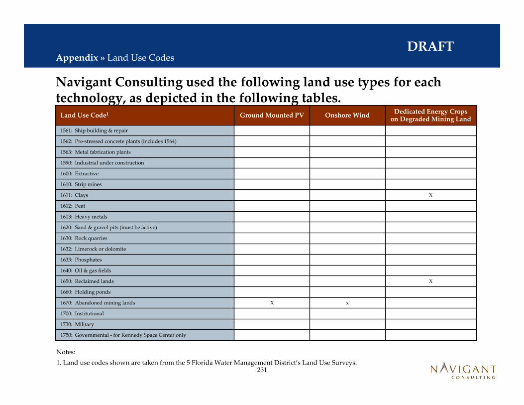
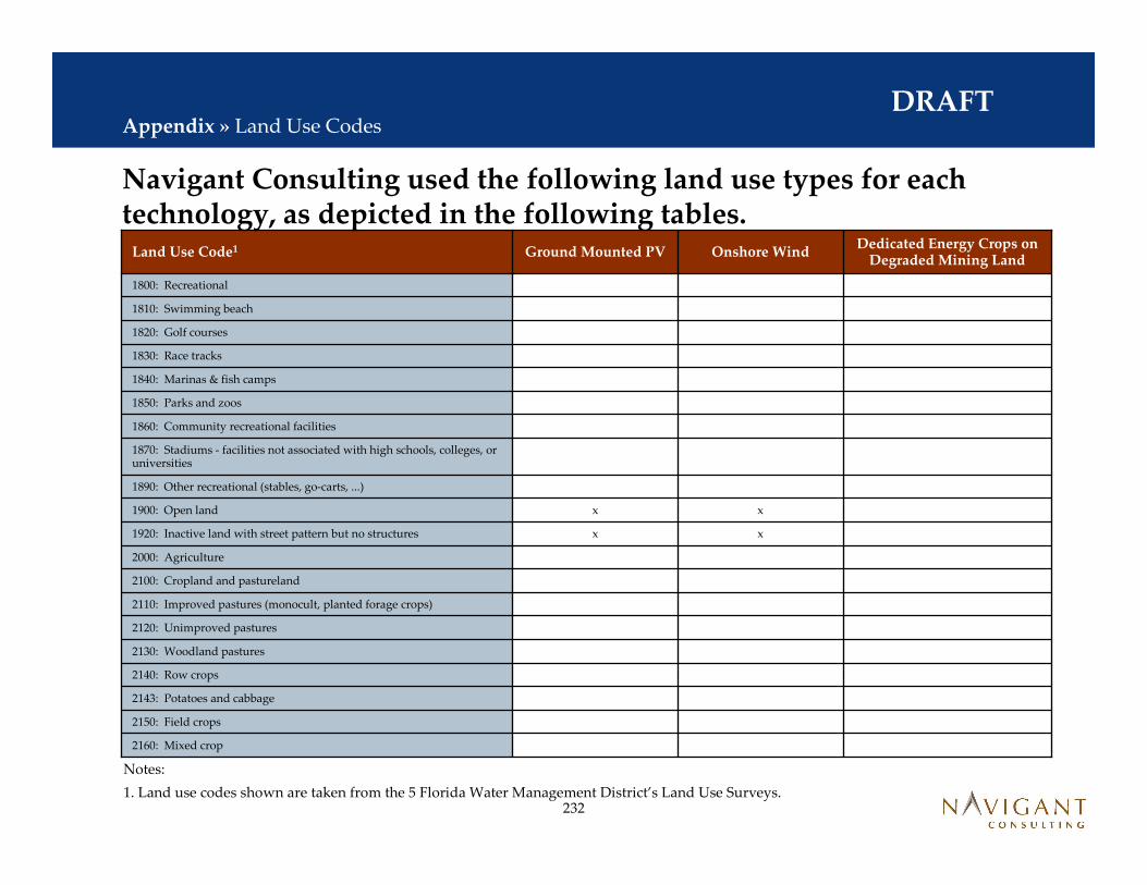
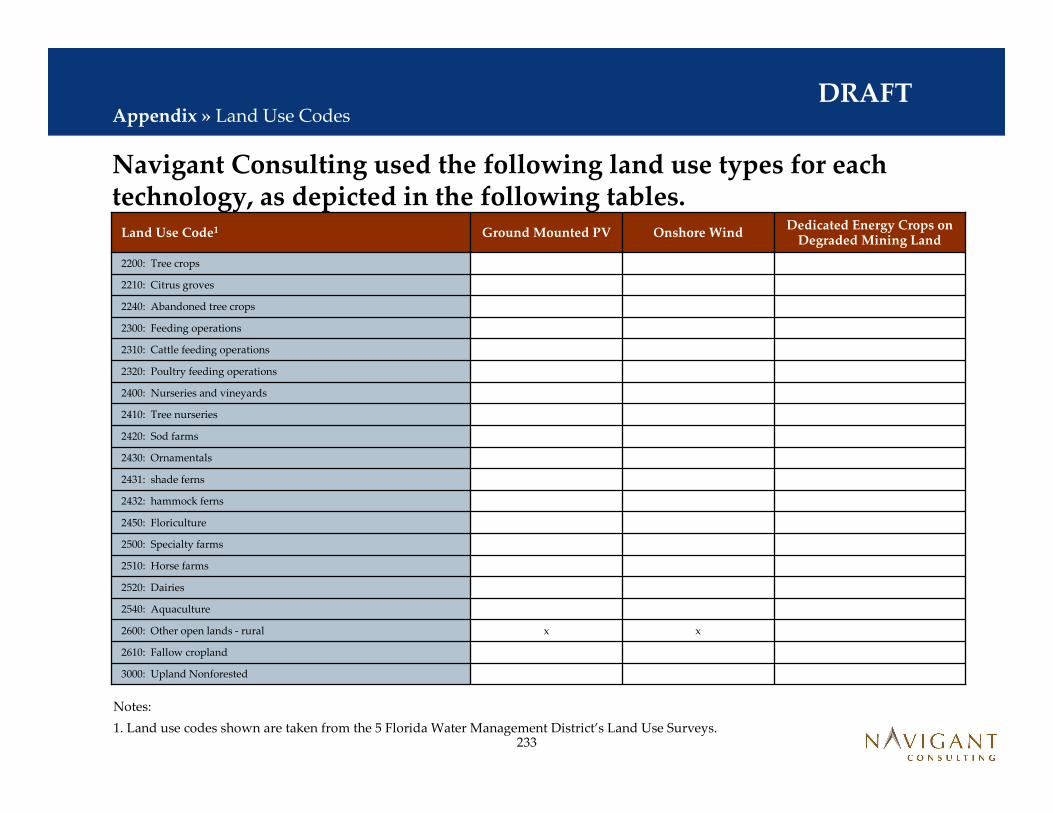
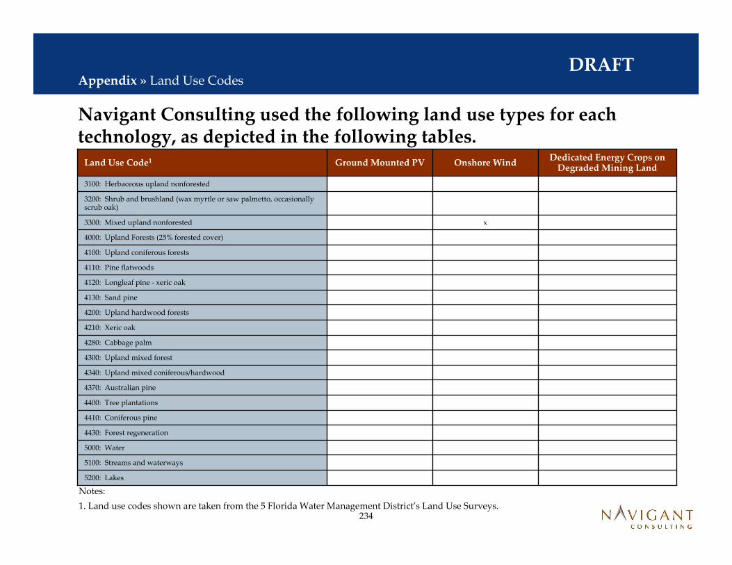


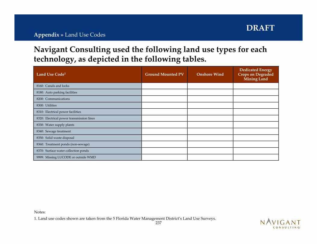


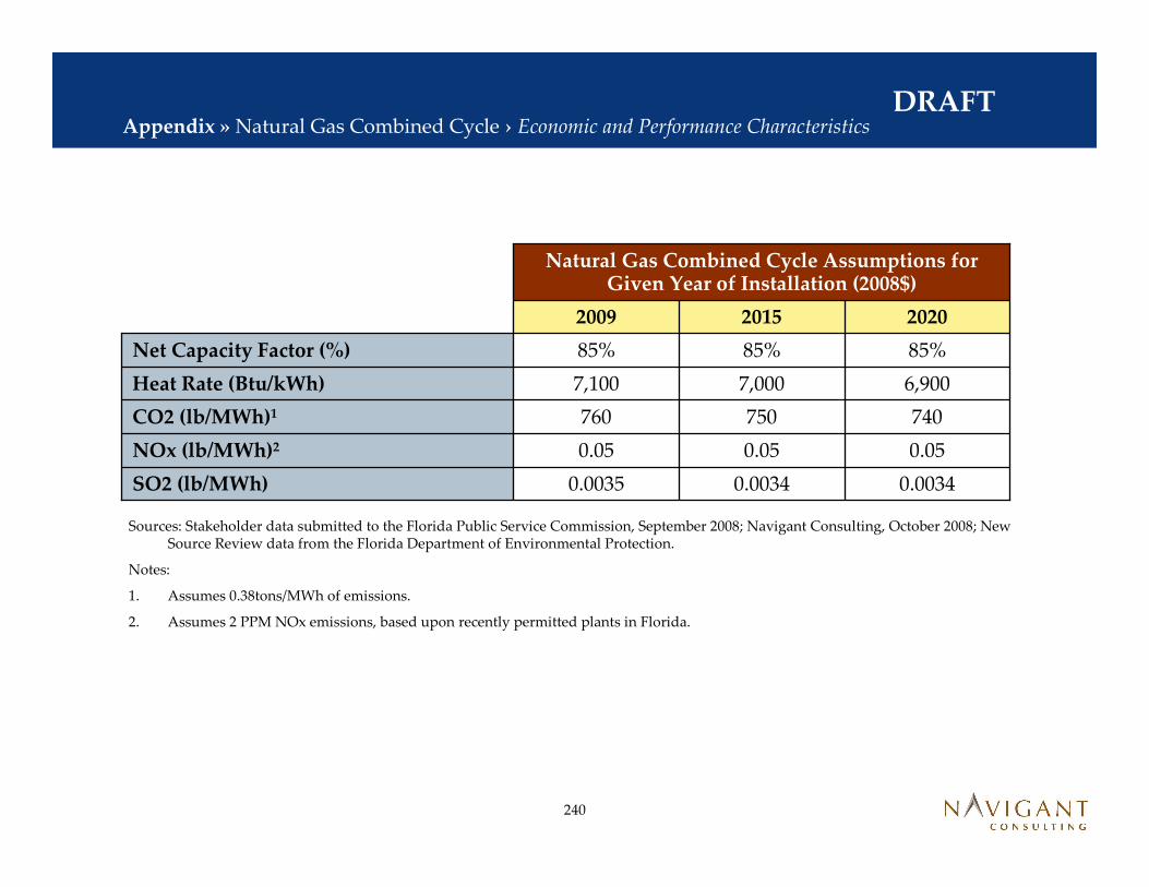
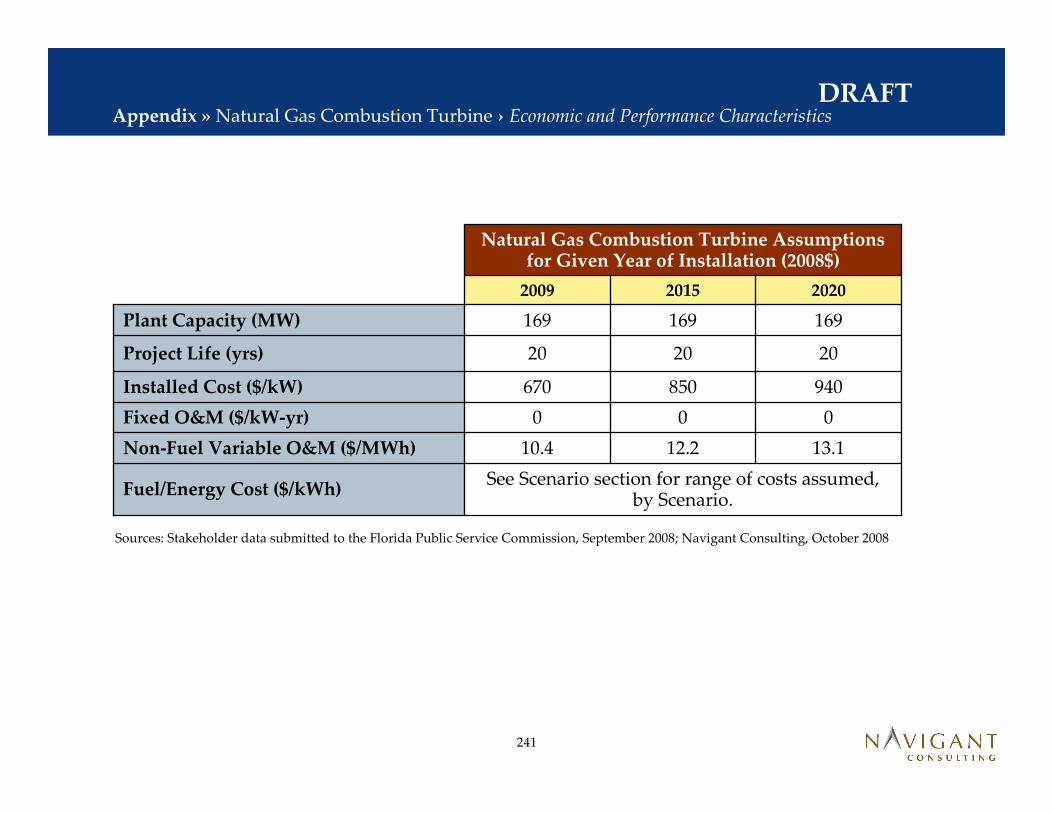


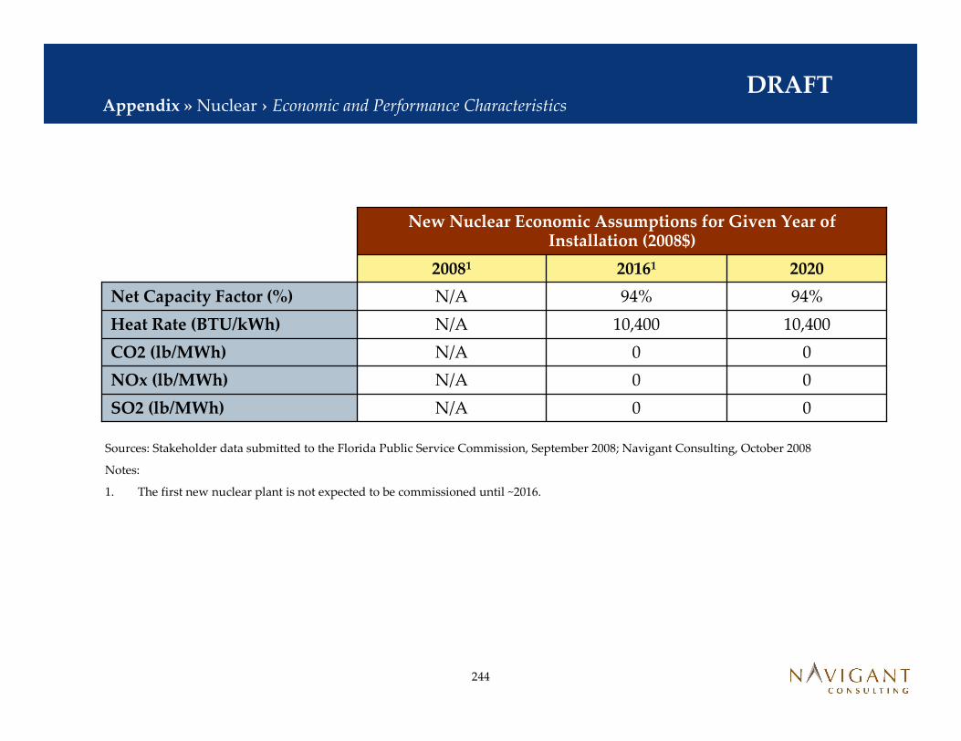

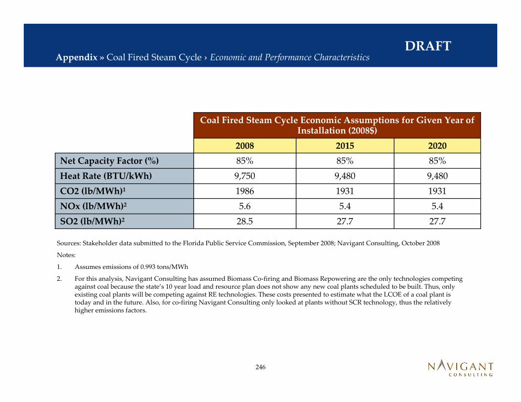
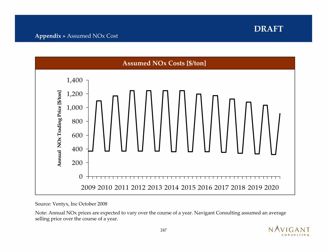
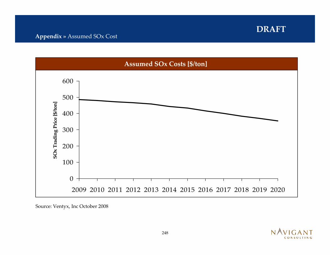
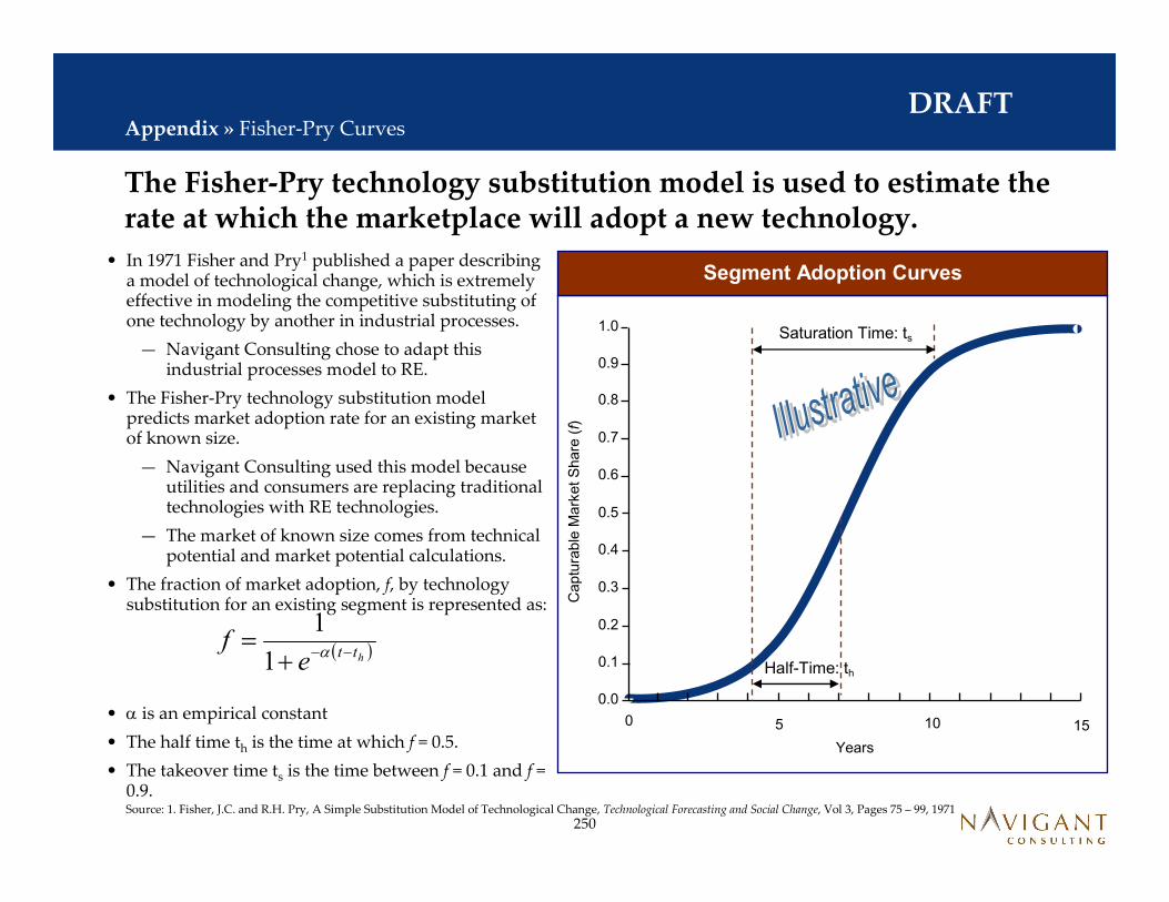
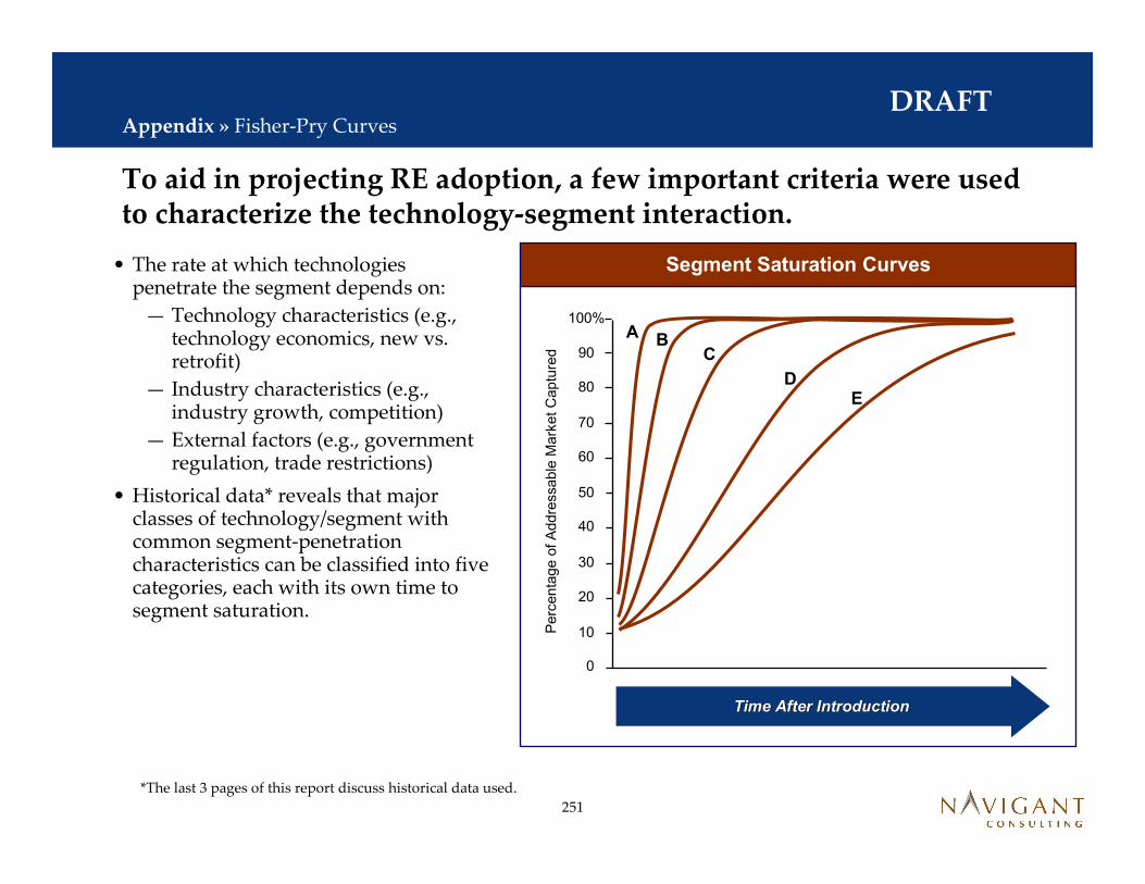
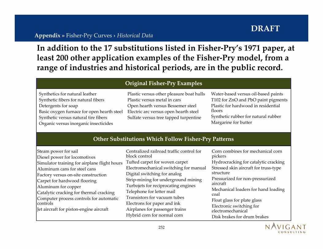
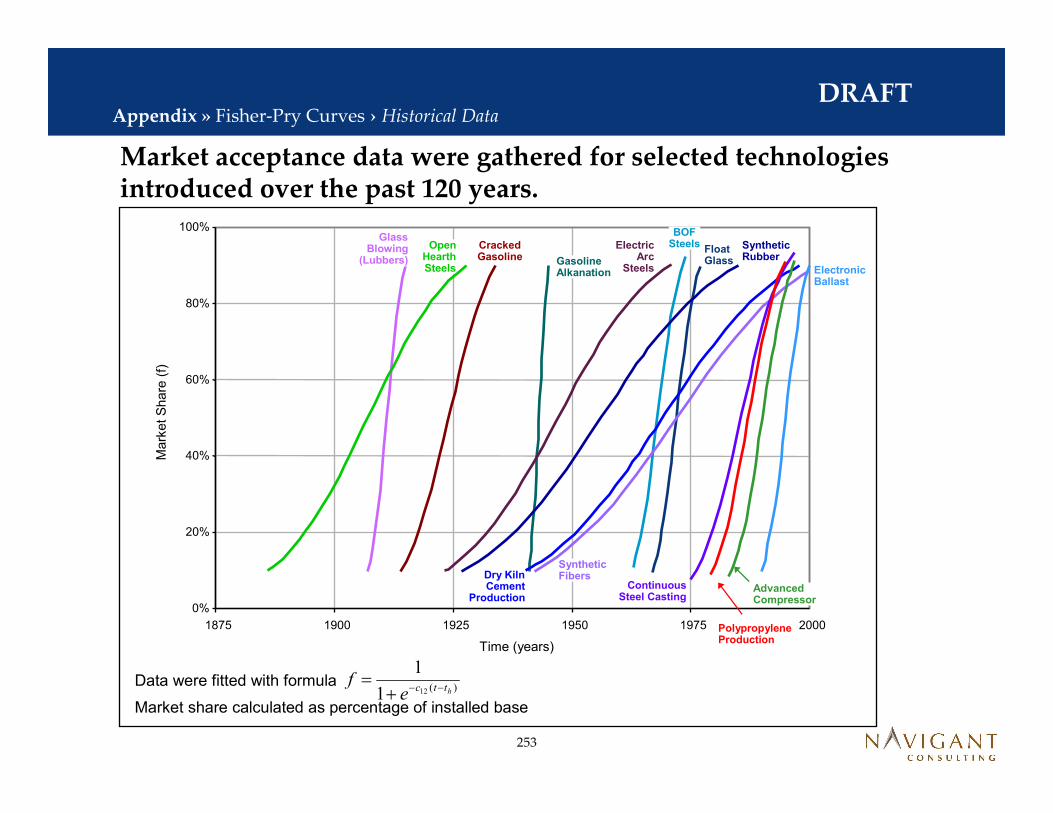
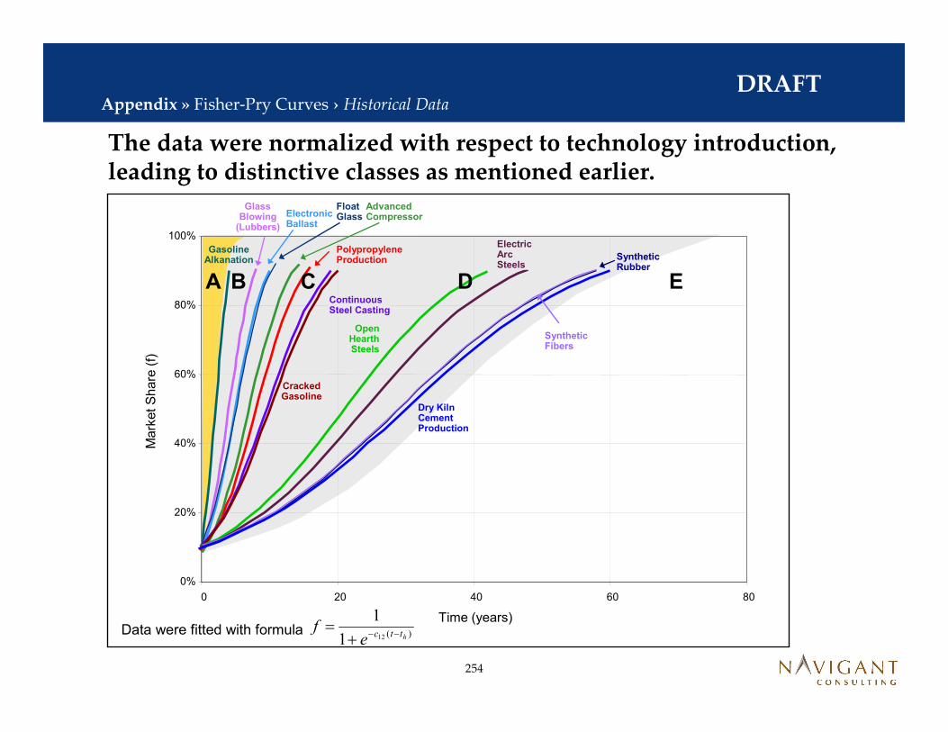


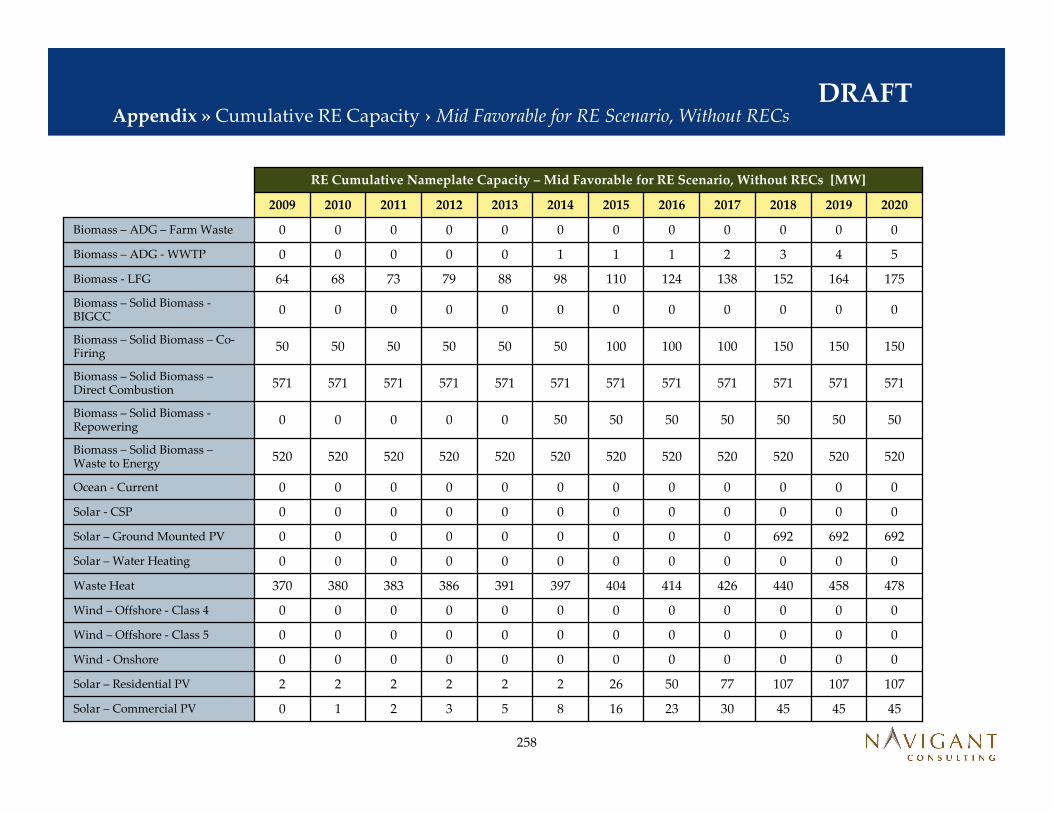
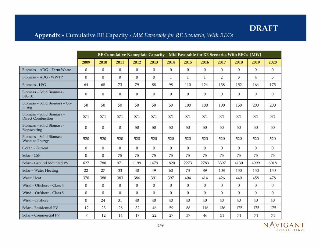

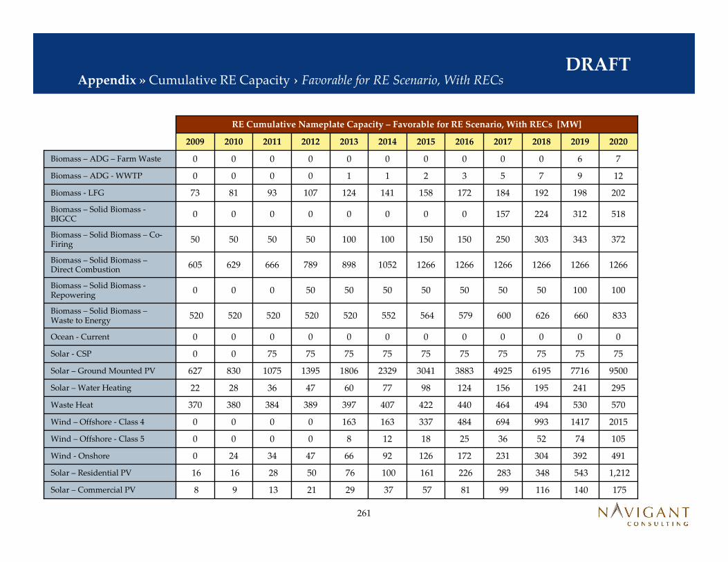


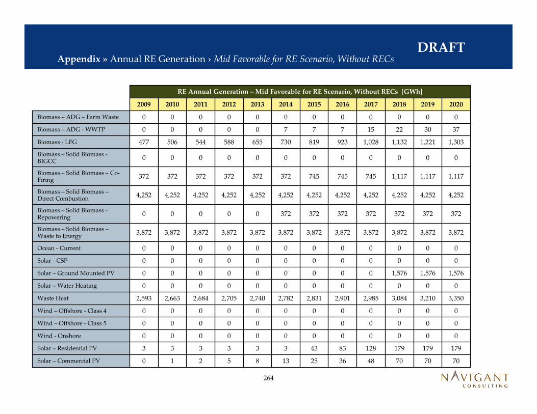


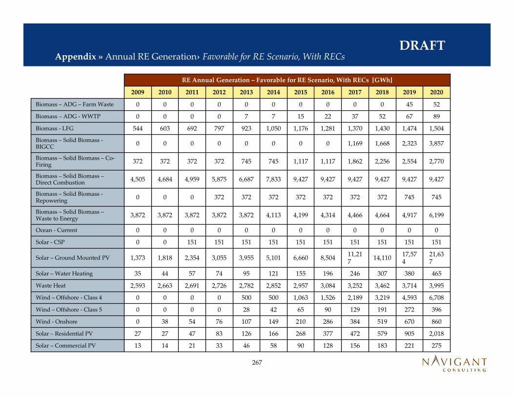

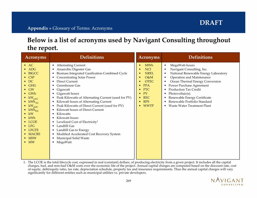


![LARGE SCALE SOLAR PV & CSP · Concentrated Solar Power (CSP). Figure 2: Ground based Solar PV System [4] Concentrated Solar Power (CSP) in contrast is a complicated technology and](https://static.documents.pub/doc/80x56/5f083bf37e708231d420ffde/large-scale-solar-pv-csp-concentrated-solar-power-csp-figure-2-ground.jpg)


